


Abstract
Automated cotton-percentage identification underpins sustainable textile recycling, but established near-infrared and ATR-FTIR spectroscopy systems cost USD 10,000–25,000 per unit and remain inaccessible to small recyclers. We address this on the CottonFabricImageBD dataset (1300 RGB originals, 13 ordinal cotton classes from 30% to 99%) and report three contributions. First, the Learnable Residual LBP stem, which retains the pretrained ResNet50 first convolution intact and adds a fully differentiable Local Binary Pattern branch as an additive contribution gated by a single learnable scalar initialized to zero, ensuring the model is numerically equivalent to the baseline at initialization (verified to a maximum absolute logit difference below ). Second, a controlled six-variant comparison (vanilla baseline, CLBP, LBP-Conv, LBP-Residual, LBP+SVM, LBP+ANN) under identical stratified five-fold cross-validation on the 1300 dataset originals. Third, the isolation of pretraining preservation as the dominant architectural variable: the 7.08 pp top-1 gap between LBP-Conv (43.77%) and LBP-Residual (50.85%), both embedding the identical learnable LBP module, is statistically significant (, uncorrected paired t-test, ) and consistent across all five folds. This gap mainly reconfirms, in the LBP setting, the established cost of discarding pretrained early-layer filters; by contrast, the improvement of LBP-Residual over the vanilla baseline (1.31 pp top-1) is consistent in direction but not statistically significant at the five-fold level (), so LBP-Residual, CLBP (50.23% top-1), and the baseline (49.54% top-1) are statistically tied on aggregate accuracy and the ranking among them is exploratory. Classical LBP+SVM and LBP+ANN baselines reach 31.85% and 34.46% top-1, confirming a genuine but limited cotton-density signal in hand-crafted descriptors. Compared to the concurrent triplet-architecture approach of Wiedemann et al. (2025), which achieves 48.15% top-1 accuracy on the same dataset under identical five-fold cross-validation, LBP-Residual attains 50.85% top-1 using a single lightweight backbone rather than an ensemble of three. These results support the design principle: augment, do not replace.
1. Introduction
The textile and fashion industry generates an enormous quantity of waste each year. According to the Ellen MacArthur Foundation, the equivalent of one garbage truck full of textiles is landfilled or incinerated every second worldwide, and only about 1% of clothing is recycled into new garments [1,2]. Mounting consumer awareness and regulatory pressure (most prominently the European Union’s recent extended-producer-responsibility frameworks and several national-level textile recycling mandates) are pushing the industry toward circularity, but a fundamental technical obstacle limits how quickly the transition can proceed: before a garment can be recycled, the fiber composition of its fabric must be known. Recycling processes (whether mechanical shredding for insulation, chemical depolymerization for new fibers, or thermal recovery for energy) are economically viable only when the input material’s composition is well characterized. The current state of practice for fiber composition identification is unsatisfactory on two fronts. Manual identification by trained textile experts using thread-counting machines and reference samples is accurate but slow, and it requires specialist labor that does not scale to the millions of garments processed daily by the industry. Spectroscopic methods, such as near-infrared (NIR) spectroscopy, attenuated total reflectance Fourier-transform infrared (ATR-FTIR), and hyperspectral imaging, are accurate at industrial throughput but require laboratory-grade equipment costing between USD 10,000 and USD 25,000 per unit [3,4,5], placing them well beyond the reach of small recyclers and developing-economy textile sectors, where much of the world’s fiber processing actually occurs. The gap between expensive accuracy and unscalable manual labor defines a clear opportunity for computer vision: a smartphone camera and a trained model could provide useful first-pass material identification at near-zero marginal cost per measurement, particularly for sorting applications that do not require the full precision of a laboratory spectrometer. This paper addresses one specific instance of that broader opportunity: estimating the percentage of cotton in a fabric from a single RGB photograph. We work with the recently released CottonFabricImageBD dataset [6], comprising 1300 fabric images spanning 13 cotton percentage classes from 30% to 99%, captured with a consumer smartphone and labeled under expert supervision using thread-counting verification. The dataset is the first public benchmark targeting cotton percentage as an ordinal classification problem, and its construction provides ground-truth labels at the same level of precision that laboratory-grade methods achieve, making it a clean benchmark for evaluating low-cost alternatives.
Cotton percentage is fundamentally a thread-density measurement. The dataset authors compute it by counting horizontal and vertical threads under a magnifying glass and dividing by the count of an idealized 100% cotton reference [6]. In computer vision terms, this is a texture problem: the discriminative signal lives in the high-frequency periodic structure of the weave, not in shape, color, or global composition. Different cotton percentages produce visually similar fabric photographs that differ primarily in the fine-scale spatial pattern of fiber arrangement.
It is worth stating explicitly why this problem needs more than an off-the-shelf CNN, given that CNN image recognition is otherwise mature. Three features are specific to the textile setting. First, the discriminative signal is high-frequency weave micro-texture, not object shape or color; standard ImageNet-trained CNNs are known to be shape-biased [7], so they are, if anything, mismatched to fabric-density estimation and benefit from an explicit texture prior. Second, labeled data are scarce and expensive: ground-truth cotton percentage requires expert thread-counting under magnification, so textile datasets are small (1300 originals here), which makes preserving pretrained early-layer features far more consequential than in large-scale vision. Third, the deployment target is a low-cost, smartphone-grade sorting aid without laboratory equipment, which rewards a single lightweight backbone carrying a small, interpretable, baseline-bounded texture module over heavy multi-backbone ensembles. The residual LBP stem is designed around exactly these three constraints, which distinguishes it from simply applying a generic high-capacity recognition network to fabric images.
Modern CNNs are well known to be biased toward shape over texture [7]. Classical computer vision developed dedicated texture descriptors for this setting. Among them, Local Binary Patterns (LBP) [8,9] and its Completed LBP variant [10] are particularly suited to encoding local microstructure as illumination-invariant binary codes. LBP was selected specifically over alternative texture descriptors for three reasons. First, LBP admits a fully differentiable formulation: the learnable LBP module we introduce in Section 3.5 (with learnable neighbor offsets via bilinear interpolation, sigmoid thresholding, and a learnable encoding matrix) makes the descriptor end-to-end trainable; this module is our own construction and extends the parameter-efficient binary-convolution idea of Ref. [11], whose binary patterns are randomly initialized and fixed rather than tied to classical LBP, enabling end-to-end gradient training. Second, it is illumination-invariant under monotonic gray-scale transformations, which is particularly relevant for smartphone-captured fabric images with variable lighting. Third, its binary-code representation directly encodes the spatial periodicity of weave structure that corresponds to thread density. By contrast, Gray-Level Co-occurrence Matrices (GLCM) lack a straightforward differentiable formulation for end-to-end learning; Gabor filters are less compact for encoding binary weave structure; and learnable texture networks typically require larger datasets than the 1300 originals available here.
The most directly related prior work is Wiedemann et al. [12], who recently proposed a triplet-loss metric-learning architecture combining DenseNet121, EfficientNetB4, and ResNet50 backbones with adaptive feature pyramid networks and deformable convolutions for cotton-content classification. Our work differs from theirs in two complementary ways: methodologically, we treat cotton content as an ordinal classification problem with a Gaussian soft-label objective rather than as a metric-learning problem; architecturally, we contribute a single principled augmentation (the residual LBP stem with a learnable scalar gate initialized to zero) to a standard pretrained ResNet50, rather than ensembling multiple backbones with specialized attention mechanisms. The simplicity of our design supports the interpretability advantage we describe in Section 3.6, and the residual-gate template should compose with the metric-learning and multi-backbone approaches of Wiedemann et al. in principle.
A subtle but consequential issue arises when integrating LBP at the input layer of a pretrained network: the pretrained ImageNet weights at that layer are discarded, and the network must relearn first-layer filters from scratch on the (typically small) target dataset. On large datasets this is recoverable; on small datasets it is catastrophic, because first-layer filters in CNNs encode universal visual primitives (oriented edges, color-opponent gradients, Gabor-like patterns) that take a substantial amount of training data to learn well from random initialization [13]. With only 1300 originals in the CottonFabricImageBD dataset, this is squarely in the small-data-and-pretraining-matters regime. This creates a tension at the heart of LBP-CNN integration on small datasets. We want the LBP signal early in the network, where it can shape downstream representations and provide the strongest possible inductive bias for texture features. But injecting LBP early typically requires modifying the pretraining-rich first convolution, exactly the layer where preserving pretrained representations matters most.
We propose a simple but principled design we call the residual LBP stem. The pretrained first convolution of a ResNet50 is retained exactly as-is. Alongside it, we add a learnable LBP branch (a fully differentiable LBP encoder operating on the luminance channel) whose output is added to the pretrained convolution’s feature map, gated by a single learnable scalar initialized to zero:
Three properties make this design useful. First, at initialization, the model is mathematically identical to the baseline since collapses the equation to the pretrained convolution alone (verified empirically to within a maximum absolute logit difference of ). Second, the worst-case behavior is bounded by the baseline: if LBP features turn out to be uninformative, remains near zero, and the model recovers baseline performance. Third, the gate value provides post hoc interpretability: its converged magnitude directly indicates whether the network actually exploited the auxiliary stream during training.
To establish what classical pre-deep-learning techniques achieve on this task and provide a reference point for the deep variants, we additionally evaluate two non-deep baselines: a multi-class Support Vector Machine with RBF kernel and a shallow multi-layer perceptron, both operating on 160-dimensional spatial LBP histograms (4 × 4 grid of uniform-LBP features). These methods do not use any pretrained representations and operate entirely on hand-crafted descriptors. Including them allows us to ask not just whether deep features beat classical features (they do) but by how much, and whether the cotton-density signal is recoverable at all from classical LBP descriptors. The answer to the latter question turns out to be informative: classical LBP carries genuine but limited cotton-density signal, which strengthens rather than weakens the case for the residual hybrid design.
Beyond the architectural proposal, this paper makes two additional methodological contributions. First, we adopt an explicitly ordinal evaluation protocol: we use mean absolute error (MAE) in percentage points as the primary metric, adjacent-class accuracy as a complementary metric, and a Gaussian soft-label cross-entropy loss whose target distribution decays smoothly with percentage distance. Standard top-1 accuracy treats predicting 95% as equally wrong as predicting 30% when the true label is 99%; an ordinal protocol correctly weights these errors by their ordinal magnitude. Second, we identify and document a methodological pitfall in the CottonFabricImageBD release: the 27,300 pre-augmented images cannot be cleanly split for cross-validation because the augmentation file naming does not preserve the mapping between augmented files and their source originals. Naively splitting across the augmented set places near-duplicates of training images into the validation fold and inflates apparent accuracy by tens of percentage points. We split exclusively on originals and apply augmentation on the fly during training, which we believe should become the standard protocol for this dataset.
We compare six model variants under stratified five-fold cross-validation on the CottonFabricImageBD originals: a vanilla ResNet50 baseline, three deep LBP-augmented variants (CLBP input augmentation, LBP-Conv replacement stem, and the proposed LBP-Residual additive stem), and two classical baselines (LBP+SVM and LBP+ANN). Our experiments show the following:
- The proposed Residual LBP variant achieves the best top-1 (50.85% vs. 49.54% baseline) and top-3 (84.77% vs. 83.69%) accuracy among the deep variants (the best on two of the four primary metrics) while essentially tying the baseline on adjacent-class accuracy (84.92% vs. 85.15%) and CLBP on MAE (5.70 pp vs. CLBP’s 5.68 pp). Improvements over the baseline are consistent across folds, with a 28% reduction in MAE standard deviation, but fall within cross-validation noise.
- The LBP-Conv variant, which replaces rather than augments the pretrained first convolution, performs substantially worse than the baseline (43.77% top-1 accuracy, 7.69 pp MAE). The seven-percentage-point gap between LBP-Conv and LBP-Residual, two variants embedding the identical learnable LBP module, points to pretraining preservation as the dominant architectural variable on small textile datasets (the two variants also differ in fusion mechanism, a residual confound discussed in Section 5.1); this gap largely reconfirms the known cost of discarding pretrained early-layer filters [13], whereas the separate and genuinely novel question (whether the zero-gated residual improves over a strong pretrained baseline) is answered only weakly, by a consistent but non-significant gain (Section 4.1).
- The classical baselines achieve 31.85% (LBP+SVM) and 34.46% (LBP+ANN) top-1 accuracy, 15–19 percentage points below the deep variants but 4–5× above the random-chance floor. This confirms that classical LBP histograms carry genuine but limited cotton-density signal.
- The residual gate moves away from zero on all 5 folds (end-of-training ), which shows that the optimizer did not switch the LBP branch off. Because the magnitude of is not identifiable (Section 3.6), this indicates only that the branch was used, not how much it contributes.
We interpret these findings as supporting a general design principle for hybrid hand-crafted/deep architectures on small datasets: augment, do not replace. Whenever auxiliary features can be expressed as a residual addition to a pretrained layer’s output, the residual formulation should be preferred to a replacement formulation, since the worst-case behavior of the residual variant is bounded by the baseline while the worst-case behavior of the replacement variant is not. The residual gate provides a principled mechanism for doing so.
The remainder of the paper is organized as follows. Section 2 reviews prior work on textile material identification, deep learning for fabric classification, LBP variants, and ordinal classification. Section 3 presents the six model variants in detail, along with the ordinal loss formulation, evaluation metrics, and cross-validation protocol. Section 4 reports the cross-validation results, training dynamics, learned trajectories, and confusion structure of each variant. Section 5 interprets these findings and their implications for hybrid hand-crafted/deep architectures. Section 6 concludes and outlines directions for future work.
2. Related Work
This work draws on several strands of prior research: automated textile material identification (Section 2.1), deep learning for fabric and fiber image classification (Section 2.2), the concurrent work of Wiedemann et al. (Section 2.3), Local Binary Patterns and their variants (Section 2.4), LBP-CNN integration approaches, including learnable LBP (Section 2.5), small-data transfer learning and the texture-vs-shape problem (Section 2.6), and ordinal classification with deep networks (Section 2.7). We close with a positioning statement (Section 2.8) that places our contribution within this literature.
2.1. Automated Textile Material Identification
The accuracy ceiling for automated textile fiber identification is set by spectroscopic methods. Cura et al. [3] demonstrated NIR-based sorting at industrial throughput, achieving classification accuracies around 96% across common fiber types in a textile recycling line. Riba et al. [4] reported 100% classification accuracy across seven fiber types using ATR-FTIR features on a sample of 350 fabrics, and the same group later extended the protocol to a broader range of post-consumer fiber blends [14]. Peets et al. [15] systematically evaluated ATR-FTIR for fiber discrimination and confirmed that wool, silk, and cellulose-based fibers can be reliably separated by their characteristic spectral peaks. Liu et al. [5] demonstrated that convolutional neural networks operating on NIR spectra outperform SVM and MLP for waste textile classification, suggesting that deep models can extract additional discriminative information even from spectral inputs. The common limitation across all these methods is equipment cost: NIR spectrometers range from USD 10,000 to 25,000 per unit, ATR-FTIR systems from USD 20,000 upward, and hyperspectral cameras from USD 30,000 upward, placing them well beyond the reach of small recyclers and developing-economy textile sectors. For specific fiber-pair distinctions, where spectral signatures are too similar, microscopy combined with image analysis has been employed. Xing et al. [16] used transfer learning on microscopy images to discriminate cashmere from wool, achieving high accuracy on a notoriously difficult fraud-detection task. Zhong et al. [17] used projection curves from microscopy images for the same task. These methods require microscopy equipment in the USD 4000–10,000 range, which is more accessible than spectroscopy but still beyond consumer reach.
The lowest-cost regime (classification from ordinary RGB photographs) is the least mature. Niloy et al. [6] released CottonFabricImageBD, the dataset used in this study, with 1300 original images across 13 cotton percentage classes labeled by thread-counting verification. Their baseline experiments report top-1 accuracies in the 70–90% range, but as we discuss in Section 3.9, their evaluation protocol used the augmented set of 27,300 images for cross-validation, which inflates apparent accuracy due to source-original leakage between training and validation folds. Zhong et al. [18] released TextileNet, comprising approximately 760,000 images across 33 fiber and 27 fabric labels generated from material taxonomies, with baseline ResNet50 achieving roughly 50% top-1 accuracy on fiber classification. Liu et al. [19] adapted an improved U-Net architecture for fabric defect segmentation, demonstrating gains over the standard U-Net baseline on textile inspection imagery.
2.2. Deep Learning for Fabric and Fiber Classification
ResNet50 [20] serves as the de facto baseline in most published evaluations of fabric and fiber classification [6,18]. Specialized architectures have been proposed: Hussain et al. [21] ensemble multiple backbones for woven fabric pattern recognition; Ohi et al. [22] proposed FabricNet, an ensemble ConvNet architecture for fiber recognition, demonstrating that backbone ensembling improves fiber classification accuracy over single-backbone baselines; and Meng et al. [23] proposed a multi-task framework for joint fabric category and attribute prediction. Reported gains from specialized architectures over a well-tuned single ResNet50 backbone are typically modest in the 1–3 percentage-point range.
Vision Transformers (ViT) [24] have been observed to underperform ResNets on textile tasks at small-to-medium dataset scales [18], consistent with broader findings that ViTs require larger datasets and longer training schedules to outperform CNNs [25]. We therefore retain ResNet50 as the backbone for all deep variants in this study, leaving ViT-based extensions for future work.
Fabric defect detection is the most mature applied area in deep fabric classification, with extensive literature on tasks such as identifying mispicks, broken threads, and stains in industrial inspection settings. Bissi et al. [26] combined Gabor filters and PCA for defect detection in uniform and structured fabrics, predating the deep-learning era but establishing the texture-feature framing that later work inherits.
Liu et al. [27] proposed a deep-learning-based fabric defect detection method, demonstrating effective classification of common defect types on industrial fabric imagery. Jing et al. [28,29] and Wei et al. [30] demonstrated CNN-based defect detection at industrial throughput, the former using an RGB image-pyramid model for printed-fabric defects. While defect detection differs from cotton percentage classification in its task structure (binary or few-class detection rather than ordinal classification), it shares the texture-driven signal that motivates our methodology.
2.3. Concurrent Work: Wiedemann et al. [12]
The most directly related contemporaneous work is Wiedemann et al. [12], who proposed a triplet architecture combining ResNet50, EfficientNetB4, and DenseNet121 with AFPNs and deformable convolution (DConv) layers. Using stratified five-fold cross-validation on the same CottonFabricImageBD dataset, they report 48.15% top-1 accuracy and an RMSE of 14.77%, which was the prior state of the art for cross-validated visual approaches.
Our work differs along two axes. Methodologically, we treat cotton content as an ordinal classification problem with a Gaussian soft-label objective and MAE as the primary metric, rather than as a standard multi-class problem with RMSE. Architecturally, we contribute a single residual augmentation to a standard pretrained ResNet50, rather than ensembling three backbones with specialized attention and deformable-convolution modules. As shown in Section 4.3, LBP-Residual achieves comparable top-1 accuracy (50.85% vs. 48.15%) using roughly one-third of the backbone complexity (we compare on top-1 only, the metric computed identically in both studies; see Section 4.3). The two approaches are complementary rather than competing: the residual-gate template could, in principle, be composed with the triplet architecture to provide texture-specific augmentation of each backbone.
2.4. Local Binary Patterns and Their Variants
Local Binary Patterns were introduced by Ojala et al. [8,9] and have remained one of the most widely used texture descriptors in classical computer vision. The original LBP encodes local texture by thresholding P neighboring pixels at radius R against the center pixel intensity, producing a binary code per pixel. Pietikäinen et al. [31] and Liu et al. [32] provide comprehensive surveys of LBP variants and their applications.
Several variants extend the basic LBP. Completed LBP (CLBP) [10] decomposes the local pattern into sign, magnitude, and center-intensity components, capturing more information than the sign alone. Local Ternary Patterns (LTPs) [33] introduce a three-state thresholding to improve robustness under non-uniform illumination. Multi-Scale LBP (MB-LBP) [34] computes LBP at multiple block scales and concatenates them. Local Phase Quantization (LPQ) [35] extends the LBP framework into the frequency domain. Rotation-invariant LBP variants (LBPri, LBPriu2) [9] provide invariance under rotation by mapping equivalent codes to a single bin, and the uniform-pattern variant we use in our classical baselines (Section 3.3) reduces dimensionality from to bins by grouping codes with at most two bit transitions.
LBP and its variants have been applied to a wide range of texture classification tasks beyond textiles, including face recognition [36] and medical imaging [37]. The classical literature established two key properties: LBP is illumination-invariant under monotonic transformations of the gray-level scale, and it is rotation-invariant under appropriate code remapping. These properties are particularly relevant for textile classification, where lighting conditions vary across collection setups and fabric orientation is not canonical.
2.5. LBP-CNN Fusion and Learnable LBP
Three patterns dominate LBP-CNN integration in the literature. Late fusion, where LBP histograms are concatenated with CNN features before the final classifier, is the simplest approach and appears in early work combining classical and deep features [26]. The reported gains are typically modest because the LBP signal influences only the final classifier rather than the feature-extraction process. Multi-channel input, where LBP-encoded images are stacked with RGB and fed to an expanded first convolution, is the approach our CLBP variant uses; this pattern allows the network to learn how to combine LBP and RGB at the input layer but requires careful initialization to preserve pretraining. A more recent direction makes LBP itself learnable. Juefei-Xu et al. [11] proposed Local Binary Convolutional Neural Networks (LBCNNs), where binary patterns serve as parameter-efficient alternatives to standard convolutions; the focus is computational efficiency rather than texture-specific inductive bias, and the binary patterns are randomly initialized rather than tied to classical LBP.
The architectural placement of learnable LBP within a deeper pretrained network remains under-explored. Existing works have typically proposed learnable LBP as a replacement for the first convolution, immediately running into the pretraining-preservation problem identified by Yosinski et al. [13]. The contribution of the present paper is to integrate the learnable LBP module as a residual augmentation to the pretrained first conv, drawing on the design tradition of skip connections [20] and gated mechanisms [38,39]. The specific device we use (a residual branch scaled by a learnable scalar initialized to zero) is itself an established technique for stable training of residual networks: ReZero [40], SkipInit [41], and Fixup initialization [42] all introduce zero- or near-zero-initialized residual scalars. Our contribution is therefore not the zero-init gate as such, but its application to LBP-CNN integration: to our knowledge, a zero-initialized learnable-LBP residual placed on a preserved pretrained first convolution has not been previously proposed.
Our residual LBP stem is also related to, but distinct from, the parameter-efficient adaptation family. Adapter modules [43] insert small trainable bottlenecks between the layers of a frozen backbone to adapt it to a new task; FiLM [44] modulates features with input-conditioned affine (scale-and-shift) parameters; and residual adapters [45] add task-specific residual convolutions for multi-domain learning. Three differences set our design apart. (i) Purpose: These methods inject generic learnable capacity to adapt a network to new tasks or domains, whereas our branch injects a specific hand-crafted inductive bias, a differentiable classical texture descriptor chosen for the physics of the problem. (ii) Placement and content: Our branch operates at the pretrained input stem and computes an LBP-structured feature map (learnable offsets, sigmoid threshold, learnable code matrix), not a generic bottleneck or a global affine modulation. (iii) Gate semantics: Our single zero-initialized scalar exists to guarantee exact baseline-equivalence at initialization and a baseline-bounded worst case, rather than to provide expressive conditioning. In short, adapters, FiLM, and residual adapters are general-purpose adaptation mechanisms, whereas the residual LBP stem is a domain-prior injection that happens to share the residual-gating shape.
2.6. Small-Data Transfer Learning and Texture-vs-Shape Bias
The pretraining-preservation argument central to our work rests on a substantial literature on transfer learning in deep networks. Yosinski et al. [13] showed that early-layer features in CNNs are substantially more transferable than late-layer features, and that the quality of pretrained features deteriorates progressively as fine-tuning depth increases on small target datasets. Kornblith et al. [46] provided a systematic evaluation of how ImageNet pretraining transfers to downstream tasks and confirmed that pretrained representations carry universal early-layer primitives that are difficult to recover from scratch on small datasets. Raghu et al. [47] extended this to medical imaging specifically, showing that pretraining dominates feature quality at small dataset scales. The value of transfer learning on small, specialized datasets is echoed in recent applied work: Mathivanan et al. [48] show that deep transfer learning yields accurate brain-tumor detection from limited medical imagery, reinforcing the point that preserved pretrained representations are decisive when target data are scarce; and cross-domain priors have proven useful when the target signal is texture- or spectrum-like, as in the latent cross-domain priors exploited by Yang et al. [49] for NIR image spectrum translation, a setting adjacent to the spectroscopic methods our approach complements. These results motivate our design choice to preserve rather than replace it. The texture-vs-shape problem in CNNs was sharply diagnosed by Geirhos et al. [7], who demonstrated that ImageNet-trained CNNs make classification decisions overwhelmingly based on object shape and that this bias is acquired during training rather than architecturally enforced. Hermann et al. [50] extended this analysis to show that the shape bias is sensitive to data augmentation choices and is not a fixed property of CNN architectures. Tuli et al. [51] showed that the texture-shape gap also exists in vision transformers, suggesting it is a property of training data rather than network architecture. The residual LBP stem proposed in this paper can be viewed as one architectural instance of injecting texture priors back into shape-biased networks, specialized to textile texture.
2.7. Ordinal Classification
Cotton percentages are ordinally ordered, which makes this problem an ordinal classification task. Frank and Hall [52] introduced the simple-ordinal approach of decomposing K-way ordinal classification into binary classifications, providing a strong baseline that does not require specialized architectures. Niu et al. [53] proposed a multi-output CNN for ordinal regression with applications to age estimation. Cao et al. [54] proposed CORAL, which guarantees rank-monotonic outputs through architectural constraints. Beckham and Pal [55] proposed unimodal output distributions for ordinal classification, related to our Gaussian soft-label approach. Liu et al. [56] extended ordinal CNNs to deep ordinal regression with hashing for retrieval. We adopt a simpler approach: Gaussian soft labels [57], replacing the one-hot target with a Gaussian-shaped distribution centered on the true class. This approach has been used in age estimation and face attribute recognition [58,59] and was recently revisited in the medical imaging literature [60].
For ordinal evaluation, MAE in the ordinal value space is widely used [53], alongside adjacent-class accuracy (sometimes called top-1 ordinal accuracy) [12] and weighted Cohen’s Kappa [61]. We report MAE, adjacent-class accuracy, and quadratic-weighted Cohen’s Kappa as our ordinal metrics throughout Section 4.
2.8. Positioning of This Work
Within these literatures, the present work occupies a specific position. We do not propose a new LBP variant per se: classical LBP, CLBP, and the learnable LBP module we use in LBP-Conv and LBP-Residual all draw on existing work. We do not propose a new ResNet architecture: the backbone is standard ResNet50 with ImageNet pretraining. What we contribute is the architectural placement of learnable LBP as a zero-initialized additive residual on top of a preserved pretrained first convolution (the zero-initialized residual-gate mechanism itself follows established practice [40,41,42]; our novelty lies in applying it to learnable-LBP integration under pretraining preservation), combined with a clean ordinal evaluation protocol on the CottonFabricImageBD dataset and a documented methodological pitfall in the dataset’s pre-augmented release.
The closest prior work is Juefei-Xu et al. [11] (LBCNN, which uses binary patterns to replace standard convolutions for efficiency). They treat learnable LBP as a replacement rather than augmentation, and neither addresses the small-data pretraining-preservation problem that motivates our residual design.
The isolation of this design decision via the LBP-Conv vs. LBP-Residual comparison is, to our knowledge, novel. Table 1 summarizes public fabric and fiber datasets, and Table 2 summarizes LBP-CNN integration approaches. These tables provide quick reference for the citations discussed above.
Table 1.
Public datasets relevant to fabric and fiber image classification.
Table 2.
LBP and LBP-CNN integration approaches.
3. Materials and Methods
This section presents the methodology for classifying cotton percentage in RGB fabric images. We compare six model variants in total: a vanilla ResNet50 baseline, three deep LBP-augmented variants (CLBP, LBP-Conv, and the proposed LBP-Residual), and two classical-method baselines (LBP+SVM and LBP+ANN). The deep variants share a common training pipeline and hyperparameters; the classical variants extract hand-crafted LBP histograms and feed them to a downstream classifier. All six are evaluated under an identical 5-fold cross-validation protocol on the dataset originals.
3.1. Problem Formulation
Let each fabric image be associated with a cotton percentage label , where
contains the thirteen distinct classes in the CottonFabricImageBD dataset. Let map each percentage to its class index. The classification task is to learn a function that maps an input image to logits over the classes; the predicted percentage is . A critical property of this task, distinguishing it from conventional classification, is that the label space is ordinal: predicting 95% when the true label is 99% constitutes a much smaller error than predicting 30%. The methodology and evaluation protocol explicitly account for this ordinal structure. Figure 1 shows representative fabric photographs from the CottonFabricImageBD dataset spanning the low, mid, and high cotton-percentage ranges; the visual differences between classes are subtle and lie in the fine weave texture rather than in color or shape, which motivates the texture-focused design that follows.
Figure 1.
Representative RGB fabric samples from the CottonFabricImageBD dataset [6] across the cotton-percentage range (30–99%), captured with a consumer smartphone and labeled via expert thread counting. Neighboring cotton percentages are visually similar and differ mainly in fine weave texture, which is the high-frequency signal the Local Binary Pattern branch is designed to encode.
3.2. Baseline Architecture
The baseline model adopts the ResNet50 architecture [20] initialized with weights pretrained on ImageNet-1K. The first convolution is a stride-2 convolution with 64 output channels, followed by batch normalization, ReLU, and the four ResNet bottleneck stages. A global average pooling layer and a fully connected classifier head with output dimension complete the network. This baseline has 23.53M trainable parameters and serves as the reference point against which all LBP-augmented variants are compared.
3.3. Classical LBP Baselines (LBP+SVM, LBP+ANN)
To establish what classical pre-deep-learning methods achieve on this task, we include two baselines that extract a hand-crafted LBP histogram per image and feed it to a downstream classifier. These methods do not use ImageNet pretraining and operate entirely on hand-crafted features, serving as a reference point separate from the four deep-learning variants.
3.3.1. Local Binary Patterns: Background
Local Binary Patterns [8,9] encode local micro-texture by binarizing differences between a center pixel and its neighbors. Specifically, for a pixel at location with intensity , the classical LBP code is
where P is the number of neighbors at radius R, and is the unit step function returning 1 when its argument is non-negative and 0 otherwise. LBP is particularly relevant to cotton percentage classification because cotton content is determined by thread count density. The dataset authors measure it directly with a magnifying glass and counting grid. Thread density manifests as a high-frequency texture signal that LBP is designed to capture, while CNNs are known to be biased toward shape rather than texture [7].
3.3.2. Feature Extraction
Each image is converted to luminance via the BT.601 standard, resized to via center-crop, and processed with the rotation-invariant uniform variant of classical LBP ( with neighbors at radius ), producing 10 distinct codes per pixel. The image is divided into a spatial grid; an L1-normalized histogram of the LBP codes is computed independently within each cell, and the 16 cell histograms are concatenated into a single 160-dimensional feature vector per image. The spatial grid preserves coarse positional information that a single global histogram would discard. This is the standard descriptor used in LBP-based texture classification since [9]. We adopt , (the most widely used LBP configuration [9]) because it captures the immediate neighborhood at the finest available scale, keeps the uniform-pattern code space compact ( bins), and matches the settings used in most LBP texture-classification baselines, keeping our classical reference comparable to prior work. We did not search over P and R; a sensitivity analysis is discussed as a limitation in Section 5.6.
3.3.3. LBP+SVM
The 160-dimensional features are standardized (zero-mean, unit-variance scaling fitted on the training fold) and fed to a multi-class Support Vector Machine with an RBF kernel, regularization parameter , and . We use scikit-learn’s one-vs-rest SVM implementation, which fits 13 binary classifiers under the hood; the predicted class for each test image is the one with the highest decision-function score.
3.3.4. LBP+ANN
The same standardized features are fed to a shallow multi-layer perceptron with two hidden layers (), each followed by batch normalization, ReLU activation, and dropout with rate 0.3. The MLP is trained for 100 epochs with the AdamW optimizer (learning rate , weight decay , batch size 64), a cosine annealing schedule, and standard cross-entropy loss with label smoothing . The best-epoch model on validation top-1 accuracy is retained. These two classical methods complete the six-variant comparison. Note that the residual gate and the ordinal soft-label loss (Section 3.7) apply only to the deep variants; the classical baselines train with standard cross-entropy on the hand-crafted LBP features.
3.4. Completed LBP Input Augmentation (CLBP)
The first deep variant injects hand-crafted completed LBP features [10] as additional input channels. Given an RGB image , we compute its luminance using the BT.601 standard (). For each pixel and neighbors at radius , we compute the differences and form three CLBP components: the sign component (a thresholded weighted sum encoding the sign of each difference, equivalent to classical LBP), the magnitude component (encoding whether each exceeds the global mean magnitude ), and the center component (a binary indicator of whether exceeds the global mean luminance ). Each component is normalized to . The three CLBP channels are concatenated with the original RGB channels to form a six-channel input . The first convolutional layer of ResNet50 is expanded from a kernel to a kernel; the RGB-channel weights are copied from the pretrained baseline, while the three CLBP-channel weights are initialized as with . This ensures the model behaves nearly identically to the baseline at initialization, with the CLBP channels gradually contributing as training proceeds. Figure 2 illustrates the architecture.
Figure 2.
Architecture of the CLBP variant. Three completed LBP channels (sign, magnitude, center) are computed from the input image and concatenated with the original RGB channels to form a six-channel input. The first convolution is expanded to channels: RGB weights are copied from the pretrained baseline; CLBP weights are initialized small.
3.5. Learnable LBP Convolution Stem (LBP-Conv)
The second deep variant replaces the first convolutional layer with a learnable LBP module that generalizes classical LBP via end-to-end gradient learning. Classical LBP has three non-differentiable components (fixed neighbor positions, the sign function, and fixed power-of-two encoding weights), and we make each learnable. Specifically, the neighbor positions are parameterized as a learnable offset matrix initialized on a circle of radius R, with neighbor values obtained via bilinear interpolation to ensure differentiability. The sign function is replaced by a sigmoid with a learnable temperature (parameterized through to ensure ); as , , recovering the classical thresholding. The power-of-two encoding is replaced by a learnable matrix producing output codes; its first row is initialized to the normalized power-of-two weights, ensuring classical LBP is recoverable as a special case, while the remaining rows are randomly initialized to allow the discovery of task-specific encodings. The LBP-Conv variant uses this learnable LBP module in a parallel two-branch stem. The first branch is a randomly initialized stride-2 convolution producing 64 channels, replacing the pretrained entirely. The second branch is the learnable LBP module applied to the luminance, with its codes projected to 32 channels via a stride-2 convolution. The two branches are concatenated along the channel dimension and fused via a convolution back to the 64 channels expected by downstream ResNet stages. The architecture is illustrated in Figure 3.
Figure 3.
Architecture of the LBP-Conv variant. The pretrained first convolution is replaced with a parallel two-branch stem combining a randomly initialized convolution (left) and a learnable LBP encoder operating on luminance (right). The branches are concatenated and fused via a convolution. This variant discards ImageNet pretraining at the input layer.
The critical limitation of this design is that it discards ImageNet pretraining at the stem. On a small dataset like CottonFabricImageBD (1300 originals), the network has insufficient data to relearn significant first-layer filters from random initialization. We therefore propose a third variant that addresses this limitation.
3.6. Residual LBP Stem (LBP-Residual)
The proposed residual variant addresses the pretraining-loss limitation of LBP-Conv. Rather than replacing the pretrained first convolution, we retain it intact and add the LBP branch as a small additive contribution gated by a learnable scalar :
where the LBP branch processes the luminance through the same learnable LBP module described in Section 3.5, followed by a stride-2 projection ( channels), batch normalization and ReLU, and a projection ( channels) to match the spatial and channel dimensions of . The output is added directly to the pretrained convolution’s output, preserving the channel count expected by downstream ResNet stages. The critical design choice is to initialize . This yields the equivalence
That is, at initialization, the residual model is mathematically identical to the baseline. The full network thus inherits all of ImageNet’s pretrained representations exactly, and during training, the optimizer learns whether to grow away from zero. If the LBP signal is informative, moves to a non-zero value and the LBP branch contributes; if not, stays near zero, and the model recovers baseline performance. We verified this property empirically: with copied weights, the residual model produces logits identical to the baseline up to numerical precision (max absolute difference ). The learned offers a limited form of built-in diagnostics, subject to an important caveat. Because the LBP branch passes through batch normalization and a projection before being scaled by , the pair , together with the BN scale, is defined only up to a multiplicative constant: can be rescaled by any factor and divided by the same factor to yield an identical function. The magnitude of is therefore not identifiable on its own, and a converged does not by itself prove the branch is unused, since the network could equally suppress the branch through . What does indicate reliably is whether the branch was used at all. An end-of-training that departs from zero shows that the optimizer did not collapse the auxiliary stream back to the identity. We use in this weaker sense throughout, and Section 5.2 explains why its magnitude should not be read as a contribution strength. This still contrasts usefully with LBP-Conv, where the network is forced to rely on a randomly initialized stem regardless of whether LBP helps. Figure 4 illustrates the architecture.
Figure 4.
Architecture of the proposed Learnable Residual LBP variant. The pretrained first convolution (left branch) is retained intact, and a learnable LBP branch (right branch) operating on BT.601 luminance contributes additively via a single learnable scalar . Critical property: is initialized to zero, so at initialization and the model is numerically equivalent to the baseline (max absolute logit difference ).
3.7. Loss Function: Ordinal Soft-Label Cross-Entropy
Standard cross-entropy treats classes as unordered, assigning equal penalty to predicting 98% versus 30% when the true label is 95%. To respect the ordinal structure of cotton percentages, we use a Gaussian soft-label loss that places target mass on classes proportionally to their proximity in percentage space. For a sample with true class index c and corresponding cotton percentage , the soft target distribution is defined element-wise as
where is the bandwidth in percentage points (we use ). Optionally, label smoothing with parameter is applied on top of the Gaussian distribution. The training objective is the cross-entropy between the smoothed soft target and the model’s predicted distribution; classical one-hot cross-entropy is recovered in the limit .
For example, with and a true label of 95%, the target distribution places approximately 0.61 probability mass on class 95%, 0.30 on class 98%, 0.05 on class 99%, and negligible mass on class 30%. This causes the network to receive a stronger gradient signal toward predictions near the true percentage and a weaker signal toward distant predictions. The four deep variants train with this objective; the two classical baselines train with standard cross-entropy on the hand-crafted LBP features.
3.8. Evaluation Metrics
Given the ordinal nature of the task, we report five complementary metrics. Top-K accuracy for is the standard fraction of samples for which the true class lies in the top-K predictions. Mean Absolute Error (MAE) in percentage points measures the average error in the cotton-percentage space:
Adjacent-class accuracy counts a prediction as correct if it is within one class index of the truth, accommodating the visual indistinguishability of neighboring classes (e.g., 65% vs. 66%):
We additionally report the quadratic-weighted Cohen’s Kappa (QW-k), an ordinal agreement measure that penalizes disagreements in proportion to their squared class distance and is therefore well suited to this ordinal task; QW-k values for all variants are reported with the main results in Section 4.1. The MAE in percentage points is treated as the primary metric for model selection (the lowest validation MAE selects the best checkpoint), as it most directly captures the practical utility of the model for downstream applications such as garment recycling.
3.9. Cross-Validation Protocol
The CottonFabricImageBD dataset contains 100 original images per class (1300 total) plus 2100 augmented variants per class (27,300 total). The augmentations are deterministic transforms of the originals, and the public release does not preserve the mapping between augmented files and their source originals, so naively splitting across the augmented set places near-duplicates of training images into the validation fold and inflates apparent accuracy by tens of percentage points.
We therefore conduct stratified 5-fold cross-validation on the originals only. The 1300 originals are partitioned into 5 disjoint folds with each fold containing exactly 20 originals per class. For each fold, the model is trained on the union of the other four folds (1040 originals) and validated on the held-out fold (260 originals). All six model variants share an identical fold split via a cached fold-index file, enabling paired statistical comparison.
For the deep variants, augmentation is applied on the fly during training to the training-fold images only, matching the transformations used by the dataset authors: rotation in , translation up to of image width and height, scale in , shear in , and independent horizontal/vertical flips with probability 0.5. The classical baselines do not apply augmentation, since LBP histograms are designed to be invariant to many of these transforms and the augmented variants would not provide useful additional information at the feature level. We report the mean and standard deviation of each metric across the 5 folds, and use a paired t-test on per-fold metric values to assess statistical significance of differences between models. The pairing is justified by the shared fold splits: each fold’s training and validation composition is identical across the six variants. We restrict formal testing to the two contrasts the design is built to answer, namelythe pretraining-preservation contrast (LBP-Conv vs. LBP-Residual) and the proposed-vs.-baseline contrast (LBP-Residual vs. baseline),rather than sweeping all fifteen pairwise comparisons, and we apply a Holm correction across this family of two. Two caveats attach to the resulting p-values. First, a paired t-test across cross-validation folds violates the independence assumption because the training sets overlap heavily between folds; this is known to underestimate variance and inflate significance [65,66], so the reported p-values are anti-conservative and a corrected resampled t-test would be the appropriate test for a definitive claim. Second, with only five folds, the test has limited power (). We therefore treat the per-fold consistency of an effect as stronger evidence than any single p-value, and read the one significant contrast (LBP-Conv vs. LBP-Residual; Holm-adjusted ) as indicative rather than decisive.
3.10. Training Configuration
The four deep variants are trained with identical hyperparameters: AdamW optimizer [67] with learning rate , weight decay , batch size 64, 50 epochs, and cosine annealing learning rate schedule. The learnable LBP parameters in LBP-Conv and LBP-Residual share the same optimizer and learning rate as the rest of the network. Mixed-precision training is used throughout. The best checkpoint per fold is selected by minimum validation MAE. The classical baselines are trained as described in Section 3.3. The SVM is fit in a single closed-form optimization step per fold; the ANN is trained for 100 epochs with the same AdamW + cosine annealing setup as the deep variants.
3.11. Summary of Model Variants
Table 3 summarizes the six model variants evaluated in this work, distinguished by their treatment of the first convolution and their LBP integration mechanism.
Table 3.
Summary of the six model variants. Variants A–C are deep end-to-end models; D and E are classical baselines using hand-crafted LBP histograms with downstream classifiers.
The six-variant design isolates several factors. The deep-vs-classical contrast (Variants A–C vs. D, E) shows what end-to-end pretrained CNNs buy over hand-crafted LBP descriptors. The CLBP-vs-baseline contrast (B vs. A) tests whether LBP features help when injected as additional input channels with pretraining preserved. The LBP-Conv-vs-LBP-Residual contrast (C vs. D as deep models) isolates the effect of pretraining preservation, since both use the same learnable LBP module. The residual gate provides additional interpretability for the proposed variant, allowing post hoc inspection of whether the network actually used the LBP signal during training.
4. Results
This section reports the cross-validation performance of all six model variants on the CottonFabricImageBD dataset. We first present aggregate metrics across folds, then examine per-fold consistency, training dynamics, the learned residual gate, and the confusion structure of each model. All numbers are computed on the validation fold using the protocol of Section 3.9, with the best checkpoint per fold selected by minimum validation MAE for the deep variants.
4.1. Aggregate Performance
Table 4 summarizes the mean and standard deviation of each metric across the five folds, and Figure 5 displays them as bar charts with error bars. The proposed LBP-Residual variant achieves the highest mean top-1 accuracy (50.85%), the highest mean top-3 accuracy (84.77%), and the lowest mean MAE (5.70 pp) among the four deep variants, while the baseline retains a marginal lead on mean adjacent-class accuracy (85.15% vs. 84.92% for LBP-Residual), a 0.23 pp gap that is well within fold-to-fold noise. The CLBP variant provides a small improvement in top-1 and MAE over the baseline; its mean MAE (5.68 pp) is in fact marginally lower than LBP-Residual’s (5.70 pp), and CLBP exhibits the smallest fold-to-fold MAE standard deviation (0.28 pp) of any variant. The headline differences among the baseline, CLBP, and LBP-Residual are therefore within the noise of a five-fold protocol, and we do not claim a statistically significant separation among these three variants. The LBP-Conv variant, which replaces the pretrained first convolution with a randomly initialized stem, performs substantially worse than the baseline on every metric, losing 5.77 percentage points of top-1 accuracy and gaining 1.85 percentage points of MAE. The two classical baselines, LBP+SVM and LBP+ANN, lag the deep variants by 15–19 percentage points of top-1 accuracy. The quadratic-weighted Cohen’s Kappa (QW-k) tells the same story: LBP-Residual attains the highest QW-k (0.805), marginally above CLBP (0.800) and the baseline (0.791) and far above the classical baselines (0.567–0.601), consistent with the statistical tie among the three top deep variants on the other aggregate metrics.
Table 4.
Cross-validation performance across all six model variants. Each cell reports mean ± standard deviation across five folds. Best deep-variant result is in bold; arrows indicate whether higher (↑) or lower (↓) is better.
Figure 5.
Cross-validated metrics across the six model variants (mean ± std over 5 folds). Left to right: top-1 accuracy, top-3 accuracy, adjacent-class accuracy, and MAE in percentage points (lower is better). The four deep variants cluster around 44–51% top-1 accuracy with the proposed LBP-Residual leading; the two classical baselines (LBP+SVM, LBP+ANN) form a clearly separated lower group.
4.2. Per-Fold Consistency
Aggregate means can hide per-fold variability, so we examine the fold-by-fold trajectories in Figure 6. The figure shows that the ordering of variants is largely preserved across folds: the four deep variants form an upper cluster (top-1 in the 38–53% range, MAE in the 5–9 pp range), and the two classical baselines form a lower cluster (top-1 in the 27–37% range, MAE in the 9.5–12 pp range), with no overlap between the two groups on any fold for any metric. Within the deep group, LBP-Residual achieves the best or tied-best top-1 accuracy on all five folds: it leads outright on folds 1, 2, 3, and 4, and ties with the baseline on fold 0. On fold 3, the hardest fold across all deep variants, where the baseline drops to 50.4%, LBP-Residual outperforms the baseline by 0.6 pp, indicating the LBP signal contributes most when the network most needs it. On MAE fold-to-fold variability, CLBP achieves the smallest standard deviation (0.28 pp), followed by LBP-Residual (0.42 pp); both improve on the baseline (0.58 pp). The reduced MAE variance of both LBP-augmented variants is consistent with the interpretation that the LBP branch acts as a stabilizing inductive bias for texture-density classification.
Figure 6.
Per-fold metric values for all six variants across the 5 cross-validation folds. The deep variants (baseline, CLBP, LBP-Conv, LBP-Residual) and classical baselines (LBP+SVM, LBP+ANN) occupy clearly separated bands on every metric. Within the deep group, LBP-Residual (red) achieves the best or tied-best top-1 on folds 1–4 and the lowest MAE on folds 1, 3, and 4.
4.3. Comparison with Wiedemann et al. (2025) [12]
Table 5 places LBP-Residual against the prior state of the art on the same dataset under the same cross-validation protocol. On top-1 accuracy (the one metric computed identically in both studies) LBP-Residual exceeds the triplet-ensemble approach by 2.70 pp (50.85% vs. 48.15%) while using a single backbone rather than three. We deliberately do not place the two RMSE figures side by side: Wiedemann et al. [12] report RMSE over raw percentage values, whereas our earlier ≈7.2% figure was computed under a different convention, and a like-for-like RMSE would require recomputing our predictions in the raw-percentage convention. Until that is performed, the two numbers are not comparable and could mislead. (Note that RMSE ≥ MAE by construction, so a raw-percentage RMSE for our model would necessarily exceed our 5.70 pp MAE; the headline comparison should therefore rest on top-1 accuracy alone.) We also stress that this is not an architecture-matched comparison: Wiedemann et al. [12] ensemble three backbones with adaptive feature-pyramid and deformable-convolution modules, whereas our system is a single ResNet50 with a residual LBP stem, so the top-1 figures reflect whole systems rather than an isolated effect of the residual stem. Our claim is correspondingly narrow. A single lightweight backbone reaches top-1 accuracy comparable to (indeed marginally above) a three-backbone ensemble on the same dataset and five-fold protocol, a favorable capacity/parity result rather than evidence that the residual LBP stem alone outperforms their design. The two approaches are complementary; the residual-gate template could be applied to each backbone of their ensemble.
Table 5.
Direct comparison with Wiedemann et al. (2025) [12] on the CottonFabricImageBD dataset under 5-fold stratified cross-validation. Comparison restricted to top-1 accuracy, the only metric computed under an identical convention in both studies; see Section 4.3 for why the RMSE figures are not placed side by side.
4.4. Training Dynamics
Figure 7 shows the training and validation learning curves for the four deep variants, averaged across folds with shaded bands indicating ± standard deviation. Three observations are salient.
Figure 7.
Training and validation learning curves for the four deep variants, averaged across 5 folds (shaded ± std). The baseline, CLBP, and LBP-Residual track each other closely, while LBP-Conv plateaus at clearly higher validation loss and lower top-1 accuracy. The MAE panel (bottom right) is the most diagnostic: LBP-Conv’s MAE remains ≈8 pp throughout, while the other three converge to ≈5.7 pp.
First, the baseline, CLBP, and LBP-Residual variants follow nearly identical training trajectories on training loss, validation loss, and validation top-1 accuracy. This is consistent with the design intent of both auxiliary methods: CLBP’s small-init CLBP-channel weights and LBP-Residual’s initialization both ensure the model starts training at the baseline configuration, then deviates only as the optimizer finds the LBP signal useful.
Second, the LBP-Conv variant follows a clearly distinct trajectory on every panel: training loss drops more slowly, validation loss plateaus at a higher value (around 2.05 versus 1.95 for the others), validation top-1 accuracy stalls at approximately 44% rather than 50%, and validation MAE plateaus at 8 pp rather than under 6 pp. The gap is visible from the earliest epochs and persists through the full 50-epoch schedule, ruling out a transient initialization effect. The seven-percentage-point shortfall in top-1 between LBP-Conv and LBP-Residual, two variants with identical LBP modules, points to the preservation of ImageNet pretraining at the input layer as the dominant architectural difference. As Section 5.1 notes, the two stems also differ in fusion mechanism, so this is not a clean single-variable isolation.
Third, validation MAE shows a particularly large fold-to-fold variance band for LBP-Conv (visible as the wide green shaded region in the bottom- right panel). This indicates that, once pretraining is removed, the model’s success at this task depends substantially on which fold it trains on, another sign of small-data brittleness from random initialization.
4.5. The Learned Residual Gate
A central design property of LBP-Residual is that the gate is initialized to zero, so the model begins training numerically equivalent to the baseline (to within ). The trajectory of during training reveals one thing reliably: whether the optimizer moves the branch away from the fully gated-off identity at all. It does not, on its own, quantify how much the branch contributes. For the identifiability reason given in Section 3.6, magnitude is defined only up to the compensating scale of the batch-normalization and the projection . Figure 8 plots across the 50 training epochs for each fold.
Figure 8.
The Learnable Residual gate across training for each of the 5 folds. is initialized to 0 (dashed gray line), at which point LBP-Residual is numerically equivalent to the baseline (to within ). All five folds depart from zero during the first 5–10 epochs, oscillate as the optimizer explores, and settle at small but non-zero end-of-training values within by epoch 50. Because the magnitude of is not identifiable (Section 3.6), these non-zero values show only that the optimizer did not switch the LBP branch off. They do not measure how much the branch contributes.
moves away from zero on every fold: the end-of-training values lie in and are non-zero in every case, though they span an order of magnitude and flip sign across folds (folds 0 and 3 negative; folds 1, 2, and 4 positive), so we describe them as end-of-training rather than truly converged values. The smallness of does not itself mean the branch contributes little: because the branch is batch-normalized and projected before the gate, the same function can be represented with a larger and a correspondingly smaller .
A natural misreading should also be corrected here: the large seven-percentage-point effect reported elsewhere is not an effect. It is the gap between LBP-Conv (which discards the pretrained ) and LBP-Residual (which preserves it), and it would persist with held fixed, because it reflects pretraining preservation rather than gate magnitude (Section 5.1). Only the much smaller baseline-to-residual gain (≈1.3 pp top-1, itself not statistically significant) is attributable to the LBP branch. Because the branch is batch-normalized and passed through before the gate, its pre-gate output can have large norm, so the post-gate contribution is not proportional to . A meaningful measure of influence would therefore be the norm of the post-projection, -scaled branch output relative to , rather than itself; we did not compute this effective-contribution measure here, and (together with a complementary ablation that removes the branch’s batch-normalization to isolate the BN rescaling) flag it as future work. What we can say is weaker but still supported: the branch is not gated off on any fold, and LBP-Residual’s small, consistent gains over the baseline on top-1, top-3, and MAE are consistent with a small but non-zero contribution at the input resolution used in this study.
4.6. Confusion Structure
Figure 9 presents the row-normalized confusion matrices for all six variants, pooled across folds. The classes are arranged in increasing cotton percentage along both axes, with cell values in percent. Three structural observations apply across all six variants.
Figure 9.
Row-normalized confusion matrices for all six variants, pooled across the 5 cross-validation folds. Cell values are percentages; rows are true cotton percentages, columns are predictions. The four deep variants (top two rows) show concentrated diagonals and structured near-neighbor confusion in the mid-cotton (53–66%) and pure-cotton (95–99%) clusters. The classical baselines (bottom row) show qualitatively similar ordinal structure but with broader off-diagonal mass and reduced recall on every class.
First, the easy classes at the extremes of the cotton scale, 30%, 40%, 50%, and 80%, are recovered with high recall by all four deep variants (typically ), reflecting their visual distinctiveness in the RGB images. The classical baselines achieve lower but still respectable recall on these classes (–), indicating that even hand-crafted LBP features capture some of the cotton-density signal at the easy end of the scale.
Second, two confusion clusters dominate the off-diagonal mass for every variant: the mid-cotton cluster (53%, 58%, 60%, 63%, 65%, 66%), where consecutive classes differ by 1–5 percentage points, and the pure-cotton cluster (95%, 98%, 99%), where the three classes are nearly indistinguishable visually. The structure of confusion within these clusters, predominantly to immediate neighbors rather than to distant classes, is exactly what an ordinal classification task should produce, and is one reason adjacent-class accuracy stays above 85% for the deep variants despite top-1 accuracy near 50%.
Third, LBP-Residual exhibits tighter diagonal concentration in both difficult clusters relative to the baseline. On the mid-cotton cluster, LBP-Residual’s diagonal recalls are 56%, 32%, 55%, 42%, 38%, and 44% for classes 53%–66%, compared to baseline values of 42%, 33%, 48%, 35%, 35%, and 48%, a clear net improvement, particularly on the 53% (+14 pp recall), 60% (+7 pp), and 63% (+7 pp) classes. On the pure-cotton cluster, LBP-Residual achieves 41% recall on the 95% class versus 37% for baseline and 40% on 99% versus 35% for baseline, again with most off-diagonal mass concentrated on the immediate neighbors. This concentration of LBP-Residual’s gains in the texture-discriminative classes supports the interpretation that the learned LBP signal contributes precisely where thread-density texture cues become most informative.
The LBP-Conv variant shows visibly broader off-diagonal mass on every class, with mid-cotton recalls of 39%, 27%, 24%, 46%, 24%, and 26% that are 5–14 percentage points worse than baseline on most rows. This broader confusion structure is consistent with the lower aggregate accuracy and the wider learning-curve variance discussed above. The classical baselines (LBP+SVM and LBP+ANN, bottom row of Figure 9) show qualitatively different confusion patterns. Their diagonal mass is dispersed more broadly along each row (many cells in the 5–15% range that are essentially zero for the deep variants), and they show a pronounced 95%-class deficit (recall around 21–29%) where the deep variants achieve 37–41%. This pattern indicates that the LBP histogram alone, without the additional learned representations downstream of , cannot fully resolve the fine thread-density gradations that the deep models are capturing. Nonetheless, the classical methods do recover the same overall ordinal structure, with predictions concentrated on the diagonal and adjacent cells, and they outperform random chance (7.7%) by a factor of 4–5 across all metrics.
4.7. Synthesis
Two findings drive the discussion in Section 5. First, the proposed LBP-Residual variant outperforms the vanilla ResNet50 baseline on three of four primary metrics (top-1, top-3, MAE) while matching it on adjacent accuracy, and does so consistently across folds with reduced fold-to-fold variance on MAE. Second, and more striking, LBP-Residual outperforms LBP-Conv by 7 pp on top-1 accuracy and 2 pp on MAE despite both variants embedding the identical learnable LBP module. The only architectural difference between them is whether the pretrained first convolution is preserved (LBP-Residual) or replaced (LBP-Conv). This points to pretraining preservation as the dominant factor (the two stems also differ in fusion mechanism, as discussed in Section 5.1), and we interpret it as evidence for a general design principle in hybrid hand-crafted/deep architectures on small datasets: augment, do not replace. The classical baselines establish the floor of what pre-deep-learning techniques achieve on this task and confirm that the deep models are extracting meaningful texture-related signal beyond what classical LBP alone can provide.
4.8. Distribution of Prediction Errors
The confusion matrices in Section 4.6 show which classes are confused with which, but they aggregate adjacent-class errors (off-by-one) and far-off errors (off-by-many) into the same off-diagonal mass. To visualize the ordinal structure of errors directly, we histogram the signed prediction error for each deep variant, pooled across the five cross-validation folds. Figure 10 shows the resulting distributions.
Figure 10.
Distribution of signed prediction errors for the four deep variants, pooled across all 5 folds. The green bar at zero represents exactly correct predictions; the orange bars at represent adjacent-class errors; remaining bars represent larger ordinal errors. All four variants show concentrated unimodal distributions with most mass within class index, but LBP-Conv (bottom left) has visibly heavier tails at than the other three.
Three observations follow from the figure. First, all four deep variants produce strongly unimodal error distributions centered at zero, with the largest bars at . This confirms that the Gaussian soft-label loss (Section 3.7) is producing well-behaved ordinal predictions: when a model is wrong, it is most often wrong by one class index rather than by many, which is the desired behavior for a downstream cotton-sorting application.
Second, LBP-Residual and the baseline produce nearly indistinguishable distributions. Both place approximately 50% of predictions at exactly the true class, approximately 17–19% at error , and approximately 15–16% at error , with thin and roughly symmetric tails beyond . The CLBP variant follows a similar profile. The visual similarity between baseline and LBP-Residual error distributions is consistent with the small mean improvements reported in Table 4: LBP-Residual is not transforming the error shape, only marginally tightening it.
Third, LBP-Conv shows a meaningfully different distribution. While its peak at error=0 is similar in height to the other three (around 44% versus 50% for baseline), its tails at are visibly heavier, with non-negligible mass at errors as large as to . This pattern is consistent with the higher mean MAE (7.69 pp vs. 5.84 pp for baseline) and the broader confusion structure discussed in Section 4.6: when LBP-Conv is wrong, it is not just wrong slightly more often; it is wrong by larger amounts when it errs. We interpret this as further evidence that pretraining preservation matters not only for raw accuracy but for the ordinal quality of the residual errors: a model that has lost its pretrained first-layer filters makes errors that are less well-bounded by the ordinal structure of the label space.
The two classical baselines (LBP+SVM, LBP+ANN), not included in Figure 10, would show substantially broader distributions consistent with their higher MAE (10.94 pp and 11.15 pp, respectively). Their lower top-1 accuracy translates to a lower peak at error = 0 and proportionally heavier tails throughout the histogram.
4.9. Model Efficiency and Inference Speed
A practical advantage of the proposed design is efficiency, which we now quantify with wall-clock measurements (Table 6; single RTX 5090, inputs, 50 timed iterations after warm-up). Two points hold. First, the LBP branch is essentially free in capacity: LBP-Residual adds only about ten thousand parameters over the 23.53M-parameter ResNet50 baseline (23.54M total, an increase below 0.05%) and raises FLOPs by roughly 1.5% (4.11 to 4.17 GFLOPs/image; the LBP-variant FLOPs are a lower bound, as the branch operations are not fully counted). Second, this near-zero parameter and FLOP overhead nonetheless carries a modest wall-clock cost, because the LBP branch adds a few sequential operations (bilinear-interpolated sampling, sigmoid thresholding, and two small convolutions) on the critical path: single-image latency rises from 3.21 to 4.36 ms and batch-32 throughput falls from 3884 to 3265 images/s. In absolute terms, the overhead is small (about one millisecond per image, with the model still processing thousands of images per second), so it is immaterial for the target sorting application; we report it plainly rather than claim a speed parity the measurements do not support. The efficiency advantage of our design is therefore not over the plain baseline but over heavier alternatives: the concurrent state of the art (Wiedemann et al. [12]) ensembles three backbones with adaptive feature-pyramid and deformable-convolution modules (on the order of 2–3× the parameters and three forward passes per image), which this single-backbone family avoids entirely.
Table 6.
Parameter count, FLOPs per image, inference latency, and throughput (single RTX 5090, , 50 timed iterations after warm-up). FLOPs for the LBP variants are a lower bound (branch operations not fully counted). The uncounted branch operations (bilinear neighbor sampling, sigmoid thresholding, the learnable encoding, and the two small projection convolutions) together add on the order of a few percent of the backbone’s 4.11 GFLOPs; the larger relative rise in wall-clock latency reflects the added sequential kernel launches rather than raw arithmetic.
5. Discussion
The six-variant comparison reported in Section 4 produces a structured pattern of results that admits a coherent interpretation. This section organizes that interpretation around the central architectural finding, the role of the residual gate, comparisons among the deep variants and against the classical baselines, the structure of remaining errors, limitations of the study, and implications beyond this specific task.
5.1. The Central Finding
The cleanest and most informative result of this study is the seven-percentage-point gap in top-1 accuracy between LBP-Conv (43.77%) and LBP-Residual (50.85%), and the corresponding two-percentage-point gap in mean absolute error (7.69 pp vs. 5.70 pp). Both variants embed the identical learnable LBP module described in Section 3.6, with the same number of LBP codes (), the same learnable neighbor offsets, the same sigmoid temperature, and the same encoding-weight matrix. The dominant architectural difference between them is whether the pretrained ImageNet first convolution is preserved (LBP-Residual) or replaced (LBP-Conv). We are careful not to call this a single-variable manipulation: the two stems also differ in how the branches are combined. LBP-Conv concatenates a randomly initialized RGB branch with the LBP branch and fuses them with a convolution, whereas LBP-Residual adds the LBP branch to the pretrained and carries an extra BN+ReLU and projection in that branch. The fusion mechanism is thus confounded with pretraining preservation; we argue below that pretraining preservation is the dominant factor, but separating it cleanly would require an intermediate variant (e.g., preserving but fusing by concatenation, or replacing it but fusing additively), which we leave to future work.
This isolation matters because it rules out the most common explanations for performance gaps in hybrid hand-crafted/deep architectures. The gap cannot be attributed to differences in the LBP module, since they share one. It cannot be attributed to differences in trainable parameter count, since both variants add comparable LBP-module parameters on top of the ResNet50 backbone. It cannot be attributed to differences in the training schedule, hyperparameters, fold splits, or augmentation pipeline, since all of these are identical. What remains, apart from the fusion-mechanism difference just noted, is the architectural placement of the LBP contribution: as a substitute for the pretrained (LBP-Conv) versus as an additive residual on top of the preserved pretrained (LBP-Residual).
We interpret this seven-percentage-point gap as empirical evidence for the pretraining-preservation factor on small datasets. This is, in large part, a re-confirmation in the LBP setting of an established result: Yosinski et al. [13] already showed that early-layer filters encode universal visual primitives that take substantial data to relearn from random initialization, and later work reached the same conclusion for small-data transfer [46,47]; our contribution here is not the phenomenon but its demonstration in the specific case of learnable-LBP integration, together with the design response (the residual gate) that follows from it. The first convolution of an ImageNet-pretrained network has been shown to learn universal visual primitives (oriented edges, color-opponent gradients, and Gabor-like filters) that take a substantial amount of training data to learn well from random initialization [13]. With only 1,040 training originals per fold in our protocol, replacing this convolution with a randomly initialized stem is a substantial loss that the rest of the network cannot easily recover. The residual design sidesteps this loss by leaving the pretrained convolution intact and contributing only the additional LBP signal as a small additive correction. This finding supports a simple design principle for incorporating hand-crafted features into pretrained CNN architectures on small datasets: augment, do not replace. Whenever auxiliary features can be expressed as a residual addition to a pretrained layer’s output, the residual formulation should be preferred to a replacement formulation, since the worst-case behavior of the residual variant (when the auxiliary features turn out to be uninformative) is bounded by the baseline’s performance, while the worst-case behavior of the replacement variant is unbounded.
5.2. Interpretation of the Residual Gate
The residual gate is initialized to zero, so any deviation from zero during training reflects an explicit decision by the optimizer to exploit the LBP branch (Section 3.6, Figure 8). The empirical trajectory of is informative on three levels.
First, moves away from zero on every fold, with end-of-training absolute values in the range . This shows that the optimizer did not switch the auxiliary branch off. It does not, however, indicate how much the branch contributes, because the magnitude of is not identifiable (Section 3.6).
Second, the sign of varies across folds: folds 0 and 3 converge to negative values, folds 1, 2, and 4 to positive values. We do not interpret this as a contradiction. The LBP branch is followed by batch normalization and two convolutional projections, all of which can absorb sign-flip equivalences. The polarity of at convergence reflects the particular initialization of these downstream layers and the gradient trajectory through them; what is invariant across folds is the magnitude of departure from zero and the consistent positive contribution to validation metrics. The sign variability is therefore a property of the optimization landscape rather than evidence of an unstable contribution.
Third, the converged magnitudes are small but non-zero. Because the LBP branch passes through batch normalization (which can substantially scale activations) and a convolution before being multiplied by , the effective magnitude of the LBP contribution depends on the BN statistics and the learned , not on alone. The fact that settles at small values is therefore not, on its own, evidence of a small contribution; it is equally consistent with the branch being rescaled downstream. We draw no strength conclusion from and rely instead on the held-out metrics.
We are more cautious about the interpretability value of than earlier drafts of this work. As set out in Section 3.6, is not identifiable in magnitude: the network can trade scale between , the BN parameters, and , so cannot be read as a contribution strength, and a small or near-zero would not by itself license the conclusion that the auxiliary features were uninformative (the branch could be suppressed through instead). What the gate does provide, cheaply and without additional ablations, is a binary readout of whether the optimizer left the branch fully gated off () or moved it away from the identity. A properly quantitative interpretability claim would require the effective-contribution measure described in Section 4.5, which we have not computed here.
5.3. Why the Residual Design Outperforms CLBP Input Augmentation
The CLBP variant injects three precomputed channels (sign, magnitude, center) at the input layer, where the network’s first convolution must integrate them with RGB before any further processing. The CLBP results in Table 4 (50.23% top-1, 5.68 pp MAE) improve on the baseline by margins comparable to LBP-Residual’s gains, and within fold-to-fold noise it is difficult to declare a winner between the two LBP-augmented variants on aggregate metrics. Both designs preserve the pretraining (CLBP via copying RGB weights into the expanded conv; LBP-Residual via leaving untouched) and both add a modest amount of texture-related capacity.
We do not claim LBP-Residual outperforms CLBP on aggregate metrics. It does not. On top-1 (50.85% vs. 50.23%) the two are within fold noise, and on MAE mean and MAE stability CLBP is in fact marginally better (5.68 vs. 5.70 pp; 0.28 vs. 0.42 pp std). Any case for the residual design over CLBP is therefore qualitative and provisional, and rests on three considerations we now weigh more cautiously. First, the LBP signal in LBP-Residual is end-to-end learnable, since the neighbor offsets, sigmoid temperature, and encoding weights are optimized jointly with the network (Section 3.5), whereas CLBP injects fixed, precomputed sign/magnitude/center channels. This added learnability produced no measurable accuracy advantage on this dataset. Second, LBP-Residual exposes a gate ; but, as Section 5.2 makes clear, shows only whether the branch was switched off and does not measure how much it contributes, so this advantage is weaker than we originally framed it. Third, the residual template generalizes more directly to other differentiable hand-crafted modules, whereas CLBP is tightly coupled to a sign/magnitude/center decomposition specific to LBP. On present evidence the choice between CLBP and LBP-Residual is close, and a practitioner prioritizing simplicity could reasonably prefer CLBP.
5.4. What the Classical Baselines Reveal
The two classical baselines, LBP+SVM and LBP+ANN, achieve 31.85% and 34.46% top-1 accuracy, respectively, a 15-to-19-percentage-point gap below the deep variants and roughly 4–5× above the random-chance floor of 7.7%. Three observations follow from this pattern.
First, the gap is large. Hand-crafted LBP histograms with shallow classifiers leave a substantial amount of discriminative signal on the table relative to what a pretrained CNN extracts. This is not surprising in absolute terms (deep features have outperformed hand-crafted ones on most vision tasks since 2012) but it is informative for cotton percentage classification specifically, where the visual signal is texture rather than shape and where one might have hypothesized that a texture-targeted classical descriptor would close more of the gap.
Second, the gap is not catastrophic. Even with no pretraining, no end-to-end optimization, and no learned filters beyond a 160-dimensional LBP histogram, both classical methods achieve top-1 accuracy in the 30% range, top-3 accuracy near 70%, and adjacent-class accuracy near 67%. This means the LBP histogram does carry genuine cotton-density signal, and the deep variants are extracting additional information in addition to that signal rather than instead of it. This observation strengthens the case for the residual LBP design: if classical LBP carries genuine signal, then it is worth incorporating into a deep architecture, and the residual gate is a principled way to do so without sacrificing the deep features.
Third, the LBP+SVM and LBP+ANN methods perform comparably to each other (31.85% vs. 34.46% top-1), suggesting that on this task the choice of downstream classifier matters less than the LBP histogram itself. The MLP’s slight edge is consistent with its ability to learn non-linear combinations of histogram bins that the RBF SVM also captures via the kernel.
5.5. Structure of the Remaining Errors
The pooled confusion matrices in Figure 9 reveal that the residual error structure of all six variants is concentrated in two clusters: the mid-cotton cluster (53–66%) where consecutive classes differ by 1–5 percentage points, and the pure-cotton cluster (95–99%) where the three classes are nearly visually indistinguishable at resolution. For LBP-Residual, the mid-cotton cluster shows tighter diagonal concentration than the baseline (class 53% recall improved by 14 pp, class 60% by 7 pp, class 63% by 7 pp), while the pure-cotton cluster shows smaller but consistent gains on the 95% and 99% classes.
This concentration of LBP-Residual’s gains in the texture-discriminative classes is consistent with the design rationale of the method. Classes within these two clusters are difficult precisely because the cotton percentage difference between them manifests primarily as fine-grained thread-density variation, which is exactly the high-frequency texture signal that LBP is constructed to encode. That LBP-Residual improves recall most on these classes provides converging evidence (alongside the non-zero values) that the auxiliary LBP branch is contributing where it should.
The remaining confusion within these clusters is plausibly a resolution limit. Distinguishing 65% cotton from 66% cotton from a photograph is asking the network to count threads with a precision that the input resolution may simply not support. We address this in the limitations discussion below.
5.6. Limitations
Several limitations of the study warrant explicit acknowledgment. First, all experiments used input resolution, the standard ImageNet preprocessing for ResNet50. Because the original CottonFabricImageBD images are px and ground truth is obtained by counting individual threads under magnification, this ≈5× downsampling almost certainly destroys the high-frequency yarn-density and micro-weave detail that the LBP branch is designed to encode, a plausible reason the branch’s gain over the baseline is currently small and within cross-validation noise (Section 4.1). We therefore regard a higher-resolution study as the single most important next experiment: evaluating and inputs (or tiled/patch-based inference over the native images with an architecture that accepts variable input sizes) and measuring whether the LBP-Residual-over-baseline margin grows as resolution increases. We expect it to, because the LBP signal is precisely the information that downsampling removes and that the pretrained baseline cannot otherwise access at any resolution.
Second, with five folds, paired statistical tests have limited power. The per-fold differences between LBP-Residual and baseline are consistent in sign on top-1, top-3, and MAE for four of five folds, but the small fold count limits how strongly we can claim statistical significance for the modest mean improvements. We have refrained from p-value claims throughout the results section and instead reported per-fold trajectories so readers can assess consistency directly. A 10-fold cross-validation, which roughly doubles the statistical power, would be a natural next step but at roughly twice the compute cost.
Third, the cotton percentages in are non-uniformly spaced, ranging from 1-percentage-point gaps in the mid-cotton cluster (e.g., 65% vs. 66%) to 15-percentage-point gaps elsewhere (e.g., 65% vs. 80%). MAE in percentage points handles this naturally, but interpretation of the metric is complicated by the heteroscedastic structure of the label space. A future evaluation on a dataset with uniformly spaced cotton percentage labels would provide a cleaner ordinal interpretation.
Fourth, we did not directly probe how much of classical LBP’s rotation and illumination invariance the learnable module retains after training. The learnable module deliberately relaxes these invariances (Section 3.5): it is initialized at classical LBP but is free to depart from it. A controlled robustness study (measuring output stability under synthetic in-plane rotations and monotonic illumination changes of held-out fabrics, for both the classical baseline and the learned module) would quantify this trade-off and is left to future work.
Fifth, the classical-baseline LBP configuration (, , spatial grid) was fixed to the standard setting rather than tuned. A sensitivity analysis over neighbor count P, radius R, and multi-scale concatenations (e.g., combining ) could raise the classical-baseline ceiling and sharpen the deep-vs-classical gap; we leave this sweep to future work.
5.7. Generalization Beyond Cotton Percentage Classification
The residual LBP stem is, abstractly, an instance of a more general template for incorporating hand-crafted features into pretrained CNNs:
where is a frozen or fine-tuneable layer of an ImageNet-pretrained network, is a differentiable module producing a feature map of matching shape, and is a learnable scalar gate initialized to zero. This template generalizes beyond LBP and beyond cotton percentage classification.
These extrapolations should be read as hypotheses for future testing, not as demonstrated results: our own evidence for the template is limited to a single small textile dataset, and on that dataset the improvement of the residual variant over a strong baseline was consistent in direction but not statistically significant. We hypothesize the residual-gate template would be useful for analogous small-data, structured-prior scenarios in three application domains. Medical imaging: many medical classification tasks are texture- or pattern-driven (dermoscopic lesions, histology slides, retinal images), and hand-crafted descriptors with strong domain priors (LBP variants, Gray-Level Co-occurrence Matrices, scale-invariant feature transforms) could be incorporated as residual branches on top of pretrained backbones without the standard cost of disrupting pretraining. Materials inspection: industrial defect classification is often texture-driven on small labeled datasets, and the residual template provides a clean way to combine handcrafted defect-detection priors with deep features. Remote sensing: classifications based on land cover or surface roughness involve texture cues that classical descriptors encode efficiently, again on small labeled datasets where pretraining preservation matters.
The gate offers a modest deployment convenience in these settings, within the limits set out in Section 3.6 and Section 5.2: a practitioner can read whether the branch was gated off, but deciding how much it contributes (and hence whether a costly auxiliary stream is worth keeping) still requires the effective-contribution measure or a direct ablation, not alone.
6. Conclusions
This study investigated the integration of Local Binary Patterns into a pretrained ResNet50 for cotton-percentage classification from RGB fabric images, using the CottonFabricImageBD dataset (1300 originals, 13 ordinal classes). Six model variants were compared under stratified five-fold cross-validation.
The main architectural contribution is the Learnable Residual LBP stem: a zero-initialized scalar gate that adds a differentiable LBP branch to the intact pretrained first convolution, guaranteeing baseline-equivalence at initialization and bounding worst-case behavior by the baseline. The primary empirical finding is the 7.08 pp top-1 gap between LBP-Conv and LBP-Residual (uncorrected paired t-test ; Holm-adjusted across our two pre-specified contrasts), two variants that share an identical LBP module and differ principally (though, as Section 5.1 notes, not solely) in whether the pretrained first convolution is preserved. Because a paired t-test across overlapping CV folds is anti-conservative [65,66], we read this as strong but not decisive evidence, reinforced by the effect’s consistency across all five folds. It largely re-confirms, in the LBP setting, the established cost of discarding pretrained early-layer filters, and identifies pretraining preservation as the dominant architectural difference on small textile datasets.
The improvement of LBP-Residual over the vanilla baseline (1.31 pp top-1, 0.14 pp MAE) is consistent across folds but not statistically significant at the five-fold level (; Holm-adjusted ), and should be interpreted as an exploratory finding. Compared with Wiedemann et al. [12], the concurrent state of the art on this dataset, LBP-Residual achieves 50.85% top-1 (+2.70 pp) using a single backbone rather than a three-backbone ensemble. We compare only on top-1 accuracy, the sole metric computed under an identical convention in both studies, and do not report a head-to-head RMSE, because our earlier ≈7.2% figure was computed under a different convention than Wiedemann’s raw-percentage RMSE and a like-for-like recomputation is deferred to future work (Section 4.3).
Three methodological contributions accompany the architectural proposal: an explicit ordinal evaluation protocol with MAE as the primary metric; a documented data-leakage pitfall in the CottonFabricImageBD pre-augmented release; and a gate value that provides a cheap binary indication of whether the auxiliary branch was gated off during training (with the caveat, developed in Section 3.6 and Section 5.2, that its magnitude is not an identifiable measure of contribution strength).
Three directions for future work follow directly from the acknowledged limitations: (i) evaluation at higher input resolution ( or larger), which should widen the LBP-Residual advantage; (ii) a 10-fold or repeated cross-validation protocol for stronger significance claims; and (iii) validation of the residual-gate template on a second texture dataset to substantiate the general design principle empirically. The fold-index files and evaluation code (central to the leakage-corrected protocol this paper advocates) are provided as supplementary material at review time; trained model weights and the full training code will be released in the same public repository upon acceptance.
RGB-image-based cotton classification is not yet competitive with spectroscopy for high-stakes recycling decisions (50.85% top-1 on a 13-class ordinal task), but the consistent ordinal structure of predictions (most errors on visually neighboring classes) suggests the method may already be useful for first-pass material sorting.
Funding
The project was funded by The Deanship of Scientific Research (DSR) at King Abdulaziz University, Jeddah, Saudi Arabia.
Institutional Review Board Statement
Not applicable.
Informed Consent Statement
Not applicable.
Data Availability Statement
The CottonFabricImageBD dataset analyzed in this study is publicly available on Mendeley Data, DOI 10.17632/3vc56ddjhw.2 (https://data.mendeley.com/datasets/3vc56ddjhw/2), accessed on 24 July 2026, under the CC BY 4.0 license. The fold-index files and evaluation code will be released in the same public repository upon acceptance. The implementation code and trained model checkpoints are available from the corresponding author upon reasonable request.
Acknowledgments
The authors gratefully acknowledge the Deanship of Scientific Research (DSR) at King Abdulaziz University, Jeddah, Saudi Arabia, for funding this project under grant No. (IPP: 1863-612-2026) and for providing technical support.
Conflicts of Interest
The authors declare no conflicts of interest.
Abbreviations
The following abbreviations are used in this manuscript:
| CLBP | Completed Local Binary Pattern |
| CNN | Convolutional Neural Network |
| LBP | Local Binary Pattern |
| MAE | Mean Absolute Error |
| NIR | Near-Infrared |
| ATR-FTIR | Attenuated Total Reflectance Fourier-Transform Infrared |
| RGB | Red, Green, Blue (color channels) |
| ResNet | Residual Network |
| ViT | Vision Transformer |
References
- Boiten, V.J.; Li-Chou Han, S.; Tyler, D. Circular Economy Stakeholder Perspectives: Textile Collection Strategies to Support Material Circularity; European Union: Brussels, Belgium, 2017. [Google Scholar]
- Ellen MacArthur Foundation. Fashion and the Circular Economy: Deep Dive. Available online: https://www.ellenmacarthurfoundation.org/fashion-and-the-circular-economy-deep-dive (accessed on 1 January 2026).
- Cura, K.; Rintala, N.; Kamppuri, T.; Saarimäki, E.; Heikkilä, P. Textile Recognition and Sorting for Recycling at an Automated Line Using Near Infrared Spectroscopy. Recycling 2021, 6, 11. [Google Scholar] [CrossRef] [Scilit]
- Riba, J.-R.; Cantero, R.; Canals, T.; Puig, R. Circular Economy of Post-Consumer Textile Waste: Classification through Infrared Spectroscopy. J. Clean. Prod. 2020, 272, 123011. [Google Scholar] [CrossRef] [Scilit]
- Liu, Z.; Li, W.; Wei, Z. Qualitative Classification of Waste Textiles Based on Near Infrared Spectroscopy and the Convolutional Network. Text. Res. J. 2020, 90, 1057–1066. [Google Scholar]
- Niloy, N.T.; Ahmed, M.R.; Ananna, S.S.; Kater, S.; Shorna, I.J.; Sneha, S.I.; Ferdaus, M.H.; Islam, M.M.; Rashid, M.R.A.; Jabid, T.; et al. CottonFabricImageBD: An Image Dataset Characterized by the Percentage of Cotton in a Fabric for Computer Vision-Based Garment Recycling. Data Brief 2024, 55, 110712. [Google Scholar] [CrossRef] [Scilit] [PubMed]
- Geirhos, R.; Rubisch, P.; Michaelis, C.; Bethge, M.; Wichmann, F.A.; Brendel, W. ImageNet-Trained CNNs Are Biased towards Texture; Increasing Shape Bias Improves Accuracy and Robustness. In Proceedings of the International Conference on Learning Representations (ICLR), New Orleans, LA, USA, 6–9 May 2019. [Google Scholar]
- Ojala, T.; Pietikäinen, M.; Harwood, D. A Comparative Study of Texture Measures with Classification Based on Featured Distributions. Pattern Recognit. 1996, 29, 51–59. [Google Scholar] [CrossRef] [Scilit]
- Ojala, T.; Pietikäinen, M.; Mäenpää, T. Multiresolution Gray-Scale and Rotation Invariant Texture Classification with Local Binary Patterns. IEEE Trans. Pattern Anal. Mach. Intell. 2002, 24, 971–987. [Google Scholar] [CrossRef] [Scilit]
- Guo, Z.; Zhang, L.; Zhang, D. A Completed Modeling of Local Binary Pattern Operator for Texture Classification. IEEE Trans. Image Process. 2010, 19, 1657–1663. [Google Scholar] [CrossRef] [Scilit] [PubMed]
- Juefei-Xu, F.; Naresh Boddeti, V.; Savvides, M. Local Binary Convolutional Neural Networks. In Proceedings of the IEEE Conference on Computer Vision and Pattern Recognition (CVPR), Honolulu, HI, USA, 21–26 July 2017; pp. 19–28. [Google Scholar]
- Wiedemann, M.; Penava, P.; Mai, C.; Buettner, R. Deep-Learning-Based Determination of Textile Properties: A Novel Triplet Architecture Approach for Classifying Cotton Content. IEEE Access 2025, 13, 164395–164408. [Google Scholar] [CrossRef] [Scilit]
- Yosinski, J.; Clune, J.; Bengio, Y.; Lipson, H. How Transferable Are Features in Deep Neural Networks? In Proceedings of the Advances in Neural Information Processing Systems (NeurIPS), Montreal, QC, Canada, 8–13 December 2014; pp. 3320–3328. [Google Scholar]
- Riba, J.-R.; Cantero, R.; Riba-Mosoll, P.; Puig, R. Post-Consumer Textile Waste Classification through Near-Infrared Spectroscopy, Using an Advanced Deep Learning Approach. Polymers 2022, 14, 2475. [Google Scholar] [CrossRef] [Scilit] [PubMed]
- Peets, P.; Leito, I.; Pelt, J.; Vahur, S. Identification and Classification of Textile Fibres Using ATR-FT-IR Spectroscopy with Chemometric Methods. Spectrochim. Acta A Mol. Biomol. Spectrosc. 2017, 173, 175–181. [Google Scholar] [CrossRef] [Scilit] [PubMed]
- Xing, W.; Liu, Y.; Xin, B.; Zang, L.; Deng, N. The Application of Deep and Transfer Learning for Identifying Cashmere and Wool Fibers. J. Nat. Fibers 2022, 19, 88–104. [Google Scholar] [CrossRef] [Scilit]
- Zhong, Y.; Lu, K.; Tian, J.; Zhu, H. Wool/Cashmere Identification Based on Projection Curves. Text. Res. J. 2017, 87, 1730–1741. [Google Scholar]
- Zhong, S.; Ribul, M.; Cho, Y.; Obrist, M. TextileNet: A Material Taxonomy-based Fashion Textile Dataset. arXiv 2023, arXiv:2301.06160. [Google Scholar]
- Liu, R.-Q.; Li, M.-H.; Shi, J.-C.; Liang, Y.-B. Fabric Defect Detection Method Based on Improved U-Net. J. Phys. Conf. Ser. 2021, 1948, 012160. [Google Scholar] [CrossRef] [Scilit]
- He, K.; Zhang, X.; Ren, S.; Sun, J. Deep Residual Learning for Image Recognition. In Proceedings of the IEEE Conference on Computer Vision and Pattern Recognition (CVPR), Las Vegas, NV, USA, 27–30 June 2016; pp. 770–778. [Google Scholar]
- Hussain, M.A.I.; Khan, B.; Wang, Z.; Ding, S. Woven Fabric Pattern Recognition and Classification Based on Deep Convolutional Neural Networks. Electronics 2020, 9, 1048. [Google Scholar] [CrossRef] [Scilit]
- Ohi, A.Q.; Mridha, M.F.; Hamid, M.A.; Monowar, M.M.; Kateb, F.A. FabricNet: A Fiber Recognition Architecture Using Ensemble ConvNets. IEEE Access 2021, 9, 13224–13236. [Google Scholar] [CrossRef] [Scilit]
- Meng, S.; Pan, R.; Gao, W.; Yan, B.; Peng, Y. A Multi-Task and Multi-Scale Convolutional Neural Network for Automatic Recognition of Woven Fabric Pattern. J. Intell. Manuf. 2020, 32, 1147–1161. [Google Scholar] [CrossRef] [Scilit]
- Dosovitskiy, A.; Beyer, L.; Kolesnikov, A.; Weissenborn, D.; Zhai, X.; Unterthiner, T.; Dehghani, M.; Minderer, M.; Heigold, G.; Gelly, S.; et al. An Image Is Worth 16×16 Words: Transformers for Image Recognition at Scale. In Proceedings of the International Conference on Learning Representations (ICLR), Virtual, 3–7 May 2021. [Google Scholar]
- Steiner, A.; Kolesnikov, A.; Zhai, X.; Wightman, R.; Uszkoreit, J.; Beyer, L. How to Train Your ViT? Data, Augmentation, and Regularization in Vision Transformers. arXiv 2021, arXiv:2106.10270. [Google Scholar]
- Bissi, L.; Baruffa, G.; Placidi, P.; Ricci, E.; Scorzoni, A.; Valigi, P. Automated Defect Detection in Uniform and Structured Fabrics Using Gabor Filters and PCA. J. Vis. Commun. Image Represent. 2013, 24, 838–845. [Google Scholar] [CrossRef] [Scilit]
- Liu, Q.; Wang, C.; Li, Y.; Gao, M.; Li, J. A Fabric Defect Detection Method Based on Deep Learning. IEEE Access 2022, 10, 4284–4296. [Google Scholar] [CrossRef] [Scilit]
- Jing, J.; Wang, Z.; Ratsch, M.; Zhang, H. Mobile-Unet: An Efficient Convolutional Neural Network for Fabric Defect Detection. Text. Res. J. 2020, 92, 30–42. [Google Scholar] [CrossRef] [Scilit]
- Jing, J.; Ren, H. Defect Detection of Printed Fabric Based on RGBAAM and Image Pyramid. Autex Res. J. 2021, 21, 135–141. [Google Scholar] [CrossRef] [Scilit]
- Wei, B.; Hao, K.; Tang, X.; Ding, Y. A New Method Using the Convolutional Neural Network with Compressive Sensing for Fabric Defect Classification Based on Small Sample Sizes. Text. Res. J. 2019, 89, 3539–3555. [Google Scholar] [CrossRef] [Scilit]
- Pietikäinen, M.; Hadid, A.; Zhao, G.; Ahonen, T. Computer Vision Using Local Binary Patterns; Computational Imaging and Vision; Springer: London, UK, 2011; Volume 40. [Google Scholar]
- Liu, L.; Fieguth, P.; Guo, Y.; Wang, X.; Pietikäinen, M. Local Binary Features for Texture Classification: Taxonomy and Experimental Study. Pattern Recognit. 2017, 62, 135–160. [Google Scholar] [CrossRef] [Scilit]
- Tan, X.; Triggs, B. Enhanced Local Texture Feature Sets for Face Recognition under Difficult Lighting Conditions. IEEE Trans. Image Process. 2010, 19, 1635–1650. [Google Scholar] [CrossRef] [Scilit] [PubMed]
- Liao, S.; Zhu, X.; Lei, Z.; Zhang, L.; Li, S.Z. Learning Multi-Scale Block Local Binary Patterns for Face Recognition. In Proceedings of the International Conference on Biometrics (ICB), Seoul, Republic of Korea, 27–29 August 2007; pp. 828–837. [Google Scholar]
- Ojansivu, V.; Heikkilä, J. Blur Insensitive Texture Classification Using Local Phase Quantization. In Proceedings of the International Conference on Image and Signal Processing (ICISP), Cherbourg-Octeville, France, 1–3 July 2008; pp. 236–243. [Google Scholar]
- Ahonen, T.; Hadid, A.; Pietikäinen, M. Face Description with Local Binary Patterns: Application to Face Recognition. IEEE Trans. Pattern Anal. Mach. Intell. 2006, 28, 2037–2041. [Google Scholar] [CrossRef] [Scilit] [PubMed]
- Nanni, L.; Lumini, A.; Brahnam, S. Local Binary Patterns Variants as Texture Descriptors for Medical Image Analysis. Artif. Intell. Med. 2010, 49, 117–125. [Google Scholar] [CrossRef] [Scilit] [PubMed]
- Srivastava, R.K.; Greff, K.; Schmidhuber, J. Highway Networks. arXiv 2015, arXiv:1505.00387. [Google Scholar]
- Hochreiter, S.; Schmidhuber, J. Long Short-Term Memory. Neural Comput. 1997, 9, 1735–1780. [Google Scholar] [CrossRef] [Scilit] [PubMed]
- Bachlechner, T.; Majumder, B.P.; Mao, H.; Cottrell, G.; McAuley, J. ReZero Is All You Need: Fast Convergence at Large Depth. In Proceedings of the Conference on Uncertainty in Artificial Intelligence (UAI), Online, 27–30 July 2021; pp. 1352–1361. [Google Scholar]
- De, S.; Smith, S.L. Batch Normalization Biases Residual Blocks towards the Identity Function in Deep Networks. In Proceedings of the Advances in Neural Information Processing Systems (NeurIPS), Online, 6–12 December 2020. [Google Scholar]
- Zhang, H.; Dauphin, Y.N.; Ma, T. Fixup Initialization: Residual Learning without Normalization. In Proceedings of the International Conference on Learning Representations (ICLR), New Orleans, LA, USA, 6–9 May 2019. [Google Scholar]
- Houlsby, N.; Giurgiu, A.; Jastrzebski, S.; Morrone, B.; de Laroussilhe, Q.; Gesmundo, A.; Attariyan, M.; Gelly, S. Parameter-Efficient Transfer Learning for NLP. In Proceedings of the International Conference on Machine Learning (ICML), Long Beach, CA, USA, 9–15 June 2019; pp. 2790–2799. [Google Scholar]
- Perez, E.; Strub, F.; de Vries, H.; Dumoulin, V.; Courville, A. FiLM: Visual Reasoning with a General Conditioning Layer. In Proceedings of the AAAI Conference on Artificial Intelligence, New Orleans, LA, USA, 2–7 February 2018; pp. 3942–3951. [Google Scholar]
- Rebuffi, S.-A.; Bilen, H.; Vedaldi, A. Learning Multiple Visual Domains with Residual Adapters. In Proceedings of the Advances in Neural Information Processing Systems (NeurIPS), Long Beach, CA, USA, 4–9 December 2017. [Google Scholar]
- Kornblith, S.; Shlens, J.; Le, Q.V. Do Better ImageNet Models Transfer Better? In Proceedings of the IEEE Conference on Computer Vision and Pattern Recognition (CVPR), Long Beach, CA, USA, 16–20 June 2019; pp. 2661–2671. [Google Scholar]
- Raghu, M.; Zhang, C.; Kleinberg, J.; Bengio, S. Transfusion: Understanding Transfer Learning for Medical Imaging. In Proceedings of the Advances in Neural Information Processing Systems (NeurIPS), Vancouver, BC, Canada, 8–14 December 2019. [Google Scholar]
- Mathivanan, S.K.; Sonaimuthu, S.; Murugesan, S.; Rajadurai, H.; Shivahare, B.D.; Shah, M.A. Employing Deep Learning and Transfer Learning for Accurate Brain Tumor Detection. Sci. Rep. 2024, 14, 7232. [Google Scholar] [CrossRef] [Scilit] [PubMed]
- Yang, X.; Chen, J.; Yang, Z. Cooperative Colorization: Exploring Latent Cross-Domain Priors for NIR Image Spectrum Translation. In Proceedings of the 31st ACM International Conference on Multimedia (ACM MM), Ottawa, ON, Canada, 29 October–3 November 2023; pp. 2409–2417. [Google Scholar]
- Hermann, K.L.; Chen, T.; Kornblith, S. The Origins and Prevalence of Texture Bias in Convolutional Neural Networks. In Proceedings of the Advances in Neural Information Processing Systems (NeurIPS), Virtual, 6–12 December 2020. [Google Scholar]
- Tuli, S.; Dasgupta, I.; Grant, E.; Griffiths, T.L. Are Convolutional Neural Networks or Transformers More Like Human Vision? arXiv 2021, arXiv:2105.07197. [Google Scholar]
- Frank, E.; Hall, M. A Simple Approach to Ordinal Classification. In Proceedings of the European Conference on Machine Learning (ECML), Freiburg, Germany, 5–7 September 2001; pp. 145–156. [Google Scholar]
- Niu, Z.; Zhou, M.; Wang, L.; Gao, X.; Hua, G. Ordinal Regression with Multiple Output CNN for Age Estimation. In Proceedings of the IEEE Conference on Computer Vision and Pattern Recognition (CVPR), Las Vegas, NV, USA, 27–30 June 2016; pp. 4920–4928. [Google Scholar]
- Cao, W.; Mirjalili, V.; Raschka, S. Rank Consistent Ordinal Regression for Neural Networks with Application to Age Estimation. Pattern Recognit. Lett. 2020, 140, 325–331. [Google Scholar] [CrossRef] [Scilit]
- Beckham, C.; Pal, C. Unimodal Probability Distributions for Deep Ordinal Classification. In Proceedings of the International Conference on Machine Learning (ICML), Sydney, Australia, 6–11 August 2017. [Google Scholar]
- Liu, H.; Lu, J.; Feng, J.; Zhou, J. Ordinal Deep Learning for Facial Age Estimation. IEEE Trans. Circuits Syst. Video Technol. 2019, 29, 486–501. [Google Scholar] [CrossRef] [Scilit]
- Geng, X. Label Distribution Learning. IEEE Trans. Knowl. Data Eng. 2016, 28, 1734–1748. [Google Scholar] [CrossRef] [Scilit]
- Geng, X.; Yin, C.; Zhou, Z.-H. Facial Age Estimation by Learning from Label Distributions. In Proceedings of the AAAI Conference on Artificial Intelligence, Bellevue, WA, USA, 14–18 July 2013. [Google Scholar]
- Zhang, Z.; Song, Y.; Qi, H. Age Progression/Regression by Conditional Adversarial Autoencoder. In Proceedings of the IEEE Conference on Computer Vision and Pattern Recognition (CVPR), Honolulu, HI, USA, 21–26 July 2017. [Google Scholar]
- Liu, X.; Zou, Y.; Song, Y.; Yang, C.; You, J.; Vijaya Kumar, B.V.K. Ordinal Regression with Neuron Stick-Breaking for Medical Diagnosis. In Proceedings of the European Conference on Computer Vision Workshops (ECCVW), Munich, Germany, 8–14 September 2018. [Google Scholar]
- Cohen, J. Weighted Kappa: Nominal Scale Agreement Provision for Scaled Disagreement or Partial Credit. Psychol. Bull. 1968, 70, 213–220. [Google Scholar] [CrossRef] [Scilit] [PubMed]
- Liu, Z.; Luo, P.; Qiu, S.; Wang, X.; Tang, X. DeepFashion: Powering Robust Clothes Recognition and Retrieval with Rich Annotations. In Proceedings of the IEEE Conference on Computer Vision and Pattern Recognition (CVPR), Las Vegas, NV, USA, 27–30 June 2016; pp. 1096–1104. [Google Scholar]
- Guo, S.; Huang, W.; Zhang, X.; Srikhanta, P.; Cui, Y.; Li, Y.; Adam, H.; Scott, M.R.; Belongie, S. The iMaterialist Fashion Attribute Dataset. In Proceedings of the IEEE/CVF International Conference on Computer Vision Workshops (ICCVW), Seoul, Republic of Korea, 27–28 October 2019. [Google Scholar]
- Chetverikov, D.; Hanbury, A. Finding Defects in Texture Using Regularity and Local Orientation. Pattern Recognit. 2002, 35, 2165–2180. [Google Scholar] [CrossRef] [Scilit]
- Dietterich, T.G. Approximate Statistical Tests for Comparing Supervised Classification Learning Algorithms. Neural Comput. 1998, 10, 1895–1923. [Google Scholar] [CrossRef] [Scilit] [PubMed]
- Nadeau, C.; Bengio, Y. Inference for the Generalization Error. Mach. Learn. 2003, 52, 239–281. [Google Scholar] [CrossRef] [Scilit]
- Loshchilov, I.; Hutter, F. Decoupled Weight Decay Regularization. In Proceedings of the International Conference on Learning Representations (ICLR), New Orleans, LA, USA, 6–9 May 2019. [Google Scholar]
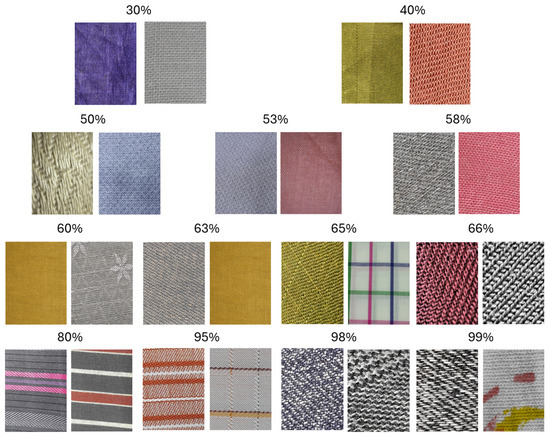
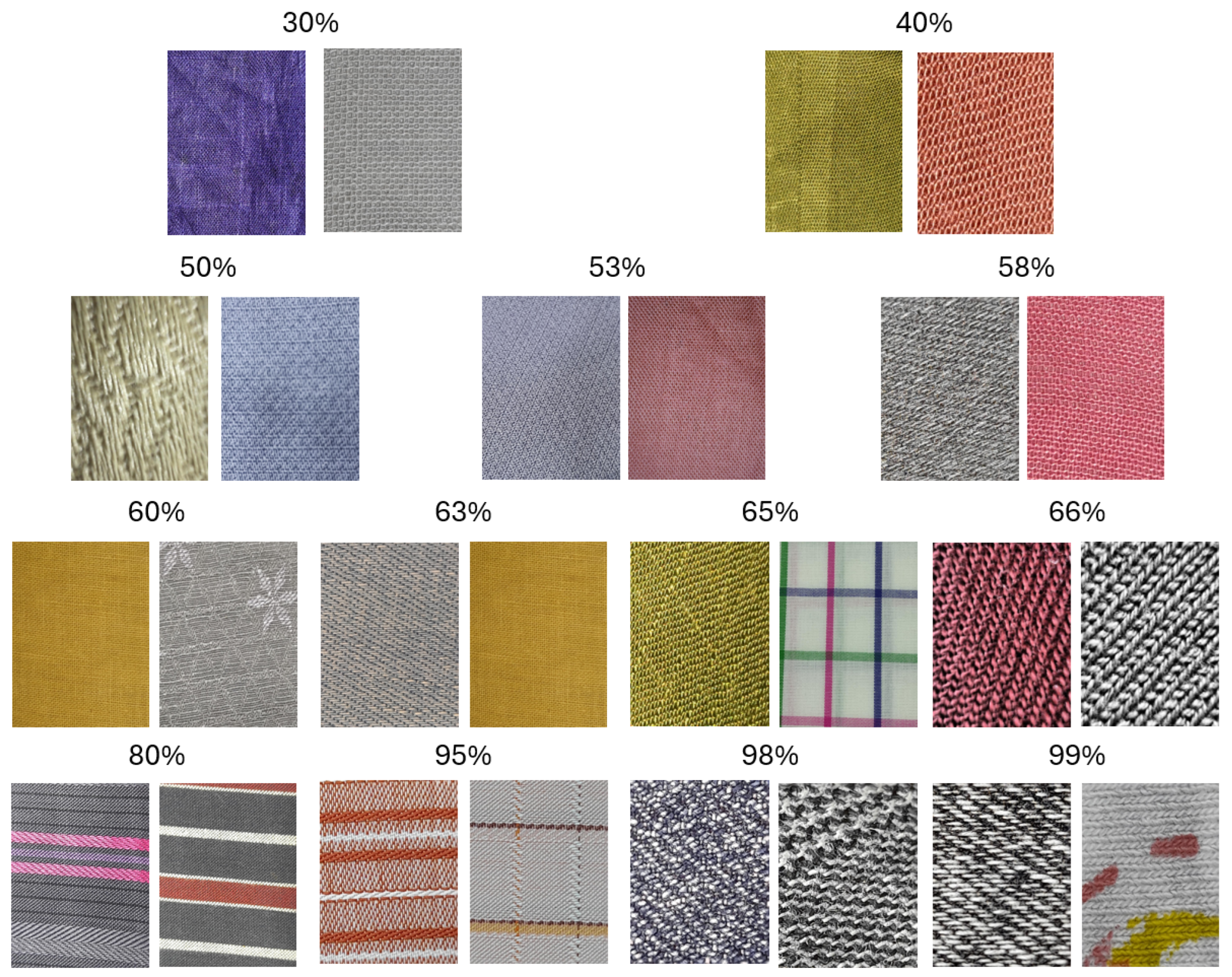
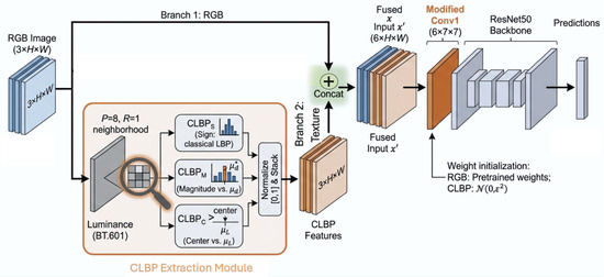
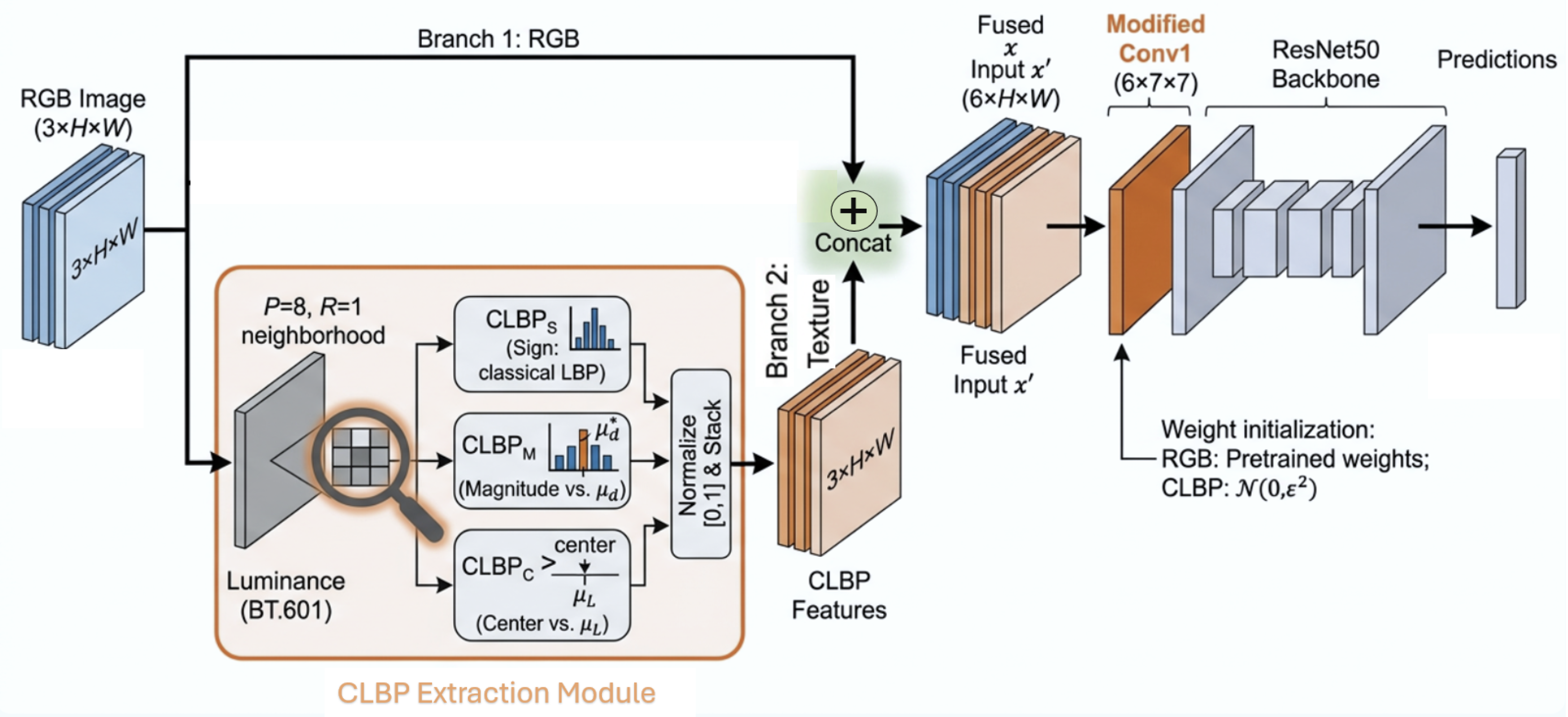
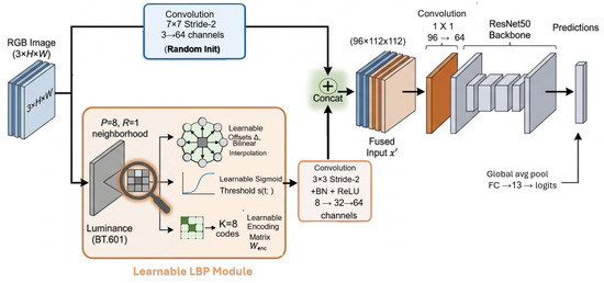
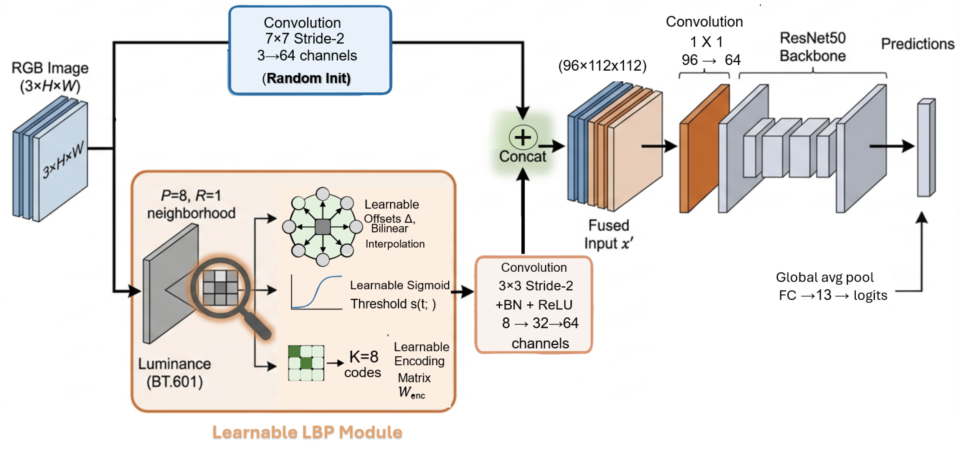
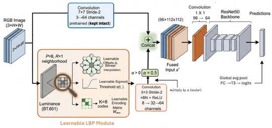
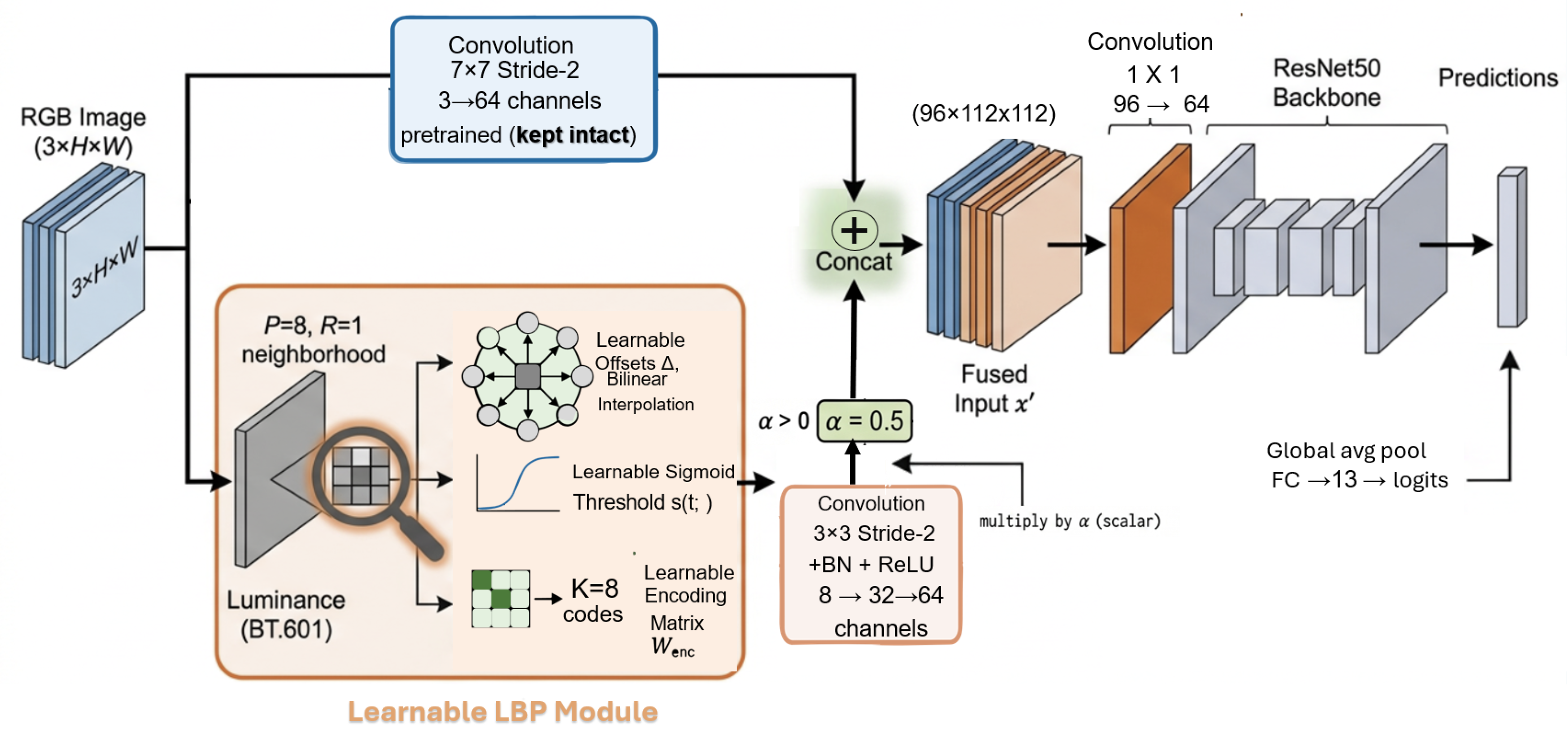
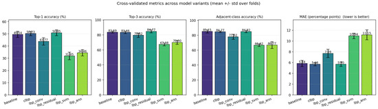
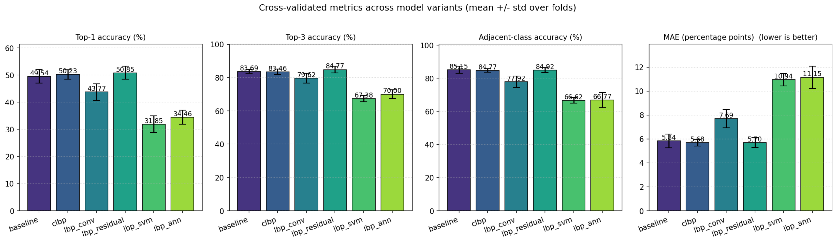
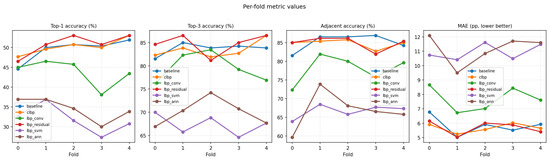
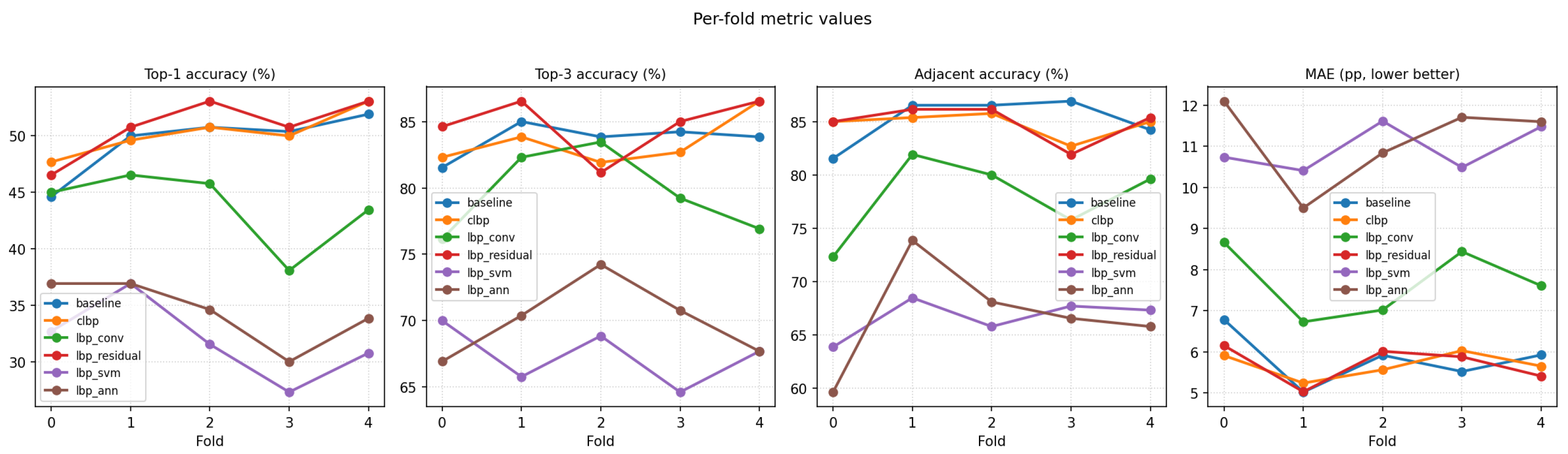
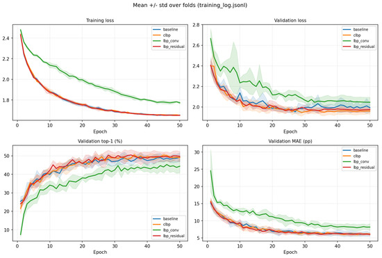
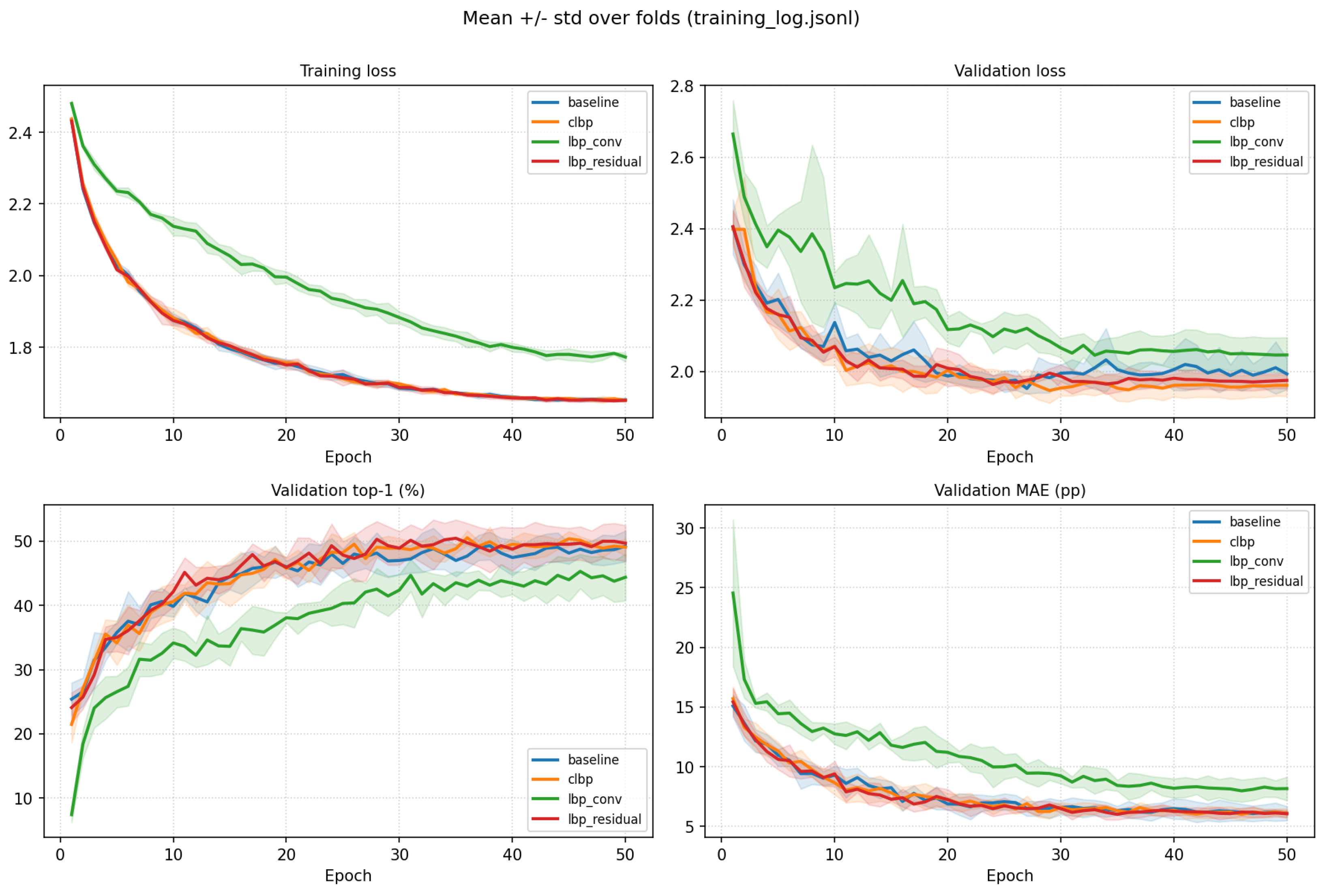
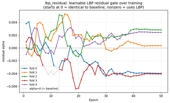
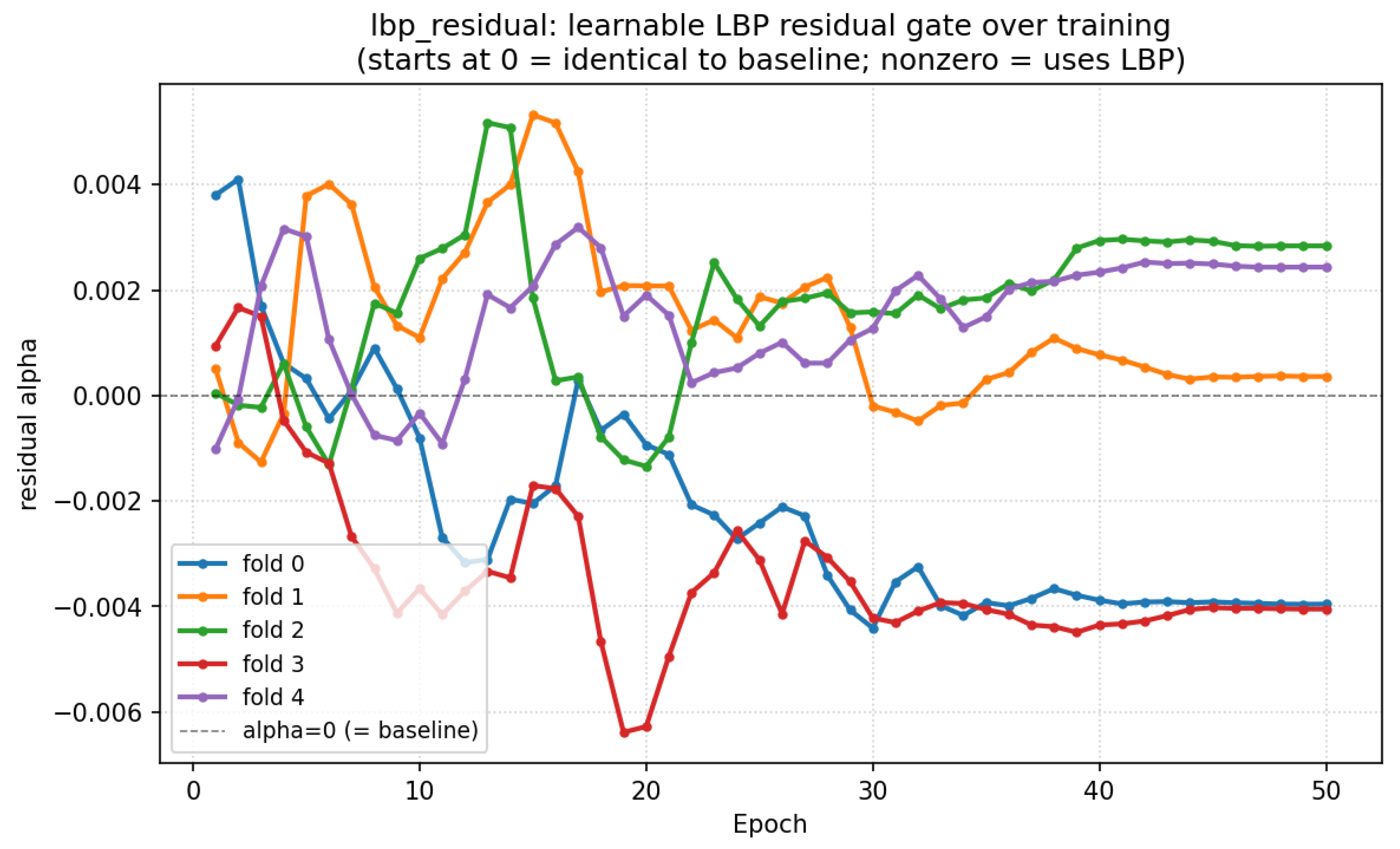
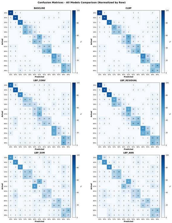
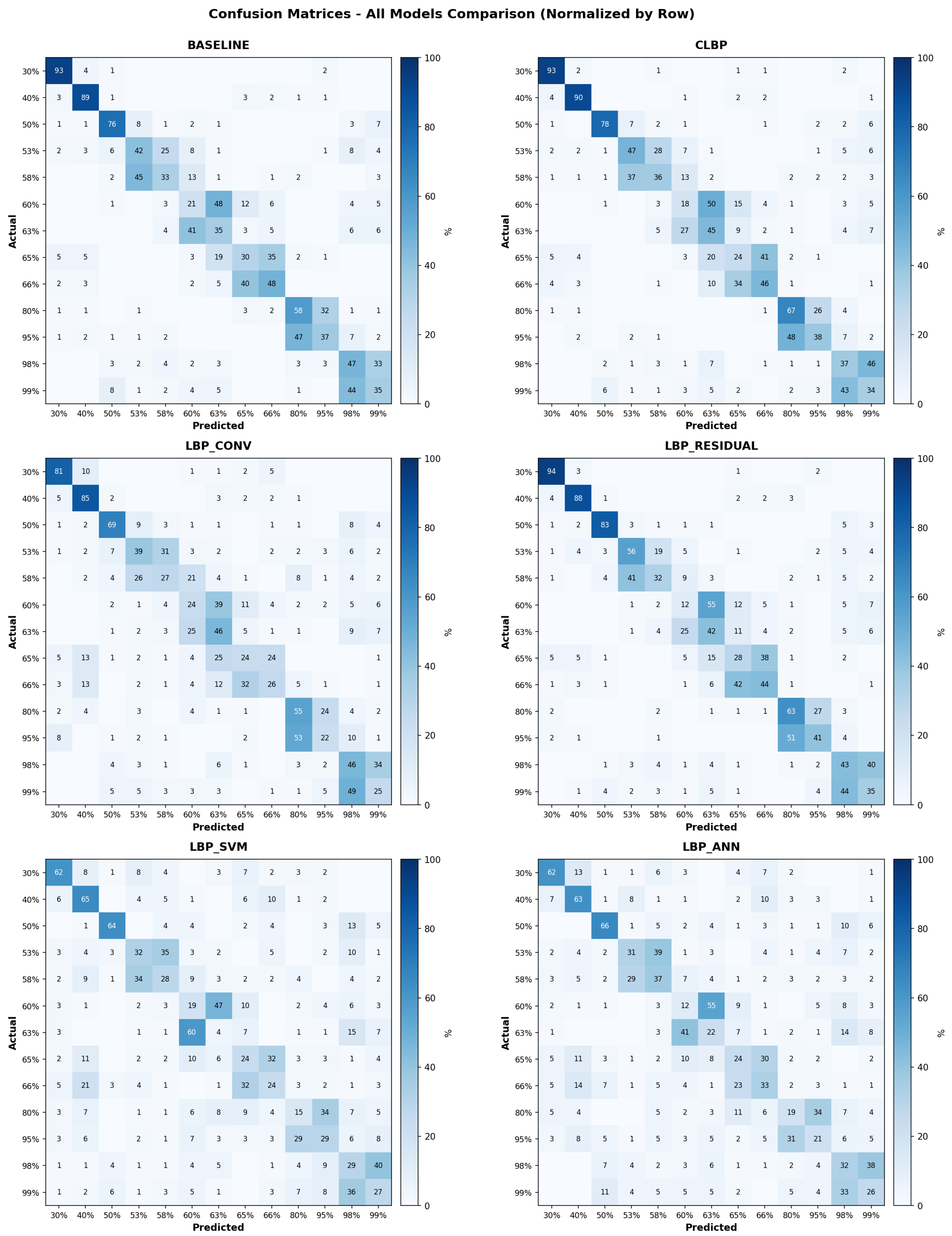
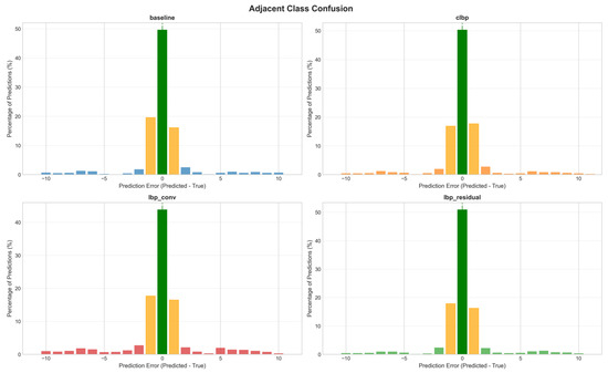
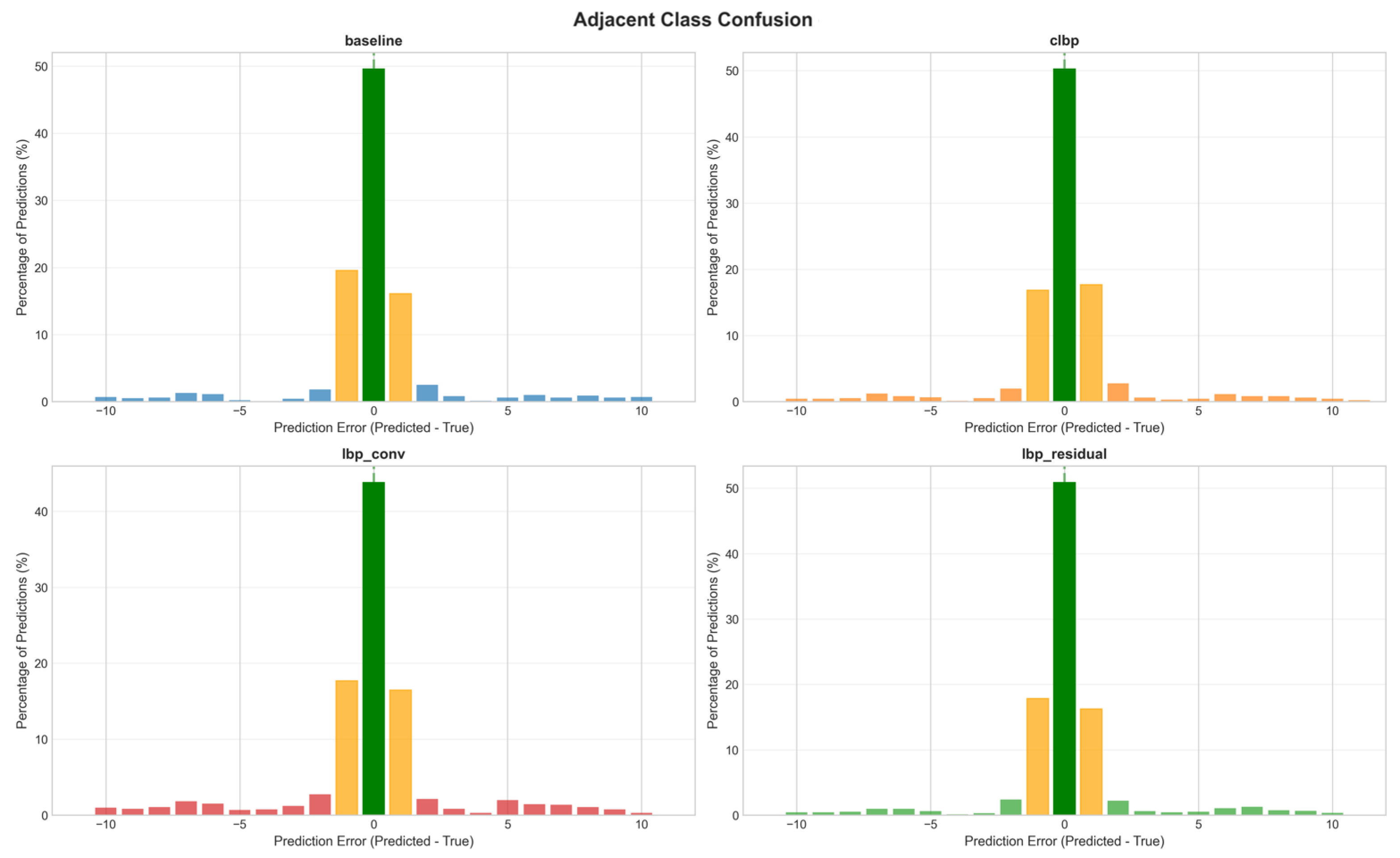

Disclaimer/Publisher’s Note: The statements, opinions and data contained in all publications are solely those of the individual author(s) and contributor(s) and not of MDPI and/or the editor(s). MDPI and/or the editor(s) disclaim responsibility for any injury to people or property resulting from any ideas, methods, instructions or products referred to in the content. |
© 2026 by the author. Licensee MDPI, Basel, Switzerland. This article is an open access article distributed under the terms and conditions of the Creative Commons Attribution (CC BY) license.