Employing Different Precipitation Products to Estimate Soil Loss and Sediment Yield: Application in the Zagros Mountains (Iraq–Iran)

Abstract

Soil erosion is one of the most serious environmental concerns of our time, leading to land degradation, agricultural inefficiency, reservoir siltation, and ecological imbalance. Thus, a thorough assessment of soil erosion is crucial whilst developing and implementing any conservation strategies and measures. In this context, the present research aims to estimate Soil Loss (SL) and Sediment Yield (SY) in the Chami Qeshan Watershed (CQW) between Iraq and Iran using the integrated application of the Revised Universal Soil Loss Equation (RUSLE) and Sediment Delivery Ratio (SDR) techniques. In addition to rain gauge observations, three satellite-derived precipitation datasets were applied for calculating the rainfall–runoff erosivity (R) variable of RUSLE, namely the Climate Hazards Group InfraRed Precipitation with Stations (CHIRPS), the Modern-Era Retrospective Analysis for Research and Applications, version 2 (MERRA-2), and the Tropical Rainfall Measuring Mission (TRMM). We also considered four other key factors for predicting soil erosion: soil erodibility (K), slope length and steepness (LS), cover management (C), and conservation practice (P). Ultimately, we used the Pearson correlation to statistically evaluate relationships between input variables and soil erosion outcomes. Results revealed substantial differences among the implemented products, where CHIRPS provided the best reproduction of annual precipitation. Likewise, the CHIRPS-based RUSLE-SDR model reproduced the closest mean soil loss of 12.18 t·ha⁻¹·yr⁻¹ and total outlet sediment yield of 51,826 t·yr⁻¹ to the corresponding gauge-driven model estimates. The correlation analysis found moderate associations between modeled soil loss estimates and LS (r = 0.56–0.57), C (r = 0.50–0.61), and P (r = 0.48–0.63) variables. Given the direct influence of precipitation products on rainfall erosivity and RUSLE–SDR estimates, native-resolution sensitivity analyses and alternative interpolation schemes are recommended to assess result robustness.

1. Introduction

Erosion is the mechanism by which rocks and soil on Earth’s surface are transported by exogenous forces and redeposited in different zones. This natural phenomenon is caused by the continual action of erosive factors: water, wind, ice, snow, animals, plants, and anthropogenic activities [1]. Globally, approximately 1094 million hectares of land are adversely affected by soil erosion due to hydrological processes, and 224 million hectares of that land are beyond reclamation [2]. The Food and Agriculture Organization (FAO) estimates that water erosion causes the loss of over 24 billion tons of fertile soil, a significant non-renewable natural resource, each year worldwide [3]. As a whole, soil erosion leads to on-site and off-site complexities. The loss of arable land, desertification, and subsequent economic detriments are the principal examples of on-site effects. Off-site repercussions of erosion, which typically emerge distant from the erosion site, include contaminating and clogging waterways, declining lake volume, deteriorating water quality, widening floodplains, diminishing aquatic life, inducing landslides, and sediment-related problems with water management structures. The primary off-site consequence of soil erosion is likely sediment yield to river systems and, ultimately, to reservoirs, resulting in reduced water storage capacity [4,5]. Therefore, the initial phase in resolving these issues is to quantify soil loss and sediment yield at the watershed scale.

Conventional techniques for estimating soil erosion include field surveys with experimental plots. This approach can produce reliable assessments; nevertheless, it is prohibitively expensive and laborious when investigating large domains. Thus, researchers introduced and implemented several empirical and physical models for evaluating soil erosion in published works, such as the Water Erosion Prediction Project (WEPP) [6,7,8], the European Soil Erosion Model (EUROSEM) [9], the Soil and Water Assessment Tool (SWAT) [10], the Sediment Delivery Distributed (SEDD) [11], the Universal Soil Loss Equation (USLE) [12], and the Revised USLE (RUSLE) [13]. The latter has been widely used worldwide and integrated with Geographic Information Systems (GISs) and satellite-derived thematic layers across different climate regions to efficiently and inexpensively estimate soil loss at various basin scales [14,15]. Rainfall–runoff erosivity (R), conservation practice (P), soil erodibility (K), cover management (C), and slope length and steepness (LS) are the five parameters that together make up the RUSLE model [16].

In situ precipitation measurements are unquestionably considered the most accurate and reliable; nonetheless, these ground observations have limited spatial coverage, short record periods, and missing values, particularly in remote mountainous regions. Most significantly, researchers consistently struggle to access such representative input data straightforwardly. The good news is that radar, satellite-derived, and reanalysis products, which differ in scale and coverage, are currently used as alternative sources of precipitation input for water-related applications [17]. In addition to measured precipitation data, this study utilized and tested three different precipitation products for calculating the R variable of the RUSLE model, namely the Climate Hazards Group InfraRed Precipitation with Stations (CHIRPS) [18], the Modern-Era Retrospective Analysis for Research and Applications, Version 2 (MERRA-2) [19], and the Tropical Rainfall Measuring Mission (TRMM) [20]. CHIRPS provides daily, pentadal, and monthly precipitation data with a spatial resolution of 0.05° for the years 1981 to the present, spanning the region between 50° S and 50° N. It was developed for the benefit of the Famine Early Warning Systems Network of the United States Agency for International Development. MERRA-2 is the most recent publicly released atmospheric reanalysis dataset from the National Aeronautics and Space Administration (NASA). It delivers observation-corrected precipitation estimates (i.e., PRECTOTCOR) with a horizontal resolution of 0.50° × 0.625° and a temporal resolution of 1 h, covering the period from 1980 onward. TRMM was established as a result of collaboration between NASA and the Japan Aerospace Exploration Agency (JAXA) to monitor and inspect precipitation in tropical and subtropical regions. The TRMM satellite has been operating since 1998 with a geographical resolution of 0.25° and a daily temporal resolution ranging from 50° S to 50° N. The aforementioned precipitation products have been applied and verified in numerous climatological and hydrological assessment studies [21,22,23,24,25].

Globally, many studies examined the applicability of satellite-based precipitation products for calculating the rainfall–runoff erosivity factor of RUSLE, such as [26], which implemented the high-frequency GPM-IMERG precipitation data to spatiotemporally assess rainfall erosivity in the Ecuadorian Andes and surrounding region using RUSLE. The evaluation findings showed great variability among the Ecuadorian basins; nevertheless, a frequent underestimation was observed. Another study [27] applied GPM-IMERG, PERSIANN-CDR, and TRMM 3B42 in a subtropical basin in China for estimating and mapping rainfall erosivity. The analysis revealed that the precision of estimates from GPM-IMERG was higher than that from TRMM 3B42, whereas PERSIANN-CDR overestimated light rainfall erosivity but underestimated heavy rainfall erosivity. A pertinent study [28] evaluated the ability of seven satellite-based precipitation products, including CHIRPS, IMERG, TRMM, ERA5, GLDAS, and PERSIANN-CDR, along with observed rain gauge data, to represent rainfall patterns and support R-factor estimation in the RUSLE framework in the Tungabhadra River Basin (TRB), India. Results showed that CHIRPS and IMERG displayed relatively smooth and continuous patterns, while PERSIANN-CDR and TRMM exhibited fragmented rainfall zones. ERA5 and GLDAS demonstrated consistent but moderate values across the basin.

Alongside, several international studies stated the significance of integrating the Index of Connectivity (IC) with RUSLE and the Sediment Delivery Ratio (SDR) approach to determine sediment dynamics. A published study [29] tested the combined RUSLE-IC-SDR method to estimate Sediment Yield (SY) and investigate the spatiotemporal variation in soil erosion rates and sediment connectivity in the Mediterranean Rogativa Catchment in southeast Spain. The study found the RUSLE-IC-SDR scheme effective in outlining the sources and hotspots on the hillslopes of an intricate Mediterranean catchment. A relevant research [30] proposed the integrated methodology of RUSLE, IC, and SDR to visually assess the spatiotemporal characteristics of erosion and sediment yield processes in the Yanhe Watershed in China with large-scale ecological restoration from 1985 to 2020 and to recognize the covariation between sediment connectivity and erosion in subbasins. The study concluded that the employed methods and acquired results provide ideas for separately defining both erosion and connectivity and quantifying a bivariate erosion–connectivity classification, which can be easily viewed on a scatterplot. Another investigation [31] estimated the sediment delivery ratio using the RUSLE-IC-SDR technique in a complicated landscape in Australia. The findings revealed that the RUSLE-IC-SDR technique can evaluate the entire sediment budget as well as the effects of rainfall, geomorphology, and vegetation cover on a complex landscape.

On a regional scale, numerous investigations have been conducted in the Zagros province and neighboring territories to quantify soil loss [32,33,34,35]. For instance, a study [36] integrated RUSLE with the SDR technique to calculate annual SL and sedimentation rates at the Darbandikhan Reservoir (DRR), using a set of scenarios. The research outcomes were validated using a bathymetric field survey of the considered artificial lake. Six out of the ninety scenarios analyzed had errors of less than 20%; scenario number 18 achieved optimal estimation, with an error of <1% and Reservoir Sedimentation (RSed) of 0.46458 km³·yr⁻¹. Another study [37] compared multiple RUSLE-SDR models for assessing RSed at Dukan Reservoir (DUR). The research employed three observed datasets (i.e., two bathymetric and one topographic map) to verify the findings. The annual RSed rate of DUR ranges from 0.0034 km³·y⁻¹ to 0.0027 km³·y⁻¹ from 1959 to 2023. Among the most substantial results were that GPM outperformed TRMM in computing the R factor and that one-third of the reservoir capacity is currently lost owing to sedimentation. A relevant investigation [38] was recently carried out to establish the soil loss tolerance limit and sediment yield in the Kanarwe River Basin (KRB). The findings revealed that the SL and SY rates range from 0.1 to 58.1 t·ha⁻¹·yr⁻¹ and from 0.1 to 29 t·ha⁻¹·yr⁻¹, respectively. In addition, none of the RUSLE input factors demonstrated a significant correlation greater than 0.5 with soil erosion outcomes. These existing studies have not comprehensively quantified soil loss and sediment yield for the entire Chami Qeshan Watershed (CQW), an important transboundary watershed between Iraq and Iran. As a result, there is a substantial gap in the literature that requires additional research.

The current study hypothesizes that if the precipitation input differs within a certain basin, those differences will most likely be manifested in the rainfall–runoff erosivity factor as well as the gross quantity of eroded soil and sediment outputs. The specific objectives of this research are to: (1) evaluate the reliability of CHIRPS, MERRA-2, and TRMM compared to rain gauge measurements as a driving force for calculating the R variable, (2) estimate soil loss in CQW based on four precipitation inputs, (3) predict sediment yield at the basin outlet, and (4) identify the most significant variables associated with soil erosion. The work presented herein provides one of the first investigations into how observed and satellite-derived precipitation datasets could affect SL and SY estimations in the data-scarce CQW. Therefore, the findings will assist in regulating and implementing erosion control measures and sustainable water management strategies in the region.

2. Materials and Methods

2.1. Study Area

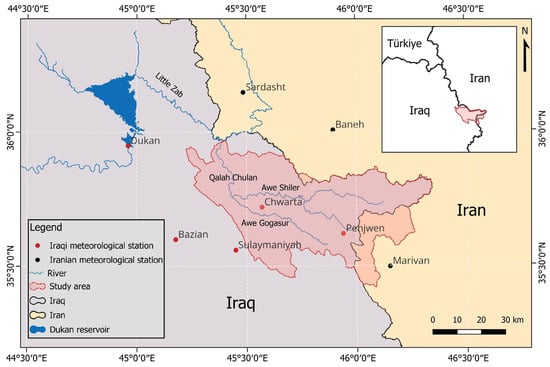
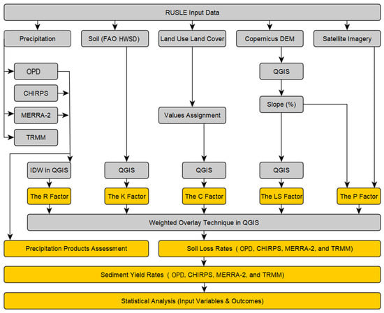
The Chami Qeshan Watershed, incorrectly identified as the Hami Qeshan Valley in an earlier study [39], is the largest subbasin of the Little Zab River Basin (LZRB) within the Kurdistan Region, located in the far northeast of Iraq, northwest of Iran [40]. It is positioned between latitudes 35°25′51′′ N and 35°57′56′′ N and longitudes 45°13′32′′ E and 46°20′57′′ E, predominantly in the Iraqi Sulaymaniyah Governorate (Figure 1). Approximately 3000 km² constitute the research territory, of which about 87% is situated in Iraq and the remaining 13% in Iran. CQW has slopes that range from flat to 76 degrees and elevations between 632 and 2755 m above sea level. As the region of interest lies within the Zagros orogenic belt, it is characterized by rugged topography and diverse lithostratigraphic units. In addition, CQW is considered a significant agricultural province in terms of freshwater resources and farming output (e.g., barley, wheat, pomegranates, grapes, pistachios, and walnuts) [41].

Figure 1. Geographical location of the Chami Qeshan Watershed, Iraq–Iran, and Dukan reservoir.

Hot, dry summers and wet, humid winters define the climate of CQW, which also exhibits significant seasonal variations in temperature, precipitation, and evapotranspiration. The average annual precipitation in the studied area from 2004 to 2018 ranged from 674 mm to 1057 mm. The months of October through May receive the most precipitation; January had the highest average monthly precipitation, measuring 207 mm. Likewise, the average monthly temperature ranged from 27.9 °C in July to −0.5 °C in January. Awe Gogasur and Awe Shiler Streams meet to produce the sixth-order Qalah Chulan River (QCR) in the area of interest. Furthermore, QCR joins the Little Zab River near Avcourta village, flowing from east to northwest. These waterways receive nearly all of their nourishment from rain, snowmelt, and springs, resulting in their discharge peaking in the spring and gradually diminishing from June to September [40].

2.2. Data Description

The in situ meteorological data, encompassing daily precipitation and temperature, were collected from two sources: the Ministry of Agriculture and Water Resources (MAWR) of the Iraqi Kurdistan Region and the Iranian Meteorological Organization (IMO), covering the period from 2004 to 2018 (Table 1). The missing values in observed meteorological records were filled with data from the nearest weather station before further evaluation. These data were first utilized to describe the climate of the investigated watershed. The daily precipitation measurements were aggregated to an annual scale, and after that, the mean was determined to calculate the rainfall–runoff erosivity factor. It is pertinent to note that the corresponding author attempted to gather further observed meteorological measurements, spanning 2019–2025; however, the ongoing war and sanctions on Iran made contact with the IMO futile. In addition, this study employed three satellite-derived precipitation datasets to determine the R factor: CHIRPS, MERRA-2, and TRMM. We downloaded CHIRPS daily precipitation data [42] from the World Weather for Water Data Service (W3S) webpage (https://www.uoguelph.ca/watershed/w3s, accessed on 4 October 2025) using defined rectangle coordinates. Bias-corrected daily MERRA-2 precipitation measurements [19] were acquired from the NASA POWER portal (https://power.larc.nasa.gov/data-access-viewer/, accessed on 5 October 2025) utilizing a point-based download technique. Both CHIRPS (spatial resolution: 0.05°) and MERRA-2 (horizontal resolution: 0.50° × 0.625°) were obtained in CSV format, covering the research period. Lastly, the daily TRMM 3B42-V7 dataset [22], with a pixel resolution of 0.25°, was gathered from the NASA GIOVANNI website (https://giovanni.gsfc.nasa.gov/giovanni/, accessed 23 October 2025). Because CHIRPS includes gauge observations, the CHIRPS v2 monthly station-use diagnostics for 2004–2018 were examined to evaluate the independence of the observational reference dataset. Based on coordinate matching with a 15 km tolerance, none of the eight meteorological stations used in this investigation were identified as being included in the final CHIRPS product. Aside from TRMM, which was obtained at an annual time scale, CHIRPS and MERRA-2 were first aggregated from daily to annual scale for precipitation reliability assessment. Then, the mean annual values of all products were determined for the calculation of the R factor. It is crucial to point out that the coordinates of the eight ground observations were considered while downloading the satellite-derived precipitation products.

Table 1. Meteorological station characteristics in and adjacent to CQW during the research period.

Station	Latitude	Longitude	Elevation (m)	Min AP (mm)	Max AP (mm)	Source
Baneh	36.0066	45.8955	1600	441	1059	IMO
Bazian	35.5986	45.1369	816	260	1095	MAWR
Chwarta	35.7200	45.5661	1128	455	1201	MAWR
Dukan	35.9500	44.9600	488	292	1018	MAWR
Marivan	35.4969	46.1514	1287	505	1296	IMO
Penjwen	35.6233	45.9433	1279	544	1706	MAWR
Sardasht	36.1483	45.4858	1557	550	1233	IMO
Sulaymaniyah	35.5567	45.4531	890	381	1234	MAWR

AP—annual precipitation in millimeters (mm); Min—minimum; Max—maximum; m—meter.

The OpenTopography portal (https://opentopography.org/, accessed 22 July 2022) provided the Copernicus Digital Elevation Model (CDEM), which has a pixel resolution of 30 m [43]. The CDEM has been used to establish the watershed boundary, subwatershed delineation, drainage network, slope length–steepness parameter, and slope map in degrees to determine the soil conservation practice variable. We developed the soil erodibility layer using the Harmonized World Soil Database (HWSD) at approximately 852 m spatial resolution [44]. The Land Use Land Cover (LULC) map used to generate the cover management variable was provided by the Iraq Geological Survey (GEOSURV) [45]. After being reprojected to zone 38 north of the Universal Transverse Mercator (UTM) in QGIS version 3.44.3, all digital maps were resampled at a spatial resolution of 30 m. It is important to declare that the satellite-based precipitation products were resampled to the 30 m computational grid required for integrating precipitation-derived R with the other RUSLE–SDR spatial factors; this procedure does not imply that the precipitation products provide spatial information at a 30 m resolution.

2.3. Conceptual Framework

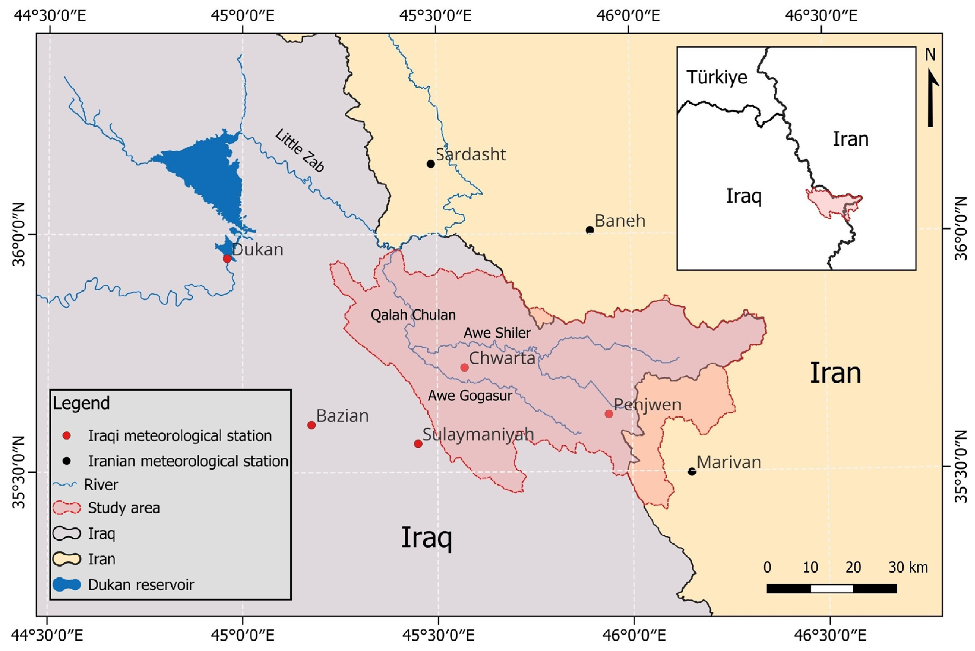
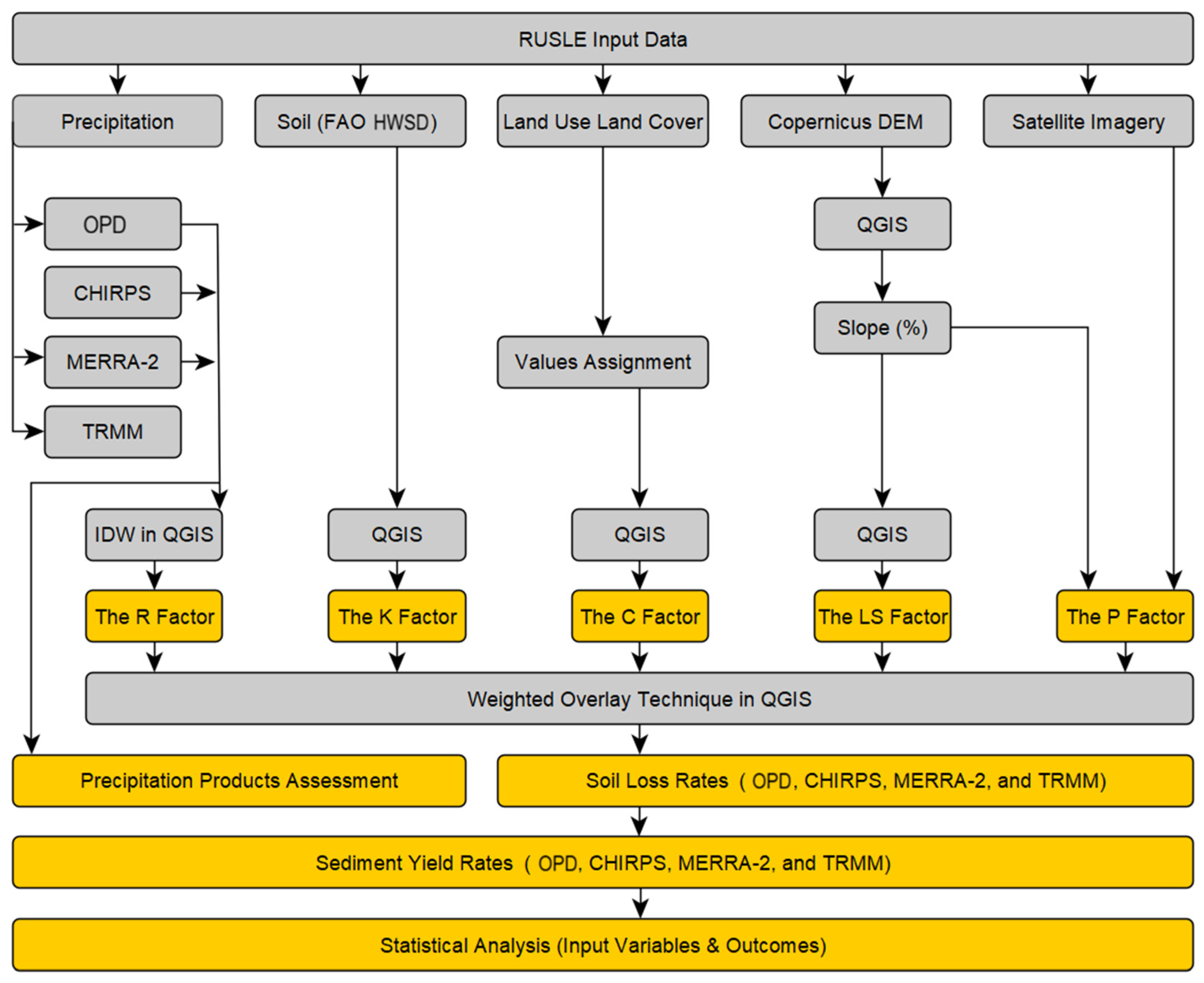
This study utilized four precipitation datasets, the FAO HWSD soil map, Copernicus DEM, a 2014 land use and land cover thematic layer, and satellite imagery within the QGIS environment to quantify SL and SY in the Chami Qeshan Watershed using the RUSLE and SDR techniques, as shown in Figure 2, which was created using the yEd software (version 3.25.1). The methodology consists of nine essential steps: (1) calculating the rainfall–runoff erosivity (R) factor using multiple precipitation products, specifically Observed Precipitation Data (OPD), CHIRPS, MERRA-2, and TRMM; (2) deriving the soil erodibility (K) factor based on soil texture (percentages of sand, silt, and clay) and organic carbon ratio from the FAO HWSD, and then applying them to a set of mathematical formulas; (3) integrating the LULC classes and values attained from the literature to create the cover management (C) factor; (4) employing the CDEM data to extract the slope length and steepness (LS) factor; (5) extracting the slope map as a percentage from CDEM and combining it with information obtained from satellite imagery to generate the conservation practice (P) factor; (6) assessing the performance of the applied precipitation products by means of statistical metrics; (7) applying the RUSLE model in QGIS to map and estimate soil loss rate; (8) predicting total sediment yield at the basin outlet; and (9) analyzing the association between input variables and soil erosion outcomes. All variables were processed in the QGIS environment (version 3.34.11). Section 2.4, Section 2.5 and Section 2.6 provide a comprehensive explanation of each stage.

Figure 2. Conceptual framework implemented in the current investigation.

2.4. The RUSLE Model

Renard and colleagues at the United States Department of Agriculture presented the RUSLE model in 1991 [15] to calculate water-induced soil loss in erosion-prone areas [13]. With numerous studies and comparable results, RUSLE has demonstrated its applicability to almost every condition and location on Earth [46]. Accordingly, the RUSLE model was selected to estimate the average annual soil loss in the Chami Qeshan Watershed using Equation (1) [13]:

A = R × K × LS × C × P

(1)

where A denotes the calculated average annual soil loss (t·ha⁻¹·yr⁻¹), R signifies the rainfall–runoff erosivity factor (MJ·mm·ha⁻¹·hr⁻¹·yr⁻¹), K refers to the soil erodibility factor (t·ha·hr·ha⁻¹·MJ⁻¹·mm⁻¹), LS represents the slope length–steepness factor (dimensionless), C symbolizes the land cover management factor (dimensionless), and lastly P designates the soil conservation practice factor (dimensionless). The following subsections provide a detailed description of the factors outlined above.

2.4.1. Rainfall–Runoff Erosivity (R)

The R factor characterizes the effect of rainfall and indicates the quantity and pace of runoff that precipitation episodes are anticipated to cause soil erosion ultimately. It is feasible to compute the rainfall erosivity factor for a single storm as a function of rainfall intensity, volume, and duration. Nonetheless, additional techniques exist to compute it from mean annual precipitation in data-scarce regions [47]. Since the investigated basin is poorly gauged, positioned between two countries, and most meteorological stations were installed after the Iraq War in 2003, the present study, in addition to observed precipitation measurements, employed three satellite-based precipitation products to examine their performance and competence in the Zagros Mountains range for soil loss calculations. In other words, we produced four rainfall–runoff erosivity thematic layers for the RUSLE model relying on four precipitation datasets: OPD, CHIRPS, MERRA-2, and TRMM. Basically, the R factor is computed from long-term precipitation data using a variety of methods [14]. For this study, the rainfall–runoff erosivity factor was derived following Equation (2), which has been implemented in the same climate conditions and region (i.e., the Khabur River Basin between Iraq and Türkiye) [35]:

R = 81.5 + (0.38 × MAP)

(2)

where R implies the rainfall–runoff erosivity factor (MJ·mm·ha⁻¹·hr⁻¹·yr⁻¹) and MAP indicates mean annual precipitation in mm (2004–2018). The Inverse Distance Weighting (IDW) technique was applied herein to interpolate the mean annual precipitation data extracted from OPD, CHIRPS, and MERRA-2. At the same time, TRMM was first reprojected from a 0.25° × 0.25–pixel resolution to UTM zone 38 north, vectorized as points, and interpolated using IDW. All precipitation maps were eventually resampled to a 30 m spatial resolution and used to calculate the R factor.

2.4.2. Soil Erodibility (K)

The K factor is an indicator of the inherent capability of soil particles to resist detachment and transport forces of rainfall and runoff [47]. Theoretically, the K value ranges from 0 to 1, where 0 denotes the least degree of soil susceptibility to erosion, and 1 denotes the greatest soil vulnerability to erosion [5]. Several variables play key roles in determining K values, including soil texture (i.e., sand, silt, and clay percentages), soil structure, coarse fragments, permeability, organic matter, slope, and other factors [36,48]. For this research, the HWSD dataset was used to acquire soil characteristics for calculating the K factor of RUSLE. Even though the reliability of HWSD varies per region due to the use of multiple dataset sources, a recent study [49] tested the accuracy of HWSD and found that the Mean Absolute Error (MAE) of sand, silt, clay, and organic matter is 17.65%, 6.44%, 14.26%, and 0.5%, respectively. The HWSD dataset is widely employed in regional and international studies relating to RUSLE estimation [50,51,52]. The K factor was calculated for CQW using Equation (3) [51,53,54], whereas M, OM, and SN are expressed in Equations (4) [12], (5) [55], and (6) [53], respectively, as follows:

$$K=\left[\left[0.2+0.3e^{\left[-0.0256m_{s\left(1-{\displaystyle \frac{m_{\mathit{silt}}}{100}}\right)}\right]}\right]\times {\left({\displaystyle \frac{m_{\mathit{silt}}}{{m_c+m}_{\mathit{silt}}}}\right)}^{0.3}\times \left[1-{\displaystyle \frac{0.25\mathit{OM}}{\mathit{OM}+e^{\left(3.72-2.9\mathit{OM}\right)}}}\right]\times \left[1-{\displaystyle \frac{0.7\mathit{SN}}{\mathit{SN}+e^{(22.9\mathit{SN}-5.51)}}}\right]\right]\times 0.1317$$

(3)

M = (m_silt + m_vfs) × (100 − m_c)

(4)

OM = 1.724 × OC

(5)

$$\mathit{SN}={\displaystyle \frac{1-m_{\mathit{sa}}}{100}}$$

(6)

where m_c, m_silt, m_s, and m_vfs refer to the clay, silt, sand, and very fine sand contents in percent, respectively. In addition, OM and OC represent soil organic matter and organic carbon contents in percent, respectively. In addition, s and p signify the soil structure class (Table A1 in Appendix A) and the permeability class (Table A2 in Appendix A), respectively [12,56]. For processing in the International System of Units, the K factor values were multiplied by 0.1317 [57].

2.4.3. Slope Length (L) and Slope Steepness (S)

The LS factor calculates the integrated impacts of slope length and steepness on soil erosion and is incorporated into the RUSLE model to account for topographic effects on soil loss [58]. Multiple equations have been proposed in the literature for calculating the slope length (L), such as [12,13,59]. For this study, Equations (7)–(9) presented by Moore and Burch [60] were employed to compute L. Consequently, the slope map in percent was derived and categorized into four classes: <1%, 1–3%, 3–5%, and ≥5%. Each slope class has its own constant m value, as shown in Equation (9). At the same time, the slope steepness (S) is calculated by means of three slope classes in percent: <9%, 9–18%, and ≥18% (Equation (10)) [61]. Equation (11) was ultimately applied to determine the LS factor [35].

$$L={\left({\displaystyle \frac{\mathsf{\lambda }}{22.12848}}\right)}^m$$

(7)

λ = FA × Ps

(8)

$$m=\left\{\begin{array}{cc}0.2& \hfill \theta <1\%\\ 0.3& \hfill 1\%\le \theta <3\%\\ 0.4& \hfill 3\% \le \theta <5\%\\ 0.5& \hfill \theta \ge 5\%\end{array}\right.$$

(9)

$$S=\left\{\begin{array}{cc}10.8\times \mathit{sin\theta }+0.03& \hfill \theta <9\%\\ 16.8\times \mathit{sin\theta }-0.05& \hfill 9\%\le \theta <18\%\\ 21.9\times \mathit{sin\theta }-0.96& \hfill \theta \ge 18\%\end{array}\right.$$

(10)

LS = L × S

(11)

where L stands for the slope length, S means the slope steepness, λ refers to the horizontal projection of slope length (m), m denotes a constant based on the value of slope gradient (Equation (9)), FA signifies stream flow accumulation, Ps indicates the pixel size of the DEM, and θ represents the slope gradient in percent.

2.4.4. Cover Management (C)

The C factor reflects the influence of plant cover, cropping, and land management practices on soil erosion rates. It is the proportion of soil loss from vegetated land to that from continuously fallow ground [47]. The LULC layer of CQW was obtained in shapefile format from GEOSURV. This map was created using 2014 Landsat 8 OLI data, where multiple image indices and supervised classification were applied via the maximum likelihood algorithm [45]. The accuracy of classification was evaluated for the used LULC thematic layer by comparing classification results with established data, where the LULC map achieved an overall classification accuracy of 81.7%, as revealed in Table 2. Based on several studies, the LULC classes were assigned C factor values varying between 0, indicating extremely high cover effects on soil erosion, and 0.5, implying no land cover, and the area was classified as barren land. The C values for this investigation have been established using the literature given in Table 3, corresponding to various land cover categories.

Table 2. Accuracy assessment of the LULC map of the study area [45].

LULC Units	Reference Totals (True)	Classified Totals (Predicted)	Number Correct	Producer’s Accuracy (%)	User’s Accuracy (%)
Urban and Built-Up Land	41	29	29	70.7	100.0
Natural Vegetation	26	24	19	73.1	79.2
Cropland and Pasture	40	36	35	87.5	97.2
Cultivated Land	37	37	26	94.6	74.3
Harvested Land	40	33	29	72.5	87.9
Burned Land	17	6	5	29.4	83.3
Igneous and/or Metamorphic Rocks	36	32	27	75.0	84.4
Carbonate Rocks	26	36	24	92.3	66.7
Clastic Rocks	47	54	46	97.9	85.2
Mixed Barren Land	132	151	121	91.7	80.1
Total	442	438	361
Overall Classification Accuracy (%) = 81.7
Overall Kappa Statistic = 0.783

Table 3. Assigned C values to the existing LULC categories in the investigated watershed.

LULC Type	LULC Description	C Factor	Reference
Agriculture	Lands used for perennial/annual crop cultivation	0.24	[47]
Bare Land	Lands with no greenery masses or building projects	0.50	[62]
Grassland	Lands chiefly covered with grasses	0.05	[47]
Settlement	Lands principally shielded by man-made structures	0	[5]
Shrubland	Vegetated lands dominated by shrubs	0.03	[5]

2.4.5. Conservation Practice (P)

The P factor describes the impact of contour tillage on water-induced soil erosion [13]. Put differently, it refers to the relationship between runoff-induced soil loss under specific conservation practices (i.e., contouring, terracing, and strip-cropping) and the corresponding loss up- and down-slope. Theoretically, P factor values range from 0 to 1, where 0 indicates highly effective erosion-resistance management strategies, and 1 indicates no man-made erosion-resistance actions [47,63,64]. For circumstances similar to those in CQW, the P factor is assessed based on the slope angle in percent and frequently applied conservation practices, where the information in the current study was gathered from satellite observations and found that strip-cropping is the most popular method of controlling soil erosion; the greenery mass values were then assigned in QGIS based on the classification of Shin [65] (Table 4), whereas terrains with no erosion control practices were assigned a p value of 1 [64].

Table 4. Linking between different soil conservation practices and slope categorization [47,63].

Slope (%)	Soil Conservation Practice (P Factor)
	Contouring	Strip-Cropping	Terracing
0–7	0.55	0.27	0.10
7–11.3	0.60	0.30	0.12
11.3–17.6	0.80	0.40	0.16
17.6–26.8	0.90	0.45	0.18
>26.8	1.00	0.50	0.20

2.5. Sediment Yield Estimation

Soil erosion occurs in three distinct stages: the detachment of soil particles, the movement of eroded materials by surface runoff, and the deposition of sediment particles. Nevertheless, RUSLE is unable to account for the transportation and deposition of eroded sediments; it merely predicts and quantifies soil loss. Accordingly, the concept of Sediment Delivery Ratio (SDR) can be combined with RUSLE to estimate sediment yield [2]. The SDR of a drainage basin is expressed as the ratio of SY at the basin outlet to overall erosion within a basin. This formulation allows for the spatial variability of gross sediment production in massive basins [3]. The SDR value ranges from 0 to 1, where 0 indicates no sediment delivery, and 1 represents full sediment delivery [66]. For this study, we applied the SDR model suggested by earlier research [67], which uses IC to estimate SDR (Equation (12)). The IC calculation depends on the average weighting factor $\left(\overline{W}\right)$ of the contributing area (Equation (13)), which can be influenced by the basin’s topography (i.e., topographic surface roughness) (RS; Equation (14)). The RS is substantial for calculating the $\overline{W}$, which is required to estimate SDR. The RS has been calculated using the connectivity index toolbox [68] following Equation (15).

$$\mathit{SDR}={\displaystyle \frac{{\mathit{SDR}}_{\mathit{max}}}{1+e^{\left(\frac{{\mathit{IC}}_0-{\mathit{IC}}_i}{k_b}\right)}}}$$

(12)

$${\mathit{IC}}_i={\mathit{log}}_{10}\left({\displaystyle \frac{D_{\mathit{up}}}{D_{\mathit{dn}}}}\right)={\mathit{log}}_{10}\left({\displaystyle \frac{\overline{W}\overline{S}\sqrt{A}}{\sum _i\frac{d_i}{W_i{S}_i}}}\right)$$

(13)

$$W_i=1-\left({\displaystyle \frac{\mathit{RS}}{{\mathit{RS}}_{\mathit{max}}}}\right)$$

(14)

$$\mathit{RS}=\sqrt{{\displaystyle \frac{{\displaystyle {\sum }_{i=1}^{{\mathit{mws}}^2}}{(x}_i-\overline{x}{)}^2}{{\mathit{mws}}^2}}}$$

(15)

where SDR and SDR_max stand for the sediment delivery ratio and the maximum theoretical value of SDR, respectively. SDR_max equals 0.8 [69,70]. The calibration parameters IC₀ and K_b are 0.5 and 2, respectively [71]. IC_i refers to the connectivity index for a specific pixel. The D_up and D_dn indicate the upslope and downslope components, respectively. $\overline{W}$ signifies the average weighting factor for the contributing area; A denotes the contributing area (m²); $\overline{S}$ symbolizes the average slope of the upslope contributing area (m/m). Moreover, d_i, W_i, and S_i stand for the flow path to the downstream main channel, the weighting factor, and the slope gradient for a specific pixel, respectively. RS means the topographic surface roughness. As well, mws represents the moving window size, which was suggested to be 5 × 5 by previous research [72]. Likewise, x_i denotes the value of the pixel located in the center of the moving window, and $\overline{x}$ symbolizes the mean of the pixel values within the moving window. Ultimately, the sediment yield was estimated through pixel-wise integration of the RUSLE-derived soil erosion and IC-based SDR layers. For each 30 m pixel, the estimated soil erosion rate (A_i in t·ha⁻¹·yr⁻¹) was multiplied by its corresponding dimensionless SDR value (SDR_i). Subsequently, total sediment yield at the watershed outlet (SY_outlet) was calculated as follows:

$${\mathit{SY}}_{\mathit{outlet}}=\left[{\sum }_{i=1}^n{A}_i\times {\mathit{SDR}}_i\right]\times a_i$$

(16)

where a_i stands for the pixel area (i.e., 0.09 ha for the 30 × 30 m pixel resolution) and n refers to the number of pixels within the watershed. Thus, the pixel-level sediment yield values were summed and multiplied by 0.09 ha to obtain the total outlet sediment yield in t yr⁻¹.

2.6. Statistical Metrics

This study essentially involved two assessment sections: (1) evaluating three different satellite-derived precipitation products compared to rain gauge observations on the annual scale using continuous statistical metrics—Coefficient of Determination (R²) and Root Mean Square ERROR (RMSE)—and (2) comprehending the relationship between input variables and modeled soil loss estimates throughout the Pearson correlation coefficient (r) matrix. R² describes the degree of agreement between measured and estimated precipitation values (Equation (17)). RMSE indicates the extent to which estimated values deviate from observed values in a regression analysis (Equation (18)) [17]. Additionally, Mean Absolute Percentage Error (MAPE), which is perhaps the most frequently utilized goodness-of-fit indicator between observed and predicted data (Equation (19)) [73], was used to determine the error percentage in the implemented IDW scheme. The Pearson Correlation Coefficient (r) [74] is one of the oldest and most extensively applied statistical measures for assessing relationships between variables. The r values theoretically vary from +1 to −1, with the signs indicating the direction and strength of a linear relationship between variables. Moreover, +1 signifies an ideal positive linear correlation among components, −1 implies an optimal negative linear connection, and zero values symbolize no linear relationship [75,76]. The r value is commonly used to quantify the degree of agreement between estimated precipitation data and rain gauge measurements (Equation (20)) [40]. According to [77], if the r value exceeds 0.7, the gridded product is treated as a trustworthy source of precipitation data. We used the OriginPro software (version 2026b) to perform the statistical analyses for this investigation.

$${\mathrm{R}}^2={\displaystyle \frac{\left[{\displaystyle {\sum }_{i=1}^n}(\mathit{Oi}-\overline{O})(\mathit{Ei}-\overline{E})\right.{]}^2}{{\displaystyle {\sum }_{i=1}^n}(\mathit{Oi}-\overline{O}{)}^2 {\displaystyle {\sum }_{i=1}^n}(\mathit{Ei}-\overline{E}{)}^2}}$$

(17)

$$\mathit{RMSE}=\sqrt{{\displaystyle \frac{{{\sum }_{i=1}^n(\mathit{Ei}-\mathit{Oi})}^2}{n}}}$$

(18)

$$\mathit{MAPE}={\displaystyle \frac{1}{n}}{\sum }_{i=1}^n{\displaystyle \frac{\left|\mathit{Ei}-\mathit{Oi}\right|}{\mathit{Oi}}}\ast 100$$

(19)

$$r={\displaystyle \frac{{\displaystyle {\sum }_{i=1}^n}\left(\mathit{Oi}-\overline{O}\right)\left(\mathit{Ei}-\overline{E}\right)}{\sqrt{{\displaystyle {\sum }_{i=1}^n}{\left(\mathit{Oi}-\overline{O}\right)}^2}\sqrt{{\displaystyle {\sum }_{i=1}^n}{\left(\mathit{Ei}-\overline{E}\right)}^2}}}$$

(20)

where n refers to the sample size, Oi describes observed data, Ei denotes estimated data, and the bar symbol implies the average.

3. Results

3.1. Evaluation of Precipitation Products and RUSLE Parameters

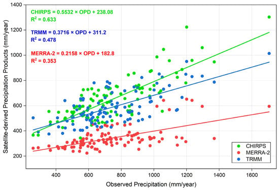
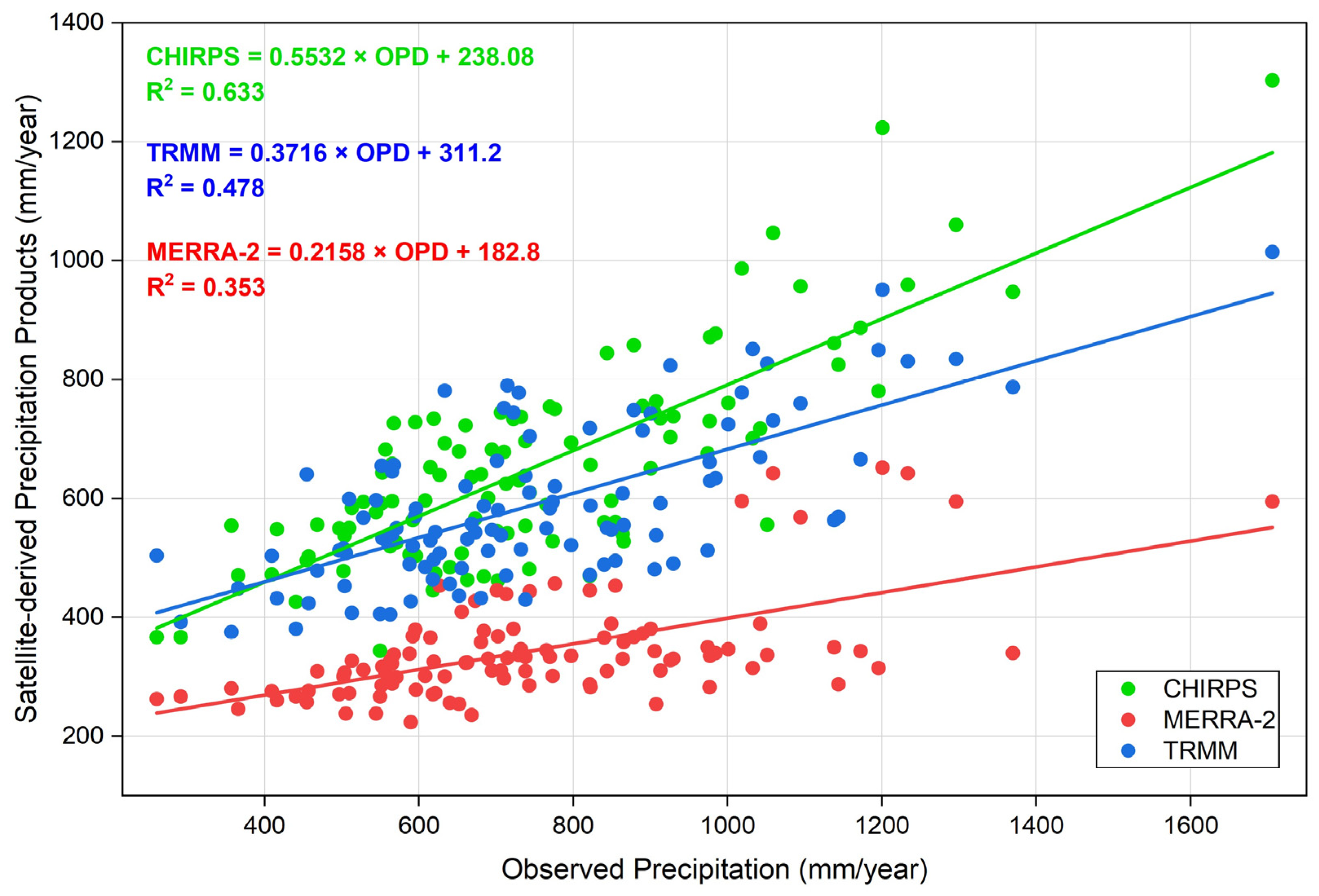
The comparison between annual precipitation from rain gauges and three satellite-derived precipitation products yielded distinct differences in their statistical performance. CHIRPS displayed the strongest positive linear relationship with observed precipitation, with a coefficient of determination (R² = 0.633), followed by TRMM (R² = 0.478) and MERRA-2 (R² = 0.353), as revealed in Figure 3. Likewise, the RMSE outcomes further supported this finding, with CHIRPS recording the lowest error (177.8 mm/year), followed by TRMM (240 mm/year) and MERRA-2 (452.1 mm/year). Overall, the integrated evaluation of R² and RMSE established CHIRPS as the best-performing product for reproducing observed annual precipitation variability, followed by TRMM and lastly MERRA-2 under the conditions of the current investigation. These results emphasize the significance of assessing satellite precipitation products against ground observations before selecting datasets for soil erosion and hydrological modelling applications.

Figure 3. Linear relationships between observed and satellite-derived annual precipitation data.

The capability of IDW was initially examined in the study region by means of leave-one-out IDW errors using the OPD reference. The IDW interpolation scheme achieved a MAPE of 7.7%, demonstrating relatively low average percentage deviations between the interpolated and observed precipitation values and, therefore, good predictive performance. This finding suggests that IDW provides a trustworthy depiction of precipitation spatial variability in the investigated basin.

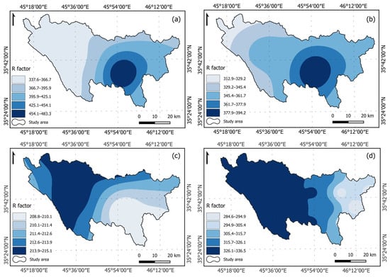
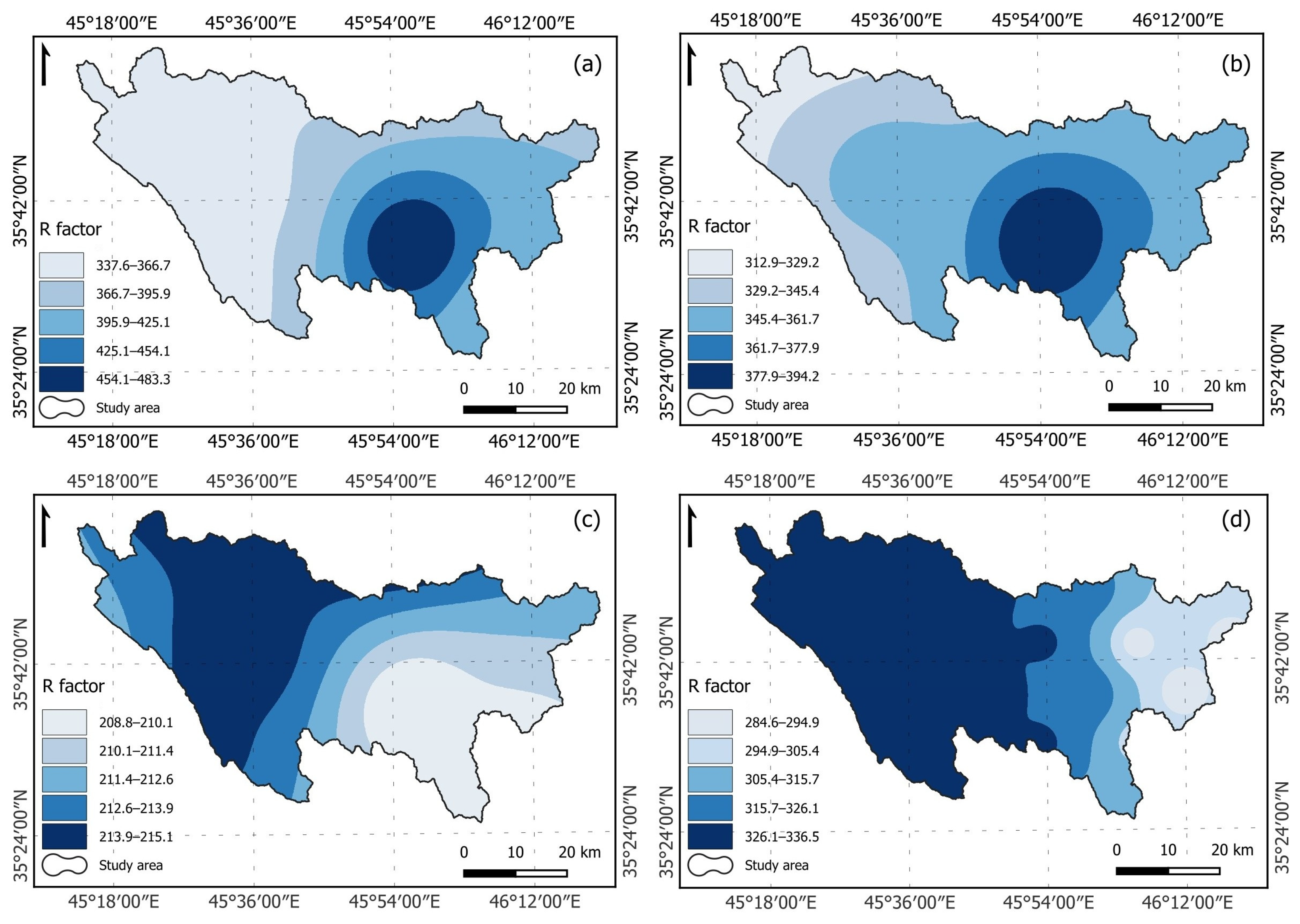
The mean annual precipitation values of all precipitation datasets were primarily determined in order to calculate the rainfall–runoff erosivity variable of RUSLE. These values were then interpolated using the IDW technique. The MAP measured at rain gauges inside and neighboring CQW ranged from 674 mm to 1057 mm. Likewise, the MAPs of CHIRPS, MERRA-2, and TRMM varied from 609 mm to 823 mm, 335 mm to 352 mm, and 534 mm to 671 mm, respectively. Even though all satellite-derived products underestimated the mean annual precipitation compared to rain gauge measurements, which served as the reference benchmark, CHIRPS performed the best with reasonable agreement with observations, followed by TRMM, which showed moderate variability, and MERRA-2 had the weakest performance. The R factor of RUSLE was calculated for this study utilizing Equation (2) and the above-mentioned precipitation datasets. Aside from OPD (R = 337.6–483.3 MJ·mm·ha⁻¹·hr⁻¹·yr⁻¹), the highest rainfall–runoff erosivity range of 312.9–394.2 MJ·mm·ha⁻¹·hr⁻¹·yr⁻¹ was reached using CHIRPS, followed by TRMM (R = 284.6–336.5 MJ·mm·ha⁻¹·hr⁻¹·yr⁻¹), and the lowest R range of 208.8–215.1 MJ·mm·ha⁻¹·hr⁻¹·yr⁻¹ was achieved based on MERRA-2, as illustrated in Figure 4.

Figure 4. Rainfall–runoff erosivity factor maps in MJ·mm·ha⁻¹·hr⁻¹·yr⁻¹ based on precipitation data derived from: (a) OPD, (b) CHIRPS, (c) MERRA-2, and (d) TRMM.

It is vital to state that CHIRPS not only indicated good skill in producing erosive precipitation but also had the closest spatial distribution to OPD-based R (Figure 4a,b). On the flip side, the spatial distribution patterns of MERRA-2 and TRMM (Figure 4c,d) appear in a way that contradicts the OPD-based R, in which the highest values are concentrated in the eastern part of CQW. Taken together, these findings suggest that MAP inconsistencies across the implemented datasets have undoubtedly been mirrored and propagated to the measured erosivity.

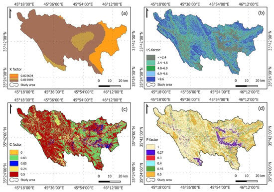
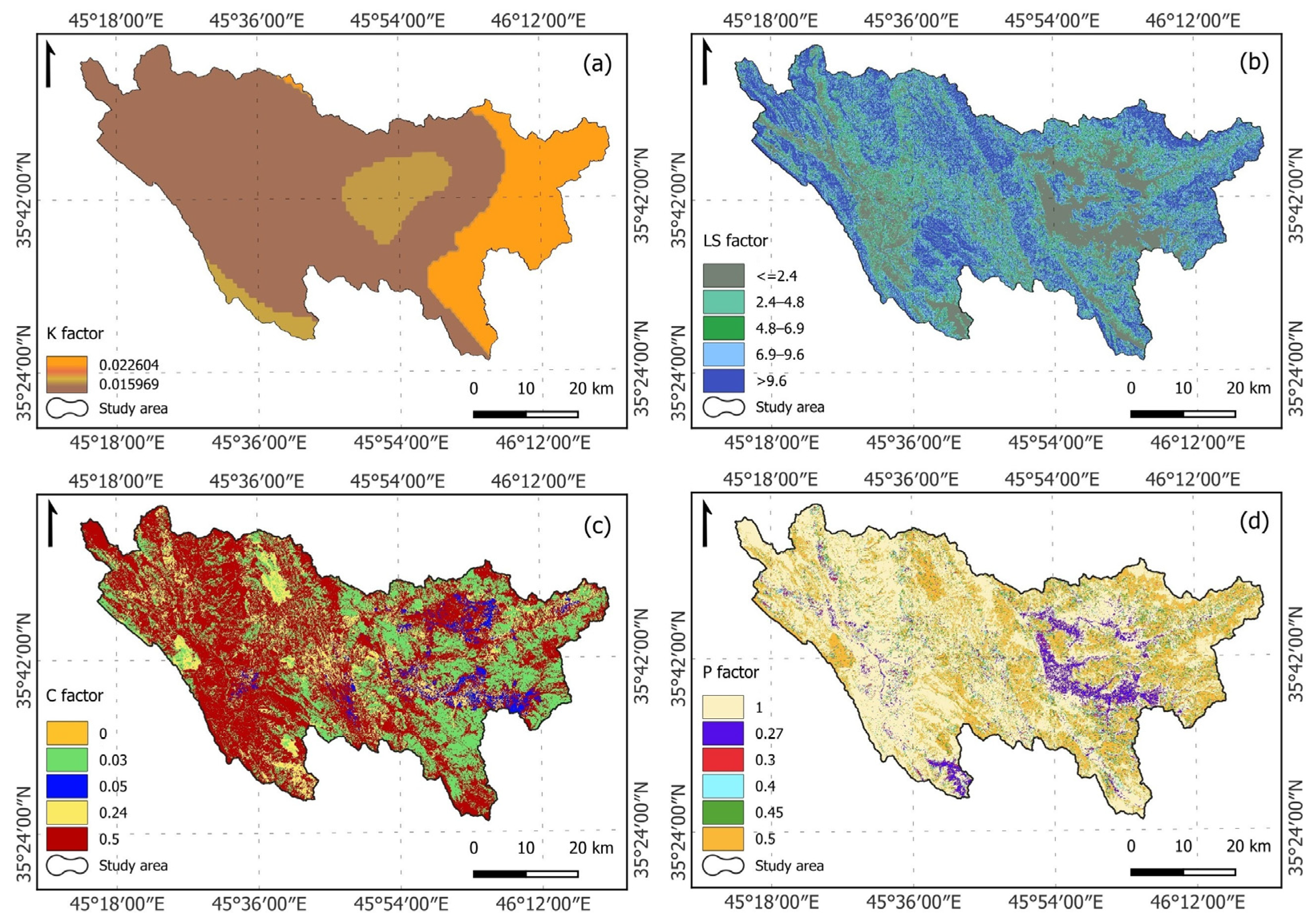
Three major soil units were identified in the Chami Qeshan Watershed, Lithic Leptosol, Akroskeletic Lithic Leptosol, and Vertisol, arranged in a descending spatial coverage order. According to the FAO HWSD dataset and the United States Department of Agriculture (USDA) textural triangle, loam soil texture dominates the majority of the studied region, followed by the sandy loam textural class, which covers the eastern geographical extent of CQW. The least prevailing soil textural category is clay, which visually appears as two patches in the middle and southeastern range of the area of interest. As displayed in Figure 5a, the K values range from a minimum of 0.015969 t·ha·hr·ha⁻¹·MJ⁻¹·mm⁻¹ to a maximum of 0.022604 t·ha·hr·ha⁻¹·MJ⁻¹·mm⁻¹.

Figure 5. Maps of four RUSLE factors: (a) soil erodibility [t·ha·hr·ha⁻¹·MJ⁻¹·mm⁻¹], (b) slope length–steepness, (c) land cover management, and (d) soil conservation practice. Factors (b–d) are dimensionless.

The slopes of CQW vary between 0 and 76 degrees, with elevations ranging from 632 to 2755 m above sea level. Based on the 30-m pixel resolution CDEM, the attained slope length–steepness values for the study region ranged between 0 and 24.3, with a mean value of 6.8 and a standard deviation of 4.4. The high LS values typically corresponded with elevated terrains, whereas low values were consistently associated with plains and floodplains. As shown in Figure 5b, the LS map was divided into five categories for the RUSLE calculation: 0–2.4 (21.3%), 2.4–4.8 (16.3%), 4.8–6.9 (13.3%), 6.9–9.6 (20.8%), and larger than 9.6 (28.3%).

To quantify the cover management factor, the Chami Qeshan Watershed was first categorized into five LULC classes using 2014 Landsat 8 OLI data, specifically agriculture, bare land, grassland, shrubland, and settlement. The C values of RUSLE ranged from 0 to 0.5 in the research region, as illustrated in Figure 5c. The highest C value of 0.5 was observed for most of the downstream/western portion of CQW, which represents bare land and is largely prone to erosion, accounting for 54.74% of the total area. The moderate value of C, 0.24, corresponds to farming territory, which is irregularly dispersed throughout CQW and constitutes 13.03%. The upstream/eastern zone of CQW is characterized by two low C values of 0.03 and 0.05, which are associated with shrubland (29.15%) and grassland (3.07%), respectively. The restricted settlement showed a minimum C value of 0, portraying only 0.01% of the investigated domain and symbolizing no soil erosion potential.

The conservation practice factor has been established for this research based on the literature [47,63,64], Table 4, and satellite observations, which revealed that strip-cropping is the primary approach for controlling soil erosion. The Shin classification [65], adopted herein, integrates slope angle (in percent) and applied farming techniques to compute the P factor for green areas. In this study, the p values ranged from 0.27 to 1 (Figure 5d), where low values indicate highly effective erosion-resistance management measures and high values imply no human-made erosion-resistance interventions. The maximum p value of 1 was reported for most of CQW, reflecting territories with no applied conservation practices, which make up 54.82% of the area. Likewise, the p values of 0.5 (25.37%), 0.45 (8%), 0.4 (4.48%), and 0.3 (2.54%) indicate heterogeneous soil conservation applications across the region of interest. The plains north of Penjwen town and northeast of Sulaymaniyah city (purple) show a minimum p value of 0.27 (4.79%), signifying zones where consistent erosion-prevention measures are practiced.

3.2. Estimation of Soil Loss and Sediment Yield

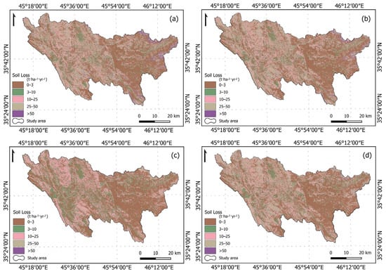
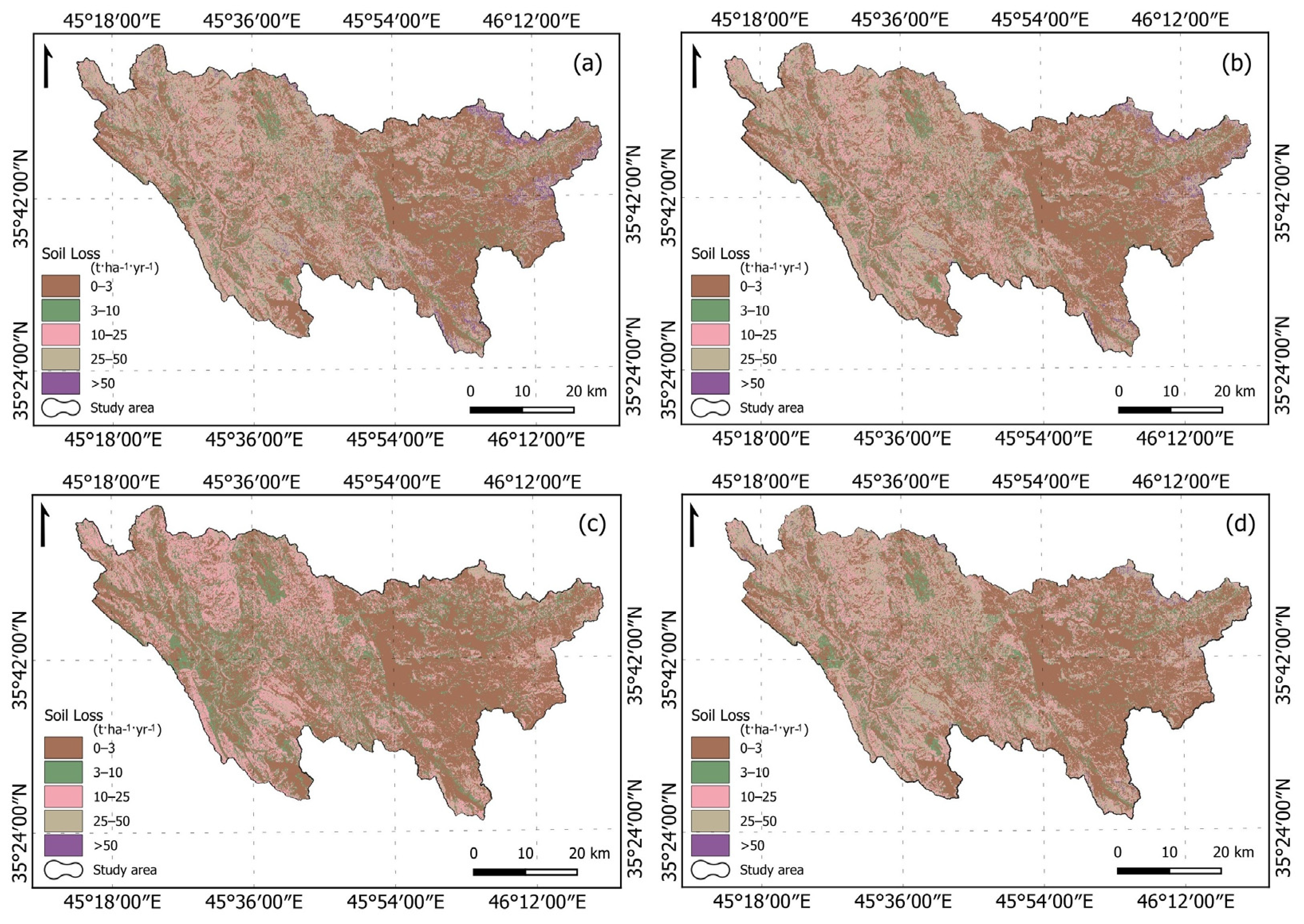
The soil loss rates in the Chami Qeshan Watershed were quantified by overlaying RUSLE input thematic layers in the QGIS environment at a 30-m × 30-m pixel resolution. Under the adopted RUSLE parameterization, the model estimated a mean soil loss based on OPD, CHIRPS, MERRA-2, and TRMM datasets of 13.26 t·ha⁻¹·yr⁻¹, 12.18 t·ha⁻¹·yr⁻¹, 7.40 t·ha⁻¹·yr⁻¹, and 11.05 t·ha⁻¹·yr⁻¹, respectively. To better understand the scope and severity of soil erosion in CQW, the obtained SL maps were categorized into five classes after Othman [35] as follows: very low (0–3), low (3–10), moderate (10–25), high (25–50), and very high (>50) (Figure 6). The very low class (43%) of the OPD-based SL (Figure 6a) is largely distributed in the eastern part of CQW, i.e., Penjwen plain and its neighboring areas, as well as the floodplains. The low class (15%) is irregularly dispersed across the investigated watershed. The moderate soil loss class (20%) occurs mostly in the western half of CQW, signifying, to a certain extent, terrains with limited greenery masses. At the same time, the high class (19%) is scattered concurrently with the intermediate class and dominates elevated landscapes. The least disseminated class is very high (3%), which is located mainly in the far northeast of CQW. As depicted in Figure 6b,d, a comparable spatial pattern for both the CHIRPS-based SL map (very low = 44%, low = 15%, moderate = 21%, high = 19%, and very high = 2%) and TRMM-based SL map (very low = 45%, low = 16%, moderate = 22%, high = 17%, and very high = 1%) was observed in the investigated basin. In contrast to earlier findings, the SL map created using the MERRA-2 product showed the highest proportion of the very low class (50%) (Figure 6c) and a close-to-zero fraction for the very high class. In addition, the low category (21%) was higher, whereas the moderate category (24%) was slightly more developed, and the high class (5%) in the soil loss map was considerably underestimated. It is pertinent to note that the latter SL thematic layer displayed a roughly corresponding spatial distribution of its classes to the previously mentioned RUSLE outcomes.

Figure 6. Spatial distribution maps of modeled soil loss estimates (RUSLE) in CQW resulted from four different precipitation-based R factors: (a) OPD, (b) CHIRPS, (c) MERRA-2, and (d) TRMM.

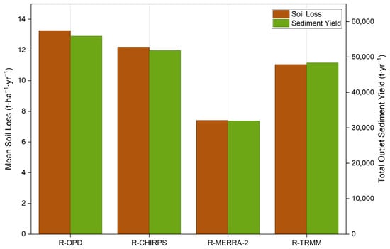
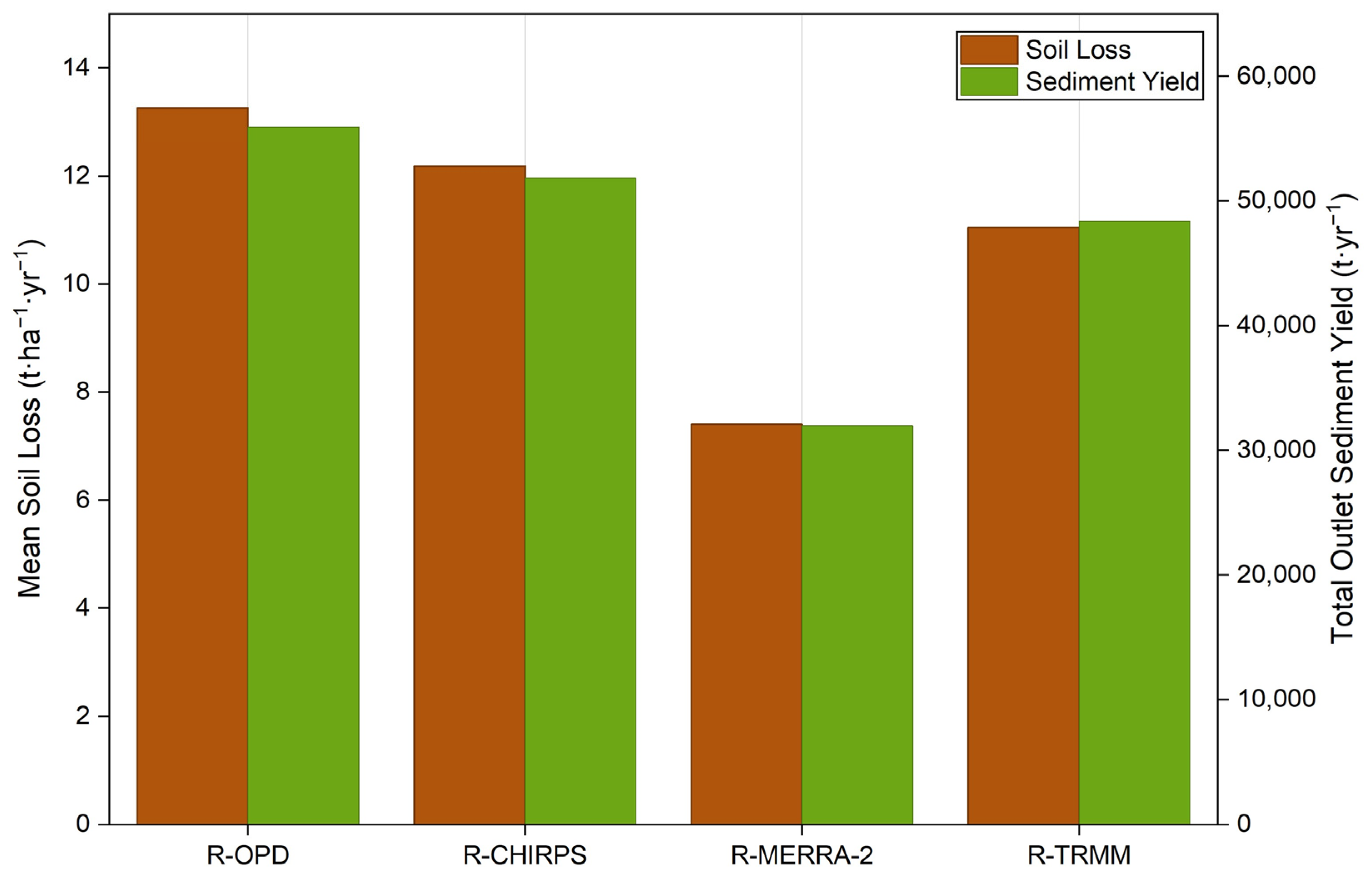
To estimate sediment yield from CQW, we first calculated the IC-based SDR using the arithmetic expression in Equations (12)–(15), yielding values ranging from 0 to 0.776, with a mean value of 0.012. It is important to clarify that the reported mean SDR of 0.012 represents the arithmetic spatial mean of the IC-based SDR raster and is not used directly in calculating total sediment yield. Thus, we computed the total outlet SY from the Chami Qeshan Watershed through pixel-wise integration of the RUSLE-derived soil erosion and IC-based SDR layers (Equation (16)) in the QGIS environment. This technique provides noteworthy insight into potential sediment delivery from the studied catchment. The RUSLE–SDR framework estimated total outlet sediment yield of 55,933 t·yr⁻¹, 51,826 t·yr⁻¹, 31,962 t·yr⁻¹, and 48,371 t·yr⁻¹ using the OPD, CHIRPS, MERRA-2, and TRMM products, respectively, under the adopted parameterization. Figure 7 provides a visual comparison between model-derived estimates of mean SL (ton per hectare per year) and total outlet SY (ton per year) for the Chami Qeshan Watershed, using different rainfall–runoff erosivity sources.

Figure 7. Double bar graph displays estimated mean soil loss and total outlet sediment yield for CQW based on four different R factors.

3.3. Statistical Analysis

This study evaluated the association between soil erosion outcomes and input variables using a correlational examination, as shown in Table 5. The Pearson correlation analysis exposed considerable differences among the spatial patterns of the four rainfall erosivity estimates. In other words, R1 and R2 exhibited a strong positive correlation (r = 0.92), whereas R3 exhibited negative correlations with R1 (r = −0.91) and R2 (r = −0.74). Moreover, the relatively strong correlation between C and P (r = 0.75) refers to significant spatial covariance between these two input variables. Although C and P were developed independently, this link may reflect the spatial correspondence between land-cover/management circumstances represented by C and the slope/assumed strip-cropping-practice classes used to assign P. The modeled soil-loss estimates (i.e., SL1–SL4) showed moderate positive associations with LS (r = 0.56–0.57), C (r = 0.50–0.61), and P (r = 0.48–0.63), whereas their associations with R and K were typically weaker. Nevertheless, these relationships should be interpreted with caution because all soil loss estimates share the identical K, LS, C, and P layers and vary mainly in their R input. Therefore, the correlations between the RUSLE factors and resulting soil loss estimates represent model-dependent statistical associations and should not be interpreted as independent evidence of model robustness or causal process control.

Table 5. Pearson correlation matrix of the implemented variables and resultant soil loss estimates.

	R1	R2	R3	R4	K	LS	C	P	SL1	SL2	SL3	SL4
R1	1.00	0.92	−0.91	−0.35	0.33	−0.17	−0.21	−0.21	−0.15	−0.19	−0.22	−0.23
R2	0.92	1.00	−0.74	−0.17	0.17	−0.21	−0.16	−0.17	−0.17	−0.20	−0.24	−0.24
R3	−0.91	−0.74	1.00	0.50	−0.49	0.13	0.22	0.20	0.13	0.17	0.19	0.21
R4	−0.35	−0.17	0.50	1.00	−0.74	0.04	0.19	0.16	0.07	0.09	0.10	0.14
K	0.33	0.17	−0.49	−0.74	1.00	0.03	−0.18	−0.14	0.00	−0.02	−0.03	−0.06
LS	−0.17	−0.21	0.13	0.04	0.03	1.00	−0.04	0.08	0.56	0.57	0.57	0.57
C	−0.21	−0.16	0.22	0.19	−0.18	−0.04	1.00	0.75	0.61	0.61	0.53	0.50
P	−0.21	−0.17	0.20	0.16	−0.14	0.08	0.75	1.00	0.62	0.63	0.48	0.50
SL1	−0.15	−0.17	0.13	0.07	0.00	0.56	0.61	0.62	1.00	1.00	0.83	0.81
SL2	−0.19	−0.20	0.17	0.09	−0.02	0.57	0.61	0.63	1.00	1.00	0.83	0.82
SL3	−0.22	−0.24	0.19	0.10	−0.03	0.57	0.53	0.48	0.83	0.83	1.00	0.88
SL4	−0.23	−0.24	0.21	0.14	−0.06	0.57	0.50	0.50	0.81	0.82	0.88	1.00

The values 1, 2, 3, and 4 denote OPD-, CHIRPS-, MERRA-2-, and TRMM-based values, respectively.

4. Discussion

As stated in the literature review section, few prior studies have examined and assessed soil erosion and its adverse implications in the Zagros Mountains region. However, little was found on the association between different types of satellite-derived precipitation products and their application to the RUSLE-SDR model. Consequently, the purpose of this work was to evaluate the efficiency of three precipitation estimates (i.e., CHIRPS, MERRA-2, and TRMM) in conjunction with observed precipitation measurements for predicting soil loss and sediment yield in the Chami Qeshan Watershed. Figure 3 displays linear regression between observed annual precipitation and CHIRPS, MERRA-2, and TRMM datasets. CHIRPS showed the strongest positive linear relationship with observed precipitation (R² = 0.633) and the lowest error (RMSE = 177.8 mm/year), followed by TRMM (R² = 0.478 and RMSE = 240 mm/year) and lastly MERRA-2 (R² = 0.353 and RMSE = 452.1 mm/year). In summary, the combined assessment of R² and RMSE identifies CHIRPS as the best-performing product for reproducing measured annual precipitation inconsistency, followed by TRMM and then MERRA-2 within the circumstances of the present study.

The rainfall–runoff erosivity factor derived from the datasets follows a pattern consistent with precipitation magnitude. As shown in Figure 4, CHIRPS yielded the highest rainfall–runoff erosivity range of 312.9–394.2 MJ·mm·ha⁻¹·hr⁻¹·yr⁻¹, followed by TRMM (R = 284.6–336.5 MJ·mm·ha⁻¹·hr⁻¹·yr⁻¹) and MERRA-2 (R = 208.8–215.1 MJ·mm·ha⁻¹·hr⁻¹·yr⁻¹). As a result, CHIRPS seems appropriate for regional soil erosion and land degradation studies. In contrast, without additional bias correction, MERRA-2 is inadequate for rainfall-erosivity calculations in the research domain. The substantial association between precipitation magnitude and rainfall–runoff erosivity throughout all products confirms the importance of accurately estimating rainfall variability before further evaluations. Overall, CHIRPS provides the closest approximation of observed precipitation and rainfall–runoff erosivity, TRMM shows intermediate performance, whereas MERRA-2 considerably underestimates both magnitude and variability. The estimation error could be attributed to satellite retrieval limitations across complicated terrain with diverse precipitation regimes, such as the Zagros Mountain Range, or to other variables. Thus, future research should consider sensitivity analyses using native resolutions, a common coarser grid, and alternative interpolation methods to evaluate the reliability of the findings. The comparison of the precipitation products is therefore interpreted primarily in terms of their precipitation-estimation performance and watershed-scale R, SL, and SY patterns, rather than assuming that all products provide equivalent 30 m spatial information.

As demonstrated in Figure 3 and Figure 7, the model-based soil loss and sediment yield estimates exhibited an overall trend that is in agreement with the employed precipitation extents. In other words, under the implemented RUSLE parameterization, the model estimated mean soil loss of 13.26 t·ha⁻¹·yr⁻¹, 12.18 t·ha⁻¹·yr⁻¹, 7.40 t·ha⁻¹·yr⁻¹, and 11.05 t·ha⁻¹·yr⁻¹ using OPD, CHIRPS, MERRA-2, and TRMM datasets, respectively. Our method is consistent with earlier investigations carried out in data-scarce Iranian mountainous basins. For instance, the research of [78] applied RUSLE–GIS in the Gharesoo River Basin in northern Iran to estimate potential soil erosion and assess alternative land-use planning scenarios. Their study reported average potential soil erosion rates ranging from 13.86 t·ha⁻¹·yr⁻¹ to 18.65 t·ha⁻¹·yr⁻¹ under different land-use conditions. Likewise, another study by [79] explicitly implemented a scenario-based RUSLE–SEDD framework in northeastern Iran to investigate erosion and sedimentation and the soil-conservation function of rangeland vegetation. They estimated mean annual soil erosion of 13.46 t·ha⁻¹·yr⁻¹ in the investigated region. These studies demonstrate the applicability of RUSLE-based methods for spatial and scenario-based assessment in data-scarce mountainous regions. However, these published values are used only to provide contextual evidence that the magnitude of the modeled erosion rates in the current study is within the range reported for neighboring basins.

As an exploratory evaluation, the Pearson correlation analysis exposed noteworthy differences in the spatial patterns of rainfall erosivity estimates. R1 and R2 were strongly and positively correlated (r = 0.92), whereas R3 was negatively correlated with R1 (r = −0.91) and R2 (r = −0.74). The strong C–P correlation (r = 0.75) indicates spatial covariance, potentially reflecting correspondence between land-cover patterns and slope/bare land/assumed strip-cropping classes used to assign C and P, respectively. At the same time, estimated soil loss exhibited moderate associations with LS (r = 0.56–0.57), C (r = 0.50–0.61), and P (r = 0.48–0.63), but weaker associations with R and K. Nonetheless, because these factors are inputs to RUSLE and the soil-loss scenarios share identical K, LS, C, and P layers, these correlations characterize model-dependent associations rather than independent evidence of causal process control or model robustness.

The outcomes of the present investigation should be considered with caution, as there are limitations that need to be addressed in subsequent studies. As the empirical R-factor formulation may represent a critical source of uncertainty in absolute SL and SY estimates, subsequent research should evaluate and compare multiple regionally applicable R equations based on high-temporal-resolution rainfall observations and test their performance locally to identify the most suitable formulation for the investigated watershed. Another crucial constraint of this work was the absence of periodic sediment yield records to validate the results, which is attributed to the absence of permanent gauge stations in the transboundary CQW [40]. Therefore, future validation and uncertainty analysis should prioritize acquiring reservoir bathymetric surveys, suspended-sediment measurements, historical reservoir-capacity changes, and/or field-based erosion observations. An additional drawback is the inability of RUSLE to account for complicated geomorphic processes such as gully erosion, riverbank erosion, and mass wasting, which occur frequently in areas that experience heavy rainfall and human-induced disturbance, such as deforestation and mining [5,64].

There are additional uncertainties stemming from the computation of C and P inputs of RUSLE, as they are derived from the published literature and have not been amended to the considered catchment. Future studies are needed to integrate higher-resolution inputs (e.g., time-series land use data, drone surveys, detailed pedological maps, and LiDAR-derived DEMs) and implement process-based models (e.g., WEPP, SWAT, and EUROSEM) to better represent hydrological processes and extreme climate incidents. An inevitable progression of this work is to implement global sensitivity/variance-decomposition approaches combined with spatially explicit analyses to deliver a firmer separation of model-structural effects from process controls. Once adequate sediment yield observations become available, subsequent studies should incorporate spatial validation, hotspot/exceedance analysis, and uncertainty estimates accounting for spatial autocorrelation to provide a more rigorous evaluation of model sensitivity and spatial robustness. Further research should combine RUSLE with machine learning techniques, such as artificial neural networks [80] and random forests [81], which could provide an effective means of improving outcome accuracy. Alongside this, it can be worthwhile to establish awareness campaigns to inform the local community about soil erosion and its adverse repercussions.

5. Conclusions

The variation between observed precipitation measurements and the satellite-derived precipitation estimates, as well as their implications for quantifying soil loss and sediment yield, validate the hypotheses of this research. This study sought to determine which precipitation product (i.e., CHIRPS, MERRA-2, and TRMM) is particularly effective at estimating soil loss and sediment yield in the transboundary CQW using the combined RUSLE-SDR model. This investigation has found that CHIRPS provides the best reproduction of annual precipitation and the closest agreement with gauge-driven reference simulations of SL and SY. The eastern part of CQW, precisely the Penjwen agricultural plain, experienced low soil loss rates due to its abundant vegetation cover, implemented conservation practices, and gentle slope. The correlation analysis disclosed significant differences among the spatial patterns of rainfall erosivity products, while modeled soil loss was moderately associated with LS, C, and P. As these variables are inputs to RUSLE and the soil-loss scenarios utilize the same K, LS, C, and P layers, these relationships should be regarded as model-dependent associations rather than valid proof of independent process control or model robustness. Taken together, it is crucial to highlight that the results of the technique outlined herein can be continually enhanced as the accuracy and reliability of the input data increase. Despite the shortage of in situ data, this research provides insights into integrating satellite-derived products, RUSLE, IC-based SDR, and QGIS to predict soil loss and sediment yield in mountainous catchments. This study could assist researchers and policymakers in finding reasonable meteorological data for mapping soil vulnerability in remote basins.

Beyond its current implications for soil conservation, this work establishes a procedural foundation for future research into the potential consequences of climate change on soil erosion and sediment yield in the investigated region. Changes in precipitation patterns and rainfall erosivity could affect the quantity and spatial distribution of soil loss and sediment delivery, especially in mountainous zones featuring steep slopes and erratic rainfall. Nevertheless, this study was not designed to directly evaluate long-term climate trends or future climate scenarios; therefore, the determined erosion patterns should not be perceived as an explicit indicator of climate change effects. Further studies could expand the present RUSLE–SDR framework by leveraging long-term precipitation data and climate projections to assess potential changes in erosion risk and sediment delivery under various climate scenarios. In addition, terrestrial and aquatic ecosystems may be affected by the identified erosion-prone spots. Soil degradation and sediment deposition can affect soil quality, habitat conditions, and aquatic ecosystem functioning, thereby affecting local biodiversity. However, these ecological implications were not directly assessed in this work and require additional examination by combining sediment assessments with ecological and biodiversity measures. Adopting such an integrated scheme would foster more comprehensive soil conservation and watershed management strategies in response to changing environmental conditions.

References

- Apollo, M.; Andreychouk, V.; Bhattarai, S. Short-Term Impacts of Livestock Grazing on Vegetation and Track Formation in a High Mountain Environment: A Case Study from the Himalayan Miyar Valley (India). Sustainability 2018, 10, 951. [Google Scholar] [CrossRef] [Scilit]
- Thomas, J.; Joseph, S.; Thrivikramji, K.P. Estimation of Soil Erosion in a Rain Shadow River Basin in the Southern Western Ghats, India Using RUSLE and Transport Limited Sediment Delivery Function. Int. Soil Water Conserv. Res. 2018, 6, 111–122. [Google Scholar] [CrossRef] [Scilit]
- Sharda, V.N.; Ojasvi, P.R. A Revised Soil Erosion Budget for India: Role of Reservoir Sedimentation and Land-use Protection Measures. Earth Surf. Process. Landf. 2016, 41, 2007–2023. [Google Scholar] [CrossRef] [Scilit]
- Patil, M.; Patel, R.; Saha, A. Sediment Yield and Soil Loss Estimation Using GIS Based Soil Erosion Model: A Case Study in the MAN Catchment, Madhya Pradesh, India. Environ. Sci. Proc. 2021, 8, 26. [Google Scholar] [CrossRef] [Scilit]
- Ghimire, S.; Singh, U.; Panthi, K.K.; Bhattarai, P.K. Spatial Sediment Erosion and Yield Using RUSLE Coupled with Distributed SDR Model. Water 2024, 16, 3549. [Google Scholar] [CrossRef] [Scilit]
- Laflen, J.M.; Elliot, W.J.; Flanagan, D.C.; Meyer, C.R.; Nearing, M.A. WEPP-Predicting Water Erosion Using a Process-Based Model. J. Soil Water Conserv. 1997, 52, 96–102. [Google Scholar] [CrossRef] [Scilit]
- Al-Mukhtar, M.; Dunger, V.; Merkel, B. Runoff and Sediment Yield Modeling by Means of WEPP in the Bautzen Dam Catchment, Germany. Environ. Earth Sci. 2014, 72, 2051–2063. [Google Scholar] [CrossRef] [Scilit]
- Flanagan, D.C.; Frankenberger, J.R.; Renschler, C.S.; Coreil, C.B.; David, O.; Srivastava, A.; Jame, S.A.; McGehee, R.P. Water Erosion Prediction Project (WEPP) Model 2024 Status. In Proceedings of the 2024 Anaheim, Anaheim, CA, USA, 28–31 July 2024; American Society of Agricultural and Biological Engineers: St. Joseph, MI, USA, 2024. [Google Scholar]
- Morgan, R.P.C.; Quinton, J.N.; Smith, R.E.; Govers, G.; Poesen, J.W.A.; Auerswald, K.; Chisci, G.; Torri, D.; Styczen, M.E. The European Soil Erosion Model (EUROSEM): A Dynamic Approach for Predicting Sediment Transport from Fields and Small Catchments. Earth Surf. Process. Landf. 1998, 23, 527–544. [Google Scholar] [CrossRef] [Scilit]
- Arnold, J.G.; Srinivasan, R.; Muttiah, R.S.; Williams, J.R. LARGE AREA HYDROLOGIC MODELING AND ASSESSMENT PART I: MODEL DEVELOPMENT1. J. Am. Water Resour. Assoc. 1998, 34, 73–89. [Google Scholar] [CrossRef] [Scilit]
- Ferro, V.; Porto, P. Sediment Delivery Distributed (SEDD) Model. J. Hydrol. Eng. 2000, 5, 411–422. [Google Scholar] [CrossRef] [Scilit]
- Wischmeier, W.H.; Smith, D.D. Predicting Rainfall Erosion Losses: A Guide to Conservation Planning; Agriculture Handbook Number 537; United States Department of Agriculture: Washington, DC, USA, 1978.
- Renard, K.G.; Foster, G.R.; Weesies, G.A.; McCool, D.K.; Yoder, D.C. Predicting Soil Erosion by Water: A Guide to Conservation Planning with the Revised Universal Soil Loss Equation (RUSLE); Agriculture Handbook Number 703; United States Department of Agriculture: Washington, DC, USA, 1997; p. 407.
- Benavidez, R.; Jackson, B.; Maxwell, D.; Norton, K. A Review of the (Revised) Universal Soil Loss Equation ((R)USLE): With a View to Increasing Its Global Applicability and Improving Soil Loss Estimates. Hydrol. Earth Syst. Sci. 2018, 22, 6059–6086. [Google Scholar] [CrossRef] [Scilit]
- Terefe, B.; Melese, T.; Tsegaye, A.; Afework, A.; Yibeltal, T.; Anagaw, A.; Temesgen, F.; Belay, T.; Assefa, G.; Mencho, B.B. Soil Loss Estimation in Ethiopia: A Comprehensive Review of the RUSLE Model Integrated with Geospatial Technologies. Discov. Sustain. 2025, 6, 334. [Google Scholar] [CrossRef] [Scilit]
- Renard, K.G.; Foster, G.R.; Weesies, G.A.; Porter, J.P. RUSLE: Revised Universal Soil Loss Equation. J. Soil Water Conserv. 1991, 46, 30–33. [Google Scholar] [CrossRef] [Scilit]
- Al-Kakey, O.; Al-Mukhtar, M.; Berhanu, S.; Dunger, V. Assessing CFSR Climate Data for Rainfall-Runoff Modeling over an Ungauged Basin between Iraq and Iran. Kuwait J. Sci. 2023, 50, 405–414. [Google Scholar] [CrossRef] [Scilit]
- Funk, C.; Peterson, P.; Landsfeld, M.; Pedreros, D.; Verdin, J.; Shukla, S.; Husak, G.; Rowland, J.; Harrison, L.; Hoell, A.; et al. The Climate Hazards Infrared Precipitation with Stations—A New Environmental Record for Monitoring Extremes. Sci. Data 2015, 2, 150066. [Google Scholar] [CrossRef] [Scilit] [PubMed]
- Gelaro, R.; McCarty, W.; Suárez, M.J.; Todling, R.; Molod, A.; Takacs, L.; Randles, C.A.; Darmenov, A.; Bosilovich, M.G.; Reichle, R.; et al. The Modern-Era Retrospective Analysis for Research and Applications, Version 2 (MERRA-2). J. Clim. 2017, 30, 5419–5454. [Google Scholar] [CrossRef] [Scilit] [PubMed]
- Kummerow, C.; Barnes, W.; Kozu, T.; Shiue, J.; Simpson, J. The Tropical Rainfall Measuring Mission (TRMM) Sensor Package. J. Atmos. Ocean. Technol. 1998, 15, 809–817. [Google Scholar] [CrossRef] [Scilit]
- Hamal, K.; Sharma, S.; Khadka, N.; Baniya, B.; Ali, M.; Shrestha, M.S.; Xu, T.; Shrestha, D.; Dawadi, B. Evaluation of MERRA-2 Precipitation Products Using Gauge Observation in Nepal. Hydrology 2020, 7, 40. [Google Scholar] [CrossRef] [Scilit]
- Goodarzi, M.R.; Pooladi, R.; Niazkar, M. Evaluation of Satellite-Based and Reanalysis Precipitation Datasets with Gauge-Observed Data over Haraz-Gharehsoo Basin, Iran. Sustainability 2022, 14, 13051. [Google Scholar] [CrossRef] [Scilit]
- Huang, N.; Fu, S.; Chen, B.; Huang, L.; Jin, W. Assessing the Performance of Water Vapor Products from ERA5 and MERRA-2 during Heavy Rainfall in the Guangxi Region of China. Atmosphere 2024, 15, 306. [Google Scholar] [CrossRef] [Scilit]
- Apaza-Vilca, C.; Mamani-Yupanqui, M.L.; Lujano, E. Performance Evaluation of the ERA5, MERRA-2, and PERSIANN-CDR Gridded Products in the Tambo Basin. Environ. Earth Sci. Proc. 2025, 32, 17. [Google Scholar] [CrossRef] [Scilit]
- Pellicone, G.; Caloiero, T.; Coscarelli, R.; Chiaravalloti, F. Assessment of Multiple Satellite Precipitation Products over Italy. Remote Sens. 2025, 17, 3772. [Google Scholar] [CrossRef] [Scilit]
- Delgado, D.; Sadaoui, M.; Ludwig, W.; Méndez, W. Spatio-Temporal Assessment of Rainfall Erosivity in Ecuador Based on RUSLE Using Satellite-Based High Frequency GPM-IMERG Precipitation Data. CATENA 2022, 219, 106597. [Google Scholar] [CrossRef] [Scilit]
- Li, X.; Ye, X.; Xu, C. Assessment of Satellite-Based Precipitation Products for Estimating and Mapping Rainfall Erosivity in a Subtropical Basin, China. Remote Sens. 2022, 14, 4292. [Google Scholar] [CrossRef] [Scilit]
- Subbarayan, S.; Sankriti, R. Mapping of Spatially Distributed Soil Erosion over the Tungabhadra River Sub-Basin (TRB) Using Satellite-Based Precipitation Products (SPPs) and RUSLE Modelling. Hydrology 2026, 13, 148. [Google Scholar] [CrossRef] [Scilit]
- Abebe, N.; Eekhout, J.; Vermeulen, B.; Boix-Fayos, C.; De Vente, J.; Grum, B.; Hoitink, T.; Baartman, J. The Potential and Challenges of the ‘RUSLE-IC-SDR’ Approach to Identify Sediment Dynamics in a Mediterranean Catchment. CATENA 2023, 233, 107480. [Google Scholar] [CrossRef] [Scilit]
- Guo, Z.; Wu, L.; Liu, S.; Zhang, H.; Du, B.; Ruan, B. An Integrated Watershed Modelling Framework to Explore the Covariation between Sediment Connectivity and Soil Erosion. Eur. J. Soil Sci. 2023, 74, e13412. [Google Scholar] [CrossRef] [Scilit]
- Yang, X.; Young, J.; Shi, H.; Zhu, Q.; Pulsford, I.; Chapman, G.; Moore, L.; Gormley, A.G.; Thackway, R.; Shepherd, T. Estimating Sediment Delivery Ratio Using the RUSLE-IC-SDR Approach at a Complex Landscape: A Case Study at the Lower Snowy River Area, Australia. J. Hydrol. 2024, 645, 132237. [Google Scholar] [CrossRef] [Scilit]
- Allafta, H.; Opp, C. Soil Erosion Assessment Using the RUSLE Model, Remote Sensing, and GIS in the Shatt Al-Arab Basin (Iraq-Iran). Appl. Sci. 2022, 12, 7776. [Google Scholar] [CrossRef] [Scilit]
- Ahmadi Mirghaed, F.; Souri, B.; Mohammadzadeh, M.; Salmanmahiny, A.; Mirkarimi, S.H. Evaluation of the Relationship between Soil Erosion and Landscape Metrics across Gorgan Watershed in Northern Iran. Environ. Monit. Assess. 2018, 190, 643. [Google Scholar] [CrossRef] [Scilit] [PubMed]
- Ustaoğlu, B.; İkiel, C.; Atalay Dutucu, A.; Koç, D.E. Erosion Susceptibility Analysis in Datça and Bozburun Peninsulas, Turkey. Iran. J. Sci. Technol. Trans. Sci. 2021, 45, 557–570. [Google Scholar] [CrossRef] [Scilit]
- Othman, A.; Obaid, A.; Al-Manmi, D.; Al-Maamar, A.; Hasan, S.; Liesenberg, V.; Shihab, A.; Al-Saady, Y. New Insight on Soil Loss Estimation in the Northwestern Region of the Zagros Fold and Thrust Belt. IJGI 2021, 10, 59. [Google Scholar] [CrossRef] [Scilit]
- Othman, A.A.; Ali, S.S.; Salar, S.G.; Obaid, A.K.; Al-Kakey, O.; Liesenberg, V. Insights for Estimating and Predicting Reservoir Sedimentation Using the RUSLE-SDR Approach: A Case of Darbandikhan Lake Basin, Iraq–Iran. Remote Sens. 2023, 15, 697. [Google Scholar] [CrossRef] [Scilit]
- Othman, A.A.; Ali, S.S.; Scheytt, T. Comparison between Multi RUSLE-SDR Models for Estimation of Reservoir Sedimentation: A Case Study of Dokan Lake Basin, Iraq–Iran. Environ. Earth Sci. 2024, 83, 419. [Google Scholar] [CrossRef] [Scilit]
- Mohammed, F.O.; Mohamed, A.I.; Gart, I.H.; Amin, D.A. Establishing of Soil Loss Tolerance Limit and Sediment Yield in Zagros Fold Thrust Belt: A Case Study in the Kanarwe River Basin, Iraq-Iran. Bull. Min. Res. Exp. 2025, 176, 76–92. [Google Scholar] [CrossRef] [Scilit]
- Al-Saady, Y.I.; Al-Suhail, Q.A.; Al-Tawash, B.S.; Othman, A.A. Drainage Network Extraction and Morphometric Analysis Using Remote Sensing and GIS Mapping Techniques (Lesser Zab River Basin, Iraq and Iran). Environ. Earth Sci. 2016, 75, 1243. [Google Scholar] [CrossRef] [Scilit]
- Al-Kakey, O.; Othman, A.A.; Al-Mukhtar, M.; Dunger, V. Proposing Optimal Locations for Runoff Harvesting and Water Management Structures in the Hami Qeshan Watershed, Iraq. IJGI 2023, 12, 312. [Google Scholar] [CrossRef] [Scilit]
- Othman, A.; Gloaguen, R. Improving Lithological Mapping by SVM Classification of Spectral and Morphological Features: The Discovery of a New Chromite Body in the Mawat Ophiolite Complex (Kurdistan, NE Iraq). Remote Sens. 2014, 6, 6867–6896. [Google Scholar] [CrossRef] [Scilit]
- Funk, C.C.; Peterson, P.J.; Landsfeld, M.F.; Pedreros, D.H.; Verdin, J.P.; Rowland, J.D.; Romero, B.E.; Husak, G.J.; Michaelsen, J.C.; Verdin, A.P. A Quasi-Global Precipitation Time Series for Drought Monitoring; U.S. Geological Survey Data Series 832; USGS: Reston, VA, USA, 2014; p. 4. [Google Scholar] [CrossRef] [Scilit]
- OpenTopography; European Space Agency. Airbus Copernicus DEM. Available online: https://portal.opentopography.org/raster?opentopoID=OTSDEM.032021.4326.3 (accessed on 22 July 2022).
- Nachtergaele, F.; van Velthuizen, H.; van Engelen, V.; Fischer, G.; Jones, A.; Montanarella, L.; Petri, M.; Prieler, S.; Teixeira, E.; Shi, X. Harmonized World Soil Database, Version 1.2; FAO: Rome, Italy; IIASA: Laxenburg, Austria, 2012; pp. 1–50.
- Al-Saady, Y.; Merkel, B.; Al-Tawash, B.; Al-Suhail, Q. Land Use and Land Cover (LULC) Mapping and Change Detection in the Little Zab River Basin (LZRB), Kurdistan Region, NE Iraq and NW Iran. Freib. Online Geosci. 2015, 43, 1–32. [Google Scholar]
- Alewell, C.; Borrelli, P.; Meusburger, K.; Panagos, P. Using the USLE: Chances, Challenges and Limitations of Soil Erosion Modelling. Int. Soil Water Conserv. Res. 2019, 7, 203–225. [Google Scholar] [CrossRef] [Scilit]
- Menghis, T.B.; Zdruli, P.; Dobos, E. A GIS-Based Approach to Soil Erosion Risk Assessment Using RUSLE: The Case of the Mai Nefhi Watershed, Barka River Basin, Eritrea. Earth 2025, 6, 58. [Google Scholar] [CrossRef] [Scilit]
- Birhanu, L.; Mekonen, Y.; Tilahun, A.; Amsalu, N.; Balzter, H. Impact of Land Use and Land Cover Change on Soil Erosion in Dondor Watershed, Blue Nile Basin, Northwestern Ethiopia. Sustainability 2024, 16, 10421. [Google Scholar] [CrossRef] [Scilit]
- Bodenstein, D.; Clarke, C.; Watson, A.; Miller, J.; Van Der Westhuizen, S.; Rozanov, A. Evaluation of Global and Continental Scale Soil Maps for Southern Africa Using Selected Soil Properties. CATENA 2022, 216, 106381. [Google Scholar] [CrossRef] [Scilit]
- Mohammed Hameed, H. Soil Erosion Assessment within the Erbil Watershed Using Geo-Informatics Technology. HUJ 2021, 6, 311–329. [Google Scholar] [CrossRef] [Scilit]
- Doulabian, S.; Shadmehri Toosi, A.; Humberto Calbimonte, G.; Ghasemi Tousi, E.; Alaghmand, S. Projected Climate Change Impacts on Soil Erosion over Iran. J. Hydrol. 2021, 598, 126432. [Google Scholar] [CrossRef] [Scilit]
- Mouris, K.; Schwindt, S.; Haun, S.; Morales Oreamuno, M.F.; Wieprecht, S. Introducing Seasonal Snow Memory into the RUSLE. J. Soils Sediments 2022, 22, 1609–1628. [Google Scholar] [CrossRef] [Scilit]
- Sharpley, A.N.; Williams, J.R. EPIC. Erosion/Productivity Impact Calculator: 1. Model Documentation. 2. User Manual; USDA: Washington, DC, USA, 1990.
- Phinzi, K.; Ngetar, N.S. The Assessment of Water-Borne Erosion at Catchment Level Using GIS-Based RUSLE and Remote Sensing: A Review. Int. Soil Water Conserv. Res. 2019, 7, 27–46. [Google Scholar] [CrossRef] [Scilit]
- Kerven, G.L.; Menzies, N.W.; Geyer, M.D. Analytical Methods and Quality Assurance: Soil Carbon Determination by High Temperature Combustion—A Comparison with Dichromate Oxidation Procedures and the Influence of Charcoal and Carbonate Carbon on the Measured Value. Communic. Soil Sci. Plant Anal. 2000, 31, 1935–1939. [Google Scholar] [CrossRef] [Scilit]
- Panagos, P.; Meusburger, K.; Ballabio, C.; Borrelli, P.; Alewell, C. Soil Erodibility in Europe: A High-Resolution Dataset Based on LUCAS. Sci. Total Environ. 2014, 479–480, 189–200. [Google Scholar] [CrossRef] [Scilit] [PubMed]
- Chadli, K. Estimation of Soil Loss Using RUSLE Model for Sebou Watershed (Morocco). Model. Earth Syst. Environ. 2016, 2, 51. [Google Scholar] [CrossRef] [Scilit]
- Biru, M.K.; Gadisa, C.W.; Dirbaba, N.B.; Nunes, M.R. Land Use Changes and Their Impacts on Soil Erosion in a Fragile Ecosystem of the Ethiopian Highlands. Land 2025, 14, 1473. [Google Scholar] [CrossRef] [Scilit]
- Zerihun, M.; Mohammedyasin, M.S.; Sewnet, D.; Adem, A.A.; Lakew, M. Assessment of Soil Erosion Using RUSLE, GIS and Remote Sensing in NW Ethiopia. Geoderma Reg. 2018, 12, 83–90. [Google Scholar] [CrossRef] [Scilit]
- Moore, I.D.; Burch, G.J. Physical Basis of the Length-slope Factor in the Universal Soil Loss Equation. Soil Sci. Soc. Amer. J. 1986, 50, 1294–1298. [Google Scholar] [CrossRef] [Scilit]
- Li, Y.; Qi, S.; Liang, B.; Ma, J.; Cheng, B.; Ma, C.; Qiu, Y.; Chen, Q. Dangerous Degree Forecast of Soil Loss on Highway Slopes in Mountainous Areas of the Yunnan–Guizhou Plateau (China) Using the Revised Universal Soil Loss Equation. Nat. Hazards Earth Syst. Sci. 2019, 19, 757–774. [Google Scholar] [CrossRef] [Scilit]
- Gupta, S.; Ojha, C.S.P.; Singh, V.P.; Adeloye, A.J.; Jain, S.K. Pixel-Based Soil Loss Estimation and Prioritization of North-Western Himalayan Catchment Based on Revised Universal Soil Loss Equation (RUSLE). Sustainability 2023, 15, 15177. [Google Scholar] [CrossRef] [Scilit]
- Karamage, F.; Zhang, C.; Liu, T.; Maganda, A.; Isabwe, A. Soil Erosion Risk Assessment in Uganda. Forests 2017, 8, 52. [Google Scholar] [CrossRef] [Scilit]
- Santos, A.D.S.; Silva Júnior, J.F.D.; Santos, L.D.S.; Alencar Sobrinho, R.J.; Amorim, E.C.; Fernandes, G.S.T.; Silva, E.F.D.; Silva, T.G.F.D.; De Lima, J.L.M.P.; Jardim, A.M.D.R.F. Identification of Priority Areas for the Control of Soil Erosion and the Influence of Terrain Factors Using RUSLE and GIS in the Caeté River Basin, Brazilian Amazon. Earth 2025, 6, 35. [Google Scholar] [CrossRef] [Scilit]
- Shin, G.J. The Analysis of Soil Erosion Analysis in Watershed Using GIS. Ph.D. Dissertation, Department of Civil Engineering, Gang-Won National University, Chuncheon, Republic of Korea, 1999. [Google Scholar]
- Azizian, A.; Koohi, S. The Effects of Applying Different DEM Resolutions, DEM Sources and Flow Tracing Algorithms on LS Factor and Sediment Yield Estimation Using USLE in Barajin River Basin (BRB), Iran. Paddy Water Environ. 2021, 19, 453–468. [Google Scholar] [CrossRef] [Scilit]
- Borselli, L.; Cassi, P.; Torri, D. Prolegomena to Sediment and Flow Connectivity in the Landscape: A GIS and Field Numerical Assessment. CATENA 2008, 75, 268–277. [Google Scholar] [CrossRef] [Scilit]
- Cavalli, M.; Trevisani, S.; Comiti, F.; Marchi, L. Geomorphometric Assessment of Spatial Sediment Connectivity in Small Alpine Catchments. Geomorphology 2013, 188, 31–41. [Google Scholar] [CrossRef] [Scilit]
- Vigiak, O.; Borselli, L.; Newham, L.T.H.; McInnes, J.; Roberts, A.M. Comparison of Conceptual Landscape Metrics to Define Hillslope-Scale Sediment Delivery Ratio. Geomorphology 2012, 138, 74–88. [Google Scholar] [CrossRef] [Scilit]
- Hamel, P.; Chaplin-Kramer, R.; Sim, S.; Mueller, C. A New Approach to Modeling the Sediment Retention Service (InVEST 3.0): Case Study of the Cape Fear Catchment, North Carolina, USA. Sci. Total Environ. 2015, 524–525, 166–177. [Google Scholar] [CrossRef] [Scilit] [PubMed]
- Rajbanshi, J.; Bhattacharya, S. Assessment of Soil Erosion, Sediment Yield and Basin Specific Controlling Factors Using RUSLE-SDR and PLSR Approach in Konar River Basin, India. J. Hydrol. 2020, 587, 124935. [Google Scholar] [CrossRef] [Scilit]
- Cavalli, M.; Tarolli, P.; Marchi, L.; Dalla Fontana, G. The Effectiveness of Airborne LiDAR Data in the Recognition of Channel-Bed Morphology. CATENA 2008, 73, 249–260. [Google Scholar] [CrossRef] [Scilit]
- Montaño Moreno, J.; Palmer Pol, A.; Sesé Abad, A.; Cajal Blasco, B. Using the R-MAPE Index as a Resistant Measure of Forecast Accuracy. Psicothema 2013, 4, 500–506. [Google Scholar] [CrossRef] [Scilit] [PubMed]
- Pearson, K., VII. Note on Regression and Inheritance in the Case of Two Parents. Proc. R. Soc. Lond. 1895, 58, 240–242. [Google Scholar] [CrossRef] [Scilit]
- Ratner, B. The Correlation Coefficient: Its Values Range between +1/−1, or Do They? J. Target. Meas. Anal. Mark. 2009, 17, 139–142. [Google Scholar] [CrossRef] [Scilit]
- Al-Kakey, O.; Dunger, V.; Al-Mukhtar, M.; Gaznayee, H.A. Evaluating Meteorological Drought and Its Impacts on Vegetation Cover and Surface Water in the Headwater of Little Zab River Basin. Rev. Ciênc. Agrovet. 2024, 23, 739–750. [Google Scholar] [CrossRef] [Scilit]
- Tan, M.L.; Santo, H. Comparison of GPM IMERG, TMPA 3B42 and PERSIANN-CDR Satellite Precipitation Products over Malaysia. Atmos. Res. 2018, 202, 63–76. [Google Scholar] [CrossRef] [Scilit]
- Mehri, A.; Salmanmahiny, A.; Tabrizi, A.R.M.; Mirkarimi, S.H.; Sadoddin, A. Investigation of Likely Effects of Land Use Planning on Reduction of Soil Erosion Rate in River Basins: Case Study of the Gharesoo River Basin. CATENA 2018, 167, 116–129. [Google Scholar] [CrossRef] [Scilit]
- Zakeri, E.; Mousavi, S.A.; Karimzadeh, H. Scenario-Based Modelling of Soil Conservation Function by Rangeland Vegetation Cover in Northeastern Iran. Environ. Earth Sci. 2020, 79, 107. [Google Scholar] [CrossRef] [Scilit]
- Alexakis, D.D.; Tapoglou, E.; Vozinaki, A.-E.K.; Tsanis, I.K. Integrated Use of Satellite Remote Sensing, Artificial Neural Networks, Field Spectroscopy, and GIS in Estimating Crucial Soil Parameters in Terms of Soil Erosion. Remote Sens. 2019, 11, 1106. [Google Scholar] [CrossRef] [Scilit]
- Folharini, S.; Vieira, A.; Bento-Gonçalves, A.; Silva, S.; Marques, T.; Novais, J. Soil Erosion Quantification Using Machine Learning in Sub-Watersheds of Northern Portugal. Hydrology 2022, 10, 7. [Google Scholar] [CrossRef] [Scilit]
Disclaimer/Publisher’s Note: The statements, opinions and data contained in all publications are solely those of the individual author(s) and contributor(s) and not of MDPI and/or the editor(s). MDPI and/or the editor(s) disclaim responsibility for any injury to people or property resulting from any ideas, methods, instructions or products referred to in the content. |
© 2026 by the authors. Licensee MDPI, Basel, Switzerland. This article is an open access article distributed under the terms and conditions of the Creative Commons Attribution (CC BY) license.