


Abstract
Autonomous navigation is a key requirement for underground mine automation, where the choice of a suitable global path planner plays a significant role. In this study, four representative planning approaches—Dijkstra’s algorithm, A*, Rapidly exploring Random Tree (RRT*), and Particle Swarm Optimization (PSO)—were evaluated on a differential-drive mobile robot within the ROS navigation framework. The algorithms were tested in two simulated underground environments: a room-and-pillar layout with relatively open space and multiple path alternatives and a narrow tunnel scenario designed to reflect more constrained mining conditions. The results indicate that Dijkstra’s algorithm consistently produced the shortest paths with the lowest computation times, while A* showed comparable performance with slightly higher computational effort. RRT* required modifications to operate effectively in narrow tunnels and exhibited significantly longer planning times. PSO, although capable of generating near-optimal solutions in open spaces, showed limitations in constrained environments due to collision handling and path feasibility issues. Differences in replanning behavior were observed when unknown obstacles were introduced. Overall, graph-based planners such as A* and Dijkstra’s algorithm demonstrated more stable and predictable performance. Future work will focus on validating these findings in real mining environments, particularly considering wheel slippage, sensor noise, and path generation challenges in narrow tunnel conditions.
1. Introduction
The growing demand for safe and efficient exploitation of underground space has significantly increased the importance of automation in mining operations [1]. In this context, the deployment of automated unmanned ground vehicles (UGVs) represents a critical component of modern mining automation. The automation of UGVs primarily relies on robust and reliable underground navigation capabilities [2].
Underground navigation can generally be divided into four main components: mapping, localization, path planning, and motion control. Underground navigation differs fundamentally from outdoor navigation across all these components. In terms of localization, GPS signals are unavailable underground, requiring reliance on LiDAR odometry, IMU, and SLAM-based approaches, which are susceptible to drift accumulation over long tunnels. Regarding mapping, underground environments lack distinctive landmarks and consist of geometrically repetitive tunnel structures, making spatial reconstruction significantly more challenging than in surface environments. As for path planning, the highly confined tunnel geometry severely limits available route options, requiring algorithms to find feasible collision-free paths within extremely narrow corridors. Finally, motion control must account for uneven rocky surfaces, steep inclines, and limited turning spaces, which impose additional constraints on velocity and maneuverability. These combined challenges make underground navigation a distinctly more constrained and complex problem compared to general robotic navigation. Among these, path planning plays a crucial role in enabling a UGV to navigate efficiently and reliably within the mine environment. It ensures collision-free motion while minimizing travel distance and maintaining operational safety [3]. Path planning performance can be optimized either by selecting algorithms that are best suited to specific environmental conditions or by improving the technical performance of existing algorithms.
Underground mining operations are conducted using various extraction methods, such as room-and-pillar mining and cut-and-fill mining [4]. Additionally, main haulage drifts vary in size depending on the type of transportation system used, while auxiliary service operations are often carried out in narrow tunnels. These structural variations significantly influence navigation complexity. Therefore, selecting an appropriate path planning algorithm that can adapt to such diverse conditions is essential to ensure safe and reliable UGV operation.
Path planning algorithms can be categorized according to their environmental modeling approach and search strategy [5]. The most commonly used groups are as follows:
- Graph-based algorithms, such as the A* search algorithm and Dijkstra’s algorithm;
- Sampling-based algorithms, such as Rapidly exploring Random Tree (RRT*);
- Nature-inspired algorithms, such as Ant Colony Optimization (ACO) and Particle Swarm Optimization (PSO);
- Reinforcement learning-based algorithms, such as Q-learning [6].
These approaches are primarily used as global planners, responsible for generating an overall collision-free path from start to goal. However, safe navigation also requires local planning mechanisms. Local planners ensure short-term safety by reacting to immediate surroundings, such as adjusting velocity before sharp turns and generating feasible maneuvers when avoiding obstacles. They operate within dynamic constraints while following the global path. Commonly used local planners include the Dynamic Window Approach (DWA) [7], the Timed Elastic Band (TEB) [8], and Trajectory rollout-based approaches.
A comprehensive review of path planning algorithms for underground navigation was presented by the authors in a previous work [9], where graph-based, sampling-based, nature-inspired, and reinforcement learning approaches were systematically categorized and analyzed. According to this review, widely applied algorithms in structured navigation tasks include Dijkstra’s algorithm, the A* search algorithm, and RRT*. Moreover, as a representative of nature-inspired methods, PSO has been applied in combination with other optimization techniques in complex environments [10], although not specifically in mining settings.
Despite the extensive development of path planning techniques, relatively few studies have systematically compared their performance under realistic underground mining conditions. For example, Zhu et al. [11] evaluated several algorithms in indoor environments designed to emulate certain mining challenges, and Galeli et al. [12] compared them in a simplified indoor setting. Both studies were conducted using the Robot Operating System (ROS). Furthermore, Steinbrink et al. [13] attempted to model an underground mine within a ROS-based simulation environment. However, a major limitation identified in the reviewed studies was the insufficient number of experiments conducted under realistic underground mining conditions. Most experimental validations, including those of A* [14,15], Dijkstra’s algorithm [16], or RRT* [17,18], were performed in indoor or simplified simulated environments. While such settings are suitable for benchmarking algorithmic efficiency, they do not fully capture the complexities of real underground mines. In particular, indoor environments fail to reproduce critical characteristics of underground conditions, such as irregular and non-vertical tunnel walls, rough floor surfaces, and harsh geometrical constraints. These factors directly influence localization accuracy, odometric drift, and laser measurement stability. As a result, the practical robustness of navigation algorithms under real mining conditions remains insufficiently explored. Addressing these challenges therefore requires further investigation to determine which algorithms are most suitable and how they can be adapted to such conditions.
To address this gap, the present study evaluates selected global planning algorithms within a high-fidelity simulation environment constructed from terrestrial laser scanning point clouds of the Reiche Zeche mine, enabling a more realistic representation of underground conditions. The scanning data were acquired by Li et al. [19], enabling reconstruction of geometrically accurate tunnel environments. Based on these experiments, this study aims to provide a more realistic assessment of algorithm performance and adaptability in mining applications.
Beyond algorithmic performance, computational resource constraints are a critical consideration for real-world deployment in underground mining environments. Practical mining robots operate on onboard edge computing platforms with limited processing power and no GPU or network access [20], often requiring dedicated hardware architectures to handle path planning demands [2]. Wu et al. [21] identified heavy computational overhead as a key limitation of existing path planning algorithms for underground LHD vehicles, while studies in other hazardous confined environments similarly demonstrate the necessity of lightweight planning solutions given limited onboard memory [22]. These considerations underline the practical relevance of evaluating computational efficiency alongside path quality in underground mining navigation research [23].
In this study, we evaluate representative algorithms from different search strategies: the A*, Dijkstra’s algorithm, RRT*, and PSO, which were also identified as the most widely studied planners in underground navigation tasks in the authors’ previous systematic review. The assessment is conducted in the Gazebo simulator using models representing a room-and-pillar mining layout and the tunnel network of Reiche Zeche. As the experimental platform, we employ the Clearpath Husky, a widely used four-wheeled differential-drive mobile robot.
Based on the overall objective, the study addresses the following research questions:
- How do selected global path planning algorithms perform in a room-and-pillar environment with relatively open free space and minimal geometrical constraints?
- How do global planners behave during replanning when unexpected obstacles are introduced in such environments?
- How does algorithm performance change in narrow tunnel scenarios, and what optimization strategies can improve their effectiveness?
- How robust are the evaluated algorithms in narrow tunnels when unexpected blockages require the robot to return to the initial position under constrained maneuvering conditions?
The main contribution of this study is not the development of a new path planning algorithm, but rather the practical evaluation of established global planning algorithms under realistic underground mining conditions. From a technology-readiness perspective, the study moves beyond laboratory-level algorithm benchmarking and toward simulation-based validation in a geometrically accurate environment reconstructed from terrestrial laser scanning data of an operational mine site. This represents an important intermediate step toward real-world deployment of mobile robot navigation systems in underground mines. Specifically, this study makes the following contributions:
- Rather than relying on synthetic or idealized maps commonly used in planner comparisons, this study evaluates planner performance in a ROS-based simulation environment constructed from a geometrically accurate underground mine model derived from terrestrial laser scanning data of an operational mine site.
- A comprehensive set of performance metrics is employed, including minimum clearance, mean clearance, and plan count. These metrics extend beyond conventional indicators, such as travel distance and computation time, offering insight into practical safety and operational requirements in underground mining.
- The default RRT* implementation is adapted through a costmap-aware collision checking modification to enable reliable path generation in narrow mine tunnel environments.
- The study examines practical factors that influence planner suitability in underground mines, including costmap interactions, planner robustness in confined spaces, and the interaction between global and local planners.
The remainder of this paper is organized as follows. Section 2 provides an overview of global path planning approaches, including fundamental equations and simplified pseudocodes for explanation. Section 3 describes the operational framework and simulation environments. Section 4 outlines the experimental scenarios and algorithm adaptations, including navigation parameter tuning and evaluation metrics. Section 5 presents and analyzes the results obtained from all scenarios, highlighting the importance of navigation parameter tuning. Section 6 addresses the main limitations of this research. Section 7 discusses the performance of the evaluated algorithms under different conditions. Finally, Section 8 concludes the paper and outlines directions for future research.
2. Working Principles of Algorithms
In this study, four global path planning algorithms, such as Dijkstra’s algorithm, A*, RRT*, and PSO, were implemented and evaluated within the Robot Operating System (ROS) navigation framework [24]. All planners operate on the same grid-based costmap representation of the environment. The costmap encodes obstacle information and inflation costs, where each grid cell is assigned a traversal cost based on its proximity to obstacles [25]. Grid-based planners, such as Dijkstra’s algorithm and the A* algorithm, directly use these costs during path expansion, while sampling-based and optimization-based planners, such as RRT* and PSO, use the map primarily for collision checking and obstacle avoidance during path generation.
- Cost Formulation
The traversal cost of a grid cell is defined in Equation (1).
where
- is the costmap value assigned to the cell c, indicating the traversability of that location. Higher values correspond to cells closer to obstacles or restricted regions;
- The parameter α is a scaling factor that adjusts the influence of the costmap values. In this study, it is set to 1.0, meaning that the original cost values are used directly without additional weighting.
Obstacle costs are inflated exponentially to discourage paths that pass close to obstacles, as shown in Equation (2).
where
- denotes the distance from cell to the nearest obstacle;
- —robot radius used for collision safety;
- —inflation radius defining the region around obstacles where additional costs are applied;
- —maximum inflation cost assigned near obstacles;
- —scaling factor controlling the exponential decay rate of the inflated cost.
2.1. Dijkstra’s Algorithm
Dijkstra’s algorithm computes the minimum-cost path from a source node to all reachable nodes in a weighted graph. In the ROS navigation framework, the environment is represented as a grid-based graph where each cell corresponds to a node and edges represent feasible movements between neighboring cells [26].
The movement cost between an adjacent cell c and u is defined by Equation (3).
where
- denotes the current cell;
- represents a neighboring cell in the grid map.
The accumulated path cost from the start node is initialized as in Equation (4).
where
- —accumulated cost from the start node to cell ;
- —start cell of the path planning problem.
During node expansion, the cost of a neighboring cell u is updated as shown in Equation (5).
where
- —current best-known cost to reach cell ;
- —cost to reach the current cell ;
- —traversal cost of cell derived from the costmap;
- —movement cost between cells and
Based on the cost formulation described above, the Dijkstra’s algorithm planning procedure operating on the grid-based costmap can be summarized in the pseudocode in Algorithm 1.
| Algorithm 1 Dijkstra’s algorithm pseudocode operating on costmap grid |
| Input: costmap M, source s, goal t |
| Output: optimal path π* |
| 1: for each cell c in M do |
| 2: g(c) ← ∞ |
| 3: parent(c) ← null |
| 4: end for |
| 5: g(s) ← 0 |
| 6: OPEN ← priority queue containing s |
| 7: CLOSED ← ∅ |
| 8: while OPEN ≠ ∅ do |
| 9: c ← node in OPEN with minimum g(c) |
| 10: remove c from OPEN |
| 11: add c to CLOSED |
| 12: if c = t then |
| 13: return ReconstructPath(parent, t) |
| 14: end if |
| 15: for each neighbour u of c do |
| 16: if u ∈ CLOSED or cost(u) = LETHAL then |
| 17: continue |
| 18: end if |
| 19: g_new ← g(c) + κ(u) · ℓ(c, u) |
| 20: if g_new < g(u) then |
| 21: g(u) ← g_new |
| 22: parent(u) ← c |
| 23: insert or update u in OPEN |
| 24: end if |
| 25: end for |
| 26: end while |
| 27: return failure |
The algorithm expands nodes uniformly in all directions, generating a potential field over the costmap. The final path is reconstructed by backtracking from the goal node to the start node using the stored parent pointers. Using a priority queue for node expansion, the time complexity of Dijkstra’s algorithm is O(∣V∣log∣V∣), where denotes the number of nodes in the graph.
2.2. A* Algorithm
The A* algorithm extends Dijkstra’s method by incorporating a heuristic function that estimates the remaining distance to the goal, allowing the search process to focus on promising regions of the grid [27].
The evaluation function of A* is defined in Equation (6)
where
- g(c) represents the accumulated cost from the start node;
- h(c) is the heuristic estimate of the remaining distance.
In this study, the Euclidean distance heuristic was used, as shown in Equation (7)
where and denote the coordinates of the current node and the goal node, respectively.
Since this heuristic does not overestimate the true remaining cost, the algorithm preserves optimality while significantly reducing the number of nodes explored.
The A* search procedure operating on the grid-based costmap can be summarized in the pseudocode presented in Algorithm 2.
| Algorithm 2 A* algorithm pseudocode operating on costmap grid |
| Input: costmap M, source s, goal t |
| Output: optimal path π* |
| 1: for each cell c in M do |
| 2: g(c) ← ∞ |
| 3: f(c) ← ∞ |
| 4: parent(c) ← null |
| 5: end for |
| 6: g(s) ← 0 |
| 7: f(s) ← h(s) |
| 8: OPEN ← priority queue containing s |
| 9: CLOSED ← ∅ |
| 10: while OPEN ≠ ∅ do |
| 11: c ← node in OPEN with minimum f(c) |
| 12: remove c from OPEN |
| 13: add c to CLOSED |
| 14: if c = t then |
| 15: return ReconstructPath(parent, t) |
| 16: end if |
| 17: for each neighbour u of c do |
| 18: if u ∈ CLOSED or cost(u) = LETHAL then |
| 19: continue |
| 20: end if |
| 21: g_new ← g(c) + κ(u) · ℓ(c, u) |
| 22: if g_new < g(u) then |
| 23: g(u) ← g_new |
| 24: f(u) ← g(u) + h(u) |
| 25: parent(u) ← c |
| 26: insert or update u in OPEN |
| 27: end if |
| 28: end for |
| 29: end while |
| 30: return failure |
Compared with Dijkstra’s algorithm, A* typically requires fewer node expansions due to heuristic guidance, leading to improved computational efficiency [28].
2.3. Rapidly Exploring Random Tree Star (RRT*)
RRT* is a sampling-based algorithm that incrementally builds a tree structure in continuous configuration space [29]. Unlike grid-based planners, RRT* operates directly in metric space and therefore scales well to large environments [30].
Sampling and Tree Expansion
This step incrementally builds the search tree by sampling the configuration space and extending the tree toward new points, enabling exploration of feasible paths in the environment. Specifically, random points are sampled uniformly from the free configuration space, as defined in Equation (8).
where denotes the obstacle-free configuration space.
A new node is generated using a steering function, as defined in Equation (9).
where = 0.2 m is the maximum extension distance, selected to ensure fine-grained tree expansion suitable for the narrow tunnel geometry. The tree expansion is limited to a maximum of 8000 nodes to ensure computational feasibility within the ROS planning cycle.
Path Cost
The cost of reaching a node is calculated as in Equation (10).
Rewiring
After node insertion, neighboring nodes within a radius r are examined, as shown in Equation (11), to determine whether a lower-cost parent exists. The rewiring radius r = 1.0 m was determined empirically to balance path quality improvement against computational overhead in the confined underground environment.
If a lower-cost path is discovered, the tree is rewired accordingly.
The above procedures are summarized in the pseudocode presented in Algorithm 3.
| Algorithm 3 RRT* algorithm pseudocode |
| Input: costmap M, source s, goal t |
| Parameters: step size ε, rewiring radius r, maximum nodes Nmax. Output: best path found π |
| 1: T ← initialize tree with root node s |
| 2: while number of nodes in T < Nmax do |
| 3: p_rand ← SampleFree(M) |
| 4: n_near ← NearestNode(T, p_rand) |
| 5: p_new ← Steer(n_near, p_rand, ε) |
| 6: if CollisionFree(n_near, p_new) then |
| 7: N ← nodes in T within radius r of p_new |
| 8: parent ← argmin_{n ∈ N} [cost(n) + dist(n, p_new)] |
| 9: set parent(p_new) ← parent |
| 10: add p_new to T |
| 10: for each node n in N do |
| 11: if CollisionFree(n, p_new) and cost(n) + dist(n, p_new) < c_min then |
| 14: rewire n through p_new |
| 14: end if |
| 15: end for |
| 17: if distance(p_new, t) < goal tolerance then |
| 18: return ExtractPath(T) |
| 19: end if |
| 20: end if |
| 21: end while |
| 22: return failure |
Although RRT* operates in continuous configuration space, the grid-based costmap is used for collision checking during tree expansion. The planner was implemented using an open-source ROS plugin [31].
2.4. Particle Swarm Optimization (PSO) Algorithm
PSO formulates path planning as a population-based optimization problem. Each particle represents a candidate path encoded as a sequence of intermediate waypoints [32].
In this study, each particle contains five intermediate waypoints, and B-spline interpolation is used to generate a smooth trajectory with continuous curvature connecting the start and goal [33]. The swarm consists of 50 particles, and each planning cycle is executed over five optimization iterations. The PSO algorithm was implemented using an open-source ROS-based plugin [34].
Fitness Function
The fitness function evaluates the quality of each candidate path by balancing path length and obstacle avoidance, guiding the swarm toward shorter, collision-free trajectories. The fitness of each particle is defined in Equation (12).
where
- is the B-spline path length;
- represents obstacle penalties derived from the costmap.
Velocity and Position Update
The velocity and position update equations control how particles move through the search space, balancing exploration and exploitation by considering their previous motion, personal best solutions, and the global best solution. These are updated according to Equation (13).
where
- (inertia weight) controls how much the particle keeps its previous velocity. Higher values promote broader exploration while lower values encourage convergence toward known solutions.
- (cognitive coefficient) controls how much the particle is attracted to its own best-known position.
- (social coefficient) controls how much the particle is attracted to the swarm’s global best-known position.
- are random numbers independently sampled from a uniform distribution in [0, 1] at each iteration, introducing stochasticity into the velocity update to promote diverse exploration of the search space.
The PSO search procedure is summarized in the pseudocode presented in Algorithm 4.
| Algorithm 4 PSO algorithm pseudocode |
| Input: costmap M, start node s, goal node t |
| Parameters: swarm size N, iterations K |
| Output: planned path π |
| 1: Initialize swarm with N particles |
| 2: for each particle i do |
| 3: generate waypoint set X_i |
| 4: compute fitness(X_i) |
| 5: P_i ← X_i |
| 6: end for |
| 7: G ← particle with best fitness |
| 8: for k = 1 to K do |
| 9: for each particle i do |
| 10: V_i ← ω·V_i + c1·r1·(P_i − X_i) + c2·r2·(G − X_i) |
| 11: X_i ← X_i + V_i |
| 12: update path using B-spline |
| 13: compute fitness(X_i) |
| 14: if fitness(X_i) > fitness(P_i) then |
| 15: P_i ← X_i |
| 16: end if |
| 17: if fitness(X_i) > fitness(G) then |
| 18: G ← X_i |
| 19: end if |
| 20: end for |
| 21: end for |
| 22: return path generated from G |
3. Operational Framework and Simulation Environments
As the primary operational framework, the Robot Operating System (ROS1 Noetic) was selected. This version remains widely supported by the ROS community and provides stable integration with essential navigation services. The core components of the ROS navigation stack, including move_base, Simultaneous Localization and Mapping (SLAM) modules, and simulation interfaces, play a central role in the implementation of global and local planning strategies [35].
Robot perception and navigation data were visualized using RViz, which enabled real-time monitoring of mapping, localization, and path generation processes. For simulation purposes, Gazebo was employed due to its strong integration with ROS and its capability to model realistic physical interactions and sensor behavior in structured environments [36].
3.1. Simulation Environments
The simulation environment was designed to closely replicate real underground mining conditions. Particular attention was given to the geometric structure of mine workings and the operational constraints typically encountered in practice.
One of the test environments was based on the widely used room-and-pillar mining method. This layout primarily evaluates the ability of path planning algorithms to identify shorter and smoother routes in semi-structured spaces with multiple alternative pathways. The relatively large spacing between pillars and the availability of multiple feasible routes allow the algorithms to demonstrate their global search capabilities more comprehensively.
The selected room-and-pillar model was characterized by an overall area of 55 × 48 m, pillar dimensions of 4 × 4 m, and an inter-pillar spacing of 7.5 m. These parameters were chosen to approximate realistic underground mine geometries, as illustrated in Figure 1.
Figure 1.
Room-and-pillar mining model.
The implementation of autonomous robotic navigation in such environments may provide practical benefits, including monitoring of pillar dimensions, detection of structural deformations, and transportation of equipment or extracted materials to designated locations. Therefore, evaluating navigation performance in this context is both technically and operationally relevant.
The second experimental model represents the shaft station area and narrow adjacent tunnels of the Reiche Zeche mine. This model was generated using real laser scanning point cloud data acquired from the Reiche Zeche mine in Freiberg. The reconstructed environment reflects realistic underground constraints, including confined tunnel geometry and harsh operational conditions. The selected tunnel section includes sharp turns, shaft access areas, and tunnel intersections, all of which introduce additional navigation complexity. The average tunnel width is approximately 1.30 m. Unlike the relatively open room-and-pillar layout, this environment significantly restricts maneuverability and requires precise path planning and replanning capabilities. Therefore, it provides a suitable testbed for evaluating algorithm robustness under geometrically constrained conditions, as shown in Figure 2.
Figure 2.
Reiche Zeche mine tunnel model.
3.2. Operational Robot and Laser Scanner
Mobile robots can generally be categorized according to their drive mechanism into omnidirectional, Ackermann-steered, and differential-drive configurations. Differential-drive robots offer advantages such as control simplicity, high maneuverability, and the ability to rotate in place. These characteristics are particularly beneficial for underground navigation, where confined spaces and sharp turns are common [37].
Among the four-wheeled differential-drive robots available within the ROS simulation ecosystem, the Husky platform is one of the most widely used [38]. The robot has dimensions of 0.98 × 0.57 × 0.25 m, corresponding to the physical specifications of the Clearpath Robotics Husky UGV. Its mechanical structure provides sufficient space for integrating various sensor configurations. Due to its robustness and compatibility with ROS-based navigation frameworks, the Husky was selected as the experimental UGV platform in this study.
In this research, navigation primarily relies on 2D laser scanner data, which simplifies data processing while maintaining sufficient environmental perception for planar navigation tasks. The laser scanner was mounted at the front of the robot to enable early obstacle detection and enhance operational safety.
The default configuration of the Husky platform includes a laser scanner modeled after industrial LiDAR systems such as the SICK LMS1xx series developed by SICK AG [39]. These sensors provide reliable range measurements suitable for structured indoor and underground environments. The Husky robot and its laser scanner are shown in Figure 3.
Figure 3.
Husky educational robot with laser scanner.
4. Testing Scenarios and Algorithm Adaptation
To systematically evaluate the performance of the selected global path planning algorithms, several experimental scenarios were designed under controlled simulation conditions. All planners operate on the same costmap representation to ensure consistent environmental perception and a fair comparison.
The environment is represented as a discretized two-dimensional occupancy grid M with a spatial resolution of 0.02 m per cell. The navigation costmap consists of three primary layers: a static layer, an obstacle layer, and an inflation layer used to maintain safe clearance from obstacles [40].
4.1. Room-and-Pillar Mine Environment
In the first scenario, the global path generation capabilities of Dijkstra’s algorithm, A*, RRT*, and PSO were evaluated within the room-and-pillar mine model. All algorithms were tested sequentially under identical parametric conditions to ensure a fair comparison. The same origin and goal positions were assigned in each experiment, as shown in Figure 4a. The selection of these points was made carefully to prevent a trivial straight-line solution. Specifically, the shortest Euclidean line connecting the origin and goal intersects multiple pillars, forcing the algorithms to generate collision-free alternative paths around obstacles rather than following a direct trajectory.
Figure 4.
These figures show the positions of the start, goal, and obstacles in the room-and-pillar environment. The start position is indicated by a yellow point and the goal position by a red point. (a) Start and goal locations in the unknown obstacle-free environment. (b) Start and goal locations in the environment with unknown obstacles indicated in blue.
The goal command was executed via a launch script, and relevant ROS topics were recorded simultaneously in rosbag format for post-processing and performance analysis. Path generation and robot behavior were monitored in real time using RViz. Each global planner was implemented as a plugin compatible with the move_base framework.
4.2. Room-and-Pillar Environment with Unknown Obstacles
In the second scenario, unknown obstacles were introduced into the room-and-pillar environment to evaluate the replanning capabilities of the algorithms.
The robot initially relies on a map generated using SLAM as its primary environmental reference [41]. Based on this map, the navigation stack constructs a global costmap, which defines the boundaries and constraints used for global path generation. However, unknown obstacles are not included in the pre-built map. They are detected only when the robot approaches them and senses them through the onboard laser scanner. Upon detection, the replanning process is triggered automatically [42].
This scenario reflects realistic underground mining conditions, where active operations may temporarily block previously accessible routes. For example, workers, machinery, or unexpected rockfalls may obstruct a planned path. In such cases, navigation must continue without requiring complete remapping of the environment. A robust navigation system should respond promptly and compute an alternative path.
To simulate such conditions, obstacles were deliberately positioned along the previously planned routes. Their placement was determined based on the characteristic path generation behavior of each algorithm to ensure that every generated path intersected with at least one obstacle, thereby forcing replanning.
Additionally, some obstacles were placed in close proximity to pillars, creating narrow corridors between them, as shown in Figure 4b. This configuration was designed to evaluate whether the algorithms could successfully generate feasible paths through constrained passages while maintaining collision-free navigation.
4.3. Real Mine Tunnel Environment
In this scenario, origin and goal positions were selected to allow algorithms to identify reasonably short paths under constrained tunnel conditions. To ensure a fair comparison, all algorithms were tested under identical conditions, including the same DWA local planner configuration and costmap inflation settings [7]. The goal tolerance value was set to 0.2 m for all algorithms, defining the acceptable radius within which the robot considers the goal position reached.
A practical challenge in real mine environments is wheel slippage caused by rough and uneven floor surfaces. Slippage directly affects odometry accuracy and can degrade navigation performance. To mitigate this issue, the Adaptive Monte Carlo Localization (AMCL) method was employed. AMCL continuously estimates the robot’s pose by matching incoming laser scan data with the pre-built map, allowing localization correction even in the presence of odometric drift [43].
4.4. Return-to-Origin Scenario Under Complete Tunnel Blockage
An additional navigation scenario was designed to simulate a realistic operational task. In this scenario, the robot initially follows the path generated by the selected global algorithm toward the goal position. During traversal, it encounters a completely blocked tunnel section caused by an unexpected obstacle. When no alternative route to the goal can be found, the robot is required to return to its original starting position.
Based on the implemented script logic, the robot’s initial pose is stored at the beginning of the mission. If the DWA planner fails to generate a feasible local trajectory due to a full blockage, the script automatically assigns the stored starting coordinate as the new goal position.
This scenario reflects practical use cases such as the re-exploration of abandoned mine sections, where safe retreat is essential if access routes become impassable. The primary difficulty in this test lies in ensuring precise turning maneuvers within narrow tunnels while maintaining localization accuracy and collision-free motion.
4.5. Algorithm Adaptation
Among the selected algorithms, Dijkstra’s algorithm and the A* algorithm can be directly applied in tunnel environments with appropriate costmap parameter tuning. Their deterministic graph-based structure allows stable performance once inflation and obstacle parameters are properly configured.
However, the RRT* algorithm required additional modification to operate efficiently in narrow tunnel conditions. In its default configuration, RRT* samples random states across the entire map, which is computationally inefficient in highly constrained environments such as underground tunnels [44]. A significant portion of sampled states may fall outside feasible navigation corridors, resulting in increased computation time and reduced path convergence efficiency.
To address this limitation, modifications were introduced at the plugin level within the main script of the planner. Specifically, the sampling strategy was constrained to select candidate states only from valid tunnel regions defined within the ROS costmap. Instead of sampling uniformly across the entire workspace, the algorithm draws random samples exclusively from costmap cells classified as traversable and located within the tunnel boundaries.
This modification significantly improves execution time and enhances the algorithm’s ability to generate feasible paths in confined spaces. The constrained sampling approach is summarized in the pseudocode presented in Algorithm 5.
| Algorithm 5 Costmap-aware random sampling procedure for RRT* |
| Input: costmap M, maximum trials N |
| Output: sampled free random state x_rand |
| 1: for i = 1 to N do |
| 2: (m_x, m_y) ← uniformly sample a grid cell from M |
| 3: c ← GetCost(M, m_x, m_y) |
| 4: if c = NO_INFORMATION then |
| 5: continue |
| 6: end if |
| 7: if c ≥ INSCRIBED_INFLATED_OBSTACLE then |
| 8: continue |
| 9: end if |
| 10: x_rand ← MapToWorld(M, m_x, m_y) |
| 11: return x_rand |
| 12: end for |
| 13: x_rand ← UniformSampleWorld() |
| 14: return x_rand |
While constrained sampling strategies have been explored in previous RRT-based planners [17], this study demonstrates their practical effectiveness specifically in narrow underground tunnel environments implemented within a ROS costmap framework.
In addition to the modified sampling mechanism, the steering behavior was corrected to ensure that sampled states located within the extension radius are directly connected, consistent with the standard RRT formulation. Minor planner-level parameter refinements were also applied to improve performance under constrained conditions. These adjustments are as follows:
- Reduction in the rewiring radius to prevent excessive graph restructuring in narrow corridors;
- Increase in the node budget to enhance exploration capability within the limited free space.
Together, these modifications improved path feasibility, reduced unnecessary tree expansion, and increased overall planning stability in the tunnel scenario.
4.6. Navigation Parameter Tuning
In addition to tuning the DWA parameters for underground conditions, modifications were also applied to the costmap configuration to improve planner performance, particularly for RRT*and A* algorithms.
Key costmap parameters modified in narrow tunnel scenarios include the inflation_layer radius and the cost_scaling_factor [45]. Reducing these parameters increases the available free space in the costmap representation, thereby providing greater maneuvering flexibility for global planners. This adjustment is particularly beneficial in geometrically constrained tunnels where excessive inflation may artificially reduce navigable space and hinder feasible path generation.
However, decreasing inflation parameters simultaneously increases collision risk, as the safety buffer between the robot and tunnel walls becomes smaller. To compensate for this effect, DWA parameters were carefully tuned to maintain safe navigation behavior. Specifically, obstacle avoidance weights and path tracking biases [46] were adjusted to ensure that the robot maintains safe clearance from tunnel walls while effectively following the global path.
This coordinated tuning strategy, which balances global costmap flexibility and local planner safety behavior, proved essential for achieving stable navigation performance in narrow underground environments.
To improve reproducibility, a comprehensive parameter summary has been included in Table A13 in Appendix C, listing all tuned parameter settings for each algorithm used in the experiments.
4.7. Performance Evaluation Metrics
To evaluate algorithm stability and performance consistency, each algorithm was tested at least four times per scenario. For stochastic algorithms, specifically RRT* and PSO, the number of trials was increased to eight in the first route of the room-and-pillar scenario to reduce stochastic bias and improve statistical reliability.
Several quantitative metrics were computed from the recorded ROS bag data to assess the performance of the navigation planners. These metrics evaluate path efficiency, motion smoothness, safety with respect to obstacles, and computational performance, including the following:
- Plan count: Number of global path replanning events triggered during the navigation task. A higher value indicates more frequent path updates due to environmental changes or path invalidation. This metric is primarily relevant in scenarios where replanning is required.
- Path length (m): Total distance traveled by the robot along the executed trajectory from the start to the final goal. This metric reflects the efficiency of the generated path.
- Maximum curvature (κ_max): Maximum curvature observed along the trajectory. It is calculated as the change in heading angle per unit path length, where higher values indicate sharper turns and greater maneuvering demand [47].
- Minimum clearance (m): Smallest distance between the robot and the nearest obstacle during navigation. This metric reflects the safety margin maintained along the path.
- Mean clearance (m): Average distance between the robot and surrounding obstacles along the trajectory. Larger values indicate safer paths with greater obstacle avoidance margins.
- Initial planning time (s): Time required by the planner to compute the initial global path before the robot begins navigation.
- Total journey time (s): Total time required for the robot to complete the navigation task from start to the final goal, including motion execution and any replanning events.
These metrics were selected to primarily evaluate the performance of the global planners. Additional performance indicators, such as velocity smoothness or trajectory tracking error, were intentionally excluded, as they are directly influenced by the DWA local planner and could obscure the comparative assessment of the global planning algorithms.
5. Results
5.1. Room-and-Pillar Environment (Without Unknown Obstacles)
We first present the results obtained in the room-and-pillar environment without unknown obstacles. In this scenario, two consecutive goal points were assigned to the robot, as shown in Figure 5. The purpose of this setup was to examine whether the relative differences in trajectory characteristics among the tested algorithms remained consistent across sequential navigation tasks.
Figure 5.
Visualization of trajectories generated by different global planners in RViz for the two-stage navigation task. The start position (blue circle) and goal position (red star) are indicated. The trajectories are color-coded as follows: A* (black), Dijkstra’s (white), PSO (red), and RRT* (blue). (a) First navigation stage (Start-Goal1). (b) Second navigation stage (Goal1-Goal2).
All experiments were conducted on the same computing platform to ensure consistency in computational performance measurements. All four global planner plugins were implemented in C++. Therefore, the reported planning times reflect native C++ execution and are not subject to the computational overhead associated with high-level language abstractions.
A* and Dijkstra’s algorithms consistently generated identical trajectories across repeated trials. Due to their deterministic graph-based structure, no variation in path geometry was observed between runs.
In contrast, RRT* and PSO algorithms exhibited variability in trajectory generation across trials. This behavior is expected due to their stochastic nature. Across runs, each algorithm produced a different feasible solution within the same environment, as illustrated in Figure 6. To further characterize this stochastic behavior, the number of trials for both RRT* and PSO was doubled to n = 8 in the first route of the room-and-pillar scenario, providing a more comprehensive assessment of their variability in path length, planning time, and minimum clearance.
Figure 6.
Visualization of trajectory variations generated by RRT* and PSO planners in RViz. The start position (blue circle) and goal position (red star) are indicated. Each color represents a different run. (a) Trajectories produced by RRT*. (b) Trajectories produced by PSO.
However, qualitative differences were observed between these two stochastic methods. The PSO algorithm generated comparatively smoother trajectories with fewer abrupt directional changes. In contrast, RRT* produced more jagged paths, characterized by sharper local deviations and piecewise-linear segments. This behavior is consistent with the incremental tree-expansion mechanism of RRT*, which may require additional post-processing for trajectory smoothing.
Table 1 and Table 2 summarize the technical characteristics of the generated global plans. The first set of results corresponds to the path from the origin to Goal1, followed by the results for the trajectory from Goal1 to Goal2. The complete experimental results have been included in Table A1 and Table A2 in Appendix A.
Table 1.
Performance comparison of global planners for the sequential navigation task (Start-Goal1).
Table 2.
Performance comparison of global planners for the sequential navigation task (Goal1-Goal2).
The results indicate that Dijkstra’s algorithm and A* demonstrated the most favorable overall performance. Both algorithms generated shorter paths compared to the stochastic approaches and required less computation time to reach the designated goal positions. Among these two methods, Dijkstra’s algorithm produced the shortest path, with a length of 58.54 m for the first route and 41.81 m for the second route, followed by A* with 62.01 m and 44.88 m, respectively. These results are further illustrated in Figure 7. The small difference in path length is attributable to discretization effects and differences in node expansion order within the grid-based costmap.
Figure 7.
Path length comparison with variation for different planning algorithms. (a) Path length from Start to Goal1; (b) path length from Goal1 to Goal2.
Although PSO exhibited relatively low planning times, averaging 1.80 s and 1.32 s, it did not demonstrate the same level of consistency, with path length variations of ±4.00 m and ±2.02 m across multiple runs. The algorithm produced varied trajectories across different runs, each approaching but not always reaching the shortest possible path. While these paths were generally near-optimal in length, the variability reduces predictability in operational scenarios.
In this environment, planning time is reported as mean ± standard deviation for A*, Dijkstra’s algorithm, and PSO, which exhibit low variability across runs. In contrast, due to the stochastic nature of RRT* and the resulting skewed distribution with outliers, planning time is reported as median (minimum–maximum). The median planning times were 54.89 s (1.12–91.81 s) and 23.63 s (12.79–105.23 s) for the two routes, respectively, reflecting the high variability characteristic of sampling-based algorithms. RRT* also showed the highest degree of stochastic variability, with path length standard deviations of ±6.98 m and ±8.29 m, as well as noticeably higher computational cost compared to the other algorithms. Each trial resulted in a substantially different trajectory across the map. Although RRT* maintains asymptotic optimality in theory, its computational demand and variability in structured environments such as room-and-pillar layouts may limit its efficiency in time-sensitive underground applications.
The lower maximum curvature values observed for RRT*, despite its visually jagged trajectories, can be explained by its fundamental difference in path structure. Curvature is calculated as the change in heading angle over path length, and RRT* typically generates longer segments with fewer sharp directional changes. In contrast, grid-based planners such as A* produce sharp turns over very short distances, resulting in significantly higher curvature values. However, the metric remains highly meaningful for comparing planners within the same category. For example, the higher maximum curvature of A* (61.64) compared with Dijkstra’s algorithm (22.21) indicates that A* produced sharper local turns in the room-and-pillar environment.
From a safety perspective, the planners also differed in their ability to maintain clearance from obstacles. A* tended to generate paths closer to obstacle boundaries, with minimum clearances of approximately 0.60 m. While this path remains feasible for navigation, the reduced clearance may increase collision risk in environments where tunnel walls are irregular or where mapping inaccuracies exist.
To support the descriptive comparison of planner performance in the room-and-pillar scenario, statistical significance testing was conducted for selected metrics. One-way ANOVA was applied to assess overall differences among planners, followed by Bonferroni-corrected pairwise post hoc comparisons. For pairwise comparisons involving groups with zero variance due to deterministic behavior, Mann–Whitney U tests were used instead. For path length, only Route 1 was analyzed to avoid pooling geometrically different navigation stages. The results showed significant overall differences among planners for path length (F = 22.353, p < 0.0001) and initial planning time (F = 11.561, p < 0.0001). After Bonferroni correction, Dijkstra’s algorithm generated significantly shorter paths than both PSO (p = 0.0074) and RRT* (p = 0.0074). Regarding planning time, Dijkstra’s algorithm demonstrated significantly lower planning time than PSO (p < 0.0001), RRT* (p = 0.0042), and A* vs. RRT* was also significant (p = 0.0080). Additionally, PSO planned significantly faster than RRT* (p = 0.0007). These results indicate that planner-dependent differences were statistically observable in the room-and-pillar scenario, although the findings should be interpreted with caution due to the limited number of repetitions. Detailed statistical results are provided in Table A6, Table A7 and Table A8 in Appendix B.
5.2. Room-and-Pillar Environment with Unknown Obstacles
In this scenario, unknown obstacles were introduced into the room-and-pillar environment. When the robot encountered these obstacles, it was required to generate a new global path through replanning. The obstacle placement was intentionally designed to encourage algorithms to select a relatively narrow corridor within the environment, thereby testing their ability to identify and utilize the shorter alternative route despite geometric constraints.
As in the previous scenario, Dijkstra’s algorithm demonstrated the most favorable performance, producing the shortest path with a length of 59.30 m. Together with the A* algorithm, it consistently produced deterministic and repeatable trajectories across trials. Both algorithms successfully generated paths through the narrow corridor, effectively selecting the shortest feasible alternative route after replanning, as summarized in Table 3. The complete experimental results have been included in Table A3 in Appendix A.
Table 3.
Performance comparison of global planners for the sequential navigation task in an unknown obstacle environment.
However, A* required longer planning time compared to Dijkstra’s algorithm. The average planning time of A* reached 5.69 s, whereas Dijkstra required only 0.25 s, representing the fastest response among all evaluated planners. This increase is primarily attributed to the presence of unexpected obstacles. During the first planning phase, the A* search algorithm requires additional exploration to accommodate the newly introduced constraints, resulting in increased planning overhead.
In contrast, PSO and RRT* continued to exhibit stochastic trajectory generation. Although PSO occasionally identified the narrow corridor when the sampling configuration favored that direction, in most cases it selected longer alternative routes that bypassed the corridor, as described in Figure 8. This behavior indicates that the algorithm did not consistently converge toward the globally shortest path under constrained replanning conditions.
Figure 8.
These visualizations demonstrate how the algorithms react when encountering unknown obstacles. The start position (blue circle) and goal position (red star) are indicated. Each replanning event is represented by a distinct color line.
RRT* showed the highest variability among all evaluated methods. Due to its random tree expansion mechanism, it did not reliably construct tree branches along the narrow corridor. Instead, it explored broader regions of the map, leading to longer planning times and significantly higher computational demand during each replanning cycle. Consequently, it required the longest path generation time, with a median of 38.36 s. The inherent random exploration strategy of RRT* appears inefficient in narrow corridor scenarios, where directed and deterministic search strategies provide a clear advantage.
In terms of navigation safety, the planners also demonstrated noticeable differences in obstacle clearance. As observed previously, A* generated paths closer to the tunnel boundaries, with minimum clearances of 0.54 m.
Finally, the replan count provides additional insight into the responsiveness of each algorithm when encountering previously unknown obstacles. As shown in Table A8, A* required a higher number of replanning events, performing 10–15 replanning cycles. This behavior can be attributed to the algorithm’s search strategy, which consistently attempts to maintain the shortest possible route, often generating paths closer to walls. As a result, when the narrow corridor becomes partially blocked by an obstacle, the planner repeatedly recomputes alternative paths in an effort to preserve the shortest feasible trajectory. In contrast, PSO (2–6) and RRT* (1–4) required fewer replanning events, mainly because their stochastic exploration often generated longer detours around obstacles rather than repeatedly attempting to pass through the narrow corridor.
Overall, the results indicate that Dijkstra’s algorithm consistently delivered the strongest performance. In contrast, A* exhibited lower safety margins, while RRT* incurred significantly higher computation times. Despite its challenges in narrow passages, PSO performed well in replanning.
5.3. Mine Tunnel Scenario
5.3.1. Influence of Navigation Parameter Tuning
To ensure a fair comparison, identical environmental conditions were applied to all tested algorithms. However, the following parameter adjustments significantly influenced their relative performance:
- Costmap inflation adjustment [45]. The inflation layer radius was reduced to 0.35 m to create additional free space within the narrow tunnel representation. This modification particularly benefited RRT*, as the tree expansion process became less restricted, enabling faster goal discovery. However, this configuration introduced challenges for A*. Due to its deterministic shortest-path nature, A* tends to generate trajectories close to tunnel walls when inflation is reduced. This increases collision risk in geometrically irregular environments.
- Robot footprint padding. To compensate for reduced inflation and maintain safety, an additional padding of 0.08 m was applied to the robot footprint. This adjustment was especially beneficial for A*, as it prevented excessive wall proximity while preserving path feasibility.
- DWA local planner adaptation [46]. For improved safety and maneuverability, DWA parameters were tuned specifically for tunnel conditions. The planner was configured to prioritize obstacle avoidance over strict global path tracking by increasing the goal bias (8.0) and adjusting the path bias (24).
These adjustments produced several benefits as outlined below:
- For A*, increased wall clearance reduced collision risk;
- For RRT*, improved local smoothing behavior mitigated jagged trajectory segments;
- During sharp turns, the modified DWA parameters enabled more stable and controlled maneuvering.
5.3.2. Performance Results in Real Mine Tunnels Simulated Scenario
In this simulated tunnel environment, technical limitations prevented the implementation of the PSO algorithm. Due to its sensitivity to constrained geometric conditions and parameter instability in narrow tunnels, PSO could not be reliably adapted for this scenario. A detailed analysis of this failure mode is provided in Section 6.1. Therefore, only Dijkstra’s algorithm, A*, and RRT* were evaluated. The resulting trajectories in the mine tunnel environment are shown in Figure 9. Both Dijkstra’s algorithm and A* produced deterministic trajectories through different parts of the tunnel network.
Figure 9.
Performance of planners in the simulated Reiche Zeche tunnel. The start position (blue circle) and goal position (red star) are indicated. The trajectories are color-coded as follows: A* (black), Dijkstra’s algorithm (white), and RRT* (blue).
RRT* was also modified to work in a constrained area, as defined in Section 4.5. It demonstrated high efficacy in navigating narrow passages, as illustrated in Figure 10a. It can be clearly seen that tree nodes are being generated outside of the inflation layer from walls. RRT*, furthermore, generated feasible paths through both possible tunnel branches across different trials, as shown in Figure 10b. As the tree expanded, node density increased near the origin region, enabling relatively smooth and shorter initial path segments. However, as the expansion progressed toward the goal region, node distribution became sparser. This resulted in jagged and less smooth trajectory segments near the goal. This behavior reflects the inherent incremental and stochastic tree growth mechanism of RRT*.
Figure 10.
This figure demonstrates the behavior of the RRT* algorithm in narrow tunnels. The start position (blue circle) and goal position (red star) are indicated. (a) Tree expansion during path exploration; (b) trajectory variation across trials due to stochastic behavior described in different colors.
The performance of the evaluated planners in the simulated real tunnel environment is summarized in Table 4. The complete experimental results have been included in Table A4 in Appendix A. In contrast to the previous scenarios, all planners produced very similar travel distances, indicating that the constrained geometry of the tunnel significantly limited the number of feasible route alternatives. A* produced a slightly longer trajectory of 51.83 ± 0.14 m. Dijkstra’s algorithm generated the shortest path, averaging 50.14 ± 0.32 m, followed closely by RRT* with 50.21 ± 0.12 m when taking the same direction. The small differences in path length suggest that the tunnel layout largely constrained the planning problem to a single dominant route.
Table 4.
Performance comparison of global planners for the navigation task in the simulated real mine tunnel environment.
In terms of navigation safety, the planners exhibited noticeable differences in their clearance from tunnel walls. Dijkstra’s algorithm maintained the largest minimum clearance, of 0.35 m, and also achieved the highest average clearance of 0.67 m, indicating a more centrally positioned trajectory within the tunnel. RRT* produced comparable clearance values (0.318 m minimum and 0.652 m mean), while A* generated paths closer to the tunnel boundaries, with a minimum clearance of 0.295 m and an average clearance of 0.515 m. These results reflect the tendency of graph-based planners such as A* to follow the shortest route along costmap gradients, which may result in paths closer to obstacles.
The planners also differed in computational efficiency. A* and Dijkstra’s algorithm demonstrated very fast initial planning times, averaging 0.14 s and 0.17 s, respectively, which is advantageous for real-time navigation in underground environments. After enabling costmap-aware sampling modification, RRT* significantly reduced computation time, but in contrast with other planners, it still required a longer initial planning time (1.57 ± 0.84 s) due to its sampling-based tree expansion process.
Using the same statistical procedure, significance testing was also conducted for the narrow tunnel scenario, where initial planning time and minimum clearance were selected as the primary metrics, as they reflect computational efficiency and safety margins in confined underground spaces. Significant overall differences were found for initial planning time (F = 11.504, p = 0.0020) and minimum clearance (F = 24.039, p < 0.0001). Post hoc comparisons indicated that Dijkstra’s algorithm maintained significantly greater minimum clearance than A* (p = 0.0093) and RRT* (p = 0.0067), supporting its safety-related advantage under the tested confined tunnel conditions. Detailed results are provided in Table A9 and Table A10 in Appendix B.
Overall, the results demonstrate that in narrow underground tunnels, Dijkstra’s algorithm achieved the most reliable performance, while A* generated paths closer to tunnel walls. Furthermore, the results highlight that navigation performance depends not only on the choice of global planning algorithm but also on the coordinated tuning of the costmap representation and local planner behavior.
5.4. Return-to-Origin Scenario Under Full Tunnel Blockage
In narrow underground tunnels, one of the main operational challenges is enabling the robot to safely perform a 180° turning maneuver when retreat is required. The parameter configurations used in the previous scenarios were not sufficient to guarantee reliable in-place rotation under highly constrained conditions. Therefore, in this scenario, the best-performing parameter sets were selected and further refined individually for each algorithm.
One of the primary constraints during turning was excessive footprint padding [45]. Although padding improves safety margins during forward motion, it significantly reduces maneuverability in confined spaces. Reducing the padding value improved the robot’s ability to rotate within the tunnel. However, to maintain a balanced safety margin, the inflation layer radius was increased accordingly. For RRT*, the inflation radius was adjusted to a level that preserved sufficient free space without restricting tree expansion. In contrast, for the A* algorithm, a slightly larger inflation layer was introduced to encourage global path generation along the tunnel centerline, thereby reducing wall proximity during retreat. The trajectory visualization of each planner can be seen in Figure 11.
Figure 11.
These visualizations demonstrate how the algorithms react when encountering unknown obstacles. The start position (blue circle) and goal position (red star) are indicated. (a) Trajectory of Dijkstra’s algorithm; (b) trajectory of RRT* algorithm; (c) trajectory of A* algorithm. Different colors distinguish the forward navigation trajectory from the return trajectory during replanning events.
Because increased inflation can further constrain rotational freedom, the DWA local planner parameters were additionally tuned. The path-following weight was increased (path bias ≈ 28) to improve stability during sharp maneuvers and ensure controlled in-place turning. These adjustments enhanced trajectory tracking and allowed safer rotation within the narrow corridor.
The performance of the evaluated planners in the tunnel blockage scenario is summarized in Table 5. The complete experimental results have been included in Table A5 in Appendix A. Among the evaluated planners, A* required an average of 7 replanning events, while Dijkstra’s algorithm performed 6 to 8 replanning events, indicating similar replanning frequency during navigation. In contrast, RRT* required only 2 planning events, suggesting that its stochastic exploration strategy generated a trajectory capable of bypassing irregular wall surfaces with fewer replanning operations.
Table 5.
Performance comparison of global planners for the return-to-origin navigation task in the mine blockage scenario.
In terms of path efficiency, Dijkstra’s algorithm produced the shortest path, averaging 71.68 ± 1.10 m, followed by RRT* with 73.90 ± 0.42 m, while A* generated the longest trajectory of 76.26 ± 0.23 m.
Regarding navigation safety, the planners exhibited similar obstacle clearance levels.
Dijkstra’s algorithm demonstrated comparatively greater centerline adherence in this scenario. Dijkstra’s algorithm maintained the largest minimum clearance (0.35 m), while RRT* and A* maintained 0.32 m and 0.30 m, respectively. The mean clearance values indicate that A* produced the most centrally positioned trajectories within the tunnel (0.80 ± 0.01 m), while Dijkstra and RRT* maintained slightly smaller average clearances. This occurred because increasing the inflation radius constrained the A* algorithm to operate within the tighter boundaries, ultimately generating a path closer to the center. This adjustment also significantly enhanced maneuvering reliability during retreat.
The planners also differed in computational efficiency. Dijkstra’s algorithm demonstrated the fastest initial planning time, averaging 0.09 ± 0.07 s, closely followed by A* (0.12 ± 0.05 s). In contrast, RRT* required significantly longer initial planning time (0.99 ± 0.36 s).
Statistical testing in the blockage scenario confirmed significant overall differences in initial planning time (F = 22.163, p = 0.0003) and minimum clearance (F = 28.500, p < 0.0001). Both A* and Dijkstra planned significantly faster than RRT* after Bonferroni correction (p < 0.0034). These results should be interpreted with caution because of the limited number of repetitions per planner. Detailed results are provided in Table A11 and Table A12 in Appendix B.
Overall, the results indicate that successful 180° turning in narrow tunnels depends not only on the selected global planning algorithm but also on a carefully balanced configuration of footprint padding, costmap inflation, and local planner parameters. The interaction among these components plays a decisive role in ensuring safe retreat in fully blocked tunnel conditions.
6. Limitations
6.1. Limitations of PSO in Narrow Tunnel Environments
Among the evaluated algorithms, PSO presented significant challenges when applied to narrow underground tunnel scenarios. Despite extensive parameter tuning and multiple algorithmic modifications, the planner exhibited persistent failure modes in geometrically constrained environments with multiple sharp turns. These failures were not attributable to isolated implementation errors but rather to structural limitations of the algorithm under highly constrained conditions. The main reasons for these failures are as follows:
- Discrete collision checking limitations: Although sampled waypoints were frequently located in free space, the straight-line segments connecting them often intersected inflated or lethal regions of the costmap. In narrow corridors, this resulted in paths that appeared locally valid at sampled nodes but were globally infeasible along continuous segments.
- Bias toward path length minimization: The optimization objective strongly favored path length minimization. When obstacle penalty terms were not sufficiently dominant or continuously enforced, shorter yet infeasible paths consistently received higher fitness scores than longer but collision-free alternatives. This bias toward path shortness over feasibility significantly degraded performance in corridor-like environments.
- Limited feasible search space in narrow tunnels: In narrow tunnel environments with multiple turns, the feasible solution space is highly constrained. As a result, a large portion of randomly initialized particles fall into infeasible regions. Without a reliable seed path or structured guidance, the swarm tends to converge toward infeasible or suboptimal local minima.
Overall, these observations indicate that a conventional PSO planner is not well suited as a standalone global planning method in narrow underground environments with multiple turns. Reliable deployment in such conditions would require continuous segment-wise collision checking, clearance-aware cost functions, and strong prior structural guidance, such as graph-based or corridor-constrained seed paths. Without these enhancements, PSO tends to prioritize path length over feasibility, leading to systematic performance degradation in highly constrained tunnel geometries.
6.2. Limitations: 2D Laser Scanning
One of the primary challenges in this environment arises from discrepancies between the map generated using a 2D laser scanner and the actual underground geometry. A 2D laser scanner constructs a map based on reflected beams within its scanning plane. However, in real mine conditions, tunnel walls are not always perfectly vertical. In many cases, the walls widen toward the floor, effectively reducing the usable free space at ground level, as shown in Figure 12. As a result, when global planning algorithms such as A* generate paths close to tunnel walls, the risk of collision increases due to these geometric inconsistencies.
Figure 12.
2D LiDAR limitations in uneven, non-vertical tunnel walls. The highlighted region indicates distorted measurements affecting obstacle representation. Blue rays represent LiDAR sensor measurements.
In such situations, the role of the local planner becomes particularly important for ensuring operational safety. In this study, DWA was used as the local path planner. Key parameters—such as path_distance_bias, goal_distance_bias, and occdist_scale—were tuned to balance obstacle avoidance and global path tracking performance. Additionally, a safety padding was applied to the robot footprint within the move_base configuration to further reduce collision risk. The costmap inflation layer parameters were tuned to shift the global path away from walls.
7. Discussion
The experimental results across the room-and-pillar and simulated real mine tunnel scenarios reveal consistent differences in the behavior of graph-based, sampling-based, and nature-inspired planners. These differences become particularly evident when considering not only path length and computation time, but also robustness, safety, and adaptability under constrained conditions. This distinction is especially important in single narrow mine tunnels, where maintaining sufficient safety clearance is more critical than achieving the shortest possible path.
During the experiments in both environments, Dijkstra’s algorithm consistently produced the shortest paths with the lowest computation times, ranging between 0.09 and 0.25 s. A* ranked second, also generating short paths with relatively low computation times. This behavior is expected, as both algorithms rely on deterministic graph search and systematically explore the costmap to identify optimal routes. The small differences observed between Dijkstra’s algorithm and A* in path length can be attributed to discretization effects and node expansion order rather than fundamental differences in optimality. Although both planners demonstrated highly repeatable and predictable behavior, Dijkstra’s algorithm produced paths with greater clearance from obstacles. Therefore, in narrow mine tunnel environments where safety is the primary concern, Dijkstra’s algorithm is the preferred choice.
However, A* tends to generate paths closer to tunnel boundaries, averaging 30 cm, as it strictly minimizes path cost without explicitly accounting for clearance. This effect becomes more pronounced in the simulated real tunnel environment, where irregular and non-vertical tunnel walls, mapping inaccuracies, and uneven surfaces can increase the probability of collision during real deployment. A* is therefore particularly sensitive to disruption in narrow mine tunnels, as it may guide the robot close to the costmap inflation layer. Under practical conditions, wheel slippage or localization uncertainty may cause the robot to enter the inflation zone and trigger recovery behaviors, resulting in additional time loss. This issue is particularly problematic when unexpected tunnel blockages require the robot to turn back, because wall-proximal paths provide less maneuvering space for sudden return movements. Although the resulting paths remained feasible, the reduced safety margin should be carefully considered in practical deployments. Therefore, A* may be more suitable in mine environments with smoother tunnel walls, better floor conditions, and lower localization uncertainty.
In contrast, PSO and RRT* exhibited stochastic behavior across all experiments. PSO generally produced near-optimal paths with moderate computation time, but its variability across runs indicates limited consistency. This lack of determinism may reduce reliability in scenarios where repeatability is required. Additionally, it struggled in narrow tunnel environments due to its sensitivity to constrained geometric conditions and parameter instability. Overall, PSO may be more suitable for wider spaces with fewer geometric constraints and fewer alternative route requirements, such as wide mine transport tunnels or open working areas.
RRT* demonstrated a different trade-off. While it generally maintained larger obstacle clearance and produced safer trajectories, it suffered from significantly higher computation times and variability. In narrow tunnel and blockage scenarios, its random tree expansion struggled to efficiently explore constrained regions. To address this limitation, the sampling strategy was modified to generate samples within the traversable boundaries of tunnel walls, which improved its performance. However, due to its tree-based exploration mechanism, the algorithm tended to produce smoother paths near the start region and more irregular paths toward the goal position. Furthermore, as RRT* does not guarantee the shortest path, it is not the most suitable choice for environments with multiple-branched tunnels. Instead, it performs more effectively in shorter tunnel segments with limited alternative paths.
Moreover, the interaction between the local planner and different global planners significantly affected navigation performance in confined underground spaces. Appropriate tuning of the DWA local planner can reduce the collision risk associated with wall-proximal A* paths and mitigate the irregular trajectories generated by RRT*. However, reducing the local planner’s path-following tendency, such as by lowering the weight assigned to global-path or goal tracking, can make turn-back maneuvers more difficult in narrow tunnels. Therefore, a balanced tuning strategy is required when using A* or RRT* in underground environments.
Future research should consider the following directions:
- Evaluating the proposed approach in real mining environments, where factors such as wheel slippage due to uneven surfaces and sensor noise may significantly affect performance;
- Improving the A* algorithm to encourage path generation closer to the tunnel centerline, thereby enhancing safety margins;
- Incorporating three-dimensional environment representations, particularly in underground tunnels, to better account for irregular wall geometry and improve navigation robustness.
8. Conclusions
This study presented a comparative evaluation of global path planning algorithms, including Dijkstra’s algorithm, A*, PSO, and RRT*, in simulated room-and-pillar mining environments and a simulated Reiche Zeche mine tunnel environment.
The conducted analysis addressed the research questions and produced the following key findings:
- In room-and-pillar environments with relatively low geometric constraints, Dijkstra’s algorithm consistently provided the most reliable performance, producing shorter paths with minimal computational effort and highly deterministic behavior. While A* achieved comparable path quality, it required more frequent replanning, longer path-generation times, and tended to maintain close proximity to walls. In contrast, PSO and RRT* exhibited stochastic behavior, leading to greater variability in path length. However, their inherent randomness allowed them to generate alternative routes with fewer replanning events in unknown obstacle scenarios. While PSO achieved near-optimal solutions with moderate planning time, RRT* faced significantly higher computational demands.
- In geometrically constrained narrow tunnel environments, Dijkstra’s algorithm demonstrated the most stable performance. In contrast, A* tended to generate trajectories near tunnel walls, increasing collision risk in limited-clearance conditions. RRT* showed inconsistent performance and high computational costs in narrow passages. However, by modifying the algorithm to sample specifically within traversable costmap cells inside tunnel boundaries, it achieved performance comparable to the other methods in shorter, single-tunnel scenarios. Finally, PSO struggled to produce reliable solutions in these confined environments. Its high sensitivity to collision checking and limited maneuvering space make it less suitable for narrow tunnels and blockage scenarios.
Overall, the results indicate that graph-based planners, particularly Dijkstra’s algorithm, consistently delivered the best overall performance in terms of path optimality and computational efficiency. In the room-and-pillar scenario, Dijkstra’s algorithm generated the shortest mean path length of 58.54 m and the lowest mean initial planning time of 0.26 s. These values represent improvements of approximately 6%, 21%, and 26% in path length over A*, PSO, and RRT*, respectively, with Dijkstra’s mean planning time being approximately seven times faster than that of the second fastest planner, PSO (1.81 s). These properties suggest that Dijkstra’s algorithm may be well-suited for real-time navigation in structured underground environments, pending validation in real-world conditions. The A* algorithm achieved comparable path length (62.01 m), but its tendency to favor shortest paths means that the generated trajectories often pass close to obstacles, particularly when costmap inflation is limited. This was further reflected in the narrow tunnel environments, where Dijkstra’s algorithm maintained the greatest minimum clearance (0.35 m) compared to A* (0.30 m) and RRT* (0.32 m). Under the simulated conditions of this study, the proximity of A* to obstacles increased the risk of navigation instability in confined tunnel environments.
The primary direction of future research is to implement the proposed approach in real mining environments to evaluate its performance under practical operational challenges, such as wheel slippage caused by uneven surfaces and sensor noise. In addition, current limitations, such as the reliance on two-dimensional perception and limited performance in narrow tunnel scenarios, should be addressed in future work.
Author Contributions
Conceptualization, A.A. and J.B.; methodology, A.A.; software, A.A.; validation, A.A.; formal analysis, A.A.; investigation, A.A.; resources, J.B.; data curation, A.A.; writing—original draft preparation, AA.; writing—review and editing, J.B.; visualization, A.A.; supervision, J.B.; project administration, J.B.; funding acquisition, J.B. All authors have read and agreed to the published version of the manuscript.
Funding
This research was funded by the German Academic Scholarship Foundation, the Deutsche Forschungsgemeinschaft (DFG, German Research Foundation)—Project number 422117092—using the research infrastructure INST 267/165-1 FUGG, and by “El-yurt umidi” Foundation for training specialists abroad and the dialogue with compatriots—Certificate number DR-2022-011.
Data Availability Statement
The datasets generated and analyzed during this study (rosbag files) are publicly available on Zenodo at: DOI 10.5281/zenodo.19332535. The ROS project files and scripts used for experiment execution are available from the authors upon request.
Conflicts of Interest
The authors declare no conflicts of interest.
Appendix A. Detailed Experimental Results
This appendix reports the complete experimental results used to compute the summary statistics presented in Section 5.
Each table lists the individual runs for the evaluated planners. The results in the main paper correspond to the mean and standard deviation across these runs.
Table A1.
Individual results run for the global planners in room-and-pillar environment without unknown obstacles (Start-Goal1).
Table A2.
Individual results run for the global planners in room-and-pillar environment without unknown obstacles (Goal1-Goal2).
Table A3.
Individual run results of global planners for the sequential navigation task in real mine simulated environment.
Table A4.
Individual run results of global planners for the sequential navigation task mine blockage scenario.
Table A5.
Individual run results for the global planners in unknown obstacle bag scenario in room-and-pillar environment.
Appendix B. Statistical Analysis
Appendix B.1. Room-and-Pillar Scenario
One-way ANOVA was conducted to assess overall differences among planners, followed by Bonferroni-corrected pairwise post hoc comparisons. For groups with zero variance due to deterministic algorithm behavior, Mann–Whitney U test was used instead. All results should be interpreted cautiously, given the limited number of repetitions per planner (n = 4–8).
Table A6.
One-way ANOVA results for the room-and-pillar scenario.
Table A7.
Bonferroni-corrected post hoc comparisons—path length (m), Route 1.
Table A8.
Bonferroni-corrected post hoc comparisons—initial planning time (s), both stages.
Appendix B.2. Narrow Tunnel Scenario
Table A9.
One-way ANOVA results in the narrow tunnel scenario.
Table A10.
Bonferroni-corrected post hoc comparisons—narrow tunnel scenario.
Table A11.
One-way ANOVA results for the blockage scenario.
Table A12.
Bonferroni-corrected post hoc comparisons—blockage scenario.
Appendix C. Parameter Configuration Summary
Parameters modified from their default values for each experimental scenario are illustrated in Table A13. A*, Dijkstra’s algorithm, and PSO parameters remained at default values throughout all experiments. Bold values indicate changes from default.
Table A13.
Summary of parameter configurations for global planners, local planners, and costmaps across experimental scenarios.
References
- Li, J.; Zhan, K. Intelligent mining technology for an underground metal mine based on unmanned equipment. Engineering 2018, 4, 381–391. [Google Scholar] [CrossRef] [Scilit]
- Losch, R.; Grehl, S.; Donner, M.; Buhl, C.; Jung, B. Design of an autonomous robot for mapping, navigation, and manipulation in underground mines. In Proceedings of the 2018 IEEE/RSJ International Conference on Intelligent Robots and Systems (IROS), Madrid, Spain, 1–5 October 2018; pp. 1407–1412. [Google Scholar] [CrossRef] [Scilit]
- Giannopoulos, I.; Koutsabasis, P.; Mavrommati, I. Indoor Wayfinding and Navigation; Springer: Cham, Switzerland, 2015; Available online: https://books.google.de/books?id=I3oZBwAAQBAJ (accessed on 28 February 2025).
- Hartman, H.L.; Mutmansky, J.M. Introductory Mining Engineering, 2nd ed.; Wiley: Hoboken, NJ, USA, 2002; Available online: https://books.google.de/books?id=N9Xpi6a5304C (accessed on 29 March 2026).
- Yang, L.; Li, P.; Qian, S.; Quan, H.; Miao, J.; Liu, M.; Hu, Y.; Memetimin, E. Path planning technique for mobile robots: A review. Machines 2023, 11, 980. [Google Scholar] [CrossRef] [Scilit]
- Sutton, R.S.; Barto, A.G. Reinforcement Learning: An Introduction, 2nd ed.; MIT Press: Cambridge, MA, USA, 2018. [Google Scholar]
- Fox, D.; Burgard, W.; Thrun, S. The dynamic window approach to collision avoidance. IEEE Robot. Autom. Mag. 1997, 4, 23–33. [Google Scholar] [CrossRef] [Scilit]
- Yongzhe, Z.; Ma, B.; Wai, C.K. A practical study of time-elastic-band planning method for driverless vehicle for auto-parking. In Proceedings of the 2018 International Conference on Intelligent Autonomous Systems (ICoIAS), Singapore, 28 February–2 March 2018; pp. 196–200. [Google Scholar] [CrossRef] [Scilit]
- Abdukodirov, A.; Benndorf, J. Recent developments in path planning for unmanned ground vehicles in underground mining environment. Mining 2025, 5, 33. [Google Scholar] [CrossRef] [Scilit]
- Yang, Z.; Li, N.; Zhang, Y.; Li, J. Mobile robot path planning based on improved particle swarm optimization and improved dynamic window approach. J. Robot. 2023, 2023, 6619841. [Google Scholar] [CrossRef] [Scilit]
- Zhu, D.; Zhang, Y.; Wang, J.; Ren, K.; Yang, K. Evaluation of motion planning algorithms for underground mobile robots. In Proceedings of the International Conference on Intelligent Autonomous Systems, Dalian, China, 23–25 September 2022; pp. 368–379. [Google Scholar] [CrossRef] [Scilit]
- Galeli, D.; Çetin, B.K.; Çetin, K. Performance analysis of A*, Dijkstra and RRT path planning algorithms on ROS-based Gazebo for LiDAR-based mecanum wheeled mobile autonomous robot. J. Innov. Eng. Nat. Sci. 2025, 5, 588–605. [Google Scholar] [CrossRef] [Scilit]
- Steinbrink, M.; Koch, P.; Jung, B.; May, S. Rapidly-Exploring Random Graph Next-Best View Exploration for Ground Vehicles. arXiv 2021, arXiv:2108.01012. [Google Scholar] [CrossRef] [Scilit]
- Zhang, C.; Yang, X.; Zhou, R.; Guo, Z. A path planning method based on improved A* and fuzzy control DWA of underground mine vehicles. Appl. Sci. 2024, 14, 3103. [Google Scholar] [CrossRef] [Scilit]
- Gu, C.; Liu, S.; Li, H.; Yuan, K.; Bao, W. Research on hybrid path planning of underground degraded environment inspection robot based on improved A* algorithm and DWA algorithm. Robotica 2025, 43, 887–908. [Google Scholar] [CrossRef] [Scilit]
- Chen, Z. Path planning method for underground survey robot in dangerous scenarios. Highlight Sci. Eng. Technol. 2023, 43, 207–214. [Google Scholar] [CrossRef] [Scilit]
- Wang, L.; Yang, X.; Chen, Z.; Wang, B. Application of the improved rapidly exploring random tree algorithm to an insect-like mobile robot in a narrow environment. Biomimetics 2023, 8, 374. [Google Scholar] [CrossRef] [Scilit]
- Wu, J.; Zhao, L.; Liu, R. Research on path planning of a mining inspection robot in an unstructured environment based on an improved rapidly exploring random tree algorithm. Appl. Sci. 2024, 14, 6389. [Google Scholar] [CrossRef] [Scilit]
- Li, J.; Benndorf, J.; Köhler, C.; Loskot, P. SubSurfaceGeoRobo: A comprehensive underground dataset for SLAM-based geomonitoring with sensor calibration. J. Photogramm. Remote. Sens. Geoinf. Sci. 2025, 94, 81–95. [Google Scholar] [CrossRef] [Scilit]
- Gao, Y.; Awuah-Offei, K. Efficient Autonomous Navigation of a Quadruped Robot in Underground Mines on Edge Hardware. arXiv 2026, arXiv:2603.04470. [Google Scholar] [CrossRef] [Scilit]
- Wu, J.; Peng, P.; Wang, L.; Wang, J.; Liu, Y.; Wu, Z. A hybrid A* path planning algorithm for underground load-haul-dump vehicles guided by reference states. Meas. Sci. Technol. 2025, 36, 106215. [Google Scholar] [CrossRef] [Scilit]
- Polenakis, I.; Anagnostou, M.N.; Vlachos, I.; Avlonitis, M. A Low-Cost, Energy-Aware Exploration Framework for Autonomous Ground Vehicles in Hazardous Environments. Electronics 2025, 14, 3665. [Google Scholar] [CrossRef] [Scilit]
- Behera, L.; Agarwal, S.; Sandhan, T.; Sharma, P.; Kumar, A.; Ranjan, A.; Watsa, S.; Singh, A.; Kasina, J.S. A cyber-physical system based unmanned ground vehicles for safety inspection and rescue support in an underground mine. Int. J. Intell. Unmanned Syst. 2025, 13, 92–128. [Google Scholar] [CrossRef] [Scilit]
- Quigley, M. ROS: An open-source robot operating system. In Proceedings of the IEEE International Conference on Robotics and Automation (ICRA), Kobe, Japan, 12–17 May 2009. [Google Scholar]
- Tanzmeister, G.; Friedl, M.; Wollherr, D.; Buss, M. Efficient evaluation of collisions and costs on grid maps for autonomous vehicle motion planning. IEEE Trans. Intell. Transp. Syst. 2014, 15, 2249–2260. [Google Scholar] [CrossRef] [Scilit]
- Javaid, M.A. Understanding Dijkstra algorithm. SSRN Electron. J. 2013. [Google Scholar] [CrossRef] [Scilit]
- Hart, P.E.; Nilsson, N.J.; Raphael, B. A formal basis for the heuristic determination of minimum cost paths. IEEE Trans. Syst. Sci. Cybern. 1968, 4, 100–107. [Google Scholar] [CrossRef] [Scilit]
- Candra, A.; Budiman, M.A.; Hartanto, K. Dijkstra’s and A-Star in Finding the Shortest Path: A Tutorial. In Proceedings of the 2020 International Conference on Data Science, Artificial Intelligence, and Business Analytics (DATABIA 2020), Virtual, 16–17 July 2020; pp. 28–32. [Google Scholar] [CrossRef] [Scilit]
- LaValle, S.M. Rapidly-Exploring Random Trees (RRT) Publications. Available online: https://lavalle.pl/rrtpubs.html (accessed on 1 April 2026).
- Karaman, S.; Frazzoli, E. Optimal kinodynamic motion planning using incremental sampling-based methods. In Proceedings of the 49th IEEE Conference on Decision and Control (CDC), Atlanta, GA, USA, 15–17 December 2010; pp. 7681–7687. [Google Scholar] [CrossRef] [Scilit]
- Barretto, R. RRT* Global Planner: ROS RRT* Global Planner Plugin. Available online: https://github.com/rafaelbarretorb/rrt_star_global_planner (accessed on 1 April 2026).
- Kennedy, J.; Eberhart, R. Particle swarm optimization. In Proceedings of the IEEE International Conference on Neural Networks, Perth, Australia, 27 November–1 December 1995; pp. 1942–1948. [Google Scholar]
- Ravankar, A.; Ravankar, A.A.; Kobayashi, Y.; Hoshino, Y.; Peng, C.-C. Path smoothing techniques in robot navigation: State-of-the-art, current and future challenges. Sensors 2018, 18, 3170. [Google Scholar] [CrossRef] [Scilit]
- JZX-MY. PSO Global Planner: ROS Global Planner Plugin Implementing Particle Swarm Optimization. Available online: https://github.com/JZX-MY/pso_global_planner (accessed on 1 April 2026).
- Marder-Eppstein, E.; Berger, E.; Foote, T.; Gerkey, B.; Konolige, K. The office marathon: Robust navigation in an indoor office environment. In Proceedings of the IEEE International Conference on Robotics and Automation (ICRA), Anchorage, AK, USA, 3–7 May 2010; pp. 300–307. [Google Scholar] [CrossRef] [Scilit]
- Takaya, K.; Asai, T.; Kroumov, V.; Smarandache, F. Simulation environment for mobile robots testing using ROS and Gazebo. In Proceedings of the 20th International Conference on System Theory, Control and Computing (ICSTCC), Sinaia, Romania, 13–15 October 2016; pp. 96–101. [Google Scholar] [CrossRef] [Scilit]
- Siegwart, R.; Nourbakhsh, I.R.; Scaramuzza, D. Introduction to Autonomous Mobile Robots, 2nd ed.; MIT Press: Cambridge, MA, USA, 2011; pp. 47–82. [Google Scholar]
- Clearpath Robotics. Husky A300 Unmanned Ground Vehicle. Available online: https://clearpathrobotics.com/husky-a300-unmanned-ground-vehicle-robot/ (accessed on 1 April 2026).
- Sick AG. LMS1xx LMS100-10000 Datasheet. Available online: https://www.sick.com/media/pdf/1/41/841/dataSheet_LMS100-10000_1041113_de.pdf (accessed on 1 April 2026).
- Lu, D.V.; Hershberger, D.; Smart, W.D. Layered costmaps for context-sensitive navigation. In Proceedings of the IEEE/RSJ International Conference on Intelligent Robots and Systems (IROS), Chicago, IL, USA, 14–18 September 2014; pp. 709–715. [Google Scholar] [CrossRef] [Scilit]
- Li, J.; Benndorf, J.; Trybała, P. Quantitative analysis of different SLAM algorithms for geo-monitoring in an underground test field. Int. J. Coal Sci. Technol. 2025, 12, 7. [Google Scholar] [CrossRef] [Scilit]
- ROS Wiki. Move_Base. Available online: https://wiki.ros.org/move_base (accessed on 1 April 2026).
- Gil, A.; Reinoso, Ó.; Vicente, A.; Fernández, C.; Payá, L. Monte Carlo localization using SIFT features. In Proceedings of the International Conference on Image Analysis and Recognition, Toronto, ON, Canada, 28–30 September 2005; pp. 623–630. [Google Scholar] [CrossRef] [Scilit]
- Adiuku, N.; Avdelidis, N.P.; Tang, G.; Plastropoulos, A. Improved hybrid model for obstacle detection and avoidance in robot operating system framework (rapidly exploring random tree and dynamic window approach). Sensors 2024, 24, 2262. [Google Scholar] [CrossRef] [Scilit] [PubMed]
- ROS Wiki. Costmap_2d. Available online: https://wiki.ros.org/costmap_2d (accessed on 1 April 2026).
- ROS Wiki. Dwa_Local_Planner. Available online: https://wiki.ros.org/dwa_local_planner (accessed on 1 April 2026).
- Egerstedt, M.; Martin, C. Control Theoretic Splines: Optimal Control, Statistics, and Path Planning; Princeton University Press: Princeton, NJ, USA, 2010; Available online: https://books.google.de/books?id=crNiMAsPex8C (accessed on 1 April 2026).
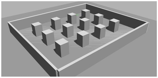
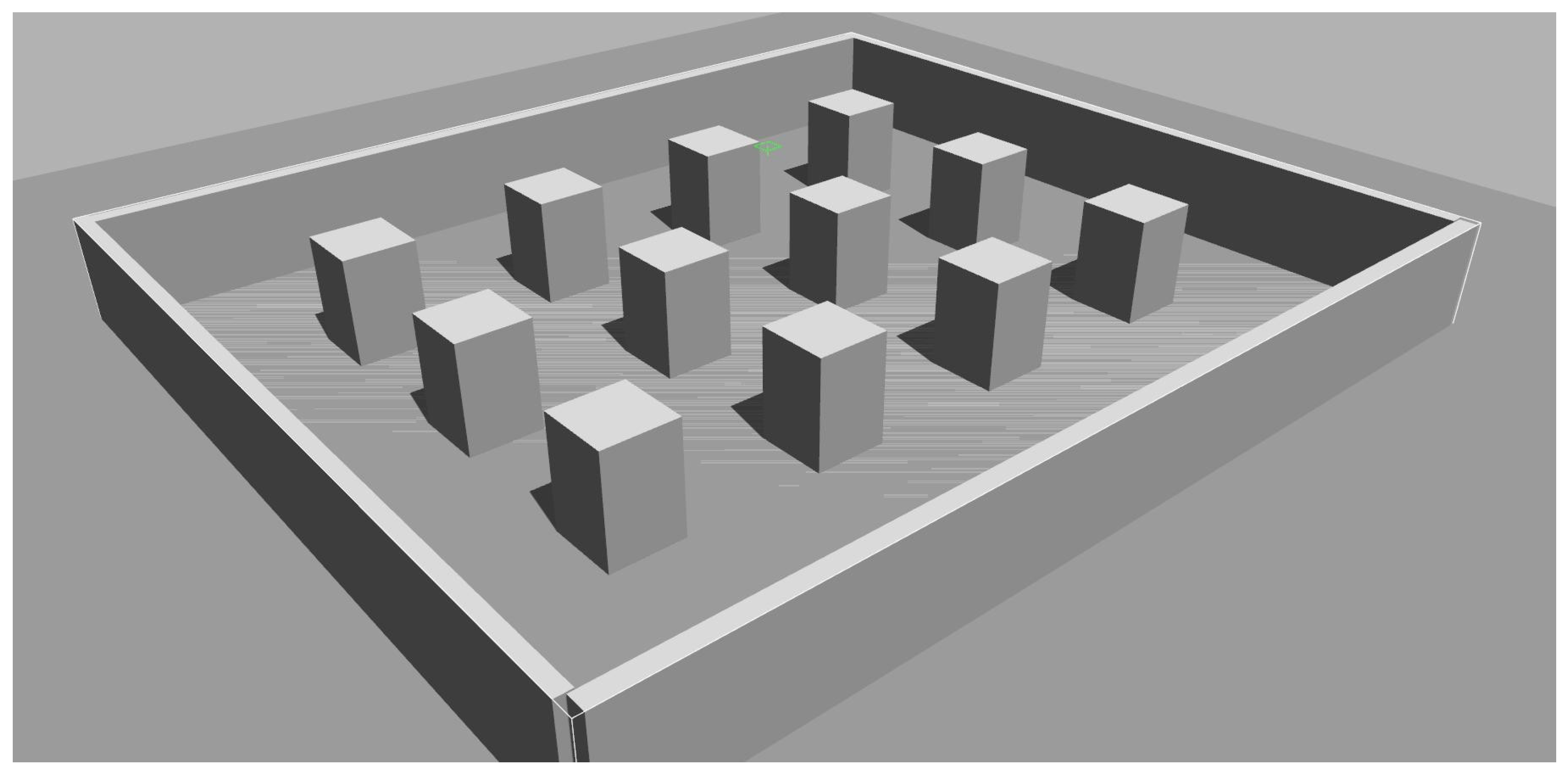
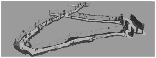
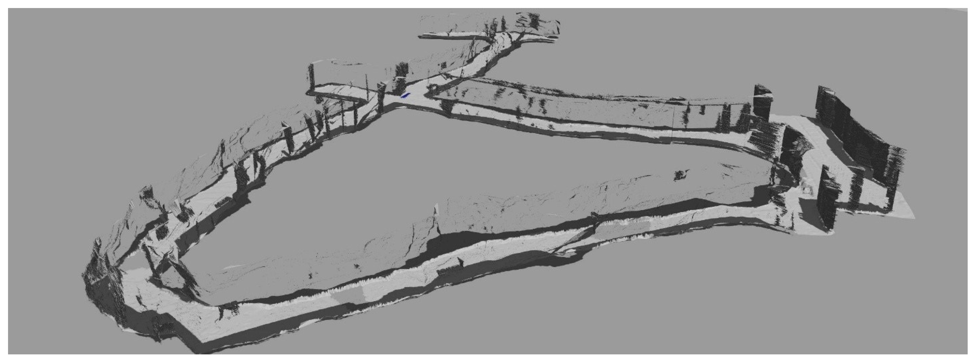
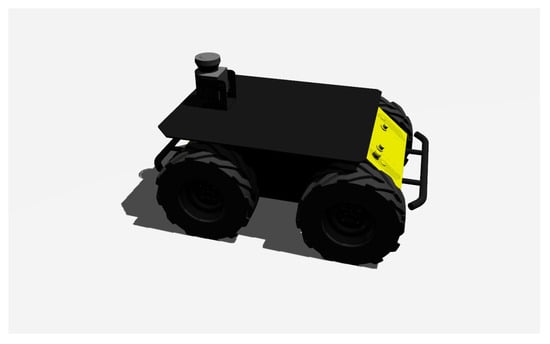
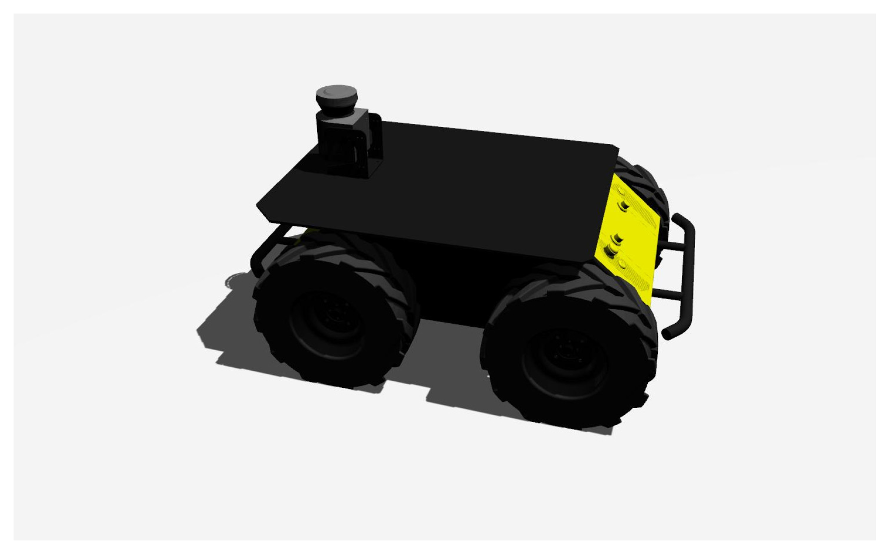
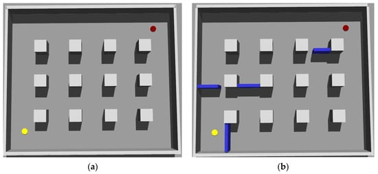
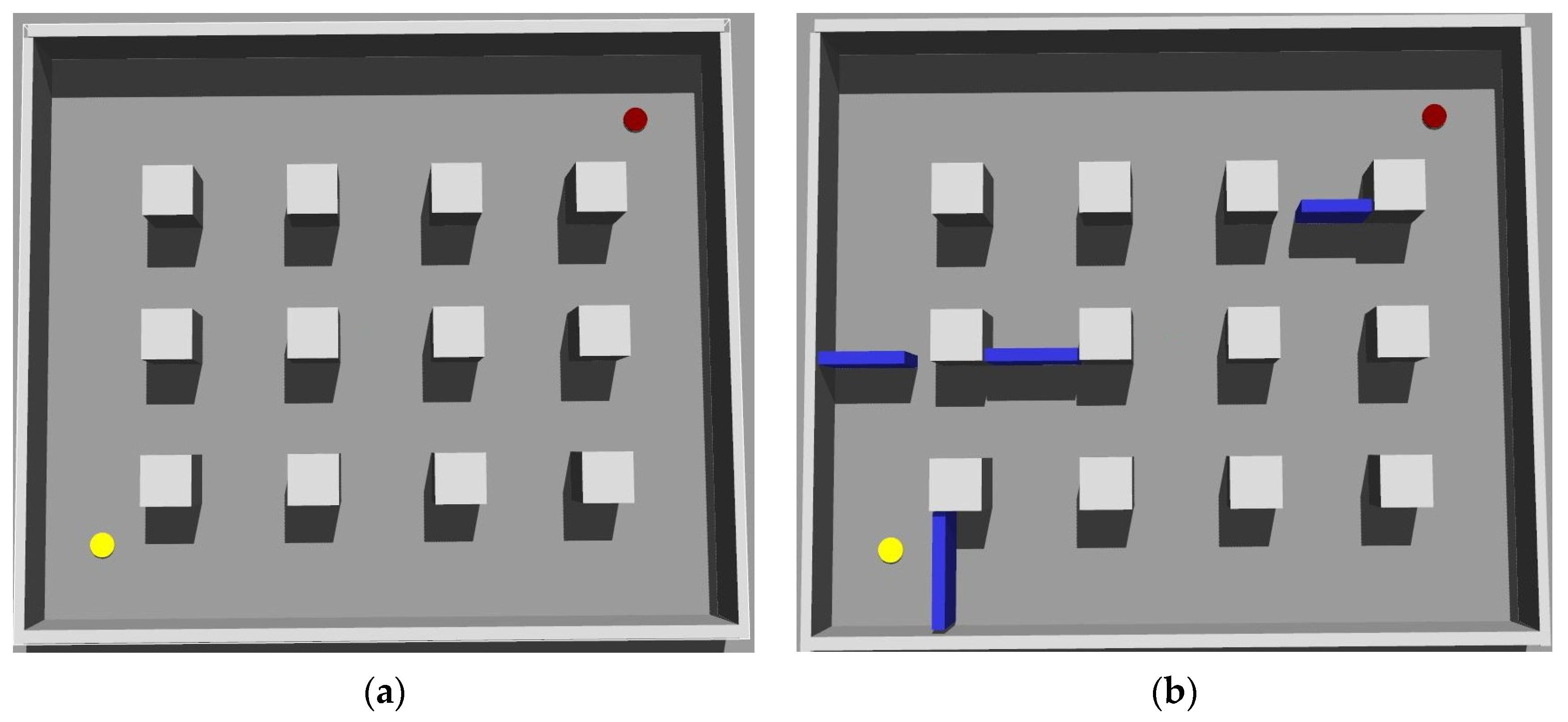
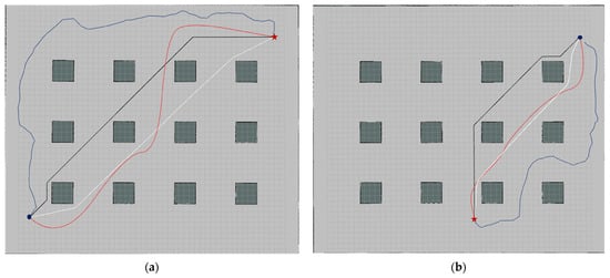
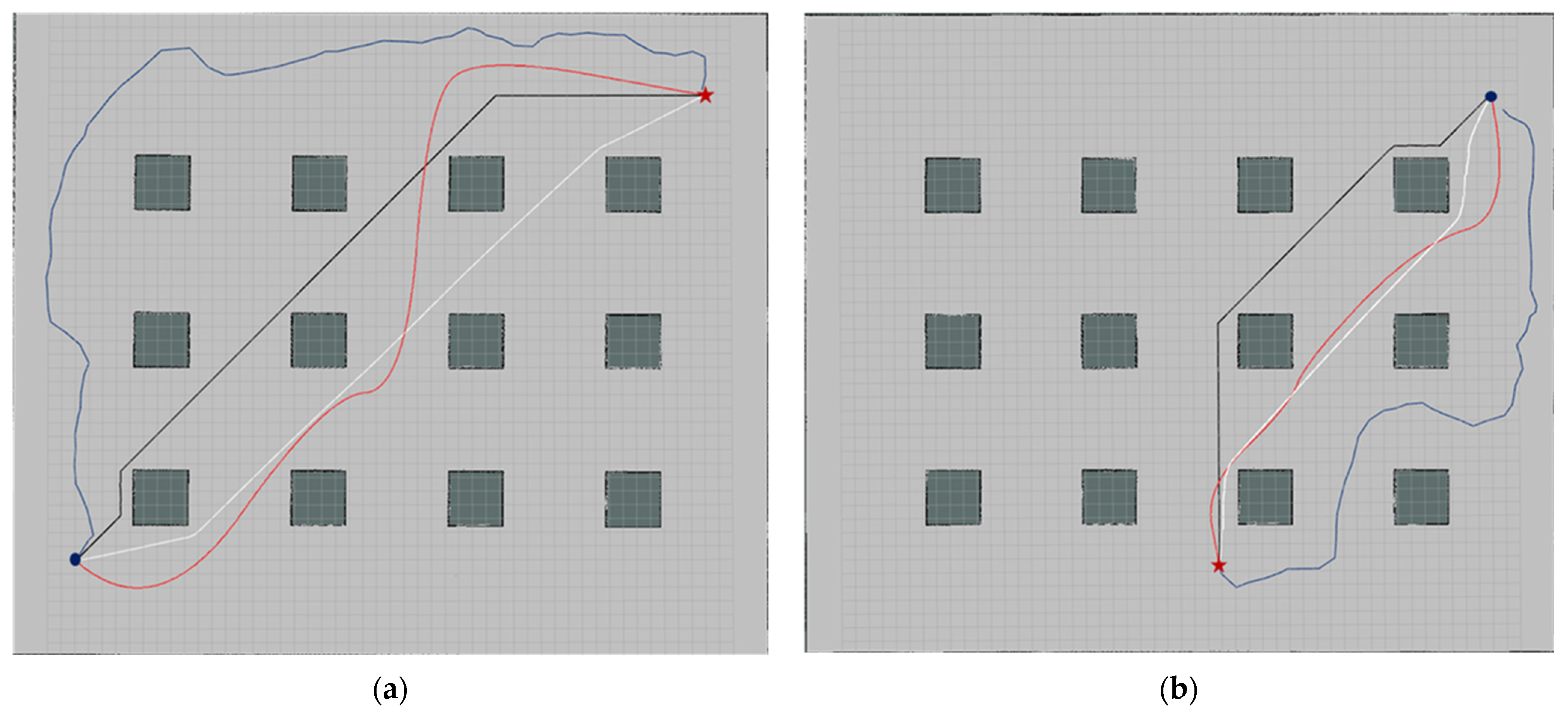
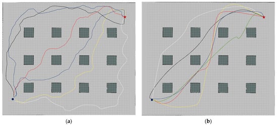
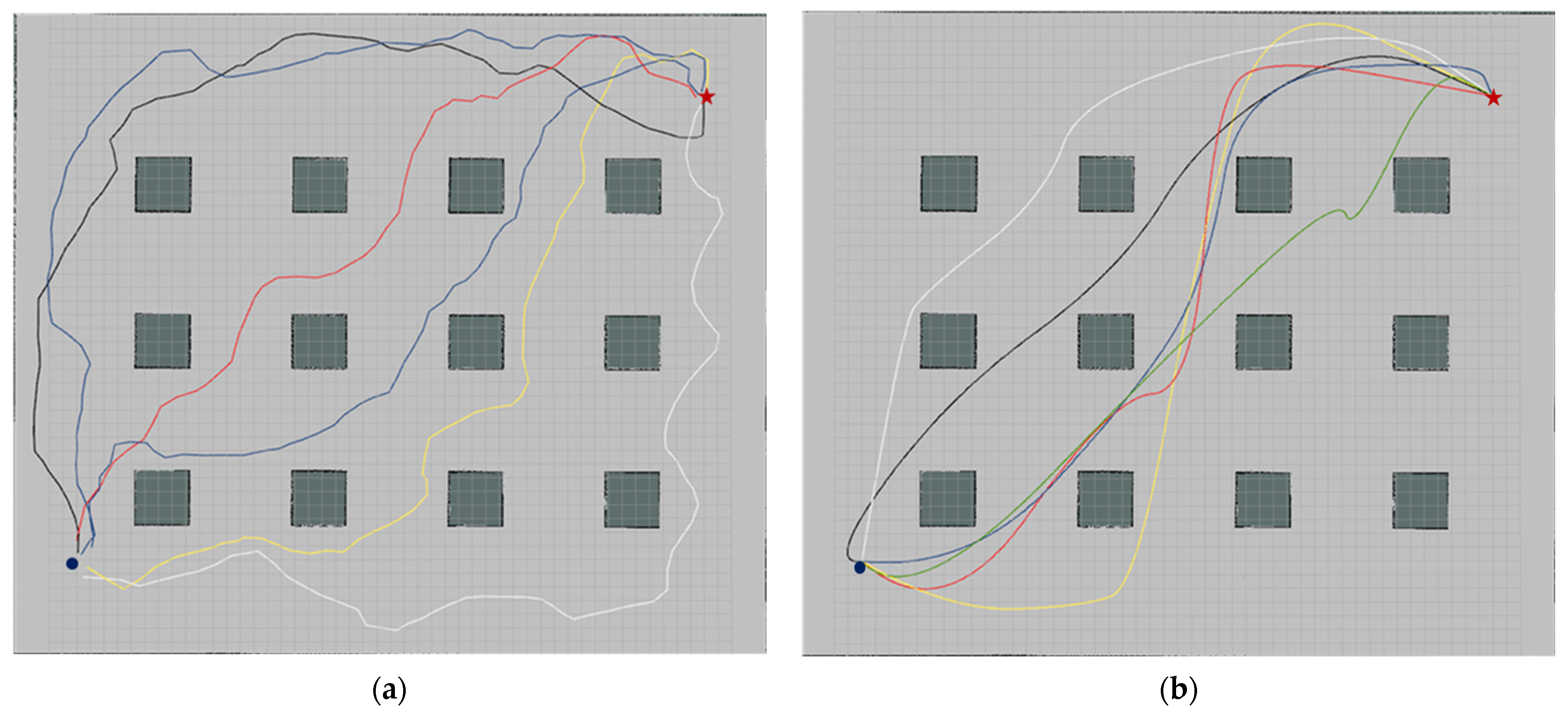
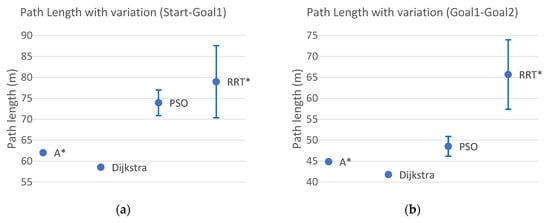
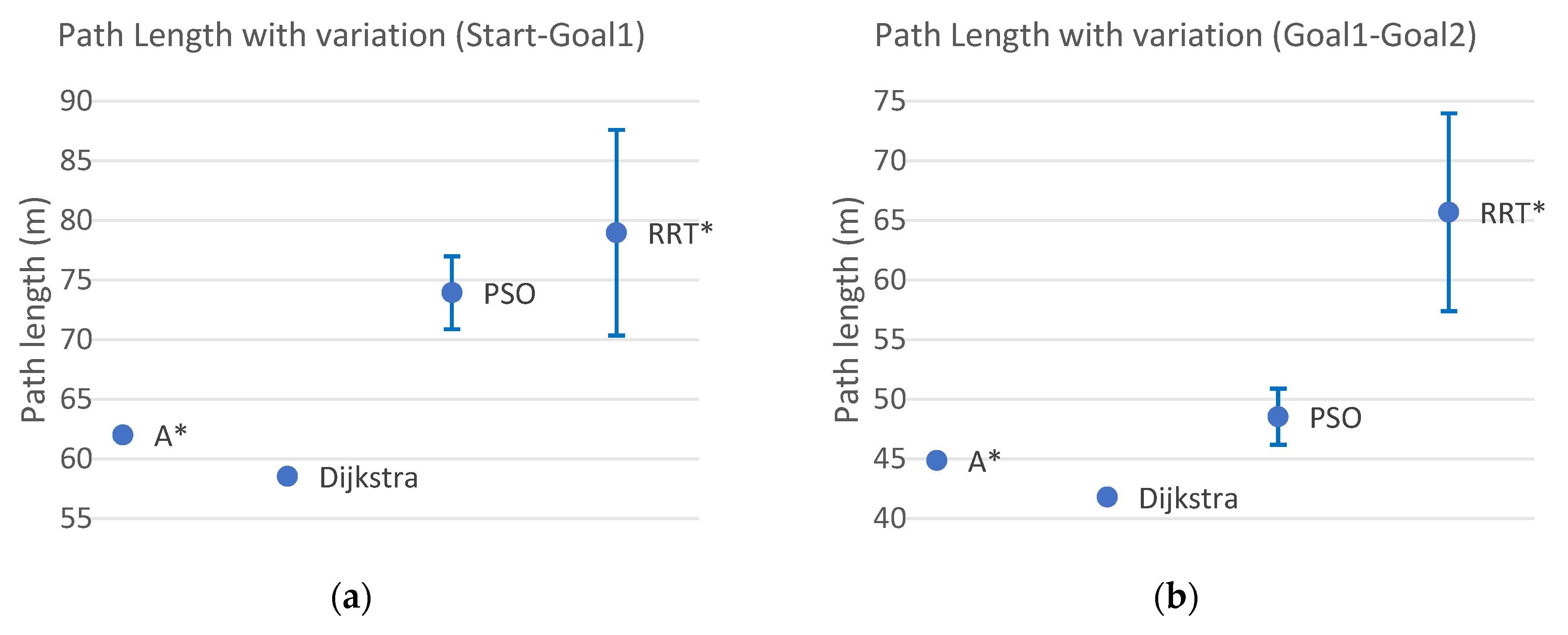
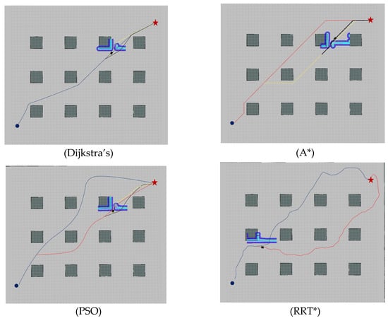
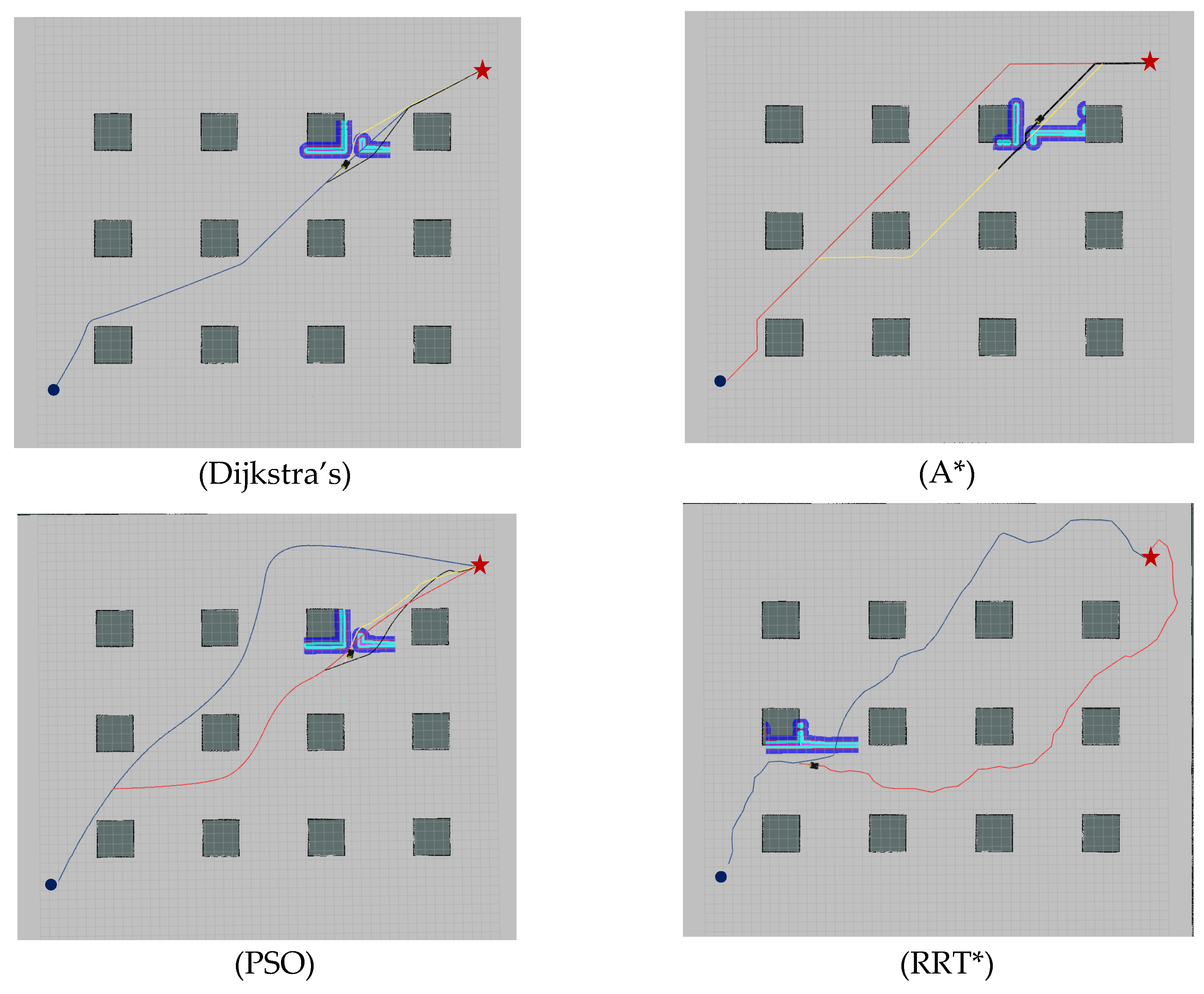
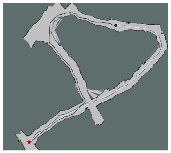
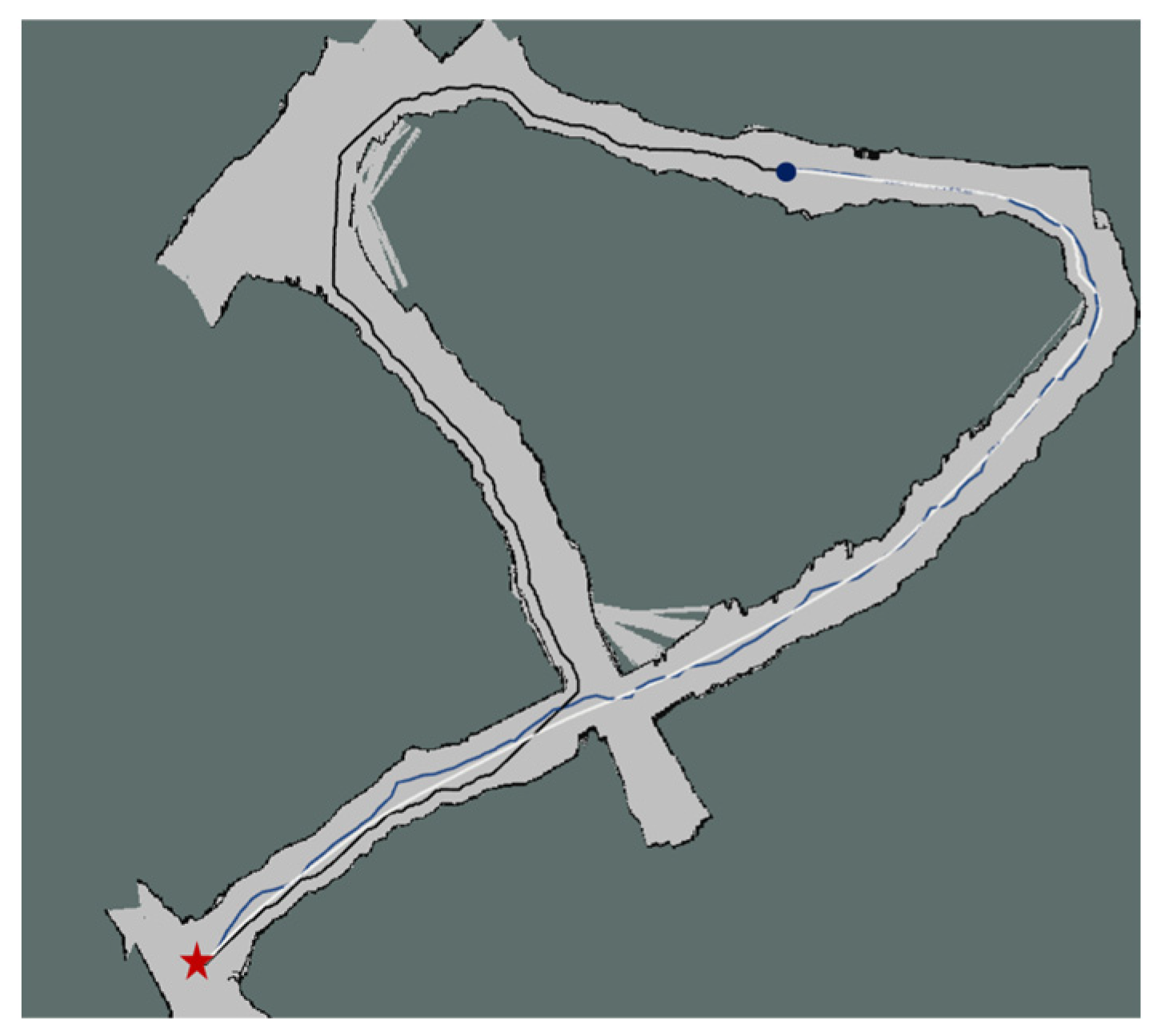
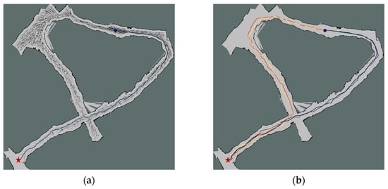
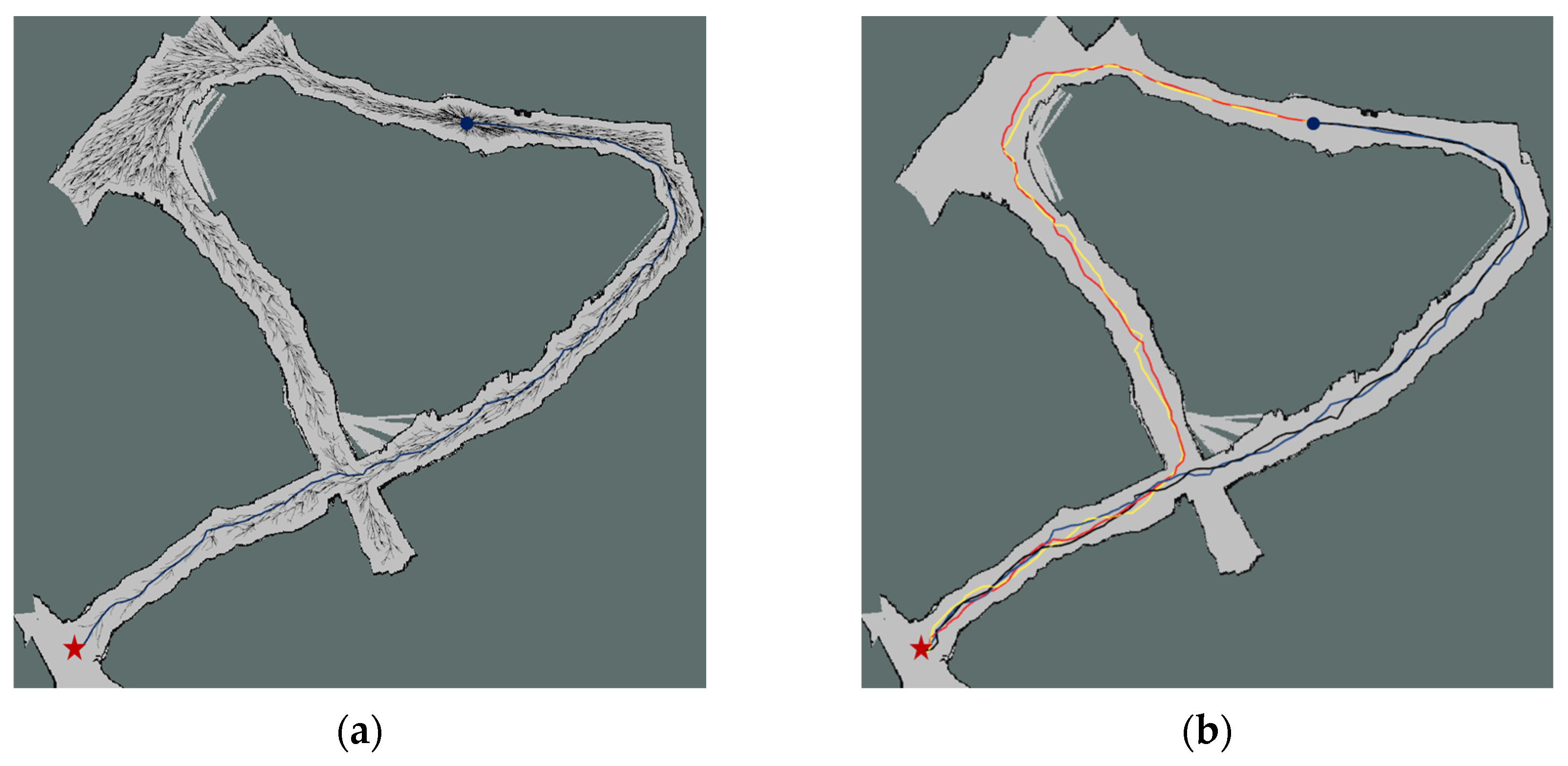
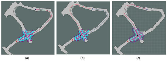
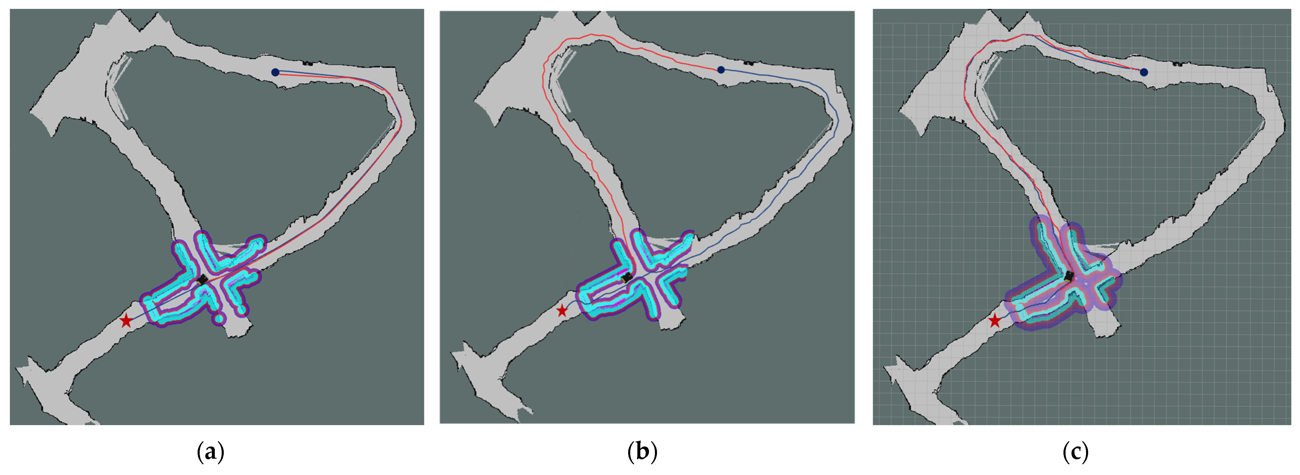
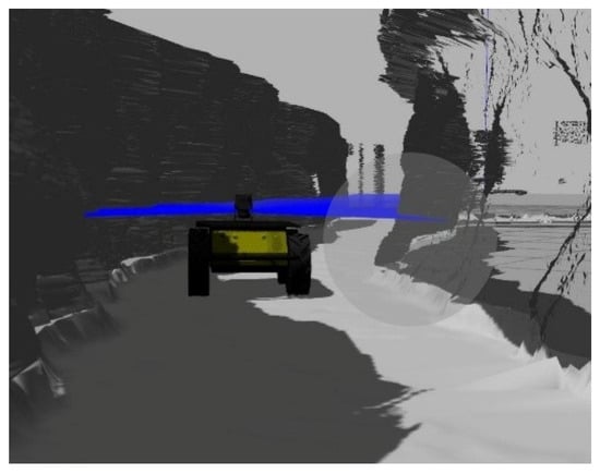
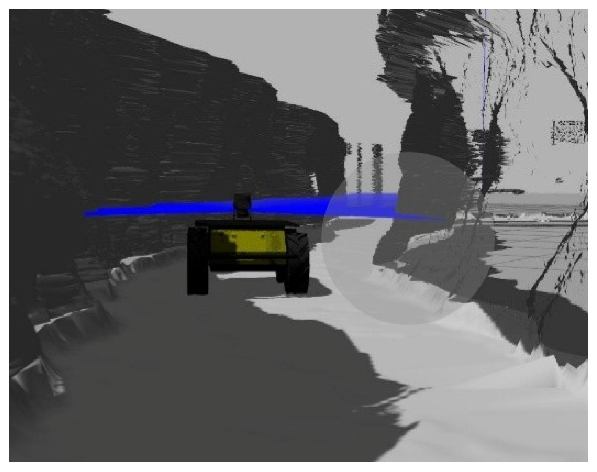

Disclaimer/Publisher’s Note: The statements, opinions and data contained in all publications are solely those of the individual author(s) and contributor(s) and not of MDPI and/or the editor(s). MDPI and/or the editor(s) disclaim responsibility for any injury to people or property resulting from any ideas, methods, instructions or products referred to in the content. |
© 2026 by the authors. Licensee MDPI, Basel, Switzerland. This article is an open access article distributed under the terms and conditions of the Creative Commons Attribution (CC BY) license.