Fragmentation and Vulnerability in the Global Natural Gas Market for a Sample of 59 Countries: A Combined Approach of Econometric Modeling and Hierarchical Clustering

Abstract

This article aims to examine how the natural gas market evolved following the price shocks observed between 2020 and 2024, paying particular attention to market integration and the persistence of these shocks. The proposed analysis uses daily price data for the Title Transfer Facility (TTF), the main European benchmark traded on the Intercontinental Exchange and quoted in EUR/MWh, as well as Henry Hub (HH), the United States benchmark. These series are combined with a country panel on natural gas production, consumption, and gross domestic product for 59 economies, subject to data availability. The cointegration results show that TTF and HH prices moved together in 2019, but this relationship broke down in 2020 and did not return to its previous pattern in the following years. Granger causality tests point to a one-directional transmission from Henry Hub to Europe. Moreover, GARCH estimates indicate that TTF reacts almost twice as strongly to daily shocks as HH, while volatility remains persistent in both markets. Fixed-effects estimates place the TTF price elasticity of import spending close to 0.5, providing evidence consistent with a causal link between higher natural gas prices and higher domestic energy expenditure. Finally, the clustering analysis complements the econometric modeling by identifying four groups of countries defined by gas import dependency and gas intensity. This classification also offers implications for the global natural gas market since it points to the need for cluster-specific policy approaches rather than a single solution applied to every country.

1. Introduction

Natural gas currently accounts for roughly 25 percent of global primary energy demand and plays an important role in the transition away from coal-fired power generation. Because gas trades at the regional level rather than on a single world spot market, as crude oil does, it is not fully integrated across geographic regions. Long-term contracts are typically established between producers and consumers connected by pipeline, while liquefied natural gas (LNG) allows gas to reach new markets but requires costly export and import terminals.

Thus, natural gas integration, the extent to which a price change in one market is transmitted across the other markets, is contingent on spare LNG capacity and contract terms, and on the availability of import terminals in consuming countries. This paper examines whether three major shocks during 2019 to 2024, namely the pandemic, the withdrawal of Russian pipeline gas from Europe, which sent title transfer facility (TTF) prices to a peak above 330 USD/MMBtu, roughly forty times the contemporaneous Henry Hub (HH) quote, and the increase in gas demand from China and Southeast Asia, led to a permanent disruption of natural gas price integration. Throughout the paper, we use the term fragmentation to denote a persistent breakdown of the law of one price between regional benchmarks, that is, a state in which arbitrage no longer ties the two benchmarks together, and the price spread stops reverting to a stable long-run level, as opposed to a temporary deviation that fades once the shock subsides.

The main objectives of this article are set out below: First, this article documents that the HH–TTF price relationship deteriorated during 2020 and has not yet reversed, thus providing evidence of the collapse of the natural gas market during the 2020s to the literature that mostly covers periods prior to the 2020s or focuses on the relationship between oil and natural gas.

Second, this paper also develops an integrated natural gas vulnerability index by combining dependency and gas intensity, identifying four distinct clusters through hierarchical classification, which captures an aspect of exposure that simple import ratios miss: a moderately dependent country with very high gas intensity (Thailand and Kuwait) may face larger welfare losses from a price shock than a highly dependent country whose economy is not gas-intensive (Poland).

Third, we estimate the degree of price pass-through to natural gas importing countries and find that a ten percent increase in the TTF benchmark raises average import expenditure by approximately five percent. This result contributes to the energy security literature by providing evidence consistent with a causal channel running from natural gas price increases to national energy spending, while we discuss below the endogeneity concerns that prevent us from interpreting the estimate as a fully identified causal effect.

The rest of this paper is organized as follows: Section 2 reviews the related literature on gas market integration, the price transmission process, and energy vulnerability, and sets out the conceptual framework; Section 3 presents the data and the empirical strategy; Section 4 reports the results; Section 5 discusses the implications and limitations of the empirical findings; finally, Section 6 concludes.

2. Literature Review

Since the pioneering studies of [1] inquiring whether rising LNG trade was establishing a unified, world-scale gas price, the global linkage of natural gas markets has been a persistent point of concern. While the results of his cointegration tests of HH, the national balancing point (NBP) in the UK, and Asian spot market indexes showed relatively little evidence of price convergence, he suggested the rigidity of destination clauses in long-term LNG supply contracts to be a likely culprit. In this sense, Ref. [2] returned to this issue using an extended sample size and a Kalman filter approach and concluded that global integration had marginally improved but still falls far short of full-blown globalization, with stronger integration in the Atlantic markets than in the Pacific.

Since then, the market has experienced a period of extreme volatility; while the pandemic-induced demand contraction resulted in short-term convergence across markets, the Russia–Ukraine conflict precipitated the most significant supply-side disruption in the history of the European gas markets. On the question of the nature of co-movements between gas markets, Ref. [3] used a copula-based model to explore the risk transmission between oil and gas spot markets and observed that cross-market dependencies are asymmetric and dependent on the risk regime. Indeed, 2022 proved just as [3] warned, as their findings of regime-dependent co-movements and the non-linear nature of the co-movements would have posed challenges to any linear, cointegration-based model of the markets.

In an earlier structural VAR study, Ref. [4] broke down natural gas prices into three distinct components (supply, demand, and speculation) using data on the HH benchmark and found that supply is dominant in the short run and demand matters in the long run. This study does not focus on the back-and-forth between HH and another gas market benchmark, an issue this paper seeks to address by considering both HH and TTF returns in a reduced-form VAR analysis and generating a series of impulse response functions to illustrate the directional flow of information between the two markets.

The idea of energy vulnerability has been present in the literature for some time. Ref. [5] developed a framework divided into sovereignty, robustness, and resilience; they suggest that the metrics should encompass all three concepts. Moreover, in an extensive review of energy security measures, Ref. [6] notes that several indices are essentially conflating energy vulnerability with reliance on imports, and that few studies consider energy intensity for particular fuels.

On the other hand, the method of clustering presented here helps us distinguish vulnerability from reliance on imports; for gas in particular, we can measure exposure in both import dependency and gas intensity. In the case of Latin America, Ref. [7] discusses the dynamic hedging of natural gas prices in Mexico, and the authors find that using a conditional variance model produces better results than a static hedging strategy. However, this method is also more sensitive to short-term shocks, meaning that it requires very short forecast horizons. Likewise, Ref. [8] discusses changes in the prices of gasoline and natural gas brought on by the COVID-19 pandemic in six Latin American economies; they conclude that the changes differed across the economies, and those differences could be largely explained by differences in national policy or exposure to international markets.

Moreover, Ref. [9] looked at input–output tables for raw material trade and used network analysis methods to discuss how a commodity market’s structure depends heavily on existing infrastructure and on how that infrastructure is organized. They suggest that some standard network measures would require additional adjustment to be useful in such an industry.

The works cited above, especially those of [5,9], provide a broader context for this discussion and help us understand how Mexico’s combination of moderate import dependency with high gas intensity fits into the wider picture. There has also been recent discussion on networks related to the global LNG trade. For instance, Ref. [10] maps out a global LNG shipping network, concluding that it has a small-world topology that has become more connected over time. In this sense, Ref. [11] assesses the robustness of the global LNG network from 2013 to 2023, concluding that targeted removal of high betweenness centrality nodes affects network performance more drastically than random removal.

Our paper adds to this discussion by looking at the global gas pricing network, and our work differs significantly from these papers, which address issues of shipping and flows, as opposed to the issues here, which address issues of price differences and returns. Rather than looking at the existence of shipping routes, for example, we look at the adequacy of shipping routes in conveying price information to other markets.

Conceptual Framework

The empirical analysis that follows rests on a single organizing idea. The degree of integration between two regional gas benchmarks reflects the strength of the arbitrage that links them, and that arbitrage can be weakened or severed through four channels. We use these channels to connect the methods applied in Section 3 and Section 4, so that each tool addresses a specific part of the same mechanism rather than standing on its own.

The first channel is the set of LNG arbitrage constraints. When spare liquefaction and regasification capacity is available, cargoes flow from low-price to high-price regions until the price gap narrows to the cost of transport, which keeps the benchmarks cointegrated [12,13]. When that spare capacity is exhausted, the no-arbitrage band widens, and the long-run relationship can disappear, which is what the Engle and Granger cointegration tests in Section 4.2 are designed to detect. The second channel is infrastructure bottlenecks. Pipeline and terminal capacity determine how fast a price signal in one region reaches another, so a shortage of import terminals or the loss of a pipeline route can block transmission even when a price gap remains open [11,14]. The Granger causality tests and the vector autoregression in Section 4.3 measure the direction and speed of this transmission. The third channel is geopolitical risk transmission. Supply interruptions driven by conflict or policy, rather than by fundamentals, raise the conditional volatility of the affected benchmark and can do so asymmetrically across regions [3,15]. The GARCH estimates in Section 4.4 capture this volatility response. The fourth channel is market regime shifts. The relationship between regional benchmarks need not be stable over time, and growing literature models it with structural breaks and regime-switching specifications, precisely because linear models miss the periodic decoupling of gas prices [13,16,17]. The sub-period cointegration tests in Section 4.2 and the variance ratios in Section 4.4 are our reduced-form way of detecting such a shift.

These four channels operate at the level of benchmark prices. To connect them to real economies, we add a country dimension. A given degree of fragmentation translates into different welfare consequences depending on how exposed each economy is to the benchmark price, and that exposure depends jointly on how much gas a country must import and on how gas-intensive its output is. The hierarchical clustering in Section 4.5 groups countries by this combined exposure, and the panel regression in Section 4.6 quantifies how strongly benchmark prices pass through into national import bills. The clustering is, therefore, not a separate exercise. It identifies the groups of countries for which the price transmission documented in the earlier sections matters most, and the panel estimate gives the average size of that transmission. Whether the convergence observed before 2020 has given way to a lasting divergence is, within this framework, an empirical question as to which of the four channels comes to dominate [18].

3. Data and Methods

3.1. Price Data

We collect the daily closing prices of two gas benchmark contracts between 2 January 2019 and 31 December 2024, resulting in 1510 aligned trading days. Benchmark 1 is the HH front-month futures contract (NYMEX NG=F), which is denominated in US dollars per million British thermal units (MMBtu) and represents the gas benchmark for gas production in North America. In addition, HH also determines the implicit price floor for US LNG exports. In other words, the HH price is a critical component in the determination of the LNG export price. Benchmark 2 is the TTF front-month futures contract quoted in MMBtu (after conversion from the native currency and unit denomination of EUR/MWh using the daily exchange rates).

The TTF has become the main price benchmark for the European gas market since the mid-2010s. Prior to this time, the UK’s National Balancing Point (NBP) was the prevailing benchmark for European pricing. HH averaged USD 3.33 MMBtu (with a standard deviation of USD 1.74 MMBtu) while TTF averaged USD 46.79 MMBtu (with a standard deviation of USD 48.39 MMBtu). The spread between the two gas benchmarks ranges from a minimum of USD 1.68 MMBtu in mid-2020 to a maximum of USD 329.90 MMBtu in August 2022. For our econometric analysis, we use log-prices and log-returns for each benchmark defined as:

$${\mathrm{p}}_{\mathrm{t}}^{\mathrm{H}\mathrm{H}}=\mathrm{l}\mathrm{n}\left({\mathrm{P}}_{\mathrm{t}}^{\mathrm{H}\mathrm{H}}\right),{\mathrm{p}}_{\mathrm{t}}^{\mathrm{T}\mathrm{T}\mathrm{F}}=\mathrm{l}\mathrm{n}\left({\mathrm{P}}_{\mathrm{t}}^{\mathrm{T}\mathrm{T}\mathrm{F}}\right)$$

(1)

$${\mathrm{r}}_{\mathrm{t}}^{\mathrm{H}\mathrm{H}}=\Delta {\mathrm{p}}_{\mathrm{t}}^{\mathrm{H}\mathrm{H}}={\mathrm{p}}_{\mathrm{t}}^{\mathrm{H}\mathrm{H}}-{\mathrm{p}}_{\mathrm{t}-1}^{\mathrm{H}\mathrm{H}},{\mathrm{r}}_{\mathrm{t}}^{\mathrm{T}\mathrm{T}\mathrm{F}}=\Delta {\mathrm{p}}_{\mathrm{t}}^{\mathrm{T}\mathrm{T}\mathrm{F}}={\mathrm{p}}_{\mathrm{t}}^{\mathrm{T}\mathrm{T}\mathrm{F}}-{\mathrm{p}}_{\mathrm{t}-1}^{\mathrm{T}\mathrm{T}\mathrm{F}}$$

(2)

and the transatlantic log price spread is given by

$${\mathrm{s}}_{\mathrm{t}}=\mathrm{l}\mathrm{n}\left({\displaystyle \frac{{\mathrm{P}}_{\mathrm{t}}^{\mathrm{T}\mathrm{T}\mathrm{F}}}{{\mathrm{P}}_{\mathrm{t}}^{\mathrm{H}\mathrm{H}}}}\right)={\mathrm{p}}_{\mathrm{t}}^{\mathrm{T}\mathrm{T}\mathrm{F}}-{\mathrm{p}}_{\mathrm{t}}^{\mathrm{H}\mathrm{H}}$$

(3)

3.2. Country-Level Panel Data

We use natural gas production and consumption data on 59 countries for the period 2019 to 2024 from [19]. Gross domestic products in current US dollars and per capita are taken from [20]. Trade data for HS 271111 LNG and HS 271121 (pipeline gas) comes from the preview API of [21], which returns reporter-to-world aggregates rather than bilateral-level trade data.

Table 1 shows the complete sample of countries, divided into groups by their primary role in the gas market. The division is based on the net export/consumption ratio in the last year for which the data on both production and consumption are available: countries in which production exceeds consumption by over 30% are classified as net exporters, those in which consumption exceeds production by over 30% are classified as net importers, while others are categorized as balanced. 25 countries are missing production or consumption data in the last year of the sample, and so cannot be classified on these lines, although a number of these (Japan, South Korea, France, Spain, and Turkey) are known to be net importers for which the Energy Institute did not produce production figures for 2024. The 59 countries comprise 19 that report both import and export values through Comtrade and constitute the subset used in the panel regression of Section 4.6. This panel is unbalanced: Qatar has data only for 2019, and Russia only up to 2021.

Table 1. Country Classification by Trade Balance.

Panel A. Net Exporters (12 Countries)			Panel C. Net Importers (11 Countries)
Acronym	Country	Trade Data	Acronym	Country	Trade Data
DZA	Algeria	Yes	CHN	China	Yes
AUS	Australia	Yes	DEU	Germany	Yes
CAN	Canada	Yes	IND	India	No
IDN	Indonesia	Yes	IRQ	Iraq	No
ISR	Israel	No	ITA	Italy	Yes
MYS	Malaysia	Yes	KWT	Kuwait	No
NOR	Norway	No	MEX	Mexico	Yes
OMN	Oman	Yes	NLD	Netherlands	Yes
QAT	Qatar	Yes	POL	Poland	No
RUS	Russia	Yes	THA	Thailand	Yes
TTO	Trinidad and Tobago	Yes	GBR	United Kingdom	Yes
TKM	Turkmenistan	No
Panel B. Balanced (11 countries)			Panel D. Classification unavailable (25 countries)
Acronym	Country	Trade data	Acronym	Country	Trade data
ARG	Argentina	Yes	AGO	Angola	FRA
BGD	Bangladesh	No	AUTaqu	Austria	GRC
BRA	Brazil	Yes	BHR	Bahrain	HUN
EGY	Egypt	No	BEL	Belgium	JPN
IRN	Iran	No	BRN	Brunei	JOR
PAK	Pakistan	No	BGR	Bulgaria	LBN
ROU	Romania	No	CHL	Chile	MOZ
SAU	Saudi Arabia	No	CZE	Czechia	TUR
ARE	United Arab Emirates	Yes	Country	ISO3	Country
USA	United States	No	France	NGA	Nigeria
UZB	Uzbekistan	No	Greece	PNG	Papua New Guinea
			Hungary	PRT	Portugal
			Japan	SGP	Singapore
			Jordan	SVK	Slovakia
			Lebanon	KOR	South Korea
			Mozambique	ESP	Spain

Source: authors’ elaboration based on data from the Energy Institute [19], the World Bank [20], and the UN Comtrade database [21]. Notes: The “Trade data” variable denotes whether the country includes import or export values for HS 271111 and HS 271121 in the UN Comtrade preview API. A country is classified as a net exporter when its production exceeds consumption by more than 30 percent; a country is classified as a net importer when consumption exceeds production by the same margin. Panel D countries do not have production or consumption data for the most recent year available for the Energy Institute source, so they could not be classified as net importers or net exporters.

3.3. Econometric Methodology

Unit root and cointegration tests. The augmented Dickey–Fuller (ADF) stationarity test, selecting its lag length automatically via the Akaike information criterion (AIC), is used to assess the stationarity of the logarithmic price series. The ADF regression takes the form:

$$\Delta {\mathrm{x}}_{\mathrm{t}}=\mathsf{\mu }+\mathsf{\varphi }{\mathrm{x}}_{\mathrm{t}-1}+{\displaystyle \sum _{\mathrm{i}=1}^{\mathrm{k}}}{\mathsf{\gamma }}_{\mathrm{i}}\Delta {\mathrm{x}}_{\mathrm{t}-\mathrm{i}}+{\mathsf{\epsilon }}_{\mathrm{t}}$$

(4)

$${\mathrm{H}}_0:\mathsf{\varphi }=0$$

(5)

where the null hypothesis H₀: ϕ = 0 implies a unit root. Lag length k is selected by the AIC. Once the series is found to be I(1), the Engle–Granger cointegration test is applied in a two-step procedure, first estimating the long-run relationship:

$${\mathrm{p}}_{\mathrm{t}}^{\mathrm{T}\mathrm{T}\mathrm{F}}=\mathsf{\alpha }+\mathsf{\beta }{\mathrm{p}}_{\mathrm{t}}^{\mathrm{H}\mathrm{H}}+{\mathrm{u}}_{\mathrm{t}}$$

(6)

and then testing whether the residuals ûₜ are stationary by running the auxiliary regression:

$$\Delta {\widehat{\mathrm{u}}}_{\mathrm{t}}=\mathsf{\rho }{\widehat{\mathrm{u}}}_{\mathrm{t}-1}+{\displaystyle \sum _{\mathrm{i}=1}^{\mathrm{k}}}{\theta }_{\mathrm{i}}\Delta {\widehat{\mathrm{u}}}_{\mathrm{t}-\mathrm{i}}+{\mathsf{\eta }}_{\mathrm{t}}$$

(7)

covering sub-samples defined by the major structural events: 2019 (pre-COVID), 2020 (COVID), 2021 (recovery), 2022 (the Russia crisis), and 2023 to 2024 (post-crisis).

We adopt an operational definition of fragmentation that combines two observable conditions. A pair of regional benchmarks is integrated when their log prices are cointegrated, so that the transatlantic spread is stationary and reverts to a stable mean, and when arbitrage keeps that spread inside a band set by transport costs. We classify the market as fragmented when both conditions fail at the same time, that is, when cointegration is absent, and the spread itself contains a unit root, since a non-stationary spread implies that any gap between the two benchmarks can persist or widen with no tendency to close. This definition separates structural fragmentation from a transitory deviation. A short-lived volatility episode raises the spread temporarily but leaves the long-run relationship intact, so cointegration survives, and the spread reverts once the shock passes. Persistent fragmentation, by contrast, requires the breakdown to hold across consecutive sub-periods rather than in a single crisis year. We, therefore, test cointegration year by year and treat the combined evidence from the sub-period tests, the unit-root test on the spread, and the rolling return correlation as the basis for the classification, rather than relying on any single statistic. A regime-switching model, such as a Markov-switching specification, provides a sharper statistical characterization of the transition between regimes, and we report such a model as a robustness check in Section 4.8.

Granger Causality and VAR Tests

A series of pairwise Granger causality tests on logarithmic returns is computed with 1 to 5 lags. We fit a vector autoregression (VAR) to the two-dimensional log-return series, with order p selected by AIC among ten alternative specifications:

$${\mathrm{r}}_{\mathrm{t}}=\mathrm{c}+{\displaystyle \sum _{\mathrm{i}=1}^{\mathrm{p}}}{\mathrm{A}}_{\mathrm{i}}{\mathrm{r}}_{\mathrm{t}-\mathrm{i}}+{\mathsf{\epsilon }}_{\mathrm{t}}$$

(8)

where ${\mathrm{r}}_{\mathrm{t}}$ is the log-return. In this case, HH Granger causes TTF if the null hypothesis H₀: a_12,1 = a_12,2 = ⋯ = a_12,p = 0 is rejected. Impulse response functions from the Wold moving-average representation:

$${\mathrm{r}}_{\mathrm{t}}=\mathsf{\mu }+{\displaystyle \sum _{\mathrm{h}=0}^{\mathrm{\infty }}}{\Psi }_{\mathrm{h}}{\mathsf{\epsilon }}_{\mathrm{t}-\mathrm{h}}$$

(9)

capture the response of each variable to a one-standard-deviation shock in the other over a 20-day window. GARCH-based estimates of volatility. Moreover, a univariate GARCH(1, 1) model with Student-t innovations is fitted to each return series to capture the excess kurtosis characteristic of energy data:

$${\mathrm{r}}_{\mathrm{t}}=\mathsf{\mu }+{\mathsf{\epsilon }}_{\mathrm{t}},\hspace{1em}{\mathsf{\epsilon }}_{\mathrm{t}}={\mathsf{\sigma }}_{\mathrm{t}}{\mathrm{z}}_{\mathrm{t}},\hspace{1em}{\mathrm{z}}_{\mathrm{t}}~{\mathrm{t}}_{\mathsf{\nu }}(0,1)$$

(10)

$${\mathsf{\sigma }}_{\mathrm{t}}^2=\mathsf{\omega }+\mathsf{\alpha }{\mathsf{\epsilon }}_{\mathrm{t}-1}^2+\mathsf{\beta }{\mathsf{\sigma }}_{\mathrm{t}-1}^2$$

(11)

The parameter α is the ARCH coefficient (sensitivity of conditional variance to daily shocks), β is the GARCH coefficient (persistence), and their sum α + β measures how slowly volatility reverts to its unconditional level. As a descriptive measure of rolling co-movement, we also compute the 60-day window return correlation:

$${\mathsf{\rho }}_{\mathrm{t}}^{\left(60\right)}=\mathrm{C}\mathrm{o}\mathrm{r}\mathrm{r}\left({\mathrm{r}}_{\mathrm{t}-59:\mathrm{t}}^{\mathrm{H}\mathrm{H}},{\mathrm{r}}_{\mathrm{t}-59:\mathrm{t}}^{\mathrm{T}\mathrm{T}\mathrm{F}}\right)$$

(12)

Finally, the correlation between the GARCH-standardized residuals serves as an estimate of the dynamic conditional correlation of the two series.

Estimating vulnerability indicators. For each country and each year, we calculate two measures of economic vulnerability. Import dependency is defined as the share of gas consumption covered by net imports:

$${\mathrm{I}\mathrm{m}\mathrm{p}\mathrm{o}\mathrm{r}\mathrm{t}\mathrm{D}\mathrm{e}\mathrm{p}}_{\mathrm{i}\mathrm{t}}={\displaystyle \frac{{\mathrm{C}\mathrm{o}\mathrm{n}\mathrm{s}}_{\mathrm{i}\mathrm{t}}-{\mathrm{P}\mathrm{r}\mathrm{o}\mathrm{d}}_{\mathrm{i}\mathrm{t}}}{{\mathrm{C}\mathrm{o}\mathrm{n}\mathrm{s}}_{\mathrm{i}\mathrm{t}}}}.$$

(13)

Here, the theoretical range is [−1, 1], where −1 indicates a pure exporter, 1 means total import dependence, and 0 denotes a balanced producer-consumer.

The second indicator, gas intensity, measures gas consumption per unit of GDP:

$${\mathrm{G}\mathrm{a}\mathrm{s}\mathrm{I}\mathrm{n}\mathrm{t}\mathrm{e}\mathrm{n}\mathrm{s}\mathrm{i}\mathrm{t}\mathrm{y}}_{\mathrm{i}\mathrm{t}}={\displaystyle \frac{{\mathrm{C}\mathrm{o}\mathrm{n}\mathrm{s}}_{\mathrm{i}\mathrm{t}}}{{\mathrm{G}\mathrm{D}\mathrm{P}}_{\mathrm{i}\mathrm{t}}}}$$

(14)

where ${\mathrm{C}\mathrm{o}\mathrm{n}\mathrm{s}}_{\mathrm{i}\mathrm{t}}$ is in TWh and ${\mathrm{G}\mathrm{D}\mathrm{P}}_{\mathrm{i}\mathrm{t}}$ is in billions of USD. To identify countries with similar vulnerability profiles, we group them using hierarchical clustering. Variables are standardized before clustering:

$${\mathrm{z}}_{\mathrm{i}\mathrm{k}}={\displaystyle \frac{{\mathrm{x}}_{\mathrm{i}\mathrm{k}}-{\overline{\mathrm{x}}}_{\mathrm{k}}}{{\mathrm{s}}_{\mathrm{k}}}}$$

(15)

Clusters are then formed by Ward’s minimum-variance linkage, which at each step merges the pair (A, B) that minimizes the increase in total within-cluster variance given by:

$$\Delta \left(\mathrm{A},\mathrm{B}\right)={\displaystyle \frac{{\mathrm{n}}_{\mathrm{A}}{\mathrm{n}}_{\mathrm{B}}}{{\mathrm{n}}_{\mathrm{A}}+{\mathrm{n}}_{\mathrm{B}}}}{‖{\overline{\mathrm{z}}}_{\mathrm{A}}-{\overline{\mathrm{z}}}_{\mathrm{B}}‖}^2$$

(16)

The procedure is carried out on four standardized features: import dependency, gas intensity, log GDP per capita, and log consumption.

For the panel regression, the effect of gas prices on import expenditure is estimated with the following fixed-effects equation:

$$\ln \left({\mathrm{I}\mathrm{m}\mathrm{p}\mathrm{o}\mathrm{r}\mathrm{t}\mathrm{s}}_{\mathrm{i}\mathrm{t}}\right)={\mathsf{\alpha }}_{\mathrm{i}}+{\mathsf{\beta }}_1\ln \left({\mathrm{G}\mathrm{D}\mathrm{P}}_{\mathrm{i}\mathrm{t}}\right)+{\mathsf{\beta }}_2{\mathrm{I}\mathrm{m}\mathrm{p}\mathrm{o}\mathrm{r}\mathrm{t}\mathrm{D}\mathrm{e}\mathrm{p}}_{\mathrm{i}\mathrm{t}}+{\mathsf{\beta }}_3\ln \left({\mathrm{T}\mathrm{T}\mathrm{F}}_{\mathrm{t}}\right)+{\mathsf{\epsilon }}_{\mathrm{i}\mathrm{t}}$$

(17)

where ${\mathsf{\alpha }}_{\mathrm{i}}$ are country fixed effects that absorb time-invariant heterogeneity in infrastructure, geography, and contracts. Standard errors are clustered at the entity level to allow for serial correlation within countries. The TTF benchmark is introduced as a yearly average, consistent with the frequency of the trade statistics.

Two features of this design support a causal interpretation of the price coefficient, although neither delivers full identification. First, the TTF benchmark is a European market price set by aggregate supply and demand in the continental market. For all but the largest importers in the sample, a single country accounts for a small share of that market, so the annual TTF average is plausibly exogenous to the import bill of any individual economy, which limits the scope for reverse causation from a country to the benchmark. Second, a country’s fixed effects remove every time-invariant determinant of the import bill, such as the stock of regasification capacity, geographic distance to suppliers, and the structure of legacy contracts, so the coefficient is identified from year-to-year movements in price within each country rather than from cross-country differences. We, nonetheless, flag two limitations that prevent us from reading the estimate as a fully identified causal effect. Volumes and prices are jointly determined within a year, so a contemporaneous demand shock could move both the TTF price and the import bill, and the largest importers could in principle exert some influence on the benchmark. We address the first concern in part with the first-differenced and lagged specifications reported in Section 4.7 and Section 4.9, which leave the elasticity in the same range, and we report in Section 4.9 an attempt to instrument the benchmark price with its lag, which turns out to be weakly identified given the short annual price series. We, therefore, interpret the coefficient as a robust conditional pass-through that is consistent with a causal channel, rather than as a point-identified causal parameter.

4. Results

4.1. Unit Roots and the Order of Integration

The augmented Dickey–Fuller tests are shown in Table 2. The null hypothesis of a unit root in levels cannot be rejected by either log price series (HH p-value: 0.38; TTF p-value: 0.69). On the other hand, the unit root hypothesis can be decisively rejected when applied to the first differences (p-value in both cases is less than 0.001).

Table 2. Augmented Dickey–Fuller unit root tests.

Variable	ADF Statistic	p-Value	Lags	Result
ln(HH) [levels]	−1.808	0.377	1	Unit root
ln(HH) [Δ]	−43.050	0	0	Stationary
ln(TTF) [levels]	−1.168	0.687	5	Unit root
ln(TTF) [Δ]	−17.245	0	4	Stationary
ln(TTF/HH) [levels]	−1.746	0.408	9	Unit root
ln(TTF/HH) [Δ]	−14.503	0	8	Stationary

Source: authors’ calculations based on daily Henry Hub futures prices from NYMEX and TTF futures prices from ICE.

The log spread also cannot be shown to be stationary in its level form (p = 0.41); however, the p-value associated with the first difference of the spread implies that we can reject the unit root null hypothesis. As the spread is integrated of order one I(1), this means that the size of the premium that Europe pays over the US benchmark is not mean reverting; the first indication is that there may not be a stable long-run relationship between the two markets over the whole sample.

4.2. Cointegration and Market Fragmentation

Table 3 reports the Engle–Granger cointegration test, broken down by sub-periods. The test statistic for the complete sample is −3.260 (p = 0.061), just missing the five percent rejection region. The sub-period results help explain this outcome. The 2019 period shows strong cointegration between the two benchmarks (EG test statistic = −4.286, p = 0.003), indicating that, notwithstanding certain frictions, the arbitrage forces connecting U.S. LNG exports with European spot prices were still active. This link was disrupted with the advent of the global COVID-19 pandemic.

Table 3. Engle–Granger cointegration tests by sub-period.

Period	N	EG Statistic	p-Value	Result
Full sample (2019–2024)	1510	−3.260	0.061	Not cointegrated
Pre-COVID (2019)	252	−4.286	0.003	Cointegrated
COVID (2020)	253	−2.726	0.19	Not cointegrated
Recovery (2021)	252	−2.156	0.447	Not cointegrated
Russia crisis (2022)	251	−2.564	0.252	Not cointegrated
Post-crisis (2023–2024)	502	−3.216	0.067	Not cointegrated

Source: authors’ calculations based on daily Henry Hub (NYMEX) and TTF (ICE) futures prices.

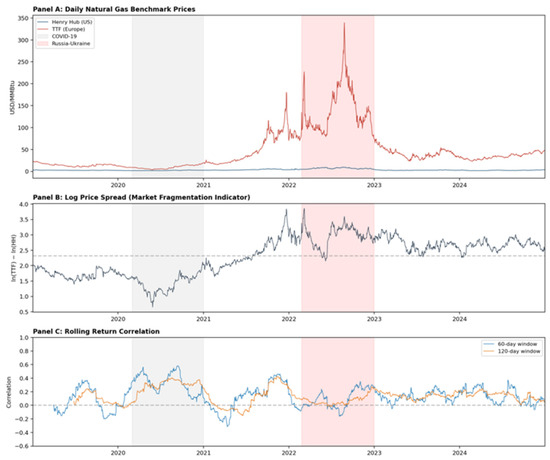
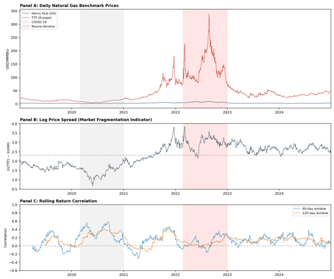
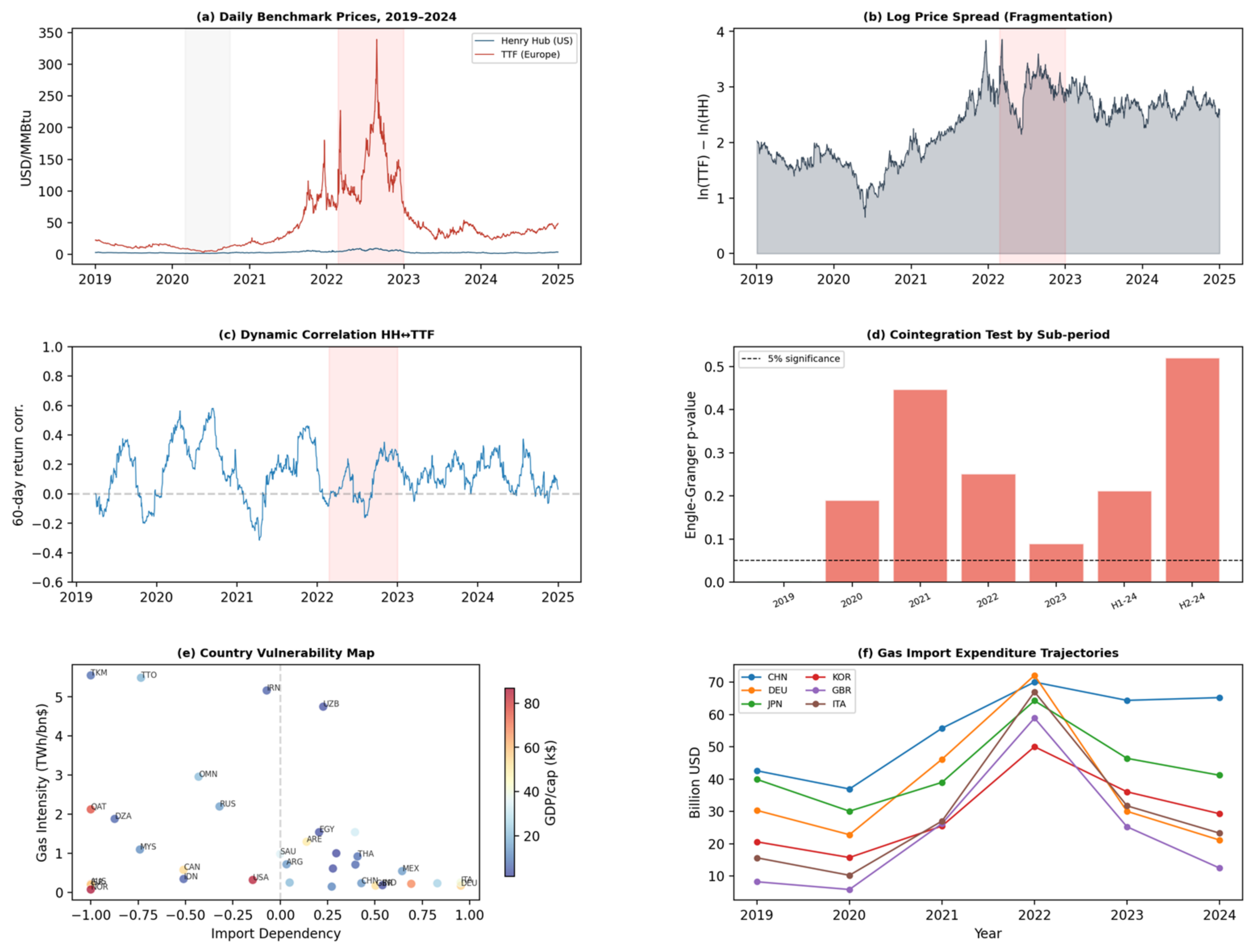
As shown in Table 3, we fail to reject the null of no cointegration between HH and TTF at any meaningful level in the period covering 2020, 2021, and 2022. The post-crisis period of 2023 to 2024 continues to show no evidence of re-convergence (p = 0.067 and 0.52 for the first and second halves of 2024, respectively). Figure 1 depicts this result. Panel A shows the daily benchmark prices. The prices clearly diverged in the 2021 to 2022 period, with TTF rising sharply while HH remained comparatively stable. Panel B shows the corresponding logarithmic spread of the benchmark prices.

Figure 1. Price dynamics. Source: authors’ elaboration based on daily Henry Hub (NYMEX) and TTF (ICE) futures prices.

The log spread increases steadily from a normal value around 1.5, reaches a peak above 3.5, and has yet to return to its pre-COVID value of 1.5. Panel C shows the rolling return correlation of the two series over a 60-day window. The correlation starts around 0.4 and then drops toward zero, at times reaching −0.3, so there are long periods in which the two series are essentially uncorrelated.

4.3. Granger Causality and Impulse Responses

The Granger causality results shown in Table 4 reveal that HH returns cause TTF returns at the one percent level (1 and 2 lags, F = 9.69, p = 0.002 and F = 5.13, p = 0.006), marginally significant at the 5 lag. On the other hand, TTF has no significant causality effect for all lags for HH (p > 0.77). This implies that HH is indeed a price leader for TTF; this is consistent with the fact that the US is a place of marginal gas production. The US benchmark provides the price floor to which the transatlantic prices deviate.

Table 4. Pairwise Granger causality tests on daily log returns.

Direction	Lag	F-Statistic	p-Value	Significance
HH → TTF	1	9.687	0.002	***
HH → TTF	2	5.125	0.006	***
HH → TTF	5	2.08	0.065	*
TTF → HH	1	0.003	0.958	—
TTF → HH	2	0.205	0.814	—
TTF → HH	5	0.507	0.771	—

Note: ***, *, and — indicate statistical significance at the 1%, 10%, and non-significant levels, respectively. Source: authors’ calculations based on daily Henry Hub (NYMEX) and TTF (ICE) futures prices.

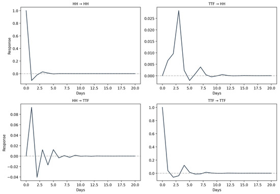
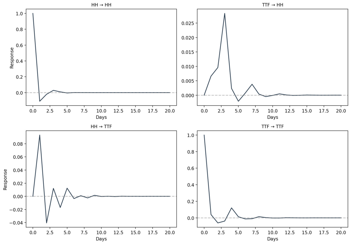
The premium on the TTF price, above the HH price, reflects shipping costs, regasification, and a tight LNG market in the Atlantic region. The VAR(4) impulse response functions (Figure 2) further reveal the unidirectional causation, where a positive return shock of one standard deviation on HH leads to positive returns in the TTF market within one trading day, and the response gradually decreases to zero after four to five trading days.

Figure 2. Impulse response functions from a VAR(4) on daily log returns, 2019–2024. Source: authors’ elaboration based on daily Henry Hub (NYMEX) and TTF (ICE) futures prices.

Conversely, a positive shock of returns to TTF has no discernible effect on HH returns at any horizon. This finding suggests that the European market reacts to information from the US benchmark, but the information does not pass back to the US. This result is consistent with a market structure in which the US acts as the marginal LNG supplier, the netback on which is the reference price at the bottom of the pricing ladder.

4.4. Conditional Volatility and Dynamic Correlation

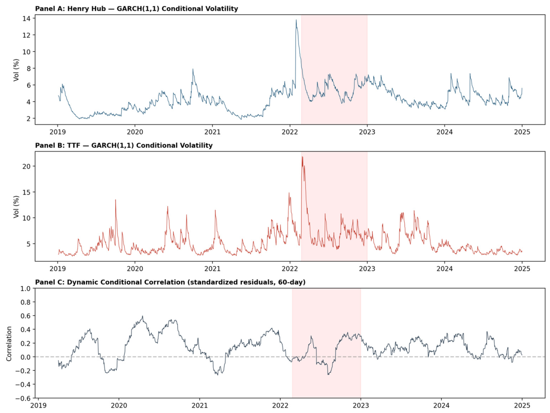
Table 5 shows the estimated parameters of the GARCH(1, 1) model. Both markets have near-unitary persistence in their conditional volatility (α + β = 0.997 for HH, 0.981 for TTF); that is, shocks to conditional variance dissipate quite gradually. The only notable asymmetry is in the ARCH coefficient.

Table 5. GARCH(1, 1) parameter estimates with Student-t innovations.

Parameter	HH	TTF
α (ARCH)	0.0762	0.163
β (GARCH)	0.9209	0.818
Persistence (α + β)	0.9971	0.981
ν (degrees of freedom)	6.76	6.45

Source: authors’ calculations based on daily Henry Hub (NYMEX) and TTF (ICE) futures prices.

The ARCH coefficient of TTF (α = 0.163) is more than twice that of HH (α = 0.076), which means that, for any given daily return, the European market reacts about twice as strongly as the American one. This difference is consistent with TTF being a thinner market, where a single large shipment diverted elsewhere or an interruption to a specific pipeline supply line can cause a sharp price spike. The estimated degrees-of-freedom parameter of the Student-t innovations is around 6.5 to 6.8 for both HH and TTF, so the returns of both markets have fat tails that call for a fat-tailed distribution of innovations rather than the normal distribution assumed in the baseline model.

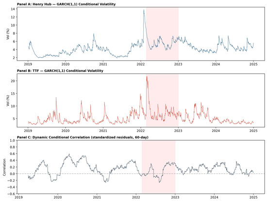
In Figure 3, Panel C, we plot the time-varying correlation of the standardized GARCH(1, 1) residuals for the two markets. We think of this correlation as a proxy for the dynamic conditional correlation (or market co-movement) that filters out the volatility clustering in the series. The correlation oscillates between roughly 0.4 and −0.4 over the sample, reaching its lowest levels during the first half of 2022 as the two series diverged, with HH falling on US mild weather and TTF rising on pipeline supply anxieties. By the end of the sample (late 2024), the correlation had returned to approximately 0.2 to 0.3. But this is still markedly below the correlation level in early 2019.

Figure 3. Conditional volatility and dynamic conditional correlation. Source: authors’ elaboration based on daily Henry Hub (NYMEX) and TTF (ICE) futures prices.

Table 5 thus offers further corroboration of the evidence from our cointegration analysis that HH and TTF were much more strongly linked, and, therefore, more tightly integrated, before 2022. The variance ratio σ²(TTF)/σ²(HH) offers a complementary perspective on the relative riskiness of the two markets across sub-periods.

TTF was 2.6 times more volatile than HH in 2019, converged to near parity during the pandemic (ratio 1.18 in 2020), then diverged again during 2021–2023 (ratios between 1.8 and 2.8). A striking reversal occurred in 2024, when the ratio dropped to 0.41, and TTF had become less volatile than HH. The likely explanation, we believe, is that the diversification of European gas sources has reduced price risk in the TTF market relative to the HH benchmark, where weather-driven variability of U.S. gas production in some sub-basins (such as the Permian) has introduced additional short-run noise.

4.5. Country Vulnerability Clusters

Table 6 shows import dependency and gas intensity for the fifteen most import-reliant countries in our sample. Germany (0.95) and Italy (0.95) are almost wholly reliant on imported gas, as domestic production of natural gas in the North Sea and the Po Valley has been declining. Poland (0.83) and the Netherlands (0.69) fall in the next group. Mexico, despite being an oil-producing country, has an import dependency of 0.64 (almost all imports are via pipeline from the United States) and the highest gas intensity (0.54 TWh per billion of GDP) among middle-income importers. It is thus especially vulnerable to disruption in pipeline trade. Hierarchical clustering (Ward’s method, four groups) identifies the following profiles of the 34 countries for which all data are available.

Table 6. Import dependency and gas intensity for selected countries (latest available year).

Country	Import Dependency	Gas Intensity	GDP/Capita (USD)	Cluster
Germany	0.953	0.17	56,104	Diverse importers
Italy	0.952	0.25	40,385	Diverse importers
Poland	0.829	0.23	25,104	Diverse importers
Netherlands	0.691	0.22	67,520	Diverse importers
Mexico	0.643	0.54	14,186	Self-sufficient/large
India	0.54	0.18	2695	Diverse importers
United Kingdom	0.503	0.17	53,246	Diverse importers
China	0.428	0.23	13,303	Self-sufficient/large
Thailand	0.408	0.92	7347	Diverse importers
United States	−0.145	0.11	85,373	Self-sufficient/large
Russia	−0.320	0.66	14,391	Self-sufficient/large
Qatar	−1.000	0.58	87,661	Wealthy exporters
Australia	−1.000	0.2	65,099	Wealthy exporters
Norway	−1.000	0.06	87,925	Wealthy exporters

Source: authors’ elaboration based on data from the Energy Institute [19] and the World Bank [20].

Group 1 contains wealthy, pure exporters (Australia, Israel, Norway, and Qatar), all with an import dependency of −1.0 and with moderate gas intensity. Group 2 consists of gas-intensive developing countries (Iran, Turkmenistan, Trinidad and Tobago, and Uzbekistan), with gas intensity ratios between 3 and 8 TWh per billion of GDP; their domestic subsidies and resource rents drive gas intensity orders of magnitude higher than the average for the OECD. Group 3 is a set of large countries that are broadly self-sufficient (the United States, China, Russia, Canada, Mexico, Saudi Arabia, and the UAE), with an import dependency close to zero and with a dominant role in the world’s overall gas consumption patterns. Group 4, containing nineteen countries, comprises a variety of import-reliant countries scattered along the middle of the dependency and intensity plane, including most of Europe, most of South and Southeast Asia, and countries in Latin America.

The purpose of this classification is to translate the benchmark-level fragmentation documented in Section 4.2, Section 4.3 and Section 4.4 into country-level exposure. Once arbitrage no longer ties HH and TTF together, a price shock at the European benchmark is no longer cushioned by transatlantic flows, so the welfare consequences of that shock fall unevenly across importers according to where they sit in the dependency and intensity plane. The clusters make this heterogeneity explicit. Group 4 is the segment most directly exposed to the transmission estimated in the panel regression because its members combine reliance on imported gas with the gas intensity that converts a price increase into a sizeable rise in the import bill. Within this group, the contrast between a highly dependent but low-intensity economy such as Poland and a moderately dependent but high-intensity economy such as Thailand or Mexico shows why import dependency alone understates exposure. The exporters in Group 1 and the large self-sufficient economies in Group 3, by contrast, are largely insulated from the same shock. Read together with the price results, the clustering, therefore, identifies the economies for which the loss of integration matters most, rather than serving as a stand-alone descriptive exercise. We test directly whether the price pass-through differs across these clusters in Section 4.10, where the diverse importers turn out to carry the largest elasticity.

4.6. Panel Regression Estimates

The fixed effects panel regression results are presented in Table 7. Only log GDP and import dependency variables enter the baseline Model 1. Neither is significant, and the within R² (0.007) is also very low. In this case, it is not surprising that neither of the variables is significant, as entity fixed effects soak up the variation between countries, leaving only a limited amount of variation in these two slowly moving structural variables to explain within country variations in the annual import values.

Table 7. Fixed-effects panel regression. Dependent variable: ln(import value, USD).

Variable	Model 1	Model 2	Model 3	Model 4
ln(GDP)	0.073	−2.284 *	−2.599	−1.147
	−1.27	−1.237	−1.658	−1.647
Import dependency	1.902	0.538	0.565	0.856
	−1.888	−2.41	−2.46	−3.073
ln(TTF)	—	0.520 **	0.499 **	—
		−0.206	−0.242
Russia dummy (≥2022)	—	—	0.129	—
			−0.382
Time FE	No	No	No	Yes
R2 (within)	0.007	0.064	0.065	−0.006
Observations	98	98	98	98
Countries	19	19	19	19

Source: authors’ estimates based on data from the Energy Institute [19], the World Bank [20], the UN Comtrade database [21], and TTF futures prices from ICE. Notes: Clustered standard errors in parentheses. * p < 0.10, ** p < 0.05.

In Model 2, we introduce the annual TTF average price (in logs), with a coefficient estimate of 0.520 (p = 0.014) within R² (0.064). We interpret the coefficient estimate of 0.520 to mean that for every 10 percent increase in the TTF price, we expect a 5.2 percent increase in the USD value of gas imports for all other variables kept constant. In Model 3, we augment the baseline with a post-2022 dummy Dₜ ≥ 2022:

$$\ln \left({\mathrm{I}\mathrm{m}\mathrm{p}\mathrm{o}\mathrm{r}\mathrm{t}\mathrm{s}}_{\mathrm{i}\mathrm{t}}\right)={\mathsf{\alpha }}_{\mathrm{i}}+{\mathsf{\beta }}_1\ln \left({\mathrm{G}\mathrm{D}\mathrm{P}}_{\mathrm{i}\mathrm{t}}\right)+{\mathsf{\beta }}_2{\mathrm{I}\mathrm{m}\mathrm{p}\mathrm{o}\mathrm{r}\mathrm{t}\mathrm{D}\mathrm{e}\mathrm{p}}_{\mathrm{i}\mathrm{t}}+{\mathsf{\beta }}_3\ln \left({\mathrm{T}\mathrm{T}\mathrm{F}}_{\mathrm{t}}\right)+{\mathsf{\beta }}_4{\mathrm{D}}_{\mathrm{t}\ge 2022}+{\mathsf{\epsilon }}_{\mathrm{i}\mathrm{t}}$$

(18)

The dummy coefficient is not significant (p = 0.74), suggesting that the main effect of the Russia crisis operated through the TTF price level rather than through any residual structural shift in import behavior. In Model 4, we substitute a fixed time effect for the TTF average price variable. Import dependency is still not significant, confirming that the low variation of this variable within a country over time (over a 6-year period) is not sufficient to identify a statistically significant effect on the import bill.

4.7. Robustness Checks

The baseline fixed-effects coefficient estimate of the TTF elasticity is subject to four tests of robustness (Table 8). Hausman test chi-squared of 6.856 (p = 0.077) is borderline between fixed and random-effects estimates, but random-effects estimate gives an import dependency coefficient that is both large (5.30) and highly significant (p < 0.001) and a TTF price coefficient that is insignificant (0.17, p = 0.38), which of course is consistent: random-effects estimates capture the cross-country variation between countries (where structural import dependency is the major determinant of import expenditure), while the fixed-effects estimator isolates the time series effect within a country (where year-to-year fluctuations in price matter), and so the two estimates are not really contradictory, just reporting information relevant to slightly different research questions about the nature of variation in our dataset.

Table 8. Model Robustness.

Specification	Price Coefficient	SE	p-Value	R2 (Within)
Baseline FE (Model 2)	0.52	0.206	0.014	0.064
Random effects	0.168	0.192	0.382	−0.012
FE with log(spread)	0.484	0.192	0.014	0.062
FE with log(TTF) + log(vol)	0.358	0.55	0.518	0.065
First differences	0.497	0.197	0.012	0.042

Source: authors’ estimates based on data from the Energy Institute [19], the World Bank [20], the UN Comtrade database [21], and TTF futures prices from ICE. Notes: Hausman test: χ² = 6.856, df = 3, p = 0.077. Wooldridge AR(1) test: ρ = −0.300, p = 0.010. All fixed-effects specifications use standard errors clustered at the entity level.

Likewise, the Wooldridge test gives rho = −0.30 (p = 0.010), indicating that first-order autocorrelation is indeed present in the FE residuals, suggesting that we were correct to use clustered error terms throughout; using transatlantic log spread (rather than TTF level) as independent variable produces an almost identical coefficient (0.48, p = 0.014), indicating that what we are picking up is really the European component of the price rather than some global price shock common to both benchmarks; using a first-differenced specification to address concerns about non-stationarity in levels:

$$\Delta \mathit{ln}\left({Imports}_{it}\right) = {\beta }_1\Delta \mathit{ln}\left({GDP}_{it}\right) + {\beta }_2\Delta {ImportDep}_{it} + {\beta }_3\Delta \mathit{ln}\left({TTF}_t\right) + \Delta {\epsilon }_{it}.$$

(19)

This yields a TTF elasticity of 0.50 (p = 0.012), practically indistinguishable from the baseline coefficient; the only estimator that produces an unstable result when introducing a measure of TTF volatility is the latter (due to collinearity between level and dispersion of price series with eightfold change in our sample), but otherwise the TTF price elasticity of approximately 0.5 appears to be robust to the choice of estimator or functional form or differentiation strategy, although, given the somewhat small panel dimensions, one should remain cautious in over-interpreting the estimated point coefficients.

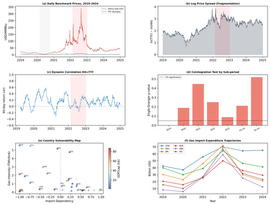
In contrast, Figure 4 encapsulates the takeaway of the paper. As we can see from Figure 4a–d, the pre-pandemic HH–TTF pricing mechanism has evolved towards a disconnected set of prices with the gap widening during the 2021–2022 European energy crisis, resulting in very high levels of the log spread during this period of time, as well as in the decline of the rolling return correlation towards 0 and even in negative values during this period. Both results suggest that HH and TTF were decoupled from the stable pricing system they used to be in prior to the pandemic. The results are confirmed by the cointegration results in sub-periods, whereby cointegration is only confirmed in 2019, while the null hypothesis of no cointegration cannot be rejected for the remaining periods, including for the first and second halves of 2024. Overall, all the figures show that the crisis in energy markets was more than just transitory, in line with the decoupling of the two gas markets.

Figure 4. The upper panel displays HH and TTF benchmark prices (a) and the respective log price spread (b). The bottom-left panel shows the 60-day rolling correlation of daily returns, and the bottom-right panel reports p-values of the Engle–Granger cointegration tests by sub-periods. The middle row presents each country’s exposure to natural gas prices using import dependency and gas intensity. Colors represent country-specific levels of GDP per capita. The right panel reports the development of gas import expenses in selected major importing economies. These charts suggest that the decline in transatlantic price integration from 2020 onwards corresponds to differential cross-country exposure to natural gas prices. Source: authors’ elaboration based on data from the Energy Institute [19], the World Bank [20], the UN Comtrade database [21], and daily Henry Hub (NYMEX) and TTF (ICE) futures prices.

Figure 4e,f build on this result, moving from benchmark behavior to macroeconomic exposure. The vulnerability map shows that import-dependence alone does not explain vulnerability: countries like Mexico or Thailand, for example, have moderate- or high-dependence on imported gas along with high gas-intensity, meaning they are relatively more vulnerable to a rise in the benchmark price. The wealthier exporter countries remain clustered at the lower end of the dependence distribution, and there are several European economies with high dependence but low gas intensity, compared to the countries with the highest exposure. The expenditure trajectory corroborates this evidence of heterogeneous impact: prices increased sharply and caused import expenditure to rise significantly for the largest importing economies in 2022, with only some of this impact reversing in 2023 and 2024. The qualitative results support the panel estimates shown previously, where a higher TTF price is also associated with higher import expenditure.

4.8. Regime-Switching Robustness

To put the structural interpretation on a firmer statistical footing, we estimate a two-regime Markov-switching AR(1) model on the daily log spread, allowing the intercept, the autoregressive coefficient, and the variance to switch between regimes. The estimates, reported in Table 9, separate a mean-reverting regime, with an autoregressive coefficient of 0.984, from a regime with a unit root, in which the coefficient equals 1.000, and the spread does not revert. We label the second regime as fragmented, in line with the operational definition of Section 3.3, because a unit root in the spread is exactly the condition under which any gap between the two benchmarks can persist without closing.

Table 9. Two-regime Markov-switching AR(1) estimates for the daily log spread, 2019–2024.

Parameter	Regime 0 (Integrated)	Regime 1 (Fragmented)
μ (intercept)	2.734	2.750
φ (AR coefficient)	0.984	1.000
σ (standard deviation)	0.094	0.039
Transition probability (stay)	0.949	0.964
Expected duration (trading days)	20	28

Source: authors’ own calculations based on the daily TTF–HH log spread New York Mercantile Exchange (NYMEX) and Intercontinental Exchange (ICE). Log-likelihood = 2106.97; AIC = −4197.94; BIC = −4155.39; N = 1509. The fragmented regime prevails in 59 percent of the sample days.

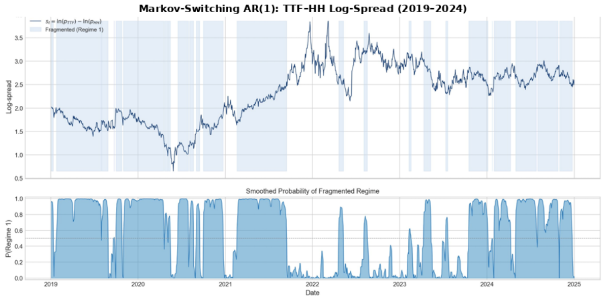
The fragmented regime is the more persistent of the two, with a probability of remaining in it of 0.964 and an expected duration of about 28 trading days, against 20 days for the mean-reverting regime, and it accounts for 59 percent of all sample days. Its smoothed probability, plotted in Figure 5, exceeds one-half for long stretches of the 2019 to 2021 period and becomes almost continuous from late 2023 through the end of 2024, which is consistent with the reduced-form finding that no sub-period after 2019 shows significant cointegration and that the spread carries a unit root over the full sample. One nuance deserves mention. During the acute phase of the 2022 crisis, the model assigns a higher probability to the mean-reverting regime, which also carries the larger variance, because the simultaneous spike in both benchmarks produces transient co-movement. In our framework, the fragmentation signal, therefore, comes from the persistence of the spread rather than from its volatility, and the regime-switching estimates reinforce, rather than replace, the sub-period cointegration evidence.

Figure 5. Markov-switching AR(1) regimes of the TTF–HH log spread, 2019–2024. The upper panel plots the daily log spread, with the shaded bands marking the days classified in the fragmented regime (Regime 1). The lower panel plots the smoothed probability of the fragmented regime, with the dashed line at 0.5. Source: authors’ calculations based on daily Henry Hub (NYMEX) and TTF (ICE) futures prices.

4.9. Endogeneity and Identification Checks

A remaining concern is that the TTF price and the import bill could be jointly determined, or that the largest importers might influence the European benchmark. We address these concerns with the additional checks reported in Table 10, estimated on the panel of net-importing countries. Excluding the two largest importers that are most likely to affect the benchmark, Germany and China, leaves the elasticity virtually unchanged, at 0.426 against a baseline of 0.432, which is difficult to reconcile with reverse causation running from a single importer to the benchmark. Excluding two further large importers, Italy and the United Kingdom, lowers the point estimate to 0.325, but the sample then falls to eleven countries, and the estimate loses precision. Replacing the contemporaneous price with its one-year lag, which breaks the within-year simultaneity, yields a smaller but still positive and marginally significant coefficient of 0.171, consistent with a pass-through that is concentrated in the year of the price change.

Table 10. Endogeneity and identification checks. Dependent variable: ln(import value, USD).

Specification	Price Coef.	SE	p-Value	R2 (Within)	N
Baseline FE (importer panel)	0.432	0.199	0.033	0.081	89
Excluding DEU, CHN	0.426	0.233	0.073	0.076	77
Excluding DEU, CHN, ITA, GBR	0.325	0.277	0.246	0.062	65
Lagged ln(TTF), t − 1	0.171	0.091	0.066	0.050	74

Source: authors’ estimates based on data from the Energy Institute [19], the World Bank [20], the UN Comtrade database [21], and TTF futures prices from ICE. Standard errors clustered at the country level. A two-stage least squares specification instrumenting the benchmark with its one-year lag is not viable in this panel: with six annual price observations, the first-stage F-statistic is 0.02, far below conventional thresholds, so the instrumented estimate is uninformative.

We also attempted a formal instrumental-variables strategy, instrumenting the annual TTF average with its one-year lag, but with only six annual price observations, the instrument is extremely weak, with a first-stage F-statistic of 0.02, and the resulting estimate is uninformative. This confirms the caution stated in Section 3.3: a credible instrument for the benchmark would need a longer annual series than the present sample provides. Taken together, the subsample and lag checks support reading the elasticity as a robust conditional pass-through that is consistent with a causal channel, while the failure of the instrumented specification marks the limit of what can be identified with these data.

4.10. Cross-Cluster Heterogeneity in the Price Pass-Through

Section 4.5 argued that the loss of integration matters most for the cluster of diverse importers. We test this directly by interacting the annual TTF price with the vulnerability clusters of Table 6. Table 11 reports two specifications. Model 1 assigns a separate price elasticity to each cluster that contains at least two of the countries with complete trade data; the wealthy-exporters cluster, represented by a single country in the panel, is absorbed into the fixed effects. Model 2 is a more parsimonious contrast that keeps a common price term and adds a single interaction for the diverse importers, and we treat it as the cleaner anchor because it avoids the issue noted below.

Table 11. Cross-cluster heterogeneity in the TTF price elasticity. Dependent variable: ln(import value, USD).

Variable	Model 1	Model 2
ln(GDP)	0.642 *** (0.016)	–1.551 (1.362)
Import dependency	3.638 *** (0.888)	3.642 *** (0.948)
ln(TTF)	—	0.176 (0.278)
ln(TTF) × diverse importers	0.691 *** (0.195)	0.598 * (0.322)
ln(TTF) × self-sufficient/large	0.261 *** (0.046)	—
ln(TTF) × other	0.028 (0.270)	—
R2 (within)	0.091	0.109
Observations	89	89
Countries	15	15

Source: authors’ estimates based on data from the Energy Institute [19], the World Bank [20], the UN Comtrade database [21], and TTF futures prices from ICE. Clustered standard errors in parentheses. * p < 0.10, *** p < 0.01. Clusters follow the classification in Table 6, and the wealthy-exporters cluster (one country in the panel) is absorbed by the fixed effects. A Wald test of equality of the three cluster elasticities in Model 1 gives F = 2.83 (p = 0.066). In Model 1, the three interaction terms exhaust the variation in ln(TTF), so the ln(GDP) coefficient is identified differently than in the other panel specifications and is not comparable to them; Model 2 retains a common ln(TTF) term and is the preferred specification.

The pass-through is far from uniform. In Model 1, the diverse importers, the European and Asian economies that combine reliance on imported gas with non-trivial gas intensity (Germany, Italy, the United Kingdom, the Netherlands, and Thailand), show the largest elasticity, 0.691, significant at the one percent level. The large, broadly self-sufficient economies present in the panel (China and Mexico) show a smaller but still significant elasticity of 0.261, and the remaining countries, which are mostly exporters or balanced producers, show an elasticity close to zero. A Wald test rejects the equality of the three elasticities at the ten percent level (F = 2.83, p = 0.066). Because the three interactions in Model 1 fully decompose the price term, we read the size of the cluster elasticities from this model but rely on Model 2 for the headline contrast and for the other coefficients. Model 2 keeps a common price term and adds a single interaction for the diverse importers, which is positive and marginally significant (0.598, p = 0.068); the implied elasticity for the diverse importers is about 0.77, against roughly 0.18 for the rest of the panel.

This heterogeneity is the country-level counterpart of the benchmark-level fragmentation. The economies that the clustering identifies as most exposed are precisely those whose import bills respond most strongly to the European benchmark, which is the welfare channel through which a fragmented and volatile market reaches importing economies. The result should be read with the same caution as the rest of the panel evidence, since the test rests on fifteen countries and the significance is marginal, but the ordering of the elasticities is economically coherent and stable across the two specifications.

5. Discussion

The main result of this paper is that the global natural gas market was fragmented in 2020 and had not reconnected by the end of 2024. Cointegration between HH and TTF, which was present in 2019 when LNG arbitrage held the spread close to a stable long-run level, broke down with the onset of the pandemic and weakened further during the Russia crisis. By the end of the sample, the spread is non-stationary, the rolling correlation of daily returns is almost never above 0.3, and no sub-period since 2019 exhibits significant cointegration. Taken together, and in line with the operational definition set out in Section 3, these results indicate not a transient disruption but a market that has settled into a new regime.

The asymmetry in causality, from HH to TTF, but not in reverse, has a very straightforward economic justification. The U.S. became the largest LNG exporter in the world in 2023, and HH price plus liquefaction plus shipping costs set a price floor below which U.S. LNG cargoes are not sold in Europe.

European prices can and do exceed this threshold by a large margin in times of very high European demand or when pipeline supply collapses, but they cannot fall much below the threshold without eliminating the flow of arbitrage. The U.S. market, on the other hand, is insulated from what’s going on in Europe by virtue of its own production, which amounts to more than 10,000 TWh per year, and because LNG exports still represent only about 15 percent of total US output. We think this asymmetry will persist until such time as U.S. LNG exports saturate, or until European demand weakens to the point where trans-Atlantic LNG no longer provides the marginal supply.

The GARCH estimates provide a volatility counterpart to the price fragmentation picture. The larger ARCH coefficient in TTF (0.163, compared to 0.076 in HH) means that a given shock, in the form of a plant breakdown, a bout of cold weather, or perhaps an unexpected headline in geopolitics, moves the European market roughly twice as far as it would move the American one. This is bad news for European importers who take their TTF-indexed contracts into their budgets. Near-integrated persistence (α + β ≈ 1) in both markets means that, once volatility has become elevated, it stays elevated for some time. As one may expect, volatility jumped to particularly high levels during 2022, when conditional volatility in TTF exceeded 20 per cent on some days, highlighting the tail risks that the importing countries face.

6. Conclusions

The results of this paper show that integration of the global natural gas market experienced a structural break, with measurable consequences for energy-importing countries. The central finding is that the HH and TTF log-price series moved from a cointegrated relationship in 2019 to a pattern of non-convergence from 2020 onward. The Engle and Granger test rejects the null of no cointegration only in 2019 (statistic of −4.286, p = 0.003) and fails to reject it in every later sub-period, including both halves of 2024, while the transatlantic spread carries a unit root over the full sample. Three conclusions follow, each tied to a specific piece of the evidence.

(i)

The global gas market is no longer a single market when measured by its two leading benchmarks. The non-stationary spread, together with a rolling return correlation that falls from about 0.4 toward zero and at times to −0.3, indicates that regional factors such as infrastructure limits and perceived geopolitical risk have overwhelmed the arbitrage that LNG trade would otherwise provide.

(ii)

Price discovery across the two leading markets is asymmetric. The Granger causality tests and the VAR impulse responses show that Henry Hub leads TTF (F = 9.69, p = 0.002 at one lag), while shocks to TTF have no measurable effect on Henry Hub, which is consistent with the United States acting as the marginal LNG supplier that sets the price floor for transatlantic cargoes. A practical implication is that European prices cannot be capped through LNG supply alone, so demand-side and storage measures are the more reliable instruments for influencing European natural gas prices.

(iii)

The country-specific degree of exposure to gas price shocks depends jointly on import dependency and gas intensity, not on either alone. The fixed-effects estimate places the TTF price elasticity of the import bill near 0.5 and remains stable across the first-differenced and spread-based specifications, so an economy that is only moderately dependent on imports but highly gas-intensive, such as Thailand or Mexico, can face welfare losses comparable to, or larger than, those of a highly dependent but less gas-intensive European economy.

These findings are reinforced by three additional exercises. A two-regime Markov-switching model identifies a persistent, non-mean-reverting regime that dominates the sample and becomes almost continuous through 2024 (Section 4.8); a set of identification checks leaves the price elasticity essentially unchanged when the largest importers are removed (Section 4.9); and a test of cluster heterogeneity confirms that the diverse importers carry the largest pass-through, with an elasticity near 0.77 against about 0.18 for the rest of the panel (Section 4.10). Two avenues remain open. A credible instrument for the benchmark price, drawing on weather or storage shocks measured over a longer annual series, would move the pass-through estimate closer to a point-identified causal effect, since the lagged-price instrument is too weak in the present six-year panel. Finally, replacing the estimated trade flows with bilateral data, for example, from the BACI-CEPII database, would allow gas trade networks to be built on observed rather than inferred flows.

Another research question that will have to be addressed in a more structural model is the relationship between the flexibility of LNG, destination versus destination-fixed contracts, and the transmission of inter-regional gas prices. Such work would likely benefit from detailed information on individual contracts, or even individual shipments, but such information is clearly beyond the scope of the data available to the present study.

This paper contributes to the existing literature by arguing that the fragmented nature of natural gas prices can act as an important channel through which the economy is exposed to foreign shocks. The paper provides evidence to support this argument by synthesizing a price transmission framework, a volatility model, and an indicator of country-specific vulnerability. The results support the proposition that energy security depends jointly on market structure, dependence on imported gas, and, finally, the share of natural gas in production technology. These findings may prove helpful in future empirical work as well as policy-oriented research that seeks to reduce economies’ vulnerability to the emerging segmented and volatile international gas markets.

References

- Neumann, A. Linking Natural Gas Markets—Is LNG Doing its Job? Energy J. 2009, 30, 187–199. [Google Scholar] [CrossRef] [Scilit]
- Li, R.; Joyeux, R.; Ripple, R.D. International Natural Gas Market Integration. Energy J. 2014, 35, 159–180. [Google Scholar] [CrossRef] [Scilit]
- Shen, Y.; Shi, X.; Variam, H.M.P. Risk Transmission Mechanism between Energy Markets: A VAR for VaR Approach. Energy Econ. 2018, 75, 377–388. [Google Scholar] [CrossRef] [Scilit]
- Nick, S.; Thoenes, S. What Drives Natural Gas Prices?—A Structural VAR Approach. Energy Econ. 2014, 45, 517–527. [Google Scholar] [CrossRef] [Scilit]
- Cherp, A.; Jewell, J. The Concept of Energy Security: Beyond the Four As. Energy Policy 2014, 75, 415–421. [Google Scholar] [CrossRef] [Scilit]
- Sovacool, B.K.; Mukherjee, I. Conceptualizing and Measuring Energy Security: A Synthesized Approach. Energy 2011, 36, 5343–5355. [Google Scholar] [CrossRef] [Scilit]
- Barrera-Rivera, R.R.; Valencia-Herrera, H. Dynamic Hedging of Prices of Natural Gas in Mexico. Rev. Mex. Econ. Finanz. 2020, 15, 353–374. [Google Scholar] [CrossRef] [Scilit]
- Mendoza-Rivera, R.J.; Venegas-Martínez, F. Impacto de la Pandemia COVID-19 en los Precios de la Gasolina y el Gas Natural en las Principales Economías de Latinoamérica. Rev. Mex. Econ. Finanz. 2021, 16, e654. [Google Scholar] [CrossRef] [Scilit]
- Pérez-Guzmán, K.; Téllez-León, I.E.; Kharrazi, A.; Fath, B.; Venegas-Martínez, F. What Makes Input–Output Tables of Trade of Raw Material Goods Peculiar Networks? The World and Mexican Cases. Rev. Mex. Econ. Finanz. 2018, 13, 483–505. [Google Scholar] [CrossRef] [Scilit]
- Peng, P.; Lu, F.; Cheng, S.; Yang, Y. Mapping the Global Liquefied Natural Gas Trade Network: A Perspective of Maritime Transportation. J. Clean. Prod. 2021, 283, 124640. [Google Scholar] [CrossRef] [Scilit]
- Xiao, Y.; Chen, Y.; Liu, X.; Yan, Z.; Cheng, L.; Li, M. Structural Analysis and Robustness Assessment of Global LNG Transport Network from 2013 to 2023. Ocean. Coast. Manag. 2025, 263, 107600. [Google Scholar] [CrossRef] [Scilit]
- Baba, A.; Creti, A.; Massol, O. What Can Be Learned from the Free Destination Option in the LNG Imbroglio? Energy Econ. 2020, 89, 104764. [Google Scholar] [CrossRef] [Scilit]
- Chiappini, R.; Jégourel, Y.; Raymond, P. Towards a Worldwide Integrated Market? New Evidence on the Dynamics of U.S., European and Asian Natural Gas Prices. Energy Econ. 2019, 81, 545–565. [Google Scholar] [CrossRef] [Scilit]
- Farag, M.; Jeddi, S.; Kopp, J.H. Global Natural Gas Market Integration: The Role of LNG Trade and Infrastructure Constraints. World Econ. 2025, 48, 1405–1417. [Google Scholar] [CrossRef] [Scilit]
- Emiliozzi, S.; Ferriani, F.; Gazzani, A. The European Energy Crisis and the Consequences for the Global Natural Gas Market. Energy J. 2025, 46, 119–145. [Google Scholar] [CrossRef] [Scilit]
- Asche, F.; Oglend, A.; Osmundsen, P. Modeling UK Natural Gas Prices when Gas Prices Periodically Decouple from the Oil Price. Energy J. 2017, 38, 131–148. [Google Scholar] [CrossRef] [Scilit]
- Halser, C.; Paraschiv, F.; Russo, M. Oil–Gas Price Relationships on Three Continents: Disruptions and Equilibria. J. Commod. Mark. 2023, 31, 100347. [Google Scholar] [CrossRef] [Scilit]
- Loureiro, J.R.; Inchauspe, J.; Aguilera, R.F. World Regional Natural Gas Prices: Convergence, Divergence or What? New Evidence. J. Commod. Mark. 2023, 32, 100368. [Google Scholar] [CrossRef] [Scilit]
- Energy Institute. Statistical Review of World Energy, 73rd ed.; Energy Institute: London, UK, 2024. [Google Scholar]
- World Bank. World Development Indicators. Available online: https://data.worldbank.org (accessed on 17 April 2026).
- United Nations. UN Comtrade Database. Available online: https://comtradeplus.un.org (accessed on 17 April 2026).
Disclaimer/Publisher’s Note: The statements, opinions and data contained in all publications are solely those of the individual author(s) and contributor(s) and not of MDPI and/or the editor(s). MDPI and/or the editor(s) disclaim responsibility for any injury to people or property resulting from any ideas, methods, instructions or products referred to in the content. |
© 2026 by the authors. Licensee MDPI, Basel, Switzerland. This article is an open access article distributed under the terms and conditions of the Creative Commons Attribution (CC BY) license.