


Abstract
Photovoltaic fault detection and maximum power point tracking are commonly treated as separate functions, although both depend on irradiance, temperature, electrical state and data quality. This study develops a physics-guided framework that links measured fault detection to diagnosis-dependent supervisory MPPT while keeping measured diagnostic evidence separate from control-software evidence. The Lahore dataset contains 217,196 timestamped records and 19,452 unique physical fault-event groups from one grid-tied inverter with two monitored MPPT channels. Fault events are separated chronologically at the physical-event level, and calibration and threshold selection use Training + Validation data only. The HGB detector using the complete operational representation achieved 99.46% Test accuracy and macro-F1, with MCC 0.9892 and AUROC 0.9998. Permutation importance showed strong dependence on sequence-availability descriptors; a residual-free and quality-free design using only logged electrical, environmental and grid channels achieved 88.79% Test accuracy. In a separate static P–V software benchmark, the diagnosis-dependent supervisory P&O controller achieved 99.96% mean tracking efficiency and 0.193 V mean simulated voltage-reference oscillation on a restricted 240-event subset. The control experiment contains no converter dynamics or physical time base and the measured diagnosis evidence is limited to one PV installation. External plant validation and converter-level testing are therefore required before broader operational transfer.
1. Introduction
Photovoltaic (PV) plants operate under changing irradiance, module temperature, grid conditions, converter states and sensor quality. These variations can obscure electrical faults because normal weather-driven changes and abnormal equipment behavior can produce similar voltage, current and power responses. A recent review of PV degradation mechanisms emphasizes that early electrical detection is important because apparently mild degradation can propagate into energy loss or safety risk [1].
Data-driven methods are increasingly used for photovoltaic monitoring. A systematic review found that machine-learning and deep-learning methods can extract nonlinear fault signatures from large monitoring datasets, but their reported performance depends strongly on data quality, validation design and the representativeness of fault labels [2]. A broader review of PV fault detection similarly identified the separation between model-based residual methods, electrical-feature classifiers and image or thermal approaches as a persistent methodological challenge [3].
A bibliometric analysis of more than 620 publications further showed the rapid growth of AI-based PV fault diagnosis and the need to distinguish algorithmic novelty from sound data and validation practice [4].
Measured-data validation is particularly important. Ensemble methods can perform well for PV diagnosis, but performance obtained from randomly mixed or synthetically perturbed samples does not necessarily demonstrate generalization to independent operating events [5]. Electrical classifiers should therefore be trained and tested on disjoint fault events, with confirmation and maintenance records excluded from the predictor set. Event grouping is also necessary when a fault interval and its pre-fault baseline originate from the same physical episode [6].
PV fault evidence is naturally temporal. Convolutional and recurrent networks have been used to combine local electrical patterns with longer sequence behavior [7]. Lightweight deep models have also been proposed for edge-oriented diagnosis, although their computational cost, calibration and response to sensor errors must be reported before real-time use is inferred [8]. Graph neural networks offer a further direction by encoding electrical and topological relations under sparse measurements and volatile PV generation [9]. At the wider energy-system level, adjustable-conservativeness strategies show how data-driven predictions can be translated into risk-aware operational decisions rather than being treated as isolated forecasts [10].
Maximum power point tracking (MPPT) and fault detection are often studied separately even though both depend on the same PV operating state. Conventional perturb-and-observe (P&O) and incremental-conductance (INC) controllers remain practical benchmarks, while intelligent MPPT methods trade additional complexity for faster adaptation under nonlinear and partially shaded characteristics [11]. Experimental work has demonstrated that learned MPPT can improve transient tracking, but laboratory validation and explicit conventional baselines remain essential [12]. Temporal irradiance forecasting has likewise been used to anticipate the maximum-power voltage under changing conditions [13].
Partial shading makes the connection between diagnosis and control especially clear. Bypass-diode activation creates steps in the current–voltage (I–V) characteristic and multiple local maxima in the power–voltage (P–V) characteristic [14]. Bypass-diode faults can themselves be detected from electrical behavior, but shading and diode abnormalities can overlap in their observed signatures [15]. A diagnosis-control study should therefore represent multiple power maxima, compare conventional trackers and show how the diagnostic output changes the control trajectory. In this study, multi-maximum behavior is examined separately in parameterized shading and bypass-diode cases; it is not represented in the restricted 240-event event-specific control subset.
Few studies combine operationally logged plant fault events, chronological event-group separation, physically interpretable electrical residuals, group-preserving probability calibration and an explicit diagnosis-to-control pathway. The framework therefore separates two evidence levels. The measured branch evaluates fault detection on independent chronological event groups from one PV installation. The control branch maps held-out measured events to parameterized static P–V scenarios and evaluates how diagnostic state, measured electrical severity and data quality change supervisory MPPT actions. This separation prevents software control results from being interpreted as closed-loop field validation.
The principal contributions are as follows:
- 1.
- A measured-data diagnosis protocol uses 19,452 logged fault-event groups indexed by Physical_Event_ID, matched pre-fault baselines, explicit logged-onset alignment and chronological event-group partitioning. The retained fault categories are taken directly from the logged Event_Label; confirmation, suspected-fault, alarm, maintenance, repair and technician fields remain audit-only and are excluded from model predictors. The supplied export does not identify whether Event_Label originated from inverter logic, operator annotation, or a separate inspection process, so these categories are treated as supplied operational labels rather than independently re-verified hardware failures.
- 2.
- The operational HGB combines an outlier-resistant healthy-power expectation with a validation-selected 228-feature representation containing electrical, environmental, grid, residual, transition and data-availability descriptors. Because coverage features can encode properties of the event export, their importance is reported explicitly and a raw physical-channel, residual-free and quality-free ablation is provided as a conservative physical-signal cross-check. Final probabilities use five-fold group-preserving out-of-fold calibration without test-data reuse.
- 3.
- Predictive evidence includes event-group bootstrap analysis, paired testing, feature and branch ablation, causal detection-delay analysis, environmentally matched testing, class-specific selective rejection, sensor-noise and missing-data stress, irradiance-bias cross-checking and a dedicated arc-versus-insulation secondary analysis.
- 4.
- A three-substring single-diode model with bypass diodes maps measured fault events to fault-specific static proxies whose severity is derived from pre-fault-to-active electrical deficits. A diagnosis-dependent supervisor changes voltage step, scan interval, ramp limit, data-quality hold and a protective delivered-power scaling proxy. Fault-severity, supervisory-setting and PV-parameter sensitivity are reported separately from the event-specific comparison with P&O and INC.
2. Related Work and Research Position
2.1. Electrical and Data-Driven PV Fault Diagnosis
Electrical monitoring is attractive because voltage, current and power are normally available at the inverter or MPPT channel. Recent comparative work has examined supervised classifiers for PV array failures and has shown that no single classifier is uniformly best across operating and fault conditions [16]. This motivates a model whose nonlinear capacity is balanced by explicit validation, calibration and computational reporting.
I–V characteristics provide richer physical information than a single maximum-power operating point. Liu et al. used variable predictive models and I–V curves to improve PV array fault diagnosis [17]. Yang et al. used converted I–V characteristics to study multiple partial-shading conditions and their severity [18]. Lin et al. combined curve representations with environmental inputs and reported field-oriented fault identification, demonstrating the value of physically meaningful multi-input designs [19].
Environmental correction must be handled cautiously. IEC 60891:2021 defines procedures for translating measured I–V curves across irradiance and temperature conditions [20]. Li et al. showed that correction accuracy depends on the fault mechanism and that partial shading and bypass-diode conditions can be particularly difficult [21]. For this reason, the primary measured-data task in this study uses monitored operating sequences and a healthy environmental baseline; simulated I–V/P–V curves are used only to examine control behavior and secondary fault morphology.
Temporal models can identify persistence and transients that are invisible in a single sample. Amiri et al. combined convolutional and bidirectional gated recurrent units to exploit local and sequential information [7]. The present study retains a temporal convolutional model as a comparator. HGB was retained empirically because it produced the strongest Validation macro-F1 for the selected operational representation while requiring substantially lower host-software inference time than the secondary safety gated fusion.
2.2. Physics-Based PV Modeling and Partial Shading
PV modeling under partial shading requires more than a single-knee empirical curve. Bypass-diode state, series resistance, shunt resistance, substring irradiance and cell temperature determine whether steps or multiple local maxima appear. Experimental analysis of bypass-diode behavior under nonuniform irradiance confirms that diode activation changes both electrical characteristics and temperature distribution [14]. Recent system studies also show that bypass-diode configuration and inverter efficiency affect the energy consequences of shading [22].
The simulation benchmark uses a three-substring single-diode model with bypass diodes to reproduce stepped P–V characteristics and multiple local maxima for the control comparison and secondary morphology analysis.
2.3. MPPT and Diagnosis-to-Control Coupling
Recent MPPT reviews organize methods into conventional, artificial-intelligence and metaheuristic families and emphasize tracking efficiency, convergence, ripple, sensing requirements and implementation complexity [23]. Another recent review identifies controller validation under partial shading and changing operating conditions as a continuing challenge [24]. These criteria motivate direct comparison with P&O and INC rather than comparison only among learned controllers.
The main control contribution is the direct translation of diagnostic states into supervisory MPPT actions. An accepted abnormal state triggers a fault-adaptive scan and protective delivered-power scaling proxy; an uncertain state triggers a conservative scan; and a healthy state retains ordinary tracking. This closes the diagnosis-to-control path while keeping safety-induced power reduction distinct from tracking error.
3. Materials and Methods
3.1. Architecture and Evidence Levels
The framework contains two evidence-separated branches: measured-data fault detection and parameterized supervisory MPPT simulation. Figure 1 presents the measured-data path from plant channels to calibrated HGB states. Figure 2 presents the separate parameterized PV and supervisory MPPT simulation. This separation distinguishes measured diagnostic validation from simulation-based control evaluation.
Figure 1.
Measured-data architecture of the event-grouped HGB detector.
Figure 2.
Simulation architecture of the diagnosis-dependent MPPT supervisor.
The evidence hierarchy follows the split in Figure 1 and Figure 2. Measured healthy-versus-fault detection is the primary diagnostic evidence. Arc-versus-insulation classification is included as a secondary subtype analysis. The nine-class morphology and maximum power point tracking experiments provide a separate simulation-based assessment of curve behavior and supervisory control. The measured-data branch evaluates fault detection, while supervisory control is evaluated in the separate simulation branch.
The analysis distinguishes the plant dataset, the measured diagnosis set and the parameterized simulation set. The Lahore plant dataset contains 217,196 logged records and 19,452 logged fault-event groups indexed by Physical_Event_ID. In the retained audit, each Physical_Event_ID maps to exactly one labeled fault-event identifier. The measured diagnosis set contains 38,904 matched sequences, comprising one abnormal sequence and one pre-fault healthy sequence for each fault event. The chronological Test partition contains 4812 abnormal sequences and 4812 matched pre-fault baselines. The parameterized simulation denotes software-generated I–V/P–V curves, the separate nine-class morphology experiment and a deterministic 240-event MPPT benchmark sampled from held-out abnormal Test events. The capped MPPT subset contains only InsulationFault, ArcFault and LooseConnector events and is therefore treated as a restricted control stress test rather than a balanced six-class benchmark.
3.2. PV Plant, Hardware and Data Acquisition
The plant dataset was collected from a grid-connected PV installation in Lahore, Pakistan, from 14 January 2026 at 13:46:35 to 12 July 2026 at 23:41:21. The exact site coordinates are withheld because the records belong to an operating plant. The exported records identify one MAXPower grid-tied inverter, firmware version 2.1.0, with two monitored MPPT channels. MPPT 1 is mapped to the logged string identifier String 1A and MPPT 2 is mapped to String 2A. The installed equipment is shown in Figure 3 and Table 1 reports the plant information supported by the supplied records.
Figure 3.
MAXPower inverter, protection enclosure and associated battery-storage hardware at the monitored Lahore PV plant.
Table 1.
PV plant and data-acquisition information available in the plant export.
The plant monitoring system supplied the eight logged channels used by the detector. Photovoltaic power was obtained from the plant monitoring export and treated as a logged operating channel. Short within-event gaps of at most two samples were linearly interpolated within each event, while the original missing fraction was retained as a data-quality feature. No interpolation was performed across separate events. The final notebook does not construct a separate diagnosis tensor for each MPPT channel. Records from both monitored MPPT channels are pooled within each Associated_Event_ID; after sorting by timestamp, duplicate timestamps are collapsed to the first retained record before interpolation to the nominal sequence grid. The healthy-power regression and voltage/current normalization are therefore fitted jointly across both MPPT channels using Training-period healthy records rather than as channel-specific models. The MPPT_ID stored in the sequence metadata is the first retained channel identifier for that event and should not be interpreted as evidence that the complete sequence is channel-isolated.
3.3. Dataset, Event Labels and Leakage Control
The updated plant dataset contains 217,196 timestamped records and 19,452 logged fault-event groups. The dataset audit reports 19,452 unique Physical_Event_ID groups, equal to the associated fault-event count, so no retained physical-event identifier contains multiple associated fault identifiers. The event inventory comprises 7315 insulation-fault, 5211 arc-fault, 2104 hotspot, 1765 soiling, 1529 loose-connector and 1528 partial-shading groups. The audit identifies one plant, one inverter, two MPPT channels, 32,167 inspected healthy rows and no duplicate event–timestamp–MPPT records. Label-normalization auditing shows that all retained active-fault rows used Event_Label directly; the Confirmed_Fault and Suspected_Fault fallback paths contributed zero retained primary fault labels. The supplied workbook does not contain a provenance field establishing whether Event_Label itself was generated by inverter logic, operator annotation, engineering inspection, or another process. Accordingly, the 19,452 groups are treated as logged operational fault-event groups and not as 19,452 independently re-verified hardware failures. Table 2 reports their counts.
Table 2.
Logged fault-event groups indexed by Physical_Event_ID in the plant dataset.
The raw physical input matrix is restricted to an eight-channel allow-list: PV voltage, PV current, PV power, irradiance, module temperature, ambient temperature, grid voltage and grid frequency. Derived channels are then formed from the healthy-power expectation, voltage/current normalization and sequence-availability indicators. Alarm code, alarm-active state, confirmed-fault fields, confirmation method and status, technician or confirmation identifiers, maintenance action and outcome, post-repair verification, insulation-resistance measurements, hotspot temperature difference, shading-area estimates, soiling-level estimates, suspected-fault fields and fault-affected flags are retained only for auditing and are excluded from predictors. The full operational model therefore uses the eight logged physical channels plus derived residual/normalization and data-availability descriptors; these derived families are reported separately in the ablation and importance analyses. The origin and analytical role of these quantities are summarized in Table 3.
Table 3.
Origin and analytical role of the quantities used in the study.
Every fault event supplies two diagnosis samples: an abnormal sequence and its matched pre-fault healthy sequence. Fault onset is defined as the earliest timestamp whose logged Event_Phase equals Active-Fault. This is the recorded label onset and is not an independently measured physical inception time. The abnormal sequence is aligned to that onset on a nominal 5 min grid using six pre-fault offsets at , , , , and min and four active-fault offsets at 0, 5, 10 and 15 min. The matched healthy sequence contains ten pre-fault-only offsets at , , , , , , , , and min; no active-fault measurement is permitted to enter that matched baseline. Target points outside the available source interval are edge-held only to preserve tensor dimensions and are explicitly marked unavailable. At each original record, DataQualityFlag=1 when the logged Data_Quality_Flag equals “Good” (case-insensitive) and 0 otherwise. ObservedFraction=1-RawMissingFraction, where RawMissingFraction is the fraction of the eight allow-listed raw channels missing before interpolation. Both quantities are interpolated to the nominal grid with the other sequence channels and ObservedFraction is additionally forced to 0 for target times outside the observed source interval. Neither variable uses Event_Label, alarm status, confirmation, maintenance, repair, or technician fields. However, because the healthy and abnormal classes use different relative time windows by construction, availability descriptors can encode event-export and sequence-construction structure. Their contribution is therefore reported explicitly and is not interpreted as purely electrical fault evidence. Because the raw event records contain timestamp jitter and incomplete grid coverage, the 5 min values denote nominal alignment points rather than an assertion of exact uniform raw sampling.
The chronological split is defined at the physical-event-group level using the logged physical-event identifier when available. Training events end on 30 April 2026, validation events cover May 2026 and Test events begin on 1 June 2026. The dataset audit found the same 19,452 unique associated and physical fault-event groups and both members of each matched abnormal/healthy pair remain in the same partition. Table 4 reports the sequence counts. The resulting diagnosis set contains 22,752 Training sequences, 6528 Validation sequences and 9624 Test sequences.
Table 4.
Chronological event-group composition of the measured diagnosis dataset. Negative-class counts are matched pre-fault baselines.
Figure 4 and Figure 5 show the measured electrical and environmental channels over their complete time axes. Separate three-row layouts preserve the physical units and show the operating range represented by the event groups.
Figure 4.
Measured PV voltage, current and power over the complete plant dataset time axis.
Figure 5.
Measured irradiance, module temperature and ambient temperature over the complete Lahore plant dataset time axis.
3.4. Healthy-Power Expectation and Physically Interpretable Residuals
An environmental baseline is fitted only to inspected healthy records in the training period. Let denote normalized irradiance and let denote module-temperature deviation from 25 °C. The expected healthy power is:
where the coefficient vector minimizes the Huber objective
Equation (1) adjusts the expected power for irradiance and module temperature, while Equation (2) limits the influence of large training residuals without treating the regression as a first-principles PV model. The final implementation uses scikit-learn 1.6.1 HuberRegressor(epsilon=1.5, max_iter=1000). The epsilon value is the Huber transition in units of the estimator’s fitted robust residual scale, rather than a fixed 1.5 W threshold. With the design vector and the estimator’s fitted intercept combined into the constant term, the final run gives the effective coefficients , , and for Equation (1). The model and voltage/current normalization are fitted jointly across both MPPT channels using inspected healthy Training-period records only. The measured-to-expected ratio and normalized residual are
Equation (3) expresses the electrical response relative to the operating-condition-adjusted expectation. Voltage and current are also normalized by their healthy-training medians. The implemented denominator floor is 1 W; consequently, very low predicted power can produce large ratio or residual magnitudes, as visible in Figure 6. These residuals are therefore not interpreted as standalone physical evidence. The raw electrical+environment+grid ablation in Section 4 provides a residual-free and quality-free cross-check of classification using only logged physical channels. Figure 6 relates the environmental input, expected power, measured power, voltage, current and residual quantities. The scatter representation is retained because these panels compare physical variables rather than a time-ordered trajectory.
Figure 6.
Physical operating relationships used to inspect the measured dataset and the healthy-power expectation. The identity line in the expected-versus-measured panel denotes ideal healthy agreement.
3.5. Sequence Summaries and Validation-Only Feature Selection
Fourteen channels are summarized: the eight measured channels, the power ratio and power residual from Equation (3), normalized voltage and current, a data-quality indicator and the observed-data fraction. Of these 14 channels, 12 describe measured or operating-condition-adjusted physical quantities and two describe data availability/quality. For channel x with L time points, representative summaries are
Mean, standard deviation, minimum, maximum, final value, slope, range, interquartile range, standard deviation of first differences and total variation are calculated for each channel, giving 140 sequence-summary features. The expanded design augments these summaries with pre-fault-to-active transition descriptors and four sequence-quality features, giving 228 predictors. Thirty-six of the 228 predictors are directly derived from DataQualityFlag, ObservedFraction, or aggregate missingness/coverage measures; the remaining 192 arise from physical, normalized, or operating-condition-residual channels. The 140-summary design is not quality-free because it contains summaries of DataQualityFlag and ObservedFraction; only the electrical+environment+grid benchmark excludes both residual and availability/quality descriptors.
Feature design and HGB capacity are selected only from the chronological Validation partition. Validation macro-F1 was 0.8288 for electrical-only summaries, 0.8765 after environmental variables, 0.8879 after grid variables, 0.9957 for all 140 sequence summaries and 0.9971 for the 228-feature transition-plus-quality design. The implemented operational detector therefore uses the 228-feature representation. The electrical+environment+grid design is retained as the clearest already-computed quality-free and residual-free physical-channel benchmark. Figure 7 illustrates the sequence-level residual structure around aligned fault onset.
Figure 7.
Measured temporal signatures of the normalized power residual around fault onset. Lines are class means and shaded regions show within-class dispersion.
3.6. Physics-Guided Histogram Gradient Boosting
In this study, the term “physics-guided HGB” refers to the construction and interpretation of the input representation rather than to a modification of the HGB optimization algorithm. Physical information enters through measured electrical and environmental channels, normalized operating variables, healthy-power expectation and associated operating-condition residuals and pre-fault-to-active transition descriptors. These features condition the classifier on physically meaningful deviations in PV operating behavior. The HGB classifier itself is the standard HistGradientBoostingClassifier implementation and does not impose first-principles PV equations, power-balance constraints, or other physical constraints directly on the boosting objective. Accordingly, “physics-guided” describes the physically conditioned feature representation supplied to HGB, not a physics-constrained learning algorithm. HGB is used as the primary binary detector. For binary label and additive score , boosting updates the score and probability as
where is a histogram-based regression tree and is the learning rate. A conceptual regularized boosting objective for tree m is
where ℓ is binary log loss, is the prediction value of terminal leaf j, is the number of terminal leaves and is the leaf-value coefficient. Equation (6) summarizes the regularization concept rather than reproducing every internal optimization detail of scikit-learn. Histogram binning reduces the computational cost of evaluating candidate tree splits in the selected 228-feature representation. Recent PV classifier comparisons support tree ensembles as strong tabular-data baselines while also showing the need for error and validation analysis [16].
The detector uses HistGradientBoostingClassifier in scikit-learn 1.6.1. The validation-only search evaluated the six candidate tuples reported in Table 5, where m is max_iter, is the learning rate, L is max_leaf_nodes, n is min_samples_leaf and is the regularization coefficient. Both the 140-summary and 228-feature designs were evaluated using the same candidate set. Validation macro-F1 was the primary selection metric, with balanced accuracy and AUROC used as secondary criteria. This procedure selected the 228-feature design and the final hyperparameter configuration reported in Table 5. The chronological Test partition was excluded from feature-design and hyperparameter selection. The final notebook retains scikit-learn’s automatic early stopping with the package-default 10% internal validation fraction and 10 no-change iterations. This internal validation split is sample-level and is not Physical_Event_ID-aware. Physical-event group preservation therefore applies to the external chronological partitions and the explicit GroupKFold calibration, but not to the estimator’s internal early-stopping split.
Table 5.
Histogram Gradient Boosting implementation settings and validation-search candidates used for the primary detector.
After feature and capacity selection, the final HGB uses the combined Training and Validation partitions. Probability calibration is obtained with five-fold GroupKFold out-of-fold predictions on that combined partition. Physical event groups remain intact inside every calibration fold and the audit reports zero shared event groups between fit and calibration portions. For raw HGB probability p, logistic calibration uses
where a and b are fitted from group-preserving out-of-fold probabilities. The chronological Test partition is not used for model fitting, calibration, feature selection, or threshold selection. The final HGB is fitted on Training+Validation and Equation (7) is applied to its Test probabilities. The forced-decision threshold is 0.5. Five calibrated repeated fits are averaged for the headline HGB probability, while feature ablation uses the corresponding validation-selected design for sensitivity analysis. Because the measured evaluation design contains one matched pre-fault baseline for every fault event, the calibration pool has an intentionally balanced matched-event class prior rather than the natural prevalence of faults during continuous plant operation. The calibrated probabilities are therefore valid for the matched-event evaluation distribution used here and must not be interpreted as plant-wide fault probabilities; continuous deployment would require recalibration under the natural fault prevalence.
Permutation importance measures the decrease in balanced accuracy after one feature is permuted. Figure 8 shows the resulting ranking. The two largest decreases arise from ObservedFraction-derived descriptors, especially active-period mean coverage and coverage-change variability. This demonstrates that the full operational detector relies strongly on sequence availability as well as electrical/environmental behavior. The 99.46% headline result is therefore reported as an operational event-export result, not as evidence that physical electrical variables alone achieve that accuracy. Separate raw-channel ablation, environmental matching and environment-only analyses are reported to quantify the physical and environmental contributions.
Figure 8.
Permutation importance of the full operational HGB features.
3.7. Confidence and Operational States
The confidence of a binary prediction is
Candidate confidence thresholds and maximum missing-data fractions are selected jointly from group-preserving Training+Validation out-of-fold probabilities, subject to a nominal minimum selective-coverage target of 70%. The selected thresholds are and missing fraction . The 0.60 completeness gate is selected from the natural event-export missingness represented in Training+Validation and is not a tolerance inferred from the synthetic random-masking stress test; the latter shows that much smaller artificial masking fractions can materially degrade accuracy and therefore motivates a more conservative threshold assessment for deployment. Forced-decision metrics remain the primary diagnostic results. Selective coverage and selective accuracy are
where denotes acceptance. Overall and class-specific rejection burdens are reported because high selective accuracy is meaningful only together with retained coverage. For the control branch, accepted abnormal predictions enter fault-adaptive control, accepted healthy predictions retain normal tracking, uncertain predictions enter conservative scanning and excessive missingness enters a data-quality hold.
3.8. Evaluation Metrics, Bootstrap Interval and Paired Test
From true positives (TP), true negatives (TN), false positives (FP) and false negatives (FN),
Equation (10) defines the reported forced-decision accuracy, false-alarm rate, missed-fault rate and Matthews correlation coefficient. In the measured Test design, the negative class consists of matched pre-fault baselines from fault-associated event groups; accordingly, FAR is reported as a matched pre-fault baseline FAR and is not a plant-wide false-alarm rate over unrestricted healthy operation. Balanced accuracy is the mean of abnormal recall and matched pre-fault baseline recall. Macro-F1 is the unweighted mean of the two class-specific F1 scores. AUROC and the Brier score assess ranking and probability quality, respectively.
Uncertainty is estimated with 2000 bootstrap replications that resample complete event groups rather than individual members of a matched pair. The 2.5th and 97.5th percentiles form the 95% interval. HGB and Extra Trees are also compared on the same test records using an exact McNemar test. If b is the number correct only for HGB and c the number correct only for Extra Trees, then under the equality null hypothesis,
Equation (11) tests only the paired HGB and Extra Trees decisions on the same held-out records.
3.9. Sensor Stress, Detection Delay, Environmental Balance and Ablation
Ten independent perturbation replications are evaluated. For electrical-noise level , the voltage, current and power sequence channels are perturbed multiplicatively as , , independently for and . Irradiance bias is applied multiplicatively as for . The missing-data stress test uses independent Bernoulli masking, not contiguous bursts: for masking fraction , each sequence position is independently selected with probability f; at selected positions the voltage, current and power channels are set to zero and ObservedFraction is set to zero, after which the residual, normalization and aggregate missing-quality features are recomputed. The Test labels and trained detector remain fixed. For the irradiance-bias cross-check, a separate compensation model is fitted only on inspected healthy Training rows using PV current, module temperature and PV voltage to estimate irradiance. Persistent multiplicative bias is estimated from pre-fault points and clipped to before compensation. No Test label is used for bias estimation.
Detection-horizon sensitivity is evaluated with causal horizon-specific HGB models. Each abnormal event retains the same six pre-fault points but exposes only the first one, two, three, or four active-fault observations, corresponding to post-onset observation horizons of 0, 5, 10 and 15 min on the nominal monitoring grid. The 0 min horizon denotes the first already-recorded Active-Fault observation. All horizons are referenced to the first logged Event_Label/Event_Phase onset and therefore quantify classification after recorded onset, not latency from independently measured physical fault inception or sub-second protection. Metrics are reported overall and by true fault class, including ArcFault and InsulationFault recall.
Environmental confounding is examined in three ways. First, standardized mean differences compare healthy and abnormal median irradiance and module temperature within each chronological partition. Second, Test healthy and abnormal sequences are matched greedily one-to-one without replacement within 25 W m−2 irradiance and 2 °C module-temperature tolerances. Fault sequences are processed in timestamp order; when more than one unused healthy candidate satisfies both tolerances, the candidate minimizing is selected. Third, environment-only, electrical-only, physics-residual-only, electrical-plus-environmental and selected-full feature designs are compared using Validation-only selection. These tests examine whether fault discrimination persists after controlling the dominant operating conditions.
Feature ablation compares electrical-only, electrical-plus-environmental, electrical-plus-environmental-plus-grid, all-summary and expanded transition-plus-quality designs. Branch ablation compares Extra Trees, HGB, a temporal CNN and a validation-gated safety configuration. The CNN is retained as a comparator because temporal deep learning is widely used for PV fault diagnosis [7]. The measured Extra Trees comparator uses 500 trees, balanced class weighting, min_samples_leaf=2 and all available CPU workers on the same selected feature matrix. The temporal CNN receives the ten-point, 14-channel sequence directly and contains three one-dimensional convolutional blocks: 48 filters of width 3, 80 filters of width 5 and 80 filters of width 3 with dilation 2, with batch normalization, ReLU activations, dropout, adaptive average pooling and a two-unit linear output. It is trained with class-weighted cross-entropy, AdamW (learning rate , weight decay ), batch size 64, gradient clipping at 1, ReduceLROnPlateau scheduling and early stopping with patience 6. The secondary safety configuration is a calibrated gated fusion of Extra Trees, HGB and temporal-CNN probabilities. Branches must reach Validation macro-F1 and AUROC ; fusion weights are searched in 0.1 increments, no active multi-branch fusion weight may exceed 0.80 and the decision threshold is searched from 0.20 to 0.80 in 0.01 increments using cost subject, when feasible, to MFR and FAR . This method is reported as the “secondary safety gated fusion” in the latency benchmark.
Secondary Nine-Class Simulated Morphology Benchmark
The separate simulated classifier uses nine software classes: Normal, Soiling, PID, Hotspot, Aging, PartialShading, BypassDiode, LooseConnector and OpenCircuit. The generator creates 500 cases per class (4500 total) using fixed seed 42, with irradiance sampled uniformly over 180–1050 W m−2, temperature over 10–65 °C and fault severity over 0.15–1.0 for non-normal classes. Each case contains one 128-point I–V/P–V curve and a 16-step synthetic operating sequence. After a fixed random permutation, 60%/20%/20% of cases are used for Training/Validation/Test. The operating/static branch applies the same ten summary statistics to a padded six-channel sequence representation and is classified by Extra Trees with 500 trees. The curve branch uses 64 normalized power samples, 64 normalized current samples and 10 curve-shape descriptors and is also classified by Extra Trees with 500 trees. The temporal branch uses the same CNN architecture described above on the 16-step six-channel sequence. Fusion weights for the three branches are searched on Validation in 0.1 increments to maximize macro-F1 and then frozen for Test evaluation. This benchmark is entirely simulated and is not field multiclass validation.
3.10. Parameterized Single-Diode PV and MPPT Simulation
The complementary software experiment uses three series substrings, each containing 20 cells and one bypass diode. The complementary control experiment uses a parameterized three-substring single-diode model evaluated independently of the monitored installation. Benchmark simulation parameters were used because plant-specific module and current-voltage characterization data were unavailable. For a substring at cell temperature T in °C and irradiance G, the notebook uses the following inverse single-diode construction. With ,
Here and are fault-dependent short-circuit-current and open-circuit-voltage scale factors, respectively. The implementation evaluates voltage directly from the imposed current grid; it does not use an iterative nonlinear root solver. The constant 0.0257 V is the thermal-voltage reference used by the notebook at 298.15 K. For string current I, the substring voltage is
For the three substrings shown in Figure 2, the measured fault label determines a static simulation proxy and event severity is derived from the measured transition from the pre-fault baseline to the active-fault interval. Let denote the event median of the measured-to-expected power ratio and let V and I denote event-median PV voltage and current. For , the implemented deficit is
The fault-specific component sets are , and . The raw and bounded severities are
The corresponding fault proxy modifies substring irradiance, temperature, series resistance, shunt resistance, or open-circuit-voltage scale according to Table 6. For irradiance-based cases, the generic multiplier form is
In the 240-event mapped benchmark, 129 events (53.75%) are clipped to the imposed lower bound . The event-specific severity should therefore be interpreted as a bounded low-frequency proxy rather than a finely resolved physical fault magnitude. A separate fixed-severity sweep at , 0.55 and 0.80 tests whether controller conclusions depend on the severity choice. Each simulated I–V curve uses equally spaced current points over
The three substring voltages are summed, points with negative array voltage are discarded and the remaining points are sorted in ascending array voltage. Duplicate voltage values are not explicitly removed in the notebook. Controller evaluation then uses one-dimensional linear interpolation through NumPy interp; no nonlinear solver tolerance is involved:
Equations (12)–(18) define the parameterized PV-source variables used in Figure 2. They allow shaded substrings and active bypass diodes to create multiple local P–V maxima, consistent with recent experimental modeling [14]. Table 6 defines how each measured event category is translated into the static simulation. These mappings reproduce low-frequency P–V consequences only; arc spectra, insulation transients, contact intermittency and spatial shade geometry are not reconstructed from the plant telemetry. Table 7 lists the exact benchmark parameters exported by the notebook. Reference irradiance and temperature are 1000 W m−2 and 298.15 K, respectively.
Table 6.
Mapping from measured fault labels to static P–V simulation proxies. Severity s is obtained from Equation (15).
Table 7.
Parameters of the complementary single-diode substring simulation. These values are software benchmark settings, not extracted MAXPower plant parameters.
The logged fault category is used only to select the event-specific static P–V simulation proxy defined in Table 6. It is not an output of the measured-data HGB detector. The operational HGB performs healthy-versus-fault detection and, together with the confidence and data-quality logic, supplies the supervisory state used by the diagnosis-dependent supervisory P&O controller. Thus, the six measured fault labels used to construct the physical simulation proxies must not be interpreted as six-class predictions from the HGB. The separate arc-versus-insulation classifier is retained only as an exploratory secondary analysis and achieved 55.35% Test accuracy; its subtype prediction is not used to select the P–V proxy or to control the main MPPT benchmark.
The BypassDiode curve shown only in the morphology demonstration is not a measured-event mapping in Table 6. It is generated by setting the substring-1 open-circuit-voltage scale to the fixed value while leaving the other substring voltage scales at 1; the displayed severity label does not alter that fixed bypass-diode proxy.
Table 8 states the common comparison conditions. The comparison evaluates complete controller configurations rather than isolating the diagnostic-state contribution: the supervisory method differs from P&O and INC in learned initialization, state-dependent perturbation size, periodic scanning, ramp limiting and the protective scaling proxy. A diagnosis-blind supervisory P&O baseline with the same learned initialization and scan/ramp mechanism was not generated in the final archived run, so the reported differences cannot be attributed to diagnosis alone. Every controller receives the same parameterized PV curve for a given event scenario, with irradiance and module temperature taken from the event medians and severity obtained from Equation (15). The event-specific main benchmark uses a deterministic cap of 240 held-out abnormal Test events. In this subset, 144 events are labeled InsulationFault, 48 ArcFault and 48 LooseConnector. The mapping equations are defined for all six measured fault labels, but the capped main subset does not contain Hotspot, PartialShading, or Soiling events. Applied severity has a median of 0.05, a mean of 0.143 and a range of 0.05–0.675. P&O and INC start at the median simulated array voltage and use a 0.5 V step. The diagnosis-dependent supervisory P&O controller uses a learned voltage reference together with state-dependent voltage steps, ramp limits, scan intervals, data-quality hold and protective delivered-power scaling. Each scenario contains 80 algorithm iterations and steady-state metrics use the final 20. The static PV representation has no converter switching model, hardware latency, or physical seconds-per-iteration mapping, so the reported tracking efficiency and simulated voltage-reference oscillation are algorithm-iteration metrics and are not real-time hardware benchmarks.
Table 8.
Common and controller-specific settings for the MPPT software comparison.
For P&O, the voltage update is
INC uses ; hence the MPP condition is
Equation (19) implements the P&O voltage perturbation. Equation (20) gives the INC maximum-power condition, with the direction of the voltage step determined by the sign of . P&O and INC are included because conventional methods remain the essential practical baselines for learned or supervisory MPPT [11].
The learned initialization used by the diagnosis-dependent supervisor and shown in Figure 2 is written as
where denotes the learned voltage-reference regression map, with irradiance G, module temperature and imposed simulation severity s as inputs and the simulated global-MPP voltage as the regression target. The map was implemented using an Extra Trees regressor with 500 trees, a minimum of two samples per leaf and random seed 22. It was fitted using 720 independently generated parameterized PV cases. The fitting cases sampled irradiance uniformly over 150– and module temperature uniformly over 5–70 °C. Each case was randomly assigned to Normal, Soiling, PID, Hotspot, Aging, PartialShading, or LooseConnector conditions. For Normal cases, ; for fault cases, s was sampled uniformly over –. For each parameterized case, the target voltage was obtained by evaluating the simulated P–V curve and selecting the voltage corresponding to its global maximum power. Extra Trees minimizes the mean-squared-error splitting criterion when constructing the regression trees and the final voltage estimate is the ensemble mean of the individual tree predictions. Because the simulation cases are generated independently from fixed parameter ranges and the regressor hyperparameters are fixed in the implementation, no held-out MPPT event is used for hyperparameter selection or fitting. The 240 held-out abnormal field events used for the main MPPT comparison are introduced only after the reference map has been fitted; none of these events is included in fitting . Thus, the learned initialization has no access to the event-specific global-MPP voltage used for evaluation. This reference map belongs only to the complementary control simulation and is not a predictor or input feature of the measured-data HGB detector. The final notebook does not export an independent regressor-only MAE/RMSE on a separate synthetic holdout set, so initialization accuracy is not claimed independently of the controller-level benchmark. ArcFault and InsulationFault are absent from the reference-map training labels; for reference-map initialization, their parameterized behavior is represented by the LooseConnector and PID proxy families, respectively. The PID proxy represents the corresponding leakage/shunt-loss behavior used for the InsulationFault mapping in Table 6.
The HGB state changes the supervisory settings:
with
At iteration satisfying , the software supervisor evaluates 25 equally spaced candidate voltages over the complete simulated range , selects on that grid and moves the current reference toward it subject to the state-specific ramp limit :
The resulting power is then sampled, the ordinary P&O direction is reversed if that sampled power is lower than the preceding sampled power and the next reference is updated by the state-specific perturbation . The P&O direction is not reset by a scan; ordinary perturbation therefore resumes immediately after every scan action. No separate scan direction or partial voltage range is used. Here, , , and are scan intervals in algorithm iterations. The nominal voltage steps correspond to approximately 2.26%, 0.87%, 1.22% and 0.70% of the nominal simulated maximum-power voltage, respectively. They were selected as engineering-bounded nominal values below about 2.3% of the nominal maximum-power voltage, with smaller voltage steps and more frequent scanning for the abnormal state, while the insufficient-data state uses a conservative hold configuration. Ramp limits are 8, 2, 3 and 2 V per iteration for healthy, abnormal, uncertain and insufficient-data states, respectively. A separate sensitivity study multiplies the scan intervals and the voltage-step/ramp settings by 0.8 and 1.2 while keeping the remaining settings fixed. For an accepted abnormal event, the implemented protective delivered-power scale depends on calibrated confidence as
while for healthy, uncertain and insufficient-data states. Thus the accepted-abnormal scale ranges from 1.00 at to the lower bound 0.90 at . This factor is a static software delivered-power scaling proxy rather than a physical converter derating law.
For all controllers, the tracked operating current and power are and , respectively. A protective delivered-power scaling proxy is applied only by the diagnosis-dependent supervisory P&O controller when an abnormal state is accepted. For that controller, the delivered power is
Equations (21)–(26) define the initialization, state-dependent scan variables, controller operating point and protective delivered-power scaling proxy used in Figure 2. Accepted abnormal predictions receive fault-adaptive scanning and the protective delivered-power scaling proxy through the diagnosis-dependent supervisory P&O controller. Uncertain predictions receive conservative scanning, insufficient-data states invoke the hold action and accepted healthy predictions retain ordinary tracking.
Tracking efficiency, iteration-averaged delivered-power ratio, protection reduction and simulated voltage-reference oscillation are kept separate:
The steady-state set shown in Figure 2 is
Equations (27)–(29) use the final 20 control iterations. The iteration-averaged delivered-power ratio is the mean normalized delivered power over the final 20 algorithm iterations; because no seconds-per-iteration mapping exists, it is not an energy metric. is therefore reported in percentage points. The protective multiplication by represents the intended reduction in transferred power but does not model the converter operating-point transition associated with physical derating.
4. Results
4.1. Primary Fault-Detection Performance
Table 9 reports the chronological Test results over 9624 matched sequences, comprising 4812 held-out fault events and 4812 matched pre-fault baselines. The full operational HGB achieved 99.46% accuracy, balanced accuracy and macro-F1, with MCC 0.9892, AUROC 0.9998, matched pre-fault baseline FAR 0.50% and missed-fault rate 0.58%. Extra Trees and the temporal CNN each achieved 99.04% accuracy, while the secondary safety configuration achieved 99.37%. Figure 9 summarizes the model comparison.
Table 9.
Measured chronological Test performance.
Figure 9.
Measured chronological Test comparison of the HGB detector and comparator branches.
Event-group bootstrap resampling gave a 95% HGB accuracy interval of 99.29–99.62%, with the same bounds for balanced accuracy and macro-F1. MCC ranged from 0.9859 to 0.9923 and AUROC from 0.99965 to 0.99989. In the paired HGB-versus-Extra-Trees comparison, 46 Test sequences were correct only for HGB and six only for Extra Trees; the exact McNemar probability was . These results support a difference on this chronological same-site matched-event Test set but do not establish transfer to another plant or a plant-wide false-alarm rate.
4.2. Calibration, Selective Rejection and Detection Delay
The final HGB uses five-fold group-preserving out-of-fold logistic calibration on Training+Validation. The audit found zero shared physical event groups across the fit and calibration portions of every fold. The decision threshold is 0.5, while the Validation-selected selective rule uses confidence at least 0.95 and missing fraction at most 0.60. Figure 10 summarizes probability and rejection behavior.
Figure 10.
Measured HGB calibration, confidence and rejection behavior on the chronological Test partition.
The selective rule accepted 6956 of 9624 Test sequences, giving 72.28% overall coverage and 99.73% selective accuracy. The rejection burden is class-dependent, as shown in Table 10 and Figure 11. ArcFault and InsulationFault coverage were 89.65% and 89.30%, respectively, while matched pre-fault baseline coverage was 54.93%. Selective accuracy is therefore reported together with coverage rather than as a standalone detector score.
Table 10.
Class-specific selective coverage and rejection on the chronological Test partition.
Figure 11.
Class-specific selective coverage and rejection burden for the calibrated HGB.
The causal post-onset observation-horizon analysis evaluates only information available up to the specified logged active-fault horizon. Table 11 shows that the first active-fault observation, denoted 0 min on the nominal 5 min grid, achieved 99.63% accuracy with 0.29% missed-fault rate and 0.46% matched-baseline false-alarm rate. ArcFault recall at this horizon was 99.66% and InsulationFault recall was 99.55%. Accuracy remained above 99.4% through the 15 min horizon. The 0 min result denotes the first recorded Active-Fault sample. The onset is the first logged label onset rather than an independently measured physical inception time, so this result does not demonstrate zero-latency or sub-second arc protection.
Table 11.
Causal detection-delay sensitivity using horizon-specific HGB models.
The slight reduction in accuracy from 99.63% at the first active-fault observation to 99.43% at the 15 min horizon indicates that additional post-onset observations do not improve discrimination in the implemented event representation. The longer horizon also increases the missed-fault rate from 0.29% to 0.60%, while the matched-baseline false-alarm rate changes only from 0.46% to 0.54%. This pattern suggests that the first active-fault observation already contains most of the discriminative information available to the horizon-specific HGB models, whereas later observations can introduce additional operating-condition or data-coverage variability. The result should therefore not be interpreted as evidence that a longer post-onset observation window improves detection. Figure 12 summarizes the corresponding causal detection performance across the evaluated post-onset horizons.
Figure 12.
Measured causal detection performance as the available post-onset horizon increases from the first active-fault observation to 15 min.
4.3. Feature, Environmental and Branch Ablation
Table 12 shows that the complete operational event representation is materially stronger than compact operating-condition subsets. The electrical + environment + grid design uses only logged physical channels and excludes residual and data-quality descriptors; it therefore provides the clearest physical-channel cross-check, with 88.79% Test accuracy. By contrast, both the 140-summary and 228-feature designs include data-availability channels, so their 99.28% and 99.46% results must not be interpreted as coverage-independent physical-fault accuracy. Electrical-only accuracy was 83.09%, electrical plus environment reached 88.05%, electrical plus environment plus grid reached 88.79%, all 140 sequence summaries reached 99.28% and the selected 228-feature transition-plus-quality design reached 99.46%. The selected design also had the highest Validation macro-F1, 99.71%. Figure 13 summarizes feature and branch ablation.
Table 12.
Measured feature-design ablation on the chronological Test partition.
Figure 13.
Measured feature and branch ablation.
Environmental balance was evaluated independently because environmental descriptors remain informative even though data-availability descriptors dominate the full-model permutation ranking, as shown in Figure 14. In the Test partition, the standardized mean difference between healthy and fault events was 0.0047 for median irradiance and 0.0202 for median module temperature. Matching within 25 W m−2 irradiance and 2 °C module temperature produced 3759 healthy-fault pairs, 7518 samples, on which the selected HGB retained 99.44% accuracy and macro-F1. An environment-only model reached 86.67% accuracy, compared with 83.20% for electrical-only, 82.82% for physics-residual-only, 87.99% for electrical plus environment and 99.46% for the selected full design. Environmental sequence information therefore contributes to classification but does not explain the full performance of the event-level representation. Environmental matching controls average irradiance and module-temperature differences but does not remove the separate dependence of the full operational model on sequence-availability descriptors.
Figure 14.
Environmental feature-subset performance.
4.4. Sensor Stress and Environmental Error
Figure 15 shows that random electrical noise produced only a small change over the tested range. Mean accuracy was 99.42% at 1% noise and 99.42% at 8% noise, compared with the 99.46% baseline. Independent random missing-point masking had a much larger effect: mean accuracy decreased to 92.26% at 5% missing points, 86.80% at 10% and 79.62% at 20%. At 20% missingness, the mean matched-baseline false-alarm rate was 34.70% and the mean missed-fault rate was 6.05%. The sharp degradation under random missing-point perturbations is consistent with the permutation-importance analysis, which identifies sequence-availability descriptors as major contributors to the operational HGB.
Figure 15.
HGB macro-F1 under random electrical noise, irradiance bias and random missing-point masking.
Under uncorrected irradiance bias, Test accuracy remained between 99.45% and 99.47% for applied biases from to . At bias, missed-fault rate was 0.60%; the training-only compensation pathway reduced it to 0.56% while restoring 99.46% accuracy. The bias estimator itself remained imperfect: an applied bias produced a mean estimate of , while an applied bias produced . Figure 16 therefore reports the compensation pathway as a sensitivity check rather than a validated field sensor-calibration method.
Figure 16.
Effect of training-only irradiance-bias compensation on missed-fault rate and macro-F1 over the tested multiplicative irradiance biases.
Unperturbed accuracy remained above 99.4% in every reported irradiance bin. The lowest reported temperature-bin accuracy was 98.74% for 20–30 °C, based on 239 Test sequences. These stratified results describe the observed site and period and do not establish external environmental transfer.
4.5. Exploratory Fault Subtypes and Secondary Nine-Class Simulation
The dedicated arc-versus-insulation model remains an exploratory secondary analysis. Validation-only selection compared Extra Trees, HGB and class-weighted logistic regression over four feature representations. The selected classifier was HGB with 300 maximum iterations, learning rate 0.05, 31 terminal leaves, 15 minimum samples per leaf, and balanced class weighting. Its selected input was the 140-variable raw temporal sequence representation formed by ten time positions times the 14 sequence channels (eight logged channels, four derived operating-condition/normalization channels and two data-quality/availability channels). No audit-only insulation-resistance, confirmation, alarm, maintenance, repair, or technician field was included. On 2974 held-out subtype events, it achieved 55.35% accuracy, 55.16% balanced accuracy and 54.66% macro-F1. Of 1179 ArcFault events, 640 were classified as arc and 539 as insulation. Of 1795 InsulationFault events, 1006 were classified as insulation and 789 as arc. Figure 17 shows the confusion and validation-only selection results. The available low-frequency inverter telemetry does not reliably separate arc and insulation-fault mechanisms. High-frequency arc signatures and independent insulation-resistance measurements would require prospective sensing and are not reconstructed from audit-only fields.
Figure 17.
Exploratory measured arc-versus-insulation analysis: Test confusion matrix in raw event counts, validation-only model selection and subtype confidence distribution.
The separate nine-class parameterized simulation achieved 87.00% accuracy and 86.95% macro-F1 for validation-selected multimodal fusion. The operating/static branch reached 74.22% accuracy, the I–V/P–V curve branch 69.89% and the temporal CNN 80.44%. This experiment provides complementary simulation evidence on curve morphology and bypass-diode behavior and is not treated as field multiclass validation. Figure 18 confirms that the simulation produces multiple local maxima for the shaded-MPPT stress test.
Figure 18.
Parameterized P–V characteristics under substring shading and bypass-diode activation.
4.6. Diagnosis-Dependent MPPT
The event-specific main MPPT benchmark uses a deterministic subset of 240 held-out abnormal Test events. The subset contains 144 InsulationFault, 48 ArcFault and 48 LooseConnector events because of the fixed cap and event ordering; Hotspot, PartialShading and Soiling are absent. It is therefore a restricted three-class software stress test and is not evidence of category-balanced control performance across all six measured fault labels. Because the event-specific control subset contains no PartialShading events, the main 240-event comparison should not be interpreted as a direct event-level benchmark of global-MPP tracking under measured partial-shading cases. Multi-maximum behavior is evaluated only in the separate parameterized shading experiment. Applied event severity had a median of 0.05, mean of 0.143 and range 0.05–0.675; 129 of 240 events (53.75%) were clipped to the imposed severity floor of 0.05. The calibrated diagnostic gate assigned 212 events to the abnormal fault-adaptive scan, 26 to the data-quality hold, one to normal tracking and one to conservative scanning. Figure 19 shows the static software comparison and diagnosis-to-action mapping.
Figure 19.
Static software MPPT comparison and mapping from diagnostic state and data quality to supervisory control action.
Table 13 separates tracking of the available simulated maximum from the protective delivered-power scaling proxy. The comparison is between complete controller configurations and does not isolate diagnosis alone because the supervisory P&O also uses learned initialization, state-dependent step sizes, periodic global scans and ramp limiting. The diagnosis-dependent supervisory P&O controller achieved 99.96% mean tracking efficiency, compared with 99.90% for INC and 99.88% for P&O. Mean simulated voltage-reference oscillation was 0.193 V, compared with 0.327 V for INC and 0.354 V for P&O. Because accepted abnormal states invoke the protective delivered-power scaling proxy, mean iteration-averaged delivered-power ratio was 91.20% and mean protection reduction was 8.77 percentage points. The reduction in delivered power is therefore not counted as an MPPT tracking error.
Table 13.
Parameterized MPPT results over the restricted deterministic 240-event held-out abnormal subset containing InsulationFault, ArcFault, and LooseConnector events. SD: standard deviation; DPR: iteration-averaged delivered-power ratio; PR: protection reduction; VRO: simulated voltage-reference oscillation.
The fixed-severity sweep tests , 0.55 and 0.80, with the corresponding MPPT sensitivity results summarized in Table 14 and Figure 20. The diagnosis-dependent supervisory P&O controller achieved 99.96%, 99.94% and 99.93% mean tracking efficiency at these levels, respectively and had the lowest mean simulated voltage-reference oscillation at all three severities. At , for example, its mean tracking efficiency was 99.94% versus 98.99% for INC and 98.98% for P&O. The advantage is smaller at and , so the result is interpreted as a static-model sensitivity result rather than universal tracking superiority.
Table 14.
Fixed-severity MPPT sensitivity analysis.
Figure 20.
Sensitivity of tracking efficiency and simulated voltage-reference oscillation to fixed simulation severity.
Supervisory-parameter sensitivity was evaluated on a separate set of 90 independently generated simulation scenarios, not on the restricted 240 mapped field-event cases used in Table 13. This population difference explains why the nominal sensitivity configuration gives 99.62% mean tracking efficiency and 0.261 V simulated voltage-reference oscillation whereas Table 13 gives 99.96% and 0.193 V. Shortening the scan interval by 20% increased mean tracking efficiency to 99.90%, while lengthening it by 20% reduced the mean to 97.69% with a 10.05-percentage-point event-level standard deviation. Inspection of the exported event-level sensitivity table shows that five PartialShading scenarios remain below 95% tracking efficiency in the scan-interval case within the fixed 80-iteration horizon (minimum 39.01%), which accounts for the large dispersion. Reducing the voltage-step/ramp scale lowered mean simulated voltage-reference oscillation to 0.213 V, while increasing it raised it to 0.315 V. These supervisory-parameter sensitivity results are summarized in Figure 21.
Figure 21.
Sensitivity of diagnosis-dependent supervisory P&O to scan-interval and voltage-step/ramp settings on 90 independently generated simulation scenarios.
The PV-parameter sensitivity analysis independently varied reference short-circuit current, reference open-circuit voltage per cell, series resistance and shunt resistance from 0.8 to 1.2 times their nominal values, giving 20 parameter-sweep runs. Within this static model, the tabulated parameter-sweep outputs show the diagnosis-dependent supervisory P&O controller with the highest mean tracking efficiency and lowest mean simulated voltage-reference oscillation in all 20 parameter-sweep runs. Its mean tracking efficiency ranged from 99.95% to 99.97% and its mean simulated voltage-reference oscillation from 0.183 to 0.196 V. Figure 22 visualizes only the diagnosis-dependent supervisory P&O controller’s simulated voltage-reference oscillation across parameter families; the comparative controller ranking is based on the exported parameter-sensitivity tables, not on this single-panel plot. These results demonstrate stability to the tested parameter perturbations within the parameterized model; they do not replace plant-specific module characterization or converter-level validation.
Figure 22.
Diagnosis-dependent supervisory P&O simulated voltage-reference oscillation under independent perturbations of reference short-circuit current, reference open-circuit voltage, series resistance and shunt resistance.
Representative voltage and power trajectories are shown in Figure 23. The horizontal axis is algorithm iteration because no physical time base is defined.
Figure 23.
Representative MPPT control trajectories under the implemented diagnostic states.
4.7. Computational Environment and Latency
The final run used Google Colab with two logical CPU cores and 12.67 GiB system memory. No CUDA device was available, so all models ran on CPU. The software environment used Python 3.12.13, PyTorch 2.11.0+cpu, NumPy 2.0.2, pandas 2.2.3, SciPy 1.16.3 and scikit-learn 1.6.1. The temporal CNN contained 41,202 parameters. Table 15 reports single-sample host-software latency after warm-up over 1000 repetitions. The group-calibrated HGB had median latency 2.12 ms. These timings describe model inference only and are separate from the static MPPT simulation.
Table 15.
Inference latency in the recorded computational environment.
5. Discussion
5.1. Measured Detector and Event Representation
The full operational HGB achieved 99.46% accuracy on 9624 same-site chronological Test sequences, compared with 99.04% for Extra Trees and the temporal CNN. The paired HGB-versus-Extra-Trees result contained 52 discordant decisions and an exact McNemar probability of . The result supports a difference within this Test partition, while the event-group bootstrap interval, 99.29–99.62%, quantifies finite-sample variation. The full-model result reflects the combination of physical-event separation, healthy-power residuals, transition descriptors, data-availability information and group-preserving calibration. Figure 8 shows that ObservedFraction-derived descriptors dominate permutation importance. Consequently, 99.46% is interpreted as performance of the complete operational event-export pipeline rather than as purely electrical fault discrimination. The quality-free and residual-free electrical+environment+grid benchmark achieved 88.79% Test accuracy and provides a more conservative estimate based only on logged physical channels.
Feature analysis shows that environmental information is useful but does not alone reproduce the full operational detector result. The environment-only model achieved 86.67% accuracy, while environmentally matching healthy and fault sequences within 25 W m−2 and 2 °C retained 99.44% accuracy on 7518 samples. The small Test standardized mean differences for median irradiance and module temperature, together with the environmentally matched analysis, reduce the likelihood that the full-model result is explained only by average operating-condition differences. However, neither analysis removes the model’s separate dependence on sequence-availability descriptors. Environmental temporal structure still carries diagnostic information, so the result does not prove causal independence from weather. This interpretation is consistent with the need to condition PV electrical deviations on operating state [3].
The healthy-power ratio and residual also require cautious interpretation at low predicted power. The implemented 1 W denominator floor can produce large residual magnitudes when expected power approaches zero, as visible in Figure 6. The residual-free physical-channel ablation is therefore used as a cross-check and the residual variables are not treated as independent proof of fault causality.
The causal post-onset observation-horizon analysis clarifies the amount of logged post-onset information used by the classifier, not latency from independently measured physical fault inception. Although the full representation contains four active-fault points through a nominal 15 min horizon, a model using only the first recorded active-fault observation achieved 99.63% accuracy, with ArcFault and InsulationFault recall of 99.66% and 99.55%. This establishes that the binary event detector does not require the complete 15 min post-onset sequence to reproduce high same-site accuracy. The source telemetry is nevertheless supervisory-scale, so the 0 min horizon means the first recorded active sample and cannot be interpreted as rapid protective detection for arc faults. The slight reduction from 99.63% accuracy at the 0 min horizon to 99.43% at 15 min indicates that later post-onset observations do not add discriminative information in this event representation and may introduce additional operating-condition or coverage variability.
5.2. Calibration, Rejection, Missing Data and Secondary Diagnosis
The final HGB probability mapping uses five-fold group-preserving out-of-fold calibration from Training + Validation and the chronological Test set remains untouched until final evaluation. Because one matched pre-fault baseline is constructed for every fault event, these calibrated probabilities describe the matched-event evaluation distribution and are not plant-wide posterior fault probabilities under natural prevalence. The Validation-selected selective rule achieved 99.73% Test accuracy at 72.28% coverage. Class-specific coverage was close to 89–92% for the measured fault categories, including 89.65% for ArcFault and 89.30% for InsulationFault, but only 54.93% for matched pre-fault baseline sequences. The uncertainty mechanism therefore trades a substantial matched-baseline review burden for high accepted-fault accuracy and should not be summarized by selective accuracy alone.
Random missing-point stress remains more consequential than the tested electrical noise and irradiance perturbations. At 20% missing sequence points, mean accuracy decreased to 79.62%, the matched-baseline false-alarm rate increased to 34.70% and missed-fault rate reached 6.05%. The sharp degradation under random missing-point perturbations is consistent with the permutation-importance analysis, which identifies sequence-availability descriptors as major contributors to the operational HGB. The data-quality hold in the supervisory mapping is therefore a conservative response to incomplete evidence. The selected 0.60 missing-fraction gate comes from natural Training + Validation export completeness and is not validated by the random-masking stress experiment; more conservative deployment thresholds should be reselected under representative online missingness.
Arc-versus-insulation subtype discrimination improved relative to the earlier smaller event set but remains limited. Accuracy was 55.35% and macro-F1 was 54.66% over 2974 held-out subtype events. Low-frequency inverter telemetry captures operating-point changes but does not directly measure high-frequency arc signatures or independent insulation resistance. The subtype result therefore remains exploratory and is not used as evidence for dedicated safety protection.
5.3. Irradiance Bias and Generalization Scope
The detector was insensitive to the tested and irradiance perturbations at the binary decision level, but the training-only bias estimator did not accurately recover the applied multiplicative error. At applied bias, its mean estimate was ; at applied , the estimate remained negative at . The compensation branch is therefore a leakage-free sensitivity check, not a validated field calibration procedure. Independent sensor calibration remains necessary when irradiance accuracy affects diagnosis.
All 19,452 logged fault-event groups indexed by Physical_Event_ID come from one installation, one inverter platform and one geographical location. The label audit found that retained fault rows were normalized directly from Event_Label, with no Confirmed_Fault or Suspected_Fault fallback used in the primary fault inventory. The larger event inventory strengthens same-site statistical precision but does not provide evidence of transfer to another plant. Transfer to another module technology, inverter, sensor package, climate, topology, or maintenance practice remains untested. No claim of external generalization is made from the chronological split alone.
5.4. Diagnosis-Dependent MPPT Interpretation
The control evidence is separate from the measured diagnostic evidence. The diagnosis-dependent supervisory P&O controller is evaluated only on static parameterized P–V curves and is not experimentally validated in a closed loop. In the 240-event capped benchmark, mean tracking efficiency was 99.96%, compared with 99.90% for INC and 99.88% for P&O, while mean simulated voltage-reference oscillation was 0.193 V compared with 0.327 and 0.354 V. Because tracking-efficiency differences are small, the main control distinctions are lower simulated voltage-reference oscillation and the diagnosis-dependent scan, hold and protective scaling actions. The comparison does not isolate diagnosis from the learned initialization and scan/ramp design.
Protective action must be separated from MPPT tracking. The diagnosis-dependent supervisory P&O controller’s mean iteration-averaged delivered-power ratio was 91.20%, with 8.77 percentage points of mean protection reduction, because 212 of 240 mapped events entered the abnormal fault-adaptive state. This reduction is intentional within the software logic and is not evidence of tracking failure. The control subset is also not category-balanced: it contains InsulationFault, ArcFault and LooseConnector events only because of the deterministic event cap. Hotspot, PartialShading and Soiling are absent, so the 240-event mean cannot be generalized to all measured fault categories. In particular, global-MPP behavior under partial shading is evaluated only in the separate parameterized shading experiment. Because the event-specific control subset contains no PartialShading events, the main 240-event comparison should not be interpreted as a direct event-level benchmark of global-MPP tracking under measured partial-shading cases. Multi-maximum behavior is evaluated only in the separate parameterized shading experiment.
Sensitivity analyses reduce dependence on one assumed severity or one nominal PV model, but the event-specific mapping itself has limited resolution because 129 of 240 events (53.75%) are clipped to the floor. The controller retained the lowest simulated voltage-reference oscillation across , 0.55 and 0.80 and across all 20 single-diode parameter-sweep runs. It also had the highest mean tracking efficiency in the 20 parameter-sweep runs. Supervisory-setting sensitivity was larger: increasing the scan interval by 20% reduced mean tracking efficiency to 97.69%. These results show that conclusions within the static model depend more strongly on supervisory scan design than on the tested independent PV-parameter perturbations.
5.5. Evidence Limits
The measured diagnosis branch uses real plant measurements but remains a single-site study. The complementary MPPT branch uses generic single-diode benchmark parameters because monitored plant module characterization was unavailable. It contains no converter switching dynamics, DC-link dynamics, hardware latency, HIL experiment, or physical seconds-per-iteration mapping. Reported simulated voltage-reference oscillation is the standard deviation of the software voltage-reference trajectory, not measured converter-terminal ripple. Tracking efficiency and response cannot be compared directly with real-time hardware benchmarks.
The static measured-to-simulation proxies reproduce only low-frequency P–V consequences. The arc-fault proxy uses an effective series-resistance increase and does not reproduce arc spectra. The insulation-fault proxy uses leakage/shunt loss and does not reproduce insulation transients or protection hardware. These assumptions define the scope of the control analysis.
6. Conclusions
This study links event-grouped photovoltaic fault detection to a diagnosis-dependent supervisory MPPT simulation while keeping measured diagnostic evidence separate from control-software evidence. The measured branch uses 217,196 records and 19,452 logged fault-event groups indexed by Physical_Event_ID from one Lahore installation. The associated-event and physical-event counts are equal in the retained audit and all retained fault categories are normalized directly from Event_Label; confirmation, suspected-fault, alarm, maintenance, repair and engineering inspection fields remain audit-only. The full operational group-calibrated HGB, which includes residual, transition and data-availability descriptors, achieved 99.46% accuracy and macro-F1, 0.9892 MCC and 0.9998 AUROC on 4812 held-out fault events and 4812 matched pre-fault baselines. Because ObservedFraction-derived features dominate permutation importance and low-power residuals can become large under the implemented 1 W denominator floor, this score is not interpreted as purely electrical fault discrimination. The residual-free and quality-free electrical+environment+grid summary benchmark achieved 88.79% Test accuracy and provides a conservative physical-channel cross-check. A causal model using only the first recorded active-fault observation achieved 99.63% accuracy, while environmentally matched testing retained 99.44% accuracy for the full operational representation. Selective accuracy was 99.73% at 72.28% overall coverage, with approximately 89% coverage for ArcFault and InsulationFault. The reported FAR values refer to matched pre-fault baselines rather than unrestricted healthy plant operation. Arc-versus-insulation discrimination remained exploratory at 55.35% accuracy.
The control branch is evaluated separately using a static parameterized P–V software model. The deterministic 240-event held-out abnormal subset contains only InsulationFault, ArcFault and LooseConnector events, so it is a restricted three-class stress test rather than a balanced six-class MPPT benchmark. The diagnosis-dependent supervisory P&O controller achieved 99.96% mean tracking efficiency and 0.193 V mean simulated voltage-reference oscillation, while the mean iteration-averaged delivered-power ratio was 91.20% because the protective scaling proxy produced an 8.77-percentage-point mean reduction relative to tracking efficiency. This is an iteration-averaged normalized power metric, not energy, and the static multiplication does not model converter derating dynamics. Event-specific severity also has limited resolution in this subset because 129 of 240 mapped events (53.75%) are clipped to the lower bound . Fixed-severity, supervisory-setting and PV-parameter sensitivity analyses provide complementary static-model checks, but the control results contain no converter dynamics or physical time base and do not constitute closed-loop experimental validation. The measured diagnosis evidence remains limited to one PV installation, so external plant and inverter validation is required before broader transfer can be established.
Author Contributions
Conceptualization, T.K. and S.Z.H.; methodology, T.K. and S.Z.H.; software, S.Z.H.; validation, T.K., S.Z.H. and N.U.; formal analysis, T.K. and S.Z.H.; investigation, T.K.; data curation, T.K.; writing—original draft preparation, T.K. and S.Z.H.; writing—review and editing, T.K., S.Z.H. and N.U.; visualization, S.Z.H.; supervision, T.K. All authors have read and agreed to the published version of the manuscript.
Funding
The research activities of Tariq Kamal related to this work were supported by the University of Vaasa, Finland, under the Business Finland-funded project ‘Grid Code Certification by Simulation’ (Grant No. 2452/31/2024).
Institutional Review Board Statement
Not applicable.
Informed Consent Statement
Not applicable.
Data Availability Statement
The measured Lahore PV dataset is not publicly available because it contains operational records from an active plant and is subject to plant-owner and confidentiality restrictions. An anonymized subset or aggregated results may be considered by the corresponding author upon reasonable request and only with permission from the data owner. The analysis workflow and simulation settings may be requested from the corresponding author.
Acknowledgments
The authors acknowledge the University of Vaasa, Finland, for technical and research support related to this work.
Conflicts of Interest
The authors declare no conflict of interest.
References
- Al Mahdi, H.; Leahy, P.G.; Alghoul, M.; Morrison, A.P. A Review of Photovoltaic Module Failure and Degradation Mechanisms: Causes and Detection Techniques. Solar 2024, 4, 43–82. [Google Scholar] [CrossRef] [Scilit]
- Islam, M.; Rashel, M.R.; Ahmed, M.T.; Islam, A.K.M.K.; Tlemcani, M. Artificial Intelligence in Photovoltaic Fault Identification and Diagnosis: A Systematic Review. Energies 2023, 16, 7417. [Google Scholar] [CrossRef] [Scilit]
- Hong, Y.Y.; Pula, R.A. Methods of Photovoltaic Fault Detection and Classification: A Review. Energy Rep. 2022, 8, 5898–5929. [Google Scholar] [CrossRef] [Scilit]
- Sepulveda-Oviedo, E.H.; Trave-Massuyes, L.; Subias, A.; Pavlov, M.; Alonso, C. Fault Diagnosis of Photovoltaic Systems Using Artificial Intelligence: A Bibliometric Approach. Heliyon 2023, 9, e21491. [Google Scholar] [CrossRef] [Scilit]
- Mellit, A.; Kalogirou, S.A. Assessment of Machine Learning and Ensemble Methods for Fault Diagnosis of Photovoltaic Systems. Renew. Energy 2022, 184, 1074–1090. [Google Scholar] [CrossRef] [Scilit]
- Hassan, S.Z.; Sana, B.; Kamal, T.; Masood, A.; Ahmad, M.; Shafiullah, M. A Compact 1D-CNN for Photovoltaic Fault Diagnosis With Leakage-Aware Validation: A Comparative Study. IEEE Access 2026, 14, 81616–81630. [Google Scholar] [CrossRef] [Scilit]
- Amiri, A.F.; Kichou, S.; Oudira, H.; Chouder, A.; Silvestre, S. Fault Detection and Diagnosis of a Photovoltaic System Based on Deep Learning Using the Combination of a Convolutional Neural Network and Bidirectional Gated Recurrent Unit. Sustainability 2024, 16, 1012. [Google Scholar] [CrossRef] [Scilit]
- Teta, A.; Korich, B.; Bakria, D.; Hadroug, N.; Rabehi, A.; Alsharef, M.; Bajaj, M.; Zaitsev, I.; Ghoneim, S.S.M. Fault Detection and Diagnosis of Grid-Connected Photovoltaic Systems Using Energy Valley Optimizer Based Lightweight CNN and Wavelet Transform. Sci. Rep. 2024, 14, 18907. [Google Scholar] [CrossRef] [Scilit]
- Liu, J.; Huang, Y.; Chen, K.; Liu, G.; Yan, J.; Chen, S.; Xie, Y.; Yu, Y.; Huang, T. Graph Neural Networks for Fault Diagnosis in Photovoltaic-Integrated Distribution Networks with Weak Features. Sensors 2025, 25, 5691. [Google Scholar] [CrossRef] [Scilit]
- Liang, Z.; Yin, X.; Chung, C.Y.; Rayeem, S.K.; Chen, X.; Yang, H. Managing Massive RES Integration in Hybrid Microgrids: A Data-Driven Quad-Level Approach with Adjustable Conservativeness. IEEE Trans. Ind. Inform. 2025, 21, 7698–7709. [Google Scholar] [CrossRef] [Scilit]
- Worku, M.Y. A Comprehensive Review of Recent Maximum Power Point Tracking Techniques for Photovoltaic Systems under Partial Shading. Sustainability 2023, 15, 11132. [Google Scholar] [CrossRef] [Scilit]
- Abouzeid, A.F.; Eleraky, H.; Kalas, A.; Rizk, R.; Elsakka, M.M.; Refaat, A. Experimental Validation of a Low-Cost Maximum Power Point Tracking Technique Based on Artificial Neural Network for Photovoltaic Systems. Sci. Rep. 2024, 14, 18280. [Google Scholar] [CrossRef] [Scilit]
- Bandara, A.; Ratnayake, K.; Dissanayake, R.; Udawatte, H.; Godaliyadda, R.; Ekanayake, P.; Ekanayake, J. LSTM-Based MPPT Algorithm for Efficient Energy Harvesting of a Solar PV System under Different Operating Conditions. Electronics 2024, 13, 4875. [Google Scholar] [CrossRef] [Scilit]
- Nunes, H.G.G.; Morais, F.A.L.; Pombo, J.A.N.; Mariano, S.J.P.S.; Calado, M.R.A. Bypass Diode Effect and Photovoltaic Parameter Estimation under Partial Shading Using a Hill Climbing Neural Network Algorithm. Front. Energy Res. 2022, 10, 837540. [Google Scholar] [CrossRef] [Scilit]
- Dhimish, M.; Tyrrell, A.M. Photovoltaic Bypass Diode Fault Detection Using Artificial Neural Networks. IEEE Trans. Instrum. Meas. 2023, 72, 1–10. [Google Scholar] [CrossRef] [Scilit]
- Suliman, F.; Anayi, F.; Packianather, M. Electrical Faults Analysis and Detection in Photovoltaic Arrays Based on Machine Learning Classifiers. Sustainability 2024, 16, 1102. [Google Scholar] [CrossRef] [Scilit]
- Liu, Y.; Ding, K.; Zhang, J.; Lin, Y.; Yang, Z.; Chen, X.; Li, Y.; Chen, X. Intelligent Fault Diagnosis of Photovoltaic Array Based on Variable Predictive Models and I–V Curves. Sol. Energy 2022, 237, 340–351. [Google Scholar] [CrossRef] [Scilit]
- Yang, H.; Ding, K.; Chen, X.; Jiang, M.; Yang, Z.; Zhang, J.; Gao, R. Fast Simulation Modeling and Multiple Partial-Shading Fault Diagnosis of the PV Array Based on I–V Curve Conversion. Energy Convers. Manag. 2024, 300, 117965. [Google Scholar] [CrossRef] [Scilit]
- Lin, W.T.; Chang, C.M.; Huang, Y.C.; Wu, C.C.; Kuo, C.C. Fault Diagnosis in Solar Array I–V Curves Using Characteristic Simulation and Multi-Input Models. Appl. Sci. 2024, 14, 5417. [Google Scholar] [CrossRef] [Scilit]
- IEC 60891:2021; Photovoltaic Devices—Procedures for Temperature and Irradiance Corrections to Measured I–V Characteristics. International Electrotechnical Commission: Geneva, Switzerland, 2021.
- Li, B.; Diallo, D.; Migan-Dubois, A.; Delpha, C. Performance Evaluation of IEC 60891:2021 Procedures for Correcting I–V Curves of Photovoltaic Modules under Healthy and Faulty Conditions. Prog. Photovolt. Res. Appl. 2023, 31, 474–493. [Google Scholar] [CrossRef] [Scilit]
- Sezgin-Ugranli, H.G. Photovoltaic System Performance under Partial Shading: Effects of Bypass-Diode Number and Inverter Efficiency. Sustainability 2025, 17, 4626. [Google Scholar] [CrossRef] [Scilit]
- Ali, M.H.; Zakaria, M.; El-Tawab, S. A Comprehensive Study of Recent Maximum Power Point Tracking Techniques for Photovoltaic Systems. Sci. Rep. 2025, 15, 14269. [Google Scholar] [CrossRef] [Scilit]
- Lyu, G.; Soomar, A.M.; Shah, S.H.H.; Shaikh, S.; Musznicki, P. Maximum Power Point Tracking Strategies for Solar PV Systems: A Review of Current Methods and Future Innovations. Results Eng. 2025, 28, 107227. [Google Scholar] [CrossRef] [Scilit]
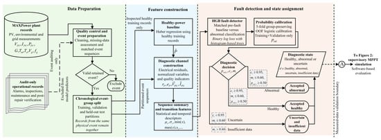
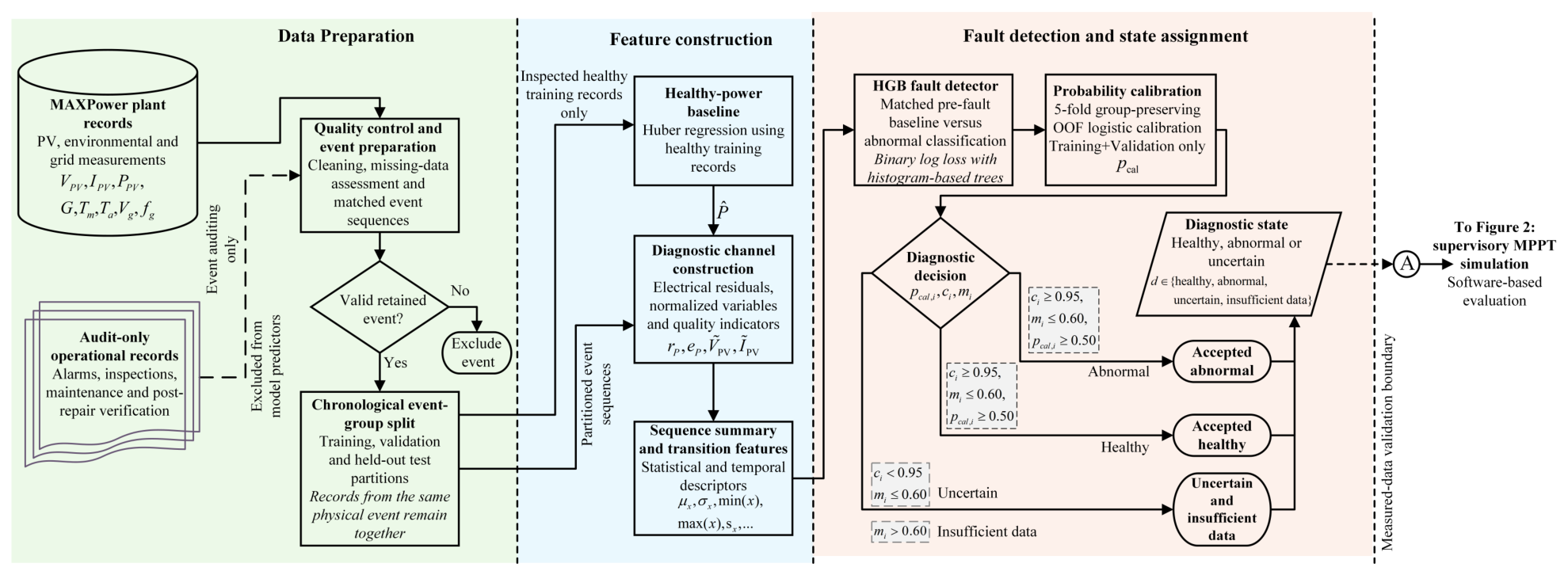
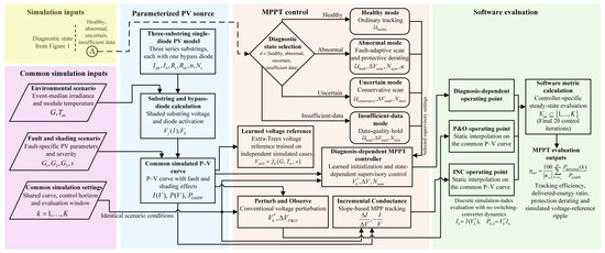
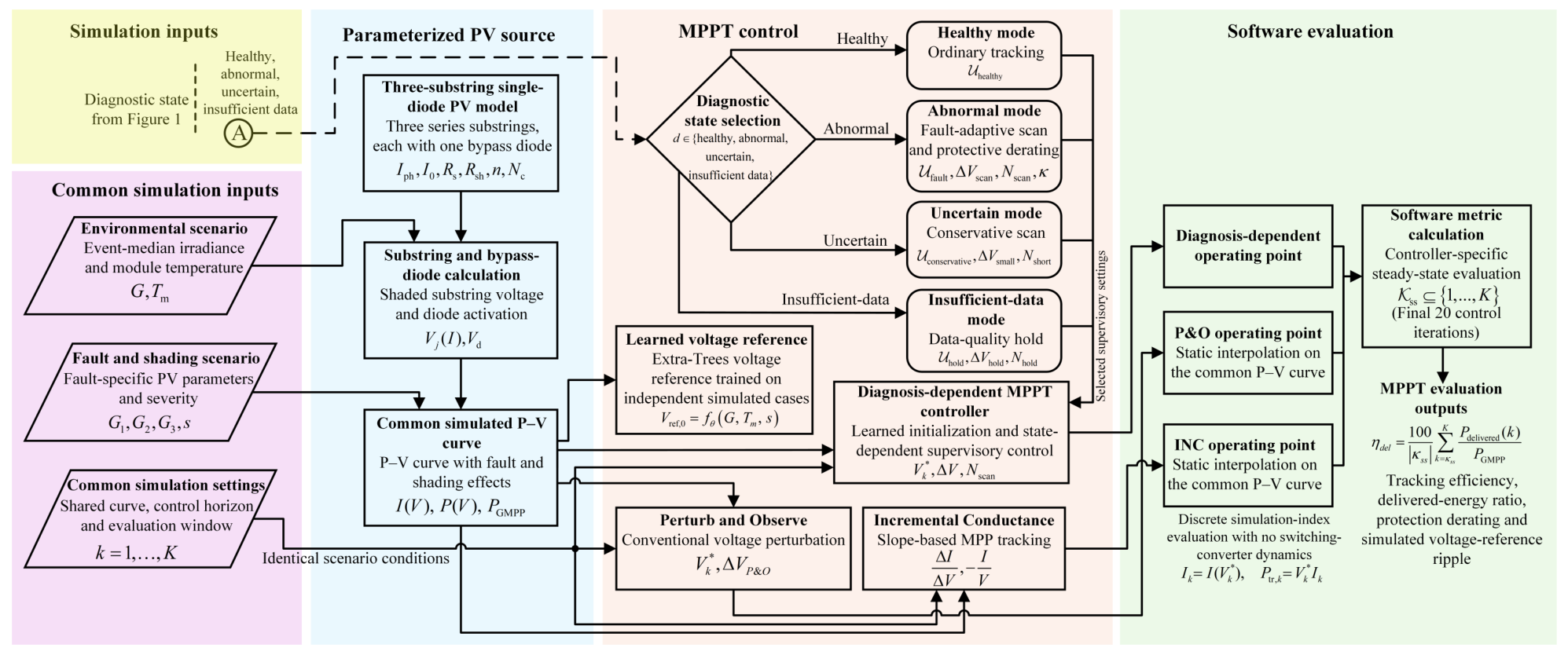
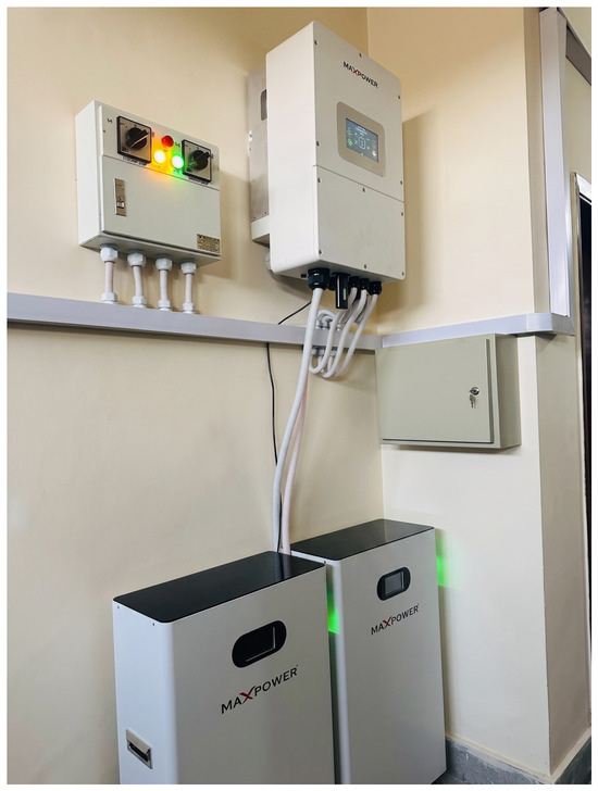
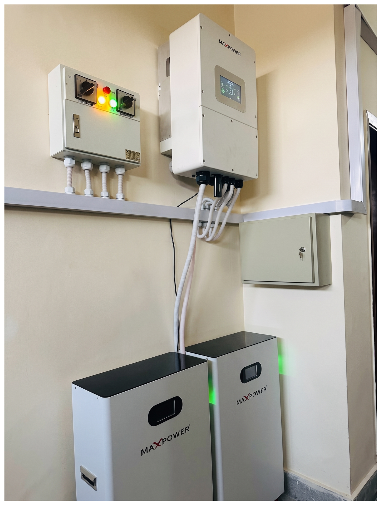
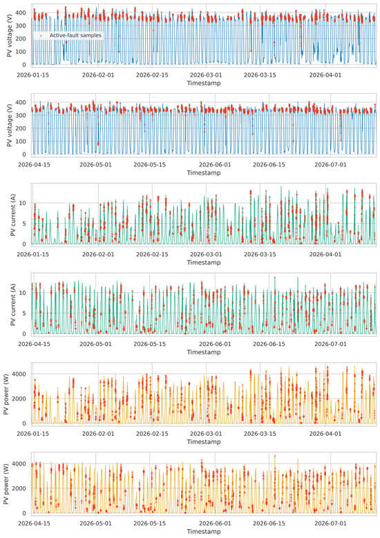
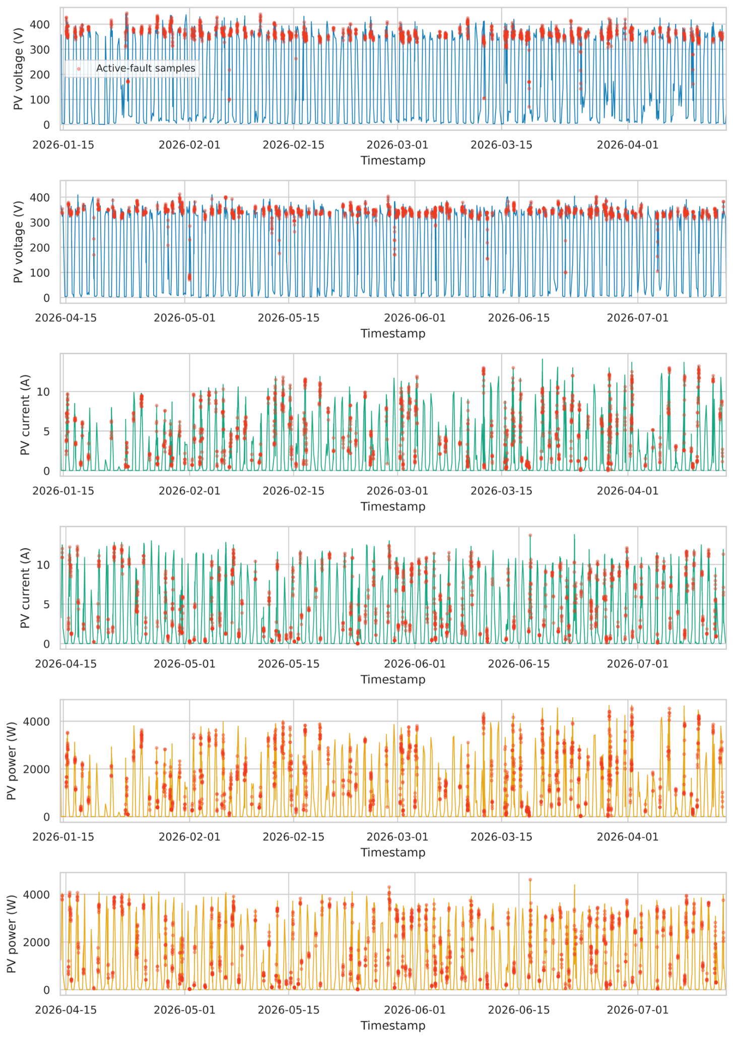
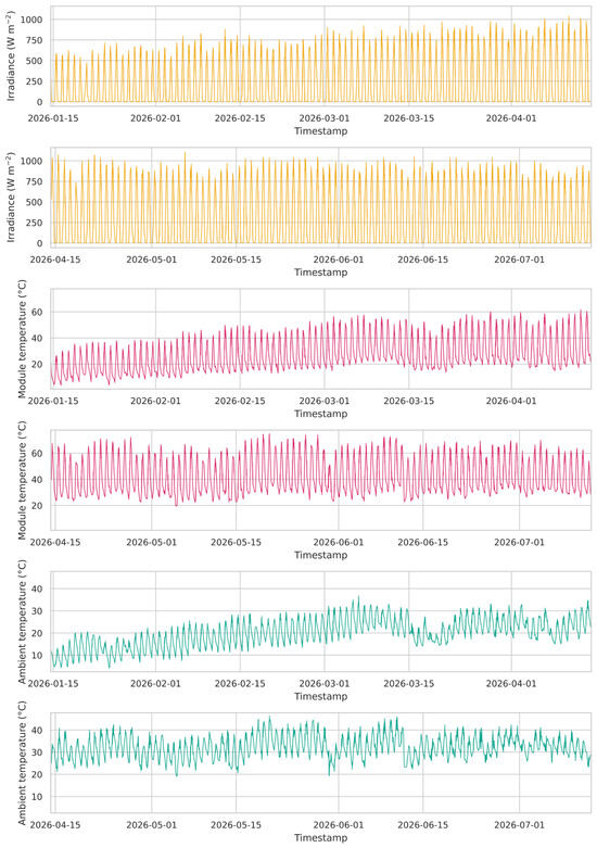
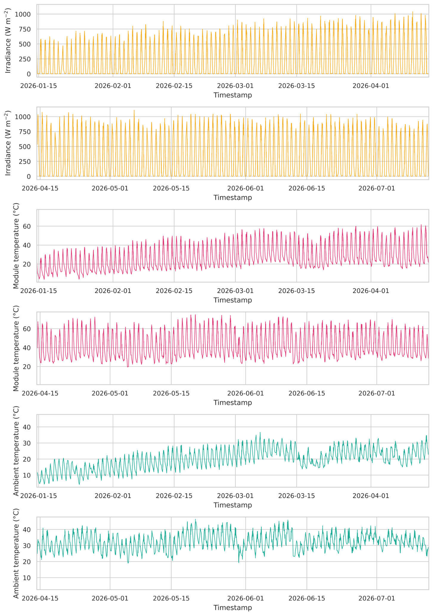
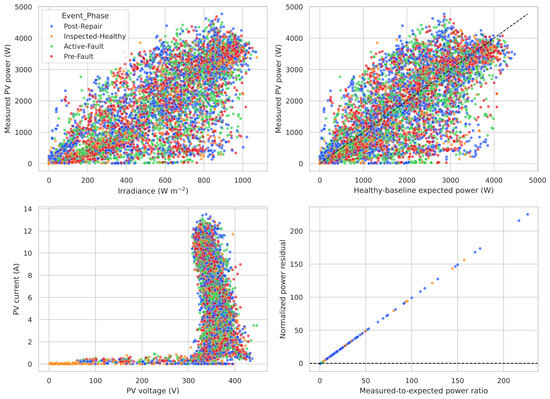
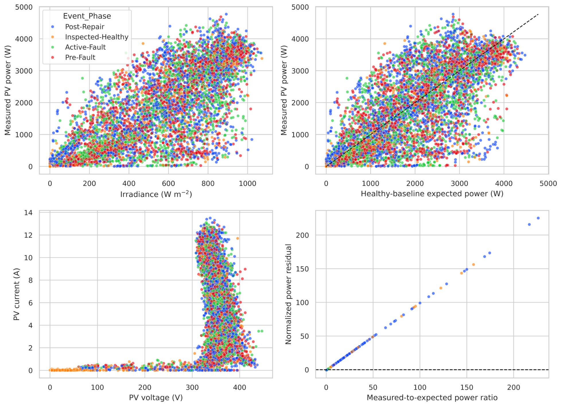
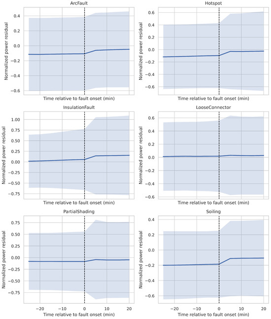
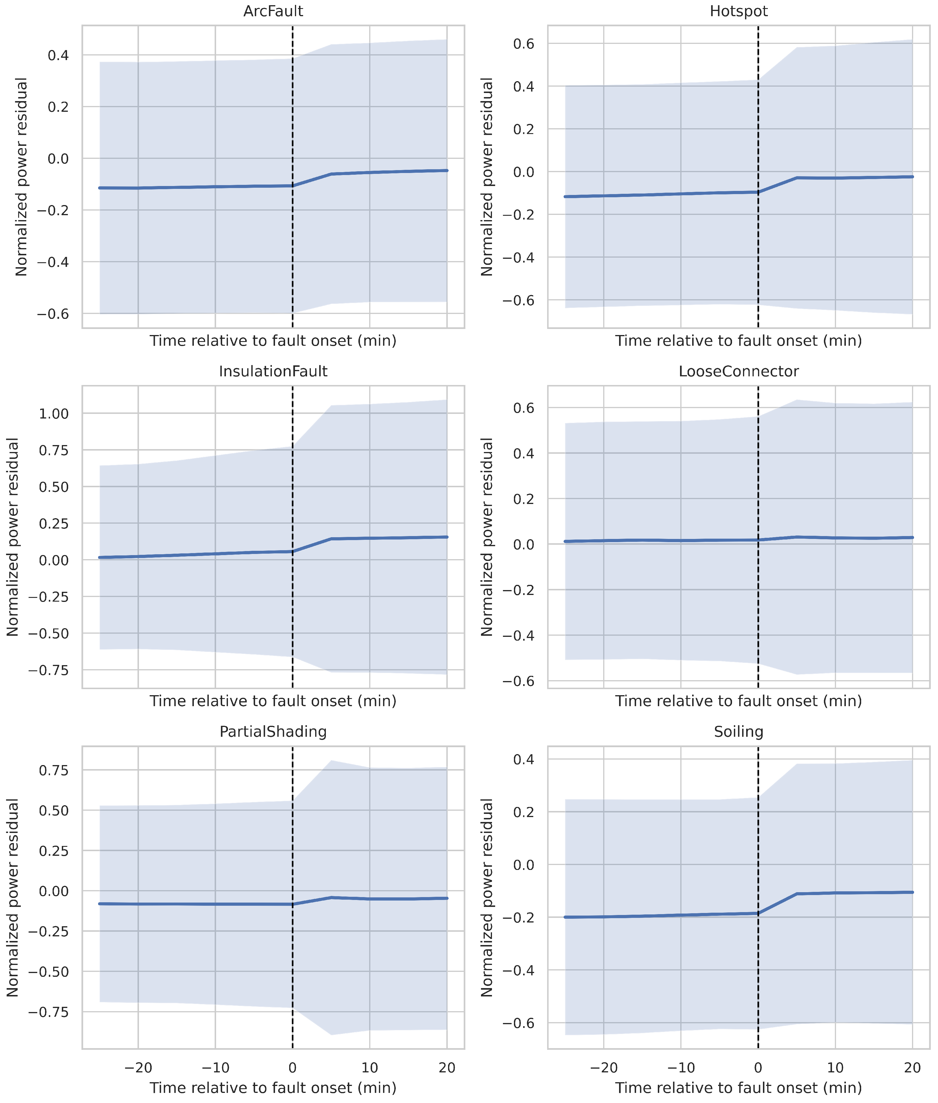
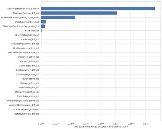
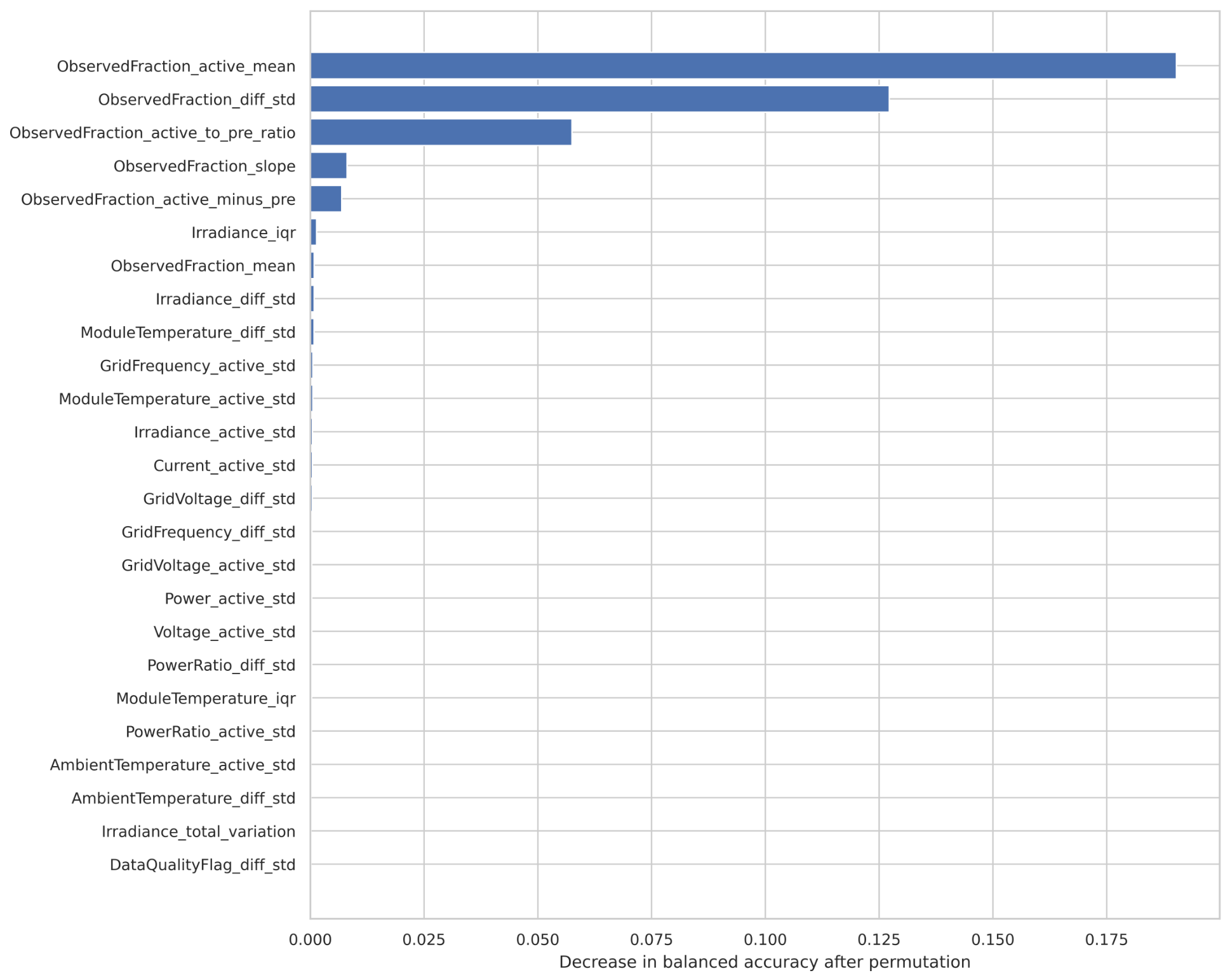
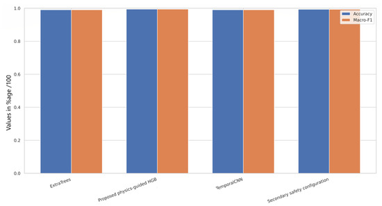
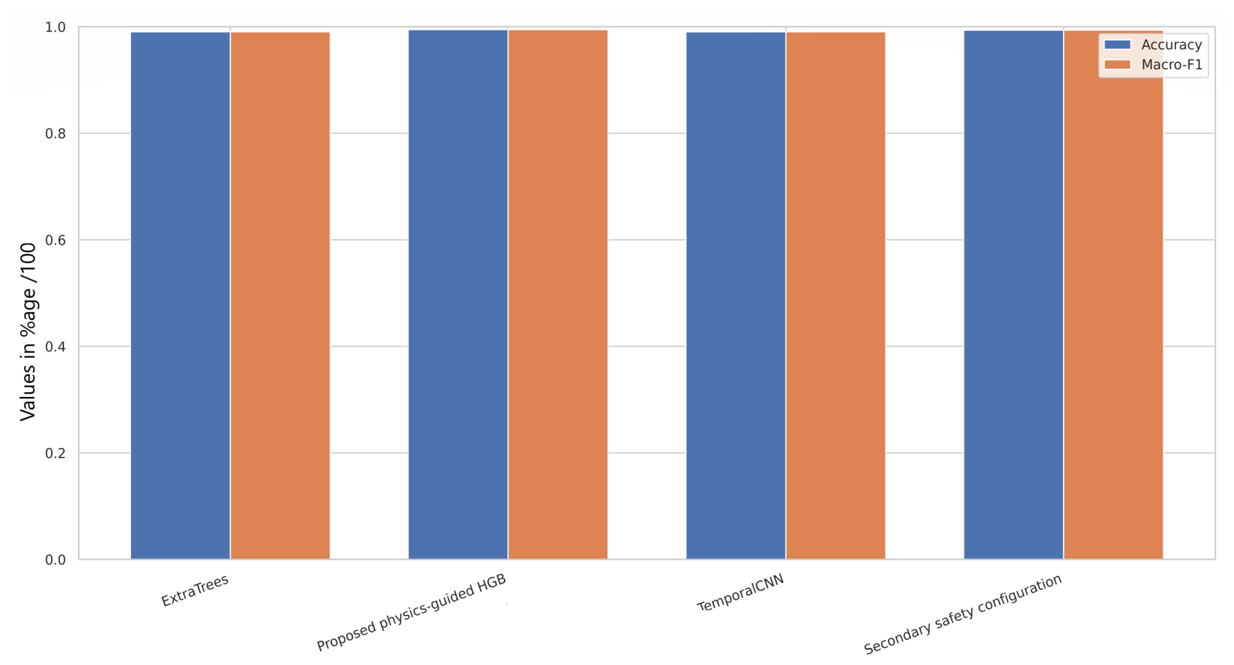
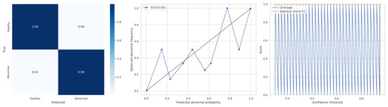
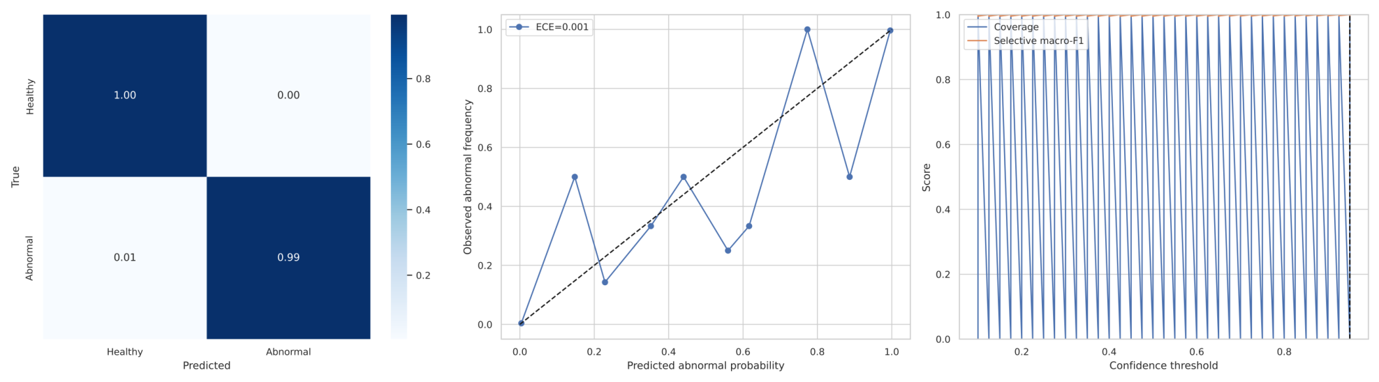
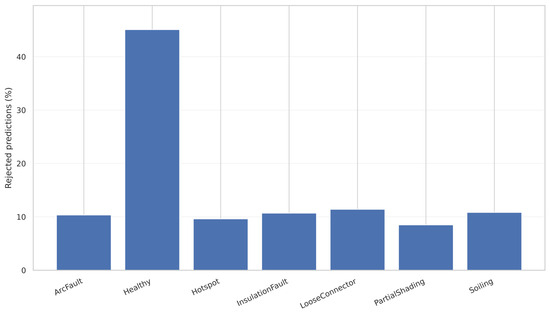
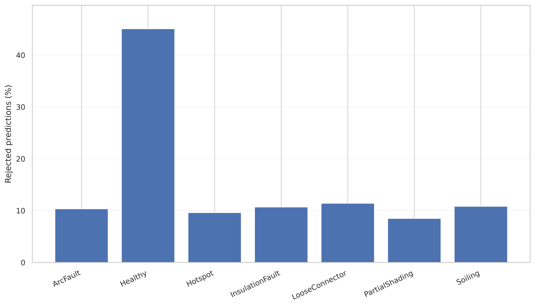
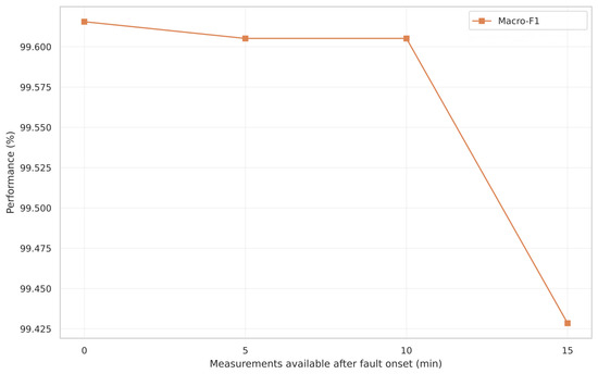
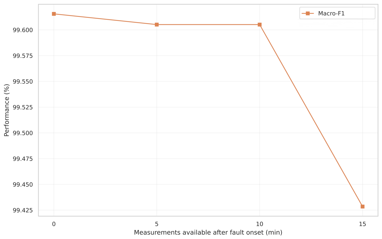
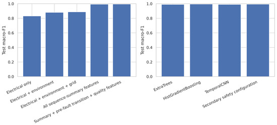
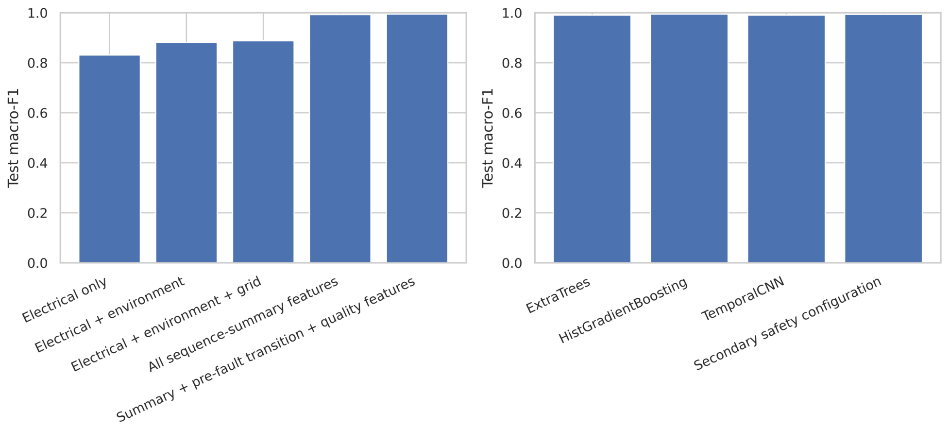
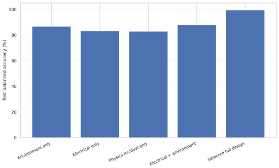
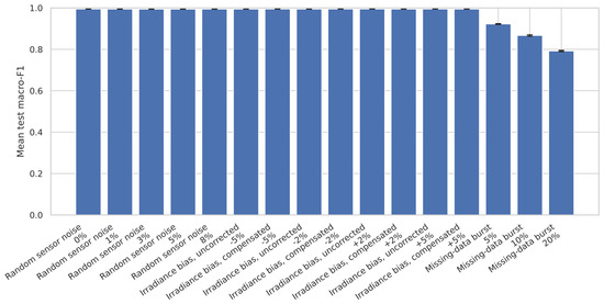
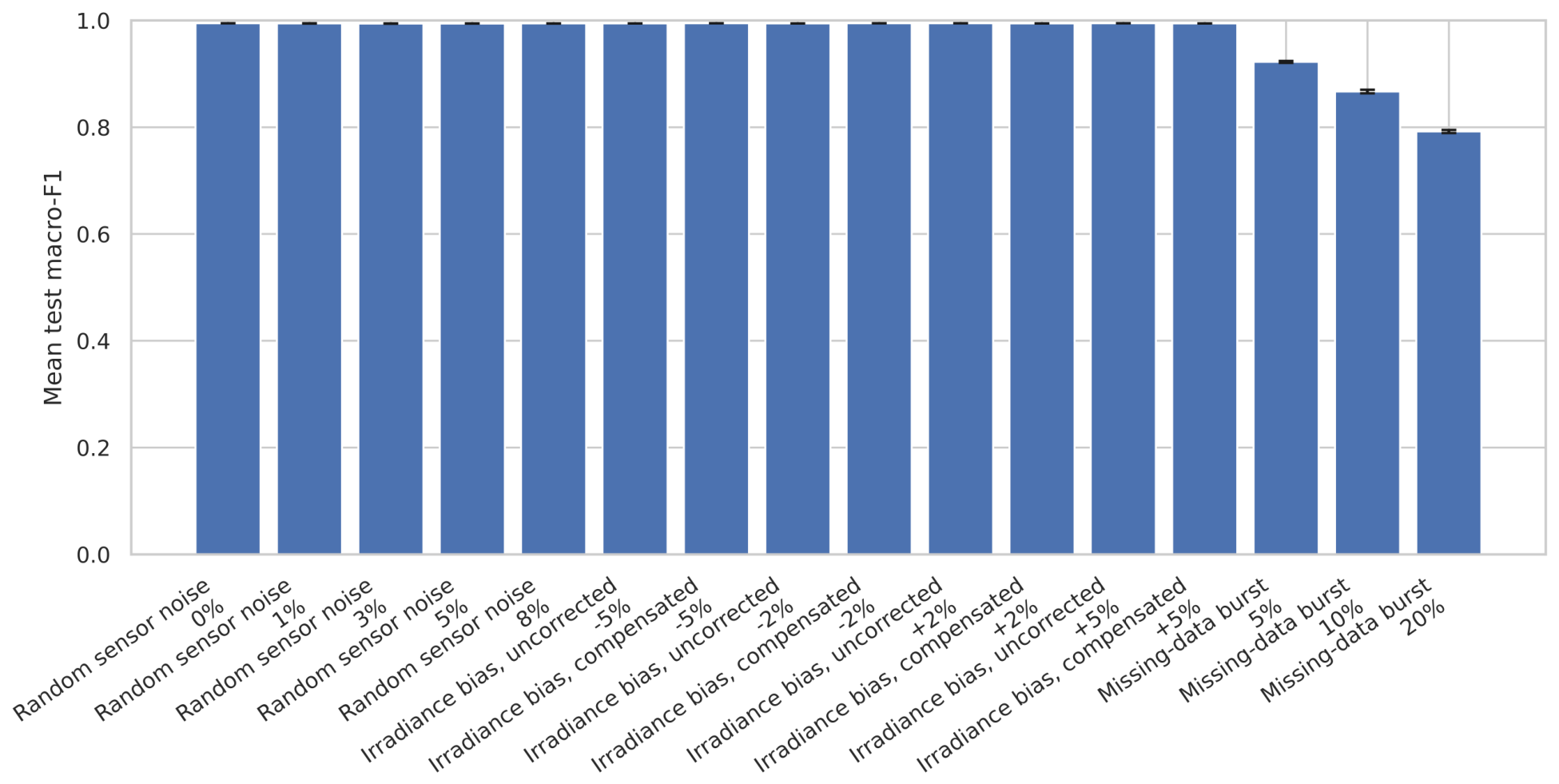
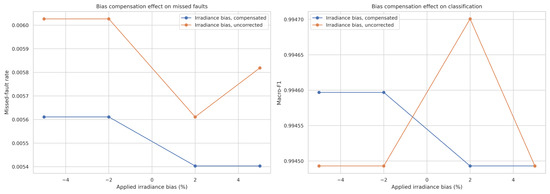
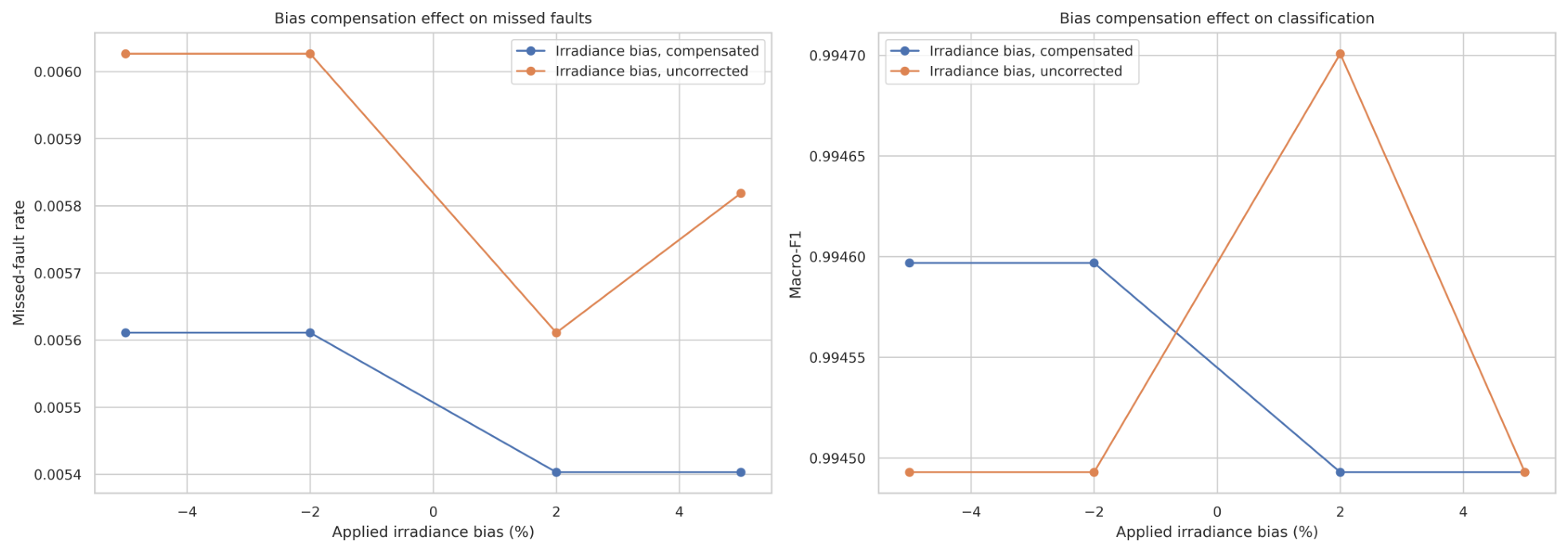
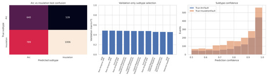
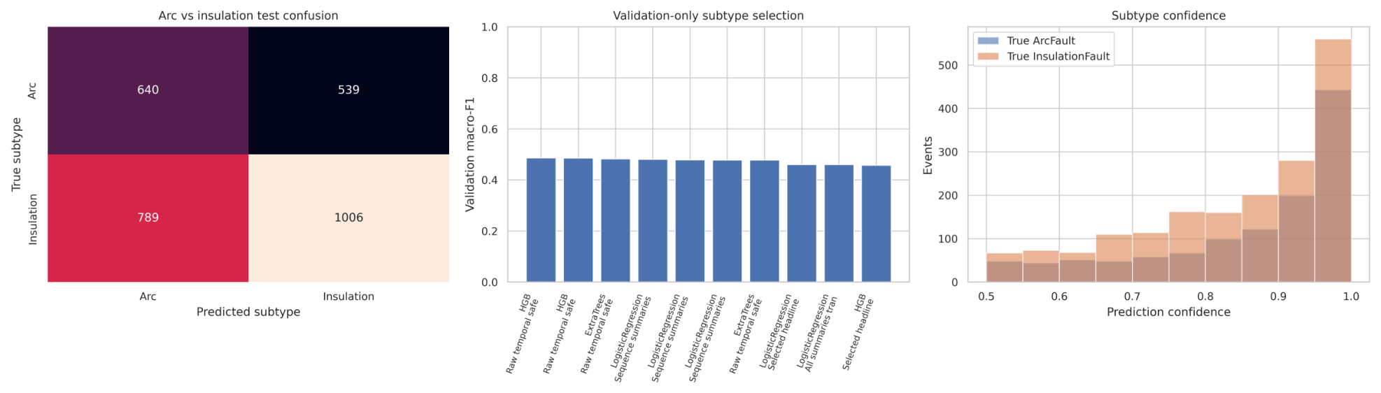
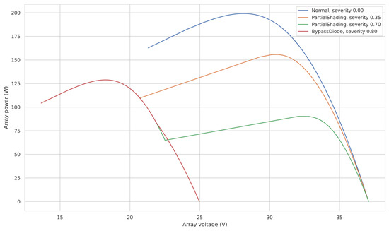
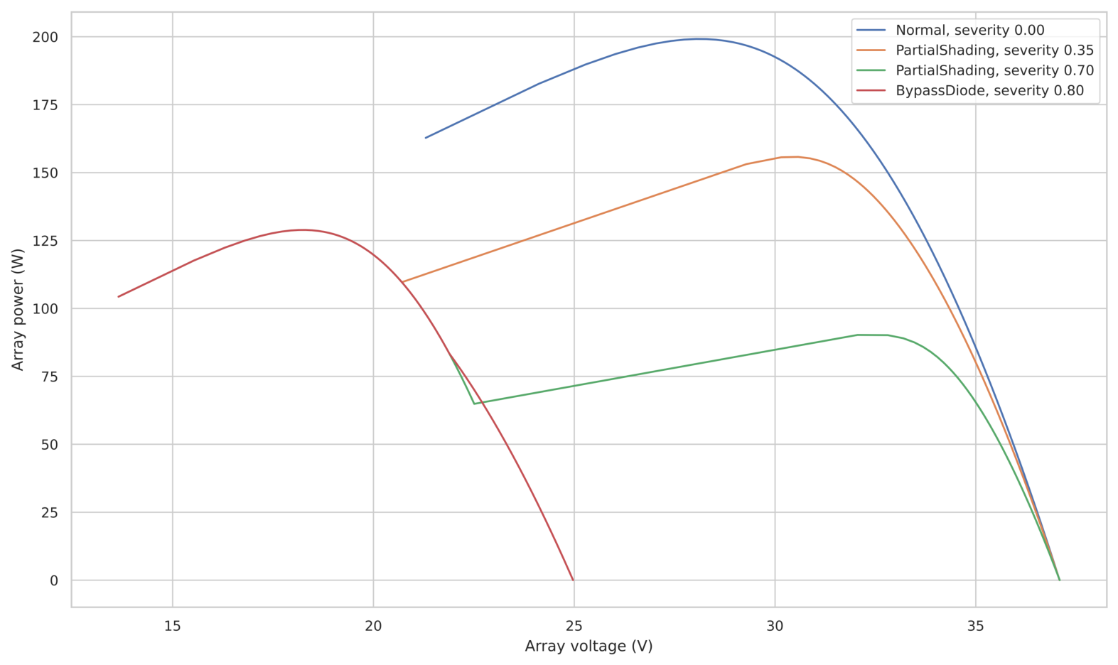
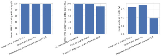
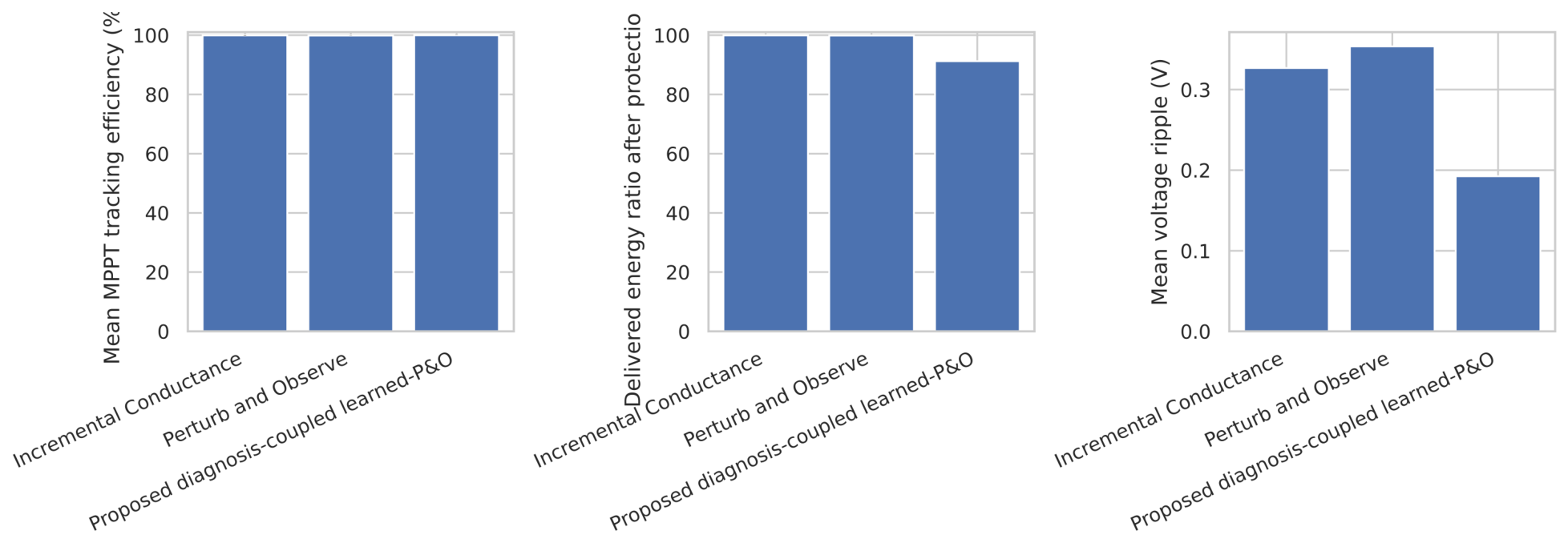
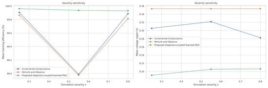
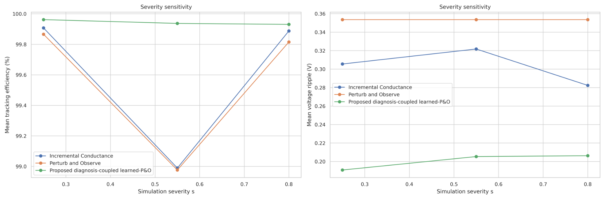
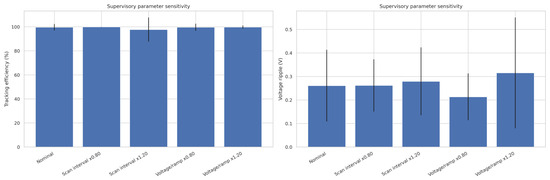
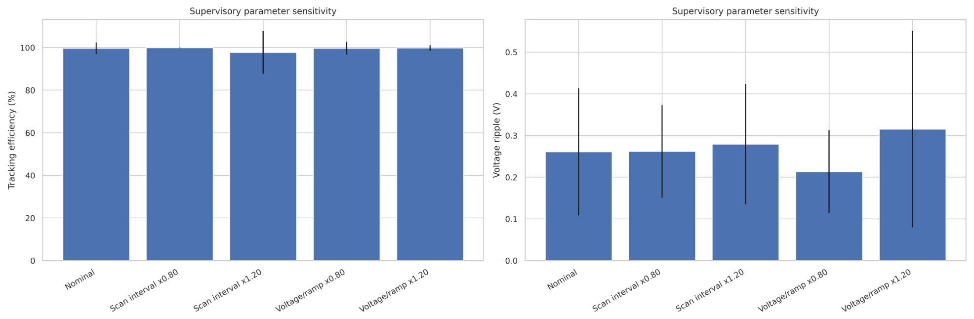
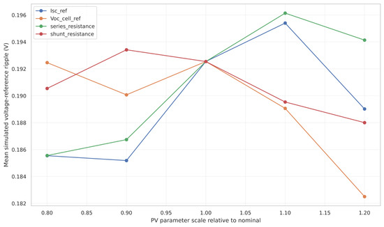
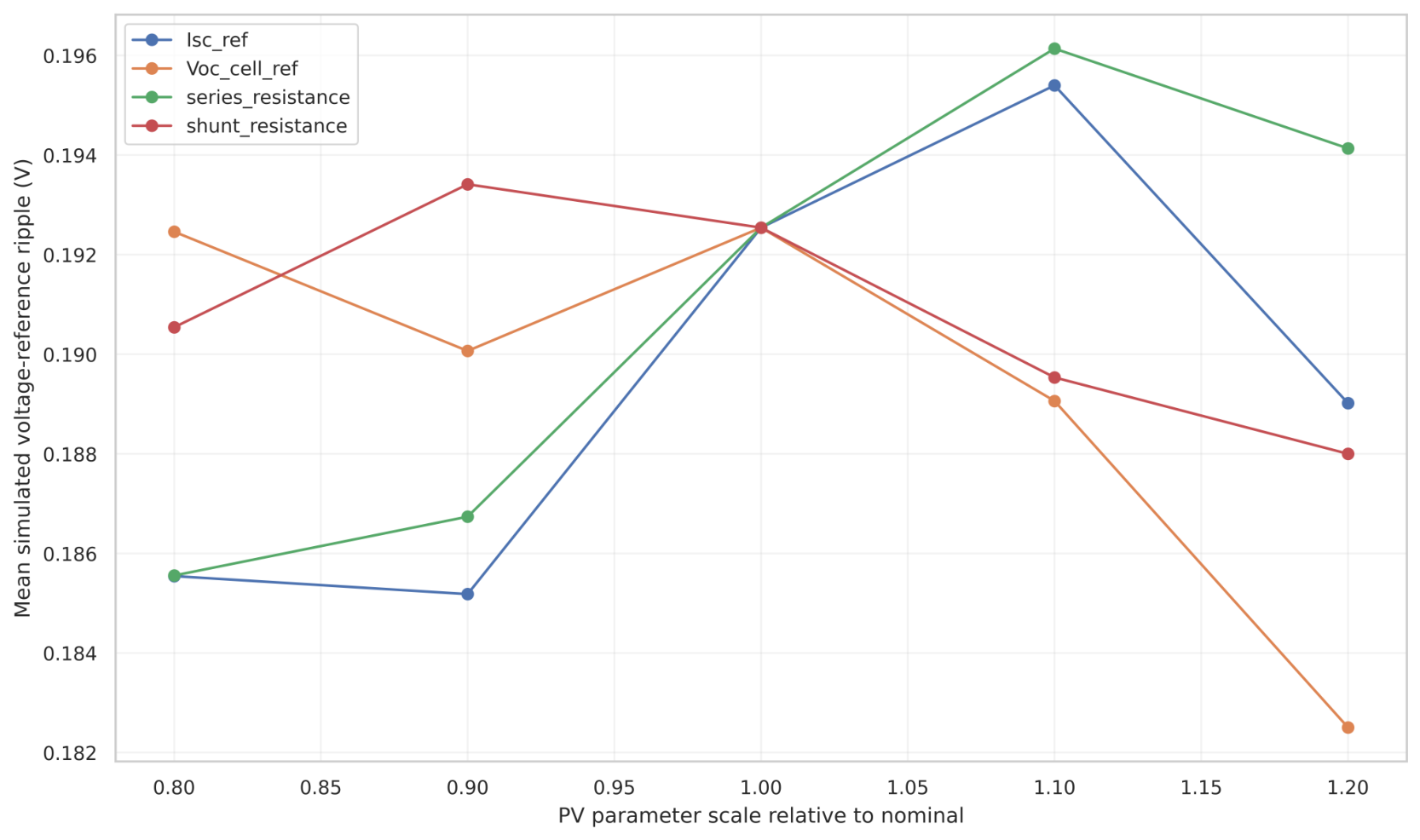
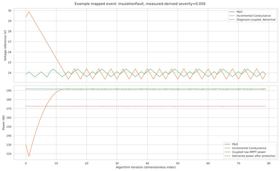
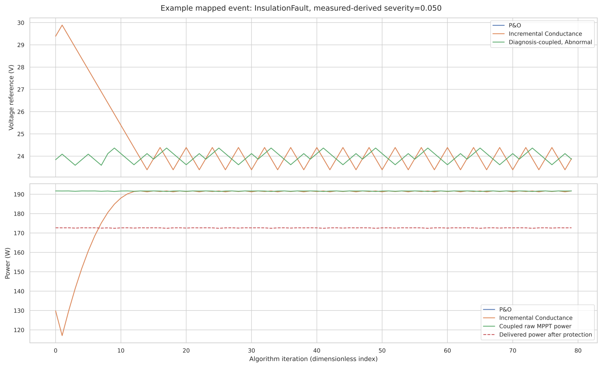

Disclaimer/Publisher’s Note: The statements, opinions and data contained in all publications are solely those of the individual author(s) and contributor(s) and not of MDPI and/or the editor(s). MDPI and/or the editor(s) disclaim responsibility for any injury to people or property resulting from any ideas, methods, instructions or products referred to in the content. |
© 2026 by the authors. Licensee MDPI, Basel, Switzerland. This article is an open access article distributed under the terms and conditions of the Creative Commons Attribution (CC BY) license.