Horizon-Dependent Model Ranking Reversal in Short-Term Load Forecasting: A Controlled Benchmark of Deep Learning Architectures

Abstract

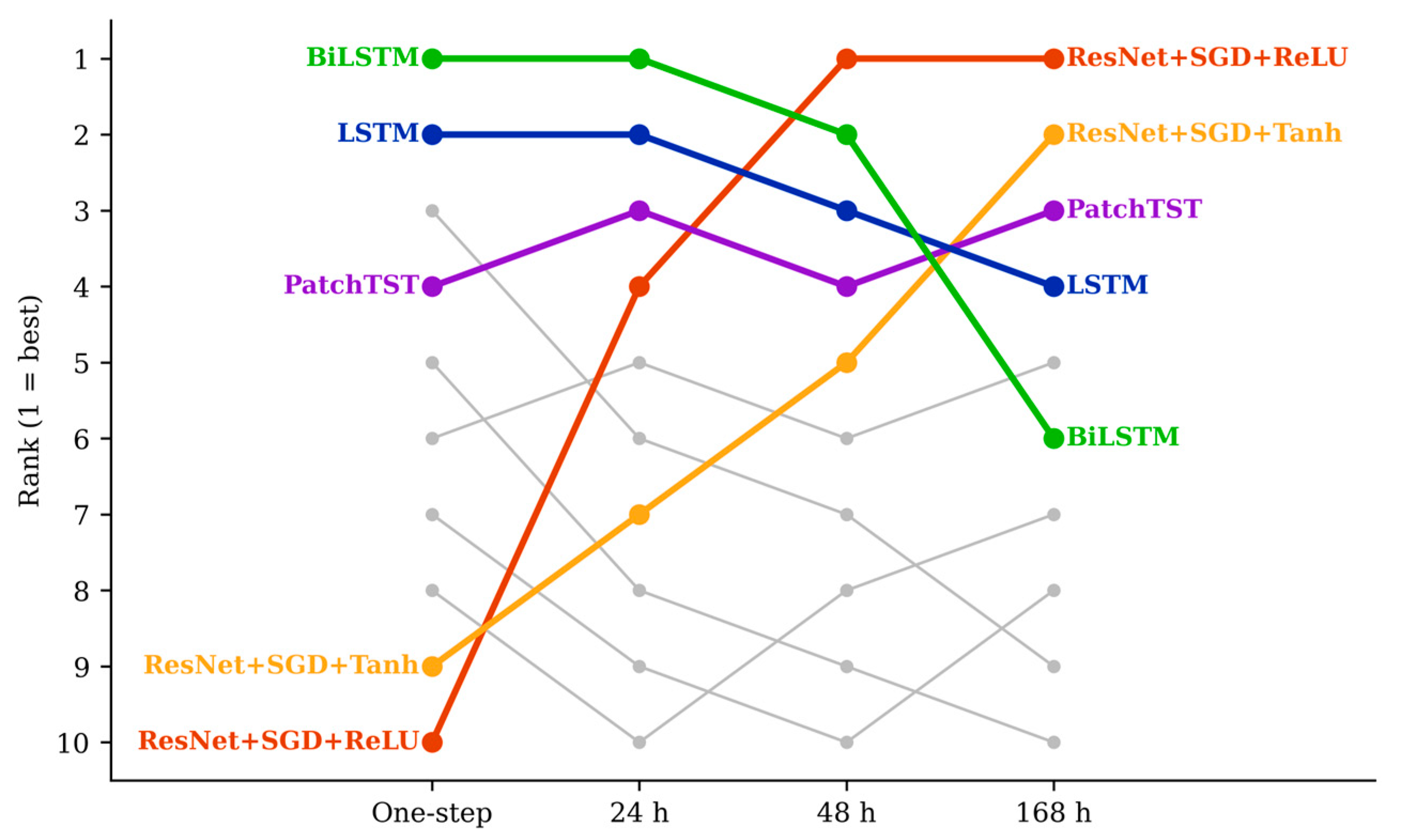
Short-term electricity demand forecasting is essential for power grid stability and generation scheduling. Although forecasting models are commonly evaluated using one-step-ahead predictions, high accuracy at a short horizon does not necessarily imply robust performance when forecasts are recursively extended over longer horizons. This study systematically investigates this issue by evaluating ten deep-learning models: recurrent architectures (LSTM, GRU, and bidirectional LSTM), four ResNet variants with different optimizer–activation configurations, two ResNet-based hybrid models, and the PatchTST Transformer. To ensure a fair assessment, all models are trained and evaluated using identical datasets, experimental settings, and training budgets. Their performance is assessed for one-step-ahead forecasting and recursive multi-horizon forecasting at 24, 48, and 168 h, with each experiment repeated over six independent random seeds. The results reveal a substantial reversal in model ranking as the forecasting horizon increases. For the next single step, the recurrent models are the most accurate, with the lowest mean average percentage error (MAPE), while the ResNet models trained with the SGD optimizer are the weakest. As the horizon extends to 168 h, the ranking reverses, and the two SGD-trained ResNets with ReLU and tanh activation functions rise to first and second rank, respectively, while the three most accurate one-step models fall to 6th, 4th and 9th rank with respect to MAPE. The more complex PatchTST transformer never leads. Therefore, demand forecasting models should be evaluated at the operational forecasting horizon for which they are intended to be deployed rather than selected solely based on one-step accuracy.

1. Introduction

Electricity demand forecasting is the backbone of power system operation, which allows power distributors, system operators, energy marketers, and utility organizations to match energy production and consumption, schedule production, and prepare a merit order list. Load forecasting on short-term time horizons from 1 hour (h) to several days is crucial in the operation of electricity grids [1]. Inaccurate forecasts are paid both in case of over-generation and under-generation. Over-generation results in unnecessary consumption of fuel and pollution, whereas under-generation poses threats to the reliability of supply. With the increasing number of renewable generators, electric vehicles, and energy resources, demand forecasts have become increasingly difficult to estimate, which makes short-term demand forecasting a critical research issue [2,3].

In time-series forecasting, the forecast horizon is the length of time into the future for which the model generates predictions, measured from the time at which forecasting starts [4]. In practice, various techniques for short-term load forecasting are used. A one-step-ahead forecast denotes the prediction of the load at the next subsequent time step using previous values, without feedback of predicted values. A recursive multi-step forecast refers to the sequential application of the same one-step-ahead model, in which each predicted load value is subsequently used as an input to generate the next prediction. This approach is usually employed to obtain forecasts at 24, 48, and 168 h horizons. In contrast, a direct multi-horizon forecast predicts multiple future time steps simultaneously in a single model evaluation. The forecast origin is defined as the timestamp at which a recursive forecasting sequence is initiated. Multi-origin evaluation refers to the assessment of forecasting errors across these multiple origins rather than along a single forecast trajectory, thereby providing a more representative measure of model performance and its variability. A conditional forecast denotes a recursive forecast in which the actual recorded values of exogenous variables are provided at each future time step, while only the load demand is recursively predicted. Accordingly, all multi-horizon results reported in this study correspond to conditional forecasts. Finally, the look-back window represents the length of historical information supplied to the model [5].

2. Related Work

2.1. Traditional Forecasting Methods

Conventional methods of load forecasting use statistical and conventional time-series models. Autoregressive integrated moving average (ARIMA) was one of the extensively used methods previously for its simplicity and interpretability. It offered a mathematical framework to detect linear temporal dependencies in the demand data [6]. However, ARIMA models were less efficient in handling the non-linear trends in electricity demand because they relied on stationarity and linearity [7].

Multiple linear regression and the exponential smoothing models used exogenous variables, such as calendar effects and temperature, to improve their accuracy, but again were limited due to their linear nature. The support vector regression (SVR) offered non-linear mapping using the kernel, but the requirement of manual feature engineering and scaling challenges necessitated the move towards deep learning [4]. In their comprehensive review, Ullah et al. [5] confirmed that statistical methods provide interpretable and simple solutions. However, they struggle with the volatile, nonlinear, and high-dimensional nature of modern demand data, resulting in failure to capture intra-day variation and seasonal fluctuations simultaneously.

2.2. Machine Learning Approaches

Machine learning became popular when artificial neural networks (ANNs) outperformed conventional statistical models across forecasting horizons [4]. Nowadays, artificial intelligence and machine learning-based methods have gained much popularity in solving complex engineering problems [8,9,10]. Methods using ensemble approaches, such as Random Forests and Gradient Boosting, provide competitive accuracy and robustness, although conventional machine-learning models do not have built-in mechanisms for modeling sequential temporal dependencies. In [4], Mamun et al. stated that hybrid models combining more than one predictive algorithm consistently attain the lowest errors across benchmark datasets, laying the foundation for deep-learning hybrids. Ullah et al. [5] further demonstrated the effectiveness of intelligent STLF models, including decision trees, gradient boosting, support vector machines, and multilayer perceptrons. Their simulation study showed that hybrid CNN–LSTM models achieved superior forecasting accuracy compared with standalone models, with an RMSE of 538.71 and MAPE of 2.72% for one-step forecasting. These findings further support the growing adoption of deep-learning hybrid models in STLF. Machine-learning methods, such as support vector regression and shallow neural networks, improved their performance on nonlinear and high-dimensional demand data with intra-day variation and seasonal fluctuations but still required manual feature engineering and struggled to capture long-range temporal dependencies [4,5].

2.3. Deep Learning for Electricity Demand Forecasting

Deep learning has reformed electricity demand forecasting by learning features directly from raw sequences. LSTM networks became the leading architecture for demand forecasting [11,12,13,14], followed by convolutional models [15,16,17], residual networks [18], convolutional–recurrent hybrids [1,19,20], and, most recently, attention-based transformers [21,22]. Hochreiter and Schmidhuber [11] introduced Long Short-Term Memory (LSTM) models, which resolved the issue of vanishing-gradient of standard recurrent networks through gated memory cells and gained widespread adoption. Kong et al. [13] further explained their superiority over conventional models for residential demand forecasting. Torres et al. [12] achieved errors less than 1.5% when tested on Spanish consumption data. Gated Recurrent Units (GRUs) [23] used fewer parameters and achieved comparable accuracy. Conv1D-based convolutional neural networks (CNNs) proved effective in extracting local temporal patterns. This was further demonstrated by Kim and Cho [15] that CNN-LSTM hybrids outperform their standalone models. Zhang et al. [16] suggested a CNN-LSTM multi-task model. Wan et al. [17] included attention mechanisms. The strength of convolutional–recurrent combinations was further established by Sekhar and Dahiya [24] and Goh et al. [25]. Vangipuram and Giridhar [14] demonstrated that weather-based embeddings remarkably improved forecast accuracy. Dewangan et al. [26] merged signal decomposition with LSTM and achieved 1.567% MAPE on Indian data.

2.4. Residual, Hybrid, and Transformer Architectures

Deep residual networks (ResNets) were initially introduced by He et al. [18] for image classification. After their subsequent improvement by [27], they were later used for sequential data. Residual skip connections help gradient flow through the network. This supports the training of deeper architectures without decreasing performance. Chen et al. [28] used these architectures for electricity demand forecasting and obtained better accuracy than standard CNNs. Chen et al. [1] used an Australian dataset (2006–2010) to apply a ResNet-LSTM hybrid model and reported strong forecasting accuracy. Related hybrids include Albelwi’s ResNet-LSTM with Huber loss [19], the residual-LSTM framework of Sheng et al. [20], and the Inception-embedded ResNet of Mirza et al. [29]. The complementary strengths of convolutional-residual and recurrent components have motivated extensive research on hybrid deep learning models [1,2,19,20]. Ozen et al. [2] fused LSTM, CNN and transformer components. Asiri et al. [3] established hybrid superiority for smart-grid STLF. Jang et al. [30] found CNN-LSTM hybrids to achieve the lowest errors in a comparative study. Most recently, transformer-based models have emerged as competitive alternatives: Vaswani et al. [21] introduced the attention mechanism, and Pentsos et al. [22] proposed a hybrid LSTM-Transformer that outperformed standalone LSTM, BiLSTM, and full-transformer baselines on U.S. residential data. Singh et al. [31] established early neural-network benchmarks on Australian data, and Al Khafaf et al. [32] applied deep LSTM to Australian smart-meter data for multi-day forecasting.

2.5. Multi-Step Forecasting and Recursive Error Propagation

The difference between direct multi-step and recursive forecasting has been studied extensively outside load forecasting. Ben Taieb and Atiya [33] provide a bias-variance analysis of direct multi-step versus recursive estimation and show that the recursive method inherits a bias that compounds with the horizon. Ben Taieb et al. [34] provide an empirical comparison of the principal strategies across a large collection of series. Marcellino, Stock & Watson [35] provide comparable conclusions for iterated versus direct forecasting in macroeconomic settings. More recently, these strategies were applied within energy forecasting [36,37].

2.6. Research Gaps and Contributions

Despite the considerable literature on deep-learning demand forecasting [4,5,7,12,38,39], several gaps remain to be filled.

• First, complex hybrid and transformer models are rarely compared against simple recurrent baselines under genuinely identical conditions, leaving it unclear whether their added complexity delivers consistent gains.
• Second, the impacts of training design, importantly optimizer selection, in the residual forecasting models have not been thoroughly investigated, although it can have a substantial impact on the output.
• Third, and most importantly for the present study, models are rarely compared across multiple forecast horizons under identical conditions. Most studies evaluate and rank models on one-step-ahead accuracy alone. Yet operational forecasting rarely stops at one step, as grid operators require forecasts hours and days ahead, produced by rolling a model forward on its own predictions. That recursive forecasting accumulates error is well established; what remains to be established is whether this accumulation is uniform across architectures, or whether it is severe enough to reorder them. If the ordering is not preserved, then a model selected on one-step accuracy may not be the model best suited to the horizon at which it is deployed.

In this paper, the contribution is an unbiased and controlled reply to fill the above three gaps. Rather than designing a new model, a wide variety of existing deep learning models, including residual, recurrent, transformer and hybrid, have been compared under identical conditions in this study. These models are evaluated one step ahead, as well as over several-hour time horizons. Further, the average scores are calculated based on multiple random seeds in order to distinguish real from chance. The main outcome of the study is the ranking of deep learning forecast models based on the forecast horizon. Models that lead at single-step forecasts can fall well down in the performance ranking at multi-step forecasts. Similarly, the models that are weakest at one step can rise in the ranking in multi-step forecasts. One-step accuracy is therefore a weak predictor of recursive multi-horizon accuracy.

It is pertinent to note that this study employs a recursive multi-horizon forecast to predict demand at the next intervals. The direct multi-horizon forecast, which predicts multiple future time steps simultaneously in a single model evaluation, is not the scope of this study. Similarly, multi-horizon forecasts computed in this study are conditional forecasts, where future weather, price and calendar values are taken as known.

3. Methodology

3.1. Model Input and Output

This paper addresses short-term electricity demand forecasting as a supervised sequence-modeling problem. In the one-step regime, the model predicts demand conditional on recent observed conditions rather than from past demand only. In the recursive multi-horizon regime, only the demand channel is fed forward; the weather, price and calendar features take their actual recorded values at every rollout step. Each trained model is tested in two different ways: to predict one step from the observed inputs and to be rolled forward over many steps on its own output.

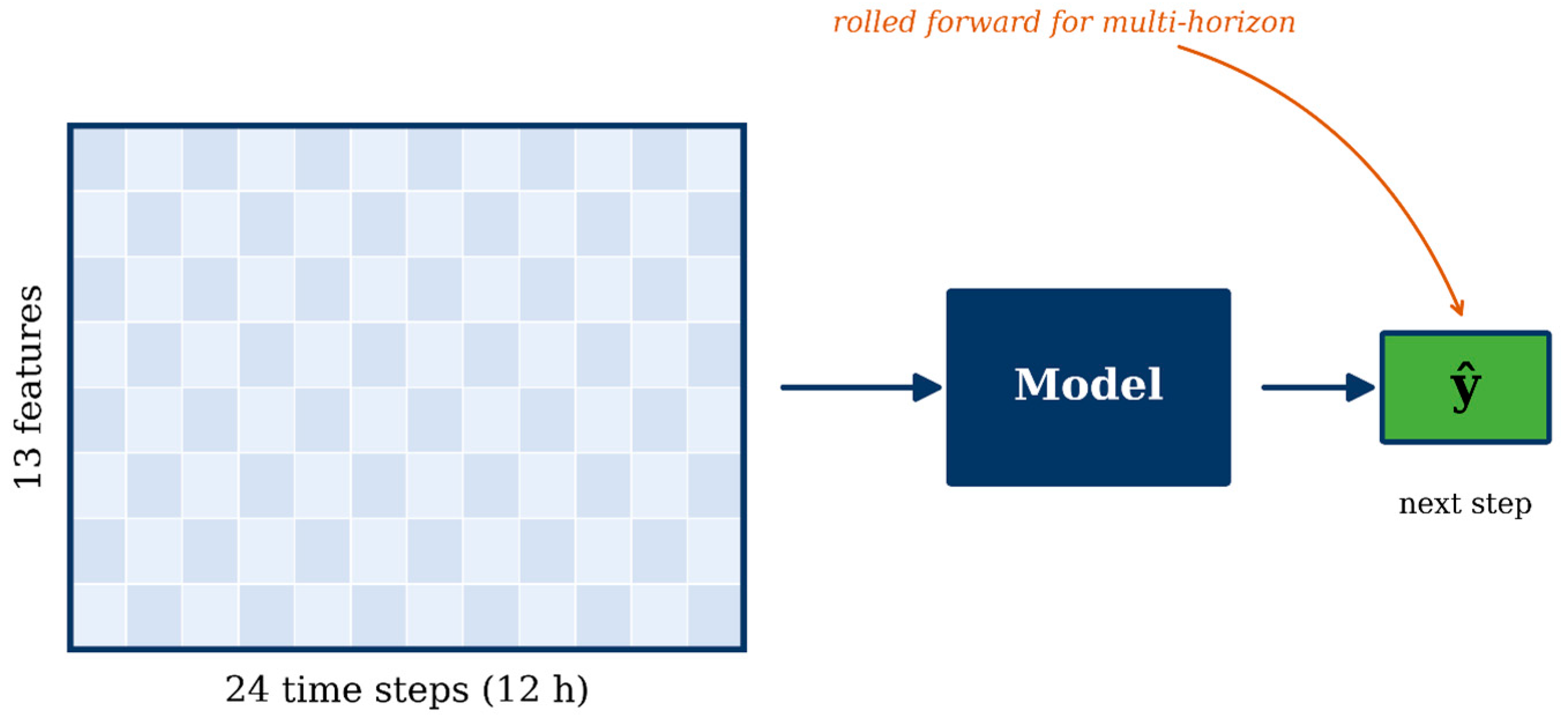
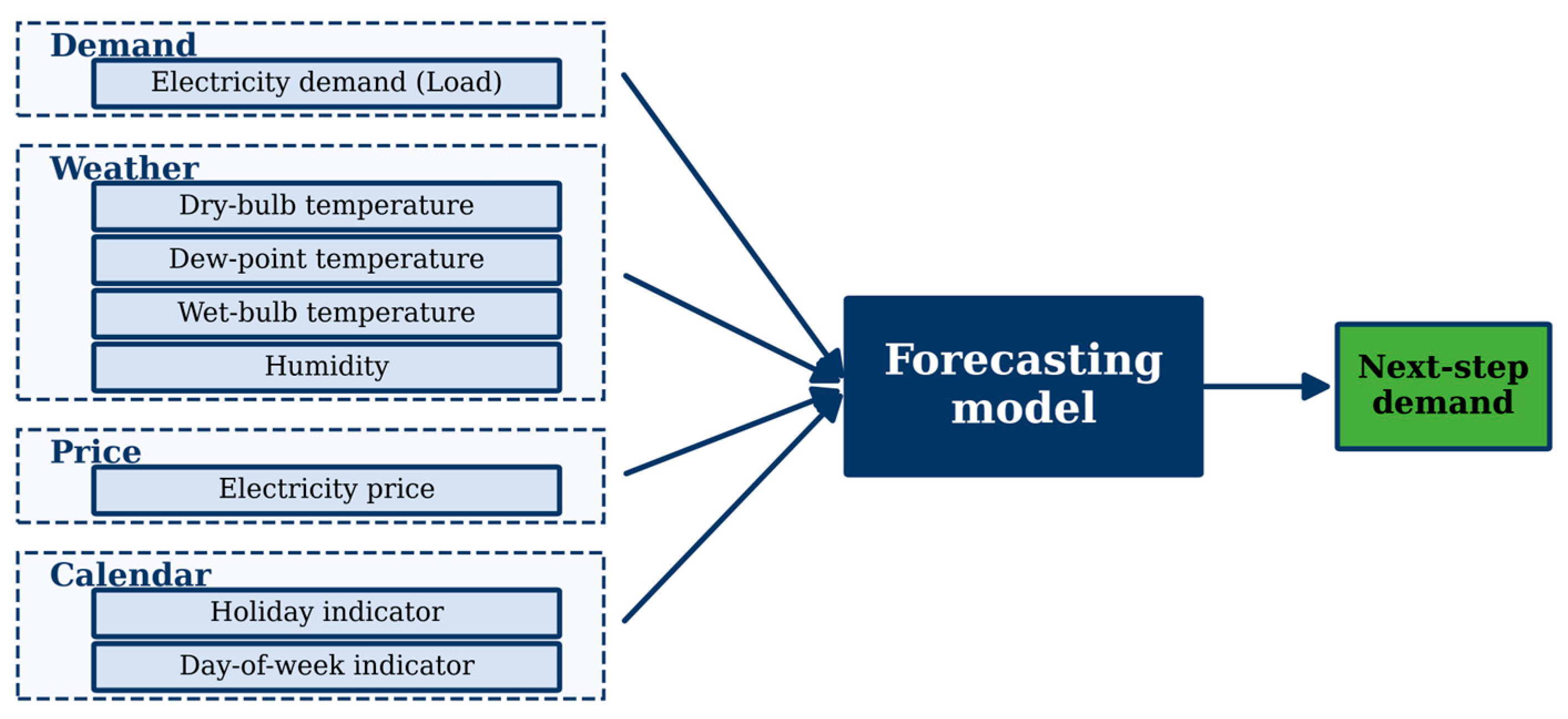
Each input sample consists of a look-back window of 24 consecutive half-hourly time steps (12 h). At each time step within the input window, the model receives a 13-dimensional feature vector: the recent electricity demand (load), four meteorological variables (dry-bulb temperature, dew-point temperature, wet-bulb temperature, and humidity), the electricity price, and one-hot calendar indicators for public holidays and day-of-week. The model output is a single scalar—the forecasted demand for the next 30 min step, as shown in Figure 1. From Figure 2, it is evident that a 24-step × 13-feature look-back window of input is mapped to a single next-step demand output, which is rolled forward for multi-horizon forecasting.

The feature set follows the benchmark study [1] so that results are directly comparable. However, this work uses actual values for exogenous variables such as price and weather parameters at every rollout step, assuming their operational availability. This assumption reduces absolute errors relative to actual deployment and is used for all ten models identically. Hence, the accuracy of every model is inflated by approximately the same amount without favoring any architecture in the ranking mechanism. It is worthy to mention that the availability of electricity price as a forecasting input is not universal, as it depends on the market structure. Actual prices are usually not known seven days ahead when a forecast is issued. Moreover, a vertically integrated utility has no equivalent public market price for its native load. Price is partly determined by the same system conditions that drive demand, and is therefore not necessarily an independent predictor. In this study, we are using the actual price and weather parameters rather than the predictive values. Practically, it will contribute little to our models because the Queensland price series has rare spikes and is close to constant across the great majority of intervals after normalization.

3.2. Forecasting Task

For the multi-horizon regime, the one-step prediction is recursively fed back to form the next input window, while the exogenous features take their actual values. Mathematically, it can be given by the following:

$${\widehat{y}}_{t+k}=\left(X_{t+k-1},e_{t+k}\right),\hspace{1em}\hspace{1em}k=1,\dots ,H$$

(1)

where

• $X_{t+k-1}$ is the updated input window containing actual historical load values and previous predicted load values,
• ${\mathrm{e}}_{\mathrm{t}+\mathrm{k}}$ represents the known future exogenous features at time $t+k$ and
• $H$ is the forecast horizon.

After each prediction, the window is updated by appending ${\widehat{y}}_{t+k}$ together with the corresponding exogenous features:

$${\widehat{x}}_{t+k}=\left[{\widehat{y}}_{t+k},e_{t+k}\right]$$

(2)

In this work, the predicted demand at each step is appended to the next input window, together with the actual exogenous features. Starting from each forecast origin, the recursion defined in (1) was rolled forward to obtain the 168 h trajectory. Performance was then evaluated cumulatively at time horizons of 24, 48, and 168 h (48, 96, and 336 half-hour time intervals).

Two forecasting regimes have been considered in this work. The one-step regime is retained for continuity with prior work on this dataset, allowing the results to be compared with published one-step figures. The recursive regime is the main focus of this study because it is identical to real-world practice, where a load forecaster has to predict many steps ahead without having intervening demand values. The model produces forecasts up to 168 h (336 half-hour intervals). The results are calculated cumulatively at 24 h, 48 h, and 168 h, where the 48 h result contains the 24 h results, and the 168 h result covers a full week.

3.3. Training and Testing Partition

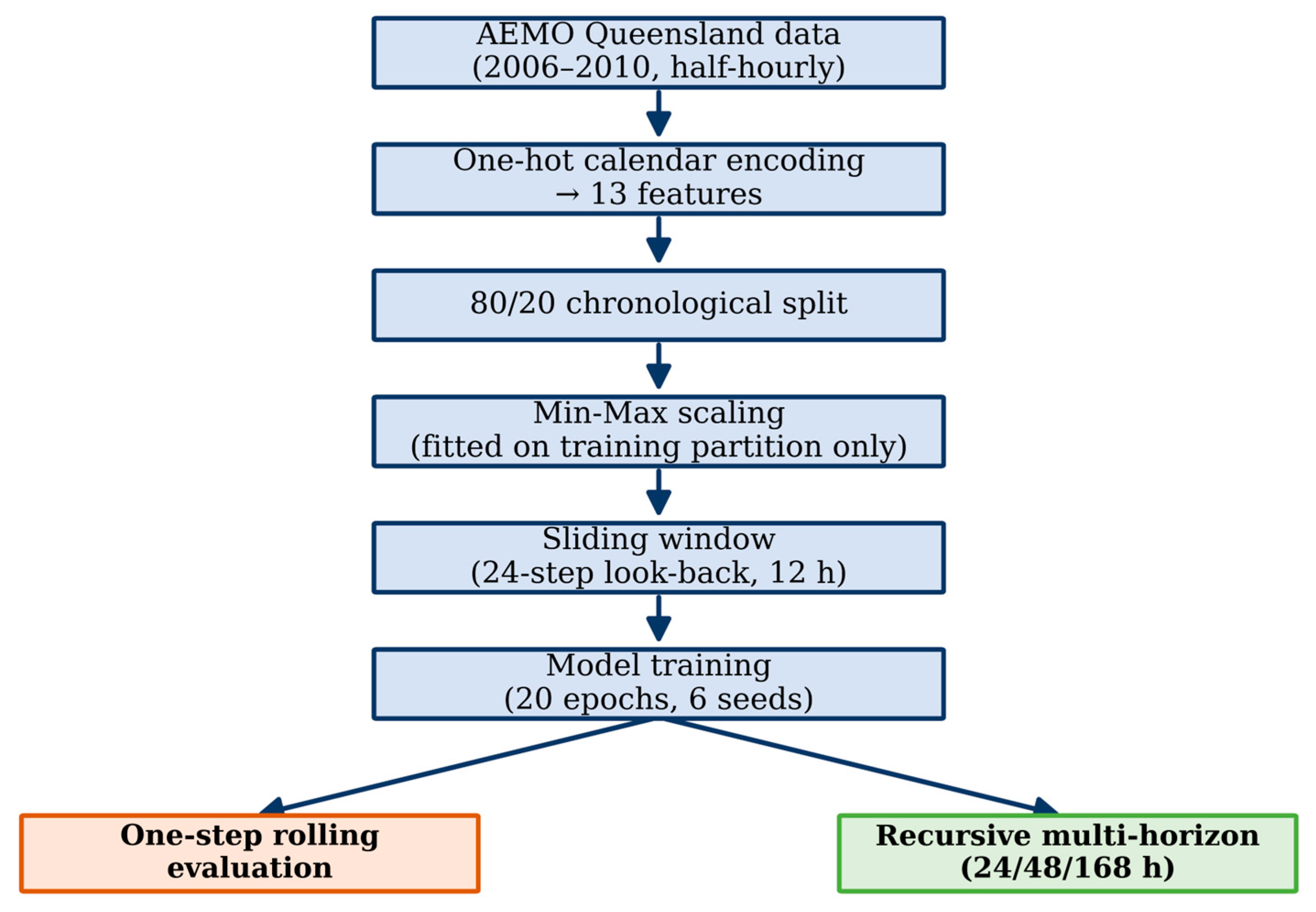
The dataset was split chronologically into 80% training and 20% testing subsets, as shown in the process flowchart shown in Figure 3. Data shuffling was kept disabled to preserve temporal sequence, which is required for time-series forecasting. It made sure that models were always trained on past data and tested on strictly future data. It also ensures the prevention of any leakage of future information into the training. This data split was used for the evaluation of all the models. By using this strategy, the effect of data partition on the results was eliminated. Only the model architecture and its training configurations were responsible for the differences in the results.

3.4. Data Preprocessing

All features were scaled to the unit interval using min-max normalization. The scaling constants were computed from the training partition only, and the resulting transform was then applied to the full series. This ensures that no information from the test period enters the fitted parameters. Furthermore, this prevents numerical instability during gradient-based optimization and ensures a fair comparison across features of differing magnitude. The transformation is defined as follows:

$$x_{scaled} = {\displaystyle \frac{x - x_{min}}{x_{max} - x_{min}}}$$

(3)

where $x_{max}$ and $x_{min}$ are computed from the training partition. Applying (3) to every feature, a sliding-window approach transformed the multivariate series into supervised samples: a look-back window of 24 time steps (12 h) was used, with each window predicting the subsequent 30 min electricity load demand value. As the meteorological and price features are included in every window, the input is multivariate with 13 features per step.

3.5. Model Architectures

Evaluation of ten deep learning models was conducted by processing their training and testing. These models represent four architecture groups, i.e., recurrent, residual, transformer and hybrid. LSTM, BiLSTM and GRU represent the recurrent family. The residual family was represented by four ResNet variants, which differ in optimizer and activation selection. Two hybrid models were used, which are ResNet+LSTM and ResNet+GRU. Finally, the transformer family was represented by PatchTST. All models use a 24-step (12 h) look-back, min-max scaling, 80/20 chronological split, 20 epochs, batch size 32, MSE loss, and six random seeds. The recurrent, residual, and hybrid models were implemented in Keras 3.13.2, TensorFlow 2.20.0 and PatchTST in PyTorch 2.10.0 (CUDA 12.8), with the same training budget. Each model was tested over six random seeds, with results reported as the mean and standard deviation.

Table 1. Architectural configuration of the ten evaluated models.

Model	Conv. Layers	Recurrent Layers	Optimizer	Activation	Regularization	Parameter Count
LSTM	—	2 × 64	Adam	tanh (gates)	Dropout 0.2	53,057
GRU	—	2 × 64 (GRU)	Adam	tanh (gates)	Dropout 0.2	40,193
BiLSTM	—	2 × 64 (bidir.)	Adam	tanh (gates)	Dropout 0.2	138,881
ResNet+SGD+ReLU	7 (3 blocks)	—	SGD	ReLU	Batch Norm	82,689
ResNet+SGD+Tanh	7 (3 blocks)	—	SGD	Tanh	Batch Norm	82,689
ResNet+Adam+Tanh	7 (3 blocks)	—	Adam	Tanh	Batch Norm	82,689
ResNet+Adam+ReLU	7 (3 blocks)	—	Adam	ReLU	Batch Norm	82,689
ResNet+LSTM	7 (3 blocks)	2 × 64	Adam	ReLU/tanh	BN + Dropout 0.2 (× 3)	148,737
ResNet+GRU	7 (3 blocks)	2 × 64 (GRU)	Adam	ReLU/tanh	BN + Dropout 0.2 (× 3)	132,609
PatchTST	— (patch + attn.)	—	Adam	GELU	Dropout 0.2	105,025

summarizes the configurations.

3.5.1. Recurrent Models (LSTM, GRU, BiLSTM)

The standalone LSTM comprises two stacked LSTM layers of 64 units each; the first returns full sequences to the second, which outputs a single context vector. Dropout (0.2) follows each layer, and a Dense layer with one neuron provides the forecast. The common recurrent architecture is shown in Figure 4. LSTM operation is governed by the following equations [11]. The forget gate determines what to discard from the cell state:

$$f_t=\sigma \left(W_f·\left[h_{t-1},x_t\right]+b_f\right)$$

(4)

The input gate decides what new information to store:

$$i_t=\sigma \left(W_i·\left[h_{t-1},x_t\right]+b_i\right)$$

(5)

A vector of candidate values is generated:

$${\tilde{C}}_t=tanh\left(W_C·\left[h_{t-1},x_t\right]+b_C\right)$$

(6)

The cell state is updated:

$$C_t = f_t \odot C_{t-1} + i_t \odot {\tilde{C}}_t$$

(7)

The output gate controls what is emitted:

$$o_t=\sigma \left(W_o·\left[h_{t-1},x_t\right]+b_o\right)$$

(8)

The hidden state is computed:

$$h_t=o_t\odot tanh\left(C_t\right)$$

(9)

The GRU replaces the LSTM cell with a simpler gated unit that merges the cell and hidden states. It uses two gates instead of three, giving comparable accuracy with fewer parameters [23]. Its architecture is otherwise the same: two stacked GRU layers of 64 units with 0.2 dropout.

The bidirectional LSTM (BiLSTM) processes the input window in both temporal directions, so that each prediction utilizes both past and future context within the input window. A forward LSTM processes the input sequence from left to right, whereas a backward LSTM processes it from right to left. The resulting hidden states are then concatenated to form the layer output [11]:

$${\overrightarrow{h}}_t=LST{M}_{fwd}\left(x_t,{\overrightarrow{h}}_{t-1}\right)$$

(10)

$${\overleftarrow{h}}_t=LST{M}_{bwd}\left(x_t,{\overleftarrow{h}}_{t+1}\right)$$

(11)

$$h_t=\left[{\overrightarrow{h}}_t;{\overleftarrow{h}}_t\right]$$

(12)

As given in (10)–(12), the model uses two stacked bidirectional layers of 64 units with 0.2 dropout.

3.5.2. Residual (ResNet) Models

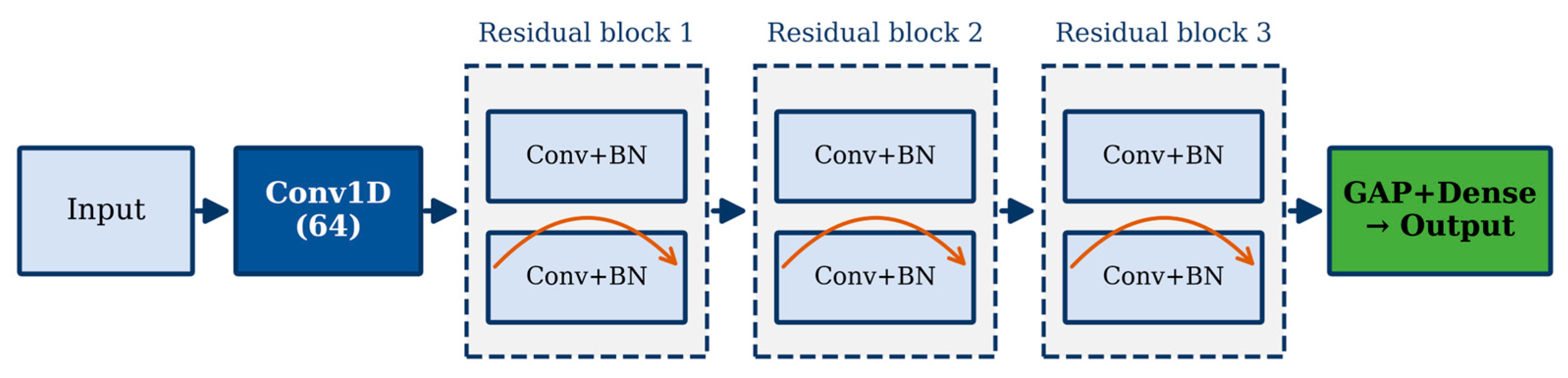
Four standalone ResNet variants were implemented to isolate the effects of optimizer and activation choice, forming a complete 2 × 2 factorial design: ResNet+SGD+ReLU, ResNet+SGD+Tanh, ResNet+Adam+ReLU, and ResNet+Adam+Tanh. All models share an identical backbone structure: one initial Conv1D layer followed by three residual blocks. The ResNet architecture is shown in Figure 5. Each block contains two Conv1D layers (kernel size 3, same padding), each followed by Batch normalization, with a skip connection adding the block input to its output [18,27]. The residual mapping is given as follows:

$$H\left(x\right)=F\left(x\right)+x$$

(13)

$$F\left(x\right)=W_2·BN\left(ReLU\left(W_1·BN\left(x\right)\right)\right)$$

(14)

where, in (13) and (14), H(x) is the desired mapping, F(x) is the learned residual, $x$ is the skip input, and BN denotes batch normalization [18]. The total convolutional depth is seven layers. Batch normalization is defined as follows:

$${\widehat{x}}_i={\displaystyle \frac{x_i - {\mu }_B}{\sqrt{{\sigma }_B^2+\epsilon }}}$$

(15)

$$y_i=\gamma ·{\widehat{x}}_i+\beta$$

(16)

where, in (15) and (16), the batch mean ${\mu }_B$ and variance ${\sigma }_B$ normalize each activation. The learnable scale and shift parameters restore representational capacity. A small constant $\epsilon$ ensures numerical stability [18].

3.5.3. Hybrid ResNet+LSTM and ResNet+GRU Models

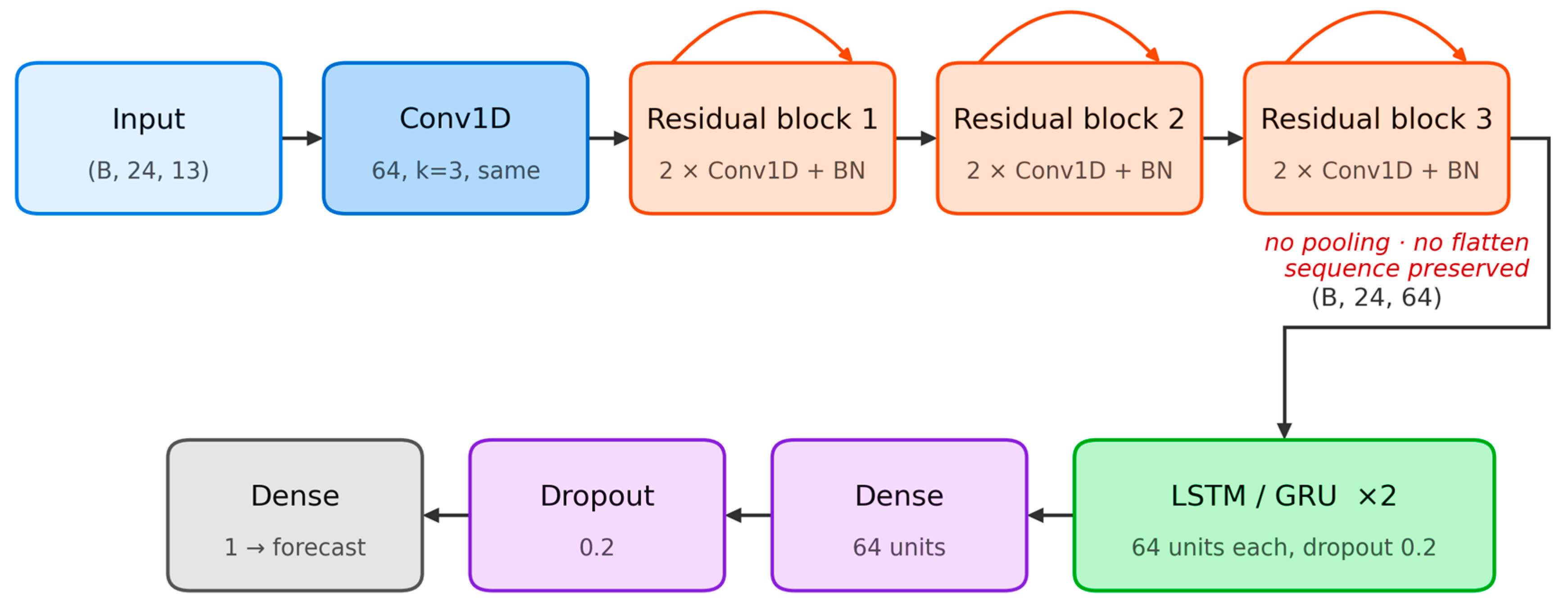
For the study of hybrid models, ResNet comprising seven convolutional layers and three residual blocks was used as the backbone to extract local temporal features and hierarchical patterns. The architecture of the hybrid model is given in Figure 6. Every convolutional layer uses 64 filters with kernel size 3 and same padding. Each residual block employs an identity shortcut with the activation applied after the addition. No striding, flattening, or pooling is applied at any point to preserve the temporal dimension, and the backbone output enters the recurrent stage as a (batch, 24, 64) sequence. This distinguishes the hybrids from the standalone ResNet variants, which reduce the sequence by global average pooling before their output layer.

Its output was then fed into two stacked recurrent layers, LSTM (or GRU), having 64 units each and a dropout rate of 0.2, with the first returning full sequences, and the second a single context vector to capture long-range sequential dependencies. The output head comprises a dense layer of 64 units, a dropout layer and a single-unit dense layer producing the forecast, providing a total of three dropout layers. This methodology combines local feature extraction with temporal memory, as proposed in [1,19,20,28].

3.5.4. Transformer Model (PatchTST)

PatchTST is a transformer-based architecture, specifically developed for time series forecasting by considering the look-back sequence in patches instead of treating each step as a token [40]. It reduces sequence length and allows the attention mechanism to perform over local segments. A sample PatchTST architecture is shown in Figure 7. Each input patch is linearly projected into an embedding space and enriched with a positional encoding:

$$z_i = W_p·p_i + E_{pos,i}$$

(17)

where the i^th patch is projected by a shared embedding matrix and combined with its positional encoding. The embedded patches then pass through a multi-head self-attention encoder:

$$Attention\left(Q,K,V\right)=softmax\left({\displaystyle \frac{Q Kᵀ}{\sqrt{d_k}}}\right)·V$$

(18)

where, in (18), Q, K, and V are the query, key, and value projections. $d_k$ is the key dimension [21]. A final linear head maps the encoded representation to the next-step load demand prediction. The model uses GELU activations and 0.2 dropout.

3.5.5. Optimizer Configuration

For SGD-optimized models, parameters are updated directly along the negative gradient using a single global learning rate:

$${\theta }_t={\theta }_{t-1}-\alpha g_t$$

(19)

where, in (19), $g_t$ is the gradient of the loss with respect to the parameters, and α is the learning rate. The same step size is applied to every parameter.

For Adam-optimized models, adaptive updates are computed from first and second moment estimates of the gradient:

$$m_t={\beta }_1{m}_{t-1}+\left(1-{\beta }_1\right)g_t$$

(20)

$$v_t={\beta }_2{v}_{t-1}+\left(1-{\beta }_2\right)g_t^2$$

(21)

which are bias-corrected:

$$m{̂}_t={\displaystyle \frac{m_t}{1 - {{\beta }_1}^{\mathrm{t}}}}$$

(22)

$${̂}_t={\displaystyle \frac{v_t}{1-{{\beta }_2}^{\mathrm{t}}}}$$

(23)

and applied as follows:

$${\theta }_t = {\theta }_{t-1} - \alpha ·{\displaystyle \frac{m{̂}_t}{\sqrt{v{̂}_t} + \epsilon }}$$

(24)

where the decay rates are ${\beta }_1$ = 0.9 and ${\beta }_2$ = 0.999. The stability constant is $\epsilon$ = 10⁻⁸. Unlike the uniform update rule in (19), the scheme in (20)–(24) adapts the effective learning rate for each parameter, which generally enables faster and more stable convergence [41].

In this study, the same learning rate (α = 0.001) was used by both optimizers. Gradient clipping by norm with a threshold of 1.0 was applied during all training runs. SGD was employed in its plain form without momentum. The selected learning rate is standard for Adam, but relatively small for plain SGD. Due to which, SGD generally requires a larger step size or momentum to achieve convergence at a similar rate. This configuration is retained intentionally as part of the controlled design: by keeping the learning rate constant, the effect of the optimization algorithm is isolated, and the resulting optimization shortfall of the SGD-trained models, consistent with incomplete convergence within the fixed epoch budget, is examined in Section 5.2.

3.6. Evaluation Metrics

Model performance was evaluated using four standard error metrics [1,4,12,30]. The mean absolute percentage error (MAPE) provides a scale-independent measure:

$$MAPE={\displaystyle \frac{100}{N}}\Sigma \left|{\displaystyle \frac{y_i-{\hat{\mathrm{y}}}_i}{y_i}}\right|$$

(25)

The root mean square error (RMSE) penalizes larger errors more heavily:

$$RMSE = \sqrt{{\displaystyle \frac{1}{N}}\Sigma {\left(y_i-{\hat{\mathrm{y}}}_i\right)}^2}$$

(26)

The mean absolute error (MAE) measures average error magnitude:

$$MAE={\displaystyle \frac{1}{N}}\Sigma \left|y_i-{\hat{\mathrm{y}}}_i\right|$$

(27)

where the actual ($y_i$) and predicted demand (${\hat{\mathrm{y}}}_i)$ values are compared across all $N$ test samples.

4. Case Study

4.1. Australian Electricity Demand Data

In this study, publicly available electricity demand data for the state of Queensland for the period 2006 to 2010 was obtained from the Australian Energy Market Operator (AEMO) [1]. The National Electricity Market of Australia poses distinctive forecasting challenges due to its climate variability and geographic diversity. These characteristics make it a demanding and widely used benchmark for load forecasting studies. The dataset comprises half-hourly electricity demand along with five corresponding related parameters, including dry-bulb temperature, dew-point temperature, wet-bulb temperature, humidity, and electricity price. In this way, it yields 48 values per day at half-hourly (thirty-minute) resolution, corresponding to approximately 87,600 time intervals for the five years. The dataset captures the characteristics of the daily cycles, weekly seasonality and annual trends of real electricity load demand and is widely used as a benchmark in previous demand forecasting studies [1,31,32], establishing its suitability for comparative model evaluation.

4.2. Training and Testing Configuration

A similar training configuration was used for all ten models to ensure a fair comparison. Each model was trained for 20 epochs using a batch size of 32, with gradient clipping by norm at a threshold of 1.0. MSE was used as the loss function. The test partition was supplied only for validation during training. It was used to monitor the model’s performance. Neither early stopping nor checkpoint selection was used to ensure that the monitored loss did not affect the model weights. The final models were taken after completing the fixed training budget. The data was split chronologically into 80% training and 20% testing to preserve the sequence of observations. Every model was trained using six independent random seeds: 42, 7, 123, 2024, 5 and 99. This approach was adopted for assessment of variability in training runs, arising due to the stochastic nature of neural-network training. All reported metrics are presented as the mean along with the sample standard deviation across the six seeds. Keeping the uniform protocol ensured that the difference in observed performance is attributable to model architecture and training configuration and not due to incidental variation in the training procedure [1,30].

The identical training budget was selected deliberately to ensure fair comparison, even though this may prevent some models from reaching their best performance. Results therefore describe models at a common budget rather than at their respective optima.

4.3. Evaluation Configuration

The trained models were evaluated under two regimes as defined in Section 3.1. The first regime is one-step-ahead testing over the full 2010 test year, comprising 17,472 rolling windows from 2 January to 31 December 2010. The performance of each model was evaluated by rolling one-step forecasting, in which the model predicts each next half-hourly value using an initial 12 h look-back window, constructed using the preceding actual historical data.

The second regime is multi-horizon evaluation. In this regime, recursive forecasts were generated up to 168 h from each daily midnight origin across the 2010 test year, resulting in 358 origins in total. The forecast errors were computed cumulatively at time horizons of 24 h, 48 h, and 168 h. The full test year is used because a claim related to long-horizon stability requires many rollouts. A single week at a 168 h horizon provides only one forecast trajectory, which is not enough to calculate a mean or a dispersion. To confirm that this asymmetry does not affect the reported ordering, both regimes were additionally evaluated on the alternative window. One-step error was computed over the full common span of 17,472 windows from 2 January to 31 December 2010. Employing the two forecasting regimes provides a comprehensive comparison of the models, both for one-step prediction accuracy and recursive multi-horizon forecasting performance.

5. Results and Discussion

5.1. Forecasting Results

As described in Section 4.3, each model was evaluated in two different ways. The one-step test forecasts only the next half-hour and then moves forward using the actual historical values. It is a widely adopted approach for evaluating load-forecasting models, providing a benchmark against previous studies. The other regime is multi-horizon forecasting, which is the primary focus of this study. Each model recursively generates forecasts up to 168 h ahead using the 358 daily midnight origins in the 2010 test year. At each forecasting step, the predicted load value is fed back into the input sequence to predict the load demand of the next time interval. The actual recorded values of other variables, i.e., weather, price, and calendar features, are provided. Forecast errors were computed cumulatively at time horizons of 24, 48, and 168 h. The experiment was repeated over six independent random seeds, and the average results were taken.

5.1.1. One-Step Forecasting Results

Table 2. One-step-forecasting errors (mean ± sample standard deviation) for test year 2010 over 6 random seeds.

Model	MAPE	RMSE	MAE
BiLSTM	0.80 ± 0.07	92.3 ± 8.7	70.4 ± 6.6
LSTM	0.81 ± 0.12	91.5 ± 8.8	69.9 ± 8.5
GRU	0.87 ± 0.15	95.8 ± 12.1	75.0 ± 11.8
PatchTST	0.94 ± 0.17	104.0 ± 13.2	81.6 ± 13.4
ResNet+Adam+Tanh	1.02 ± 0.14	111.6 ± 13.7	87.4 ± 11.5
ResNet+GRU	1.11 ± 0.22	118.9 ± 19.6	93.4 ± 16.1
ResNet+LSTM	1.18 ± 0.36	124.2 ± 29.1	99.9 ± 27.9
ResNet+Adam+ReLU	1.36 ± 0.18	139.5 ± 16.9	114.2 ± 16.7
ResNet+SGD+Tanh	4.65 ± 0.35	518.6 ± 36.1	399.9 ± 29.0
ResNet+SGD+ReLU	5.94 ± 0.33	647.2 ± 29.5	502.8 ± 26.0

provides the results of one-step MAPE, RMSE and MAE across the year 2010 (2 January–31 December). The recurrent models lead. BiLSTM is the most accurate over the full year with a mean MAPE of 0.80%, followed by LSTM (0.81%) and GRU (0.87%). PatchTST follows at 0.94% and then ResNet+Adam+Tanh (1.02%). Both hybrid models follow closely (1.11% and 1.18%). ResNet+Adam+Relu achieved 1.36%. The two SGD-trained ResNets performed worst with MAPE values of 4.65% and 5.94%. Their lower performance is consistent with incomplete convergence under the 20-epoch training budget. A similar pattern, with slight variations in ranking, can be observed for RMSE and MAE.

5.1.2. Multi-Horizon Forecasting Results

Table 3. Multi-step forecasting errors (mean ± sample standard deviation) for 24 h for the test year 2010 over 6 random seeds.

Model	24 h MAPE	24 h RMSE	24 h MAE
ResNet+SGD+ReLU	7.39 ± 0.21	754 ± 15	641 ± 16
ResNet+SGD+Tanh	8.39 ± 0.38	875 ± 37	737 ± 31
PatchTST	7.24 ± 2.08	803 ± 243	654 ± 189
LSTM	6.65 ± 2.33	739 ± 269	599 ± 213
ResNet+GRU	8.07 ± 2.06	868 ± 227	710 ± 181
BiLSTM	6.02 ± 2.43	696 ± 297	550 ± 228
ResNet+Adam+ReLU	10.79 ± 2.42	1145 ± 304	940 ± 246
ResNet+LSTM	10.33 ± 3.65	1139 ± 420	928 ± 332
GRU	8.33 ± 5.54	916 ± 659	737 ± 500
ResNet+Adam+Tanh	9.16 ± 3.49	1015 ± 397	818 ± 327

,

Table 4. Multi-step forecasting errors (mean ± sample standard deviation) for 48 h for the test year 2010 over 6 random seeds.

Model	48 h MAPE	48 h RMSE	48 h MAE
ResNet+SGD+ReLU	7.59 ± 0.20	787 ± 15	656 ± 15
ResNet+SGD+Tanh	8.74 ± 0.58	927 ± 61	763 ± 47
PatchTST	8.16 ± 2.46	894 ± 272	731 ± 221
LSTM	8.06 ± 3.29	886 ± 358	720 ± 298
ResNet+GRU	9.38 ± 2.69	1002 ± 279	817 ± 229
BiLSTM	7.77 ± 3.62	879 ± 406	697 ± 327
ResNet+Adam+ReLU	11.82 ± 2.56	1252 ± 310	1017 ± 253
ResNet+LSTM	12.62 ± 4.71	1365 ± 517	1107 ± 407
GRU	11.00 ± 8.97	1155 ± 911	956 ± 772
ResNet+Adam+Tanh	12.00 ± 5.13	1307 ± 545	1048 ± 461

and

Table 5. Multi-step forecasting errors (mean ± sample standard deviation) for 168 h for the test year 2010 over 6 random seeds.

Model	168 h MAPE	168 h RMSE	168 h MAE
ResNet+SGD+ReLU	7.81 ± 0.18	832 ± 19	673 ± 15
ResNet+SGD+Tanh	9.05 ± 0.77	985 ± 84	785 ± 62
PatchTST	9.20 ± 2.95	1008 ± 313	820 ± 262
LSTM	9.87 ± 4.51	1084 ± 474	879 ± 408
ResNet+GRU	10.40 ± 3.24	1119 ± 316	899 ± 266
BiLSTM	11.20 ± 6.54	1236 ± 656	987 ± 552
ResNet+Adam+ReLU	12.58 ± 2.80	1339 ± 329	1077 ± 280
ResNet+LSTM	13.99 ± 5.44	1533 ± 583	1211 ± 455
GRU	14.28 ± 12.49	1483 ± 1211	1249 ± 1092
ResNet+Adam+Tanh	14.76 ± 6.02	1588 ± 598	1272 ± 528

present the results of multi-horizon forecasting for 24 h, 48 h and 168 h, respectively. These results show a different performance trend. As the forecasting horizon increases, the relative ranking of the models changes substantively.

At the 24 h horizon, BiLSTM is still best with the lowest MAPE value of 6.02%, followed by LSTM at 6.65%. PatchTST ranks 3rd at 7.24%, and ResNet+SGD+ReLU ranks 4th at 7.39%, which was the lowest in one-step results. At a 48 h time horizon, ResNet+SGD+ReLU moved to 1st at 7.59%. At 168 h, two SGD-trained ResNets occupy the top two positions with MAPE values of 7.81% and 9.05%.

When the time horizon changes from 24 h to 168 h, BiLSTM moved from 6.02% to 11.20%, dropping its rank from 1st to 6th. Meanwhile, GRU moved from 8.33% to 14.28%, and ResNet+Adam+Tanh, which was mid-table at one step, showed the highest error of 14.76% for the 168 h time horizon. LSTM, which previously achieved the 2nd rank in one-step performance evaluation, finished 4th at 9.87%. PatchTST is 3rd at 168 h at 9.20% but does not lead at any horizon.

Two key observations emerge. First, the SGD-trained ResNets with ReLU and Tanh activation functions achieve the highest accuracy at 168 h. They also exhibit the greatest stability with standard deviations of 0.18 and 0.77 at 168 h. Second, the models that lead at 24 h are not those that lead at 168 h. However, the ranking is almost consistent across different evaluation metrics. At the time horizon of 168 h, the ordering based on RMSE and MAE matches that based on MAPE for the leading models, confirming that the observed ranking is usually not an artefact of the percentage-based metric.

Table 6. Model ranking by MAPE at different forecasting horizons.

	One-Step		24 h		48 h		168 h		Rank Variation from One Step to 168 h
Model	MAPE	Rank	MAPE	Rank	MAPE	Rank	MAPE	Rank
BiLSTM	0.80 ± 0.07	1	6.02 ± 2.43	1	7.77 ± 3.62	2	11.20 ± 6.54	6	−5
LSTM	0.81 ± 0.12	2	6.65 ± 2.33	2	8.06 ± 3.29	3	9.87 ± 4.51	4	−2
GRU	0.87 ± 0.15	3	8.33 ± 5.54	6	11.00 ± 8.97	7	14.28 ± 12.49	9	−6
PatchTST	0.94 ± 0.17	4	7.24 ± 2.08	3	8.16 ± 2.46	4	9.20 ± 2.95	3	+1
ResNet+Adam+Tanh	1.02 ± 0.14	5	9.16 ± 3.49	8	12.00 ± 5.13	9	14.76 ± 6.02	10	−5
ResNet+GRU	1.11 ± 0.22	6	8.07 ± 2.06	5	9.38 ± 2.69	6	10.40 ± 3.24	5	+1
ResNet+LSTM	1.18 ± 0.36	7	10.33 ± 3.65	9	12.62 ± 4.71	10	13.99 ± 5.44	8	−1
ResNet+Adam+ReLU	1.35 ± 0.18	8	10.79 ± 2.42	10	11.82 ± 2.56	8	12.58 ± 2.80	7	+1
ResNet+SGD+Tanh	4.64 ± 0.35	9	8.39 ± 0.38	7	8.74 ± 0.58	5	9.05 ± 0.77	2	+7
ResNet+SGD+ReLU	5.94 ± 0.33	10	7.39 ± 0.21	4	7.59 ± 0.20	1	7.81 ± 0.18	1	+9

summarizes the model rankings at each forecast horizon. Here, all ranks are computed over the full common span of the 2010 test year. This ensures that all models are compared over identical data. The two SGD-trained ResNets improve greatly and move from 10th and 9th at one step to 1st and 2nd at 168 h. GRU falls from 3rd to 9th and BiLSTM from 1st to 6th. Four models improve their rank with horizon, and five models become worse. Only ResNet+LSTM shows almost no change in rank. Figure 8 represents the same reversal as a rank trajectory.

5.2. Causes of Ranking Changes with Horizon

The observed change in performance ranking can be explained by a clear and consistent underlying mechanism. In the multi-horizon test, each model is fed its own predictions. Error rises over roughly the first 24 h, and then settles at a level characteristic of each model. The recurrent models settle at a higher level, whereas the SGD ResNets settle lower and overtake them at about 24 h.

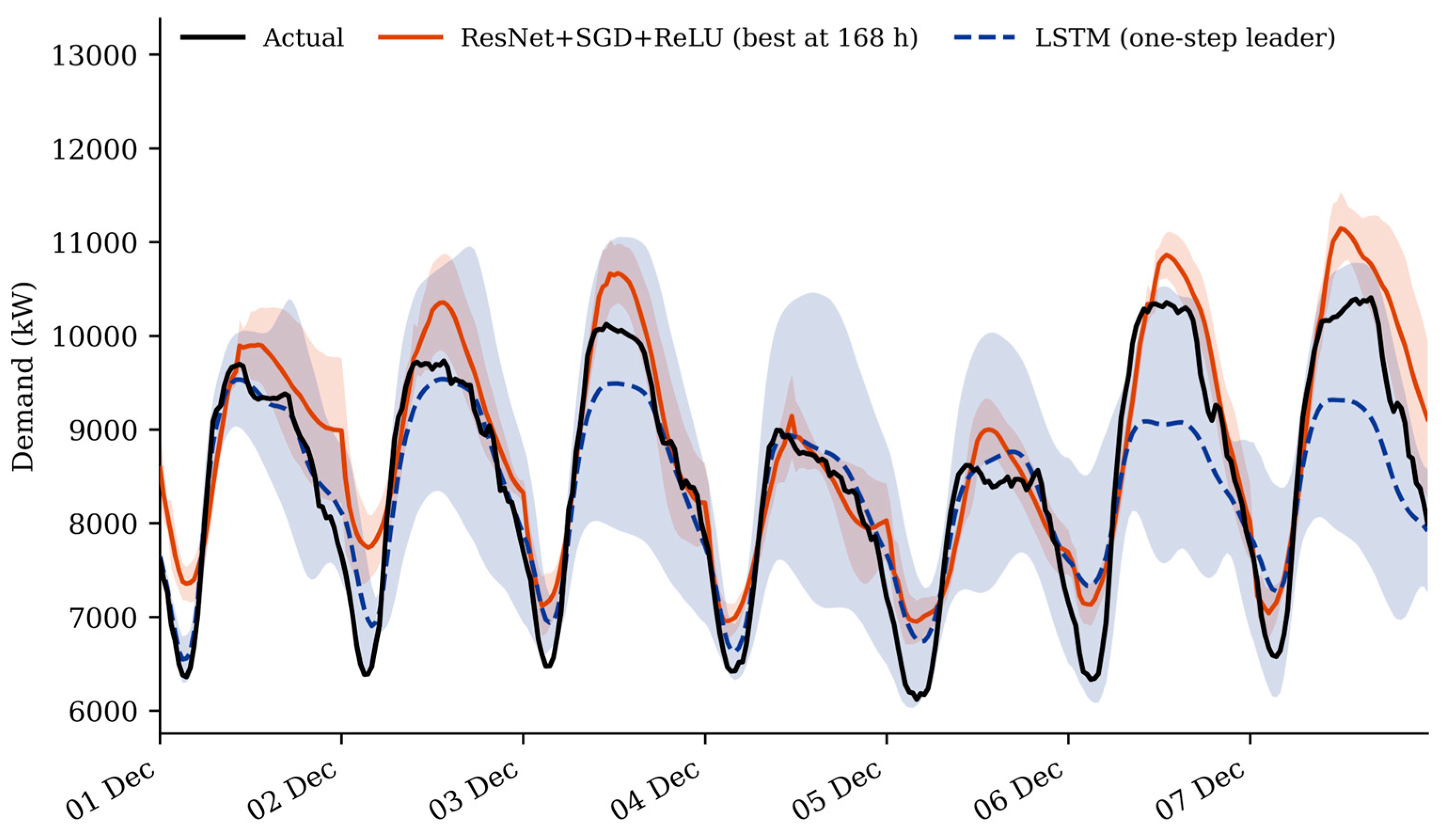
The SGD-trained ResNets had a mean training loss at epoch 20 of 0.0093 and 0.0073, against 0.0002 to 0.0011 for every other model, and were still descending. Their error settles at a lower plateau. This weakness at one step becomes a strength under long rollout, because a stable predictor settles at a lower error level once the rollout stabilizes. The very low seed-to-seed variation in the SGD-ResNets at long horizons supports this. They fail gracefully and repeatably, whereas the sharper models diverge unpredictably. Figure 9 shows it directly, where the lines are means over six random seeds. Shaded regions denote the span ± one standard deviation. The figure compares the best long-horizon model (ResNet+SGD+ReLU) with the one-step leader (LSTM) against the actual demand.

During the week, the ResNet+SGD+ReLU trajectory keeps the daily shape with a mean across-seed spread of 377 kW, overshooting some daily peaks rather than uniformly damping them. The LSTM trajectory, meanwhile, increasingly under-predicts the peaks, and its spread widens to 1041 kW.

This reframes the SGD “failure” reported in one-step studies—including Table 2—as horizon-specific rather than absolute. A model that performs poorly in one-step forecasting may nevertheless achieve superior performance over extended forecasting horizons, and vice versa. It also explains why added architectural complexity did not help: neither the ResNet hybrids nor the PatchTST transformer led at any horizon.

The consequence is clear. On this benchmark, selecting a model solely on the basis of one-step forecasting accuracy may select models that settle at the highest error levels over the longer forecasting horizons. This highlights the importance of horizon-aware evaluation.

5.3. Comparison of Results with Previous Studies

Table 7. One-step-ahead MAPE (mean ± sample standard deviation) for the three cumulative December 2010 test periods.

Model	1 December	1–2 December	1–7 December
LSTM	0.72 ± 0.13	0.76 ± 0.19	0.78 ± 0.17
BiLSTM	0.84 ± 0.09	0.80 ± 0.10	0.82 ± 0.13
GRU	0.82 ± 0.09	0.84 ± 0.12	0.86 ± 0.16
PatchTST	0.94 ± 0.29	0.92 ± 0.23	0.91 ± 0.19
ResNet+Adam+Tanh	0.93 ± 0.20	1.00 ± 0.25	0.99 ± 0.18
ResNet+GRU	1.03 ± 0.31	1.05 ± 0.28	1.06 ± 0.24
ResNet+LSTM	1.18 ± 0.37	1.22 ± 0.49	1.20 ± 0.45
ResNet+Adam+ReLU	1.41 ± 0.34	1.35 ± 0.26	1.39 ± 0.17
ResNet+SGD+Tanh	4.77 ± 1.32	5.06 ± 1.18	3.78 ± 0.51
ResNet+SGD+ReLU	6.24 ± 1.26	6.14 ± 0.67	4.89 ± 0.41

and

Table 8. Multi-step-ahead MAPE (mean ± sample standard deviation) for the 1–7 December 2010 test periods.

Model	24 h	48 h	168 h
ResNet+SGD+ReLU	6.286 ± 0.949	6.385 ± 0.878	6.436 ± 1.131
ResNet+SGD+Tanh	6.818 ± 0.585	7.156 ± 0.488	7.751 ± 1.595
PatchTST	7.410 ± 3.318	8.194 ± 3.734	8.892 ± 4.214
LSTM	7.222 ± 3.636	8.441 ± 4.576	10.095 ± 5.926
ResNet+GRU	8.766 ± 4.616	10.724 ± 5.271	12.014 ± 6.111
BiLSTM	7.735 ± 4.104	9.619 ± 5.363	12.588 ± 7.043
ResNet+Adam+ReLU	11.721 ± 4.332	12.274 ± 3.382	12.956 ± 2.931
GRU	8.738 ± 6.295	12.209 ± 12.162	15.293 ± 15.377
ResNet+LSTM	11.412 ± 5.592	13.861 ± 5.672	16.940 ± 6.206
ResNet+Adam+Tanh	10.693 ± 5.441	13.854 ± 7.260	17.044 ± 8.923

present the MAPE results of one-step and multi-step forecasting obtained in this study. For one-step forecasting, the three cumulative periods used are the same as those chosen by the closest comparable study by Chen et al. [1], which evaluated a ResNet–LSTM hybrid on the same Queensland dataset. The best reported MAPE result for the period of 1–7 December test period by [1] is approximately 0.597% and was obtained by the ResNet–LSTM hybrid using one-step-ahead evaluation. On the basis of these results, they concluded that the ResNet-LSTM hybrid model outperformed the other architectures considered.

As compared to [1], the one-step results of the present study are of a likewise low order, with LSTM producing a MAPE of 0.78% and BiLSTM 0.82% over the same 1–7 December window. It is therefore confirmed that the proposed evaluation pipeline produces competitive one-step forecasting results on the identical dataset.

However, the objective of the present study is different and is not to identify the best-performing architecture under one-step evaluation. It compares ten models covering residual, recurrent, transformer and hybrid families under a common experimental protocol. Further, rather than limiting to one-step forecasting, the evaluation is extended to recursive multi-horizon forecasting at time horizons of 24, 48, and 168 h, which was not considered by Chen et al. [1]. From this point of view, both studies are complementary. Chen et al. [1] established that a hybrid ResNet–LSTM model achieves the best one-step forecasting accuracy, whereas the results in this study show that the model ranking changes considerably with increasing forecasting horizon. No single deep learning model performs best across all horizons. Specifically, the SGD-trained ResNet variants, which show the lowest accuracy under one-step evaluation in Table 7, rank 1st and 2nd among the ten models at the 168 h horizon in Table 8.

It is pertinent to highlight that the reported accuracy on a benchmark dataset can be influenced by many factors, such as look-back window length, data preprocessing, hyperparameter settings, and training budget. Reproducing a specific published error value is, therefore, not the primary objective of this study. Instead, the primary contribution of the present study is a controlled comparison of ten representative deep learning models under a consistent multi-horizon evaluation protocol.

As stated earlier, the objective of selecting the ten models was to ensure representation across four architectural families, rather than to identify the overall best-performing model. The PatchTST deep learning model was selected to represent the transformer family. It is one of the most widely adopted transformer models and is repeatedly used as a baseline model for comparison with newer architectures—such as iTransformer [42], TimesNet [43], and DLinear [44]. An independent benchmark of five transformer variants for energy forecasting found PatchTST to be the most accurate of the group [45]. It therefore provides a strong and representative modern baseline, without claiming to be the newest or best possible design.

The results also contribute to the ongoing discussion regarding the value of increased architectural complexity. A growing body of work questions whether elaborate convolutional, residual, and attention-based models consistently outperform simpler baselines [7,30], with several recent studies finding that lightweight or linear models rival transformers on standard benchmarks [44]. The observation that neither the ResNet-based hybrid models nor PatchTST outperforms the simpler models at any forecasting horizon is consistent with this perspective.

6. Conclusions

This paper presented a controlled comparative evaluation of ten deep learning models for short-term electricity demand forecasting on publicly available Queensland, Australia data (2006–2010). Ten deep learning models, including recurrent models (LSTM, GRU, BiLSTM), residual models (four ResNet variants forming a complete optimizer × activation design), hybrid models (ResNet+LSTM, ResNet+GRU) and a transformer model (PatchTST), were trained. The same preprocessing pipeline, identical dataset, data splits, and training budget were used for all models to isolate the effect of training configuration and model architecture. Each model was evaluated under two forecasting regimes: rolling one-step-ahead and recursive multi-horizon forecasting at time horizons of 24 h, 48 h, and 168 h, rolled out from 358 daily origins across the 2010 test year. Results were reported as the mean and standard deviation over six random seeds. Under one-step evaluation for the complete year 2010, the recurrent models achieved the best performance. BiLSTM recorded the lowest MAPE of 0.80%, whereas the SGD-trained ResNets produced the highest errors. As the horizon extended, this ranking reversed: at 168 h, the two SGD-trained ResNets ranked 1st and 2nd among the ten evaluated models and were by far the most stable models across seeds, while the BiLSTM, a leader at one step, fell to 6th rank. The more complex PatchTST transformer did not lead at any horizon.

Three main conclusions can be drawn from the results. First, the best model depends on the forecast horizon. Second, one-step accuracy does not transfer to multi-step performance on this benchmark, so models must be evaluated at the horizon they will actually be used for. Third, added architectural complexity may not improve accuracy at any horizon—neither the ResNet hybrids nor the PatchTST transformer led at any horizon.

This study has several limitations that suggest directions for future research. The evaluation used a single dataset from one region; assessment on additional datasets from different climates and markets would strengthen generalizability. The multi-horizon forecasts assume that future weather, price, and calendar values are available, isolating demand-forecasting behavior from the separate problem of weather forecasting; relaxing this assumption is a natural extension. The configuration used in this study was fixed by design rather than optimized. In the future, the impact of hyperparameter tuning on ranking reversal can be studied. Similarly, the impact of the look-back window, longer time horizons, etc. on the ranking of various models can be examined in future works.

References

1. Chen, X.; Chen, W.; Dinavahi, V.; Liu, Y.; Feng, J. Short-term load forecasting and associated weather variables prediction using ResNet-LSTM based deep learning. IEEE Access 2023, 11, 5393–5405. [Google Scholar] [CrossRef] [Scilit]
2. Özen, S.; Yazıcı, A.; Atalay, V. Hybrid deep learning models with data fusion approach for electricity load forecasting. Expert Syst. 2025, 42, e13741. [Google Scholar] [CrossRef] [Scilit]
3. Asiri, M.M.; Aldehim, G.; Alotaibi, F.A.; Alnfiai, M.M.; Assiri, M.; Mahmud, A. Short-term load forecasting in smart grids using hybrid deep learning. IEEE Access 2024, 12, 23504–23513. [Google Scholar] [CrossRef] [Scilit]
4. Al Mamun, A.; Sohel, M.; Mohammad, N.; Sunny, M.S.H.; Dipta, D.R.; Hossain, E. A comprehensive review of the load forecasting techniques using single and hybrid predictive models. IEEE Access 2020, 8, 134911–134939. [Google Scholar] [CrossRef] [Scilit]
5. Ullah, K.; Ahsan, M.; Hasanat, S.M.; Haris, M.; Yousaf, H.; Raza, S.F.; Tandon, R.; Abid, S.; Ullah, Z. Short-term load forecasting: A comprehensive review and simulation study with CNN-LSTM hybrids approach. IEEE Access 2024, 12, 111858–111881. [Google Scholar] [CrossRef] [Scilit]
6. Chakhchoukh, Y.; Panciatici, P.; Mili, L. Electric load forecasting based on statistical robust methods. IEEE Trans. Power Syst. 2010, 26, 982–991. [Google Scholar] [CrossRef] [Scilit]
7. Akhtar, S.; Shahzad, S.; Zaheer, A.; Ullah, H.S.; Kilic, H.; Gono, R.; Jasiński, M.; Leonowicz, Z. Short-term load forecasting models: A review of challenges, progress, and the road ahead. Energies 2023, 16, 4060. [Google Scholar] [CrossRef] [Scilit]
8. Shaikh, M.S.; Lin, H.; Xie, S.; Dong, X.; Lin, Y.; Shiva, C.K.; Mbasso, W.F. An intelligent hybrid grey wolf-particle swarm optimizer for optimization in complex engineering design problem. Sci. Rep. 2025, 15, 18313. [Google Scholar] [CrossRef] [Scilit] [PubMed]
9. Shaikh, M.S.; Raj, S.; Babu, R.; Kumar, S.; Sagrolikar, K. A hybrid moth–flame algorithm with particle swarm optimization with application in power transmission and distribution. Decis. Anal. J. 2023, 6, 100182. [Google Scholar] [CrossRef] [Scilit]
10. Akarne, Y.; Essadki, A.; Nasser, T.; Annoukoubi, M. Enhanced smart microgrid scheduling: An empirical study on simultaneous energy supply and demand optimization using binary sparrow search algorithm. Results Eng. 2025, 27, 106811. [Google Scholar] [CrossRef] [Scilit]
11. Hochreiter, S.; Schmidhuber, J. Long short-term memory. Neural Comput. 1997, 9, 1735–1780. [Google Scholar] [CrossRef] [Scilit] [PubMed]
12. Torres, J.F.; Martinez-Alvarez, F.; Troncoso, A. A deep LSTM network for the Spanish electricity consumption forecasting. Neural Comput. Appl. 2022, 34, 10533–10545. [Google Scholar] [CrossRef] [Scilit] [PubMed]
13. Kong, W.; Dong, Z.Y.; Jia, Y.; Hill, D.J.; Xu, Y.; Zhang, Y. Short-term residential load forecasting based on LSTM recurrent neural network. IEEE Trans. Smart Grid 2017, 10, 841–851. [Google Scholar] [CrossRef] [Scilit]
14. Vangipuram, S.R.; Giridhar, A. Short term residential load forecasting using temporal weather based embedding stacked LSTMs. IEEE Lat. Am. Trans. 2025, 23, 497–507. [Google Scholar] [CrossRef] [Scilit]
15. Kim, T.-Y.; Cho, S.-B. Predicting residential energy consumption using CNN-LSTM neural networks. Energy 2019, 182, 72–81. [Google Scholar] [CrossRef] [Scilit]
16. Zhang, S.; Chen, R.; Cao, J.; Tan, J. A CNN and LSTM-based multi-task learning architecture for short and medium-term electricity load forecasting. Electr. Power Syst. Res. 2023, 222, 109507. [Google Scholar] [CrossRef] [Scilit]
17. Wan, A.; Chang, Q.; Khalil, A.-B.; He, J. Short-term power load forecasting for combined heat and power using CNN-LSTM enhanced by attention mechanism. Energy 2023, 282, 128274. [Google Scholar] [CrossRef] [Scilit]
18. He, K.; Zhang, X.; Ren, S.; Sun, J. Deep residual learning for image recognition. In Proceedings of the 2016 IEEE Conference on Computer Vision and Pattern Recognition (CVPR); IEEE: New York, NY, USA, 2016; pp. 770–778. [Google Scholar]
19. Albelwi, S. A robust energy consumption forecasting model using ResNet-LSTM with huber loss. Int. J. Comput. Sci. Netw. Secur. 2022, 22, 301–307. [Google Scholar]
20. Sheng, Z.; An, Z.; Wang, H.; Chen, G.; Tian, K. Residual LSTM based short-term load forecasting. Appl. Soft Comput. 2023, 144, 110461. [Google Scholar] [CrossRef] [Scilit]
21. Vaswani, A.; Shazeer, N.; Parmar, N.; Uszkoreit, J.; Jones, L.; Gomez, A.N.; Kaiser, Ł.; Polosukhin, I. Attention is all you need. Adv. Neural Inf. Process. Syst. 2017, 30. [Google Scholar]
22. Pentsos, V.; Tragoudas, S.; Wibbenmeyer, J.; Khdeer, N. A hybrid LSTM-Transformer model for power load forecasting. IEEE Trans. Smart Grid 2025, 16, 2624–2634. [Google Scholar] [CrossRef] [Scilit]
23. Cho, K.; Van Merriënboer, B.; Gulçehre, Ç.; Bahdanau, D.; Bougares, F.; Schwenk, H.; Bengio, Y. Learning phrase representations using RNN encoder–decoder for statistical machine translation. In Proceedings of the 2014 Conference on Empirical Methods in Natural Language Processing (EMNLP), Doha, Qatar, 25–29 October 2014; pp. 1724–1734. [Google Scholar]
24. Sekhar, C.; Dahiya, R. Robust framework based on hybrid deep learning approach for short term load forecasting of building electricity demand. Energy 2023, 268, 126660. [Google Scholar] [CrossRef] [Scilit]
25. Goh, H.H.; He, B.; Liu, H.; Zhang, D.; Dai, W.; Kurniawan, T.A.; Goh, K.C. Multi-convolution feature extraction and recurrent neural network dependent model for short-term load forecasting. IEEE Access 2021, 9, 118528–118540. [Google Scholar] [CrossRef] [Scilit]
26. Dewangan, F.; Biswal, M.; Kishor, N. A Methodology for Electricity Demand Forecasting Using a Hybrid Approach. IEEE Access 2025, 13, 112197–112214. [Google Scholar] [CrossRef] [Scilit]
27. He, K.; Zhang, X.; Ren, S.; Sun, J. Identity mappings in deep residual networks. In Proceedings of the European Conference on Computer Vision; Springer: Cham, Switzerland, 2016; pp. 630–645. [Google Scholar]
28. Chen, K.; Chen, K.; Wang, Q.; He, Z.; Hu, J.; He, J. Short-term load forecasting with deep residual networks. IEEE Trans. Smart Grid 2018, 10, 3943–3952. [Google Scholar] [CrossRef] [Scilit]
29. Mirza, A.F.; Mansoor, M.; Usman, M.; Ling, Q. Hybrid Inception-embedded deep neural network ResNet for short and medium-term PV-Wind forecasting. Energy Convers. Manag. 2023, 294, 117574. [Google Scholar] [CrossRef] [Scilit]
30. Jang, J.; Kim, B.; Kim, I. Comparative analysis of deep learning techniques for load forecasting in power systems using single-layer and hybrid models. Int. Trans. Electr. Energy Syst. 2024, 2024, 5587728. [Google Scholar] [CrossRef] [Scilit]
31. Singh, N.K.; Singh, A.K.; Paliwal, N. Neural Network based short-term electricity demand forecast for Australian states. In Proceedings of the 2016 IEEE 1st International Conference on Power Electronics, Intelligent Control and Energy Systems (ICPEICES); IEEE: New York, NY, USA, 2016; pp. 1–4. [Google Scholar]
32. Al Khafaf, N.; Jalili, M.; Sokolowski, P. Application of deep learning long short-term memory in energy demand forecasting. In Proceedings of the International Conference on Engineering Applications of Neural Networks; Springer International Publishing: Cham, Switzerland, 2019; pp. 31–42. [Google Scholar]
33. Ben Taieb, S.; Atiya, A.F. A Bias and Variance Analysis for Multistep-Ahead Time Series Forecasting. IEEE Trans. Neural Netw. Learn. Syst. 2016, 27, 62–76. [Google Scholar] [CrossRef] [Scilit] [PubMed]
34. Taieb, S.B.; Bontempi, G.; Atiya, A.F.; Sorjamaa, A. A review and comparison of strategies for multi-step ahead time series forecasting based on the NN5 forecasting competition. Expert Syst. Appl. 2012, 39, 7067–7083. [Google Scholar] [CrossRef] [Scilit]
35. Marcellino, M.; Stock, J.H.; Watson, M.W. A comparison of direct and iterated multistep AR methods for forecasting macroeconomic time series. J. Econom. 2006, 135, 499–526. [Google Scholar] [CrossRef] [Scilit]
36. Masum, S.; Liu, Y.; Chiverton, J. Multi-step time series forecasting of electric load using machine learning models. In Proceedings of the International Conference on Artificial Intelligence and Soft Computing; Springer International Publishing: Cham, Switzerland, 2018; pp. 148–159. [Google Scholar]
37. Sehovac, L.; Grolinger, K. Deep learning for load forecasting: Sequence to sequence recurrent neural networks with attention. IEEE Access 2020, 8, 36411–36426. [Google Scholar] [CrossRef] [Scilit]
38. Morais, L.B.S.; Aquila, G.; de Faria, V.A.D.; Lima, L.M.M.; Lima, J.W.M.; de Queiroz, A.R. Short-term load forecasting using neural networks and global climate models: An application to a large-scale electrical power system. Appl. Energy 2023, 348, 121439. [Google Scholar] [CrossRef] [Scilit]
39. Qureshi, M.; Arbab, M.A.; Rehman, S.U. Deep learning-based forecasting of electricity consumption. Sci. Rep. 2024, 14, 6489. [Google Scholar] [CrossRef] [Scilit] [PubMed]
40. Nie, Y.; Nguyen, N.H.; Sinthong, P.; Kalagnanam, J. A time series is worth 64 words: Long-term forecasting with transformers. In Proceedings of the International Conference on Learning Representations (ICLR), Kigali, Rwanda, 1–5 May 2023. [Google Scholar]
41. Kingma, D.P.; Ba, J. Adam: A method for stochastic optimization. In Proceedings of the International Conference on Learning Representations (ICLR), San Diego, CA, USA, 7–9 May 2015. [Google Scholar]
42. Liu, Y.; Hu, T.; Zhang, H.; Wu, H.; Wang, S.; Ma, L.; Long, M. iTransformer: Inverted transformers are effective for time series forecasting. In Proceedings of the International Conference on Learning Representations (ICLR), Vienna, Austria, 7–11 May 2024. [Google Scholar]
43. Wu, H.; Hu, T.; Liu, Y.; Zhou, H.; Wang, J.; Long, M. TimesNet: Temporal 2D-variation modeling for general time series analysis. In Proceedings of the International Conference on Learning Representations (ICLR), Kigali, Rwanda, 1–5 May 2023. [Google Scholar]
44. Zeng, A.; Chen, M.; Zhang, L.; Xu, Q. Are transformers effective for time series forecasting? Proc. AAAI Conf. Artif. Intell. 2023, 37, 11121–11128. [Google Scholar] [CrossRef] [Scilit]
45. Suresh, V. Benchmarking transformer variants for hour-ahead PV forecasting: PatchTST with adaptive conformal inference. Energies 2025, 18, 5000. [Google Scholar] [CrossRef] [Scilit]
Figure 1. Input features and predicted one-step ahead demand of the forecasting models.
Electricity 07 00106 g001
Figure 2. Tensor-based window representation of the model input and output.
Electricity 07 00106 g002
Figure 3. Overall process flowchart of the study.
Electricity 07 00106 g003
Figure 4. Recurrent-model architecture, common to the LSTM, GRU, and bidirectional LSTM (two stacked recurrent layers of 64 units with dropout, followed by a dense output).
Electricity 07 00106 g004
Figure 5. Residual (ResNet) architecture: an initial convolution followed by three residual blocks, each with two convolutional layers, batch normalization, and a skip connection.
Electricity 07 00106 g005
Figure 6. Hybrid architecture (ResNet+LSTM/ResNet+GRU): the residual backbone extracts local features that are passed to stacked recurrent layers for temporal modeling. Three dropout layers in total: one after each recurrent layer and one in the output head.
Electricity 07 00106 g006
Figure 7. PatchTST architecture: the look-back sequence is split into patches, linearly embedded with positional encodings, processed by a multi-head self-attention encoder, and mapped to the next-step prediction by a linear head.
Electricity 07 00106 g007
Figure 8. Model ranking by MAPE at one step and at 24, 48, and 168 h, showing the reversal.
Electricity 07 00106 g008
Figure 9. Actual and predicted demand over the 168 h forecasting horizon from the 1 December 2010 origin. Shaded regions denote the span ± one standard deviation.
Electricity 07 00106 g009