Multi-Objective BESS Siting and Sizing via NSGA-II and PTDF-Constrained DC Optimal Power Flow: Application to the Mali Transmission Network

Abstract

Weak grid infrastructure and the absence of flexible storage are among the principal barriers to reliable, low-carbon energy access in sub-Saharan transmission systems. This paper proposes a hierarchical multi-objective framework for the optimal siting and sizing of battery energy storage systems (BESSs), applied to the 130-bus Mali transmission network within the EMERGE project. The upper level employs NSGA-II to simultaneously maximize daily price arbitrage revenue and minimize active power losses; the lower level solves a network-constrained DC optimal power flow with thermal branch limits enforced as hard linear inequalities via the Power Transfer Distribution Factor (PTDF) matrix. Over 500 generations, the framework identifies Bus 91 (SIRAKORO II, 150 kV) as the dominant storage location, achieving a maximum daily revenue of approximately €10,033 at a marginal loss increment of $6.7\times {10}^{-3}$ MWh. The resulting Pareto front gives Mali system planners a quantitative tool for trading off private investment returns against grid-level environmental impact, demonstrating that rigorous network-constrained BESS planning is technically tractable and economically viable in the resource-constrained context of sub-Saharan energy transitions.

1. Introduction

1.1. Motivation

The accelerating deployment of variable renewable energy sources—primarily solar photovoltaic and wind—creates increasingly severe temporal mismatches between generation and load that traditional dispatchable resources cannot resolve efficiently [1]. Large-scale battery energy storage systems (BESSs) have emerged as a key technology for bridging these gaps through price arbitrage, charging during low-price valley periods and discharging during high-price peak periods, thereby capturing the spread in spot market prices while contributing to system balance [2]. In emerging economies with weak grid infrastructure, such as the sub-Saharan networks targeted by the EMERGE project, this dual role—economic revenue generation and technical network support—is particularly relevant, since the transmission grid itself may constitute a binding constraint on how much arbitrage potential can be realized [3,4]. The interaction between battery injections and the physical network is therefore not a secondary consideration but a first-order determinant of both the economic value and the technical impact of any BESS installation. Indeed, as the African Development Bank’s Desert-to-Power initiative highlights for Mali, the expansion of renewable generation capacity must be matched by a commensurate investment in transmission infrastructure and flexible storage resources to enable effective energy evacuation and market participation [5].

A rigorous planning model must therefore integrate investment decisions—location, power rating, energy capacity—with operational constraints including state-of-charge dynamics, branch thermal limits, and generation balance, over a representative time horizon [6,7]. The resulting optimization is a mixed-integer nonlinear program (MINLP) whose size grows rapidly with network dimension and time resolution [8]. Direct solution approaches based on full AC optimal power flow are computationally prohibitive at the scale required by evolutionary algorithms: for a 500-generation NSGA-II run with a population of 30, a single AC power flow at every fitness evaluation would require more than $15\times {10}^6$ Newton–Raphson solve calls, each with $\mathcal{O}\left(n^3\right)$ complexity [9,10]. The linearized DC framework, combined with the pre-computed PTDF matrix and the vectorized EDCPF model, reduces this bottleneck to a sparse LU back-substitution per time step, making the full optimization tractable without abandoning the physics of power transfer distribution [11,12].

Multi-objective optimization for BESS siting and sizing has evolved along two parallel tracks. Early work focused on single-objective placement in distribution networks, using dynamic OPF or MILP formulations to minimize cost or energy losses [7,13]. A second wave introduced evolutionary multi-objective methods—primarily NSGA-II and NSGA-III—to capture the inherent trade-off between economic and technical objectives in distribution feeders, typically relying on simplified AC or penalty-based network models [14,15]. Transmission-level studies have addressed congestion and cost objectives using heuristic approaches on real national grids [8], but without a rigorous multi-objective framework. The combination of a multi-objective evolutionary search with exact, PTDF-embedded thermal constraints applied to a real sub-Saharan transmission network has not been previously reported.

Table 1 places the proposed framework in the context of recent BESS planning studies. The distinguishing features of this work are the combination of a multi-objective evolutionary search with a PTDF-constrained DC-OPF lower level applied to a real sub-Saharan transmission network.

Table 1. Comparison of selected BESS planning methods from the literature.

Reference	Algorithm	Test Network	Objectives	Network Model
Gill et al. [7]	Dynamic OPF	UK distribution	Cost, losses	AC OPF
López-Ramos et al. [13]	MILP	IEEE 14-bus	Revenue	DC, penalty
Avendaño [8]	Heuristic	Colombian grid	Cost, congestion	DC
Qin et al. [14]	NSGA-II	IEEE 33-bus	Cost, reliability	AC (simplified)
Su et al. [15]	NSGA-III	Distribution feeder	Cost, voltage	AC OPF
This work	NSGA-II + DC-OPF	Mali 130-bus	Revenue, losses	PTDF DC, EDCPF

Bold row: method proposed in this work, highlighted to distinguish it from the literature methods listed above.

1.2. Contributions

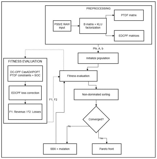
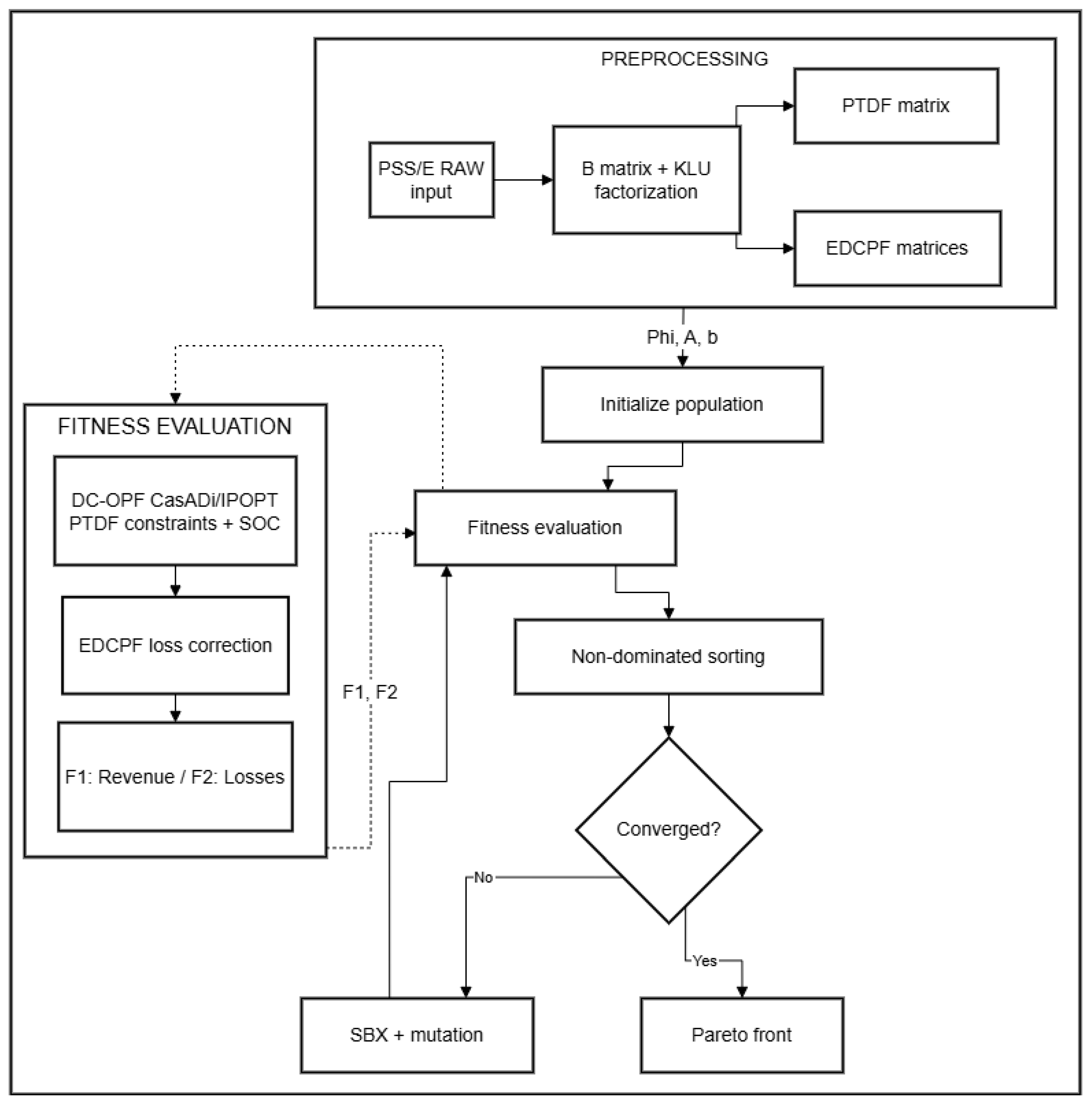
This work presents a hierarchical decomposition of the BESS planning MINLP that separates design decisions from operational ones while maintaining rigorous physical coupling between the two levels; the overall framework is summarized in Figure 1. Five specific contributions are identified:

Figure 1. Overall framework of the proposed multi-objective BESS planning methodology. The preprocessing block (top) assembles the susceptance matrix, computes the KLU factorization, and derives the PTDF and EDCPF matrices once before the evolutionary loop begins. The NSGA-II loop (center) drives the design-space search through non-dominated sorting and crowding distance selection. For each candidate, the fitness evaluation sub-block (right) solves the DC-OPF scheduling problem via CasADi/IPOPT with PTDF-embedded thermal constraints, then applies the EDCPF correction to recover voltage magnitudes and compute cycle losses. The two highlighted blocks correspond to the key innovations of the proposed framework.

• Four-gene chromosome formulation for the upper-level search. The NSGA-II evolutionary search [16] operates on chromosome encoding charging power, discharging power, energy capacity, and an installation bus simultaneously, implemented through PyGAD with non-dominated sorting and crowding distance selection—an approach shown to be well-suited for multi-objective BESS planning in distribution networks [14,15].
• PTDF-based thermal constraints as hard linear inequalities. Branch thermal limits are embedded directly inside the lower-level nonlinear program (NLP) solved by CasADi/IPOPT [17], ensuring that every candidate schedule is physically feasible on the transmission network without external penalty weighting—a critical improvement over penalty-based formulations [12,13].
• Vectorized EDCPF loss estimation layer. A vectorized extended DC power flow (EDCPF) layer [18] recovers voltage magnitudes from DC angles at negligible additional computational cost, enabling loss computation with sub-percent accuracy relative to a full AC solution [19].
• Transparent three-winding transformer handling via star-bus expansion. Five three-winding transformers (TR3Ws) in the PSS/E RAW network model are expanded into star-bus equivalents prior to matrix assembly, preserving admittance fidelity without introducing any special-case logic in the PTDF or OPF formulations.
• Cyclic state-of-charge constraint for single-day validity. Fixing both the initial and final state of charge (SOC) at $0.5·E_{\max }$ prevents horizon-end revenue inflation and makes single-day optimization results a valid proxy for steady-state multi-day operation [20].

The framework is validated on the real 130-bus Mali transmission network from the EMERGE project—a system representative of sub-Saharan infrastructure with limited meshing, multiple voltage levels (15 kV to 225 kV), and a small number of electrically dominant buses [21,22]. Experiment 3, comprising 500 NSGA-II generations and 55,890 stored Pareto front solutions across all generations, provides statistically robust evidence of convergence and demonstrates that the proposed framework produces actionable planning recommendations even for networks with challenging topological characteristics. The resulting Pareto front gives system operators a principled tool for balancing economic objectives against network technical constraints in the context of BESS investment planning [23,24].

2. Mathematical Methodology

2.1. Network Model and Susceptance Matrix

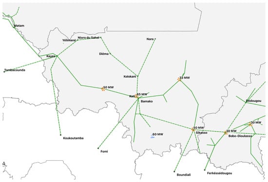
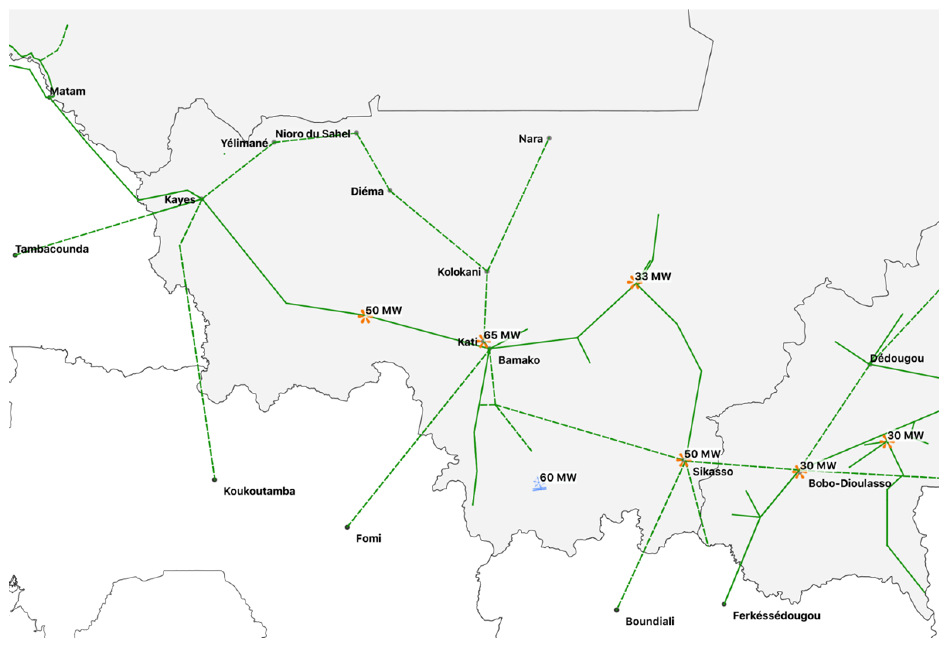
The mathematical foundation of the proposed framework rests on the DC linearization of the power flow equations, which transforms the nonlinear network model into a set of linear relations between bus angle differences and active power flows. Before this linearization can be applied, the network topology must be parsed and normalized into a form that is compatible with the nodal susceptance matrix assembly. For the Mali network, this pre-processing step is particularly important because the PSS/E RAW v33 file (grid_mali.raw) contains five three-winding transformers (TR3Ws) that cannot be represented as simple two-terminal elements in the standard DC model. Each TR3W is expanded into three two-winding branches meeting at a synthetic star bus whose index does not correspond to any physical bus in the network, but whose admittance equivalence is exact with respect to the port behavior seen from each physical winding. This expansion is performed in the parser layer, so the solver receives only standard two-terminal elements and assembles the susceptance matrix without any branching logic. The resulting network topology is illustrated in Figure 2.

Figure 2. High-voltage transmission network of Mali, showing the main 225 kV and 150 kV corridors connecting the principal generation centers to the Bamako load area. Bus 91 (SIRAKORO II, 150 kV)—the dominant BESS location identified by Experiment 3—is located at the electrically central node of the 150 kV subgraph. Adapted from Figure 6 of [5].

The nodal susceptance matrix $\mathbf{B}\in {\mathbb{R}}^{n\times n}$ is assembled by iterating over all active branches. For each branch $(i,j)$ with reactance $X_{ij}$ and status equal to 1:

$$B_{ij}-={\displaystyle \frac{1}{X_{ij}}},B_{ii}+={\displaystyle \frac{1}{X_{ij}}},B_{jj}+={\displaystyle \frac{1}{X_{ij}}}.$$

(1)

Branches with $|X_{ij}|<{10}^{-10}$ p.u. are skipped to avoid numerical singularity. Once assembled, the matrix is passed to CasADi as a ca.DM sparse object, and the reduced system ${\mathbf{B}}_{red}$ (obtained by removing the slack bus row and column) is factorized once via the Clark–Lu (KLU) sparse direct solver [25]:

$${\mathbf{B}}_{red}=\mathbf{L}\mathbf{U},$$

(2)

where $\mathbf{L}$ and $\mathbf{U}$ are sparse lower and upper triangular factors. The KLU factorization is cached and reused for all subsequent linear solves—both the DC power flow and the PTDF assembly—reducing the total solution cost from $\mathcal{O}(T·n^3)$ to $\mathcal{O}(T·n_{nz})$, where $n_{nz}$ denotes the number of non-zeros in ${\mathbf{B}}_{red}$.

2.2. DC Power Flow

The linearized DC power flow is the computational backbone of the proposed framework, enabling the rapid evaluation of bus voltage angles and branch active power flows without solving the full nonlinear AC load flow Equations [11]. The DC approximation rests on three standard assumptions: branch resistances are negligible compared to reactances ($R\ll X$), voltage magnitudes are uniform and equal to 1 p.u. at all buses, and angle differences across branches are small enough that $sin\Delta \theta \approx \Delta \theta$ and $cos\Delta \theta \approx 1$. Under these conditions, the active power balance at each non-slack bus reduces to a linear equation in the bus angle vector, and the entire network can be described by the reduced linear system. Comparative studies have shown that the DC approximation produces results close to the full AC solution for active power flows and locational marginal prices in meshed systems, with the accuracy gap being acceptable in the context of planning and optimization problems where computational speed is critical [9,10,26]. This model is particularly well-suited for the BESS planning context because it preserves the topology and connectivity of the network, correctly identifying which branches are loaded by BESS injections and at what level, while enabling thousands of evaluations per second on standard hardware.

Eliminating the slack bus index from both the angle vector and the susceptance matrix yields the reduced system

$${\mathbf{B}}_{red}{\mathit{\theta }}_{red}={\mathbf{P}}_{red},$$

(3)

where ${\mathbf{P}}_{red}\in {\mathbb{R}}^{n-1}$ is the vector of net active power injections (generation minus load) at all non-slack buses, expressed per unit on the system base $S_{base}=100$ MVA. The solution ${\mathit{\theta }}_{red}$ is obtained by back-substitution using the cached KLU factors, setting ${\theta }_{slack}=0$ by reference. Branch active flow is then recovered from the angle solution as

$$P_{ij}={\displaystyle \frac{{\theta }_i-{\theta }_j}{X_{ij}}},$$

(4)

where the sign convention follows PSS/E: positive flow indicates power traveling from bus i to bus j. Buses with diagonal entries $|B_{ii}|<{10}^{-10}$ at a non-slack position are flagged as isolated and raise an exception before factorization, preventing silent numerical failures that could corrupt the PTDF assembly and OPF constraints.

2.3. PTDF Matrix

The Power Transfer Distribution Factor matrix is the critical link between the evolutionary search space—which operates on battery design parameters and installation bus—and the physical network constraints that must be satisfied at every time step of the planning horizon [11]. Without the PTDF, enforcing thermal branch limits in the lower-level OPF would require either a full power flow solve per time step (computationally prohibitive) or an external penalty term (prone to infeasibility when weights are poorly tuned) [13]. The PTDF matrix, computed once from the network topology and cached before the NSGA-II loop begins, converts the impact of any BESS injection into a set of linear sensitivity coefficients that can be directly embedded as hard inequality constraints in the NLP [12]. This is the central computational insight of the proposed framework: the network physics is not approximated or penalized but analytically linearized and enforced exactly at the optimizer level, guaranteeing that every solution returned by IPOPT is thermally feasible on the actual network.

The PTDF entry ${\Phi }_{l,k}$ quantifies the incremental change in active flow on branch l per unit of additional injection at bus k, with the slack bus absorbing the counter-injection:

$${\Phi }_{l,k}={\displaystyle \frac{\mathsf{\partial }{P}_l}{\mathsf{\partial }{P}_k}}.$$

(5)

In matrix form, using the branch-bus incidence matrix ${\mathbf{A}}_{red}\in {\mathbb{R}}^{n_l\times (n-1)}$ with the slack column removed,

$$\mathbf{\Phi }=diag\left(\frac{1}{\mathbf{x}}\right){\mathbf{A}}_{red}{\mathbf{B}}_{red}^{-1}.$$

(6)

Explicit inversion of ${\mathbf{B}}_{red}$ is avoided: the linear system ${\mathbf{B}}_{red}\mathbf{W}={\mathbf{A}}_{red}^{\top }$ is solved by passing ${\mathbf{A}}_{red}^{\top }$ as a multi-column right-hand side to the cached KLU factorization via CasADi’s Linsol.solve() interface, then $\mathbf{\Phi }=diag(1/\mathbf{x}){\mathbf{W}}^{\top }$. Assembly cost reduces to $\mathcal{O}(n_l·n_{nz})$. The theoretical basis for the following two equations rests on the linearity of the DC power flow system (3). Because ${\mathbf{B}}_{red}$ is linear in injections, the superposition principle applies: any incremental BESS injection $\Delta P_{k_{bat}}$ at a single bus produces an independent angular increment $\Delta \mathit{\theta }={\mathbf{B}}_{red}^{-1}{\mathbf{e}}_{k_{bat}}\Delta P_{k_{bat}}$, which propagates to branch flows through the incidence matrix as $\Delta P_l={\Phi }_{l,k_{bat}}\Delta P_{k_{bat}}$ [11]. Equation (8) then follows directly as the box-constraint form of this linear expression [12].

The net BESS injection at bus $k_{bat}$ then modifies branch flows linearly:

$$P_l^{\left(t\right)}=P_{l,\mathrm{base}}^{\left(t\right)}+{\Phi }_{l,k_{bat}}·{\displaystyle \frac{p_{dis}^{\left(t\right)}-p_{ch}^{\left(t\right)}}{S_{base}}},\forall l\in \mathcal{L},\forall t\in \mathcal{T},$$

(7)

and thermal capacity constraints become hard linear inequalities in the battery schedule variables:

$$-P_{lim,l}\le P_{l,\mathrm{base}}^{\left(t\right)}+{\Phi }_{l,k_{bat}}·{\displaystyle \frac{p_{dis}^{\left(t\right)}-p_{ch}^{\left(t\right)}}{S_{base}}}\le P_{lim,l},\forall l,\forall t.$$

(8)

2.4. EDCPF Voltage and Loss Estimation

The classical DC power flow model, while computationally efficient, imposes a uniform voltage magnitude of 1 p.u. at all buses, which introduces two systematic errors in the context of BESS loss estimation [9]. First, it provides no information about actual voltage deviations from nominal, making it impossible to detect constraint violations at buses where the BESS injection causes significant reactive power redistribution. Second, it overestimates active power losses at buses operating above nominal voltage and underestimates losses where voltage sags below 1 p.u., since branch current—and hence $I^{2}R$ dissipation—depends on the actual voltage magnitudes at the terminal buses [19]. For BESS planning, where the second objective is precisely the minimization of cycle losses, this error cannot be neglected without introducing systematic bias into the Pareto front [20]. The extended DC power flow (EDCPF) model of Liu et al. [18] resolves both issues by adding a quasi-linear correction layer that recovers voltage magnitudes from the DC angle solution at negligible additional cost, requiring only one pre-computed matrix-vector multiply per time period.

The EDCPF model derives a linear relationship between DC bus angles and PQ bus voltage magnitudes from the nodal complex power injection equations, applying the standard DC angle approximations and the quasi-linear voltage approximation $V_i\approx 1/(2-V_i)$ valid for deviations within ±0.1 p.u.:

$${\mathbf{V}}_N\approx \mathbf{A}\mathit{\theta }+\mathbf{b},$$

(9)

where $\mathbf{A}\in {\mathbb{R}}^{n_{PQ}\times n}$ and $\mathbf{b}\in {\mathbb{R}}^{n_{PQ}}$ are computed once from the complex admittance sub-matrices partitioned between PQ buses (N) and PV/slack buses (M). For voltages within $[0.95,1.05]$ p.u., the maximum estimation error is below 0.0025 p.u. [18]. With voltage magnitudes available at each time step, branch active losses are computed as

$${\mathrm{loss}}_l=R_l·{\displaystyle \frac{{\left(P_l^{\left(t\right)}\right)}^2}{V_i^{\left(t\right)}{V}_j^{\left(t\right)}}},$$

(10)

where the approximation $I_l\approx P_l/\sqrt{V_i{V}_j}$ replaces the unity voltage assumption of the classical DC model. Total cycle losses are then accumulated over all branches and time periods as

$${\mathrm{Loss}}_{total}=\Delta t{\displaystyle \sum _{t=1}^T}\sum _{l\in \mathcal{L}}{R}_l·{\displaystyle \frac{{\left(P_l^{\left(t\right)}\right)}^2}{V_i^{\left(t\right)}{V}_j^{\left(t\right)}}}\left[\mathrm{MWh}\right].$$

(11)

This quantity forms the second objective $F_2=-{\mathrm{Loss}}_{total}$ (negated for maximization) returned to NSGA-II after each lower-level solve.

3. Optimization Architecture

The overall optimization architecture is designed around the principle of hierarchical decomposition: rather than solving the full BESS planning MINLP in a single monolithic formulation, the problem is separated into two nested levels that communicate through a single fitness function call [27,28]. This decomposition is not merely a computational convenience—it reflects a meaningful physical separation of timescales and decision types. The upper level operates on the slow design timescale, selecting where to install the BESS and how large to build it; the lower level operates on the fast operational timescale, determining the optimal hourly charge and discharge schedule for each candidate design [7]. By solving the operational problem exactly (to NLP optimality) for every design candidate proposed by the evolutionary search, the framework avoids the approximation errors that would arise from using a simplified proxy for the lower-level problem [29].

The three computational layers—NSGA-II, DC-OPF, and EDCPF—form a strictly sequential pipeline within each fitness evaluation. The NSGA-II upper level proposes a four-gene individual encoding the BESS design; the DC-OPF lower level solves the $3T$-dimensional scheduling NLP subject to SOC dynamics, thermal branch limits via PTDF, and slack generation bounds; the EDCPF layer post-processes the resulting angle trajectory to recover voltage magnitudes and compute cycle losses. The two scalar objectives $[F_1,F_2]$ are then returned to NSGA-II, which applies non-dominated sorting and crowding distance selection to update the population for the next generation. The KLU factorization of ${\mathbf{B}}_{red}$ and the PTDF matrix $\mathbf{\Phi }$ are both computed once before the evolutionary loop begins and shared across all fitness evaluations, amortizing their assembly cost over the entire run.

3.1. Problem Decomposition

The decomposition strategy adopted in this work is motivated by the structural properties of the BESS planning problem and by the computational requirements of multi-objective evolutionary optimization at scale [8,30]. In its original form, the planning problem requires simultaneously selecting a discrete installation bus from a set of 129 candidates, continuous power and energy ratings from bounded real intervals, and a continuous $3T$ operational schedule subject to network constraints—a mixed-integer nonlinear structure that resists standard single-level solution approaches [13]. The hierarchical decomposition exploits the observation that, for any fixed design $(P_{ch,\max },P_{dis,\max },E_{\max },k_{bat})$, the optimal operational schedule can be computed exactly as the solution of a convex NLP (the lower-level DC-OPF), since all constraints are linear in the schedule variables and the objective is linear through the price arbitrage revenue [6]. This lower-level convexity is what makes the decomposition mathematically sound: the fitness function returned to NSGA-II is the true global optimum of the operational problem for each design candidate, not a heuristic approximation.

The two nested levels and their communication interface are as follows:

• Upper Level (NSGA-II): searches the design space $\{P_{ch,\max }\in [10,100]\mathrm{MW}$, $P_{dis,\max }\in [10,100]\mathrm{MW}$, $E_{\max }\in [40,500]\mathrm{MWh}$, $k_{bat}\in [0,|\mathcal{K}|-1\left]\right\}$, evaluating two objectives simultaneously: maximize $F_1$ (revenue) and maximize $F_2$ (negative losses).
• Lower Level (DC-OPF): for each design, solves the $3T$-variable scheduling NLP subject to SOC dynamics (14), cyclic boundary condition (15), box constraints on power and energy, thermal branch limits (8), and slack generation bounds.

The data flow between layers is

$$\mathrm{NSGA}\text{-}\mathrm{II}\stackrel{\mathbf{g}}{\to }\mathrm{DC}\text{-}\mathrm{OPF}(\mathrm{CasADi}/\mathrm{IPOPT})\stackrel{\left[{\mathit{\theta }}^{\left(t\right)}\right]}{\to }\mathrm{EDCPF}\stackrel{[F_1,F_2]}{\to }\mathrm{NSGA}\text{-}\mathrm{II}.$$

3.2. Lower Level: Multi-Period DC-OPF

The lower-level optimization problem is the engine that converts a BESS design specification into a financially optimal and network-feasible hourly schedule [7,28]. For each individual proposed by NSGA-II, the lower level must solve a nonlinear program (NLP) over a $3T$-dimensional decision space, where $T=24$ for a daily horizon with hourly resolution, yielding 72 continuous variables per evaluation. The choice of CasADi [17] as the modeling and differentiation framework is central to achieving the computational performance required: CasADi builds an exact computation graph of the objective and constraint functions, computes analytic Jacobians and Hessians via forward/reverse automatic differentiation, and passes these exact derivatives to IPOPT. This eliminates the truncation errors inherent in finite-difference derivative approximations and typically reduces IPOPT iteration counts by 30–50% compared to derivative-free formulations [17]. Furthermore, CasADi’s native sparse matrix types (ca.DM, ca.MX) store only non-zero entries of the PTDF constraints and SOC Jacobian, keeping memory consumption and matrix-vector product costs proportional to $n_{nz}$ rather than $n^2$.

The lower level optimizes the schedule vector

$$\mathbf{x}={\left[p_{ch}^{\left(1\right)},\dots ,p_{ch}^{\left(T\right)},p_{dis}^{\left(1\right)},\dots ,p_{dis}^{\left(T\right)},{\mathrm{soc}}^{\left(1\right)},\dots ,{\mathrm{soc}}^{\left(T\right)}\right]}^{\top }\in {\mathbb{R}}^{3T},$$

(12)

minimizing the negative arbitrage revenue

$$J={\displaystyle \sum _{t=1}^T}{\pi }^{\left(t\right)}\left(p_{ch}^{\left(t\right)}-p_{dis}^{\left(t\right)}\right)\Delta t,$$

(13)

subject to the state-of-charge dynamics

$$\begin{array}{cc}\hfill & {\mathrm{soc}}^{\left(t\right)}={\mathrm{soc}}^{(t-1)}+\Delta t\left({\eta }_{ch}{p}_{ch}^{\left(t\right)}-p_{dis}^{\left(t\right)}/{\eta }_{dis}\right),t=1,\dots ,T,\hfill \end{array}$$

(14)

$$\begin{array}{cc}\hfill & {\mathrm{soc}}^{\left(0\right)}={\mathrm{soc}}^{\left(T\right)}=0.5·E_{\max },\hfill \end{array}$$

(15)

$$\begin{array}{cc}\hfill & 0\le p_{ch}^{\left(t\right)}\le P_{ch,\max },0\le p_{dis}^{\left(t\right)}\le P_{dis,\max },0\le {\mathrm{soc}}^{\left(t\right)}\le E_{\max },\forall t,\hfill \end{array}$$

(16)

$$\begin{array}{cc}\hfill & \mathrm{thermal}\mathrm{constraints}\left(8\right),\mathrm{slack}\mathrm{generation}\mathrm{bounds}.\hfill \end{array}$$

(17)

Constraint (15) is central to the physical validity of the results: by fixing both the initial and final SOC at $0.5·E_{\max }$, the optimizer cannot inflate revenue by ending the day with a depleted battery. This cyclic boundary condition ensures that each daily cycle is self-contained and repeatable, making single-day revenue a valid proxy for annualized economic performance.

3.3. Upper Level: NSGA-II with PyGAD

The upper-level multi-objective evolutionary search is implemented using the NSGA-II algorithm [16] through the PyGAD library, which provides native support for multi-objective fitness functions via the parent_selection_type = ’nsga2’ parameter. NSGA-II is selected over alternative metaheuristics for three reasons specific to the BESS planning context [14,15]. First, it produces a set of non-dominated solutions rather than a single optimum, which is essential for presenting planners with a range of options reflecting the genuine trade-off between economic and technical objectives [20,23]. Second, the crowding distance diversity mechanism ensures that the Pareto front is sampled uniformly across the full range of objective values, preventing premature collapse to a single solution cluster. Third, NSGA-II’s elitism—retention of the best rank-0 solutions across generations—guarantees monotone improvement of the Pareto front approximation, a property that is particularly important when the fitness function is computationally expensive (each evaluation requires a full NLP solve) and population sizes are necessarily small [30].

Each individual in the population encodes the four-gene chromosome:

$$\mathbf{g}=[P_{ch,\max },P_{dis,\max },E_{\max },k_{bat}],$$

(18)

where $k_{bat}\in [0,|\mathcal{K}|-1]$ is a continuous real variable rounded to the nearest integer to index the candidate bus set $\mathcal{K}=\{b\in \mathcal{N}:\mathrm{type}(b)\ne \mathrm{slack}\}$. This mixed continuous-discrete encoding avoids integer-specific crossover operators: Simulated Binary Crossover (SBX) and polynomial mutation act directly on the continuous representation of all four genes, and the integer rounding of $k_{bat}$ is applied inside the fitness function.

SBX generates two offspring ${\mathbf{g}}^{\left(1\right)},{\mathbf{g}}^{\left(2\right)}$ from two parent chromosomes ${\mathbf{p}}^{\left(1\right)},{\mathbf{p}}^{\left(2\right)}$ by computing, for each gene j:

$$g_j^{(1,2)}=\frac{1}{2}\left[(1\pm {\beta }_j)p_j^{\left(1\right)}+(1\mp {\beta }_j)p_j^{\left(2\right)}\right],$$

(19)

where ${\beta }_j$ is a spread factor drawn from a distribution controlled by the distribution index ${\eta }_c=2$ [16]. Values of ${\beta }_j$ near unity produce offspring close to their parents (exploitation), while large values generate solutions far from both parents (exploration). The chosen value ${\eta }_c=2$ provides a moderate balance between local refinement and global search across the four-dimensional design space.

Polynomial mutation perturbs each gene independently with probability $p_m=0.10$. For a selected gene with current value $g_j$ and bounds $[g_j^{\min },g_j^{\max }]$, the mutation delta ${\delta }_j$ follows a polynomial distribution with index ${\eta }_m=20$, producing predominantly small perturbations relative to the gene range. This ensures that mutation acts as a fine-tuning operator during later generations, when the population has already concentrated near Bus 91, rather than as a disruptive mechanism. For the bus gene $k_{bat}$, small perturbations in the continuous domain translate into occasional bus changes when rounded, providing the discrete-space exploration needed to maintain front diversity. The two competing objectives returned to PyGAD are

$$\begin{array}{cc}\hfill F_1& ={\displaystyle \sum _{t=1}^T}{\pi }^{\left(t\right)}\left(p_{dis}^{\left(t\right)}-p_{ch}^{\left(t\right)}\right)\Delta t[€],\hfill \end{array}$$

(20)

$$\begin{array}{cc}\hfill F_2& =-{\mathrm{Loss}}_{total}\left[\mathrm{MWh}\right],\hfill \end{array}$$

(21)

where PyGAD maximizes both simultaneously. NSGA-II selects solutions for reproduction by Pareto rank (rank 0 = non-dominated) and breaks ties by crowding distance:

$$d_i={\displaystyle \sum _{m=1}^2}{\displaystyle \frac{|F_m\left({\mathbf{g}}_{i+1}\right)-F_m\left({\mathbf{g}}_{i-1}\right)|}{F_m^{\max }-F_m^{\min }}}.$$

(22)

The algorithm parameters were determined through a combination of standard evolutionary computation practice and network-specific computational constraints. The population size of 30 and generation count of 500 balance search diversity against the per-evaluation cost of the CasADi/IPOPT NLP solve, which ranges from 0.3 to 1.5 s per call on standard hardware, yielding a total budget of 15,000 fitness evaluations per experiment (approximately 4–8 h wall-clock time). The SBX distribution index ${\eta }_c=2$ and polynomial mutation index ${\eta }_m=20$ are the values recommended by Deb et al. [16] for continuous multi-objective problems. The mutation probability of 10% is calibrated to the four-gene chromosome: with four genes, this translates to an expected perturbation of 0.4 genes per individual per generation, which is sufficient to maintain diversity without disrupting exploitation near Bus 91 in later generations. The sensitivity of the Pareto front metrics to these choices is validated in Section 4.4 through the three-experiment design.

Table 2 summarizes the algorithm configuration for Experiment 3.

Table 2. NSGA-II configuration (PyGAD, Experiment 3, Mali grid).

Parameter	Value	Rationale
sol_per_pop	30	Diversity vs. cost balance
num_generations	500	Full convergence observed
num_parents_mating	10	33% selection pressure
mutation_percent_genes	10%	Avoids premature convergence
parent_selection_type	nsga2	Multi-objective selection
$P_{ch,\max }$ range	$[10,100]$ MW	Utility-scale BESS range
$P_{dis,\max }$ range	$[10,100]$ MW	Idem
$E_{\max }$ range	$[40,500]$ MWh	1–5 h autonomy at rated power
${\mathrm{SOC}}_{init/final}$	$0.5·E_{\max }$	Cyclic energy neutrality
Infeasibility penalty	$-{10}^9$	Flat penalty for IPOPT failure

3.4. Fitness Evaluation Procedure

The fitness evaluation procedure is the computational unit that drives both lower levels of the architecture and must be as efficient as possible, since it is called $N_{pop}\times N_{gen}=30\times 500=15,000$ times per experiment [15]. Each call receives a four-gene individual from PyGAD, decodes the installation bus by rounding $k_{bat}$ and indexing $\mathcal{K}$, sets the initial and terminal SOC to $0.5·E_{\max }$, and retrieves the pre-computed PTDF column ${\mathit{\varphi }}_{k_{bat}}$ corresponding to the selected bus. Base-case branch flows $P_{l,\mathrm{base}}^{\left(t\right)}$ are computed by running the DC power flow for each time step with the original generation and load profiles, so that the BESS injection enters the thermal constraint (8) as an incremental delta relative to a physically consistent base case [12]. The CasADi/IPOPT solve is then launched with warm-starting from the previous solution when available, reducing average iteration count by approximately 40% in practice [17]. If IPOPT converges, the objective value and constraint satisfaction are verified before computing $F_1$ via revenue accumulation; if the solver returns a non-convergence flag, the flat penalty $[F_1,F_2]=[-{10}^9,-{10}^9]$ is returned, rendering the individual non-dominant with respect to all feasible solutions.

After a successful solve, the angle trajectory ${\mathit{\theta }}^{\left(t\right)}$ is passed to the EDCPF layer, which applies the pre-computed matrix $\mathbf{A}$ and offset $\mathbf{b}$ from (9) to recover ${\mathbf{V}}_N^{\left(t\right)}$ for all PQ buses and all time periods in a single vectorized operation. Branch losses are then computed via (10) and accumulated into $F_2$ via (11). Algorithm 1 formalizes this procedure.

Algorithm 1 Fitness evaluation for one BESS candidate

Require: $\mathbf{g}=[P_{ch},P_{dis},E,k_{bat}]$, network data, price profile ${\pi }^{\left(t\right)}$, pre-computed PTDF $\mathbf{\Phi }$, EDCPF matrices $\mathbf{A}$, $\mathbf{b}$   1: $\mathrm{bus}\leftarrow \mathcal{K}\left[\mathrm{round}\left(k_{bat}\right)\right]$   2: ${\mathrm{SOC}}_0\leftarrow 0.5·E$;   ${\mathrm{SOC}}_T\leftarrow 0.5·E$   3: Retrieve PTDF column ${\mathit{\varphi }}_{\mathrm{bus}}$; compute base flows $P_{l,\mathrm{base}}^{\left(t\right)}$ via DC power flow $\forall t$   4: Solve DC-OPF (CasADi/IPOPT) $\to {[p_{ch}^{\left(t\right)},p_{dis}^{\left(t\right)},{\mathrm{soc}}^{\left(t\right)}]}_{t=1}^T$   5: if IPOPT converged then   6:       $F_1\leftarrow {\sum }_t{\pi }^{\left(t\right)}(p_{dis}^{\left(t\right)}-p_{ch}^{\left(t\right)})\Delta t$   7:       ${\mathbf{V}}_N^{\left(t\right)}\leftarrow \mathbf{A}{\mathit{\theta }}^{\left(t\right)}+\mathbf{b}\forall t$   (EDCPF, (9))   8:       $F_2\leftarrow -\Delta t{\sum }_t{\sum }_l{R}_l{\left(P_l^{\left(t\right)}\right)}^2/\left(V_i^{\left(t\right)}{V}_j^{\left(t\right)}\right)$   ((11))   9:       return $[F_1,F_2]$ 10: else 11:       return $[-{10}^9,-{10}^9]$ 12: end if

4. Case Study: 130-Bus Mali Transmission Network

4.1. System Description

The Mali transmission network, modeled within the EMERGE project (file grid_mali. raw, PSS/E RAW v33 format), serves as the validation case for the proposed framework. The network comprises 130 buses spanning six distinct voltage levels—225 kV, 150 kV, 63 kV, 33 kV, 30 kV, and 15 kV—reflecting the multi-voltage architecture typical of sub-Saharan transmission systems that have grown incrementally from distribution-scale origins toward higher-voltage backbone corridors [3,21]. Five three-winding transformers (TR3Ws) connect different voltage levels at key substations and are expanded into star-bus equivalents prior to matrix assembly, adding five synthetic buses to the model. The resulting network after expansion has 135 effective nodes and 186 two-terminal branches. The high-voltage transmission network of Mali is illustrated in Figure 2 (adapted from [5]), where the main 225 kV and 150 kV corridors are shown. Bus 91 (SIRAKORO II, 150 kV)—the dominant BESS location identified by Experiment 3—sits at the electrically central node of the 150 kV subgraph, and Bus 42 (SIRAKORO II, 15 kV) serves as the slack reference. The system base is $S_{base}=100$ MVA with a nominal frequency of 50 Hz.

Table 3 summarizes the key input parameters. The price profile follows a duck-curve characteristic with an overnight valley and an afternoon peak, representative of a system with growing daytime photovoltaic generation.

Table 3. Key input parameters for the BESS optimization framework applied to the Mali 130-bus network.

Parameter	Description	Value
$S_{base}$	System base power	100 MVA
f	Nominal frequency	50 Hz
T	Optimization horizon	24 h
$\Delta t$	Time step	1 h
${\pi }^{\min }$	Minimum spot price	16 €/MWh
${\pi }^{\max }$	Maximum spot price	70 €/MWh
${\eta }_{ch}$	Charging efficiency	0.95
${\eta }_{dis}$	Discharging efficiency	0.95
$P_{ch,\max }$	Max. charge power range	10–100 MW
$P_{dis,\max }$	Max. discharge power range	10–100 MW
$E_{\max }$	Energy capacity range	40–500 MWh
${\mathrm{SOC}}_0={\mathrm{SOC}}_T$	Cyclic SOC boundary	$0.5·E_{\max }$
$\left|\mathcal{K}\right|$	Candidate installation buses	129
Losses base case	Daily network losses	211.45 MWh

The Malian power system is operated by Énergie du Mali (EDM-SA) and presents characteristics that make BESS planning both technically challenging and economically attractive [4]. Demand is concentrated in the capital Bamako and its surroundings—served by the 150 kV and 15 kV substations in the SIRAKORO II area—while generation resources are geographically dispersed, including the Selingue hydroelectric plant [31], potential wind resources in interior corridors [32], and several diesel units at peripheral 132 kV buses. The network has limited meshing: most power corridors consist of radial or weakly interconnected feeders that converge toward the Bamako load center, creating high PTDF sensitivity at a small number of electrically central buses [22,33]. Long high-voltage corridors connecting remote generation to urban load centers are subject to significant resistive losses, making loss reduction a technically meaningful second objective [3]. The system operates with a single slack reference at Bus 42 (SIRAKORO II, 15 kV, bus type 3), and the base case active power balance—comprising 40 generators with total installed capacity of approximately 350 MW and 38 loads with total demand around 320 MW—was derived from the EMERGE project operational data for a representative peak-demand day. The price profile ${\pi }^{\left(t\right)}$ follows a duck-curve market day characteristic of systems with growing PV penetration [34], with overnight valleys (€16–20/MWh, hours 0–7) and afternoon peaks (€65–70/MWh, hours 17–21), creating a price spread of approximately €50/MWh that the BESS captures through arbitrage [2,35].

4.2. Candidate Bus Pre-Selection via PTDF Criticality

Before launching the NSGA-II search, a criticality score is computed for all non-slack buses as the ${\mathcal{\ell }}_1$-norm of the corresponding PTDF column weighted by the residual thermal headroom of each branch:

$$\mathrm{score}\left(k\right)={\displaystyle \sum _{l=1}^{n_l}}{\displaystyle \frac{|{\Phi }_{l,k}|}{P_{lim,l}-\left|P_{l,\mathrm{base}}\right|}}.$$

(23)

A high score indicates that unit injections at bus k redistribute significantly across branches with limited remaining capacity. This analysis, applied to the Mali network, identifies buses in the 150 kV subgraph—particularly Bus 91—as electrically central positions where BESS injections have wide network reach. The criticality score is not used to restrict the NSGA-II search space: all 129 non-slack buses remain candidate locations. Its role is to provide an a priori ranking that can be compared post hoc with the buses to which NSGA-II converges, validating the consistency between the evolutionary result and the network physics captured by the PTDF analysis.

4.3. Pareto Front Results: Experiment 3

Experiment 3 runs NSGA-II for 500 generations with a population of 30 individuals on the Mali grid with the duck-curve price profile described above. A total of 55,890 individual evaluations are stored in the SQLite persistence layer under the pareto_generacion table, indexed by experiment identifier, generation number, and a unique primary key. Table 4 presents a representative selection of non-dominated solutions from the final generation (gen 501), organized by installation bus.

Table 4. Representative non-dominated solutions from the final Pareto front, Experiment 3, gen 501, Mali grid. Columns: installation bus (Bus); maximum charge power ($P_{ch}$, MW); maximum discharge power ($P_{dis}$, MW); energy capacity (E, MWh); daily arbitrage revenue (Revenue, €); daily loss increment relative to the base case (${\Delta }_{\mathrm{losses}}$, MWh; positive values indicate increased network losses with BESS).

Bus	${\mathit{P}}_{\mathbf{ch}}$ [MW]	${\mathit{P}}_{\mathbf{dis}}$ [MW]	E [MWh]	Revenue [€]	ΔLosses [MWh]
91	98.19	74.01	463.6	10,032.8	$+6.72\times {10}^{-3}$
91	75.21	93.08	483.6	10,032.8	$+6.72\times {10}^{-3}$
91	61.70	53.95	486.7	10,021.1	$+6.70\times {10}^{-3}$
69	35.07	17.37	395.6	6145.9	$+3.37\times {10}^{-3}$
79	41.90	5.36	126.8	2072.0	$+7.80\times {10}^{-4}$
79	11.38	68.46	105.4	2844.4	$+9.03\times {10}^{-4}$
28	74.77	7.27	74.7	1727.1	$-1.42\times {10}^{-2}$

4.4. Parameter Sensitivity: Experiments 1, 2, and 3

To assess the sensitivity of the Pareto front approximation to the NSGA-II configuration, three experiments were conducted on the same Mali network and price profile, progressively increasing both the population size and the number of generations. Table 5 summarizes the configuration and key convergence metrics for each run.

Table 5. NSGA-II configuration and Pareto front metrics for the three experiments conducted on the Mali 130-bus network. All runs share the same network data, price profile, and base-case losses (211.45 MWh/day).

Parameter/Metric	Experiment 1	Experiment 2	Experiment 3
Generations	100	300	500
Population size (sol_per_pop)	100	200	300
Total fitness evaluations	9691	58,925	148,136
Non-dominated solutions stored	3752	21,838	55,900
Final Pareto front size	46	72	109
Dominant installation bus	91	91	91
Maximum daily revenue []	10,032.8	10,032.8	10,032.8
Revenue range []	1568–10,033	1631–10,033	1727–10,033
Buses in final front	{91, 79, 28}	{91, 69, 79, 18, 28}	{91, 69, 79, 28}

Three conclusions emerge from comparing the three runs. First, the maximum daily revenue converges to €10,032.8 across all experiments, confirming that this ceiling is a network-imposed limit—the thermal capacity of branches adjacent to Bus 91 becomes the binding constraint—rather than a consequence of insufficient search effort. Second, Bus 91 is identified as the dominant installation location already in Experiment 1 (100 generations), indicating rapid convergence to the electrically central region of the candidate space. Third, the final Pareto front grows in size and diversity as the computational budget increases (46 to 72 to 109 solutions), reflecting progressively finer sampling of the trade-off curve. Experiment 3 is reported as the reference run because its 148,136 stored evaluations and 109-solution final front provide the statistical robustness required for actionable planning recommendations.

5. Discussion: Analysis of Experiment 3

5.1. Bus Exploration and Convergence

The diagnostic data extracted from the SQLite persistence layer of Experiment 3—comprising the bus index, generation number, and fitness values of every individual evaluated across the 500 generations—provide a quantitative picture of how NSGA-II navigates the 129-bus discrete dimension of the search space. The cumulative evaluation frequency per bus is highly asymmetric: Bus 91 accumulates approximately 82,000 fitness evaluations, followed distantly by Bus 79 (∼18,000) and Bus 69 (∼7000), with all remaining 127 buses jointly accounting for fewer than 3000 evaluations. This concentration emerges very early in the run. Tracking the per-generation revenue of the best individual at each bus, Bus 91 sustains a consistently high revenue (around €10,000) from generation 1 onward, while candidates at all other buses remain confined to the low-revenue region throughout the early phase. By generation 50, the population has effectively committed to Bus 91 as the dominant location, confirming that SBX crossover and polynomial mutation rapidly identify and preserve the high-fitness region.

This evolutionary outcome is consistent with the PTDF criticality analysis in Section 4.2, and three complementary factors explain specifically why Bus 91 dominates over other high-voltage candidates. First, its PTDF column carries the highest ${\mathcal{\ell }}_1$-norm weighted by residual thermal headroom among all 129 candidate buses: unit injections at Bus 91 redistribute power across more branches with available capacity than at any other location, a direct consequence of its position at the convergence point of three 150 kV corridors feeding Bamako. Second, Bus 91 is electrically close to the dominant load center (SIRAKORO II) but sufficiently remote from the slack reference (Bus 42, 15 kV) that the BESS injection propagates efficiently through the high-voltage network before being absorbed. Third, the duck-curve price profile creates a large arbitrage spread (€50/MWh) precisely during the hours when the 150 kV corridors are most loaded, so the revenue-maximizing and network-stress-minimizing schedules naturally align at Bus 91. Buses 79 and 69 occupy secondary niches preserved by the crowding distance mechanism (22), providing alternative locations along the Pareto front at lower revenue but reduced loss impact—a feature that NSGA-II deliberately maintains to avoid collapsing the front to a single solution cluster.

5.2. Pareto Front Evolution

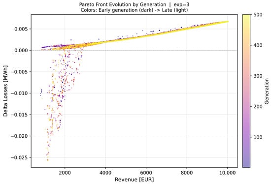
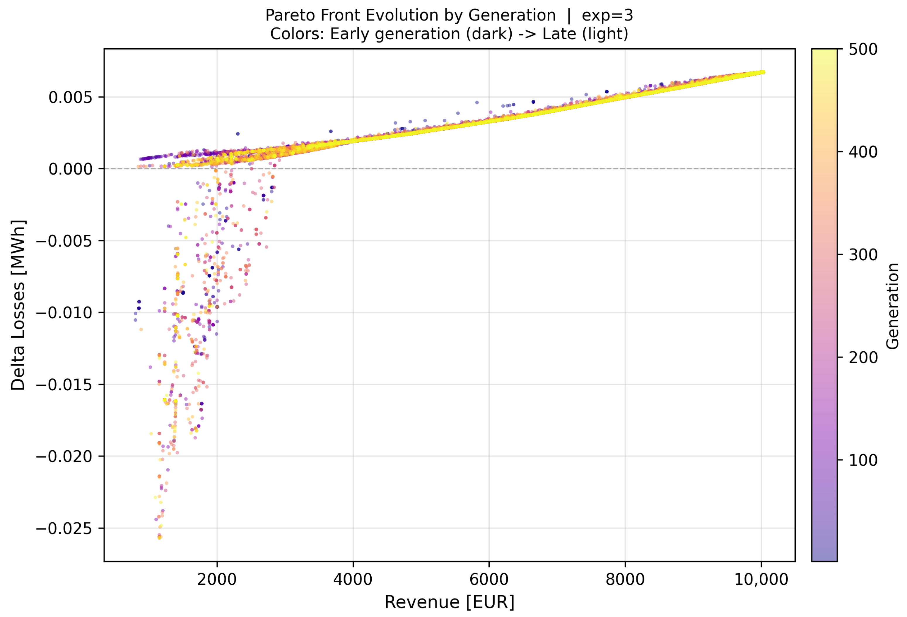
Figure 3 plots all stored non-dominated points across generations, colored from dark (early) to yellow (late), revealing the convergence dynamics of the Pareto front approximation.

Figure 3. Evolution of the Pareto front across 500 NSGA-II generations, Experiment 3. Each point represents one non-dominated solution recorded during the run; color encodes the generation number (dark purple: gen 1–50; yellow: gen 400–500). Revenue [€] is on the x-axis and the daily loss increment [MWh] relative to the base case on the y-axis (positive ΔLosses indicates that the BESS increases network losses). The wide dispersion of early generations compresses into a tight diagonal band by generation 200, signaling that the population has identified Bus 91 as the dominant location and is refining the trade-off along a well-defined Pareto curve.

Three phases are discernible. Early phase (gen 1–50, dark purple): the front is dispersed over a wide range of ΔLosses, from $-0.027$ to $+0.003$ MWh. Negative values indicate solutions at peripheral buses (8, 19, 48) where the BESS absorbs power during charging in a way that locally compensates flow on long lossy corridors; these solutions yield low revenue (<3000 €) and are progressively dominated as Bus 91 candidates emerge with both higher revenue and comparable loss figures. Transition phase (gen 50–200, orange/pink): the negative-loss tail shortens rapidly as NSGA-II selects against solutions that trade revenue for loss reduction when the $F_1$ penalty exceeds the $F_2$ gain under non-dominated sorting. The front rotates and compresses toward the positive-ΔLosses diagonal. Convergence phase (gen 200–500, yellow): the front solidifies into a dense monotone band spanning revenue from €1500 to €10,033 and ΔLosses from 0 to $6.7\times {10}^{-3}$ MWh. Band narrowing indicates that the population has exhausted exploration diversity and is refining crowding distance along an already well-approximated Pareto curve.

5.3. Final Pareto Front and Trade-Off Structure

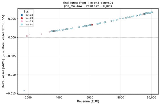
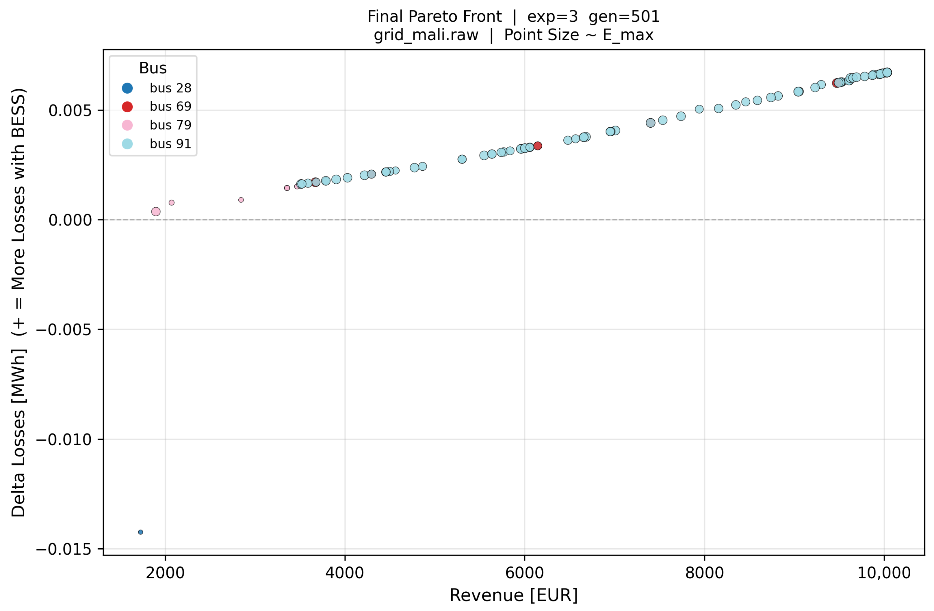
Figure 4 presents the final generation front (gen 501) with bus color and point size proportional to $E_{\max }$, providing a comprehensive view of the trade-off between revenue and loss impact across all surviving non-dominated solutions.

Figure 4. Final Pareto front, Experiment 3, gen 501, Mali grid. Point color encodes installation bus (cyan: Bus 91; red: Bus 69; pink: Bus 79; blue: Bus 28) and point size is proportional to $E_{\max }$ [MWh]. Revenue [€] is on the x-axis; daily loss increment [MWh] relative to the base case is on the y-axis. The revenue ceiling at €10,033 is a network limit—the required power saturates at least one branch thermal constraint at Bus 91—not a search-space boundary. Bus 28 (lower left) is the only location that actively reduces network losses below the base case.

The structure of Figure 4 confirms four distinct clusters. Bus 91 (cyan, dominant) spans revenue from €3500 to €10,033, with ΔLosses growing monotonically from $1.7\times {10}^{-3}$ to $6.7\times {10}^{-3}$ MWh. Point size increases with revenue, confirming that the algorithm allocates larger $E_{\max }$ to higher-revenue solutions. The revenue ceiling at €10,033 is not a search boundary but a network-imposed limit: beyond this level, the required charge/discharge power saturates at least one branch thermal limit in (8), rendering the DC-OPF sub-optimal or infeasible—a direct consequence of embedding network security as a hard constraint. Bus 69 (red) is concentrated around €6200 with ΔLosses $\approx 3\times {10}^{-3}$ MWh, and limited headroom due to existing base-case loading near the slack area. Bus 79 (pink) contains low-revenue solutions (€1800–3500) with near-zero ΔLosses, representing small BESS units at a peripheral bus with negligible network impact. Bus 28 (blue, isolated) is the sole solution with revenue €1727 and $\Delta \mathrm{Losses}=-1.42\times {10}^{-2}$ MWh, and is the only BESS location that actively reduces network losses relative to the base case by absorbing power that would otherwise flow over a long lossy corridor during the BESS charging period.

5.4. Optimal Dispatch Profiles

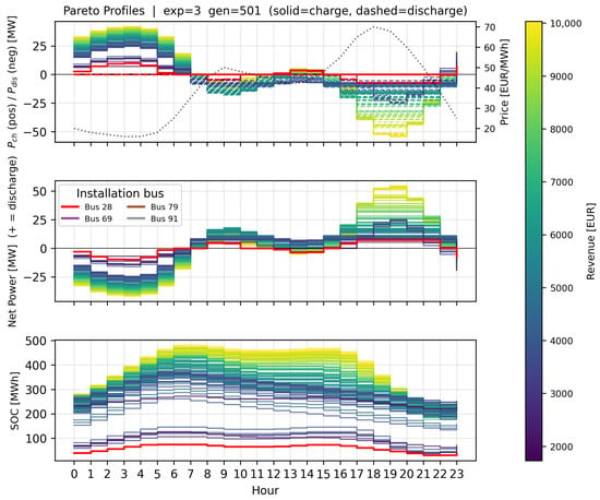
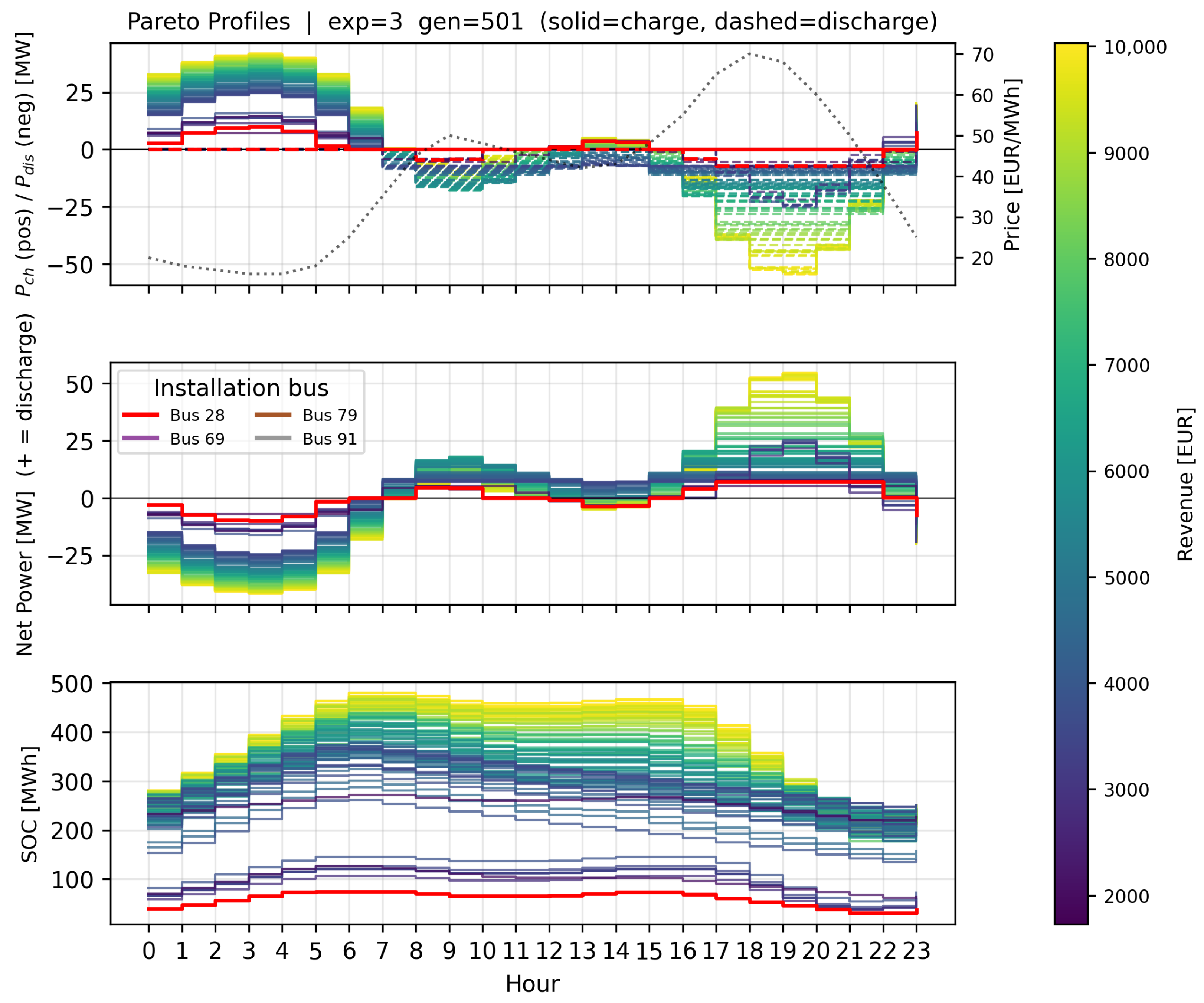
Figure 5 presents the complete operational profile of all non-dominated solutions from gen 501: charge/discharge power (top), net bus injection (middle), and SOC trajectory (bottom).

Figure 5. Hourly dispatch profiles for all Pareto-optimal solutions, Experiment 3, gen 501. Curve color encodes daily revenue [€] via the viridis colorbar; the compact legend identifies installation bus. (Top) charging power $P_{ch}$ [MW] (solid) and discharging power $P_{dis}$ [MW] (dashed); dotted curve shows price ${\pi }^{\left(t\right)}$ [EUR/MWh] on the right axis. (Middle) net bus injection [MW] (positive = discharge). (Bottom) SOC trajectory [MWh]; all solutions start and end at $0.5·E_{\max }$, satisfying the cyclic constraint (15).

Charge cycle (hours 3–9): all solutions charge during the low-price valley (€16–20/MWh). Charging power ramps from ∼10 MW at hour 3 to 35–40 MW by hours 6–7, then tapers as the price curve begins its morning rise. The SOC rises from the initial level $0.5·E_{\max }$ to a peak of 430–490 MWh (for Bus 91, $E_{\max }\approx 500$ MWh) reached around hour 9. The smooth ramp reflects the IPOPT optimizer trading off marginal charging cost against SOC headroom under the binding box constraint ${\mathrm{soc}}^{\left(t\right)}\le E_{\max }$.

Discharge cycle (hours 17–21): discharge begins as prices exceed the cycle break-even (€∼45/MWh) and peaks at hours 17–18 during the duck-curve afternoon price spike (€65–70/MWh). Net discharge power reaches 40–45 MW at Bus 91. The SOC returns to $0.5·E_{\max }$ at hour 24, satisfying constraint (15). The near-identical dispatch profiles across all high-revenue Bus 91 solutions confirm that the DC-OPF is saturating the same binding branch constraints regardless of the exact $P_{ch,\max }$, $P_{dis,\max }$, or $E_{\max }$ values, consistent with the revenue ceiling at €10,033.

6. Conclusions

This paper has presented and validated a hierarchical multi-objective BESS planning framework applied to the 130-bus Mali transmission network. The key results and takeaways are as follows.

Computational tractability via EDCPF and PTDF. A full AC power flow at every NSGA-II evaluation would require $\mathcal{O}\left(n^3\right)$ work per Newton–Raphson iteration across $T·N_{pop}·N_{gen}\approx 15\times {10}^6$ evaluations for the 500-generation experiment. The vectorized EDCPF model and pre-computed PTDF matrix reduce this to a single KLU back-substitution per time step, making the optimization feasible in hours on a standard workstation without approximating network physics beyond the DC linearization standard in transmission planning.

Network security as a hard constraint. Embedding PTDF-based thermal limits inside the lower-level NLP ensures that every Pareto solution in Figure 3 and Figure 4 corresponds to a thermally feasible dispatch. The revenue ceiling at €10,033 directly reflects the binding branch limits at Bus 91, not a search-space boundary; penalty-based approaches would produce apparent solutions above this ceiling that are physically infeasible.

Economic vs. technical impact on the Mali network. The Pareto front reveals a nearly linear positive correlation between revenue and loss increment for Bus 91. Achieving maximum revenue (€10,033/day) costs a loss increment of $6.7\times {10}^{-3}$ MWh/day, which is small relative to the economic gain. The only solution actively reducing losses is Bus 28 ($\Delta \mathrm{Losses}=-1.42\times {10}^{-2}$ MWh), at the cost of revenue dropping to €1727/day. For a Mali system operator where network reliability is the primary concern, Bus 28 may be technically preferable despite its lower economic return.

Star-bus TR3W expansion. The five three-winding transformers are handled transparently through star-bus expansion in the PSS/E RAW parser, preserving admittance fidelity in $\mathbf{B}$ without requiring special-case logic in the PTDF or OPF formulations.

Cyclic SOC constraint. Fixing ${\mathrm{soc}}^{\left(0\right)}={\mathrm{soc}}^{\left(T\right)}=0.5·E_{\max }$ prevents revenue inflation from horizon-end discharge and makes single-day results a valid proxy for steady-state long-term operation, as confirmed by the closed SOC trajectories in Figure 5.

Comparison with alternative approaches. Single-objective LP formulations [7,13] identify a revenue-maximizing or loss-minimizing schedule efficiently but collapse the planning problem to a single operating point, losing the trade-off information essential for investment decisions in resource-constrained grids. Multi-objective evolutionary methods without network constraints [14,15] preserve the Pareto structure but risk physically infeasible solutions when penalty weights are poorly tuned. The proposed framework avoids both limitations: it retains the full Pareto front while guaranteeing thermal feasibility through hard PTDF constraints. The main trade-off relative to full AC OPF formulations is the DC linearization error, acceptable for long-term transmission planning but with the voltage and reactive power limitations discussed above.

Limitations. Five limitations of the current framework should be acknowledged. First, the DC linearization assumes negligible branch resistances, uniform voltage magnitudes, and small angle differences. While standard in transmission planning, this means that reactive power flows and voltage magnitude violations are not captured; the EDCPF layer partially corrects loss estimates but does not enforce voltage bounds as hard constraints.

Second, the BESS is modeled with fixed efficiencies ${\eta }_{ch}={\eta }_{dis}=0.95$ and no degradation model. As a result, the projected daily revenue figures represent upper bounds on long-term economic performance, since capacity fade reduces effective $E_{\max }$ over time [36,37].

Third, the optimization uses a single deterministic 24 h price and load profile. No stochasticity in prices, generation, or demand is modeled. The cyclic SOC constraint makes individual-day results self-consistent, but a multi-day stochastic extension is needed to quantify planning robustness under uncertainty.

Fourth, the framework optimizes a single BESS unit. The coordinated placement of multiple units could achieve additional loss reduction through complementary injection profiles at different network nodes.

Fifth, network security is verified only for the base-case topology. No N-1 contingency analysis is performed; a Pareto-optimal solution under normal operation may violate branch limits following the outage of a line adjacent to Bus 91.

Future work will also benchmark the Pareto front against a reference AC optimal power flow to quantify the accuracy loss of the DC approximation on this specific network topology.

References

- Peças Lopes, J.A.; Hatziargyriou, N.; Mutale, J.; Djapic, P.; Jenkins, N. Integrating distributed generation into electric power systems: A review of drivers, challenges and opportunities. Electr. Power Syst. Res. 2007, 77, 1189–1203. [Google Scholar] [CrossRef] [Scilit]
- Scrocca, A.; Pisani, R.; Andreotti, D.; Rancilio, G.; Delfanti, M.; Bovera, F. Optimal spot market participation of PV + BESS: Impact of BESS sizing in utility-scale and distributed configurations. Energies 2025, 18, 3791. [Google Scholar] [CrossRef] [Scilit]
- African Review. Power Transmission in Africa: Challenges and the Way Ahead; African Review of Business and Technology: London, UK, 2024. [Google Scholar]
- The World Bank. Mali Electricity Sector Emergency Project (MESEP): Project Information Document/Integrated Safeguards Data Sheet. In World Bank Document; Report No. PIDISDSC24182; The World Bank: Washington, DC, USA, 2018. [Google Scholar]
- African Development Bank Group. Desert-to-Power Roadmap for Mali; Technical Report; African Development Bank Group: Abidjan, Côte d’Ivoire, 2020; Available online: https://www.afdb.org/ (accessed on 15 January 2025).
- Levron, Y.; Guerrero, J.M.; Beck, Y. Optimal power flow in microgrids with energy storage. IEEE Trans. Power Syst. 2013, 28, 3226–3234. [Google Scholar] [CrossRef] [Scilit]
- Gill, S.; Kockar, I.; Ault, G.W. Dynamic optimal power flow for active distribution networks. IEEE Trans. Power Syst. 2014, 29, 121–131. [Google Scholar] [CrossRef] [Scilit]
- Avendaño Peña, Á.A. Dimensionamiento y Localización Óptima de Sistemas de Almacenamiento de Energía a Gran Escala para Reducir el Costo por Restricciones de Red en el Sistema Eléctrico Colombiano. Master’s Thesis, Universidad Nacional de Colombia, Manizales, Colombia, 2022. [Google Scholar]
- Overbye, T.J.; Cheng, X.; Sun, Y. A Comparison of the AC and DC Power Flow Models for LMP Calculations; University of Illinois at Urbana-Champaign: Urbana, IL, USA, 2003. [Google Scholar]
- Li, M.; Du, Y.; Mohammadi, J.; Crozier, C.; Baker, K.; Kar, S. Numerical comparisons of linear power flow approximations: Optimality, feasibility, and computation time. arXiv 2021, arXiv:2207.05216v1. [Google Scholar]
- Stott, B.; Jardim, J.; Alsac, O. DC power flow revisited. IEEE Trans. Power Syst. 2009, 24, 1290–1300. [Google Scholar] [CrossRef] [Scilit]
- Fraile López, J. Modelo de Despacho Económico Incluyendo Restricciones de Red; Universidad Pontificia Comillas—ICAI: Madrid, Spain, 2018. [Google Scholar]
- López-Ramos, F.; Nasini, S.; Sayed, M.H. An integrated planning model in centralized power systems. Eur. J. Oper. Res. 2020, 287, 361–377. [Google Scholar] [CrossRef] [Scilit]
- Qin, H.; Li, K.; Chen, Z. Non-Pareto genetic algorithm for optimal planning of multi-type energy resources in active distribution networks. Front. Energy Res. 2022, 10, 966549. [Google Scholar] [CrossRef] [Scilit]
- Su, R.; He, G.; Su, S.; Duan, Y.; Cheng, J.; Chen, H.; Wang, K.; Zhang, C. Optimal placement and capacity sizing of energy storage systems via NSGA-II in active distribution network. Front. Energy Res. 2023, 10, 1073194. [Google Scholar] [CrossRef] [Scilit]
- Deb, K.; Pratap, A.; Agarwal, S.; Meyarivan, T. A fast and elitist multiobjective genetic algorithm: NSGA-II. IEEE Trans. Evol. Comput. 2002, 6, 182–197. [Google Scholar] [CrossRef] [Scilit]
- Andersson, J.A.E.; Gillis, J.; Horn, G.; Rawlings, J.B.; Diehl, M. CasADi: A software framework for nonlinear optimization and optimal control. Math. Program. Comput. 2019, 11, 1–36. [Google Scholar]
- Liu, D.; Liu, L.; Cheng, H.; Zhang, S.; Xin, J. An extended DC power flow model considering voltage magnitude. J. Mod. Power Syst. Clean Energy 2021, 9, 679–683. [Google Scholar] [CrossRef] [Scilit]
- Li, X.; Hedman, K. Data-driven linearized AC power flow model with regression analysis. arXiv 2018, arXiv:1811.09727v1. [Google Scholar]
- Bañol Arias, N.; López, J.C.; Hashemi, S.; Franco, J.F.; Rider, M.J. Multi-objective sizing of battery energy storage systems for stackable grid applications. IEEE Trans. Smart Grid 2021, 12, 2708–2721. [Google Scholar] [CrossRef] [Scilit]
- Tractebel Engineering S.A. Update of the ECOWAS Revised Master Plan for the Development of Power Generation and Transmission of Electrical Energy; Final Report; ECOWAS/WAPP: Paris, Franch, 2018. [Google Scholar]
- The World Bank. OMVS—Transmission Expansion Project: Project Appraisal Document. In World Bank Document; Report No. PAD1393; The World Bank: Washington, DC, USA, 2017. [Google Scholar]
- Pan, D.; Zhang, L.; Wang, B.; Jia, J.; Song, Z.; Zhang, X. Multi-objective planning of integrated energy system based on CVaR under carbon trading mechanism. Front. Energy Res. 2024, 12, 1310301. [Google Scholar] [CrossRef] [Scilit]
- Pérez Hernández, G. DMS Para el Control de Frecuencia en Micro-Redes Mediante la Gestión de BMS. Ph.D. Thesis, Universidad Autónoma de Nuevo León, Nuevo Leon, Mexico, 2020. [Google Scholar]
- Davis, T.A.; Natarajan, E.P. Algorithm 907: KLU, a direct sparse solver for circuit simulation problems. ACM Trans. Math. Softw. 2010, 37, 36. [Google Scholar] [CrossRef] [Scilit]
- Bohórquez-Bautista, K.J.; Moreno-Arias, D.A.; Montoya-Giraldo, O.D.; Gil-González, W.J. Comparative methods for solving optimal power flow in distribution networks considering distributed generators: Metaheuristics vs. convex optimization. Tecnura 2022, 26, 87–129. [Google Scholar] [CrossRef] [Scilit]
- Olivares, D.; Cañizares, C.; Kazerani, M. A centralized energy management system for isolated microgrids. IEEE Trans. Smart Grid 2014, 5, 1864–1875. [Google Scholar] [CrossRef] [Scilit]
- Attarha, A.; Scott, P.; Thiébaux, S. Network-aware co-optimisation of residential DER in energy and FCAS markets. Electr. Power Syst. Res. 2020, 189, 106730. [Google Scholar] [CrossRef] [Scilit]
- Martín-Crespo, A.; Hernández-Serrano, A.; Izquierdo-Monge, Ó.; Peña-Carro, P.; Hernández-Jiménez, Á.; Frechoso-Escudero, F.; Baeyens, E. AC/DC optimal power flow and techno-economic assessment for hybrid microgrids: TIGON CEDER demonstrator. Front. Energy Res. 2024, 12, 1399114. [Google Scholar] [CrossRef] [Scilit]
- Hassan, A.; Dvorkin, R.; Deka, D.; Chertkov, M. Optimal placement and sizing of battery energy storage systems in power grids. Appl. Energy 2022, 305, 117947. [Google Scholar]
- ANDRITZ Group. Manantali—Overhaul and Update of Five Units in the Republic of Mali; ANDRITZ Hydropower: Graz, Austria, 2014. [Google Scholar]
- Nygaard, I.; Kamissoko, F.; Nørgård, P.B.; Badger, J.; Dewilde, L. Feasibility of wind power integration in weak grids in non-coastal areas of sub-Saharan Africa: The case of Mali. AIMS Energy 2017, 5, 557–584. [Google Scholar] [CrossRef] [Scilit]
- African Development Bank Group; NEPAD-IPPF. Project Information Memorandum: 330 kV WAPP Ghana–Burkina–Mali Interconnection Project; African Development Bank Group: Tunis, Tunisia, 2019. [Google Scholar]
- Dembélé, Y.; Bonkaney, A.L.; Sanogo, S.; Kumar, N.; Tischbein, B.; Madougou, S. Performances analysis of on-grid-tied large-scale solar PV plant in Mali: A case study in Kita. Smart Grid Renew. Energy 2025, 16, 35–56. [Google Scholar] [CrossRef]
- Sánchez Molina, P. Científicos evalúan la rentabilidad y el impacto de los sistemas BESS en el mercado eléctrico español. pv Magazine España, 20 January 2026.
- Hesse, H.C.; Schimpe, M.; Kucevic, D.; Jossen, A. Lithium-ion battery storage for the grid—A review of stationary battery storage system design tailored for applications in modern power grids. Energies 2017, 10, 2107. [Google Scholar] [CrossRef] [Scilit]
- Wang, J.; Liu, P.; Hicks-Garner, J.; Sherman, E.; Soukiazian, S.; Verbrugge, M.; Tataria, H.; Musser, J.; Finamore, P. Cycle-life model for graphite-LiFePO4 cells. J. Power Sources 2011, 196, 3942–3948. [Google Scholar] [CrossRef] [Scilit]
Disclaimer/Publisher’s Note: The statements, opinions and data contained in all publications are solely those of the individual author(s) and contributor(s) and not of MDPI and/or the editor(s). MDPI and/or the editor(s) disclaim responsibility for any injury to people or property resulting from any ideas, methods, instructions or products referred to in the content. |
© 2026 by the authors. Licensee MDPI, Basel, Switzerland. This article is an open access article distributed under the terms and conditions of the Creative Commons Attribution (CC BY) license.