


Abstract
Associated gas in the Permian Basin is a methane-rich but spatially fragmented and intermittently available feedstock. Methane pyrolysis can convert hydrocarbons to hydrogen and solid carbon without forming process CO2 in the reactor, but its practical value depends on the captured-gas capacity factor, feed composition, high-temperature heat supply, product purification, continuous carbon withdrawal, carbon offtake, and transparent greenhouse-gas accounting. This study presents an implemented screening model for a modular 1 million standard cubic feet per day (MMSCFD) Permian associated-gas unit. A representative Permian composition is evaluated with hydrocarbon cracking stoichiometry, catalytic and thermal conversion envelopes, a net hydrogen recovery assumption, an energy-duty allocation, a levelized-cost model, and a well-to-gate carbon-intensity model. The catalytic base case produces 3.78 t/d of saleable H2 after 90% pressure-swing adsorption (PSA) recovery and 14.27 t/d of solid carbon; the thermal near-complete conversion bound produces 4.31 t/d of saleable H2 and 16.15 t/d of solid carbon. At a 0.85 capacity factor, $10 million installed capital expenditure (CAPEX), 8% real discount rate, 20-year life, 10 kWh per kg H2 energy intensity, and $0.06 per kWh electricity, the deterministic plant-gate levelized cost of hydrogen (LCOH) is $1.81 per kg H2 at zero carbon value and $1.05 per kg H2 at a net realized carbon value of $0.20 per kg C. Monte Carlo analysis over capacity factor, CAPEX, energy intensity, electricity price, carbon value, feed/capture cost, and yield uncertainty gives levelized cost of hydrogen values at the 10th, 50th, and 90th percentiles (P10/P50/P90) of $1.32/$1.91/$2.57 per kg H2. The corresponding screening carbon-intensity distribution is 2.34/4.11/5.89 kg carbon dioxide equivalent (CO2e) per kg H2, dominated by electricity carbon intensity and upstream methane loss. Geothermal or waste-heat preheat is treated quantitatively as a partial offset to low- and mid-temperature duties, not as a replacement for high-grade 900–1200 °C trim heat. The pathway is benchmarked against steam methane reforming, autothermal reforming with carbon capture and storage, electrolysis, small-scale liquefied natural gas, and gas-to-liquids conversion. Reported LCOH values are plant-gate production costs; separate hydrogen-logistics and negative-carbon-value stress tests identify conditions under which remote delivery or carbon disposal can erode the apparent economic advantage.
1. Introduction
Hydrogen is already a strategic feedstock for ammonia, refining, methanol, and several emerging industrial decarbonization routes. Hydrogen can be produced through multiple fossil, biomass, electrochemical, and thermochemical routes, each with different cost, carbon-intensity, and infrastructure requirements [1]. Yet most hydrogen production remains coupled to fossil conversion pathways, and low-emission hydrogen projects face cost, infrastructure, and policy uncertainty. The U.S. National Clean Hydrogen Strategy and Roadmap also emphasizes that hydrogen deployment depends not only on production technology but also on end-use demand, infrastructure, storage, and delivery systems [2]. The International Energy Agency continues to track a rapid but uneven low-emissions hydrogen pipeline, with project realization constrained by cost gaps, demand uncertainty, infrastructure, and electricity-market conditions [3]. This creates space for transitional pathways that can use existing hydrocarbon infrastructure while lowering direct process emissions and reducing wasteful gas disposal.
Oil-dominant basins such as the Permian co-produce large volumes of associated gas. Where gathering, compression, or processing capacity is constrained, this gas may be flared, curtailed, or sold into weak local markets. The global context remains material: the World Bank’s 2025 Global Gas Flaring Tracker reported 151 billion cubic meters of gas flared in 2024, the highest level since 2007 [4]. At individual oilfield sites, however, associated gas is not a uniform baseload resource. It is distributed, compositionally variable, and frequently intermittent. A single flare site may be too small for conventional gas monetization, while a pad cluster may have enough volume only after aggregation and buffering [5].
Methane pyrolysis, often described as turquoise hydrogen when the solid carbon is retained and not oxidized, decomposes methane according to CH4 → C(s) + 2H2. The reaction avoids direct reactor CO2 formation because carbon leaves as a solid rather than as CO2. This feature is attractive for associated-gas utilization, but it does not by itself guarantee low carbon intensity or economic viability. The practical outcome is controlled by the energy source used for the endothermic reaction, upstream methane emissions, electricity carbon intensity, feed intermittency, hydrogen purification, carbon solids handling, and the market value or disposal route for the carbon co-product [6,7,8,9].
The purpose of this paper is therefore narrower and more defensible than a broad deployment proposal. It provides an implemented screening-level model for Permian associated-gas methane pyrolysis and uses that model to quantify the sensitivity of hydrogen yield, LCOH, and carbon intensity to the variables most likely to determine field deployment. The work is not presented as a validated process design or 45V eligibility demonstration. Instead, it is a reproducible screening article with explicit assumptions, uncertainty ranges, and validation requirements.
1.1. Literature Positioning and Research Gap
The recent methane-pyrolysis literature has advanced rapidly across catalytic, plasma, thermal, microwave, and molten-media concepts [6,7]. Reviews emphasize the same recurring scale-up constraints: high-temperature heat supply, methane conversion at practical residence times, catalyst deactivation, carbon deposition and product quality, and the need for continuous solids removal. Molten metal and molten salt reactors are promising because they improve heat transfer and may reduce wall fouling, but the literature also shows that carbon removal is an unresolved scale-up issue rather than a peripheral detail [8].
Techno-economic studies of turquoise hydrogen often show attractive costs only when a low-cost heat source, high capacity factor, and valuable carbon product are assumed. This is a high-risk combination for flare or associated gas because the feedstock may be intermittent, carbon offtake may be limited by purity and logistics, and hydrogen purification and compression can be significant at modular scale. Prior studies have often focused on pipeline-quality methane or centralized plants; few have evaluated distributed associated gas with explicit capacity-factor and MRV uncertainty. Prior TEA studies also show strong sensitivity to energy supply, reactor assumptions, carbon value, and system configuration [10].
The flaring and associated-gas monetization literature typically focuses on gas gathering, power generation, small-scale LNG, CNG, mini-GTL, methanol, or gas-to-wire applications [4,11,12]. These are relevant alternatives because they compete for the same stranded feedstock. However, most alternatives monetize methane as energy or liquids rather than producing hydrogen. Conversely, the low-carbon hydrogen literature tends to benchmark SMR, ATR + CCS, and electrolysis, while treating flare gas as a special case mainly through renewable natural gas or alternative-fate frameworks [3,13,14,15,16,17,18,19]. This paper bridges those bodies of work by evaluating pyrolysis as one route among multiple associated-gas utilization options, not as an isolated reactor concept.
The final research gap addressed here is methodological. Many pathway studies present plausible process concepts without making the calculation boundary, feed composition, conversion assumptions, energy inputs, cost equations, uncertainty distributions, and limitations fully reproducible. For associated-gas conversion to hydrogen, this gap is especially important because feed intermittency, flare-measurement bias, methane leakage, carbon-product fate, and pathway-specific regulatory accounting can dominate the result. This study therefore implements a transparent screening workflow and avoids implying formal regulatory eligibility when the accounting tool does not contain the pathway. DOE’s 45VH2-GREET Rev. December 2025 evaluates well-to-gate emissions for pathways included in the model and states that methane pyrolysis is not retained in 45VH2-GREET, even though other GREET versions may include technologies not present in the 45V tool [15,20].
1.2. Novel Contribution of This Work
- An implemented mass-balance model for a representative 1 MMSCFD Permian associated-gas stream, including catalytic and thermal conversion envelopes, inert load, H2S pretreatment load, PSA recovery, tail gas, and carbon output.
- A transparent TEA model that reports deterministic and Monte Carlo LCOH values and identifies capacity factor, CAPEX, electricity price, energy intensity, and carbon value as the dominant drivers.
- A screening carbon-intensity model with a 1 kg H2 functional unit, a well-to-gate boundary, explicit electricity and methane-leakage sensitivities, and no unsupported claim of formal 45V eligibility.
- A quantified treatment of geothermal or waste-heat preheat as a partial low-/mid-grade heat credit, not as a direct substitute for high-grade pyrolysis heat.
- A tighter pathway comparison against SMR, ATR + CCS, electrolysis, small-scale LNG, and GTL, clarifying which alternatives produce hydrogen and which only monetize the same associated gas.
2. Literature Context and Pathway Comparison
2.1. Methane Pyrolysis and Solid-Carbon Handling
The appeal of methane pyrolysis is thermodynamic- and accounting-related: the stoichiometric reaction produces H2 and solid carbon rather than H2 and CO2. The standard enthalpy requirement is about 75 kJ per mol CH4, equivalent to approximately 37.5 kJ per mol H2 or 5.2 kWh per kg H2 before sensible heating, heat losses, separation, compression, and operating inefficiencies. Methane pyrolysis has been reviewed as a bridge technology because it avoids direct reactor CO2 formation while shifting the key uncertainties to heat supply, solid-carbon handling, and carbon-product disposition [21]. Actual modular systems therefore require energy intensities above the thermodynamic minimum. The screening base case in this study uses 10 kWh per kg net H2, a value intended to include trim heat, purification, compression, and auxiliary losses, while sensitivity analysis spans 7.5–13 kWh per kg H2.
Reactor choice strongly affects the credibility of yield assumptions. Thermal pyrolysis can achieve high conversion at high temperature, but sustained operation typically requires reactor temperatures in the 900–1200 °C range or higher. Catalytic routes can lower apparent temperature requirements but introduce deactivation, sulfur tolerance, regeneration, and carbon-product contamination challenges [6,7]. Molten-media routes can improve heat transfer and reduce wall coking, but carbon withdrawal from a hot, corrosive, dense medium becomes a primary design challenge [8]. For this reason, the paper treats thermal conversion as a yield upper bound and catalytic conversion as the economic base case.
Solid carbon is not treated as an automatic economic credit. Its net value depends on the morphology, purity, ash and metal contamination, particle-size distribution, moisture, stabilization, packaging, transportation, storage, customer qualification, and final disposition. If no qualified buyer or durable-use pathway exists, the net value may be negative because cooling, collection, packaging, transport, controlled storage, or disposal costs remain. Accordingly, the analysis distinguishes market-available cases, in which the net realized carbon value is zero or positive, from a disposal-liability stress case of −$0.10 kg−1 C. This negative value is an illustrative stress test rather than a universal disposal tariff. It represents the possibility that solid-carbon management creates a project cost rather than a revenue stream [6,7].
2.2. Flare-Gas Measurement, MRV Uncertainty, and Associated-Gas Utilization
Associated-gas utilization begins with measurement. Satellite products such as VIIRS Nightfire are essential for global and regional monitoring, but the recent literature indicates that small, intermittent, or enclosed flares can be missed or underestimated [11,22]. This matters because an economic model can be correct mathematically while still being wrong operationally if the assumed gas availability is biased. In this paper, MRV uncertainty is represented through capacity factor and feed/capture-cost uncertainty rather than by claiming a completed MRV dataset.
The most common flare-gas monetization alternatives are gathering-to-sales pipelines, gas-to-power, small-scale LNG or CNG, GTL, methanol, and NGL recovery [4,11,12]. Each competes on scale, capital intensity, logistics, and product market access. Small-scale LNG and CNG preserve methane as a fuel and require compression or liquefaction logistics. GTL converts methane into transportable liquids but requires reforming/syngas generation and Fischer–Tropsch synthesis, which adds complexity and CO2 management. Methane pyrolysis is different because it converts the gas to H2 and solid carbon, making carbon offtake and hydrogen delivery the central market risks. Hydrogen delivery is therefore treated as a separate deployment constraint rather than being embedded implicitly within production cost. Because transportation mode, distance, throughput, delivery pressure, storage requirements, and demand profile are site-specific, the plant-gate LCOH reported in this study should not be interpreted as the cost paid by a remote consumer. Delivered-cost implications are evaluated separately in Section Plant-Gate and Delivered Hydrogen Cost.
2.3. Hydrogen Benchmarks: SMR, ATR + CCS, and Electrolysis
SMR remains the conventional cost benchmark for natural-gas-derived hydrogen, while ATR + CCS is often the preferred new-build low-carbon reforming benchmark because capture integration can be more favorable for large, centralized facilities [14,17,18,19,23]. These pathways are more mature than methane pyrolysis and are explicitly represented in 45VH2-GREET under specified configurations [15,20]. Their disadvantages for isolated flare-gas applications are scale and CO2 logistics: a small, distributed associated-gas site may not have the scale or CO2 transport/storage access needed for conventional blue-hydrogen economics.
Electrolysis is the main non-fossil benchmark. Its carbon intensity can be very low with qualifying low-carbon electricity, but its economics depend strongly on electrolyzer CAPEX, power price, utilization, and grid interconnection. NREL and DOE assessments emphasize that current PEM electrolysis costs remain several dollars per kilogram under many U.S. conditions, while the IEA highlights large geographic differences in electrolyzer manufacturing and installation costs [3,13,14]. Recent machine-learning and AI-optimization work in PEM electrolysis shows how advanced modeling can improve cell and system operation, but it does not remove the need for low-cost electricity and high utilization [23,24,25]. The principal hydrogen-production and associated-gas monetization pathways considered in this study are summarized in Table 1.
Table 1.
Pathway positioning for Permian associated-gas monetization and hydrogen production.
2.4. Role of Data-Driven Optimization and AI-Based Screening
The recent hydrogen-production literature increasingly uses machine-learning surrogates, artificial neural networks, genetic algorithms, and hybrid optimization methods to accelerate design-space exploration. For this study, AI-based optimization is not treated as a substitute for physical mass and energy balances. Instead, it is positioned as a downstream layer that can rank candidate sites, select operating policies, and identify high-value measurements after the baseline stoichiometric, TEA, and CI models are specified. This distinction is important because a data-driven optimizer can find an apparent optimum even when the underlying reactor or cost model is poorly constrained; therefore, the physics-based screening model remains the core contribution.
For a Permian associated-gas deployment, AI or surrogate modeling is most defensible in three roles. First, a regression or probabilistic forecasting model can combine pad-level production history, gas–oil ratio, infrastructure distance, outage events, and remote-sensing detections to estimate the distribution of captured gas availability. Second, surrogate models can accelerate Monte Carlo propagation by approximating the relationship between feed composition, conversion, energy intensity, PSA recovery, and net hydrogen yield. Third, multi-objective optimization can identify trade-offs among LCOH, CI, capacity factor, carbon handling, and site logistics. The practical objective is not only to minimize cost but also to avoid designs that are cost-effective on paper while failing due to unstable feed, contaminant excursions, or a weak carbon offtake pathway.
The implementation used here therefore creates the minimum dataset that would be needed for later AI optimization: feed composition, conversion assumptions, output yields, economic drivers, CI drivers, and uncertainty ranges. Once field or pilot data become available, this framework can be upgraded from one-at-a-time and Monte Carlo screening to Bayesian updating, active learning, or surrogate-assisted optimization. This upgrade path directly addresses the need for recent hydrogen-production advances without overclaiming that an unvalidated AI model can resolve reactor scale-up, carbon withdrawal, or methane-emissions uncertainty.
3. Methods
The model is intentionally simple enough to reproduce in a spreadsheet or in Python 3.13.5 (Python Software Foundation, Beaverton, OR, USA) but detailed enough to answer the core reproducibility questions: What was modeled? What inputs were used? How were economics and carbon intensity calculated? Which uncertainties dominate? The analysis uses a 1 MMSCFD captured-gas case as a modular screening unit and scales linearly for smaller or larger capture volumes. The model does not assume that every flare site can deliver 1 MMSCFD; the 1 MMSCFD case is a convenient basis for evaluating modular clusters. Detailed unit conversions and the supporting mass-balance, techno-economic, and carbon-intensity equations are provided in Appendix A. All numerical calculations were performed using Python 3.13.5 with NumPy 2.3.5, and Matplotlib 3.10.8 was used for figure generation. No commercial chemicals, reagents, biological materials, physical samples, laboratory devices, or analytical instruments were used because this study is a numerical screening analysis.
3.1. System Boundary and Functional Unit
The process boundary includes captured associated gas at the plant battery limit, condensate knock-out, dehydration and H2S polishing, compression where needed, feed preheat and heat recovery, catalytic or thermal methane-pyrolysis conversion, carbon disengagement/withdrawal, product quench/cooling, pressure-swing adsorption (PSA), and H2 compression. Downstream hydrogen storage, transportation, distribution, dispensing, and end use are excluded from the plant-gate production boundary. Consequently, all LCOH values reported in the principal techno-economic analysis are plant-gate production costs. Section Plant-Gate and Delivered Hydrogen Cost introduces an additive logistics term for evaluating delivered hydrogen cost without conflating production and delivery. Carbon transportation, storage, and disposal are represented through the net realized carbon-value parameter. The TEA functional unit is one kilogram of saleable H2 after PSA recovery. The CI functional unit is one kilogram of 100% H2 on a well-to-gate basis, aligned conceptually with 45VH2-GREET’s functional-unit logic, but not represented as a formal 45VH2-GREET run because methane pyrolysis is not retained in the current 45VH2-GREET tool [15,20].
The system boundary deliberately separates three concepts that are often blended: (i) reactor stoichiometry and yield, (ii) economic value of carbon as a co-product, and (iii) policy accounting. Reactor stoichiometry can be calculated directly. Carbon value depends on product specifications and offtake. Policy accounting requires pathway-specific rules and official tools. This study calculates a transparent screening CI and does not claim 45 V qualification. The screening process boundary and the principal material and energy flows are illustrated in Figure 1.
Figure 1.
Process boundary used in the screening model. The high-temperature pyrolysis reactor still requires high-grade trim heat. Geothermal, waste heat, or recovered heat is credited only where temperature matching permits preheat or auxiliary duty offset.
3.2. Feedstock Composition and Availability
The base feed is a representative Permian associated/flare-gas composition previously used in the manuscript development and attributed to DOE/NETL associated-gas upcycling work [6]. It is not presented as a basin-wide average. It is a screening composition selected to test the implications of a methane-rich but wet and inert-containing feed. The gas contains 69.3 mol% CH4, 11.0 mol% C2H6, 4.7 mol% C3H8, 2.0 mol% C4H10, 1.1 mol% CO2, 10.1 mol% N2, 0.4 mol% H2S, and 1.4 mol% other inerts. The 1 MMSCFD standard feed corresponds to 1195 kmol/d. H2S is assumed to be removed upstream to less than 10 ppm using a guard-bed or sweetening step; CO2, N2, and other inerts are carried through the reactor and increase purification load.
Feed availability enters the model through the capacity factor rather than through a claimed MRV-grade forecast. For a given time interval, the captured feed is where Qcap,t is the captured gas rate during time interval t, Qavail,t is the available associated-gas rate, is the capture efficiency, and at is the equipment availability factor. The TEA combined effect is represented by the capacity factor, CF. The base case uses CF = 0.85, while sensitivity and Monte Carlo sampling span 0.45–0.95. This range is intentionally broad because field units tied to variable flare gas may run below steady industrial utilization unless gas is aggregated or buffered. The representative associated-gas composition and the treatment assigned to each feed component in the screening model are summarized in Table 2.
Table 2.
Baseline Permian associated-gas composition and feed basis.
3.3. Pyrolysis Conversion Model
Hydrocarbon cracking is represented by stoichiometric conversion of C1–C4 hydrocarbons to H2 and solid carbon:
The thermal near-complete conversion case is treated as a yield upper bound: = 0.99 and XC2 − C4 = 0.995. The catalytic base case is used for TEA: , , , and . These values are not claimed as kinetic predictions for a specific reactor; they are screening conversions used to quantify the economics and CI implications of a plausible modular catalytic pathway. The validation section below defines the pilot data required to replace these assumed conversions with reactor-specific kinetics.
Carbon dioxide is treated as non-reactive in the base mass balance because reactor-specific kinetic and catalyst data are unavailable. This is a simplifying modeling assumption rather than a claim that CO2 is chemically inert. At the modeled temperatures, CO2 may participate in the reverse water–gas shift reaction,
or methane dry reforming,
As a conservative upper-bound for sensitivity, complete reverse water–gas shift conversion of the 1.1 mol% inlet CO2 would consume approximately 13.1 kmol d−1 of H2, reducing net saleable hydrogen by approximately 24 kg d−1 after PSA recovery, or less than 1% of the catalytic base-case output. It would also produce approximately 13.1 kmol d−1 of CO requiring separation, recycling, oxidation, or controlled disposal. Complete dry reforming of the same CO2 quantity would additionally alter solid-carbon production and could produce approximately 26.3 kmol d−1 of CO. These calculations are bounding cases rather than kinetic predictions; reactor-specific modeling should include CO2 conversion, CO formation, water production, catalyst effects, and the associated separation and emissions costs. Dry reforming and reverse water–gas shift have been experimentally and kinetically demonstrated under elevated-temperature conditions, so acknowledging them is scientifically necessary.
Gross hydrogen production is calculated from the converted hydrocarbon feed as:
where K = {CH4, C2H6, C3H8, C4H10}, is the inlet molar flow of hydrocarbon k, Xk is the conversion of species k, and is the stoichiometric hydrogen yield coefficient.
Solid-carbon production is calculated as:
where is the molar mass of carbon and is the stoichiometric carbon yield coefficient.
Net saleable hydrogen after PSA recovery is:
where RPSA = 0.90 and
Tail gas contains unrecovered hydrogen, unconverted hydrocarbons, and inert species. It may be recycled, purged, or used as trim fuel depending on site integration. In the base economic model, however, trim energy is conservatively priced as purchased electricity or equivalent external energy input rather than assuming full tail-gas energy credit.
3.4. Energy, Heat-Integration, and Geothermal/Preheat Model
The energy model distinguishes the thermodynamic reaction requirement from practical delivered energy. The reaction enthalpy minimum is approximately 5.2 kWh per kg H2. The base economic model uses 10 kWh per kg net H2, which includes high-temperature trim heat, sensible heating not recovered by heat integration, gas purification and compression, controls, and other parasitic loads. The sensitivity range of 7.5–13 kWh per kg H2 covers better heat recovery and higher-loss modular operation.
Geothermal or waste-heat integration is credited only against heat duties that can be temperature-matched. A geothermal stream at 120–220 °C can offset feed preheat, dehydration regeneration, or other auxiliary thermal loads, but it cannot directly replace a 900–1200 °C reactor heat source. The quantitative preheat credit is therefore applied as an energy-intensity reduction of 0.5, 1.0, or 2.0 kWh per kg net H2. This approach directly answers the thermodynamic concern: geothermal helps economics and CI only modestly unless a high-temperature heat source is available, because most pyrolysis heat remains high-grade trim heat. The thermodynamic minimum, practical energy-intensity range, geothermal or waste-heat preheat credits, and base electricity assumptions used in the screening model are summarized in Table 3.
Table 3.
Energy and preheat assumptions used in the screening model.
3.5. Techno-Economic Model
The techno-economic analysis is reported on the basis of one kilogram of saleable hydrogen after PSA recovery. Capital and fixed operating costs are annualized and divided by annual net hydrogen production, while energy cost, feed/capture cost, and carbon-product credit are treated on a per kg H2 basis.
The capital recovery factor is calculated as:
where r is the real discount rate and N is project life in years.
Annual net hydrogen production is calculated as:
where CF is capacity factor and is daily net saleable hydrogen production.
The net realized carbon credit per kg H2 is:
where is daily solid-carbon production and is the net realized carbon value after handling, packaging, quality discounts, and logistics.
The parameter PC may be negative when carbon cooling, handling, transportation, stabilization, storage, or disposal costs exceed any realized sale value.
The levelized cost of hydrogen is then calculated as:
where I0 is installed CAPEX, CFOM is annual fixed operating and maintenance cost, is specific energy intenisity, is electricity price, is feed/capture cost per kg H2, and is the net carbon credit per kg H2. This structure follows the general Hydrogen Analysis (H2A) approach of transparent process-cost reporting, including capital, operating, energy, and financial assumptions [26,27,28].
The base case assumes r = 8%, N = 20 years, and fixed O&M equal to 4% of installed CAPEX per year. Installed CAPEX is assumed to be I0 = $10 million for a modular 1 MMSCFD catalytic unit including pretreatment, reactor, gas–solid separation, carbon-handling interface, PSA, and compression. This value is an order-of-magnitude screening assumption rather than a vendor quotation and varies from $7 million to $16 million in the Monte Carlo analysis.
For the catalytic base case, after 90% PSA recovery. At CF = 0.85, this corresponds to:
The carbon-value parameter is therefore treated as a net realized value, not as a guaranteed carbon-black or battery-grade market price. This conservative framing is necessary because projects cannot rely on premium carbon markets without product qualification, carbon-quality verification, and confirmed offtake. The principal techno-economic assumptions used in the deterministic base case and uncertainty analysis are summarized in Table 4.
Table 4.
Techno-economic assumptions for the catalytic base case.
Plant-Gate and Delivered Hydrogen Cost
The principal LCOH calculation represents hydrogen at the production-plant gate. Delivered hydrogen cost is expressed as:
where ccomp, cstor, ctrans, and cdisp are the incremental costs of downstream compression, storage, transportation, and dispensing, respectively. These terms depend on transport distance, hydrogen pressure, throughput, delivery mode, storage duration, and end-user demand. Therefore, a universal logistics cost is not assigned. To demonstrate the possible effect without implying site-specific precision, additive logistics burdens of $0, $1, $3, and $5 kg−1 H2 are evaluated. At zero realized carbon value, these assumptions increase the catalytic base-case cost from $1.81 kg−1 H2 at the plant gate to $1.81, $2.81, $4.81, and $6.81 kg−1 H2 delivered, respectively. At a net carbon value of $0.20 kg−1 C, the corresponding delivered costs are $1.05, $2.05, $4.05, and $6.05 kg−1 H2. These values are illustrative sensitivities rather than route-specific estimates. A project-level evaluation should use a delivery model such as the Hydrogen Delivery Scenario Analysis Model and specify distance, throughput, mode, pressure, storage, and demand [26,29]. Consequently, methane-pyrolysis hydrogen produced at remote associated-gas sites should not be compared with electrolysis located at the point of consumption unless both pathways use consistent delivery and storage boundaries.
3.6. Carbon-Intensity Model
The CI model is a screening well-to-gate calculation, not a formal regulatory certification. It includes electricity-related emissions and methane loss associated with the methane feed. It does not credit avoided flaring, because applying an alternative-fate credit to associated-gas methane pyrolysis would require a regulatory pathway and site-specific evidence not supplied here. The functional unit is 1 kg of saleable H2. The screening CI is:
with:
where is the well-to-gate carbon intensity in kg CO2e per kg H2, is energy intensity in kWh per kg H2, EFel is electricity carbon intensity in kg CO2e kWh per kg, is the methane loss fraction expressed as a decimal, is the methane-feed-to-net-hydrogen mass ratio, and CIother includes other upstream, or foreground emissions not explicitly modeled. This is much cleaner because the long methane-feed ratio is hidden inside
where EH2 is the energy intensity in kWh per kg H2, EFelectricity is electricity carbon intensity in kg CO2e per kWh, fCH4, loss is the methane loss fraction of methane feed, and GWP100 is the 100-year methane global-warming-potential factor. CIother is set to zero in the base screen but can be expanded to include chemicals, sorbents, compression equipment, carbon packaging, and transport. For deterministic illustration, EFelectricity = 0.40 kg CO2e per kWh is used because 45VH2-GREET Rev. December 2025 lists Texas at 0.40 kg CO2e per kWh [15]. Monte Carlo sampling uses 0.02–0.60 kg CO2e per kWh to capture renewable, hybrid, and grid-heavy cases.
The model treats solid carbon conservatively. If carbon is permanently stored or used in durable products, longer-term carbon retention may support lower lifecycle claims. If the carbon is later oxidized, the emissions must be included. Because the final fate of carbon is project-specific, this manuscript reports CI without a durable-carbon credit. This is more conservative than assuming carbon sequestration by default.
To improve readability and avoid ambiguity between molar flow, mass flow, annual production, and economic variables, the principal symbols used in the screening model are summarized in Table 5. Dotted variables denote flow rates, and methane-loss fraction is expressed as a decimal in equations. Broader GREET and hydrogen-pathway LCA resources include methane-pyrolysis and hydrogen-production pathway treatment outside the current 45VH2-GREET pathway set, but the present manuscript uses these sources only for contextual comparison rather than formal certification [30,31].
Table 5.
Notation used in the screening model.
3.7. Uncertainty Propagation
Uncertainty was propagated using direct Monte Carlo sampling implemented in Python 3.13.5 with NumPy 2.3.5. Matplotlib 3.10.8 was used only for figure generation. A fixed pseudorandom seed of 122 was used to permit exact reproduction. Each simulation consisted of 20,000 independent draws of capacity factor, installed CAPEX, energy intensity, electricity price, net realized carbon value, feed/capture cost, electricity carbon intensity, methane-loss fraction, and yield factor. Inputs were sampled independently because defensible correlation coefficients were unavailable. This independence assumption is retained as a limitation.
Percentile notation is used to report the Monte Carlo output distributions. In this manuscript, P10, P50, and P90 denote the 10th, 50th, and 90th percentiles, respectively. P50 is therefore the median of the simulated output distribution. This notation is used as distribution-percentile notation and not as petroleum-reserves probability-of-exceedance notation.
The simulation is a direct Monte Carlo calculation rather than a Markov chain Monte Carlo analysis. Therefore, burn-in periods, warm-up cycles, chain mixing, and Markov-chain convergence diagnostics are not applicable. Numerical stability was assessed by repeating the calculation with 5000, 10,000, 20,000, and 50,000 draws and comparing the resulting P10, P50, and P90 values. The maximum percentage change between the 20,000- and 50,000-draw results was 0.38% for LCOH percentiles only and 0.95% across all reported P10/P50/P90 outputs—LCOH, CI, and net H2 production.
For variables described by a minimum a, most-likely value m, and maximum b, the triangular probability-density function is:
The density integrates to unity over [a,b][a,b][a,b]; no post-sampling normalization or rescaling of the physical values is performed. Triangular distributions are used where lower and upper engineering bounds and a defensible most-likely value are available but insufficient observations exist to estimate an empirical distribution. This choice gives less weight to the extreme bounds than a uniform distribution. It is not assumed to be uniquely correct. The probability distributions and parameter values used in the Monte Carlo analysis are summarized in Table 6.
Table 6.
Uncertainty distributions used in Monte Carlo analysis.
For triangular distributions, values are listed as minimum, mode, and maximum. The yield factor follows a normal distribution with a mean of 1.0 and a standard deviation (SD) of 0.06, truncated to .
Because CAPEX is among the least constrained inputs, a distribution-form sensitivity was also performed by replacing the triangular CAPEX distribution with a uniform distribution over $7–16 million while retaining all other assumptions. The resulting P10/P50/P90 values are reported in Supplementary Materials. This check determines whether the principal conclusions depend on assigning a most-likely CAPEX value.
The effective capacity factor combines feed availability and reactor-system availability:
where Afeed represents associated-gas availability and Areactor represents reactor uptime after accounting for catalyst deactivation or poisoning, carbon fouling, solids-removal interruptions, planned maintenance, and unplanned shutdowns. The existing 0.45–0.95 capacity-factor range is interpreted through three screening scenarios:
CFeff = AfeedAreactor,
- “Worst case: 0.70 × 0.65 = 0.46;”
- “Base case: 0.90 × 0.94 = 0.85;”
- “Best case: 0.98 × 0.97 = 0.95.”
These values are scenario decompositions rather than measured reactor-availability predictions. Pilot operation is required to replace them with empirical uptime distributions.
3.8. Implemented Calculation Workflow
The model was implemented as a deterministic calculation followed by uncertainty propagation. The workflow is intentionally simple enough to be reproduced in a spreadsheet or Python script because, at the screening stage, transparent inputs are more useful than a black-box process simulator. The calculation sequence is as follows.
Step 1 defines the daily feed basis from the captured gas rate and standard molar volume. Step 2 multiplies the total molar flow by component mole fractions to obtain inlet kmol per d of CH4, C2H6, C3H8, C4H10, CO2, N2, H2S, and other inerts. Step 3 removes the H2S load as a pretreatment requirement and retains CO2, N2, and other inerts as non-reactive separation load. Step 4 applies the conversion envelope for each hydrocarbon species. Step 5 computes gross H2 and solid carbon using stoichiometric coefficients. Step 6 applies PSA recovery to obtain saleable H2 and collects unrecovered H2, inerts, and unconverted hydrocarbons as tail gas. Step 7 computes annual production from daily net H2 and the capacity factor. Step 8 computes LCOH from annualized CAPEX, fixed O&M, energy cost, feed/capture cost, carbon handling, and carbon revenue. Step 9 computes CI from energy carbon intensity and methane-loss terms. Step 10 samples uncertainty distributions and reports P10/P50/P90 outputs.
This implementation also prevents common overstatement. Gross H2 is not reported as the saleable product; it is reduced by purification recovery. Carbon is not automatically assigned a high premium value; it is treated as a net realized value after quality, packaging, logistics, and offtake constraints. Geothermal and waste heat are not credited as reactor-grade heat unless the temperature is compatible with the duty being offset. Methane leakage and electricity carbon intensity are kept explicit because they can dominate CI even when the reactor itself produces no direct CO2.
The same workflow can be scaled from a single flare to a pad cluster by changing the captured gas rate and capacity factor. It can also be extended to real time-series data by evaluating each time interval independently and aggregating daily or monthly hydrogen production, carbon output, LCOH, and CI. In that form, the model becomes a practical siting screen rather than a single static point estimate.
4. Results
4.1. Base-Case Mass Balance
Table 7 reports the implemented mass balance for the 1 MMSCFD feed. The catalytic base case produces 4204 kg per d gross H2 and 3783 kg per d net H2 after PSA recovery. It also produces 14,270 kg per d solid carbon. This carbon rate is not a minor by-product: it is approximately 3.77 kg C per kg H2 and therefore determines packaging, storage, handling, and offtake logistics.
Table 7.
Implemented pyrolysis mass balance for 1 MMSCFD captured associated gas.
4.2. Energy and Geothermal/Preheat Contribution
For the catalytic base case, the 10 kWh per kg H2 base energy intensity corresponds to 37.8 MWh per d of delivered energy at the 1 MMSCFD scale. The thermodynamic reaction minimum accounts for roughly 21.9 MWh per d of this value if expressed on a gross H2 basis, leaving the balance for sensible heating, heat losses, purification, compression, and auxiliaries. This split underscores why the energy model cannot be reduced to reaction enthalpy alone.
Table 8 quantifies the maximum economic and CI contribution of geothermal or waste-heat preheat under the base electricity price and Texas grid emission factor. A 1.0 kWh per kg H2 preheat credit lowers LCOH by only $0.06 per kg H2 and CI by about 0.40 kg CO2e per kg H2. Even a 2.0 kWh per kg H2 credit does not eliminate the need for high-grade trim heat. The conclusion is therefore not that geothermal makes pyrolysis low-cost by itself; rather, geothermal can modestly improve modular economics and CI where it is co-located and reliable.
Table 8.
Quantified preheat/geothermal contribution under base economic and CI assumptions.
4.3. Deterministic TEA and Capacity-Factor/Carbon-Value Map
The deterministic catalytic base case gives LCOH = $1.81 per kg H2 when the carbon product has zero net realized value. If net realized carbon value is $0.20 per kg C, LCOH decreases to $1.05 per kg H2 because the process produces 3.77 kg C per kg H2. This carbon credit is powerful, but also risky: without verified product quality and offtake, it should be treated as a sensitivity rather than as guaranteed revenue. At a capacity factor of 0.85, the catalytic case produces approximately 4.43 kt yr−1 of solid carbon. A net carbon value of −$0.10 kg−1 C therefore represents approximately $0.44 million yr−1 of carbon handling and disposal cost. Because the process produces approximately 3.77 kg C per kilogram of net H2, this downside assumption adds approximately $0.377 kg−1 H2 and increases plant-gate LCOH from $1.81 to approximately $2.19 kg−1 H2. Thus, the economic advantage can narrow substantially or disappear when carbon lacks a qualified market or controlled low-cost disposition route.
The contour map shows LCOH as a function of capacity factor and net realized solid-carbon value, with all other techno-economic inputs held at their base-case values. The base-case marker corresponds to a capacity factor of 0.85, a realized carbon value of $0.05 per kg C, and an LCOH of approximately $1.62 per kg H2. The capacity factor strongly controls cost because fixed capital and operating charges are spread over annual hydrogen output, while realized carbon value reduces cost only when carbon offtake is technically and commercially credible.
Figure 2 shows that a low capacity factor quickly overwhelms favorable co-product assumptions. The response surface shows that low capacity factor quickly overwhelms favorable co-product assumptions. At a CF below 0.60, modular units can struggle to compete even with a nonzero carbon value, because capital recovery and fixed O&M are spread over too little H2 production. This result is important for flare-gas deployment: an attractive reactor does not make a good project if the gas supply is too intermittent or if capture requires frequent start–stop operation.
Figure 2.
Deterministic plant-gate LCOH response surface for the catalytic modular methane-pyrolysis case. Net realized carbon value includes both positive product revenue and negative handling or disposal liability. The x-axis is extended to −$0.10 kg−1 C to show the negative-carbon-value stress case. At a capacity factor of 0.85, the −$0.10 kg−1 C stress case increases plant-gate LCOH to approximately $2.19 kg−1 H2, while the base-case marker remains at +$0.05 kg−1 C and approximately $1.62 kg−1 H2. Positive carbon values reduce LCOH only where product quality and offtake are technically and commercially credible.
4.4. Sensitivity and Uncertainty Analysis
Figure 3 shows one-at-a-time sensitivity around a base case with $0.05 per kg C net carbon value. The capacity-factor range in Figure 3 therefore corresponds to explicit worst-, base-, and best-case combinations of feed availability and reactor uptime rather than to an abstract utilization factor. The capacity factor, carbon value, CAPEX, and electricity price have the broadest impacts. Energy intensity matters, but within the selected range it is not the only determinant. This supports a practical deployment recommendation: early field screening should prioritize gas aggregation and uptime, power cost, and carbon offtake before attempting detailed optimization of a single reactor parameter.
Figure 3.
One-at-a-time sensitivity of levelized hydrogen cost for the catalytic modular methane-pyrolysis case. Each horizontal bar shows the LCOH range obtained by varying one input across the Table 6 sensitivity bounds while holding all other inputs at the base case. The dashed vertical line marks the base-case LCOH of $1.62 kg−1 H2, assuming a realized carbon value of $0.05 kg−1 C. The carbon value is varied from −$0.10 to +$0.20 kg−1 C, capturing both positive carbon-product revenue and negative carbon-handling or disposal liability. CAPEX, electricity price, realized carbon value, and capacity factor produce the widest cost ranges, indicating the parameters that most strongly control screening-level project economics.
The Monte Carlo analysis combines these uncertainties. The P10/P50/P90 LCOH values are $1.32/$1.91/$2.57 per kg H2. The median is higher than the deterministic zero-carbon base because the stochastic case includes feed/capture cost and a carbon-value distribution skewed toward low realized value. This is intentionally more conservative than treating carbon as a guaranteed high-value product. Figure 4 shows the Monte Carlo distribution of plant-gate LCOH and identifies the 10th, 50th, and 90th percentiles of the simulated results. The percentile results for plant-gate LCOH, carbon intensity, and net hydrogen production are summarized in Table 9.
Figure 4.
Monte Carlo uncertainty distribution for the catalytic modular methane-pyrolysis case. The histogram shows the levelized cost of hydrogen (LCOH) from 20,000 stochastic simulations of capacity factor, installed CAPEX, energy intensity, electricity price, realized carbon value, feed/capture cost, and yield uncertainty. The shaded region indicates the P10–P90 interval, while vertical markers identify P10 = $1.32 per kg H2, P50 = $1.91 per kg H2, and P90 = $2.57 per kg H2. The distribution emphasizes that the catalytic modular case should be interpreted as a screening-level cost range rather than a single deterministic value.
Table 9.
Monte Carlo screening results for LCOH, CI, and net H2 production.
4.5. Carbon-Intensity Results
The deterministic CI under the base energy intensity, Texas grid factor, and 0.3% methane loss is 4.31 kg CO2e per kg H2. Most of this is electricity-related. With low-carbon electricity, CI can fall sharply; with grid-heavy electricity and higher methane loss, CI can exceed the values often associated with blue-hydrogen benchmarks. The Monte Carlo CI distribution gives P10/P50/P90 values of 2.34/4.11/5.89 kg CO2e per kg H2. Figure 5 shows the sensitivity of well-to-gate carbon intensity to electricity carbon intensity and upstream methane loss fraction.
Figure 5.
Screening sensitivity of well-to-gate carbon intensity to electricity carbon intensity and methane loss fraction for the methane-pyrolysis case. Contours show estimated carbon intensity in kg CO2e per kg H2. Lower carbon intensity is achieved only when the electricity supply is low-carbon and upstream methane losses are tightly controlled, highlighting the dependence of screening-level CI estimates on site-specific power sourcing, methane management, and boundary assumptions.
Note: In the equation, is expressed as a decimal fraction. In Figure 5, methane loss is shown as a percentage for readability.
This result is central to manuscript credibility. Pyrolysis has no direct reactor CO2, but it is not automatically near-zero-carbon. The pathway’s CI depends on whether the trim heat is supplied with low-carbon electricity or fuel, whether upstream/capture methane leakage is controlled, and whether solid carbon remains unoxidized. The paper therefore reports CI as a sensitivity and uncertainty distribution rather than as a single claim.
4.6. Benchmark Against SMR, ATR + CCS, Electrolysis, LNG, and GTL
Table 10 compares methane pyrolysis with the principal hydrogen-production and associated-gas monetization alternatives, while Figure 6 presents the corresponding contextual carbon-intensity ranges. Table 10 and Figure 6 place the modeled pyrolysis case in context. SMR without CCS remains the low-cost incumbent but has high direct CO2 emissions. ATR/SMR with CCS can reduce CI materially at scale but requires CO2 capture, transport, and storage infrastructure. Electrolysis can be very low-carbon when powered by low-carbon electricity, but current costs are often higher and utilization can be constrained by power availability and hourly accounting requirements [3,13,14,15,16]. Small-scale LNG and GTL are not hydrogen pathways; they are gas monetization alternatives. They may be more logical where the primary objective is to move energy to a methane or liquid-fuel market rather than to produce H2.
Table 10.
Tighter comparison of methane pyrolysis with hydrogen and non-hydrogen associated-gas alternatives.
Figure 6.
Contextual well-to-gate carbon-intensity ranges for selected hydrogen-production pathways. The methane-pyrolysis range is derived from the present study. Reforming ranges are synthesized from References [12,14,15,16], and electrolysis ranges are synthesized from References [10,11,12,14,15,16]. The grid-electrolysis range reflects electricity consumption of approximately 50–55 kWh kg−1 H2 combined with grid-emissions factors of approximately 0.30–0.55 kg CO2e kWh−1. Ranges depend on the system boundary, methane leakage, capture performance, electricity source, allocation method, and site-specific data and should not be interpreted as formal regulatory determinations.
The comparison values in Table 10 and Figure 6 were not generated by the present methane-pyrolysis model. They are contextual ranges synthesized from the DOE, Argonne National Laboratory, National Petroleum Council, NREL, and related pathway assessments. Differences in system boundary, methane leakage, capture rate, electricity source, hydrogen pressure, and co-product allocation prevent direct equivalence; the ranges are therefore used only for screening context.
4.7. Interpreting the Comparison with Alternative Associated-Gas Pathways
The comparison in Table 10 should be read as a deployment-screening comparison rather than as a universal ranking. SMR remains economically attractive where gas supply is steady, plant scale is large, and CO2 management is not required. However, modular SMR is less naturally suited to fragmented flare-gas capture, and without CCS its CI is high relative to low-carbon hydrogen targets. ATR + CCS is often the stronger blue-hydrogen design at large scale because process CO2 can be captured more directly, but it requires CO2 transport and storage infrastructure and is difficult to justify for small, intermittent associated-gas volumes.
Electrolysis provides the cleanest pathway when powered by dedicated low-carbon electricity, but it does not directly solve associated-gas flaring unless the gas is separately gathered, processed, or displaced through another use. Its advantage is strongest where renewable electricity is abundant and hydrogen demand exists near the production site. Its disadvantage for the present problem is that the flare gas remains an unmanaged hydrocarbon stream unless the project includes a separate flaring-reduction strategy. For that reason, electrolysis is best treated as a hydrogen benchmark and potential competitor for clean-H2 offtake, not as a direct substitute for using captured associated gas.
Small-scale LNG and GTL are more direct associated-gas monetization alternatives because they convert stranded gas into transportable products [11,32]. LNG generally preserves methane as a fuel and can be attractive when trucking or nearby demand exists, but liquefaction adds energy demand and methane-slip risk, and small units require stable enough throughput to justify logistics. GTL can create liquid fuels compatible with existing distribution systems, but the process is more complex and carbon-intensive unless CO2 management is added. These options may be superior to pyrolysis where hydrogen offtake is absent or carbon-product markets are weak.
Methane pyrolysis therefore occupies a specific niche. It is most promising where associated gas can be clustered to maintain the capacity factor, where low-carbon electricity or high-value waste heat is available for high-grade duty, where carbon handling can be engineered continuously, and where a credible carbon offtake or disposal path exists. It is weakest where captured gas is sparse, intermittent, sulfur-rich, or located far from hydrogen users and carbon buyers. This nuanced positioning is more defensible than presenting pyrolysis as a universal replacement for SMR, ATR + CCS, electrolysis, LNG, or GTL.
5. Discussion
5.1. What the Results Imply for Permian Deployment
The main deployment insight is that reactor chemistry is only one part of the project. At the 1 MMSCFD modular scale, the base case can be economically interesting if the plant operates at a high capacity factor and can realize at least modest carbon value. The same unit becomes weak if the gas supply is intermittent, if power prices are high, or if carbon is a disposal cost instead of a product. Therefore, candidate sites should be ranked first by gas availability, aggregation potential, uptime, electrical interconnection, and offtake logistics, and only then by detailed reactor optimization.
The 57 MCFD single-flare equivalent illustrates the challenge. Scaling the catalytic base case linearly, 57 MCFD would produce only about 216 kg per d of net H2. That may be useful for local use or demonstration, but it is unlikely to support a full commercial H2 logistics chain unless multiple sites are aggregated. This supports a cluster model in which several pads feed a modular conversion unit or a mobile unit is deployed where gas availability is stable over a defined period.
Hydrogen Delivery and Market-Location Constraint
The plant-gate production cost should not be interpreted as delivered hydrogen cost. Hydrogen from a small remote associated-gas site may require compression, buffer storage, loading, trucking, unloading, additional compression, and customer-side storage. At the approximately 216 kg d−1 output estimated for a 57 MCFD single-flare equivalent, these fixed and scale-sensitive logistics can dominate the consumer cost. The strongest deployment cases are therefore likely to involve collocated hydrogen demand, aggregation of several pads into a larger hub, conversion to a transportable carrier, or sufficient throughput to justify dedicated pipeline infrastructure.
This consideration also changes the comparison with electrolysis. Electrolysis located at the point of consumption may have a higher plant-gate production cost but little or no long-distance hydrogen-delivery burden. Remote methane pyrolysis should therefore be compared with point-of-use electrolysis on a consistent delivery cost basis. The additive logistics sensitivity in Section Plant-Gate and Delivered Hydrogen Cost demonstrates that an apparent plant-gate advantage can be eliminated when transportation and storage costs reach several dollars per kilogram.
5.2. Capacity Factor Versus Process-Performance Improvements
A key deployment question is whether the capacity factor matters more than improvements in conversion, heat integration, or reactor performance. The results show that the capacity factor is a dominant filter because it affects annual H2 production over which capital and fixed O&M are spread. A moderate conversion or energy-intensity improvement can reduce LCOH, but a drop from CF 0.85 to 0.60 can add more cost than many process improvements remove. This finding creates a clear engineering insight: associated-gas pyrolysis is an uptime and logistics problem as much as a reactor problem.
Heat integration still matters, especially for CI and operating cost. However, geothermal preheat must be described carefully. The quantitative results show that a 1–2 kWh per kg H2 preheat credit is beneficial but not transformational. Geothermal integration becomes technically weak if it is presented as a complete heat source for 900–1200 °C pyrolysis. The manuscript therefore treats geothermal as a site-specific preheat and auxiliary heat option.
5.3. Continuous Carbon Withdrawal and Carbon-Market Uncertainty
The catalytic base case produces more than 14 t/d of solid carbon at only 1 MMSCFD. This converts carbon handling from a laboratory nuisance into a core process design requirement. Continuous withdrawal, gas–solid disengagement, sealing, cooling, packaging, and quality control must all be demonstrated. If carbon cannot be removed continuously, the plant loses capacity factor and the TEA deteriorates. If the carbon product is off-specification, the economic credit may disappear or become a disposal cost. Policy and market assessments similarly emphasize that methane-pyrolysis economics can depend heavily on whether solid carbon is qualified as a usable co-product rather than treated as a disposal burden [33].
The model therefore uses net realized carbon value and samples the distribution with a low mode. This prevents overclaiming while still showing the upside. A practical deployment assessment should state that carbon offtake is a development requirement, not an assumed outcome. The minimum publication-grade carbon data should include carbon purity, ash/metals content, particle-size distribution, surface area, morphology, moisture, packaging requirements, and a preliminary offtake or disposal pathway.
The present results quantify this downside explicitly. At the modeled 1 MMSCFD scale, carbon production exceeds hydrogen production by approximately 3.77:1 on a mass basis. Consequently, even a modest handling or disposal charge has a material effect on LCOH. Carbon should therefore be treated as a co-product only after its morphology, purity, contaminants, stability, customer specifications, annual market capacity, transportation distance, and final fate have been demonstrated. Otherwise, it should be modeled as a controlled waste stream with a negative net value. Uncontrolled environmental release is not considered an acceptable disposition pathway.
5.4. MRV, Satellite Bias, and Flare Availability
The revised paper avoids claiming that an MRV-grade forecasting framework has already been implemented. Instead, it treats MRV uncertainty through capacity-factor and feed-cost sensitivity and explains how a future field study would close the gap. Satellite observations are valuable for screening and regional estimation, but small and intermittent flares can be under-detected [11,22]. For a project-level TEA, the required evidence is meter data or a reconciled dataset combining operator metering, temporary field meters, aerial campaigns, and satellite observations.
A defensible project screening workflow would use satellite data to identify candidate clusters, field metering to validate volumes, gas chromatography to validate composition, and time-series analysis to estimate the monthly capacity factor. Without that evidence, the correct language is ‘screening’ or ‘preliminary feasibility,’ not deployment-grade or field-validated.
6. Validation Requirements and Limitations
The present model is suitable for screening-level assessment in an applied energy or engineering research context. It is not sufficient for investment-grade design, final tax-credit accounting, or reactor scale-up claims. The following limitations are explicit:
The feed composition is a representative screening mixture, not a basin-wide measured dataset. Field deployment requires site-specific gas chromatography and time-series metering.
The conversion model is stoichiometric with assumed conversion envelopes. It does not solve reactor kinetics, residence time, equilibrium, intraparticle diffusion, heat-transfer limitations, or catalyst deactivation.
The energy model uses a practical energy-intensity range rather than a detailed heat-exchanger network or Aspen/HYSYS simulation. Heat-integration claims must be updated if a process simulator is added.
The geothermal contribution is treated as a preheat credit only. No wellbore thermal model or field calibration is claimed in the revised paper.
The TEA uses screening CAPEX and O&M assumptions. Vendor quotes, detailed equipment sizing, and installation estimates are required before investment decisions.
The CI model is a transparent well-to-gate screen. It is not a formal 45VH2-GREET calculation or 45V eligibility determination, because methane pyrolysis is not retained in the current 45VH2-GREET pathway set [15,20].
Carbon value is uncertain and product-specific. The model does not assume that all solid carbon qualifies for premium carbon-black, graphite, or battery-material markets.
- Reported LCOH values are plant-gate production costs. Hydrogen compression, storage, transportation, distribution, and dispensing require route-specific analysis and may dominate delivered cost at low throughput.
- The base mass balance treats inlet CO2 as non-reactive. Reverse water–gas shift, dry reforming, CO formation, water formation, and their separation and emissions consequences require reactor-specific kinetic validation.
- Monte Carlo inputs are sampled independently because empirical correlation data are unavailable. Correlations among CAPEX, energy intensity, capacity factor, reactor availability, and carbon quality could widen or narrow the reported uncertainty intervals.
- The main Monte Carlo case represents market-available carbon scenarios. The separate negative-carbon-value case quantifies a disposal liability when no viable market exists.
Table 11 translates these limitations into validation requirements by naming the remaining gaps and specifying the data needed to close them.
Table 11.
Validation and limitations checklist for advancing from screening to field demonstration.
Validation Ladder for Moving Beyond Screening
A useful way to apply the limitations is to treat validation as a staged decision ladder. At the screening stage, the project only needs enough information to decide whether a site is worth detailed study: approximate gas composition, expected captured volume, candidate power price, carbon handling distance, and preliminary hydrogen offtake. At the pre-feasibility stage, the required evidence becomes stricter: time-series metering, gas chromatography, utility interconnection options, preliminary reactor vendor assumptions, and carbon-product characterization. At the pilot stage, the evidence must include continuous operation, closed carbon mass balance, measured energy use, contaminant tolerance, PSA performance, and controlled carbon withdrawal. At the field-demonstration stage, MRV reconciliation, methane monitoring, operating availability, maintenance frequency, and actual carbon sales or disposal costs become decisive.
This staged interpretation matters because the present paper intentionally avoids claiming that every site can produce low-carbon hydrogen. Instead, it asks whether a transparent screening model can identify the small subset of sites that deserve the next level of validation. A site with low LCOH but high methane-loss uncertainty is not yet a low-carbon site; it is a site where methane measurement should be prioritized. A site with strong gas availability but no carbon offtake is not yet economically attractive; it is a site where disposal cost, carbon quality, or non-premium carbon utilization must be tested. A site with apparent geothermal or waste-heat availability is not validated until measured temperature, flow, uptime, and parasitics show that the heat can actually offset a compatible process duty.
The same logic applies to the carbon product. The mass-balance results show that carbon production is several times larger than net H2 production by mass. That fact creates economic opportunity, but it also creates operational risk. Any final design must show how carbon is removed from the reactor, separated from catalyst or molten media, cooled, packaged, stored, shipped, or disposed of without interrupting hydrogen production. The validation ladder therefore treats continuous carbon withdrawal as a central gate rather than a peripheral equipment detail.
Finally, the CI model should be treated as a transparent foreground screen rather than a formal regulatory pathway calculation. For a future regulatory or certification claim, the authors should update the model to match the pathway recognized by the relevant program, use program-specific upstream emission factors, document electricity sourcing, and justify any allocation or displacement credit for the solid carbon product. Until that is done, the strongest defensible language is “screening well-to-gate CI” rather than “certified 45V-eligible hydrogen.”
7. Conclusions
- A representative 1 MMSCFD Permian associated-gas pyrolysis unit can produce approximately 3.78 t per d of net H2 and 14.27 t per d of solid carbon in the catalytic base case; the thermal near-complete conversion case provides a higher yield bound of 4.31 t pre d net H2 and 16.15 t per d C.
- The deterministic catalytic plant-gate LCOH is $1.81 kg−1 H2 at zero carbon value and $1.05 kg−1 H2 at a net realized carbon value of $0.20 kg−1 C. A negative carbon value of −$0.10 kg−1 C raises plant-gate LCOH to approximately $2.19 kg−1 H2, demonstrating that carbon disposition can be either a major benefit or a material liability.
- Monte Carlo analysis gives P10/P50/P90 LCOH values of $1.32/$1.91/$2.57 per kg H2. Capacity factor, CAPEX, electricity price, and carbon value dominate economics.
- Carbon intensity is not automatically low. The P10/P50/P90 screening CI distribution is 2.34/4.11/5.89 kg CO2e per kg H2, controlled mainly by electricity carbon intensity and methane loss.
- Geothermal or waste-heat preheat provides a modest quantified benefit but cannot replace high-grade pyrolysis heat. The revised framing is thermodynamically defensible because it credits only low-/mid-grade heat offsets.
- Compared with SMR, ATR + CCS, electrolysis, LNG, and GTL, methane pyrolysis is best framed as a modular hydrogen-and-carbon option for clustered associated gas where uptime, low-carbon energy, and carbon offtake are credible.
- The work is best interpreted as a full applied screening study rather than a field-validated design package. Stronger field-deployment claims require field MRV, reactor kinetics, continuous carbon-withdrawal data, heat-integration validation, carbon-quality evidence, and site-specific TEA/CI inputs.
- Reported LCOH values exclude downstream delivery. Additive logistics burdens of $1–5 kg−1 H2 can materially change or eliminate the apparent advantage over hydrogen produced near the point of consumption. The strongest deployment cases therefore require collocated demand, clustered production, or validated low-cost transportation infrastructure. Additional validation must include hydrogen logistics, reactor availability, CO2 side reactions, CO management, and evidence supporting either carbon offtake or controlled disposal cost.
Supplementary Materials
The following supporting information can be downloaded at: https://www.mdpi.com/article/10.3390/hydrogen7030095/s1.
Author Contributions
Conceptualization: A.T. and S.P.; methodology: A.T.; formal analysis: A.T.; writing—original draft: A.T.; writing—review and editing: A.T. and S.P.; supervision: M.W. and T.G. All authors have read and agreed to the published version of the manuscript.
Funding
This research received no external funding.
Data Availability Statement
All numerical results in the manuscript are reproducible from the equations, inputs, and distributions reported in Table 2, Table 3, Table 4 and Table 5. No proprietary field data are used. The calculation workbook and Monte Carlo code used to generate the reported mass-balance, LCOH, carbon-intensity, sensitivity, and uncertainty results are provided as Supplementary Materials. The code includes software-version information, the pseudorandom seed, distribution parameters, and the number of independent draws required to reproduce the reported percentiles.
Conflicts of Interest
The authors declare no known competing financial interests or personal relationships that could have appeared to influence the work reported in this paper.
Nomenclature
| Current | Use at first occurrence |
| MMSCFD | Million standard cubic feet per day (MMSCFD) |
| PSA | Pressure-swing adsorption (PSA) |
| CAPEX | Capital expenditure (CAPEX) |
| LCOH | Levelized cost of hydrogen (LCOH) |
| CI | Carbon intensity (CI) |
| TEA | Techno-economic analysis (TEA) |
| MRV | Measurement, reporting, and verification (MRV) |
| SMR | Steam methane reforming (SMR) |
| ATR | Autothermal reforming (ATR) |
| CCS | Carbon capture and storage (CCS) |
| 45V | Section 45V of the U.S. Internal Revenue Code (45V) |
| GTL | Gas-to-liquids (GTL) |
| LNG | Liquefied natural gas (LNG) |
| CNG | Compressed natural gas (CNG) |
| NGL | Natural gas liquids (NGL) |
| PEM | Proton-exchange membrane (PEM) |
| VIIRS | Visible Infrared Imaging Radiometer Suite (VIIRS) |
| GHSV | Gas hourly space velocity (GHSV) |
| CO2e | Carbon dioxide equivalent |
Glossary
P10, 10th percentile of the Monte Carlo output distribution; P50, 50th percentile or median of the Monte Carlo output distribution; P90, 90th percentile of the Monte Carlo output distribution; SD, standard deviation. AI, artificial intelligence; ATR, autothermal reforming; CAPEX, capital expenditure; CCS, carbon capture and storage; CF, capacity factor; CI, carbon intensity; CNG, compressed natural gas; DOE, U.S. Department of Energy; FOM, fixed operation and maintenance; GHG, greenhouse gas; GREET, Greenhouse gases, Regulated Emissions, and Energy use in Technologies; GTL, gas-to-liquids; HDSAM, Hydrogen Delivery Scenario Analysis Model; IEA, International Energy Agency; LCOH, levelized cost of hydrogen; LNG, liquefied natural gas; MMSCFD, million standard cubic feet per day; MRV, measurement, reporting, and verification; NGL, natural gas liquids; NREL, National Renewable Energy Laboratory; O&M, operation and maintenance; PEM, proton-exchange membrane; PSA, pressure-swing adsorption; SMR, steam methane reforming; TEA, techno-economic analysis; VIIRS, Visible Infrared Imaging Radiometer Suite.
Appendix A. Calculation Details
Appendix A.1. Unit Conversion and Feed Basis
The base feed is 1 MMSCFD = 1195 kmol/d. Component molar flow is nk = yk × 1195 kmol/d. Hydrocarbon cracking is computed for CH4, C2H6, C3H8, and C4H10; CO2, N2, and other inerts are treated as non-reactive diluents. H2S is removed upstream and reported as a pretreatment load.
Appendix A.2. TEA Equations
Appendix A.3. Carbon-Intensity Equation
In the deterministic illustration, EH2 = 10 kWh per kg H2, EFelectricity = 0.40 kg CO2e per kWh, fCH4,loss = 0.003, and CIother = 0. These values are not regulatory defaults; they are screening inputs selected to illustrate sensitivities.
References
- Holladay, J.D.; Hu, J.; King, D.L.; Wang, Y. An Overview of Hydrogen Production Technologies. Catal. Today 2009, 139, 244–260. [Google Scholar] [CrossRef] [Scilit]
- Satyapal, S.; Rustagi, N.; Green, T.; Melaina, M.; Penev, M.; Koleva, M. U.S. National Clean Hydrogen Strategy and Roadmap. 2023. Available online: https://www.hydrogen.energy.gov/docs/hydrogenprogramlibraries/pdfs/us-national-clean-hydrogen-strategy-roadmap.pdf (accessed on 11 April 2026).
- Global Hydrogen Review 2025—Analysis—IEA. Available online: https://www.iea.org/reports/global-hydrogen-review-2025 (accessed on 25 May 2026).
- 2025 Global Gas Flaring Tracker Report. Available online: https://www.worldbank.org/en/programs/gasflaringreduction/publication/2025-global-gas-flaring-tracker-report (accessed on 25 May 2026).
- Technical Solutions. Available online: https://www.worldbank.org/en/programs/gasflaringreduction/technical-solutions (accessed on 25 May 2026).
- Wne Tl Doegov, W.W.; U.S. Department of Energy, National Energy Technology Laboratory. Developing Technologies for Upcycling Associated Gas into Higher-Value Products; Department of Energy, National Energy Technology: Pittsburgh, PA, USA, 2020.
- U.S. Department of Energy, National Energy Technology Laboratory. Stranded Natural Gas Roadmap; NETL: Pittsburgh, PA, USA, 2020. Available online: https://netl.doe.gov/sites/default/files/2020-12/Stranded-Natural-Gas-Roadmap-04142020.pdf (accessed on 30 June 2026).
- Moghaddam, A.L.; Hejazi, S.; Fattahi, M.; Kibria, M.G.; Thomson, M.J.; AlEisa, R.; Khan, M.A. Methane Pyrolysis for Hydrogen Production: Navigating the Path to a Net Zero Future. Energy Environ. Sci. 2025, 18, 2747–2790. [Google Scholar] [CrossRef] [Scilit]
- Cooper-Baldock, Z.; De La Perrelle, T.; Phelps, C.; Russell, M.; Ryan, L.; Schofield, J.; Nathan, G.J.; Jafarian, M. Preliminary Evaluation of Methods for Continuous Carbon Removal from a Molten Catalyst Bubbling Methane Pyrolysis Reactor. Energies 2024, 17, 290. [Google Scholar] [CrossRef] [Scilit]
- Cheon, S.; Byun, M.; Lim, D.; Lee, H.; Lim, H. Parametric Study for Thermal and Catalytic Methane Pyrolysis for Hydrogen Production: Techno-Economic and Scenario Analysis. Energies 2021, 14, 6102. [Google Scholar] [CrossRef] [Scilit]
- Seymour, S.P.; Aylward, B.; Galvin, K.P.; Kang, M.; Xie, D. Gas Flaring Is Likely Underestimated by Satellites Due to Undetected Small Flares. Environ. Sci. Technol. 2025, 59, 21465–21475. [Google Scholar] [CrossRef] [Scilit] [PubMed]
- Pangestu, M.R.G.; Malaibari, Z.; Muhammad, A.; Al-Rowaili, F.N.; Zahid, U. Comprehensive Review on Methane Pyrolysis for Sustainable Hydrogen Production. Energy Fuels 2024, 38, 13514–13538. [Google Scholar] [CrossRef] [Scilit]
- Badgett, A.; Brauch, J.; Thatte, A.; Rubin, R.; Skangos, C.; Wang, X.; Ahluwalia, R.; Pivovar, B.; Ruth, M. Updated Manufactured Cost Analysis for Proton Exchange Membrane Water Electrolyzers; National Renewable Energy Laboratory: Golden, CO, USA, 2024.
- Marie Esposito, A.; David Peterson, H.; Eric Miller, H.; Joseph Stanford, H.; Rodezno, E.; Jennifer Roizen, F.; McMurtry, B.; Sunita Satyapal, O.; Katherine Rinaldi, H.; James Vickers, H.; et al. Hydrogen Shot: Water Electrolysis Technology Assessment; U.S. Department of Energy: Washington, DC, USA, 2024.
- U.S. Department of Energy. Guidelines to Determine Well-to-Gate Greenhouse Gas (GHG) Emissions of Hydrogen Production Pathways Using 45VH2-GREET Rev. December 2025; U.S. Department of Energy: Washington, DC, USA, 2025.
- Federal Register: Credit for Production of Clean Hydrogen and Energy Credit. Available online: https://www.federalregister.gov/documents/2025/01/10/2024-31513/credit-for-production-of-clean-hydrogen-and-energy-credit (accessed on 26 May 2026).
- National Petroleum Council. Harnessing Hydrogen Chapter 2—Production at Scale; National Petroleum Council: Washington, DC, USA, 2024. [Google Scholar]
- U.S. Department of Energy. Pathways to Commercial Liftoff: Clean Hydrogen; U.S. Department of Energy: Washington, DC, USA, 2023.
- Reznicek, E.P.; Koleva, M.N.; King, J.; Kotarbinski, M.; Grant, E.; Vijayshankar, S.; Brunik, K.; Thomas, J.; Gupta, A.; Hammond, S.; et al. Techno-economic analysis of low-carbon hydrogen production pathways for decarbonizing steel and ammonia production. Cell Rep. Sustain. 2025, 2, 100338. [Google Scholar] [CrossRef] [Scilit]
- U.S. Department of Energy. Change Log for 45VH2-GREET Model; U.S. Department of Energy: Washington, DC, USA, 2025.
- Sánchez-Bastardo, N.; Schlögl, R.; Ruland, H. Methane Pyrolysis for Zero-Emission Hydrogen Production: A Potential Bridge Technology from Fossil Fuels to a Renewable and Sustainable Hydrogen Economy. Ind. Eng. Chem. Res. 2021, 60, 11855–11881. [Google Scholar] [CrossRef] [Scilit]
- VIIRS Nightfire. Available online: https://eogdata.mines.edu/products/vnf/ (accessed on 26 May 2026).
- Arjmandi, M.; Fattahi, M.; Motevassel, M.; Rezaveisi, H. Evaluating Algorithms of Decision Tree, Support Vector Machine and Regression for Anode Side Catalyst Data in Proton Exchange Membrane Water Electrolysis. Sci. Rep. 2023, 13, 20309. [Google Scholar] [CrossRef] [Scilit] [PubMed]
- Boekfah, A.; Rumnum, S.; Suvanjumrat, C. Modeling and Optimization of PEM Water Electrolysis via an ANN–GA Hybrid Approach. Int. J. Hydrogen Energy 2025, 177, 151576. [Google Scholar] [CrossRef] [Scilit]
- Mohamed, A.; Ibrahem, H.; Yang, R.; Kim, K. Optimization of Proton Exchange Membrane Electrolyzer Cell Design Using Machine Learning. Energies 2022, 15, 6657. [Google Scholar] [CrossRef] [Scilit]
- DOE H2A Production Analysis|Hydrogen Program. Available online: https://www.hydrogen.energy.gov/program-areas/systems-analysis/h2a-analysis/h2a-production (accessed on 1 July 2026).
- Kahle, L.C.S.; Roussière, T.; Maier, L.; Herrera Delgado, K.; Wasserschaff, G.; Schunk, S.A.; Deutschmann, O. Methane Dry Reforming at High Temperature and Elevated Pressure: Impact of Gas-Phase Reactions. Ind. Eng. Chem. Res. 2013, 52, 11920–11930. [Google Scholar] [CrossRef] [Scilit]
- Vidal Vázquez, F.; Pfeifer, P.; Lehtonen, J.; Piermartini, P.; Simell, P.; Alopaeus, V. Catalyst Screening and Kinetic Modeling for CO Production by High Pressure and Temperature Reverse Water Gas Shift for Fischer–Tropsch Applications. Ind. Eng. Chem. Res. 2017, 56, 13262–13272. [Google Scholar] [CrossRef] [Scilit]
- Hydrogen Delivery Scenario Analysis Model. Available online: https://hdsam.es.anl.gov/index.php?content=hdsam (accessed on 1 July 2026).
- Wang, M.; Elgowainy, A.; Lee, U.; Bafana, A.; Banerjee, S.; Benavides, P.; Bobba, P.; Burnham, A.; Cai, H.; Gracida-Alvarez, U.; et al. Summary of Expansions and Updates in GREET® 2021; Argonne National Laboratory: Argonne, IL, USA, 2021. [CrossRef] [Scilit]
- Elgowainy, A.; Vyawahare, P.; Ng, C.; Sun, P.; Wang, M. Life Cycle Analysis of Hydrogen Pathways. In Proceedings of the 2023 DOE Hydrogen and Fuel Cells Program Annual Merit Review and Peer Evaluation Meeting (AMR), Arlington, VA, USA, 5–8 June 2023. [Google Scholar]
- Braide, D.; Panaritis, C.; Patience, G.; Boffito, D.C. Gas to Liquids (GTL) Microrefinery Technologies: A Review and Perspective on Socio-Economic Implications. Fuel 2024, 375, 132385. [Google Scholar] [CrossRef] [Scilit]
- Methane Pyrolysis for Hydrogen Production—Center for Climate and Energy Solutions. Available online: https://www.c2es.org/document/methane-pyrolysis-for-hydrogen-production/ (accessed on 1 July 2026).
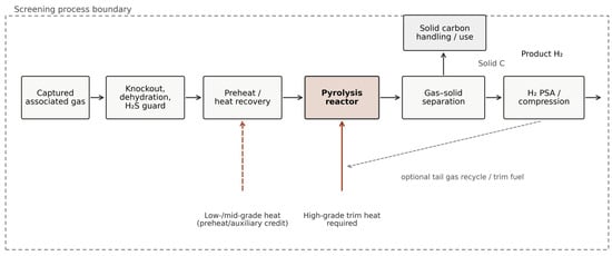
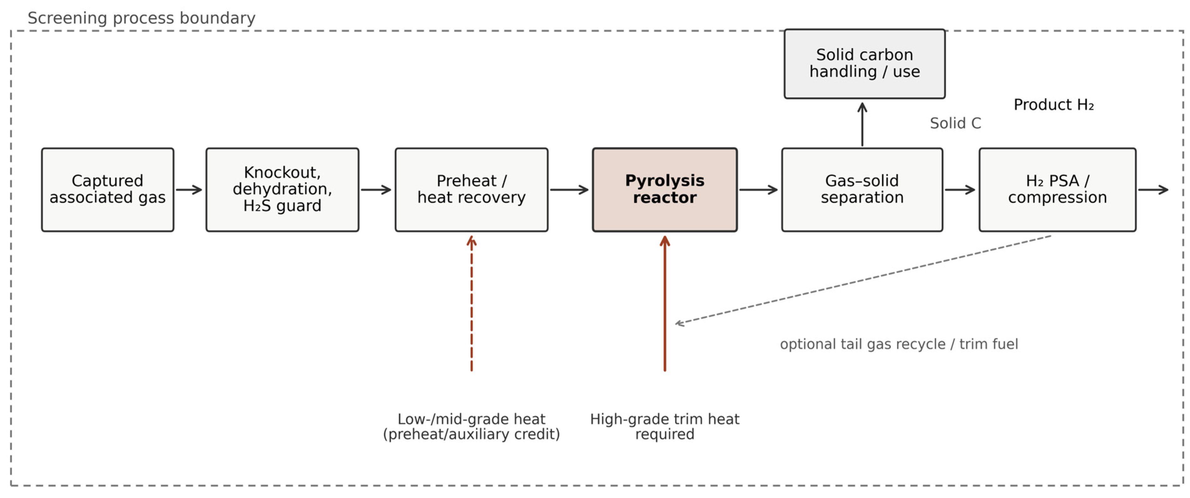
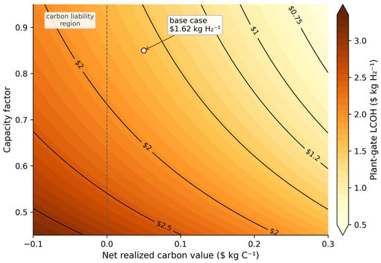
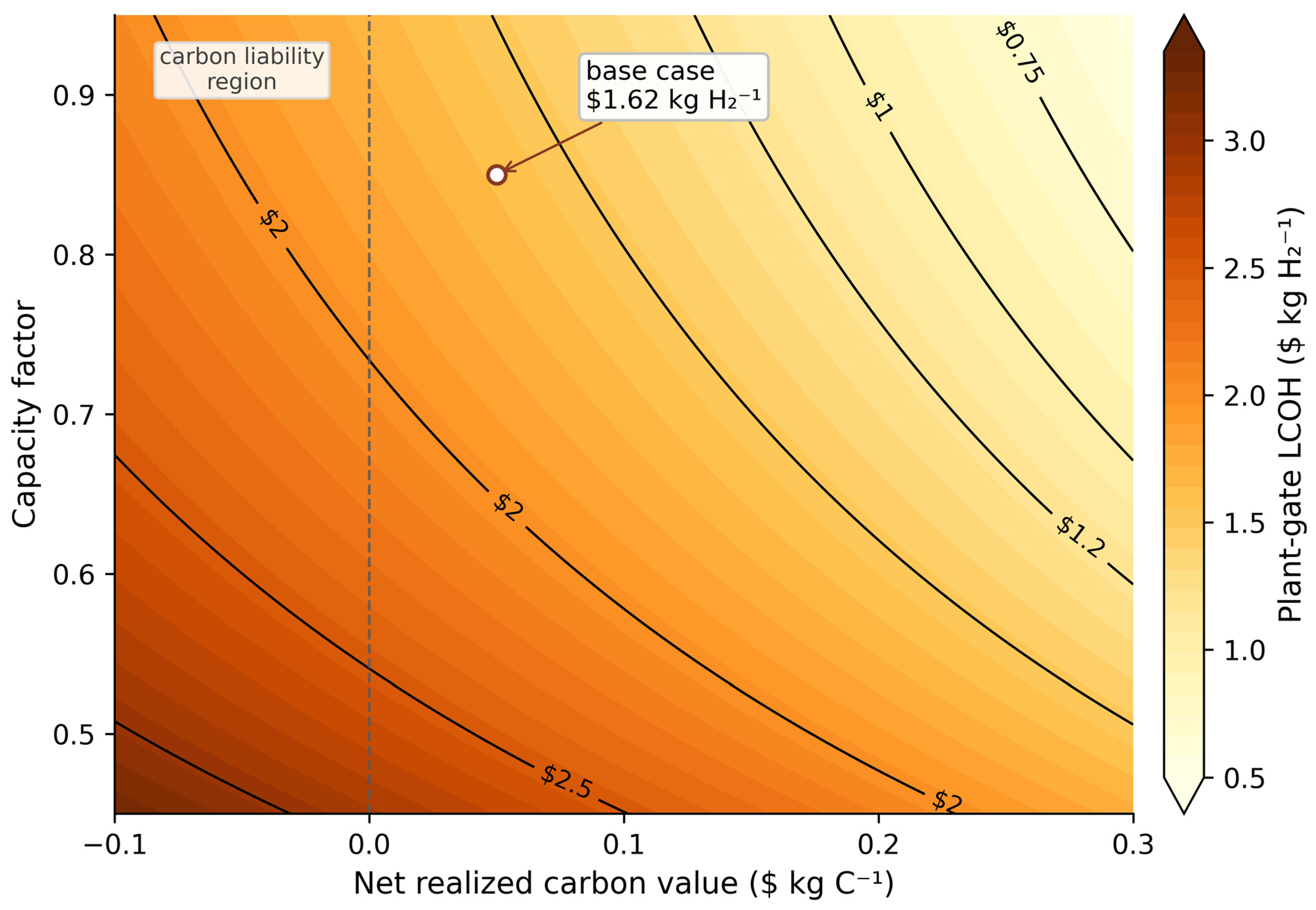
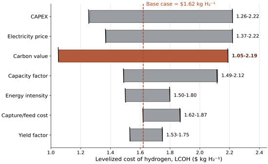
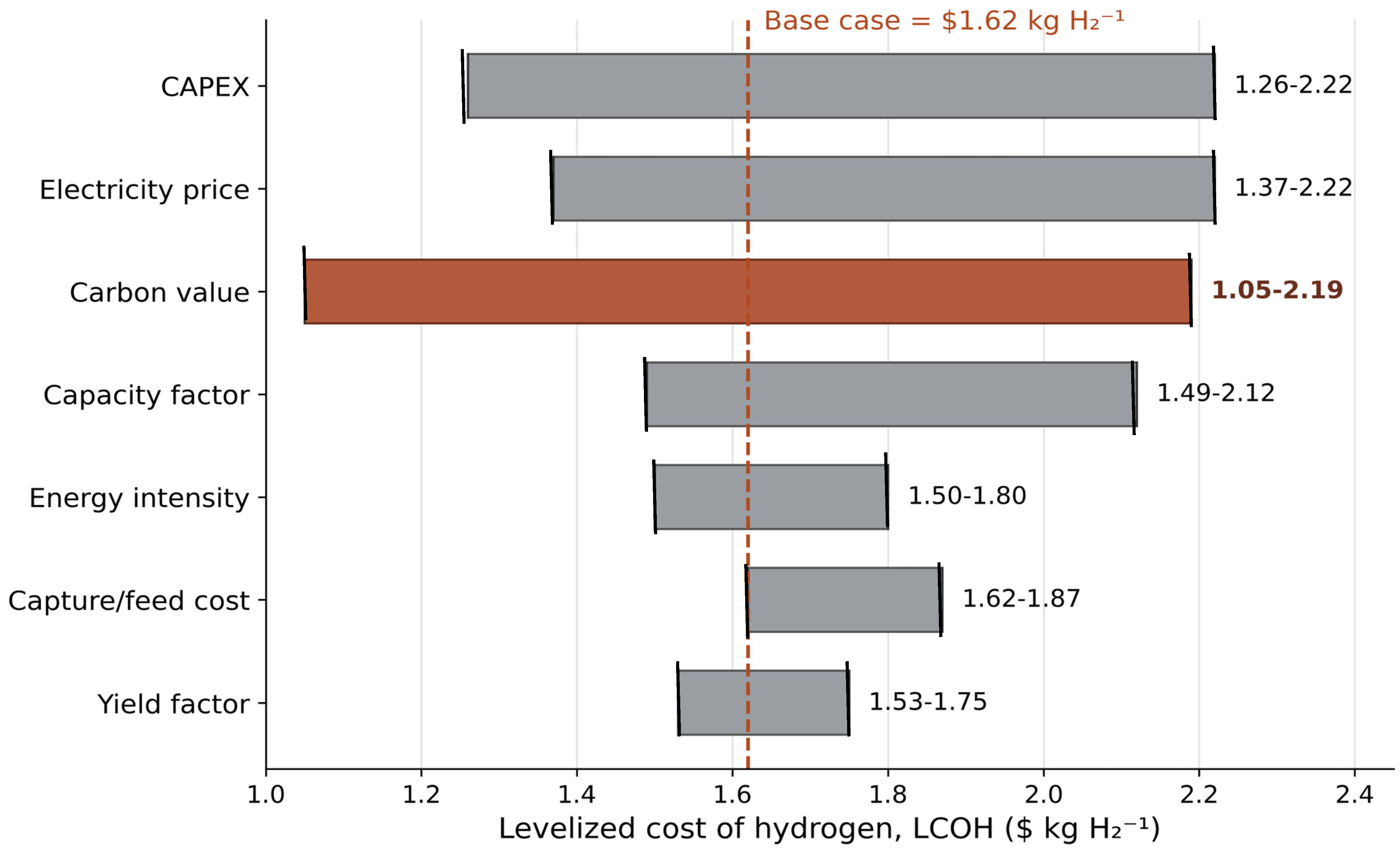
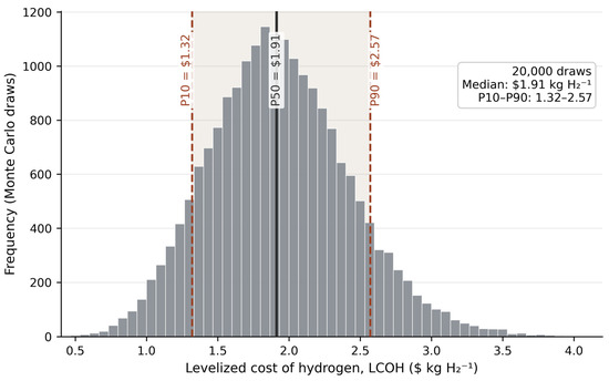
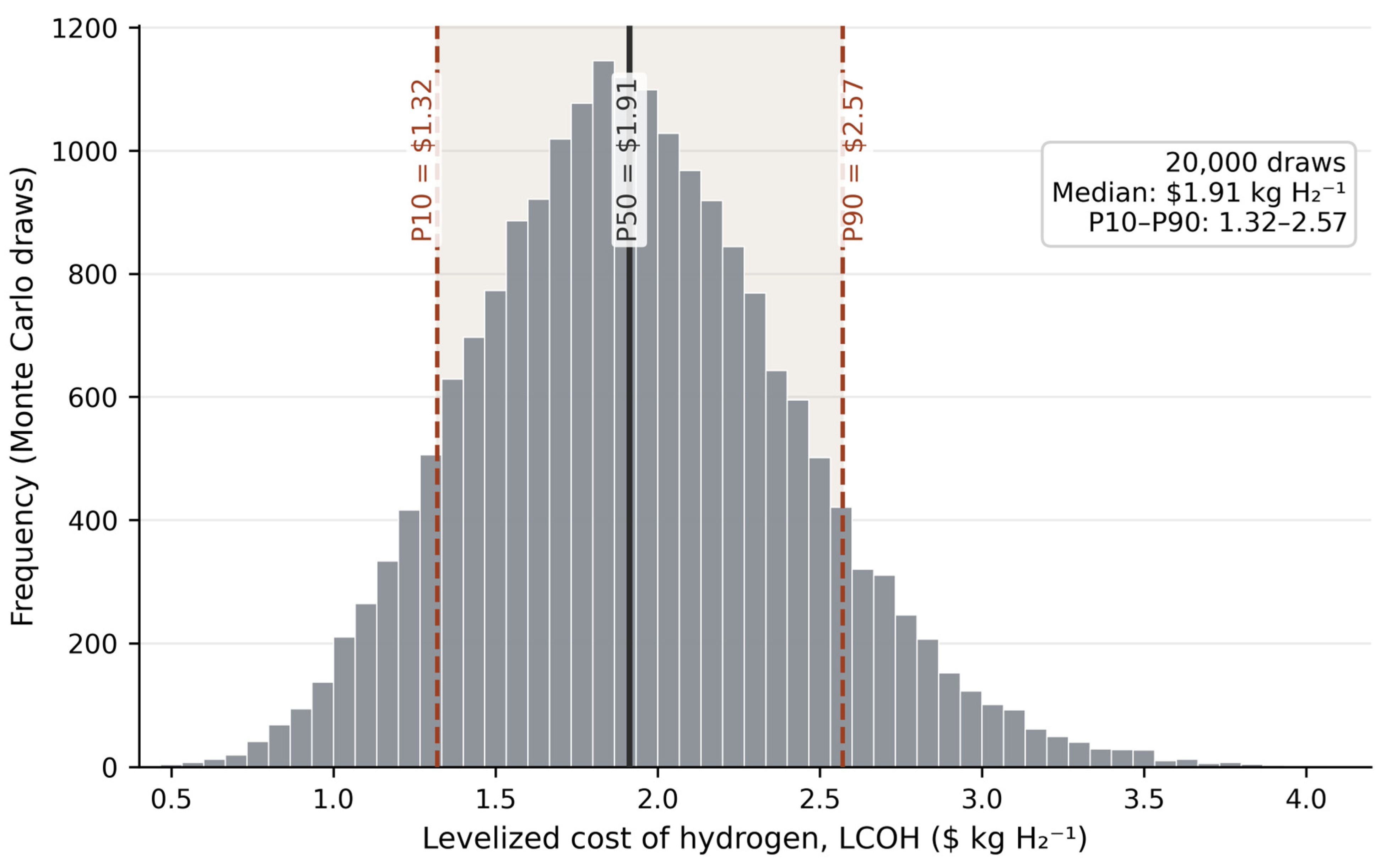
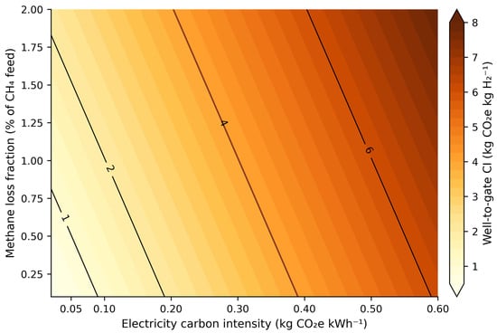
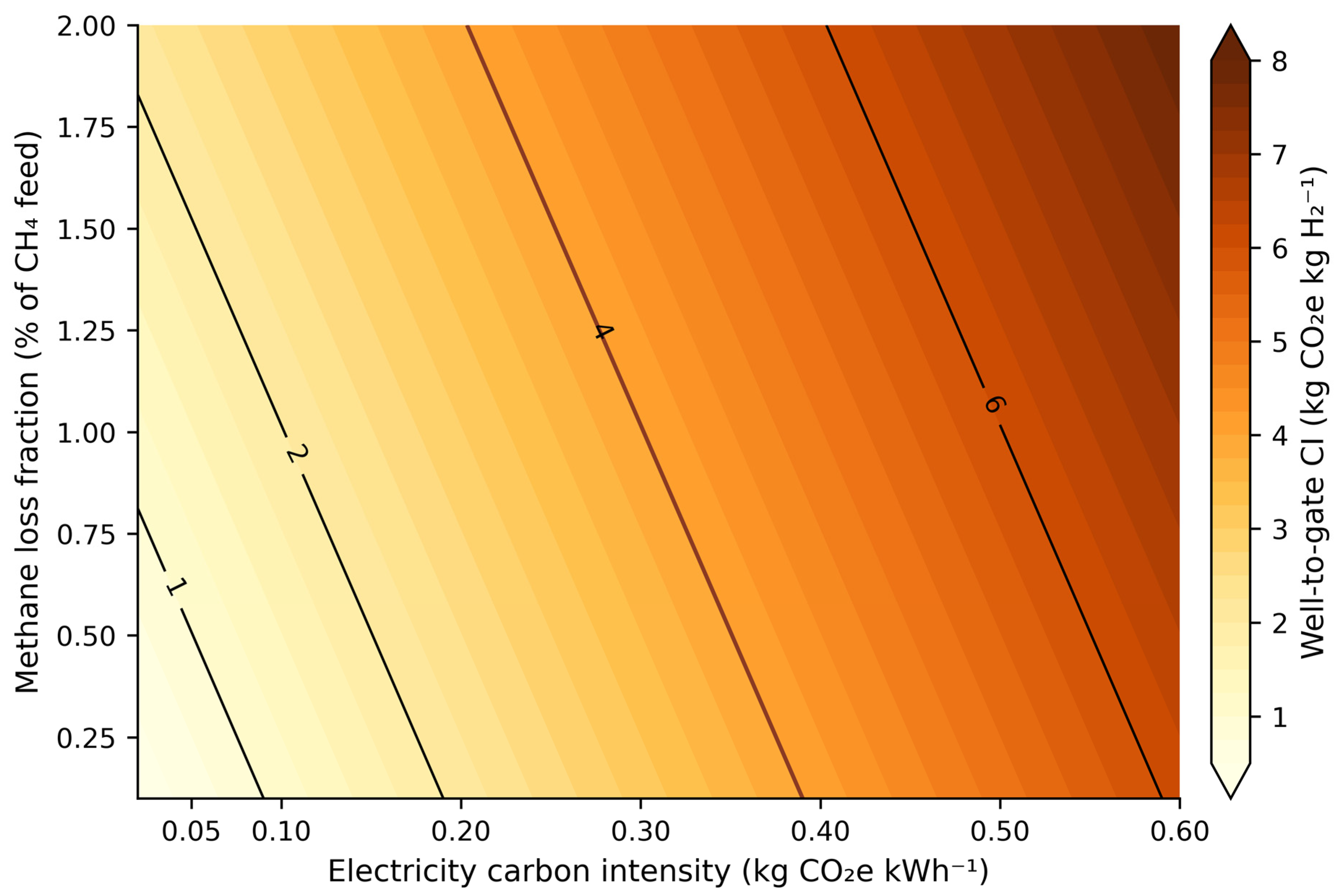
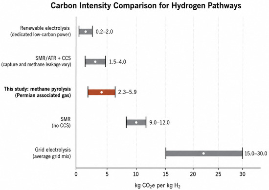
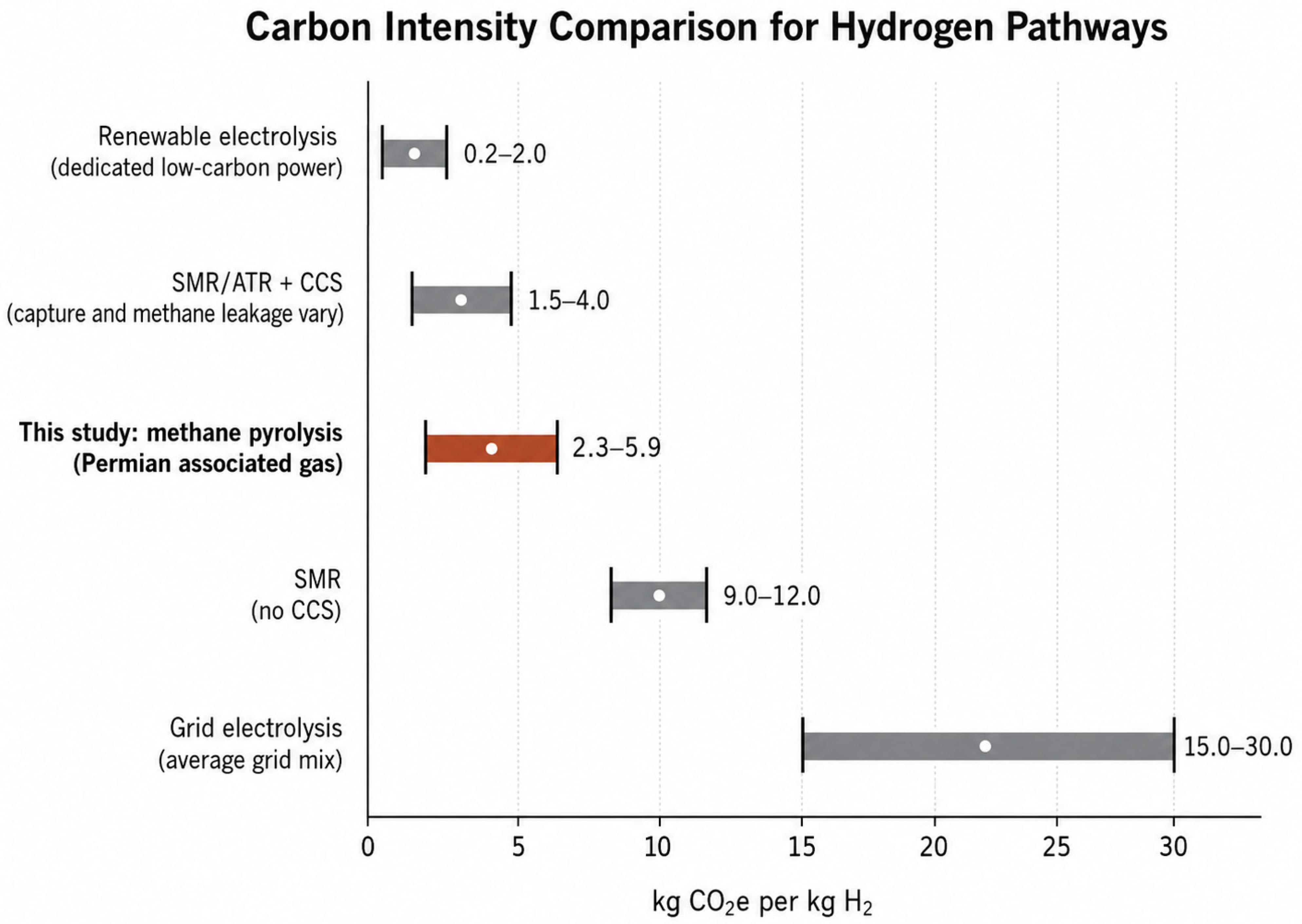

Disclaimer/Publisher’s Note: The statements, opinions and data contained in all publications are solely those of the individual author(s) and contributor(s) and not of MDPI and/or the editor(s). MDPI and/or the editor(s) disclaim responsibility for any injury to people or property resulting from any ideas, methods, instructions or products referred to in the content. |
© 2026 by the authors. Licensee MDPI, Basel, Switzerland. This article is an open access article distributed under the terms and conditions of the Creative Commons Attribution (CC BY) license.