Physically Based Strength Simulation and Multi-Objective Design of Permeable Concrete Pavement Composition for Urban Stormwater Management System

Abstract

The strength of permeable concrete pavement (PCP) decreases as porosity increases; its water permeability depends on this porosity. Using the PRISMA 2020 guidelines, 28 open-access studies (337 mixtures) were selected that reported measured porosity, strength at 28 days, and filtration coefficient. Strength was predicted by a neural network, whose loss function incorporated the relationship between strength and porosity, its monotonically decreasing trend, and physical constraints. In the test studies, R² was 0.74; when excluding one study at a time, it was 0.31 (the network without physical terms yielded 0.43 and 0.25, and linear regression yielded 0.49 and 0.45); the differences between the models are not statistically significant. The contribution of porosity to the SHAP prediction (4.9 MPa) is an order of magnitude higher than that of the water-to-cement ratio and aggregate parameters. The filtration coefficient cannot be extrapolated to new studies; it was estimated by calculating the Boltzmann lattice equations for 500 virtual samples with a correction factor of β = 0.020. Using the NSGA-II method, mixtures with strengths of 10.0–22.1 MPa, porosity of 15–26.5%, and a carbon footprint of 311–397 kg CO₂-eq/m³ were obtained. In the EPA SWMM model for a 5-hectare watershed, a surface treatment using any of these mixtures reduces peak discharge by 96–100% during storm events with a return period of 2–50 years; permeability affects the result only when k < 0.01 cm/s. The composition should be selected based on strength and carbon footprint, while hydraulic efficiency should be ensured by the surface area of the pavement and the storage capacity of the subgrade. The results were obtained through calculation and require experimental verification.

1. Introduction

Rapid urbanization and global climate change are leading to an increase in the frequency and intensity of extreme storm events, which causes critical overload of traditional urban stormwater drainage systems. In response to these challenges, the concept of “sponge cities” and low-impact development technologies offer a model for decentralized stormwater management directly at the source [1].

As a key engineering tool, permeable concrete pavements (PCPs) have proven to be an effective solution that facilitates surface water infiltration, replenishes aquifers, and reduces the “urban heat island” effect [2,3], as confirmed by review studies on the materials science and performance characteristics of PCP [4]. However, the widespread adoption of PCP is hindered by a fundamental materials science trade-off between its filtration capacity and mechanical strength. The permeability of concrete depends directly on its effective porosity, which, in turn, exponentially reduces the material’s compressive strength. This nonlinear relationship is traditionally described by the Ryshkevich equation:

fc = f₀ · exp(−b · P_c)

(1)

where f_c—compressive strength, MPa; f₀—compressive strength at zero porosity, an approximation parameter, MPa; b—empirical coefficient; and P_c—porosity, %.

Traditional approaches to designing PBP mixtures rely on empirical methods and laboratory trialanderror. This process is resource-intensive, time-consuming, and does not allow for effective exploration of the multidimensional parameter space (fractional composition of coarse aggregate, water–cement ratio, type and dosage of chemical admixtures) [5,6]. In recent years, machine learning methods have been actively used to predict concrete properties [7,8,9]. However, standard algorithms operate as “black boxes” and do not account for physical laws, which can lead to physically incorrect predictions when extrapolating beyond the training sample [10].

To overcome the limitations of the approach described, which is based on data, the scientific community is shifting toward the use of Physics-Informed Machine Learning (PIML) [11]. This approach integrates physical relationships (e.g., the relationship between strength and porosity or the condition of its monotonically decreasing behavior) directly into the neural network’s loss function [12,13].

At the same time, multi-criteria optimization (e.g., the NSGA-II algorithm) allows for the identification of Pareto-optimal compositions under several conflicting requirements [14].

However, a significant methodological gap exists in the scientific literature: most studies optimize material properties exclusively at the microscale, ignoring their integrated impact at the macroscale—namely, the hydrological response of an urban watershed when modeling storm events [13,14]. There is no unified computational pipeline linking the generation of a virtual microstructure, PIML strength prediction, and hydrological modeling (e.g., in the EPA SWMM environment) [15]. To confirm the claimed novelty, the proposed framework was compared with the three most closely related studies, which cover individual aspects of the pipeline (Table 1).

Table 1. Comparison ofthe proposed framework with the most relevant studies from 2022–2026 in terms of method, simulation level, and the presence of experimental validation.

Work	Method	Simulation Level	Experimental Validation
This work	PRISMA dataset → PIML strength (Ryshkevich formula, monotonicity, boundaries) → estimation of k(Pc) using LBM with β correction → NSGA-II within the model’s applicability domain → EPA SWMM	Multiscale: material microstructure → operational properties of the PBP → hydrological response of the watershed	None (computational, in silico modeling only)
EcoBlendNet (Rahman & Lu, 2024, J. Cleaner Production) [13]	PINN with a physical constraint on the cement hydration PDE (adiabatic heating)	Materials science, micro-scale (cement paste cell ~100 × 100 μm); no integration with coating or hydrology	Yes—calibrated using experimental data on adiabatic heating for 3 compositions
Chen et al. (2022, Cement and Concrete Composites) [14]	RF (feature selection) + LSSVM (property prediction, without physical constraints) + NSGA-II	Materials science (design of high-quality concrete mixtures; no integration with pavement or hydrology)	Available—data from a real-world project (Sunyuan–Tongyu Expressway)
Li, Xu, Hu (2026, J. Hydrologic Engineering, Vol. 31, No. 3) [15]	Calibration of SWMM using a neural network with parameters selected by a modified sparrow search algorithm; surrogate deep neural network + NSGA-II for selection of LID measures based on cost, runoff, and suspended solids	Hydrological: residential and office district (Xi’an); the composition and properties of the pavement material are not considered	SWMM calibration for a real-world site; a reduction of 85.9% in runoff and 86.1% in suspended solids was obtained through calculation

As can be seen from the comparison, each of the three studies addresses only one level of the problem: Refs. [13,14] focus on materials science (physically informed and data-driven, respectively), while ref. [15] focuses on hydrology: it optimizes the placement of LID measures in SWMM but does not link them to material composition. None of them integrates microstructure generation, physicallyinformed strength prediction, and hydrological modeling of a watershed into a single reproducible computational pipeline—it is precisely this combination, rather than the individual components, that constitutes the claimed novelty of this work.

The objective of this work is to construct a reproducible computational chain for designing the composition of the PBP (“literature data → strength model with physical constraints → permeability estimation using the LBM → multi-objective optimization → hydrological model of the watershed”) and to determine which of its links are transferable to data from new studies.

The scientific novelty of this work lies in the following:

• The strength model was evaluated by transferring it to studies not included in the training set; the physical terms of the loss function increase the neural network’s R² on test studies from 0.43 to 0.74 and, upon sequential exclusion of studies, from 0.25 to 0.31; however, based on confidence intervals, the differences between PIML, a network without physical terms, and linear regression (0.45) are statistically insignificant.
• It was established that the filtration coefficient derived from the literature data is not transferable across studies, and a method for estimating it based on LBM calculations with a constant correction factor was proposed; the absence of a trend in this factor with respect to porosity was verified statistically.
• Hydrological calculations show that, within the obtained Pareto front, the concrete composition does not affect runoff, and a permeability threshold (0.01 cm/s) has been determined, which defines the safety margin against clogging.

Limitations of the study: All quantitative results presented in this work were obtained using computational modeling methods and require subsequent experimental validation; a detailed discussion of the study’s limitations, key assumptions, and a plan for further testing is provided in Section 4.4.

2. Materials and Methods

The computational workflow consists of five stages: generating a set of experimental data according to the PRISMA guidelines; calculating the permeability of virtual samples using the LBM and scaling it to the experimental level; training and validating a strength model with physical constraints and interpreting it using the SHAP method; multi-objective optimization of the composition; and simulation of runoff in EPA SWMM. Verification of the LBM solver, data partitioning, and calculation of the correction factor were performed in MATLAB R2025b; the calculation of 500 LBM samples was carried out using the same procedure in Python 3 with Numba compilation (on the test problem, both implementations match to the fourth decimal place). The strength model, SHAP, NSGA-II, and SWMM scenarios were implemented in Python 3.14.8 (PyTorch, scikit-learn, swmm-toolkit).

2.1. Dataset Creation and Permeability Calculation Using the LBM

2.1.1. Systematic Literature Review and Data Structuring

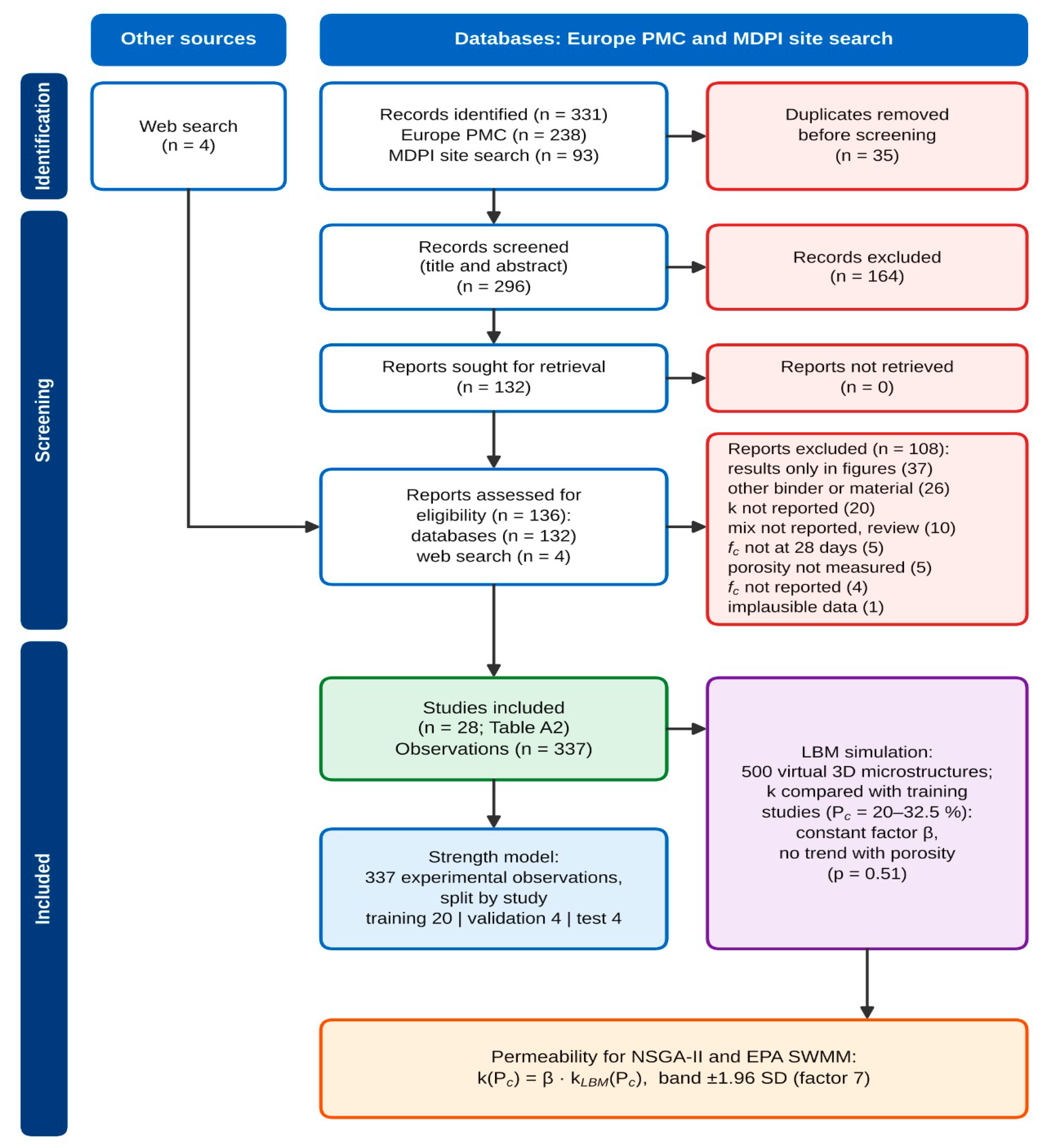
Experimental data were collected through a systematic search of open-access publications following the PRISMA 2020 guidelines [16] (Figure A1); the search was conducted on 7 October 2026. In Europe PMC, the following query was used: (“pervious concrete” OR “porous concrete” OR “permeable concrete” OR “no-fines concrete”) AND (permeability OR “hydraulic conductivity”) AND (porosity OR “void ratio” OR “void content”) AND “compressive strength,” restricted to open-access full text (238 records). A search on the MDPI website yielded an additional 93 records, and a general web search found 4 studies. After removing 35 duplicates based on title and abstract, 296 records were reviewed. The full text was evaluated for 136 studies: 132 from databases and 4 from the web search.

We included studies on permeable concrete made with Portland cement in which the water–cement ratio (W/C), aggregate dosage or maximum aggregate size, measured porosity, compressive strength at 28 days, and filtration coefficient were specified for each mixture. The filtration coefficient is included in the inclusion criteria, although the model predicts only strength: the measured values of k were used to calibrate the correction factor β of the LBM model (Section 2.1.2).

In total, 108 studies were excluded for the following reasons:

• Results presented only in graphs—37;
• Different binder or material—26;
• Filtration coefficient not determined—20;
• The composition of each mixture was not provided, or the study was a review—10;
• Strength was not determined at 28 days—5;
• Porosity was not measured—5;
• Strength not determined—4;
• Unreliable data—1.

The final dataset included 337 observations from 28 studies conducted between 2017 and 2026 [17,18,19,20,21,22,23,24,25,26,27,28,29,30,31,32,33,34,35,36,37,38,39,40,41,42,43,44]. The list of studies, the number of compositions, and their assignment to samples are presented in Table A2.

Only values listed in tables or in the text for a specific composition were included in the dataset; data from graphs were not digitized. Each value of fc, Pc, and k was cross-checked against the full text of the source. If both total and effective porosity were reported, the effective porosity was used; the filtration coefficient was converted to cm/s. For each observation in the dataset, the shape and size of the sample are specified (100- and 150-mm cubes—134 observations; 100 × 200, 104 × 208, and 150 × 300-mm cylinders—68; other or unspecified—135), the method used to determine the filtration coefficient (variable head—95, constant head—74, other or unspecified—168), and the method used to determine porosity. The strength of samples of different shapes relative to the reference standard was not recalculated. The microsilica content is expressed relative to the binder mass; nanosilica [41] and microsilica as part of a composite additive [34] are accounted for in the same variable as an active silica-based additive. In 78 observations from 7 studies, only one of the two aggregate parameters was specified: the dosage was not specified in 57 observations, and the maximum particle size was not specified in 21. Missing values were replaced with the median of the training sample. The characteristics were standardized using the mean and standard deviation of the training sample. The dataset, the selection log with reasons for exclusion, and the value carryover tables are available in the repository.

The division into training, validation, and test sets was performed at the study level: all observations from a single study were assigned to a single set. Observations from a single study were obtained using the same equipment, from the same batch of materials, and following the same testing methodology. If they had been included in both the training and test sets simultaneously, the model might have captured the characteristics of the laboratory rather than the dependence of strength on composition, and the accuracy metrics (Table 2) would have been overestimated. For the same reason, publications by a single research team were placed in a single set. Of the 28 studies, 20 were assigned to the training set (236 observations), 4 to the validation set (51), and 4 to the test set (50), corresponding to a ratio of 70/15/15%.

Table 2. Accuracy of strength prediction on the test sample (4 studies, 50 observations) and when excluding one study at a time (28 studies, 337 observations).

Model	Test: R2	RMSE, MPa	MAE, MPa	Across Studies: R2	RMSE, MPa	MAE, MPa
PIML	0.742	3.99	3.34	0.311	6.94	5.03
DNN	0.430	5.92	4.83	0.249	7.25	5.33
Formula (1)	0.696	4.32	3.72	0.303	6.98	5.24
Linear regression	0.494	5.59	4.38	0.448	6.21	4.82
SVR	0.131	7.32	6.03	0.073	8.05	6.00
XGBoost	0.557	5.23	4.21	0.317	6.91	5.38
LightGBM	0.440	5.87	4.68	0.286	7.07	5.51

2.1.2. Numerical Simulation of Microstructure (LBM)

The Lattice Boltzmann Method (LBM) was used to estimate the filtration coefficient. This method allows for the calculation of flow directly within the pore space of a given geometry [45].

The calculation included the following steps:

• Construction of microstructures. A total of 500 virtual samples of permeable concrete with dimensions of 100 × 100 × 100 voxels were generated. Spherical aggregate grains with a nominal diameter d_agg ranging from 5 to 20 mm (±20% variation) were placed using the random sequential addition (RSA) method, starting with the largest grains. The centers of the grains were distributed within a region extended by the grain radius to prevent the formation of a sparse layer at the sample boundaries. Then, using morphological dilation, a cement paste shell with a thickness ranging from 0.25 to 0.50 times the grain radius—but no less than one voxel—was applied to the grains. The volume fraction of aggregate ranged from 0.31 to 0.42, and the porosity of the samples ranged from 7.8 to 48.1% (median 23.5%). For identical spheres, random sequential packing reaches saturation at a volume fraction of approximately 0.38 [46]; higher values were obtained due to the spread of diameters, while lower values correspond to large grains, of which there are few in the computational domain. This fraction is lower than in real permeable concrete; therefore, the required solid-phase content is provided by the cement paste shell, which corresponds to the material’s structure. The porosity range of the virtual samples covers the experimental range (6.3–36.5%), with the exception of 7 mixtures with porosity below 7.8%.
  A voxel size of 0.5 mm (with a computational domain side length of 50 mm) was chosen as a compromise between the resolution of the pore channels and the size of the domain. The characteristic pore size of permeable concrete is 1.5–5 mm [47]; therefore, the pore diameter corresponds to 3 to 10 lattice nodes. Based on the power-law relationship between the error and resolution, |εκ| ≈ 0.6·B^(–1.6), where B is the number of nodes per channel diameter [48], the error in determining permeability ranges from 1.5 to 10%. The edge of the region is equal to 2.5 times the nominal diameter of the largest aggregate (20 mm), and, taking into account the size distribution, 2.1 times the diameter of the largest grain. Therefore, for mixtures with d_agg > 15 mm, LBM results should be considered approximate.
• Flow calculation. The discrete LBM equation takes the form:

  f_i(x + c_i Δt,t + Δt) − f_i(x,t) = −1/τ [f_i (x,t) − f_i^eq(x,t)]

  where f_i is the distribution function in the i-direction, c_i is the velocity vector, f_i^eq is the equilibrium distribution function, τ is the relaxation time, and Δt is the time step.
  A D3Q19 grid with a single relaxation time (BGK) was used, as in [49], where the permeability of the reconstructed permeable concrete was calculated for a domain of 100 × 100 × 100 nodes. We set τ = 1.0, which yields a kinematic viscosity in grid units of ν = (τ − 0.5)/3 = 1/6 [50]. In the range 0.5 < τ ≤ 1.0, the error of the BGK scheme with bounce-back reflection remains acceptable [51]; when τ > 1, the calculated permeability begins to depend on viscosity [52]. Boundary conditions:

  –

  At the solid-phase surface: bounce-back reflection;

  –

  At the inlet and outlet faces–constant pressure according to the Zou–He scheme [53], with a density ratio ρin/ρout = 1.001;

  –

  The side faces are impermeable, as in [49];

  –

  Three layers of free liquid were added in front of the inlet face and behind the outlet face [51].

  The pressure drop was determined based on cross-sections at the sample boundaries, rather than on the buffer layers [48]. The calculation was terminated when the relative change in the sample-averaged filtration rate over 1000 steps became less than 5 × 10⁻⁴ (maximum number of steps—30,000). The residual error k under this criterion is comparable to 0.05%. Convergence required between 2000 and 29,000 steps (median: 4000). The Mach number did not exceed 1.7 × 10⁻³ in any of the calculations; therefore, the compressibility of the grid fluid can be neglected [50]. The pore Reynolds number was below 0.1, meaning the flow remained within the applicability range of Darcy’s law. The flow rate imbalance between the inlet and outlet did not exceed 1%. The solver was tested on flow in a square-cross-section channel: the deviation from the exact solution was 0.37% for a 20 × 20 grid. Simulations without a connected pore cluster in the flow direction that did not meet the convergence criterion or had a flow imbalance of more than 1% were replaced with a new mesh configuration using a different generator seed; there were 42 such simulations. A complete list of parameters is provided in Appendix A (Table A1).
• Calculation of permeability. The permeability κ, m², was calculated using Darcy’s law based on the steady-state filtration rate at a given pressure gradient ∇P:

  k = −μ⟨u⟩/∇P

  where μ is the dynamic viscosity; ⟨u⟩ is the filtration rate averaged over the entire volume of the sample, including the solid phase. The filtration coefficient was calculated as k = κρg/μ for ρ = 998 kg/m³ and μ = 1.0 × 10⁻³ Pa·s (water, 20 °C) and was expressed in cm/s, as were the experimental data. Each of the 500 microstructures yielded one pair of “porosity–filtration coefficient” values. Porosity was determined by counting the pore voxels.
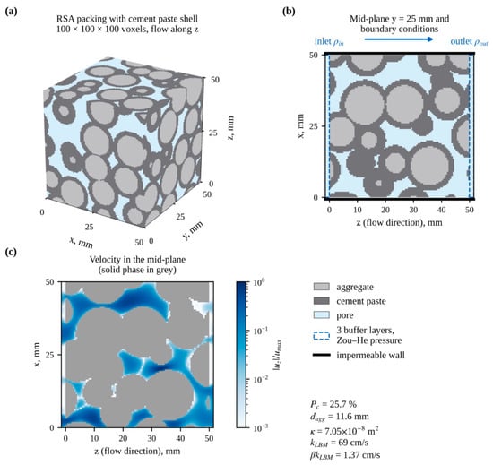
• Comparison with Experiment. The calculated values of k were compared with experimental data from 20 studies in the training sample across the entire porosity range. The range of 20–35% was divided into intervals 2.5% wide. In each interval containing at least five experimental and five calculated data points, the difference between the mean logarithms ln k_exp − ln k_LBM was calculated. Five intervals (20–32.5%) satisfied this condition. LBM overestimates the filtration coefficient: the average ratio k_exp/k_LBM was β = 0.020 (95% CI 0.012–0.032, bootstrap across studies). The slope of the relationship ln(k_exp/k_LBM) versus porosity is insignificant (0.022 per 1%, p = 0.51). Consequently, LBM captures the shape of the k(P_c) relationship, while the discrepancy in magnitude is constant. The calculated values of k are multiplied by β; the original values are retained in the dataset as a separate column. The calculation sequence is shown in Figure 1.
  

  Figure 1. Permeability calculation using the LBM on a virtual sample (P_c = 25.7%, d_agg = 11.6 mm): (a)—packing of aggregate grains with a cement stone shell (100 × 100 × 100 voxels, 50 × 50 × 50 mm); (b)—cross-section and boundary conditions; (c)—relative filtration velocity in the same cross-section. For this specimen, κ = 7.05 × 10⁻⁸ m², k = 69 cm/s; after multiplication by β = 0.020, the result is 1.37 cm/s.

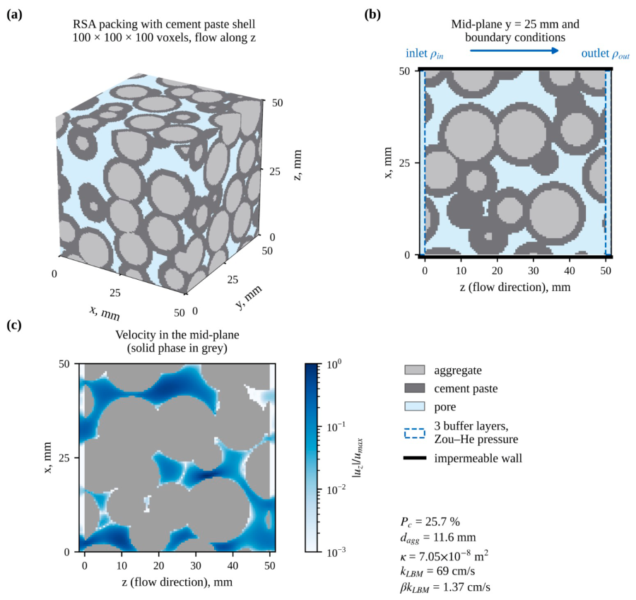
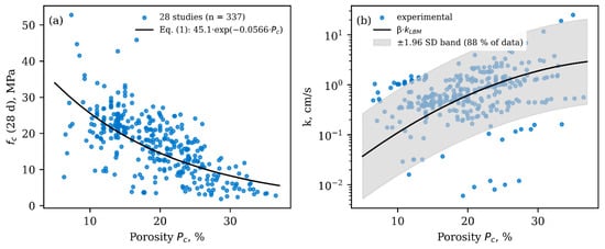
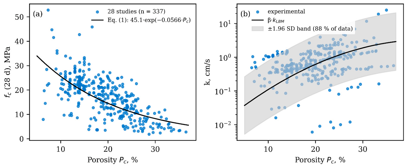
The corrected relationship log₁₀k = −0.00130·P_c² + 0.1137·P_c − 1.967 (k in cm/s, P_c in %) is used as an estimate of the filtration coefficient in Section 2.3 and Section 2.4. The standard deviation of the experimental values from the training studies relative to this relationship is 0.435 in decimal logarithms. The ±1.96 standard deviation band corresponds to a deviation from the mean of between 1/7 and 7 times the mean and covers 88% of the experimental data points (Figure 2b). Calculated data were not included in the training of the strength model.

Figure 2. Compressive strength at 28 days (a) and filtration coefficient (b) as a function of porosity: data points—337 compositions from 28 studies; the line in panel (a)—Equation (1) based on the training studies; the line and gray band in panel (b)—the LBM dependence normalized to the experimental level by the factor β, and its uncertainty band (±1.96 standard deviation).

2.2. Strength Model

2.2.1. Problem Statement and Comparative Models

The model’s output is the compressive strength at 28 days, f_c; the inputs are the water-to-cement ratio (W/C), the mass fraction of coarse aggregate in the dry components, the mass fraction of microsilica in the binder, the porosity P_(c), and the maximum aggregate size. The filtration coefficient was not predicted by machine learning: when tested with out-of-sample data, none of the models (gradient boosting, linear regression, the Kozhen–Karmann formula) predicted log₁₀k for the new test data better than their mean value (R² < 0). The discrepancy is attributed to differences in measurement methods between laboratories (constant and variable pressure, sample size, porosity determination) rather than to the composition of the mixture.

We compared a physics-informed neural network (PIML), the same network without physics-based terms (DNN), Formula (1), linear regression, radial basis SVR, XGBoost, and LightGBM. Performance was evaluated in two ways: on a test set consisting of 4 studies (50 observations) and by sequentially excluding each of the 28 studies (leave-one-study-out). Metrics used were R², RMSE, and MAE.

2.2.2. Physically Informed Loss Function

All models are implemented in Python 3.13. The PIML model and the network without physical terms are written in PyTorch 2.14; the parameters of Equation (1) were estimated using the least-squares method for ln fc (NumPy 2.5). Linear regression and SVR were implemented using scikit-learn 1.9, while gradient boosting was implemented using the XGBoost 3.4 and LightGBM 4.7 libraries. For linear regression and SVR, the inputs were standardized based on the training set; SVR parameters: C = 30, ε = 0.5. The XGBoost and LightGBM models each contained 400 trees with a learning rate of 0.03. The parameters of the base models were set in advance and were not tuned. Metrics and the study exclusion procedure were calculated using custom code (NumPy, pandas).

L = L_data + λ_R ·L_R + λ_M·L_M + λ_BL_B

(2)

where L_data is the root-mean-square error based on experimental data; L_R is the deviation of the prediction from Equation (1), whose parameters (f₀ = 45.06 MPa, b = 0.0566) were determined from training experiments (Figure 2a); L_M is the penalty for a positive derivative ∂f_c/∂P_c, calculated by automatic differentiation; and L_B is the penalty for the prediction falling outside the range of 0–70 MPa. The physical terms are computed at collocation points that uniformly cover the training data region with a 10% margin, rather than only at the data points. The architecture (32–16 neurons, tanh), learning rate (10⁻³), and λ_R = 3 were selected based on validation studies from among 12 options; λ_M = λ_B = 1. Training—Adam [54], batch size 64, no more than 1500 epochs with early stopping if the error on the validation set does not decrease for 100 epochs; at each step, the physical terms are computed at 256 random collocation points. For λ_R = 0.3, 1, and 3, R² on the validation set was 0.44, 0.52, and 0.53, respectively. A network without physical terms (DNN, λ_R = λ_M = λ_B = 0) serves as an ablation comparison. The forecast is the average of five networks with different initializations.

2.2.3. Interpretation (SHAP)

The contribution of inputs to the PIML prediction is estimated using Shepley values [55], calculated by the permutation sampling method [56]. Threshold values were determined using a two-segment piecewise-linear regression of the SHAP value as a function of the variable. The significance of the break was tested using the F-test against a linear relationship, and the confidence interval for the break point was determined using bootstrapping (300 repetitions).

2.3. Multi-Objective Optimization (MOO)

2.3.1. Formalization of Objective Functions

The mix design is formulated as a multi-objective optimization problem using the PIML strength model. The vector of design variables x includes the water-to-cement ratio, the coarse aggregate content, the microsilica content, and the porosity P_c.

The optimization aims to simultaneously achieve three conflicting objectives:

• Maximizing porosity F₁(x) = max P_c, which determines the coating’s capacity and, via the relationship in Section 2.1.2, its water permeability.
• Maximizing structural integrity: F₂(x) = max(f_c(x)), where f_c is the compressive strength, MPa.
• Minimization of environmental impact: F₃(x) = min(GWP(x)), where GWP is the global warming potential (carbon footprint), kg CO₂-eq/m³, calculated based on the emission factors of the mixture’s ingredients (cement, aggregates, admixtures) [57].

The component consumption per 1 m³ was determined using the absolute volume method based on the water-to-cement ratio, the aggregate content, the microsilica content, and the porosity P_c, assuming a density of 3150 kg/m³ for Portland cement, 2200 kg/m³ for microsilica, 2650 kg/m³ for aggregate, and 1000 kg/m³ for water. Emission factors (stages A1–A3) are based on ICE v3.0 [58], kg CO₂-eq/kg: Portland cement 0.900; aggregate 0.005; water 0.0003; for microsilica as a byproduct −0.014.

Constraints: fc ≥ 10 MPa (pedestrian pavements, ACI 522R-10 [59]); Pc ≥ 15%. The variables are constrained to the 5–95th percentile range of the training data: W/C 0.22–0.35, aggregate content 71.8–81.9%, microsilica 0–8.3%, P_c 15–29.5%; the aggregate size was set at 9.5 mm. Additionally, it was required that the average distance to the five nearest training compositions in the normalized input space not exceed the 95th percentile of this distance within the training sample. This prevents the optimizer from venturing into regions where the model is not supported by data.

2.3.2. NSGA-II Algorithm

The NSGA-II algorithm [60] was used, with limited dominance, simulated binary crossover, and polynomial mutation (population of 200, 200 generations). The optimization was repeated 30 times with different initial generator numbers. Set A consists of the solution with the highest strength, Set B consists of the solution with the highest porosity for f_c ≥ 10 MPa, and Set C consists of the solution closest to the ideal point in the normalized objective space for f_c ≥ 15 MPa.

2.4. Integration with a Hydrological Model (SWMM)

The hydrological effect was evaluated using EPA SWMM 5.2 [61] (Python interface swmm-toolkit). The pavement was modeled using the Permeable Pavement module, whose performance was verified in [62]. A 150-mm-thick concrete layer has a void ratio P_c/(1 − P_c) and a permeability of k × 36,000 mm/h, where k is the value from Section 2.1.2 for the material’s porosity (cm/s). The calculation was performed for the central estimate of k and for the lower bound of its uncertainty interval (±1.96 standard deviation). A 300-mm-thick crushed-stone base has a void ratio of 0.40 (porosity of 0.29), infiltration into the underlying soil is 5 mm/h, there is no drainage, and clogging was not modeled.

The 5-hectare catchment area consists of 60% impervious surfaces; infiltration in permeable areas is described by the Horton model (76.2 → 12.7 mm/h). The watershed is 200 m wide with a 1% slope; the Manning roughness coefficient is 0.012 for impervious surfaces and 0.15 for permeable surfaces, with depression retention of 2 and 5 mm, respectively (for 25% impervious area—no retention); the pavement surface has no curb, a roughness coefficient of 0.015, and a slope of 1%. In the baseline scenario, impervious surfaces are made of asphalt. In scenarios with PBP, 1.5 ha of impervious area are replaced with permeable pavement, which also receives runoff from the remaining 1.5 ha of impervious surfaces (area ratio 1:1).

The design storm events are not tied to a specific city. The intensity was determined using the formula in SN RK 4.01-03-2011 [63]:

q = q₂₀ · 20ⁿ · (1 + lg P/lg m_r)^γ/tⁿ

(3)

where q is the average rainfall intensity over a duration of t, L/(s·ha);

t—the duration of the rainfall, min; q₂₀—rainfall intensity over a 20-min period with a return period of P = 1 year, L/(s·ha); P—return period of the design intensity (recurrence interval), years; n, γ—exponents; and m_r—average number of rainfall events per year.

Values typical of a temperate continental climate are used: q₂₀ = 80 L/(s·ha), n = 0.71, m_r = 150, γ = 1.54. The intensity is converted to mm/h using the ratio 1 L/(s·ha) = 0.36 mm/h; the precipitation layer over time t is equal to q·t.

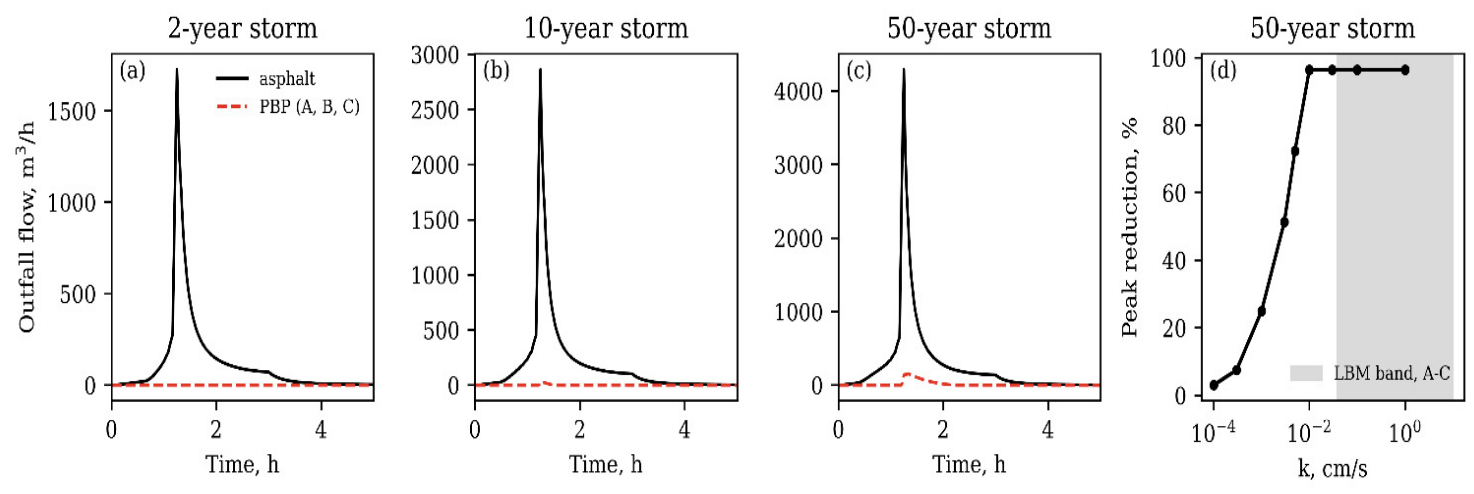
Histograms covering a 3-h duration with 5-min intervals were constructed using the alternating blocks method [64], with a peak at 40% of the duration for return periods of 2, 10, and 50 years. The precipitation depth was 22.2; 32.5, and 44.2 mm, respectively, and the maximum 5-min intensity was 94, 138, and 187 mm/h. Additionally, for the 50-year storm, permeability ranged from 1 to 10⁻⁴ cm/s. The runoff balance error in all calculations does not exceed 0.15%.

3. Results

3.1. Accuracy and Reliability of ML Models

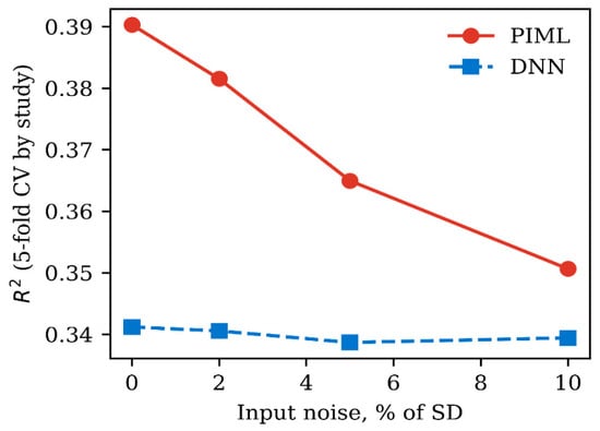
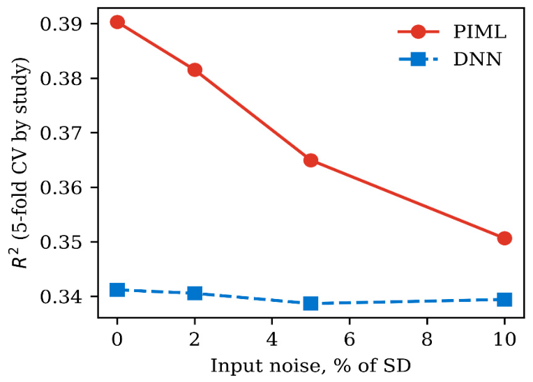
On the test set, PIML yielded R² = 0.742 (RMSE 3.99 MPa, MAE 3.34 MPa), the network without physical terms yielded R² = 0.430, the formula (1)—0.696, XGBoost—0.557, linear regression—0.494, LightGBM—0.440, and SVR—0.131 (Table 2). When excluding one study at a time, the values are lower: PIML—0.311, Formula (1)—0.303, XGBoost—0.317, DNN—0.249, and linear regression—0.448. Physical terms reduce the neural network’s transfer error to new studies but do not provide an advantage over a simple linear model: a significant portion of the strength variation (MAE 5 MPa) is determined by differences between laboratories that are not reflected in the input variables. With input noise up to 10% of R², the PIML in a 5-fold group cross-validation decreased from 0.39 to 0.35, while the DNN remained at 0.34 (Figure 3). Outside the data range, none of the networks produced negative strength or an increase in strength with porosity.

Figure 3. Coefficient of determination for strength prediction in 5-fold group cross-validation (28 studies) with noise in the training sample’s input data ranging from 0–10% of the standard deviation: PIML and the same network without physical terms (DNN).

Confidence intervals for R² when excluding one study at a time (study-based bootstrap, 2000 repetitions): PIML 0.06–0.57, DNN −0.03…0.48, linear regression 0.08–0.66, XGBoost 0.08–0.46. The difference in R² between PIML and DNN is 0.06 (95% CI −0.04…0.17), and between PIML and linear regression is −0.14 (−0.46…0.16); that is, the differences between the models are statistically insignificant. The test sample consisting of four studies does not allow for the estimation of a confidence interval; therefore, R² = 0.74 characterizes only these studies. Five-fold cross-validation (Figure 3) was performed by grouping the studies.

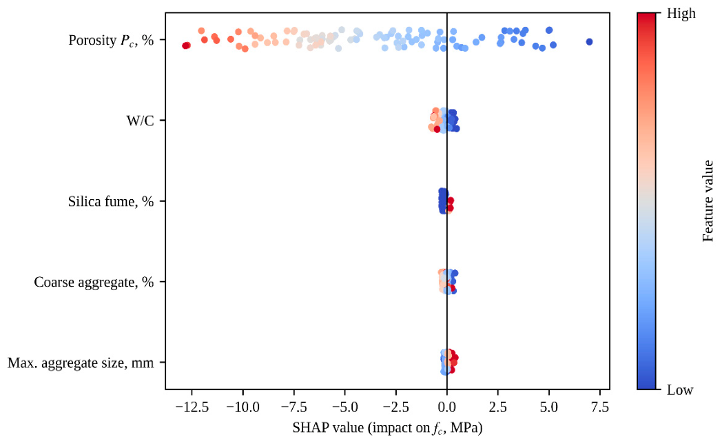
3.2. Contribution of Variables to Strength Prediction (SHAP)

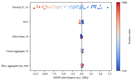
Porosity is the determining factor for strength: average |SHAP| = 4.90 MPa (95% CI 4.29–5.57). The contributions of the other variables are an order of magnitude smaller: water-to-cement ratio—0.24 MPa, microsilica—0.16, aggregate content—0.10, and particle size—0.09 MPa (Figure 4). The small contribution of microsilica is partly due to the fact that it is present in only 6 out of 101 observations used to calculate the SHAP values; the effect of this additive on strength has not been assessed based on these data. The relationship between SHAP and porosity exhibits a break at P_c ≈ 24% (95% CI 23.1–27.5%): above this value, the decrease in strength with increasing porosity accelerates. The breaks in the W/C ratio (0.34; 95% CI 0.26–0.35), the aggregate content (81.8%; 80.5–82.3%) and aggregate size (12.5 mm; 10.0–15.9 mm) are statistically significant (p < 10⁻⁵), but correspond to a change in the prediction of less than 0.3 MPa and are of no practical significance.

Figure 4. SHAP values for strength prediction using the PIML model (101 observations from the validation and test sets); point color indicates variable values ranging from low (blue) to high (red).

3.3. Pareto-Optimal Solutions (MOO Results)

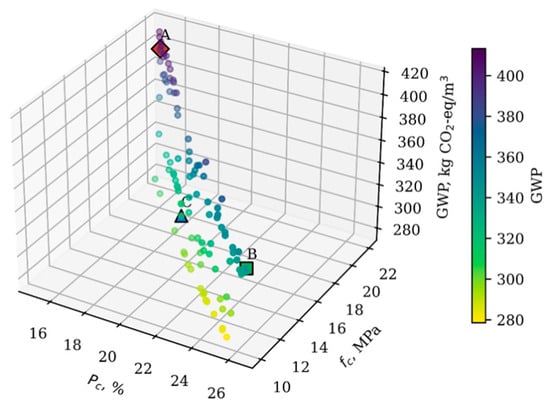
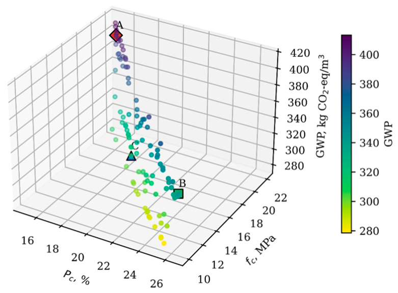
An increase in porosity from 15% to 26.5% reduces strength from 22 to 10 MPa (Figure 5). The carbon footprint of the front solutions ranges from 279 to 413 kg CO₂-eq/m³ and is determined by cement consumption. The lowest values (279–311 kg CO₂-eq/m³, 23 out of 100 solutions) were obtained at strengths of 10.0–17.3 MPa and cement consumption of 301–336 kg/m³; in half of these solutions, the W/C ratio is not lower than 0.33. Composition C was not selected based on the minimum carbon footprint, but rather as a compromise solution closest to the ideal point at f_c ≥ 15 MPa. At the same strength on the front, there is a solution with a carbon footprint of 303 kg CO₂-eq/m³ (3% lower than that of C), which differs from C mainly in its higher W/C ratio (0.34 instead of 0.26).

Figure 5. Pareto front of permeable concrete mixtures (first of 30 NSGA-II runs); color indicates carbon footprint; diamond, square, and triangle denote mixtures A, B, and C from Table 3.

The optimal permeable concrete mixtures and their predicted performance characteristics are presented in Table 3.

Table 3. Mix designs A, B, and C selected from the NSGA-II Pareto front.

Mix	W/C	Aggregate, %	Micro-Silica, %	Pc, %	fc, MPa	k (LBM), cm/s [Uncertainty Interval (±1.96 Standard Deviation)]	GWP, kg CO2-eq/m3	Cement, kg/m3
A	0.23	77.2	6.8	15.0	22.1	0.28 [0.04–2.0]	397	431
B	0.24	76.6	8.2	26.5	10.0	1.36 [0.19–9.7]	343	373
C	0.26	81.9	4.1	19.7	15.8	0.59 [0.08–4.2]	311	336

Note: The coefficient of variation for the parameters across 30 optimization runs does not exceed 4.4%, except for the microsilica content in compositions B (5.9%) and C (13.4%).

The optimization variables (W/C ratio, aggregate content, microsilica content, and porosity) unambiguously determine the consumption of the components: the total absolute volume of cement, microsilica, aggregate, and water is equal to 1 − P_c (Section 2.3.1). The consumption of components is shown in Table 4, and the carbon footprint calculated based on it is shown in Table 3.

Table 4. Component consumption per 1 m³ of concrete for mixtures A, B, and C.

Mix	Cement, kg/m3	Microsilica, kg/m3	Aggregate, kg/m3	Water, kg/m3
A	431	31	1570	106
B	373	33	1333	99
C	336	14	1583	92

Composition A was obtained with the lowest permissible water-to-cement ratio (0.23) and porosity (15%) and contains 431 kg/m³ of cement, which accounts for the largest carbon footprint. Mix B is limited by strength (10 MPa); at a porosity of 26.5%, its calculated filtration coefficient is 5 times higher than that of Mix A. Composition C, with a porosity of 19.7%, has the lowest cement consumption (336 kg/m³) and carbon footprint (311 kg CO₂-eq/m³) of the three compositions, with a strength of 15.8 MPa. The microsilica content in the mixtures ranges from 4% to 8%. The optimizer includes it primarily because it replaces a portion of the cement with an emission factor 64 times lower, which reduces the mixtures’ carbon footprint by 4% to 9%. The contribution of microsilica to the SHAP strength prediction does not exceed 0.2 MPa, and its content in the optimal mixtures is determined to be weak (coefficient of variation across 30 replicates up to 13%).

The constancy of the β factor was verified over a porosity range of 20–32.5%. Composition B falls within this range, composition C lies at its lower boundary, and composition A (15%) falls below it; the filtration coefficient for composition A was estimated by extrapolating the k(P_c) relationship.

3.4. Macro Level: Stormwater Management (SWMM)

The simulation results are presented in Table 5 and Figure 6.

Table 5. Runoff from a 5-hectare catchment area with asphalt and permeable pavements.

Rainfall (Layer, mm)	Paving	Runoff Volume, m3	Peak Discharge, m3/h	Reduction in Volume, %	Peak Reduction, %
2 years (22.2)	Asphalt	617	1725	–	–
	PBP (A, B, C)	0	0	100	100
10 years (32.5)	Asphalt	932	2860	–	–
	PBP (A, B, C)	4	28	99.6	99.0
50 years (44.2)	Asphalt	1341	4289	–	–
	PBP (A, B, C)	64	154	95.3	96.4

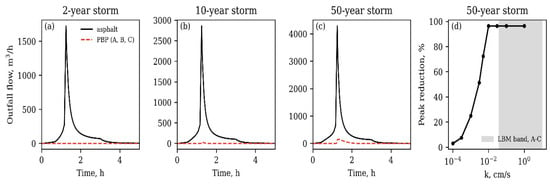
Figure 6. Runoff hydrographs for asphalt pavement and PBP for storm events with return periods of 2 (a), 10 (b), and 50 years (c); reduction in peak discharge as a function of the filtration coefficient for a 50-year storm (d); the range of k estimates for compositions A–C is shown in gray.

Compositions A, B, and C yield identical results for the central estimate of the filtration coefficient and at the lower limit of its uncertainty interval (±1.96 standard deviation). The permeability of all three mixtures (at least 0.04 cm/s, or 1400 mm/h) is many times greater than twice the peak intensity of a 50-year storm (375 mm/h), while the pore capacity of the pavement and subgrade (108–125 mm) exceeds the water layer reaching the pavement (up to 88 mm). Residual runoff during 10- and 50-year downpours occurs in water-permeable areas of the watershed where precipitation intensity exceeds the rate of infiltration into the soil.

The effect of permeability is evident only when k < 0.01 cm/s: at k = 0.005 cm/s, the reduction in peak discharge decreases to 72%, and at k = 0.001 cm/s, to 25% (Figure 6d). This threshold is 4–19 times lower than the lower limit of the k estimate for the compositions in Table 3. The uncertainty of the filtration coefficient, established in Section 2.1.2, does not affect the hydrological result. The permeability margin determines the permissible degree of clogging: a several-fold decrease in k during operation will not alter the pavement’s performance under the assumed storm events.

4. Discussion

4.1. Strength: What the Model Explains and What Remains Beyond Its Scope

The strength of permeable concrete in the collected data is determined primarily by porosity. The mean absolute SHAP value for porosity is 4.90 MPa; for the remaining four variables, it ranges from 0.09 to 0.24 MPa (the contribution of microsilica is not estimated based on these data; see Section 3.2). The break in the dependence of the porosity contribution at P_c ≈ 24% indicates that strength decreases more sharply above this value. Apparently, above this threshold, the number of contacts between grains bound by cement paste decreases faster than the volume of voids increases.

The variation in strength for the same composition is large and is associated with differences between laboratories that are not reflected in the input variables. The most illustrative study involved compacting the same mixture using vibration for durations ranging from 0 to 60 s [44]. In this case, the strength increased from 12.8 to 28.4 MPa, while the porosity decreased from 20.7 to 7.0%. The type and size of the specimen (cube or cylinder), the compaction method, and the type of aggregate (natural crushed stone, recycled concrete, steelmaking slag, ash–slag aggregate) vary from study to study. Therefore, when transferring the model to a new study, the average absolute error is approximately 5 MPa, and R² does not exceed 0.45 for any model when studies are sequentially excluded.

Including physical terms in the loss function improves the accuracy of the transfer, but the improvement does not exceed the confidence interval. Without these terms, the model explains 43% of the strength variance in the test studies; with them, it explains 74%. However, when studies are excluded one at a time, linear regression (R² = 0.45) outperforms PIML (0.31). With 28 data sources, increasing the model’s complexity does not yield any advantage over a simple relationship in which porosity plays the primary role. The “strength–porosity” relationship, defined by Equation (1), provides the network with the correct general trend of the relationship but does not eliminate interlaboratory variation.

In the presence of noise in the input data, PIML retains an advantage over the network without physical terms (R² 0.35–0.39 versus 0.34), although the difference decreases as noise increases. Outside the range of physically incorrect data, none of the networks produced incorrect predictions; therefore, for this dataset, physical constraints improve the accuracy of the transfer but are not a prerequisite for the plausibility of the predictions.

4.2. Why the Filtration Coefficient Cannot Be Predicted

None of the tested models predicted the filtration coefficient for the new studies better than their average value. The main reason appears to lie in the measurement methods rather than in a lack of composition variables. Test method. The median k value for variable head in the collected data is 0.84 cm/s, and for constant head, it is 0.38 cm/s.

Determination of porosity. For concrete made with ash–slag aggregate [29], with a total porosity of 19–37%, the filtration coefficient ranges from 0.006 to 0.56 cm/s, whereas in other studies, for the same porosity, its median is 1.04 cm/s (interquartile range 0.46–1.68 cm/s). Apparently, the total porosity of this concrete includes pores within the aggregate grains that do not contribute to filtration.

Until the method for measuring k is standardized, a model trained on a compilation of the literature data will reproduce the differences in methods rather than the material properties.

The LBM calculation provides a different basis for estimating k. It overestimates permeability by a factor of 50, but this discrepancy remains constant within the porosity range of 20–32.5% (p = 0.51 for the trend). The shape of the k(P_c) relationship is accurately reproduced, and the magnitude is brought into agreement with the experimental values by a single multiplier. The uncertainty band (±1.96 standard deviation) around the corrected curve (from 1/7 to 7 times the central value) reflects the spread of the experimental data. It is this band, rather than a point estimate, that is used in the hydrological calculation.

4.3. Pareto-Optimal Mix Designs and Hydrological Effect

The trade-off between strength, porosity, and carbon footprint is primarily resolved by selecting the porosity and cement content. Mixes A and B lie at the boundaries of the acceptable range: A at the lower porosity limit (15%), and B at the strength limit (10 MPa). There is no internal optimum within the training data. Cement consumption ranging from 336 kg/m³ (formulation C) to 431 kg/m³ (formulation A) determines the difference in the carbon footprint (311–397 kg CO₂-eq/m³); the emissions from microsilica and aggregate account for no more than 3% of the carbon footprint, but microsilica reduces it by 4–9% by replacing a portion of the cement.

The effectiveness of the coating is determined by its area, its ratio to the area from which runoff flows onto it, the pore volume of the base, and the permeability of the underlying soil. The concrete mix design determines the bearing capacity and carbon footprint, and more than adequately ensures the hydraulic function under such conditions.

This determines the design procedure. Porosity is selected based on the required strength using a model. Then, the condition k ≥ 0.01 cm/s is verified, taking into account expected clogging. The thickness and porosity of the base are determined based on the design storm. A permeability margin of 4–19 times determines the permissible decrease in k during operation: as long as it does not exceed this margin, clogging does not affect the pavement’s performance under the assumed rainfall events. It is possible to incorporate the strength model and the k(P_c) relationship into design decision-support tools, including digital models of urban infrastructure [51]. No software implementation of such a tool was carried out in this study.

4.4. Limitations of the Study

Data. The dataset includes 337 mixtures from 28 studies, comprising only values from tables and text. Studies presenting results solely in graphs (37 out of 108 excluded) were not used. For 78 observations, the aggregate content or size was replaced with the median of the training sample. The model was trained on mixtures with porosity ranging from 6.3% to 36.5%. Optimization was restricted to the 5th–95th percentiles of the training data (W/C 0.22–0.35, aggregate content 71.8–81.9%, microsilica up to 8.3%) and porosity 15–29.5%; the aggregate size was assumed to be constant (9.5 mm). Microsilica was present in 72 of 236 training observations (7 studies) and in none of the test observations; the effect of the additive on the strength of the optimal mixtures was not verified using independent data.

Interlaboratory differences. The compaction method, sample type, and aggregate type are not included in the model; therefore, the error in transferring results to a new study (MAE approximately 5 MPa) is significantly higher than the error within a single study. The test sample consisting of four studies is small, and the estimate based on it (R² = 0.74) is higher than the estimate obtained by excluding one study at a time (R² = 0.31). Both estimates should be considered together. The model’s robustness to noise in the input data (Figure 3) was assessed using a single noise realization for each level; therefore, the variation in R² across realizations is undefined. The compositions in Table 3 were obtained by optimization using this model; therefore, their strengths (22.1, 15.8, and 10.0 MPa) are expected values with errors of the same order of magnitude. Composition B lies on the constraint f_c ≥ 10 MPa, and its actual strength may turn out to be lower than required.

Sources. The selection is limited to open-access publications: 27 of the 28 included studies were published in MDPI journals, which may bias the sample in terms of methodologies and regions.

Carbon footprint. Stages A1–A3 were accounted for using fixed emission factors, excluding transportation, chemical additives, and variations in cement composition. When emission factors are varied (cement 0.90–0.91, aggregate 0.005–0.01, microsilica 0.014–0.10 kg CO₂-eq/kg), the carbon footprint of the mixtures changes by no more than 4%, and the order of the mixtures remains the same.

Interpretation. The SHAP values were calculated for 101 observations from the validation and test sets and characterize the model, not the hardening mechanism.

Filtration coefficient. It is estimated by calculating LBM on simplified microstructures: spherical grains, a cement paste shell of constant relative thickness, and an aggregate content of 0.31–0.42, which is lower than in actual concrete. The uncertainty range covers the experimental variation but does not replace the measurement of k for a specific mix design.

Hydrological calculation. Design storm events were derived using a standard formula with parameters typical of a temperate continental climate, without reference to a specific city. There is a single catchment area; the underlying soil has a permeability of 5 mm/h, and there is no drainage. Clogging and freezing of the foundation were not modeled. On low-permeability soils, with a higher area ratio, or during more intense downpours, the capacity of the foundation may become a limiting factor.

Durability. Frost resistance and changes in properties over time were not evaluated [65].

Experimental Verification. All quantitative results were obtained through calculation and require experimental verification. The strength predictions for the mixtures in Table 3 should be verified using specimens prepared according to a standardized method. The filtration coefficient of these same specimens should be measured under constant and variable head with the side surfaces sealed.

5. Conclusions

Of the 136 studies evaluated based on their full text, 28 open-access studies (337 mixtures) were selected according to the PRISMA guidelines. For each mixture, these studies specified the water–cement ratio, aggregate consumption or aggregate size, measured porosity, 28-day strength, and filtration coefficient.

The 28-day strength of permeable concrete is determined primarily by porosity: its contribution to the prediction (4.9 MPa) is an order of magnitude greater than the combined contribution of the W/C ratio, aggregate proportions, and aggregate size; based on available data, the effect of microsilica has not been established. The decline in strength accelerates when porosity exceeds 24%.

Incorporating the relationship between strength and porosity into the neural network’s loss function, along with the conditions for its monotonically decreasing behavior and physical boundaries, increased R² in the test studies from 0.43 to 0.74. The difference is not statistically significant. When studies were sequentially excluded, R² was 0.31 and was inferior to linear regression (0.45). Interlaboratory differences in compaction, sample type, and aggregates limit the accuracy of any model based on the literature data.

None of the tested models can be applied to new studies to determine the filtration coefficient, due to differences in the methods used to measure it and to determine porosity. Calculating the LBM for 500 virtual samples yields the form of the relationship k(P_c) without a systematic bias trend (p = 0.51), and after scaling to the experimental level by a constant factor β = 0.020, it provides an estimate of k with an uncertainty interval (±1.96 standard deviation).

Multiobjective optimization within the model’s applicability domain yielded three compositions:

A:

22.1 MPa, porosity 15%, 397 kg CO₂-eq/m³;

B:

10.0 MPa, porosity 26.5%, 343 kg CO₂-eq/m³;

C:

15.8 MPa, porosity 19.7%, 311 kg CO₂-eq/m³.

The difference in carbon footprint is determined by cement consumption.

In a hydrological model of a 5-hectare watershed, a permeable surface covering 1.5 hectares—which also receives runoff from an additional 1.5 hectares of impervious surfaces—reduces peak discharge by 96–100% during storm events with a recurrence interval of 2–50 years. Mixes A, B, and C yield identical results. Permeability limits the pavement’s performance only when k < 0.01 cm/s, which is 4–19 times lower than the estimates for the mixtures obtained. The concrete mix design should be selected based on strength requirements and carbon footprint, while hydraulic efficiency should be ensured by the pavement area and the base’s storage capacity.

The results were obtained through calculation. The next stage involves the production and testing of the mixtures listed in Table 3 using a standardized methodology, including measurements of strength and filtration coefficient with the side surfaces of the specimens sealed, as well as field testing at a pilot site.

References

- Fu, D.; Zhang, C.; Hall, J.W.; Butler, D. Are sponge cities the solution to China’s growing urban flooding problems? WIREs Water 2023, 10, e1613. [Google Scholar] [CrossRef] [Scilit]
- Li, H.; Harvey, J.T.; Holland, T.J.; Kayhanian, M. The use of reflective and permeable pavements as a potential practice for heat island mitigation and stormwater management. Environ. Res. Lett. 2013, 8, 015023, Corrigendum in Environ. Res. Lett. 2013, 8, 049501. https://doi.org/10.1088/1748-9326/8/4/049501. [Google Scholar] [CrossRef] [Scilit]
- Wang, J.; Meng, Q.; Zou, Y.; Qi, Q.; Tan, K.; Santamouris, M.; He, B.-J. Performance synergism of pervious pavement on stormwater management and urban heat island mitigation: A review of its benefits, key parameters, and co-benefits approach. Water Res. 2022, 221, 118755. [Google Scholar] [CrossRef] [Scilit] [PubMed]
- Bhat, A.H.; Sharma, S.K. Pervious concrete pavements: A comprehensive review of materials, performance, and sustainability. Innov. Infrastruct. Solut. 2025, 10, 326. [Google Scholar] [CrossRef] [Scilit]
- Lu, F.; Yang, L.; Jiang, Y. Optimum mix design and correlation analysis of pervious concrete. Materials 2025, 18, 4129. [Google Scholar] [CrossRef] [Scilit] [PubMed]
- Wu, Y.; Pieralisi, R.; Sandoval, F.G.B.; López Carreño, R.D.; Pujadas, P. Optimizing pervious concrete with machine learning: Predicting permeability and compressive strength using artificial neural networks. Constr. Build. Mater. 2024, 443, 137619. [Google Scholar] [CrossRef] [Scilit]
- Feng, D.-C.; Liu, Z.-T.; Wang, X.-D.; Chen, Y.; Chang, J.-Q.; Wei, D.-F.; Jiang, Z.-M. Machine learning-based compressive strength prediction for concrete: An adaptive boosting approach. Constr. Build. Mater. 2020, 230, 117000. [Google Scholar] [CrossRef] [Scilit]
- Yu, F.; Chu, W.; Zhang, R.; Gao, Z.; Yang, Y. Predicting the permeability and compressive strength of pervious concrete using a stacking ensemble machine learning approach. Sci. Rep. 2025, 15, 22506. [Google Scholar] [CrossRef] [Scilit] [PubMed]
- Zhang, J.; Huang, Y.; Ma, G.; Sun, J.; Nener, B. A metaheuristic-optimized multi-output model for predicting multiple properties of pervious concrete. Constr. Build. Mater. 2020, 249, 118803. [Google Scholar] [CrossRef] [Scilit]
- Karniadakis, G.E.; Kevrekidis, I.G.; Lu, L.; Perdikaris, P.; Wang, S.; Yang, L. Physics-informed machine learning. Nat. Rev. Phys. 2021, 3, 422–440. [Google Scholar] [CrossRef] [Scilit]
- Vadyala, S.R.; Betgeri, S.N.; Matthews, J.C.; Matthew, E. A review of physics-based machine learning in civil engineering. Results Eng. 2022, 13, 100316. [Google Scholar] [CrossRef] [Scilit]
- Rahman, M.A.; Zhang, T.; Lu, Y. PINN-CHK: Physics-informed neural network for high-fidelity prediction of early-age cement hydration kinetics. Neural Comput. Appl. 2024, 36, 13665–13687. [Google Scholar] [CrossRef] [Scilit]
- Rahman, M.A.; Lu, Y. EcoBlendNet: A physics-informed neural network for optimizing supplementary material replacement to reduce the carbon footprint during cement hydration. J. Clean. Prod. 2024, 464, 142777. [Google Scholar] [CrossRef] [Scilit]
- Chen, H.; Deng, T.; Du, T.; Chen, B.; Skibniewski, M.J.; Zhang, L. An RF and LSSVM–NSGA-II method for the multi-objective optimization of high-performance concrete durability. Cem. Concr. Compos. 2022, 129, 104446. [Google Scholar] [CrossRef] [Scilit]
- Li, J.; Xu, Z.; Hu, D. Deep Learning-Based Multiobjective Optimization Framework for Stormwater Management Models. J. Hydrol. Eng. 2026, 31. [Google Scholar] [CrossRef] [Scilit]
- Page, M.J.; McKenzie, J.E.; Bossuyt, P.M.; Boutron, I.; Hoffmann, T.C.; Mulrow, C.D.; Shamseer, L.; Tetzlaff, J.M.; Akl, E.A.; Brennan, S.E.; et al. The PRISMA 2020 statement: An updated guideline for reporting systematic reviews. BMJ 2021, 372, n71. [Google Scholar] [CrossRef] [Scilit]
- Hung, V.V.; Seo, S.-Y.; Kim, H.-W.; Lee, G.-C. Permeability and strength of pervious concrete according to aggregate size and blocking material. Sustainability 2021, 13, 426. [Google Scholar] [CrossRef] [Scilit]
- Adresi, M.; Yamani, A.; Tabarestani, M.K.; Nalon, G.H. A prediction model for the unconfined compressive strength of pervious concrete based on mix design and compaction energy variables using the response surface methodology. Buildings 2024, 14, 2834. [Google Scholar] [CrossRef] [Scilit]
- Liu, J.; Bakri, Z.; Li, F.; Jaffar, S.T.A. Strength–permeability optimization of FA–MK–NS blended pervious concrete based on response surface methodology. Buildings 2026, 16, 3335. [Google Scholar] [CrossRef] [Scilit]
- Zhan, Q.; Yin, C. A novel pervious concrete improved by hexagonal boron nitride and basalt fiber in mechanical properties, permeability, and micro-mechanisms. Buildings 2024, 14, 778. [Google Scholar] [CrossRef] [Scilit]
- Lee, M.-G.; Wang, Y.-C.; Wang, W.-C.; Hsieh, Y.-C. Abrasion and maintenance of high-strength fiber-reinforced pervious concrete. Buildings 2024, 14, 127. [Google Scholar] [CrossRef] [Scilit]
- Yuan, W.; Ji, L.; Meng, L.; Fang, M.; Zhang, X. Influence of mineral admixtures on the performance of pervious concrete and microscopic research. Buildings 2024, 14, 533. [Google Scholar] [CrossRef] [Scilit]
- Liu, H.; Luo, G.; Wang, L.; Gong, Y. Strength time–varying and freeze–thaw durability of sustainable pervious concrete pavement material containing waste fly ash. Sustainability 2019, 11, 176. [Google Scholar] [CrossRef] [Scilit]
- Liu, H.; Luo, G.; Wei, H.; Yu, H. Strength, permeability, and freeze-thaw durability of pervious concrete with different aggregate sizes, porosities, and water-binder ratios. Appl. Sci. 2018, 8, 1217. [Google Scholar] [CrossRef] [Scilit]
- Liu, F.; Li, Z.; Liu, B.; Yu, Z.; Li, Z.; Zhu, M.; Wang, Y.; Ding, X. Experimental and numerical investigations on the influences of target porosity and w/c ratio on strength and permeability of pervious concrete. Materials 2025, 18, 3951. [Google Scholar] [CrossRef] [Scilit] [PubMed]
- Chen, C.; Zhang, K.; Yin, Z.; Zhou, J. Deterioration performance of recycled aggregate pervious concrete under freezing–thawing cycle and chloride environment. Buildings 2023, 13, 645. [Google Scholar] [CrossRef] [Scilit]
- Peng, H.; Yin, J.; Song, W. Mechanical and hydraulic behaviors of eco-friendly pervious concrete incorporating fly ash and blast furnace slag. Appl. Sci. 2018, 8, 859. [Google Scholar] [CrossRef] [Scilit]
- Tamimi, A.; Tabsh, S.W.; El-Emam, M. Pervious concrete made with recycled coarse aggregate and reinforced with date palm leaves fibers. Materials 2023, 16, 7496. [Google Scholar] [CrossRef] [Scilit] [PubMed]
- Park, J.-H.; Jeong, S.-T.; Bui, Q.-T.; Yang, I.-H. Strength and permeability properties of pervious concrete containing coal bottom ash aggregates. Materials 2022, 15, 7847. [Google Scholar] [CrossRef] [Scilit] [PubMed]
- Mitrosz, O.; Kurpińska, M.; Miśkiewicz, M.; Brzozowski, T.; Abdelgader, H.S. Influence of the addition of recycled aggregates and polymer fibers on the properties of pervious concrete. Materials 2023, 16, 5222. [Google Scholar] [CrossRef] [Scilit] [PubMed]
- Yan, X.; Wang, X.; Sun, C.; Xin, M.; He, J. Performance analysis and admixture optimization of GBFS-HPMC/fiber pervious concrete. Materials 2023, 16, 6455. [Google Scholar] [CrossRef] [Scilit] [PubMed]
- Zhu, H.; Wen, C.; Wang, Z.; Li, L. Study on the permeability of recycled aggregate pervious concrete with fibers. Materials 2020, 13, 321. [Google Scholar] [CrossRef] [Scilit] [PubMed]
- Wu, R.; Shi, S.; Shen, Y.; Hu, C.; Luo, M.; Gan, Z.; Xiao, B.; Wang, Z. Effects of different factors on the performance of recycled aggregate permeable pavement concrete. Materials 2022, 15, 4566. [Google Scholar] [CrossRef] [Scilit] [PubMed]
- Bao, X.; Liao, W.; Dong, Z.; Wang, S.; Tang, W. Development of vegetation-pervious concrete in grid beam system for soil slope protection. Materials 2017, 10, 96. [Google Scholar] [CrossRef] [Scilit] [PubMed]
- Barišić, I.; Netinger Grubeša, I.; Dokšanović, T.; Zvonarić, M. Influence of clogging and unbound base layer properties on pervious concrete drainage characteristics. Materials 2020, 13, 2455. [Google Scholar] [CrossRef] [Scilit] [PubMed]
- Jiao, W.; Peng, Z.; Ma, B.; Dai, C.; Gong, B.; Huang, Z. Performance testing and evaluation of double-layer pervious concrete based on recycled aggregates. Materials 2026, 19, 1067. [Google Scholar] [CrossRef] [Scilit] [PubMed]
- Liu, H.; Luo, G.; Wang, L.; Wang, W.; Li, W.; Gong, Y. Laboratory evaluation of eco-friendly pervious concrete pavement material containing silica fume. Appl. Sci. 2019, 9, 73. [Google Scholar] [CrossRef] [Scilit]
- Xie, H.Z.; Li, L.G.; Liu, F.; Kwan, A.K.H. Recycling old concrete as waste concrete powder for use in pervious concrete: Effects on permeability, strength and eco-friendliness. Buildings 2022, 12, 2172. [Google Scholar] [CrossRef] [Scilit]
- Gratão, U.; Innocentini, M.D.M.; Simão, L. Processing parameters for pervious concrete with basalt and CDW aggregates: Addressing the strength–porosity–permeability trade-off. Waste 2026, 4, 25. [Google Scholar] [CrossRef] [Scilit]
- Alex, A.G.; Jose, P.A.; Saberian, M.; Li, J. Green pervious concrete containing diatomaceous earth as supplementary cementitious materials for pavement applications. Materials 2023, 16, 48. [Google Scholar] [CrossRef] [Scilit] [PubMed]
- Fu, J.; Jiang, L.; Yang, M.; Yu, D.; Shen, M.; Wang, Y. Influence of nano-silica and porosity on the strength and permeability of permeable concrete: An experimental study. Buildings 2026, 16, 148. [Google Scholar] [CrossRef] [Scilit]
- Tang, C.-W.; Cheng, C.-K.; Tsai, C.-Y. Mix design and mechanical properties of high-performance pervious concrete. Materials 2019, 12, 2577. [Google Scholar] [CrossRef] [Scilit] [PubMed]
- Paula Junior, A.; Jacinto, C.; Oliveira, T.; Polisseni, A.; Brum, F.; Teixeira, E.; Mateus, R. Characterisation and life cycle assessment of pervious concrete with recycled concrete aggregates. Crystals 2021, 11, 209. [Google Scholar] [CrossRef] [Scilit]
- Mitrosz, O.; Kurpińska, M.; Miśkiewicz, M.; Brzozowski, T. Effect of vibration duration on strength and permeability of pervious concrete with recycled aggregate and low-carbon cements. Sci. Rep. 2025, 15, 35905. [Google Scholar] [CrossRef] [Scilit] [PubMed]
- Sukop, M.C.; Thorne, D.T. Lattice Boltzmann Modeling: An Introduction for Geoscientists and Engineers; Springer: Berlin/Heidelberg, Germany, 2006. [Google Scholar] [CrossRef]
- Torquato, S.; Uche, O.U.; Stillinger, F.H. Random sequential addition of hard spheres in high Euclidean dimensions. Phys. Rev. E 2006, 74, 061308. [Google Scholar] [CrossRef] [Scilit] [PubMed]
- Neithalath, N.; Bentz, D.P.; Sumanasooriya, M.S. Predicting the permeability of pervious concrete. ACI Concr. Int. 2010, 32, 35–40. [Google Scholar]
- Narváez, A.; Zauner, T.; Raischel, F.; Hilfer, R.; Harting, J. Quantitative analysis of numerical estimates for the permeability of porous media from lattice-Boltzmann simulations. J. Stat. Mech. Theory Exp. 2010, 2010, P11026. [Google Scholar] [CrossRef] [Scilit]
- Zhao, D.; Xu, J.; Wang, X.; Guo, Q.; Li, Y.; Han, Z.; Liu, Y.; Zhang, Z.; Zhang, J.; Sun, R. Numerical study on permeability of reconstructed porous concrete based on lattice Boltzmann method. Buildings 2024, 14, 1182. [Google Scholar] [CrossRef] [Scilit]
- Krüger, T.; Kusumaatmadja, H.; Kuzmin, A.; Shardt, O.; Silva, G.; Viggen, E.M. The Lattice Boltzmann Method: Principles and Practice; Springer: Berlin/Heidelberg, Germany, 2017. [Google Scholar] [CrossRef] [Scilit]
- Lei, B.; Janssen, P.; Stoter, J.; Biljecki, F. Challenges of urban digital twins: A systematic review and a Delphi expert survey. Autom. Constr. 2023, 147, 104716. [Google Scholar] [CrossRef] [Scilit]
- Pan, C.; Luo, L.-S.; Miller, C.T. An evaluation of lattice Boltzmann schemes for porous medium flow simulation. Comput. Fluids 2006, 35, 898–909. [Google Scholar] [CrossRef] [Scilit]
- Zou, Q.; He, X. On pressure and velocity boundary conditions for the lattice Boltzmann BGK model. Phys. Fluids 1997, 9, 1591–1598. [Google Scholar] [CrossRef] [Scilit]
- Kingma, D.P.; Ba, J. Adam: A method for stochastic optimization. In Proceedings of the 3rd International Conference on Learning Representations (ICLR 2015), San Diego, CA, USA, 7–9 May 2015. [Google Scholar]
- Lundberg, S.M.; Lee, S.-I. A unified approach to interpreting model predictions. Adv. Neural Inf. Process. Syst. 2017, 30, 4765–4774. [Google Scholar]
- Štrumbelj, E.; Kononenko, I. Explaining prediction models and individual predictions with feature contributions. Knowl. Inf. Syst. 2014, 41, 647–665. [Google Scholar] [CrossRef] [Scilit]
- Antunes, L.N.; Ghisi, E.; Thives, L.P. Permeable Pavements Life Cycle Assessment: A Literature Review. Water 2018, 10, 1575. [Google Scholar] [CrossRef] [Scilit]
- Jones, C.; Hammond, G. Inventory of Carbon and Energy (ICE) Database; Version 3.0; Circular Ecology: Bristol, UK, 2019; Available online: https://circularecology.com/embodied-carbon-footprint-database.html (accessed on 10 October 2026).
- Kevern, J. 522R-10: Report on Pervious Concrete; American Concrete Institute: Farmington Hills, MI, USA, 2010; 38p. [Google Scholar]
- Deb, K.; Pratap, A.; Agarwal, S.; Meyarivan, T. A fast and elitist multiobjective genetic algorithm: NSGA-II. IEEE Trans. Evol. Comput. 2002, 6, 182–197. [Google Scholar] [CrossRef] [Scilit]
- Rossman, L.A.; Simon, M.A. Storm Water Management Model User’s Manual, Version 5.2; EPA/600/R-22/030; U.S. Environmental Protection Agency: Washington, DC, USA, 2022. Available online: https://www.epa.gov/system/files/documents/2022-04/swmm-users-manual-version-5.2.pdf (accessed on 10 October 2026).
- Platz, M.; Simon, M.; Tryby, M. Testing of the Storm Water Management Model Low Impact Development Modules. J. Am. Water Resour. Assoc. 2020, 56, 283–296. [Google Scholar] [CrossRef] [Scilit] [PubMed]
- SN RK 4.01-03-2011; Wastewater Disposal. External Networks and Structures (as Amended as of December 29, 2021). Agency of the Republic of Kazakhstan for Construction and Housing and Communal Services: Astana, Kazakhstan, 2011. Available online: https://prg.kz/document/?doc_id=31130718 (accessed on 10 October 2026).
- Chow, V.T.; Maidment, D.R.; Mays, L.W. Applied Hydrology; McGraw-Hill: Columbus, OH, USA, 1988; 572p. [Google Scholar]
- Henderson, V.; Tighe, S. Evaluation of pervious concrete pavement performance in cold weather climates. Int. J. Pavement Eng. 2012, 13, 197–208. [Google Scholar] [CrossRef] [Scilit]
Disclaimer/Publisher’s Note: The statements, opinions and data contained in all publications are solely those of the individual author(s) and contributor(s) and not of MDPI and/or the editor(s). MDPI and/or the editor(s) disclaim responsibility for any injury to people or property resulting from any ideas, methods, instructions or products referred to in the content. |
© 2026 by the authors. Licensee MDPI, Basel, Switzerland. This article is an open access article distributed under the terms and conditions of the Creative Commons Attribution (CC BY) license.