Offline-Certified Robust Block Backstepping for Perturbed Underactuated Mechanical Systems

Abstract

This paper develops certifiable enhancements to a block-backstepping controller for n-DOF underactuated mechanical systems in the Spong normal form. Two offline-computable tests, each reducible to a finite algebraic computation over a prescribed compact domain, are established: a minimum singular-value margin certifying uniform invertibility of the decoupling matrix, and a Jacobian Hurwitz condition certifying local exponential stability of the zero dynamics—the latter derived via an implicit zero-manifold parametrisation. Robustness overlays are introduced, comprising a bi-power term on the velocity-error channel and a matched-disturbance observer. Together, they supply an explicit observer transient budget and a practical entrance bound $t_o\left(\epsilon \right)+T_{\mathrm{ent}}$ for $\parallel {\dot{z}}_1{\parallel }_2$. No finite-time convergence of the complete closed-loop state is claimed. The resulting workflow permits offline tuning and verification prior to deployment. A simulation on a high-fidelity cart–pendulum model is consistent with those bounds; it is not a substitute for the offline certificates.

1. Introduction and Problem Formulation

Underactuated mechanical systems arise across a broad range of engineering platforms, including cable-suspended aerial manipulators, variable-stiffness series-elastic robots, ship fin stabilisers, and spacecraft with reaction-wheel attitude control—anywhere the number of independent actuators is fewer than the degrees of freedom to be regulated [1,2,3,4,5]. The breadth of this system class has been systematically catalogued in several survey treatments [6,7,8]. Although partial feedback linearisation emerged as a standard approach in Spong’s framework [2], the inherent actuation deficit impedes system representation in the standard normal form [9,10,11]. Consequently, this precludes the straightforward application of integral backstepping; however, appropriate coordinate transformations can decompose the dynamics into a cascaded structure [12,13], thereby enabling the use of block backstepping [14]. Block backstepping for underactuated systems [15,16] proceeds by constructing a diffeomorphism that decomposes the closed-loop into a cascade and a zero-dynamics subsystem, then stabilising each independently. This structural decomposition provides a constructive, Lyapunov-based framework [17,18] that systematically circumvents the restrictive matching conditions of standard feedback linearisation [19]. An alternative means of avoiding the recursive differentiation intrinsic to standard backstepping is afforded by command-filtered variants [20,21], subsequently extended to adaptive and disturbance-attenuating formulations [22,23,24]; these approaches, however, address analytic tractability rather than the structural actuation deficit that motivates the cascaded block-backstepping decomposition adopted herein. Data-driven alternatives have likewise been investigated for this problem class [25,26], typically at the expense of the a priori stability certificates that the present Lyapunov-based construction is designed to retain.

The nominal block backstepping architecture [15] forms the baseline for an n-DOF underactuated system with $n_2$ actuated degrees of freedom ($n_2<n$). Defining the column concatenation operator $\mathrm{col}(v_1,\dots ,v_k){\left[\begin{array}{ccc}{v}_1^{\top }& \dots & v_k^{\top }\end{array}\right]}^{\top },$ the configuration is partitioned into unactuated degrees of freedom $q_1\in {\mathbb{R}}^{n_1}$ and actuated degrees of freedom $q_2\in {\mathbb{R}}^{n_2}$, with $n_1+n_2=n$. Whilst velocities are denoted $p_i:={\dot{q}}_i$, the full state vector is defined as $X:=\mathrm{col}(q_1,p_1,q_2,p_2)\in {\mathbb{R}}^{2n}$. Following Spong’s partial feedback linearisation ([9], Equation (4)), the plant dynamics are given by

$$\begin{array}{c}\hfill \begin{array}{cc}\hfill {\dot{q}}_1& =p_1,\hfill \\ \hfill {\dot{q}}_2& =p_2,\hfill \\ \hfill {\dot{p}}_1& =f(q,p)+g\left(q\right)\left(u+d\left(t\right)\right),\hfill \\ \hfill {\dot{p}}_2& =u+d\left(t\right),\hfill \end{array}\end{array}$$

(1)

where $d\left(t\right):{\mathbb{R}}_{\ge 0}\to {\mathbb{R}}^{n_2}$ denotes a bounded disturbance. Define ${\mathrm{\Omega }}_q\subset {\mathbb{R}}^n$ as the compact set of mechanically permissible configurations, and let $\overline{p}>0$ be a strict velocity bound derived from physical actuation limits. The compact state-space operating domain is defined as

$${\mathrm{\Omega }}_X\left\{X\in {\mathbb{R}}^{2n}\mid q=\mathrm{col}(q_1,q_2)\in {\mathrm{\Omega }}_q,{\parallel p\parallel }_{\infty }\le \overline{p}\right\},$$

and is chosen so that $0\in \mathrm{int}{\mathrm{\Omega }}_X$. To ensure that the nominal control law is well-defined and continuous on ${\mathrm{\Omega }}_X$, the minimal construction regularity $f\in C^1({\mathrm{\Omega }}_X,{\mathbb{R}}^{n_1})$ and $g\in C^2({\mathrm{\Omega }}_q,{\mathbb{R}}^{n_1\times n_2})$ is imposed [27].

Introducing a constant matrix $K\in {\mathbb{R}}^{n_2\times n_1}$, the first error coordinate is defined as

$$z_1:=q_2-K\left(q_1+p_1-g\left(q\right)p_2\right)$$

with the integral state ${\chi }_1:={\int }_0^t{z}_1\left(\tau \right)d\tau$, which is augmented to eliminate the steady-state offset in $z_1$. Denoting the time derivative $\dot{g}(q,p):={\sum }_{i=1}^n{\displaystyle \frac{\partial g}{\partial q_i}}{p}_i$, the virtual control [15] for the unperturbed plant (i.e., $d\left(t\right)\equiv 0;$ henceforth, the unperturbed plant is referred to as the nominal plant) is formulated as

$${\alpha }_1(X,{\chi }_1):=-c_1{z}_1-\lambda {\chi }_1+K\left(p_1+f(q,p)-\dot{g}(q,p)p_2\right)$$

for constants $c_1,\lambda >0$, which yields the second error coordinate $z_2:=p_2-{\alpha }_1(X,{\chi }_1)$. Consequently, the $z_1$-channel dynamics become

$${\dot{z}}_1=-c_1{z}_1-\lambda {\chi }_1+z_2.$$

Differentiating $z_2$ along the nominal trajectories yields

$${\dot{z}}_2=c_1{z}_2-(c_1^2-\lambda )z_1-\lambda c_1{\chi }_1+\varphi \left(X\right)+\psi \left(X\right)u.$$

Omitting the detailed block-strict feedback derivation ([16], Chapter 3), the resulting nominal control inherently depends on the decoupling matrix $\psi :{\mathbb{R}}^{2n}\to {\mathbb{R}}^{n_2\times n_2}$ and the lumped nonlinearity $\varphi :{\mathbb{R}}^{2n}\to {\mathbb{R}}^{n_2}$. Define the matrices ${\ddot{g}}_o:=(q,p){\sum }_{i,j=1}^n{\displaystyle \frac{{\partial }^{2}g}{\partial q_j\partial q_i}}{p}_j{p}_i\in {\mathbb{R}}^{n_1\times n_2}$, ${\nabla }_1{\displaystyle \frac{\partial \left(g{p}_2\right)}{\partial q_1}}\in {\mathbb{R}}^{n_1\times n_1}$ and ${\nabla }_2{\displaystyle \frac{\partial \left(g{p}_2\right)}{\partial q_2}}\in {\mathbb{R}}^{n_1\times n_2}$. The definitions of $\psi \left(X\right)$ and $\varphi \left(X\right)$ are as follows:

$$\begin{array}{cc}\hfill \psi \left(X\right):=& I-K\left(g+\left({\partial }_{p_1}f\right)g+{\partial }_{p_2}f-\dot{g}-{\nabla }_{1}g-{\nabla }_2\right),\hfill \\ \hfill \varphi \left(X\right):=& -K\left(f+\left({\partial }_{q_1}f\right)p_1+\left({\partial }_{q_2}f\right)p_2+\left({\partial }_{p_1}f\right)f-{\ddot{g}}_o{p}_2-{\nabla }_{1}f\right).\hfill \end{array}$$

In the above description, ${\partial }_v(·)$ denotes the Jacobian matrix with respect to a generic vector v. The aforementioned standing regularity hypotheses ensure that $\varphi$ and $\psi$ are well-defined and continuous on ${\mathrm{\Omega }}_X$.

Enforcing the exponentially stable closed-loop cascade

$${\dot{z}}_2=-z_1-c_2{z}_2,$$

with $c_2>0$, yields the backstepping law for the nominal plant (i.e., (2) with $d\left(t\right)\equiv 0$):

$$u_{\mathrm{bb}}:=-\psi {\left(X\right)}^{-1}\left(C_1{z}_1+C_2{z}_2-\lambda c_1{\chi }_1+\varphi \left(X\right)\right)$$

(2)

where $C_1:=1-c_1^2+\lambda ,C_2:=c_1+c_2$.

Under the structural assumptions established in [15], this law exponentially stabilises the nominal cascade in $(z_1,z_2,{\chi }_1)$. However, it lacks a priori certification guaranteeing the uniform invertibility of $\psi \left(X\right)$ over a prescribed compact operating set, leaves the internal zero dynamics unverified, and fails to quantify robustness against persistent matched disturbances.

Building upon this framework, this work provides three key contributions that resolve the open issues identified previously:

• A singularity-margin certificate for the invertibility of $\psi \left(X\right)$ on ${\mathrm{\Omega }}_X$, computed offline with an explicit ${\parallel \psi \left(X\right)}^{-1}{\parallel }_2$ bound [28,29,30].
• An a priori Hurwitz condition on the zero-manifold Jacobian, derived via the implicit function theorem to certify local exponential stability [31,32].
• Composite robustness overlays comprising an Extended State Observer (ESO) [33,34,35,36,37] that yields the ultimate bound $\underset{t\to \infty }{\mathrm{lim\; sup}}{\parallel \tilde{d}\left(t\right)\parallel }_2\le 2{\overline{d}}_1/{\omega }_o$ and a complete transient budget $E_{\sup }$, and a bi-power term [38] that enforces the practical entrance time $t_o\left(\epsilon \right)+T_{\mathrm{ent}}$ for $\parallel {\dot{z}}_1{\parallel }_2$. No finite-time convergence of the complete state is asserted.

2. Offline Certificates

This section separates analytical sufficient conditions from their computational verification. In particular, the nonsingularity of the decoupling matrix and stability of the zero dynamics are properties to be tested, rather than properties imposed in the operating-domain assumptions. A successful verification supplies a certificate for the specified model and domain; an inconclusive computation does not establish either stability or instability.

2.1. Operating Domain and Transformation Time Scale

Assumption 1 (Domain and regularity).

The compact operating domain ${\mathrm{\Omega }}_X$ contains the origin in its interior. The functions f and g are defined on an open neighbourhood of the operating domain, with $f\in C^1$ and $g\in C^2$. In a neighbourhood of the equilibrium, $f\in C^2$ and $g\in C^3$. The nominal plant has an equilibrium at the origin, so that $f(0,0)=0$. No nonsingularity assumption on ψ is included here.

For the numerical implementation, introduce a time scale $T_b>0$ and use

$$\begin{array}{cc}\hfill z_1& =q_2-K\left(q_1+T_b{p}_1-T_{b}g\left(q\right)p_2\right),\hfill \end{array}$$

(3a)

$$\begin{array}{cc}\hfill {\dot{\chi }}_1& =z_1,\hfill \end{array}$$

(3b)

$$\begin{array}{cc}\hfill s_0\left(X\right)& =p_1+T_{b}f(q,p)-T_b\dot{g}(q,p)p_2,\hfill \end{array}$$

(3c)

$$\begin{array}{cc}\hfill {\alpha }_1& =-c_1{z}_1-\lambda {\chi }_1+K{s}_0\left(X\right),\hfill \end{array}$$

(3d)

$$\begin{array}{cc}\hfill z_2& =p_2-{\alpha }_1.\hfill \end{array}$$

(3e)

The transformation in Section 1 is recovered by setting $T_b=1$. All occurrences of $z_1$, $z_2$, ${\alpha }_1$, $\varphi$ and $\psi$ below refer to the same selected value of $T_b$.

The matched-disturbance structure in (1) gives the exact cancellation

$${\dot{z}}_1=p_2-K{s}_0\left(X\right)=-c_1{z}_1-\lambda {\chi }_1+z_2.$$

Using the derivative notation introduced in Section 1, define

$$\begin{array}{cc}\hfill \mathcal{A}\left(X\right)=& f+T_b\left(\left({\partial }_{q_1}f\right)p_1+\left({\partial }_{q_2}f\right)p_2+\left({\partial }_{p_1}f\right)f-{\ddot{g}}_o{p}_2-{\nabla }_{1}f\right),\hfill \end{array}$$

(4a)

$$\begin{array}{cc}\hfill \mathcal{B}\left(X\right)=& g+T_b\left(\left({\partial }_{p_1}f\right)g+{\partial }_{p_2}f-\dot{g}-{\nabla }_{1}g-{\nabla }_2\right),\hfill \end{array}$$

(4b)

$$\begin{array}{cc}\hfill \varphi \left(X\right)& =-K\mathcal{A}\left(X\right),\hfill \end{array}$$

(4c)

$$\begin{array}{cc}\hfill \psi \left(X\right)& =I-K\mathcal{B}\left(X\right).\hfill \end{array}$$

(4d)

Consequently,

$${\ddot{z}}_1=\varphi \left(X\right)+\psi \left(X\right)(u+d).$$

These identities are also used to check consistency between the analytical model and its numerical implementation.

2.2. Verified Decoupling-Matrix Bounds

Let ${\left\{B_j\right\}}_{j=1}^{N_B}$ be a finite collection of closed boxes covering ${\mathrm{\Omega }}_X$. On each box, construct an interval enclosure

$$\psi \left(B_j\right)\subseteq {\left[\mathrm{\Psi }\right]}_j=M_j+[-R_j,R_j],$$

where $R_j$ is componentwise nonnegative. The enclosure must include all state dependence and every uncertain parameter included in the claim. For a numerical certificate, elementary functions and matrix operations must be evaluated using verified outward rounding.

Suppose that verified bounds

$${\underline{s}}_j\le {\sigma }_{\min }\left(M_j\right),{\parallel R_j\parallel }_F\le {\overline{r}}_j$$

are available. Define

$${\underline{\sigma }}_j={\underline{s}}_j-{\overline{r}}_j,\underline{\sigma }=\underset{1\le j\le N_B}{\min }{\underline{\sigma }}_j.$$

An ordinary floating-point singular-value calculation without a verified error bound is not sufficient for evaluating ${\underline{s}}_j$.

Proposition 1 (Computable uniform decoupling certificate).

Under Assumption 1, if the verified box enclosures satisfy $\underline{\sigma }>0$, then $\psi \left(X\right)$ is nonsingular throughout ${\mathrm{\Omega }}_X$ and

$${\sigma }_{★}:=\underset{X\in {\mathrm{\Omega }}_X}{\min }{\sigma }_{\min }\left(\psi \left(X\right)\right)\ge \underline{\sigma }>0,{\parallel \psi {\left(X\right)}^{-1}\parallel }_2\le {\underline{\sigma }}^{-1}.$$

Proof. 

For $X\in B_j$, write $\psi \left(X\right)=M_j+E_j\left(X\right)$. Componentwise enclosure gives $\parallel E_j{\left(X\right)\parallel }_2\le {\parallel E_j\left(X\right)\parallel }_F\le {\overline{r}}_j$. The singular-value perturbation inequality yields

$${\sigma }_{\min }\left(\psi \left(X\right)\right)\ge {\sigma }_{\min }\left(M_j\right)-{\parallel E_j\left(X\right)\parallel }_2\ge {\underline{\sigma }}_j.$$

Taking the minimum over the covering boxes proves the result. □

For scalar decoupling functions, the calculation simplifies. If $\psi \left(B_j\right)\subseteq [{\underline{\psi }}_j,{\overline{\psi }}_j]$ and this interval does not contain zero, then

$${\underline{\sigma }}_j=\min \left\{\right|{\underline{\psi }}_j|,|{\overline{\psi }}_j\left|\right\}.$$

An upper bound needed in the robustness analysis is obtained from the same enclosures:

$$\overline{\psi }\ge \underset{X\in {\mathrm{\Omega }}_X}{\sup }{\parallel \psi \left(X\right)\parallel }_2.$$

The offline procedure is as follows:

1.

Specify the operating domain, parameter set and controller transformation;

2.

Construct verified interval enclosures on an initial box partition;

3.

Accept boxes having a strictly positive lower bound;

4.

Bisect unresolved boxes and repeat;

5.

Report either a positive global lower bound or an inconclusive result at the prescribed computational limit.

Dense sampling may be reported as a diagnostic, but is not used in place of the verified covering calculation. No claim is made that an arbitrary nonlinear verification problem necessarily terminates after a prescribed finite number of subdivisions.

2.3. Constructive Zero-Dynamics Test

Set

$$\eta =\mathrm{col}(q_1,p_1),\xi =\mathrm{col}(q_2,p_2),$$

and define

$$C_0(\eta ,\xi )=\mathrm{col}\left(z_1(\eta ,\xi ),z_2(\eta ,\xi ,0)\right).$$

At the equilibrium, calculate

$$J_{\eta }={\left.{\displaystyle \frac{\partial C_0}{\partial \eta }}\right|}_0,J_{\xi }={\left.{\displaystyle \frac{\partial C_0}{\partial \xi }}\right|}_0.$$

Assumption 2 (Successful local zero-manifold test).

The equilibrium satisfies $C_0(0,0)=0$. The explicitly constructed matrix $J_{\xi }$ is nonsingular, as established either analytically or by a verified positive lower bound

$${\sigma }_{\min }\left(J_{\xi }\right)\ge {\underline{\sigma }}_{\iota }>0.$$

By the implicit function theorem, the constraints locally define $\xi =\iota \left(\eta \right)$, where

$$\iota \left(0\right)=0,D\iota \left(0\right)=-J_{\xi }^{-1}{J}_{\eta }.$$

Define

$$u_0\left(X\right)=-\psi {\left(X\right)}^{-1}\varphi \left(X\right)$$

and

$$H(\eta ,\xi )=\mathrm{col}\left(p_1,f(q,p)+g\left(q\right)u_0\left(X\right)\right).$$

The zero-dynamics Jacobian is therefore constructed directly as

$$A_{\mathcal{Z}}=H_{\eta }\left(0\right)-H_{\xi }\left(0\right)J_{\xi }^{-1}{J}_{\eta }.$$

(5)

Thus, no explicit nonlinear solution for $\iota$ is required.

A numerical implementation shall report $J_{\xi }$, its nonsingularity measure, $A_{\mathcal{Z}}$ and the eigenvalues of $A_{\mathcal{Z}}$. For a verified floating-point Hurwitz test, one may construct $P_{\mathcal{Z}}=P_{\mathcal{Z}}^{\top }>0$ and verify

$$A_{\mathcal{Z}}^{\top }{P}_{\mathcal{Z}}+P_{\mathcal{Z}}{A}_{\mathcal{Z}}<0.$$

For a scalar second-order zero-dynamics model, exact coefficient Sign conditions may be used instead.

Lemma 1 (Invariant augmented zero manifold).

Suppose the decoupling and zero-manifold tests succeed. The local invariant augmented zero manifold is

$${\mathcal{M}}_0=\{(X,{\chi }_1):C_0(\eta ,\xi )=0,{\chi }_1=0\}.$$

On this manifold, $u_{\mathrm{bb}}=u_0$ and $\dot{\eta }=H(\eta ,\iota \left(\eta \right))$.

Proof. 

On $z_1=z_2=0$, the identity ${\dot{z}}_1=-\lambda {\chi }_1$ shows that invariance requires ${\chi }_1=0$. Conversely, under $u_0$, the three derivatives ${\dot{\chi }}_1$, ${\dot{z}}_1$ and ${\dot{z}}_2$ vanish on $z_1=z_2={\chi }_1=0$. The remaining dynamics are precisely the stated internal dynamics. □

2.4. Explicit Error-Subsystem Stability Test

Lemma 2 (Nominal error dynamics).

For $c_1,c_2,\lambda >0$, the nominal augmented error dynamics

$${\dot{z}}_{\chi }=(A_E\otimes I_{n_2})z_{\chi },z_{\chi }=\mathrm{col}({\chi }_1,z_1,z_2),$$

with

$$A_E=\left[\begin{array}{ccc}0& 1& 0\\ -\lambda & -c_1& 1\\ 0& -1& -c_2\end{array}\right],$$

are exponentially stable.

Proof. 

The characteristic polynomial of $A_E$ is

$$p_E\left(s\right)=s^3+(c_1+c_2)s^2+(c_1{c}_2+\lambda +1)s+\lambda c_2.$$

All coefficients are positive. The remaining cubic Routh–Hurwitz inequality is

$$(c_1+c_2)(c_1{c}_2+\lambda +1)>\lambda c_2.$$

Its left-hand side minus its right-hand side equals

$$c_1{c}_2(c_1+c_2)+\lambda c_1+c_1+c_2>0.$$

Hence, $A_E$ is Hurwitz. The Kronecker product repeats its eigenvalues $n_2$ times, establishing the result. □

Theorem 1 (Nominal local exponential stability).

Suppose the decoupling certificate and Assumption 2 hold, and the matrix $A_{\mathcal{Z}}$ constructed in (5) is Hurwitz. Then, the nominal augmented equilibrium $(X,{\chi }_1)=(0,0)$ is locally exponentially stable.

Proof. 

The map

$$\mathrm{\Theta }(X,{\chi }_1)=\mathrm{col}(\eta ,{\chi }_1,z_1,z_2)$$

has a nonsingular Jacobian at the origin because $J_{\xi }$ is nonsingular. In these local coordinates, the nominal closed-loop linearisation is block triangular, with diagonal blocks $A_{\mathcal{Z}}$ and $A_E\otimes I_{n_2}$. Both blocks are Hurwitz. The nominal vector field is $C^1$ near the equilibrium, so Lyapunov’s indirect method establishes local exponential stability. □

2.5. Explicit Cart–Inverted-Pendulum Specialisation

For the benchmark implementation, let $q_1=\theta$ denote the pendulum angle measured from the upright position, and let $q_2=x$ denote cart displacement. The point-mass cart–pendulum model is

$$\begin{array}{cc}\hfill (M+m)\ddot{x}+ml\cos \theta \ddot{\theta }-ml\sin \theta {\dot{\theta }}^2+b_x\dot{x}& =F+F_d,\hfill \end{array}$$

(6)

$$\begin{array}{cc}\hfill ml\cos \theta \ddot{x}+m{l}^2\ddot{\theta }-mgl\sin \theta +b_{\theta }\dot{\theta }& =0.\hfill \end{array}$$

(7)

The equilibrium $\theta =0$ is upright; this convention is used consistently in the controller and simulations.

Let $v=\dot{x}$, $p=\dot{\theta }$,

$$\kappa ={\displaystyle \frac{g}{l}},\gamma ={\displaystyle \frac{b_{\theta }}{m{l}^2}},g_c\left(\theta \right)=-{\displaystyle \frac{\cos \theta }{l}}.$$

After nominal partial feedback linearisation,

$$\ddot{x}=u+d,\ddot{\theta }=\kappa \sin \theta -\gamma p+g_c\left(\theta \right)(u+d).$$

Here, d has units of acceleration. A physical force disturbance $F_d$ corresponds, for the exact model, to

$$d={\displaystyle \frac{F_d}{M+m{\sin }^2\theta }}.$$

A derivative bound on $F_d$ therefore does not by itself equal a derivative bound on d.

For scalar $K=k$, the decoupling function becomes

$$\psi =1-k\left[(1-T_b\gamma )g_c-T_b{g}_c^{\prime }\left(\theta \right)\left(p+g_{c}v\right)\right].$$

Suppose

$$\left|\theta \right|\le \overline{\theta }<{\displaystyle \frac{\pi }{2}},\left|p\right|\le \overline{p},\left|v\right|\le \overline{v},1-T_b\gamma >0.$$

Define

$$L_B={\displaystyle \frac{(1-T_b\gamma )(1-{\overline{\theta }}^2/2)}{l}}-{\displaystyle \frac{T_b\overline{\theta }}{l}}\left(\overline{p}+{\displaystyle \frac{\overline{v}}{l}}\right).$$

The inequalities $\cos \theta \ge 1-{\overline{\theta }}^2/2$ and $\left|\sin \theta \right|\le \overline{\theta }$ give, for $k<0$ and $L_B>0$,

$$\left|\psi \right|\ge \left|k\right|L_B-1$$

whenever $\left|k\right|L_B>1$. This conservative analytical lower bound can be supplemented by a sharper verified interval partition.

At the upright equilibrium, put $G=-1/l$ and

$$D_k=1-Gk(1-T_b\gamma ).$$

For the ordering $\xi =(x,v)$,

$$J_{\xi }=\left[\begin{array}{cc}1& k{T}_{b}G\\ c_1& 1+c_{1}k{T}_{b}G\end{array}\right],\det J_{\xi }=1.$$

The zero-dynamics Jacobian is

$$A_{\mathcal{Z}}=\left[\begin{array}{cc}0& 1\\ {\displaystyle \frac{\kappa }{D_k}}& {\displaystyle \frac{Gk{T}_b\kappa -\gamma }{D_k}}\end{array}\right].$$

For $\gamma \ge 0$ and $T_b\gamma <1$, the strict sufficient and the necessary coefficient conditions for this matrix to be Hurwitz are

$$D_k<0,Gk{T}_b\kappa -\gamma >0.$$

Equivalently,

$$k<\min \left\{-{\displaystyle \frac{l}{1-T_b\gamma }},-{\displaystyle \frac{\gamma l}{T_b\kappa }}\right\}.$$

These explicit conditions make the zero-dynamics test independently reproducible.

The numerical gain search maximises a normalised minimum of the decoupling and zero-dynamics margins over a declared finite candidate set. Its output is described as the best candidate on that set, not as a globally optimal gain.

2.6. Computational Verification of Robust Containment

The nominal stability result is local. It does not establish the robust forward invariance of a prescribed operating domain.

A practical candidate is

$$V\left(x_a\right)=x_a^{\top }P{x}_a,x_a=\mathrm{col}(X,{\chi }_1),$$

where $P=P^{\top }>0$ is obtained from a Lyapunov equation for the nominal augmented linearisation. This construction alone does not establish that V is a Lyapunov function for the nonlinear composite controller.

Let

$${\mathrm{\Omega }}_a\left(c\right)=\{x_a:V\left(x_a\right)\le c\},$$

and choose a uniform observer-error budget $E_{\max }$. With $\mathcal{G}$ as defined in Assumption 3, define

$$\begin{array}{c}\hfill \mathcal{L}\left(x_a\right)=\nabla V{\left(x_a\right)}^{\top }\left[F_{\mathrm{nom}}\left(x_a\right)+\mathcal{G}\left(q\right)\psi {\left(X\right)}^{-1}\nu \right]+E_{\max }{\parallel \mathcal{G}{\left(q\right)}^{\top }\nabla V\left(x_a\right)\parallel }_2.\end{array}$$

(8)

The last term is the exact support function of the Euclidean observer-error ball.

A successful robust-containment verification consists of the following:

1.

Verified positive definiteness of P;

2.

Verified containment of the projection of ${\mathrm{\Omega }}_a\left(c\right)$ in $\mathrm{int}{\mathrm{\Omega }}_X$;

3.

A verified strictly negative upper bound for $\mathcal{L}$ on $V=c$;

4.

Compatibility of $E_{\max }$ with the complete observer transient bound, including the prescribed initial errors;

5.

Verification that the requested physical actuator input remains strictly within its limits throughout the set, or explicit inclusion of the saturation discrepancy in the boundary test.

The boundary calculation can be implemented by interval branch-and-bound: discard boxes not intersecting $V=c$, accept boxes with a negative upper bound, and subdivide the remaining boxes. State-dependent residual bounds are computed over the whole sublevel set, not only along simulated trajectories.

This procedure verifies an inward-pointing condition for the actual composite vector field. If it succeeds, the sublevel set is a robust invariant set for the stated disturbance and observer-error budgets. If it is inconclusive, the nominal local stability certificate may still hold, but the robust invariance claim must remain unverified. A phase portrait, a decreasing sampled quadratic function, or a Monte Carlo success rate is not a substitute for this test.

3. Composite Robust Control Architecture

The composite controller combines the nominal block-backstepping law with a matched-disturbance observer and a bi-power nonlinear term. The observer estimate and the control input must be expressed in the same partially linearised input coordinates. For the cart–pendulum benchmark, these coordinates have acceleration units, whereas the physical actuator input has force units.

The analytical statements below concern the exact matched model and exact state feedback unless measurement noise, actuator saturation or parameter uncertainty is explicitly included. Simulations with additional uncertainties are reported separately as robustness experiments.

3.1. Extended State Observer and Complete Transient Bound

Let the measured actuated velocity be

$$p_{2m}=p_2+n,{\parallel n\left(t\right)\parallel }_2\le \overline{n}.$$

The observer is

$$\begin{array}{cc}\hfill {\dot{\widehat{p}}}_2& =u_a+\widehat{d}+2{\omega }_o(p_{2m}-{\widehat{p}}_2),\hfill \end{array}$$

(9)

$$\begin{array}{cc}\hfill \dot{\widehat{d}}& ={\omega }_o^2(p_{2m}-{\widehat{p}}_2),{\omega }_o>0,\hfill \end{array}$$

(10)

where $u_a$ is the known input actually applied in the partially linearised coordinates. In the unsaturated case, $u_a=u$. When a physical actuator is saturated, the observer must use the corresponding applied input, not the unsaturated request.

Define

$$e_p=p_2-{\widehat{p}}_2,\tilde{d}=d-\widehat{d},$$

where ${\dot{p}}_2=u_a+d$. Suppose d is absolutely continuous and

$$\parallel \dot{d}{\left(t\right)\parallel }_2\le {\overline{d}}_1$$

almost everywhere.

Proposition 2 (Observer transient and ultimate bounds).

For all $t\ge 0$,

$$\begin{array}{cc}\hfill \parallel \tilde{d}{\left(t\right)\parallel }_2\le & e^{-{\omega }_{o}t}\left[(1+{\omega }_{o}t){\parallel \tilde{d}\left(0\right)\parallel }_2+{\omega }_o^{2}t{\parallel e_p\left(0\right)\parallel }_2\right]\hfill \\ \hfill & +{\displaystyle \frac{{\overline{d}}_1}{{\omega }_o}}\left[2-(2+{\omega }_{o}t)e^{-{\omega }_{o}t}\right]+{\displaystyle \frac{2{\omega }_o}{\mathrm{e}}}\overline{n}.\hfill \end{array}$$

(11)

In particular,

$$\begin{array}{cc}\hfill \underset{t\ge 0}{\sup }{\parallel \tilde{d}\left(t\right)\parallel }_2\le & \parallel \tilde{d}{\left(0\right)\parallel }_2+{\displaystyle \frac{{\omega }_o}{\mathrm{e}}}{\parallel e_p\left(0\right)\parallel }_2+{\displaystyle \frac{2{\overline{d}}_1}{{\omega }_o}}+{\displaystyle \frac{2{\omega }_o}{\mathrm{e}}}\overline{n}=:E_{\sup },\hfill \end{array}$$

(12)

$$\begin{array}{cc}\hfill \underset{t\to \infty }{\mathrm{lim\; sup}}{\parallel \tilde{d}\left(t\right)\parallel }_2\le & {\displaystyle \frac{2{\overline{d}}_1}{{\omega }_o}}+{\displaystyle \frac{2{\omega }_o}{\mathrm{e}}}\overline{n}=:E_{\infty }.\hfill \end{array}$$

(13)

Proof. 

The observer-error dynamics are

$${\displaystyle \frac{d}{dt}}\left[\begin{array}{c}{e}_p\\ \tilde{d}\end{array}\right]=\left[\begin{array}{cc}-2{\omega }_{o}I& I\\ -{\omega }_o^{2}I& 0\end{array}\right]\left[\begin{array}{c}{e}_p\\ \tilde{d}\end{array}\right]+\left[\begin{array}{c}0\\ I\end{array}\right]\dot{d}-\left[\begin{array}{c}2{\omega }_{o}I\\ {\omega }_o^{2}I\end{array}\right]n.$$

The disturbance-error initial-condition response is

$$e^{-{\omega }_{o}t}\left[(1+{\omega }_{o}t)\tilde{d}\left(0\right)-{\omega }_o^{2}t{e}_p\left(0\right)\right].$$

The impulse response from $\dot{d}$ to $\tilde{d}$ is

$$h_d\left(t\right)=(1+{\omega }_{o}t)e^{-{\omega }_{o}t},$$

whose integral over $[0,t]$ is

$${\displaystyle \frac{2-(2+{\omega }_{o}t)e^{-{\omega }_{o}t}}{{\omega }_o}}.$$

The impulse response from n to $\tilde{d}$ is

$$h_n\left(t\right)=-{\omega }_o^2(1-{\omega }_{o}t)e^{-{\omega }_{o}t},$$

and

$${\int }_0^{\infty }\left|h_n\left(t\right)\right|dt={\displaystyle \frac{2{\omega }_o}{\mathrm{e}}}.$$

The triangle inequality gives (11). The uniform estimate follows from $(1+{\omega }_{o}t)e^{-{\omega }_{o}t}\le 1$ and ${\omega }_o^{2}t{e}^{-{\omega }_{o}t}\le {\omega }_o/\mathrm{e}$. Taking the upper limit establishes the ultimate bound. □

The noise-free result in Lemma 4 is recovered by setting $\overline{n}=0$. The uniform budget, rather than the ultimate bound alone, must be used in the robust-containment test:

$$E_{\sup }\le E_{\max }.$$

For an unknown initial disturbance, a known upper bound on $\parallel \tilde{d}{\left(0\right)\parallel }_2$ must be supplied.

For any $\epsilon >0$, an explicit sufficient observer transient time is

$$t_o\left(\epsilon \right)={\displaystyle \frac{2}{{\omega }_o}}\max \left\{0,\log \left({\displaystyle \frac{2(\parallel \tilde{d}\left(0\right){\parallel }_2+{\omega }_o\parallel e_p\left(0\right){\parallel }_2)}{\epsilon }}\right)\right\},$$

(14)

with $t_o=0$ when both initial errors vanish. This guarantees

$$\parallel \tilde{d}{\left(t\right)\parallel }_2\le E_{\infty }+\epsilon ,t\ge t_o\left(\epsilon \right).$$

This follows from $(1+s)e^{-s}\le 2e^{-s/2}$ and $s{e}^{-s}\le 2e^{-s/2}$ for $s\ge 0$.

For bandwidth selection, one may minimise the explicitly declared surrogate

$$J_o\left(\omega \right)=w_d{\left({\displaystyle \frac{2{\overline{d}}_1}{\omega }}\right)}^2+w_n{\left({\displaystyle \frac{2\omega \overline{n}}{\mathrm{e}}}\right)}^2.$$

When ${\overline{d}}_1,\overline{n}>0$, its unconstrained minimiser is

$${\omega }_{\mathrm{opt}}=\sqrt{{\displaystyle \frac{\mathrm{e}{\overline{d}}_1}{\overline{n}}}}{\left({\displaystyle \frac{w_d}{w_n}}\right)}^{1/4}.$$

The selected bandwidth is its projection onto the prescribed admissible interval. This is optimality for the stated surrogate, not a global closed-loop performance claim.

3.2. Bi-Power Nonlinear Term

For $\rho >0$, define the componentwise signed power

$${\mathrm{sig}}^{\rho }\left(v\right)=\mathrm{col}\left(|v_i{|}^{\rho }\mathrm{sign}\left(v_i\right)\right).$$

The nonlinear term is

$$\nu =-a_1{\mathrm{sig}}^{\alpha }\left(z_1\right)-a_2{\mathrm{sig}}^{\beta }\left(z_1\right)-b_1{\mathrm{sig}}^{\alpha }\left({\dot{z}}_1\right)-b_2{\mathrm{sig}}^{\beta }\left({\dot{z}}_1\right),$$

(15)

where

$$a_1,a_2,b_1,b_2>0,0<\alpha <1<\beta .$$

We use the term bi-power because both sublinear and superlinear signed powers are present. No assertion that the complete augmented closed loop is homogeneous or finite-time stable follows merely from this choice.

Under the exact matched model,

$${\dot{z}}_1=-c_1{z}_1-\lambda {\chi }_1+z_2$$

is evaluated algebraically. It does not require the numerical differentiation of a noisy angle signal.

3.3. Composite Law and Saturation Discrepancy

The requested virtual input is

$$u_c=u_{\mathrm{bb}}+\psi {\left(X\right)}^{-1}\nu -\widehat{d}.$$

(16)

Let

$${\delta }_u=u_a-u_c$$

denote the discrepancy between the applied and requested virtual inputs. For an unsaturated, exact actuator, ${\delta }_u=0$.

Lemma 3 (Exact channel decomposition).

Under the exact matched model and exact state feedback,

$${\ddot{z}}_1=\nu +r_a,$$

(17)

where

$$r_a=\psi \left(X\right)(\tilde{d}+{\delta }_u)-C_1{z}_1-C_2{z}_2+\lambda c_1{\chi }_1.$$

(18)

For ${\delta }_u=0$, write $r=r_a$.

Proof. 

The transformation gives ${\ddot{z}}_1=\varphi +\psi (u_a+d)$. Substitute $u_a=u_{\mathrm{bb}}+{\psi }^{-1}\nu -\widehat{d}+{\delta }_u$ and the definition of $u_{\mathrm{bb}}$. □

Consequently, actuator saturation is not a plotting operation: if it is applied physically, $\psi {\delta }_u$ is an additional term in the transformed dynamics. There are two valid certification options:

1.

Verify that saturation is inactive throughout the certified set, including the allowed observer states;

2.

Include a verified bound on ${\delta }_u$ in both the invariance and residual calculations.

Using the applied input in the observer avoids attributing known clipping to the unknown disturbance, but does not restore the cancellation lost in the controller.

3.4. Practical Velocity-Error Entrance

Suppose robust containment has been verified and define

$${\overline{z}}_i=\underset{{\mathrm{\Omega }}_a}{\sup }\parallel z_i{\parallel }_2,{\overline{\chi }}_1=\underset{{\mathrm{\Omega }}_a}{\sup }{\parallel {\chi }_1\parallel }_2.$$

Let $m=n_2$, and suppose $\parallel {\delta }_u{\parallel }_2\le {\overline{\delta }}_u$ on the certified set. For $t\ge t_o\left(\epsilon \right)$, a valid residual bound is

$${\overline{r}}_{\epsilon }=\overline{\psi }(E_{\infty }+\epsilon +{\overline{\delta }}_u)+|C_1|{\overline{z}}_1+\left|C_2\right|{\overline{z}}_2+\lambda c_1{\overline{\chi }}_1.$$

Furthermore,

$$\parallel {\mathrm{sig}}^{\alpha }\left(z_1\right){\parallel }_2\le m^{(1-\alpha )/2}{\overline{z}}_1^{\alpha },{\parallel {\mathrm{sig}}^{\beta }\left(z_1\right)\parallel }_2\le {\overline{z}}_1^{\beta }.$$

Thus, the aggregate perturbation

$$\phi =-a_1{\mathrm{sig}}^{\alpha }\left(z_1\right)-a_2{\mathrm{sig}}^{\beta }\left(z_1\right)+r_a$$

satisfies

$${\parallel \phi \parallel }_2\le a_1{m}^{(1-\alpha )/2}{\overline{z}}_1^{\alpha }+a_2{\overline{z}}_1^{\beta }+{\overline{r}}_{\epsilon }=:{\overline{\phi }}_{\epsilon }.$$

Proposition 3 (Practical fixed-time entrance of the velocity channel).

Let $s={\parallel {\dot{z}}_1\parallel }_2$ and

$$s_{★}={\left({\displaystyle \frac{2{\overline{\phi }}_{\epsilon }}{b_1}}\right)}^{1/\alpha }.$$

For $t\ge t_o\left(\epsilon \right)$ and $s\ge s_{★}$,

$$D^{+}s\le -{\displaystyle \frac{b_1}{2}}{s}^{\alpha }-b_2{m}^{(1-\beta )/2}{s}^{\beta }.$$

The set $s\le s_{★}$ is forward invariant while the perturbation bound holds. Its entrance time, measured from $t_o\left(\epsilon \right)$, is bounded independently of $s\left(t_o\right)$ by

$$T_{\mathrm{ent}}\le {\displaystyle \frac{2s_c^{1-\alpha }}{b_1(1-\alpha )}}+{\displaystyle \frac{s_c^{1-\beta }}{b_2{m}^{(1-\beta )/2}(\beta -1)}}$$

(19)

for any selected reference speed $s_c>0$. For normalised coordinates with $s_c=1$, this becomes

$$T_{\mathrm{ent}}\le {\displaystyle \frac{2}{b_1(1-\alpha )}}+{\displaystyle \frac{m^{(\beta -1)/2}}{b_2(\beta -1)}}.$$

Proof. 

For $s>0$,

$$D^{+}s\le -b_1{s}^{\alpha }-b_2{m}^{(1-\beta )/2}{s}^{\beta }+{\overline{\phi }}_{\epsilon }.$$

The two signed-power estimates follow from the finite-dimensional norm inequalities. For $s\ge s_{★}$, ${\overline{\phi }}_{\epsilon }\le b_1{s}^{\alpha }/2$. The vector field points inward at a positive boundary $s=s_{★}$.

An upper bound on the entrance time is obtained by extending the comparison integral to $(0,\infty )$ and splitting it at $s_c$. On $(0,s_c)$, retain the sublinear term; on $(s_c,\infty )$, retain the superlinear term. Integrating the two resulting powers yields (19). The zero-residual case follows from the same comparison argument with $s_{★}=0$. □

The total guaranteed time is

$$t_{\mathrm{total}}\le t_o\left(\epsilon \right)+T_{\mathrm{ent}}.$$

This is an entrance guarantee for the transformed velocity error, conditional on robust containment and the stated bounds. It is not a finite-time convergence guarantee for $(X,{\chi }_1,{\widehat{p}}_2,\widehat{d})$, nor a claim that the physical angle and cart displacement settle within the same time.

The introduction of $\epsilon >0$ is essential when only an ultimate observer bound is available: a limsup bound does not imply finite-time entry into the same closed bound without slack.

3.5. Implementation and Validation Protocol

The numerical study distinguishes the following:

1.

Exact-model nominal regulation;

2.

Exact matched-disturbance observer validation;

3.

Deterministic disturbance, measurement-noise and parameter-mismatch experiments;

4.

Multiple-initial-condition entrance experiments;

5.

Seeded Monte Carlo comparisons.

All compared controllers receive the same initial physical state and the same prescribed disturbance and measurement-noise histories. The baseline differs only by the removal of the observer compensation and nonlinear overlay; it is not artificially disadvantaged by a different velocity measurement architecture.

Physical states, requested and applied actuator inputs, saturation duration, observer error, operating-domain exits, and decoupling margins are recorded without artificial amplitude scaling or time-dependent display decay. Failed runs are retained and identified.

The observer bound is compared with simulation only in experiments satisfying its assumptions. Residual maxima computed from finite trajectories are labelled empirical finite-horizon quantities, not verified global bounds. A successful interval verification and a successful simulation are reported as distinct outcomes.

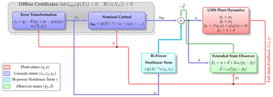
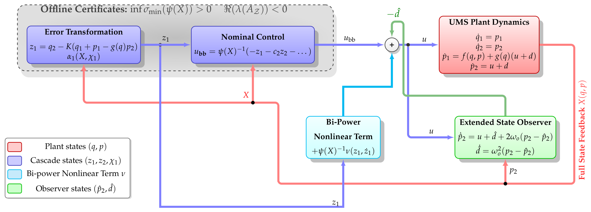
The complete architecture is depicted in Figure 1.

Figure 1. Composite backstepping architecture.

4. Stability Analysis

Lemma 4 (Observer Estimation Bound).

If $\parallel \dot{d}{\left(t\right)\parallel }_2\le {\overline{d}}_1$, the perturbation estimation error $\tilde{d}:=d-\widehat{d}$ satisfies $\underset{t\to \infty }{\mathrm{lim\; sup}}{\parallel \tilde{d}\left(t\right)\parallel }_2\le {\displaystyle \frac{2{\overline{d}}_1}{{\omega }_o}}$.

Proof. 

Defining ${\tilde{p}}_2:=p_2-{\widehat{p}}_2$ and $\tilde{d}:=d-\widehat{d}$, (1) and (10) yield the LTI error dynamics $\dot{E}=A_{o}E+B_o\dot{d}\left(t\right)$, where $E:=\mathrm{col}({\tilde{p}}_2,\tilde{d})$, $B_o:=\mathrm{col}(0,I)$, and $A_o=\left[\begin{array}{cc}-2{\omega }_{o}I& I\\ -{\omega }_o^{2}I& 0\end{array}\right].$

Since all block matrices in $A_o$ are scalar multiples of the identity matrix $I_{n_2}$, each component pair $({\tilde{p}}_{2,i},{\tilde{d}}_i)$ obeys identical dynamics; the transfer function from ${\dot{d}}_i$ to ${\tilde{d}}_i$ is

$$H\left(s\right)={\displaystyle \frac{s+2{\omega }_o}{{(s+{\omega }_o)}^2}},$$

with impulse response $h\left(t\right)=(1+{\omega }_{o}t)e^{-{\omega }_{o}t}\ge 0,\forall t\ge 0$.

Since the impulse response is nonnegative ($h\left(t\right)\ge 0$), the integral form of the triangle inequality and the absolute homogeneity of the Euclidean norm permit the scalar weight to pass through the norm. Accounting for the unforced initial-condition response, the complete error norm satisfies

$$\parallel \tilde{d}{\left(t\right)\parallel }_2\le {∥\left[\begin{array}{cc}0& I\end{array}\right]e^{A_{o}t}E\left(0\right)∥}_2+{\int }_0^{t}h(t-\tau ){\parallel \dot{d}\left(\tau \right)\parallel }_{2}d\tau .$$

Since $A_o$ is Hurwitz [36], the transient term exponentially vanishes as $t\to \infty$. Bounding the remaining convolution integral yields the ultimate limit: $\underset{t\to \infty }{\mathrm{lim\; sup}}{\parallel \tilde{d}\left(t\right)\parallel }_2\le {\overline{d}}_1{\int }_0^{\infty }h\left(\tau \right)d\tau ={\displaystyle \frac{2{\overline{d}}_1}{{\omega }_o}}.$ □

Lemma 5 (Finite-time entrance).

Let $y:{\mathbb{R}}_{\ge 0}\to {\mathbb{R}}^m$ satisfy

$$\ddot{y}=-b_1{\mathrm{sig}}^{\alpha }\left(\dot{y}\right)-b_2{\mathrm{sig}}^{\beta }\left(\dot{y}\right)+\phi \left(t\right),$$

where ${\parallel \phi \left(t\right)\parallel }_2\le \overline{\phi }$, $b_1,b_2>0$, and $0<\alpha <1<\beta$.

• Set $s:=\parallel \dot{y}{\parallel }_2,s_{★}:={\left({\displaystyle \frac{2\overline{\phi }}{b_1}}\right)}^{1/\alpha }.$ Then, for almost every t such that $s\left(t\right)\ge s_{★}$, $\dot{s}\left(t\right)\le -{\displaystyle \frac{b_1}{2}}s{\left(t\right)}^{\alpha }.$ Consequently, if $s\left(0\right)>s_{★}$, then $s\left(t\right)\le s_{★}$ for all $t\ge T_{★}$, where

  $$T_{★}={\displaystyle \frac{2\left(s{\left(0\right)}^{1-\alpha }-s_{★}^{1-\alpha }\right)}{b_1(1-\alpha )}}.$$

Proof. 

For $s>0$, the map $t\mapsto \parallel \dot{y}{\left(t\right)\parallel }_2$ is differentiable almost everywhere, yielding the time derivative $\dot{s}=s^{-1}{\dot{y}}^{\top }\ddot{y}$. By the element-wise definition of the ${\mathrm{sig}}^{\alpha }$ operator, ${\dot{y}}^{\top }{\mathrm{sig}}^{\alpha }\left(\dot{y}\right)={\parallel \dot{y}\parallel }_{\alpha +1}^{\alpha +1}$. Since $\alpha +1\in (1,2)$, the standard inclusion property of finite-dimensional ${\mathcal{l}}_p$ norms implies ${\parallel \dot{y}\parallel }_{\alpha +1}\ge {\parallel \dot{y}\parallel }_2=s$. Consequently,

$${\dot{y}}^{\top }{\mathrm{sig}}^{\alpha }\left(\dot{y}\right)\ge s^{\alpha +1}.$$

The Cauchy–Schwarz inequality and the uniform bound on $\phi$ yield ${\dot{y}}^{\top }\phi \le \parallel \dot{y}{\parallel }_2{\parallel \phi \parallel }_2\le s\overline{\phi }$. Substituting the dynamics of $\ddot{y}$ into the expression for $\dot{s}$ and discarding the nonnegative term $b_2{\dot{y}}^{\top }{\mathrm{sig}}^{\beta }\left(\dot{y}\right)=b_2{\parallel \dot{y}\parallel }_{\beta +1}^{\beta +1}\ge 0$ establishes the differential inequality

$$\dot{s}\le -b_1{s}^{\alpha }+\overline{\phi }.$$

Integrating this inequality via the comparison principle [18] yields the stated entrance time $T_{★}$. □

Assumption 3 (Robust compact containment).

Let $x_a:=\mathrm{col}(X,{\chi }_1)\in {\mathbb{R}}^{2n_1+3n_2}$, and $V_{\mathrm{nom}}:{\mathbb{R}}^{2n_1+3n_2}\mapsto {\mathbb{R}}_{\ge 0}\in C^1$ be a Lyapunov function for the nominal closed-loop system. There exists a constant $c>0$ such that the compact sublevel set ([17], Chapter 4)

$${\mathrm{\Omega }}_a:=\{x_a\mid V_{\mathrm{nom}}\left(x_a\right)\le c\}$$

is strictly contained within the domain of attraction of the nominal equilibrium. Furthermore, there exists a uniform bound ${\overline{\tilde{d}}}_{\sup }>0$ such that, for all $x_a\in \partial {\mathrm{\Omega }}_a$ and all observer errors satisfying $\parallel \tilde{d}{\parallel }_2\le {\overline{\tilde{d}}}_{\sup }$, the following strict dissipation inequality holds:

$$\begin{array}{c}\hfill \nabla V_{\mathrm{nom}}{\left(x_a\right)}^{\top }\mathcal{G}\left(q\right)\left(\psi {\left(X\right)}^{-1}\nu (z_1,{\dot{z}}_1)+\tilde{d}\right)<-\nabla V_{\mathrm{nom}}{\left(x_a\right)}^{\top }{F}_{\mathrm{nom}}\left(x_a\right),\end{array}$$

where $F_{\mathrm{nom}}\left(x_a\right)$ is the nominal closed-loop vector field, and the input distribution matrix is defined as the block column vector

$$\mathcal{G}\left(q\right):=\mathrm{col}(0_{n_1\times n_2},g\left(q\right),0_{n_2\times n_2},I_{n_2},0_{n_2\times n_2}).$$

Theorem 2 (Conditional robust containment and practical entrance).

Suppose the decoupling and local zero-dynamics tests succeed. Let a compact sublevel set ${\mathrm{\Omega }}_a$ have its physical-state projection contained in $\mathrm{int}{\mathrm{\Omega }}_X$, and suppose the robust boundary test in Section 2.6 has been verified for an observer-error budget $E_{\max }$.

Assume that the disturbance and initial observer errors satisfy

$$E_{\sup }\le E_{\max },$$

where $E_{\sup }$ is given by (12). Assume also that actuator saturation is either excluded on the certified set or included explicitly in the verified boundary and residual bounds. For noisy state feedback outside the ESO, the associated controller perturbations must additionally be included in those bounds.

Then, every solution starting in ${\mathrm{\Omega }}_a$ remains in ${\mathrm{\Omega }}_a$ and admits continuation for all $t\ge 0$. For every $\epsilon >0$, the transformed velocity error enters the set specified in Proposition 3 no later than $t_o\left(\epsilon \right)+T_{\mathrm{ent}}$. No finite-time convergence of the complete state to the origin is asserted.

Proof. 

Proposition 2 supplies the required observer-error bound for the entire transient, not only asymptotically. The verified boundary inequality therefore makes the vector field strictly inward pointing on $\partial {\mathrm{\Omega }}_a$. This establishes forward invariance. The bounded disturbance, bounded physical and integral states, and bounded observer errors preclude a finite escape of the augmented solution. The residual bounds and the entrance claim follow from Proposition 3. □

Remark 1 (Explicit residual bound).

Let ${\overline{z}}_i=\underset{x_a\in {\mathrm{\Omega }}_a}{\sup }{\parallel z_i\parallel }_2$, ${\overline{\chi }}_1=\underset{x_a\in {\mathrm{\Omega }}_a}{\sup }{\parallel {\chi }_1\parallel }_2$, $\overline{\psi }={\sup }_{{\mathrm{\Omega }}_X}{\parallel \psi \left(X\right)\parallel }_2$, and let $\overline{\tilde{d}}$ be the bound from Lemma 4. Then,

$$\underset{t\to \infty }{\mathrm{lim\; sup}}{\parallel r\left(t\right)\parallel }_2\le \overline{\psi }\overline{\tilde{d}}+\left|C_1\right|{\overline{z}}_1+\left|C_2\right|{\overline{z}}_2+\lambda c_1{\overline{\chi }}_1\overline{r}.$$

5. Simulation Results

The numerical study follows the protocol in Section 3. Offline algebraic tests on the declared box ${\mathrm{\Omega }}_X$ are reported first; closed-loop records are reported afterwards. A successful analytical or interval certificate and a successful simulation are distinct outcomes. Three implementations share the same plant, the same ${\mathrm{\Omega }}_X$, the same $T_b$ and the same coefficients: the nominal law in (2) (BB), that law with (10) (BB+ESO), and the composite law in (16) (BB+ESO+FT).

5.1. Plant, Box and Implemented Coefficients

The plant is a virtual replica of the Digital Pendulum System (Feedback Instruments, model 33-005-PCI) ([16], Section 4.6). Parameters and the design box

$${\mathrm{\Omega }}_X=\left\{X=\mathrm{col}(x,\theta ,v,\omega ):\left|x\right|\le \overline{x},\left|\theta \right|\le \overline{\theta },\left|v\right|\le \overline{v},\left|\omega \right|\le \overline{\omega }\right\}$$

are listed in Table 1. Here, $n_1=n_2=1$ and $K=k$. As in Section 2.5, the matched signal d lives in the partially linearised acceleration channel. A physical force $F_d$ satisfies $d=F_d/(M+m{\sin }^2\theta )$ on the exact model, so a bound on ${\dot{F}}_d$ is not, by itself, a bound on $\dot{d}$.

Table 1. Cart–pendulum parameters and design box ${\mathrm{\Omega }}_X$. Inertias follow $J_{\mathrm{com}}=J_p-m{\mathcal{l}}^2$. Friction and the force/rail limits are modelling assumptions of the virtual replica.

Quantity	Symbol	Value	Unit
Cart mass	M	$2.4$	$\mathrm{kg}$
Pendulum mass	m	$0.23$	$\mathrm{kg}$
Pivot to centre of mass	ℓ	$0.36$	$\mathrm{m}$
Pivot inertia	$J_p$	$0.039744$	$\mathrm{kg}{\mathrm{m}}^2$
Centre-of-mass inertia	$J_{\mathrm{com}}$	$0.009936$	$\mathrm{kg}{\mathrm{m}}^2$
Cart viscous friction	$b_x$	$0.05$	$\mathrm{N}\mathrm{s}{\mathrm{m}}^{-1}$
Pivot viscous damping	$b_{\theta }$	$0.001$	$\mathrm{N}\mathrm{m}\mathrm{s}{\mathrm{rad}}^{-1}$
Gravity	$g_0$	$9.81$	$\mathrm{m}{\mathrm{s}}^{-2}$
Actuator force limit	$F_{\max }$	15	$\mathrm{N}$
Rail half-travel (safety)	—	$0.45$	$\mathrm{m}$
Cart/angle bounds	$\overline{x},\overline{\theta }$	$0.25,0.25$	$\mathrm{m}$, $\mathrm{rad}$
Velocity bounds	$\overline{v},\overline{\omega }$	$0.50,1.50$	$\mathrm{m}{\mathrm{s}}^{-1}$, $\mathrm{rad}{\mathrm{s}}^{-1}$

Implemented gains appear in Table 2. In particular, ${\omega }_o=30{\mathrm{s}}^{-1}$ and $(b_1,b_2)=(0.879,0.621)\mathrm{m}{\mathrm{s}}^{-2}$. The cascade pair satisfies $c_1+c_2=8{\mathrm{s}}^{-1}$, whence $C_1=1-c_1^2+\lambda =-6.838$ and $C_2=8$. The bi-power term is evaluated on the normalised arguments $z_1/z_{\mathrm{ref}}$ and ${\dot{z}}_1/s_{\mathrm{ref}}$ rather than on $z_1,{\dot{z}}_1$ directly. Because ${\mathrm{sig}}^{\rho }$ is homogeneous of degree $\rho$, this is a rescaling of (15): the tabulated $(a_i,b_i)$ and the comparison time $T_{\mathrm{formula}}$ belong to those normalised coordinates, which are also the coordinates in which Proposition 3 is applied.

Table 2. Implemented controller and offline numbers at the selected k. The pair $(c_1,c_2)$ is the split of $c_1+c_2=8$ used in the code. The weights $(a_i,b_i)$ and $T_{\mathrm{formula}}$ are those of the normalised bi-power term.

Quantity	Symbol	Value	Unit
Transformation time scale	$T_b$	$0.15$	$\mathrm{s}$
Transformation gain	k	$-0.910$	$\mathrm{m}{\mathrm{rad}}^{-1}$
Cascade gains	$c_1,c_2$	$3.324,4.676$	${\mathrm{s}}^{-1}$
Integral gain	$\lambda$	$3.208$	${\mathrm{s}}^{-2}$
Observer bandwidth	${\omega }_o$	30	${\mathrm{s}}^{-1}$
Homogeneity exponents	$\alpha ,\beta$	$0.6,1.4$	—
Position FT weights	$a_1,a_2$	$0.20,0.05$	$\mathrm{m}{\mathrm{s}}^{-2}$
Velocity FT weights	$b_1,b_2$	$0.879,0.621$	$\mathrm{m}{\mathrm{s}}^{-2}$
Position/velocity references	$z_{\mathrm{ref}},s_{\mathrm{ref}}$	$0.10,0.30$	$\mathrm{m}$, $\mathrm{m}{\mathrm{s}}^{-1}$
Certified decoupling lower bound	$\underline{\sigma }$	$0.652$	—
Local zero-dynamics margin	${\mu }_{\mathcal{Z}}$	$3.254$	${\mathrm{s}}^{-1}$
Transformation Jacobian lower bound	$H_{\min }$	$0.894$	—
Conditional FT comparison time	$T_{\mathrm{formula}}$	$2.91$	$\mathrm{s}$

Integrations use RK4 with $\mathrm{d}t=1\mathrm{ms}$ on a horizon of $T=8\mathrm{s}$. A step-halving check on the same vector field, controller and noise functions produced a four-state discrepancy no larger than $1.5\times {10}^{-6}$ in SI units.

The actuator is limited to $F_{\max }=15\mathrm{N}$. Lemma 3 holds with ${\delta }_u=0$ only when $u_a=u_c$. In the numerical plant, the requested force is clipped, and the observer is fed $u_a$ rather than $u_c$. Across the records below, the observed saturation fraction is either zero or of order ${10}^{-3}$ of the horizon. That sampled fact does not replace the set-wise test in Section 2.6.

5.2. Offline Tests of $\psi$ and $A_{\mathcal{Z}}$

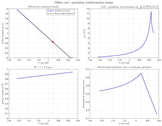
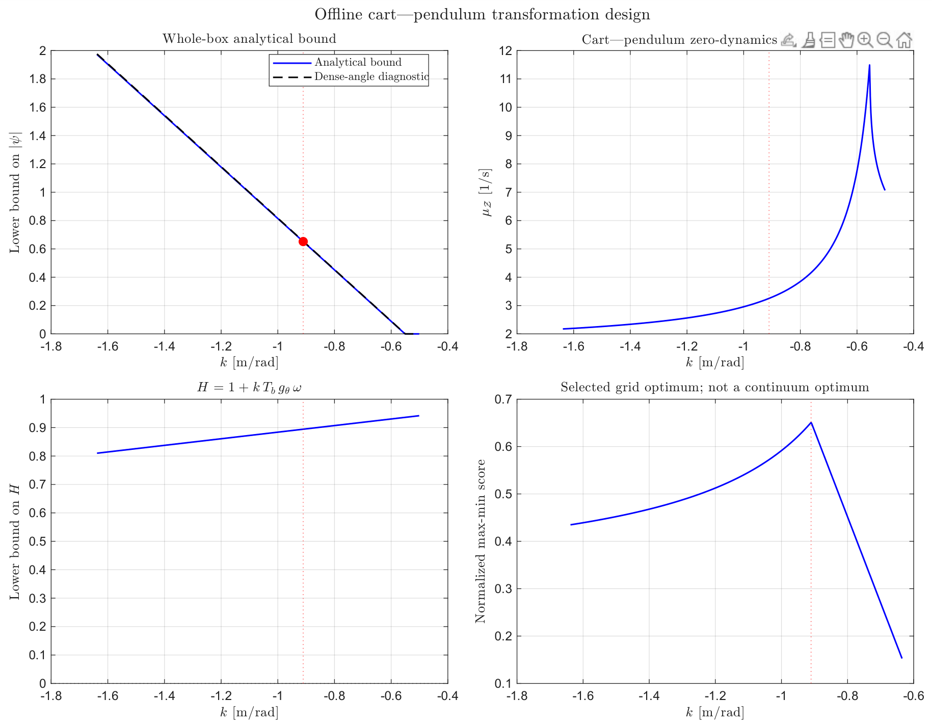
For this plant, $\psi$ is the scalar from Section 2.5. Figure 2 plots the whole-box analytical lower bound $\left|\psi \right|\ge \left|k\right|L_B-1$ against k, together with a dense-angle diagnostic. The two curves agree on the plotted interval. The diagnostic is not a substitute for the verified covering argument in Proposition 1; it is reported as a check on the conservative closed-form bound. Because $\psi$ is scalar, the calculation is cheap. For larger n, the same test must be replaced by the box-covering procedure from Section 2.

Figure 2. Offline transformation design on ${\mathrm{\Omega }}_X$.

The marker $k=-0.910\mathrm{m}{\mathrm{rad}}^{-1}$ is the maximiser of a normalised max–min score on a declared finite grid, not a continuum optimiser. At that value, the design script returns

$$\underline{\sigma }=0.652,{\mu }_{\mathcal{Z}}=-\underset{i}{\max }\mathrm{Re}{\lambda }_i\left(A_{\mathcal{Z}}\right)=3.254{\mathrm{s}}^{-1},H_{\min }=0.894,\det J_{\xi }=1.$$

Thus, $J_{\xi }$ is nonsingular and the implemented $A_{\mathcal{Z}}$ is Hurwitz with spectral abscissa $-{\mu }_{\mathcal{Z}}$. The two eigenvalues are the roots of that same implemented $2\times 2$ matrix, assembled by (5) in the coordinates of the numerical model. They are not inferred from the point-mass specialisation in Section 2.5 unless that specialisation is the model used in code: the virtual replica uses $J_p$, whereas the displayed point-mass Jacobian uses $m{l}^2$.

The top-left panel in Figure 2 is a lower bound on $\left|\psi \right|$. It does not give $\overline{\psi }={\sup }_{X\in {\mathrm{\Omega }}_X}{\parallel \psi \left(X\right)\parallel }_2$, which is a separate upper estimate at the selected k. On the recorded orbits of the next subsections, $\left|\psi \right|$ remains near $0.89$. Residual quantities $\overline{r}$ and $\overline{\phi }$ in the sense of the explicit residual bound and of Proposition 3 further require extrema of $(z_1,z_2,{\chi }_1)$ on a declared ${\mathrm{\Omega }}_a$. Those extrema are not read from a single trajectory, and they are not claimed here as verified set-wise bounds.

5.3. Observer Envelope and Decoupling Along One Record

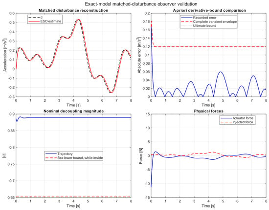
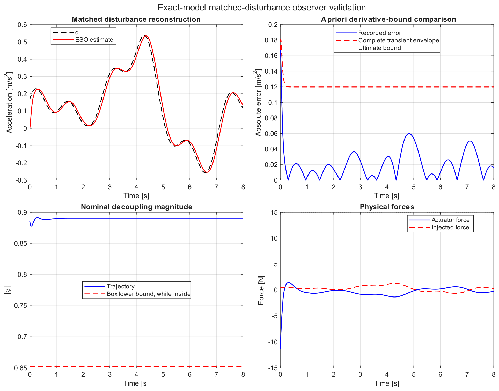
Lemma 4 is an ultimate bound. Theorem 2 uses the complete transient budget of Proposition 2. Figure 3 shows both, for the injected acceleration-channel signal of this campaign (not the force-rate figure of an earlier draft). The ultimate line in the figure is $2{\overline{d}}_1/{\omega }_o$ at the implemented ${\omega }_o=30{\mathrm{s}}^{-1}$ and at the rate bound of that same injected d. After about $0.2\mathrm{s}$, the recorded $|\tilde{d}|$ lies below that line; the first samples do not. Forward invariance of a candidate ${\mathrm{\Omega }}_a$ on this record is therefore an observed property of the initialisation, not a corollary of the limsup alone.

Figure 3. Exact–model observer record.

Along the same orbit, $\left|\psi \right|$ remains near $0.89$, above $\underline{\sigma }=0.652$, whilst the state stays inside ${\mathrm{\Omega }}_X$. Requested and injected forces are plotted together so that any approach to $F_{\max }$ can be seen. On this record the applied force stays inside the limiter after the opening sample.

5.4. One Common Stress Comparison

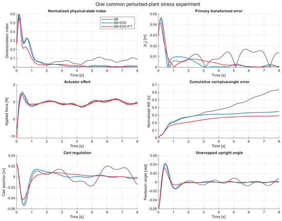
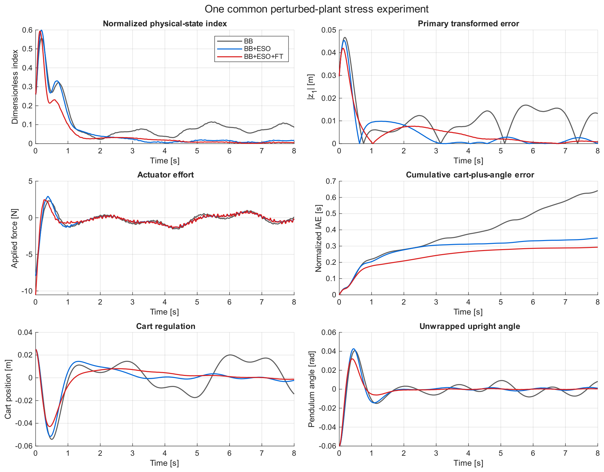
A single Lipschitz disturbance and a common initial condition are applied to all three laws (Figure 4, Table 3). BB leaves a persistent oscillation. BB+ESO removes most of that residual. BB+ESO+FT further reduces $|z_1|$ after the first second and records the smallest terminal index and the smallest IAE on this horizon. Settling times are $1.06\mathrm{s}$ (BB+ESO) and $0.97\mathrm{s}$ (BB+ESO+FT); BB does not meet the settling test in $8\mathrm{s}$. The minimum observed $\left|\psi \right|$ is $0.878$.

Figure 4. Common perturbed–plant experiment.

Table 3. Quantitative comparison. Stress: one common disturbance and initial condition (seed 73). Monte Carlo: median (minimum, maximum) over 24 shared seeds. BB settling statistics use the 21 records that settle. IAE_x in metre-seconds; IAE_θ in radian-seconds.

Record	Metric	BB	BB+ESO	BB+ESO+FT
Stress	Settle [s]	—	$1.06$	$0.97$
	IAEx [$\mathrm{m}\mathrm{s}$]	$0.105$	$0.051$	$0.049$
	IAEθ [$\mathrm{rad}\mathrm{s}$]	$0.055$	$0.036$	$0.025$
	Norm. IAE [s]	$0.642$	$0.350$	$0.293$
	RMS force [N]	$1.05$	$1.08$	$1.08$
	Min. $\left|\psi \right|$	$0.879$	$0.878$	$0.878$
	Peak domain ratio	$0.505$	$0.540$	$0.527$
	Terminal index	$0.086$	$0.018$	$0.006$
Monte Carlo	Completed/success	$24/24$,$21/24$	$24/24$,$24/24$	$24/24$,$24/24$
	Settle [s]	$5.07(0.29,7.39)$	$1.07(0.27,2.12)$	$0.87(0.20,2.19)$
	Norm. IAE [s]	$0.618(0.362,1.094)$	$0.295(0.104,0.680)$	$0.234(0.074,0.650)$
	RMS force [N]	$0.877(0.502,1.628)$	$0.838(0.470,1.653)$	$0.848(0.470,1.650)$
	Min. $\left|\psi \right|$	$0.885(0.863,0.889)$	$0.885(0.862,0.888)$	$0.885(0.860,0.889)$
	Peak domain ratio	$0.326(0.118,0.960)$	$0.336(0.118,0.987)$	$0.333(0.113,0.996)$

Two caveats belong here. First, the record is not a proof of Theorem 2, and the figure does not display $T_{\mathrm{ent}}$. The comparison time associated with Proposition 3, after a residual radius has been sampled a posteriori in the normalised coordinates of Table 2, is $T_{\mathrm{formula}}=2.91\mathrm{s}$. The last entry of $|{\dot{z}}_1|$ into the engineering band on the recorded family occurs earlier than that mark. Second, total variation of the applied force is larger for BB+ESO+FT than for BB+ESO ($57.5\mathrm{N}$ against $34.7\mathrm{N}$ on this record). The bi-power term buys IAE and terminal error at the price of a more lively actuator.

5.5. Seeded Monte Carlo

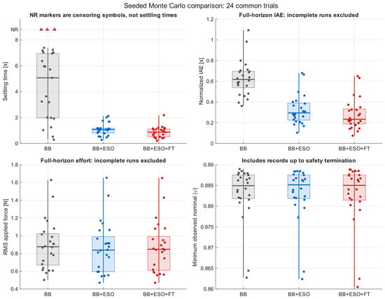
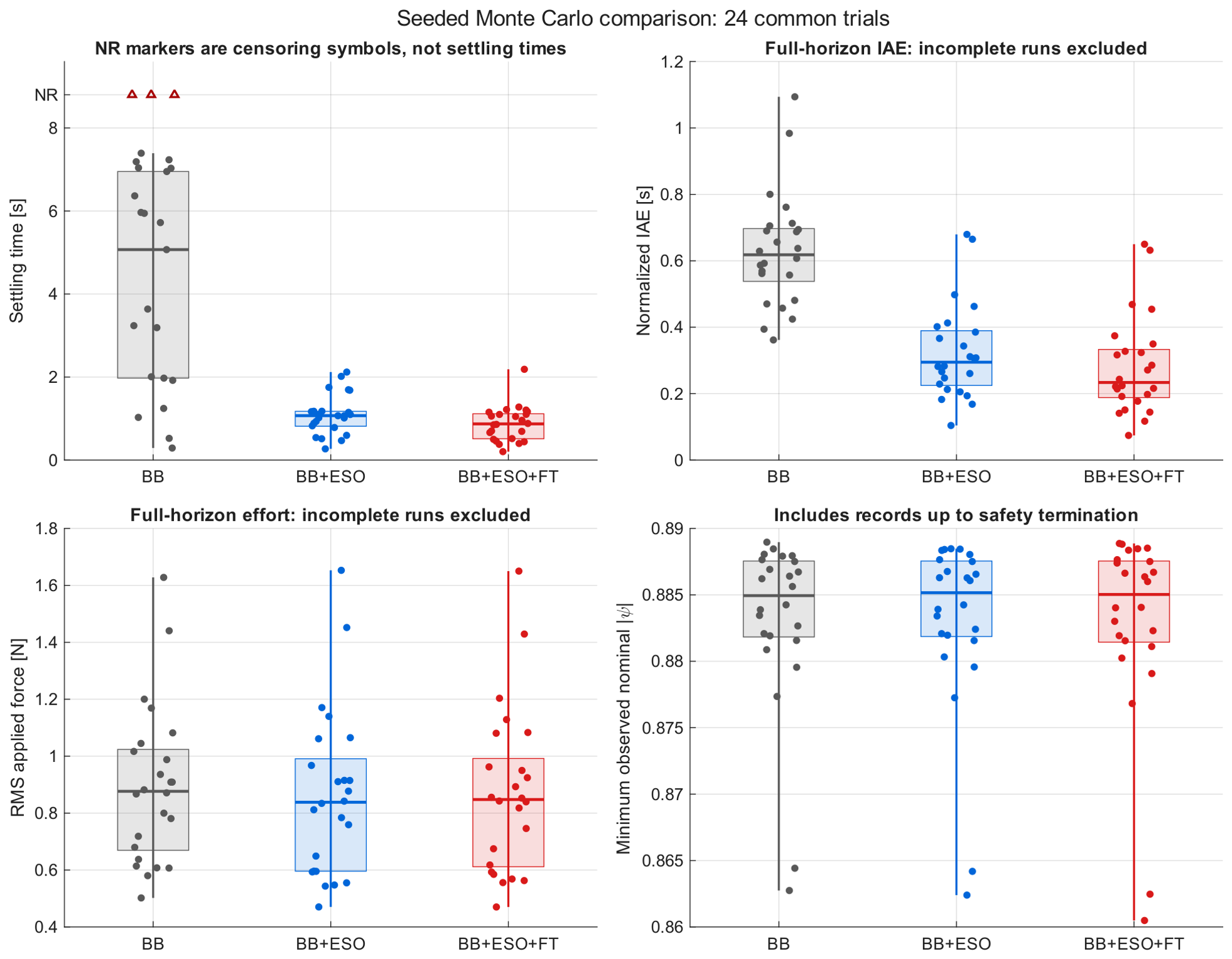
Twenty-four common seeds are reused for the three controllers (Figure 5, Table 3). Every run completed $8\mathrm{s}$. Under a strict success test combining settling, terminal index and box containment, BB succeeds on $21/24$ seeds (3 censored non-settling records, not crashes); BB+ESO and BB+ESO+FT succeed on $24/24$. Median settling times fall from $5.07\mathrm{s}$ (BB, on those records that settle) to $1.07\mathrm{s}$ and $0.87\mathrm{s}$. Median normalised IAE falls from $0.618$ to $0.295$ and $0.234$. Median RMS force is essentially unchanged (≈0.84–0.88 $\mathrm{N}$); total variation is systematically higher once the bi-power term is active.

Figure 5. Seeded Monte Carlo on 24 common trials. Settling-time NR markers are censored BB records, not numerical settling times. IAE and RMS force use completed horizons only (all runs completed). Minimum observed $\left|\psi \right|$ includes records up to any safety stop. The overlays improve settling and IAE; they do not reduce RMS effort.

The smallest $\left|\psi \right|$ among all 72 records is $0.860$, still above ${\sigma }_{★}$. The largest peak domain ratio is $0.996$, so no sampled orbit leaves ${\mathrm{\Omega }}_X$. These are counts from a finite seeded study. They are not hypothesis tests, not empirical probabilities of stability, and not a covering of ${\mathrm{\Omega }}_X$. In the language of Section 2.6, they do not replace the interval boundary test in Assumption 3.

No finite-time convergence of $(X,{\chi }_1,{\widehat{p}}_2,\widehat{d})$ to the origin is inferred from any of the four figures. Additional diagnostics generated on the same campaign (nominal regulation, phase portraits, a sampled quadratic that is not a containment certificate, a velocity-entrance family, completion counts, a four-term anatomy of $\nu$, and the step-refinement overlay) are omitted from the main text.

6. Conclusions

The offline tests decide the invertibility of $\psi$ on ${\mathrm{\Omega }}_X$ and local exponential stability of the zero dynamics. Both are properties of a declared model and a declared compact set: a completed covering with $\underline{\sigma }>0$ gives ${\sigma }_{★}\ge \underline{\sigma }$ and a usable inverse bound. A Hurwitz Jacobian $A_{\mathcal{Z}}$ is a local statement about the unforced zero dynamics. It is not a robustness certificate for the perturbed loop.

The overlays address that gap only in the sense made precise by Theorem 2. The observer contributes the ultimate bound $2{\overline{d}}_1/{\omega }_o$ and the transient budget $E_{\sup }$ used in the invariance argument. The bi-power term contributes the entrance time $t_o\left(\epsilon \right)+T_{\mathrm{ent}}$ for $\parallel {\dot{z}}_1{\parallel }_2$. Neither overlay is claimed to render the full state $(X,{\chi }_1,{\widehat{p}}_2,\widehat{d})$ finite-time stable. The cart–pendulum records in Section 5 are consistent with those distinctions; they are not a covering of Assumption 3. The construction remains the block-backstepping law of [15], with the tests and overlays attached.

References

- Lu, B.; Fang, Y. Online trajectory planning control for a class of underactuated mechanical systems. IEEE Trans. Autom. Control 2024, 69, 442–448. [Google Scholar] [CrossRef] [Scilit]
- Reyhanoglu, M.; van der Schaft, A.; McClamroch, N.H.; Kolmanovsky, I. Dynamics and Control of a Class of Underactuated Mechanical Systems. IEEE Trans. Autom. Control 1999, 44, 1663–1671. [Google Scholar] [CrossRef] [Scilit]
- Wang, B.; Nersesov, S.; Ashrafiuon, H. Quasi-LPV Control Design for a Class of Underactuated Mechanical Systems. In Proceedings of the 2022 American Control Conference (ACC), Atlanta, GA, USA, 8–10 June 2022; pp. 1904–1909. [Google Scholar] [CrossRef] [Scilit]
- Franco, E.; Arpenti, P.; Donaire, A.; Ruggiero, F. Integral IDA-PBC for Underactuated Mechanical Systems Subject to Matched and Unmatched Disturbances. IEEE Control Syst. Lett. 2024, 8, 568–573. [Google Scholar] [CrossRef] [Scilit]
- Emirsajłow, Z.; Barciński, T. A Robust Asymptotic Tracking Controller for an Uncertain 2DOF Underactuated Mechanical System Motivated by a Satellite Attitude Control Problem. Int. J. Appl. Math. Comput. Sci. 2025, 35, 97–116. [Google Scholar] [CrossRef] [Scilit]
- Krafes, S.; Chalh, Z.; Saka, A. A Review on the Control of Second Order Underactuated Mechanical Systems. Complexity 2018, 2018, 9573514, Correction in Complexity 2020, 2020, 1629749. https://doi.org/10.1155/2020/1629749. [Google Scholar] [CrossRef] [Scilit]
- Liu, Y.; Yu, H. A Survey of Underactuated Mechanical Systems. IET Control Theory Appl. 2013, 7, 921–935. [Google Scholar] [CrossRef] [Scilit]
- Huang, Z.; Yu, C.; Zeng, B.; Gong, X.; Zhou, H. A Survey of Planar Underactuated Mechanical System. Machines 2024, 12, 829. [Google Scholar] [CrossRef] [Scilit]
- Olfati-Saber, R. Normal forms for underactuated mechanical systems with symmetry. IEEE Trans. Autom. Control 2002, 47, 305–308. [Google Scholar] [CrossRef] [Scilit]
- Fantoni, I.; Lozano, R. Non-Linear Control for Underactuated Mechanical Systems; Springer: London, UK, 2001. [Google Scholar] [CrossRef] [Scilit]
- Xin, X.; Liu, Y. Control Design and Analysis for Underactuated Robotic Systems; Springer: London, UK, 2014. [Google Scholar] [CrossRef] [Scilit]
- Olfati-Saber, R. Cascade Normal Forms for Underactuated Mechanical Systems. In Proceedings of the 39th IEEE Conference on Decision and Control, Sydney, Australia, 12–15 December 2000; pp. 2162–2167. [Google Scholar] [CrossRef] [Scilit]
- Olfati-Saber, R. Nonlinear Control and Reduction of Underactuated Systems with Symmetry. II. Unactuated Shape Variables Case. In Proceedings of the Proceedings of the 40th IEEE Conference on Decision and Control, Orlando, FL, USA, 4–7 December 2001; pp. 4164–4169. [Google Scholar] [CrossRef] [Scilit]
- Li, N.; Liu, X.; Liu, C.; Wang, H.; Ju, J.; Li, C. A novel block backstepping-based trajectory tracking control with zero dynamics stability for underactuated overhead cranes. ISA Trans. 2025, 166, 379–392. [Google Scholar] [CrossRef] [Scilit]
- Rudra, S.; Barai, R.K.; Maitra, M. Nonlinear State Feedback Controller Design for Underactuated Mechanical System: A Modified Block Backstepping Approach. ISA Trans. 2014, 53, 317–326. [Google Scholar] [CrossRef] [Scilit]
- Rudra, S.; Barai, R.K.; Maitra, M. Block Backstepping Design of Nonlinear State Feedback Control Law for Underactuated Mechanical Systems; Springer: Singapore, 2017. [Google Scholar] [CrossRef] [Scilit]
- Khalil, H. Nonlinear Systems; Pearson Education, Prentice Hall: Upper Saddle River, NJ, USA, 2002. [Google Scholar]
- Hahn, W. Stability of Motion; Grundlehren der Mathematischen Wissenschaften; Springer: Berlin/Heidelberg, Germany, 2012. [Google Scholar] [CrossRef] [Scilit]
- Krstic, M.; Kokotovic, P.V.; Kanellakopoulos, I. Nonlinear and Adaptive Control Design, 1st ed.; John Wiley & Sons, Inc.: Hoboken, NJ, USA, 1995. [Google Scholar]
- Farrell, J.A.; Polycarpou, M.; Sharma, M.; Dong, W. Command Filtered Backstepping. IEEE Trans. Autom. Control 2009, 54, 1391–1395. [Google Scholar] [CrossRef] [Scilit]
- Ye, H.; Song, Y. Backstepping Design Embedded With Time-Varying Command Filters. IEEE Trans. Circuits Syst. II Express Briefs 2022, 69, 2832–2836. [Google Scholar] [CrossRef] [Scilit]
- Zhu, J.; Li, S.; Liu, Z. Adaptive command filter control for switched time-delay systems with dead-zone based on an exact disturbance observer. Int. J. Robust Nonlinear Control 2024, 34, 10131–10159. [Google Scholar] [CrossRef] [Scilit]
- Xu, D.; Dai, Y.; Yang, C.; Yan, X. Adaptive fuzzy sliding mode command-filtered backstepping control for islanded PV microgrid with energy storage system. J. Frankl. Inst. 2019, 356, 7025–7046. [Google Scholar] [CrossRef] [Scilit]
- Mercorelli, P. Feedforward and repetitive control of a servo piezo-mechanical hydraulic actuator. J. Phys. Conf. Ser. 2020, 1564, 012005. [Google Scholar] [CrossRef] [Scilit]
- Turrisi, G.; Capotondi, M.; Gaz, C.; Modugno, V.; Oriolo, G.; De Luca, A. On-Line Learning for Planning and Control of Underactuated Robots with Uncertain Dynamics. IEEE Robot. Autom. Lett. 2022, 7, 358–365. [Google Scholar] [CrossRef] [Scilit]
- Turcato, N.; Calì, M.; Dalla Libera, A.; Giacomuzzo, G.; Carli, R.; Romeres, D. Learning Global Control of Underactuated Systems with Model-Based Reinforcement Learning. arXiv 2025, arXiv:2504.06721. [Google Scholar] [CrossRef] [Scilit]
- Royden, H.; Fitzpatrick, P. Real Analysis; Pearson Modern Classics for Advanced Mathematics Series; Pearson: London, UK, 2018. [Google Scholar]
- Horn, R.A.; Johnson, C.R. Matrix Analysis, 2nd ed.; Cambridge University Press: Cambridge, UK, 2012. [Google Scholar] [CrossRef] [Scilit]
- Moore, R.E.; Kearfott, R.B.; Cloud, M.J. Introduction to Interval Analysis; Society for Industrial and Applied Mathematics: Philadelphia, PA, USA, 2009. [Google Scholar] [CrossRef] [Scilit]
- Boyd, S.; Vandenberghe, L. Convex Optimization; Cambridge University Press: Cambridge, UK, 2004. [Google Scholar] [CrossRef] [Scilit]
- Krantz, S.G.; Parks, H.R. The Implicit Function Theorem: History, Theory, and Applications; Birkhäuser: Boston, MA, USA, 2002. [Google Scholar] [CrossRef] [Scilit]
- Teschl, G. Ordinary Differential Equations and Dynamical Systems; American Mathematical Society: Providence, RI, USA, 2012; Volume 140. [Google Scholar]
- Le, D.T.; Dao, Q.T. A model-assisted ESO-based nonlinear ADRC for robust transportation control of a biglide parallel robot. Results Control Optim. 2026, 24, 100761. [Google Scholar] [CrossRef] [Scilit]
- Zhu, W.; Du, H. Global Uniform Finite-Time Output Feedback Stabilization for Disturbed Nonlinear Uncertain Systems: Backstepping-like Observer and Nonseparation Principle Design. SIAM J. Control Optim. 2024, 62, 1717–1736. [Google Scholar] [CrossRef] [Scilit]
- Dao, K.L.; Tran, M.K.; Tong, T.L.; Duong, M.D. Disturbance observer integrated proportional–derivative sliding mode control for trajectory tracking control of quadrotor UAVs. Results Control Optim. 2026, 24, 100769. [Google Scholar] [CrossRef] [Scilit]
- Guo, B.Z.; Zhao, Z.L. On the convergence of an extended state observer for nonlinear systems with uncertainty. Syst. Control Lett. 2011, 60, 420–430. [Google Scholar] [CrossRef] [Scilit]
- Darouach, M. Complements to full order observer design for linear systems with unknown inputs. Appl. Math. Lett. 2009, 22, 1107–1111. [Google Scholar] [CrossRef] [Scilit]
- Polyakov, A.; Krstic, M. Finite- and Fixed-Time Nonovershooting Stabilizers and Safety Filters by Homogeneous Feedback. IEEE Trans. Autom. Control 2023, 68, 6434–6449. [Google Scholar] [CrossRef] [Scilit]
Disclaimer/Publisher’s Note: The statements, opinions and data contained in all publications are solely those of the individual author(s) and contributor(s) and not of MDPI and/or the editor(s). MDPI and/or the editor(s) disclaim responsibility for any injury to people or property resulting from any ideas, methods, instructions or products referred to in the content. |
© 2026 by the authors. Licensee MDPI, Basel, Switzerland. This article is an open access article distributed under the terms and conditions of the Creative Commons Attribution (CC BY) license.