


Abstract
With the aim of reducing and eventually eliminating CO2 emissions, the aviation industry is investigating alternative fuels, with liquid hydrogen (LH2) being one of the most promising. Several research projects that deal with the subsystem design of liquid hydrogen aircraft have commenced, with specific attention given to the development of lightweight cryogenic tanks. Composite materials are potential candidates for cryogenic aviation applications, yet they experience issues with thermal stresses that result to various types of damage that should be thoroughly investigated, to enable reliable composite cryogenic structures. In this direction, the present work investigates the alternative finite element techniques for the thermo-mechanical analysis of the characteristic geometrical structural configuration. Thermo-mechanical stress analysis results derived from the investigated analysis methodologies are verified by their comparison to published results. The assessment of the alternative modeling techniques contributes to the adaptation of the FE modeling development strategy to the desired analysis type and the expected results and is directly applicable to the thermo-mechanical design of cryogenic components. The outcome of the investigation is demonstrated in the case of thermo-mechanical analysis of an outer tank of an LH2 storage system, performed with the optimal combination of shell and solid elements.
1. Introduction
The use of laminated composites in aerospace applications is constantly increasing [1,2,3]. Composite materials in general offer high specific strength and stiffness values. Their properties can also be tailored according to the needs of each application, as is the case with laminates, where layers with different orientations can be appropriately stacked, in order to reinforce the structure in the direction needed, thus saving weight, manufacturing and operational costs [4,5,6,7,8]. Composite systems consist of two or more different material types, with each one having different properties. In the majority of aerospace applications, fiber composites are used, with glass, aramid or carbon fibers encased within a polymeric matrix. In most applications, the fibers are unidirectional, meaning that the composite has higher strength and stiffness along the direction of the fibers [9,10,11,12]. Although this anisotropic behavior is desirable in most applications, issues arise when composite structures are subjected to thermal loading, in both high- and low-temperature environments. Anisotropy is not limited to the mechanical properties; composites also have anisotropic thermal properties. As the fiber and the matrix have different coefficients of thermal expansion (CTEs), thermo-mechanical stresses are developing when temperature differences are experienced. There are two mechanisms of thermal stress development [13]. The first takes place inside each layer and is caused by the CTE difference between matrix and fibers resulting in the ply level stresses [14]. The second takes place at the laminate level, because the layers of a composite laminate expand or contract in a different manner when compared to their neighboring layers, as the CTEs along each layer direction are different, resulting in intralayer and interlaminar thermal stresses [15], which in many cases can be severe, or even cause failure [16,17,18]. Thermal stresses in composite laminates comprise a critical issue for cryogenic tank design, such as rocket propellant tanks and hydrogen tanks of future cryogenic commercial aircraft. A prominent example is the catastrophic failure of the propellant tank of the X-33 experimental spaceplane, where thermal stresses were the main reason for the tank explosion [19,20].
In this direction, the present work addresses the issue of thermos-mechanical stress analysis using finite element methodologies, with the aim of assessing optimized FE modeling techniques for the development of a global high-fidelity structural model of a cryogenic tank for aircraft applications. Following a review of analytical methodologies for through-the-thickness stress calculation, two finite element modeling techniques are applied, one with shell and one with solid elements, and their results are compared to analytical calculations in the literature. The two methodologies are applied to mechanical and thermal load cases, as well as different geometries, including curved ones. Conclusions are drawn regarding the accuracy of the numerical results of each method under each load case and for each geometry, as well as of their computational efficiency. Subsequently, both analysis approaches are demonstrated in the case of an indicative foam-insulated LH2 tank thermo-mechanical analysis, performed with an optimal combination of shell and solid elements, paving the way for performing high-fidelity reliable thermo-mechanical analysis of cryogenic structures.
2. Literature Review
Several theories have evolved through the years in order to perform stress analyses of composite laminate plates. These theories can be divided into the categories of three-dimensional elasticity, equivalent single layer (ESL), layer-wise (LW) and zig-zag (ZZ) theories [21]. The most basic theories are the ESL, with the first one being the classical laminate plate theory (CLPT). It is an extension of the classical plate theory (CPT) of Kirchhoff [22] that was modified by Love [23]. This theory assumes no change in thickness and no transverse shear deformations under any loads. This theory provided dependable results for slender plates under small deformations. For thicker plates though, results are not accurate as there are significant out-of-plane deformations that should be also considered. The first-order shear deformation theory (FSDT) or Reissner–Mindlin theory removes some of the assumption of the CLPT and allows the rotation of the cross-section of the plate, thus introducing transverse shear deformations, which are considered constant through the thickness, which also implies that shear stresses are constant [24,25]. As per the elementary theory of homogenous beams, the transverse shear stresses vary parabolically through the thickness. The results of the FSDT can be improved with the introduction of shear correction factors. These factors are case-dependent, and they do not always guarantee good accuracy [26]. Many finite element (FE) packages, like ANSYS that is used in the present work, use FSDT variations for their shell element formulations [27]. When higher accuracy is required, higher order theories can be used, which remove even more assumptions of the CLPT. The Vlasov–Reddy third-order shear deformation theory (TSDT) is one of the most prominent [28], while other theories also exist. Advanced higher order theories like the fifth-order shear deformation theory of Ghumare consider the effects of the in-plane strains, further increasing the accuracy of the results [29]. Approximation of the shear deformation with trigonometric functions is also possible, as in the theory developed by Touratier [30]. For improved results under more complex loading conditions, including dynamic and vibration loads, exponential shear deformation theories (ESDTs) like the one developed by Karama, Afaq and Mistou can be used [31]. The ESL theories mentioned above can be applied to each single ply of the laminate separately. As the displacements of each layer should be compatible with the displacements of the adjacent layers, continuity constraints have to be applied. This is the base of the layer-wise theories, which are divided into partial and full layer-wise theories. The accuracy of the layer-wise theories is constrained by the accuracy of the ESL theories that are used, while their complexity significantly increases when laminates with a high number of plies are analyzed. Several LW theories have been developed, with some of the most widely used being the ones of Mau [32], Ren [33] and Reddy [34]. The zig-zag theories are similar to the layer-wise theories, with the main difference being that they are independent of the number of plies of the laminate. The zig-zag theories use a multiple displacement field with multiple approaches on the calculation of deformations [35]. Three-dimensional elasticity theories do not consider a composite laminate as a two-dimensional plate as is the case with the previous theories. The laminate is considered as a three-dimensional body with all deformation effects considered. These theories provide the most accurate results, with their main disadvantage being their high complexity [36].
Thermal stresses in composite laminates is a well understood problem, as the matrix and fibers have different CTEs. Thermal stresses develop by three different mechanisms: (a) in the ply level, due to the CTE mismatch between fiber and matrix, (b) in the laminate level, due to the homogenized CTE (at the ply level) mismatch between the different plies and (c) in the global structural level, due to the thermal properties mismatch of different structural elements that are in thermal contact.
Most studies focus on micromechanical behavior, which can take into account the thermal stresses developing at the ply level due to fiber–matrix property differences [37,38,39]. Residual stresses from manufacturing are also a recognized issue, yet most studies focus only on the micromechanical behavior [40,41,42], with metallic and ceramic matrix composites being among the most analyzed [43,44,45]. Although thermal stresses in composites are widely investigated on a micromechanical scale, and are often conducted using numerical models, studies at higher levels such as the laminated plate and global level that may include different structural element are rare.
Many composite structures that operate under cryogenic conditions are currently under development [46,47,48], with FE simulations being one of the most important tools for their design and structural integrity verification. As micromechanical modeling predictions are not applicable at larger scales, there is a need for a comprehensive study of the applicability of the existing FE modeling methods at larger scales, in order to pave the way for efficient yet accurate full-scale models.
The majority of commercial FE software offers the option between shell elements or solid elements for modeling composite structures. In the case of ANSYS Mechanical APDL 2024 R1 that is used in the present studies, structural shell elements use the Reissner–Mindlin first-order shear deformation theory. Shear correction factors are automatically calculated based on the cross-section and temperature inputs [27]. Shell elements using the more accurate higher order theories are not easily available on such software, as the more complex formulation of these theories requires a high level of customization, as well as more degrees of freedom that significantly increase the computational cost [49]. The availability of three-dimensional elasticity-based solid elements with significantly increased accuracy covers the high accuracy demands, yet at a high computational cost. Therefore, an evaluation of the modeling approach capabilities as a function of their accuracy, for the case of shell and solid elements, is required in order to define modeling strategies, based on the required result accuracy and available computational resources. In the present work, a comparative study between FE models developed with shell elements using the Reissner–Mindlin theory and models with solid elements using the three-dimensional elasticity theory are investigated under various thermal, mechanical and thermo-mechanical loading cases. The results are compared to literature solutions, drawing conclusions about the efficiency and reliability of each approach for the various structural analysis cases, with specific attention given to the effect of the curvature on the accuracy of the results.
3. Considered Finite Element Modeling Methodologies and Materials
The main aim of the present work is to assess modeling techniques for the development of a thermo-mechanical finite element model of a composite cryogenic tank using the commercial FE code ANSYS APDL, in the framework of the EU funded project H2ELIOS (HydrogEn Lightweight & Innovative tank for zerO-emisSion aircraft) [50]. There are two modeling techniques considered, i.e., a shell element approach and a solid element approach. The shell281 element uses the Reissner–Mindlin FSDT formulation and is computationally efficient, having eight nodes and low memory requirements. The solid element approach uses the solid186 20-node structural solid element. The solid186 element is using three-dimensional elasticity formulation and is not computationally efficient, as it has 20 nodes and high memory requirements. Computational efficiency is compromised even more by the need for modeling each ply separately, while the element shape should be close to that of a cube, meaning that the actual number of elements will be dramatically increased.
As the tank has a cylindrical shape with spherical domes, there is also a need to assess the modeling techniques for curved geometries. In this direction, three geometries will be used for the verification of the modeling technique results: flat plate, cylinder and sphere. The modeling techniques will be first evaluated under solely mechanical loads as an initial verification and then under thermal loads. The evaluated geometries will be of a significantly lower slenderness when compared to the geometry of the tank, while the thermal loads will be significantly more complicated when compared to the relatively uniform temperature distributions expected under operation. The increased complexity of the evaluation models will amplify the deviations caused by the modeling assumptions, thus providing a more conservative overview.
The material systems considered for the H2ELIOS tank comprise a composite CFRP laminate of unidirectional plies for the tank walls and stainless steel for the tank flanges and other fittings. Specific emphasis will be given to laminated plates of fiber-reinforced polymers, mainly due to their known issues arising from thermal stresses. Ideally, carbon fiber-reinforced polymers should be investigated for all cases, yet due to limitations in the availability of relevant literature, other types of composites such as glass fiber-reinforced polymers may be investigated. Since direct comparison between two different materials and different geometries is not possible, the stress and displacement results are normalized to eliminate the direct effects of scale and the material properties. Normalization also eliminates the effects of the values of the loads, allowing generalized assessment of the behavior of the composite and the accuracy of the results based on the type of load and not its intensity.
Both modeling techniques consider homogeneous plies with anisotropic properties. In the layered shell modeling approach, the ply properties are used to calculate the shell element stiffness matrices as a function of their thickness and orientation, while in the solid element approach, each ply is modeled by several solid elements with appropriate orientations, matching those of the modeled ply. This is a significant-yet-necessary simplification for modeling medium- to full-scale structures. A micromechanical approach applied at the laminate or global structural level would theoretically increase the level of detail and the accuracy of the results, yet the massive computational cost and complexity of such an approach render micromechanical modeling a non-viable solution, as separate modeling of thousands of fibers and their orientation is required, even at a sub-laminate level. Homogenous modeling of composites is significantly simpler and can be paired with the highly efficient shell elements. The mechanical properties of the composite system are easily available via simple testing campaigns, and they accurately describe the macroscopic behavior of the composite system. Micromechanical models are not only more complicated, but they also introduce errors due to modeling assumptions, especially in the interface between the matrix and the fibers, with the macroscopic properties differing from those of the as-manufactured material system. Since the main aim of the present work is to assess modeling techniques for medium- to full-scale structures, the homogenous material approach is selected as it provides accurate results with low complexity.
In a structure consisting of different materials, thermal stresses due to CTE mismatch between the components are also of great importance. Unlike thermal stresses in composite laminates, which are material properties-dependent, these stresses are mostly geometry-dependent. Therefore, such an investigation requires a model that is representative of the accurate geometry of the investigated tank structure. In this direction, following the comparison of the two modeling methods for thermal stresses on composite laminate plates and the verification of the results, a symmetrical hybrid model incorporating both methods on the same geometry was developed. This model allows direct comparison of the two modeling methods for the walls as well as the flange interfaces, examining both types of thermal stresses, from CTE mismatch between plies and between components on both cylindrical and spherical geometries, and also under relevant loads.
4. Flat Laminated Composite Plate Under Mechanical Loads
The flat plate geometry serves as the baseline for any stress calculations of composite laminates, as it is the simplest and the most documented. Any geometry can be approximated by a flat plate, as even curved shells can be locally assumed flat. The flat plate geometry is used for initial verification of the numerical modeling techniques under mechanical loading conditions.
The first model developed is a replication of a study by Fotopoulos and Lampeas [51] of a simply supported square plate under pressure loads by using the layered shell281 and the structural solid186 elements of ANSYS APDL. This study uses a layer-wise approach, by modeling each ply separately and offering the option of dividing each ply for greater accuracy. The “sub-plies” are modeled with shell elements using the Reissner–Mindlin FSDT formulation. Each stacked shell element is connected to the adjacent ones with contact interface elements, ensuring continuity, with the model developed using the commercial software LS-Dyna R7. Although it uses computationally efficient shell elements, this technique is not easily applicable to a model of a complete tank, as each ply would have to be modeled separately, along with the interfaces between plies, thus increasing the complexity and reducing the computational efficiency when compared to a layered shell element.
The model considers a thin square plate with the length of each side being α = 10 cm and a slenderness of 100, resulting in a thickness of 1 mm, as seen in Figure 1a. The lamination considered is a 0/90/90/0 symmetrical cross ply, with each ply having a thickness of 0.25 mm, as seen in Figure 1b.
Figure 1.
Flat composite plate model. (a) Complete view of the model. (b) Lamination overview: 0 degrees layers in red, 90 degrees layers in cyan.
The model considers the same carbon fiber-reinforced polymer material properties as the reference work: Young’s Moduli: E11 = 250 GPa, E22, E33 = 10 GPa, Shear Moduli: G12, G13 = 5 GPa, G23 = 2 GPa and Poisson’s ratios: v12, v13, v23 = 0.25. Similarly to the reference, simply supported boundary conditions that constrain the out-of-plane (z-axis) movement and sliding of the plate on the sides are applied, as described in Equations (1) and (2):
The mechanical load case is a double sinusoidal pressure distribution, as described in Equation (3):
The maximum pressure P0 is considered at 1 Pa, resulting in the pressure distribution of Figure 2.
Figure 2.
Pressure distribution on the composite plate [units in Pa].
Two models of the flat plate are developed, one using the layered thin shell elements and one using the structural solid elements.
The shell model consists of an area with the dimensions of the plate. The area is subsequently meshed with the eight-node structural layered thin shell elements shel281, with the cross-section and material properties of the symmetrical cross-ply laminate. Due to the low memory requirements of the shell elements, the whole plate can be modeled and meshed. A grid of 25 by 25 elements is used, with each ply divided into four layers for better acquisition of through-the-thickness stress distributions, resulting in a total of 16 layers. The total number of elements for the converged mesh is 625 elements, with a 1% deviation criterion for the measured stresses when compared to the previous mesh. The simply supported boundary conditions are applied to the nodes of the sides, as per Equations (1) and (2). The double sinusoidal pressure distribution is applied to each element according to its coordinate, as per Equation (3). No thermal elements are used in this analysis as only mechanical loads are applied.
The solid model consists of 16 stacked volumes with the dimensions of the plate, with each ply of the laminate divided into four volumes. The volumes are subsequently meshed with 20-node structural solid elements solid186, with the material properties of the composite applied. The elements of the volumes corresponding to the 90-degree plies are re-oriented in order to represent the 90-degree lamination. The element coordinate system of the 90-degree plies is rotated 90 degrees relative to the global coordinate system, thus modeling the anisotropy of the composite material. Due to the high memory requirements of the solid elements, only a quarter of the plate was modeled and meshed. A grid of 40 by 40 elements per volume is used. The total number of elements for the converged mesh is 25,600 elements, with a 1% deviation criterion for the measured stresses when compared to the previous mesh. The simply supported boundary conditions are applied to the nodes of the sides as per Equations (1) and (2), while symmetrical boundary conditions are applied to the nodes where the plate is cut.
Stress analysis is conducted by both models. The stress results are subsequently normalized during post processing, in the same manner as in the referenced work for comparison reasons. Interlaminar shear stresses Sxz and Syz are normalized as per Equation (4), while normal in-plane stresses Sx and Sy are normalized as per Equation (5).
Normalized interlaminar shear stresses xz and yz were calculated at the middle of each side, (0, a/2) and (a/2, 0), respectively. Normalized normal stresses x and y are evaluated at the middle of the plate, (a/2, a/2). The results of both models are compared to the ones by Lampeas and Fotopoulos in Figure 3 and Figure 4.
Figure 3.
Comparison of through-the-thickness normalized interlaminar shear stress results for the shell281 model, the solid186 model and the study of Lampeas and Fotopoulos [51]: (a) xz stress at 0, a/2; (b) yz stress at a/2, 0.
Figure 4.
Comparison of through-the-thickness in-plane normalized normal stress results for the shell281 model, the solid186 model and the study of Lampeas and Fotopoulos [51]: (a) x stress at a/2, a/2; (b) y stress at a/2, a/2.
In Figure 3, an excellent agreement between the solid186 model and the study of Lampeas and Fotopoulos [51] is showcased for the interlaminar shear stresses, while the shell281 model is still capable of producing representative results, as the interlaminar shear stresses have similar distributions. The maximum deviation between the solid186 model and the reference is 0.5% for xz and 1.1% for yz, yet the deviations are higher for the shell281 model at 2.9% for xz and 22.8% for yz. In Figure 4, an excellent agreement between both models and the reference for the in-plane normal stresses can be observed. The maximum deviation of the shell281 model is 1.5% for x and 2% for y, while for the solid186 model, the maximum deviation for x is 0.3% and for y is 0.1%. Under purely mechanical loads and simple geometries, the shell element approach has a clear advantage, providing accurate results, even for out-of-plane stresses, with a minimal computational cost.
The difference between the computational costs of the two methods is significant, as the whole plate could be modeled with just 625 shell281 elements, while one quarter of the plate required 25,600 solid186 elements for a converged mesh. The main cause of this massive difference is that each ply was divided into four sections for results acquisition through its thickness, while the solid elements also produce poor results when having high aspect ratios. The simple geometry was beneficial for the convergence of the shell element mesh, while the separately modeled anisotropic plies in the solid model, combined with the subdivision of each ply and the poor results when having high aspect ratios led to a significantly denser solid186 mesh.
5. Flat Laminated Composite Plate Under Thermal Loads
The second model developed is based on the study of Sayyad et al. [52], which considers a simply supported square plate under thermal loads, using the layered shell281 element and the structural solid186. In this study, exponential shear deformation theory is used, a theory that is not easily applicable to commercial FE software shell element formulation.
The model considers a thick square plate with the length of each side α = 10 cm and a slenderness of 10, resulting in a thickness of h = 1 cm. The lamination considered is a 0/90/0 cross ply, with each ply having a thickness of 3.33 mm. The model considers the same carbon fiber-reinforced polymer material properties as the reference work: Young’s Moduli: E11 = 250 GPa, E22, E33 = 10 GPa, Shear Moduli: G12, G13 = 5 GPa, G23 = 2 GPa, Poisson’s ratios: v12, v13, v23 = 0.25 and CTEs: a11 = 1 × 10⁻⁷ 1/°C, a22 = 1152 × 10−7 1/°C, a33 = 0. Simply supported boundary conditions that constrain the out-of-plane (z-axis) movement and sliding of the plate on the sides are applied, replicating the referenced work, as described in Equations (6) and (7):
The thermal load case is a double sinusoidal temperature gradient, linear through the thickness, as described in Equation (8):
A maximum temperature T0 = 1 °C is considered, with the temperature distribution on a quarter plate presented in Figure 5.
Figure 5.
Temperature distribution on a quarter of the composite plate [units in °C].
The shell model consists of an area with the dimensions of the plate. The area is subsequently meshed with the shell281 eight-node structural layered thin shell elements, with the material properties of the composite and the cross-section properties of the symmetrical cross-ply laminate. Due to the low memory requirements of the shell elements, the entire plate can be modeled and meshed. A grid of 25 × 25 elements is used, with each ply divided into four layers for better acquisition of through-the-thickness stress distributions, resulting in a total of 12 layers. The total number of elements for the converged mesh is 625 elements, with a 1% deviation criterion for the measured stresses when compared to the previous mesh. The simply supported boundary conditions are applied to the nodes of the sides. The thermal load is applied in the form of a temperature body load on each layer boundary, in the form of a linear through-the-thickness temperature distribution.
The solid model consists of 12 stacked volumes with the dimensions of the plate, with each ply of the laminate divided into four volumes. The volumes are subsequently meshed with 20-node thermo-mechanical solid elements, with the composite material properties. The elements of the volumes corresponding to the 90-degree ply are re-oriented in order to represent the 90-degree lamination. The element coordinate system of the 90-degree ply is rotated 90 degrees relative to the global coordinate system, thus modeling the anisotropy of the composite material. Due to the high memory requirements of the solid elements, only a quarter of the plate can be modeled and meshed. A grid of 40 × 40 elements per volume is used. The total number of elements for the converged mesh is 19,200 elements, with a 1% deviation criterion for the measured stresses when compared to the previous mesh. The simply supported boundary conditions are applied to the nodes of the sides, while symmetrical boundary conditions are applied to the nodes where the plate is supposed to continue. Thermal loads in the form of a linear through-the-thickness temperature distribution are applied on all nodes, as per Equation (8).
Stress analysis is conducted by both models. The stress results are subsequently normalized during post processing as per Equation (9), in the same manner as in the referenced work for comparison reasons.
Interlaminar shear stresses xz and yz are evaluated at the middle of the sides, (0, a/2) and (a/2, 0), respectively. In-plane normal stresses x, y are evaluated at the middle of the plate (a/2, a/2). In-plane shear stress xy is evaluated at the corner (0, 0). The results are compared to the reference, and are presented in Figure 6, Figure 7 and Figure 8.
Figure 6.
Comparison of through-the-thickness interlaminar shear stress results for the shell281 model, the solid186 model and the study of Sayyad et al. [52] (a) xz stress at 0, a/2; (b) yz stress at a/2, 0.
Figure 7.
Comparison of through-the-thickness in-plane normal stress results for the shell281 model, the solid186 model and the study of Sayyad et al. [52] (a) x stress at a/2, a/2; (b) y stress at a/2, a/2.
Figure 8.
Comparison of through-the-thickness in-plane shear stress xy results for the shell281 model, the solid186 model and the study of Sayyad et al. [52] at 0,0.
For the interlaminar shear stresses, very good agreement between the solid186 model and the study of Sayyad et al. [52] can be observed in Figure 6, while the shell281 model is not capable of producing representative results, as the interlaminar shear stresses distributions differ, yet the values remain in the same order of magnitude. The maximum deviation between solid186 model and the reference is 6.4% for xz and 1.4% for yz, while the shell281 deviations are high, at 17.9% for xz and 160% for yz. The interlaminar shear stress distributions of the shell elements match the ones of the previous model that investigated only mechanical loads. This indicates that the shell elements are only capable of calculating interlaminar shear stresses caused by external loads, as the double sinusoidal thermal gradient applied on this model has the same bending effect as the double sinusoidal pressure distribution applied on the previous model. The inability to calculate interlaminar shear stresses caused by internal loads of the shell elements can be attributed to the automatically calculated shear correction factors. A good agreement between both models and the reference for the in-plane normal stresses is observed in Figure 7. The maximum deviation for the shell281 model is 16.7% for x and 7.7% for y, while for the solid186 model the maximum deviation for x is 7.2% and for y is 0.9%. As observed in Figure 8, both models show a good agreement with the reference for the in-plane shear stresses xy, with the shell281 model having a maximum deviation of 12.1% and the solid186 model having a maximum deviation of 8.8%. Edge effects due to the application of the boundary conditions were identified as the cause of these deviations, as shown in Figure 9.
Figure 9.
Contour plot of in-plane shear stress Sxy results for the shell281 model showing the impact of edge effects on the results (High values in red, low values in blue, zero in green).
The difference between the computational costs of the two methods is significant, as the whole plate could be modeled with just 625 shell281 elements, while one quarter of the plate required 19,200 solid186 elements for a converged mesh. The flat plate under thermal loads encountered similar issues with convergence and computational cost as the flat plate under mechanical loads, while the solid model was more efficient only because in this case there was one less ply. While shell elements provide highly accurate in-plane results, when accurate out-of-plane results are required, an investigation with solid elements is recommended.
6. Composite Cylindrical Tube Under Thermal Loads
The cylinder is a common geometry for composite structures like tubes, high pressure tanks, aircraft fuselages, etc. In the considered application of the cryogenic tank, the main body will be a cylinder. Therefore, a verification of the FE modeling techniques is required to ensure the validity of the results.
The third model developed is a replication of a study by Ehteram et al. [53] of a thick filament wound fiberglass tube supported on both ends under thermal loads, using the layered shell281 element and the structural solid186. In this study, the thermal stresses caused by a transient thermal problem are calculated using finite Hankel and Fourier transform on analytical three-dimensional elasticity theory. This type of solution would only be applicable to solid elements. In the present work, the steady state temperature distribution is used as the thermal load case.
The model considers a thick tube with a length of 20 mm, an outer radius of R = 20 mm and a thickness of t = 2 mm, resulting in a thickness to radius ratio of 0.1. The investigated lamination is +85/−85, with each ply having a thickness of 1 mm. The model considers the same Glass Fiber-Reinforced Polymer (GFRP) material properties as the reference work: Young’s Moduli: E11 = 54.58 GPa, E22, E33 = 18.28 GPa, Shear Moduli: G12, G13 = 9.14 GPa, G23 = 4 GPa, Poisson’s ratios: v12, v13 = 0.25, v23 = 0.28 and CTEs: a11 = 7.6 × 10⁻⁶ 1/°C, a22, a33 = 14 × 10−6 1/°C. A cylindrical coordinate system is used, with the z axis along the axis of the cylinder. Boundary conditions are applied as per Equations (10) and (11) to a master node at the center of the tube at both ends and distributed on the nodes of the tube via coupling, replicating those in the study by Ehteram et al.:
Additionally, on each side of the cylinder, for all individual nodes, no z axis displacements or rotations are allowed, as per Equations (12) and (13):
The thermal load case is a sinusoidal temperature gradient, linear through the thickness (as a function of r, the radius coordinate), as per Equation (14).
The temperature has values in the range of the values of the sine, from −1 °C to 1 °C. The resulting distribution is presented in Figure 10.
Figure 10.
Temperature distribution on the filament wound tube [units in °C].
Two models are developed, one using structural layered shell elements and one using structural solid elements.
The shell model consists of a cylindrical area with the mean diameter of the tube. The area is subsequently meshed with the shell281 eight-node structural layered thin shell elements, with the material properties of the fiberglass composite and the cross-section properties of the filament winding. The tube is divided into 478 elements radially and 80 elements longitudinally, with each ply divided into four layers for better acquisition of through-the-thickness stress distributions, resulting in a total of eight layers. The total number of elements for the converged mesh is 38,240 elements, with a 1% deviation criterion for the measured stresses when compared to the previous mesh. The boundary conditions are applied to the master nodes and the nodes of the sides. The thermal load is applied in the form of a through-the-thickness linear temperature distribution on the interfaces between the layers.
The solid model consists of eight stacked volumes with the dimensions of the tube, with each filament ply divided in to four volumes. The volumes are subsequently meshed with eight-node coupled field solid elements with structural degrees of freedom, with the composite material properties. All the elements are re-oriented in order to represent the +85/−85 lamination, as shown in Figure 11. The element coordinate system of each element is first aligned to the curvature of the cylinder and is subsequently rotated 5 degrees either way, thus modeling the anisotropy of the composite material. Element alignment is an integral part of the H2ELIOS tank modeling strategy, and therefore, this model also serves as a testbed for the alignment methodology. The model has 320 radial and 54 longitudinal divisions per volume. The total number of elements for the converged mesh is 138,240 elements, with a 1% deviation criterion for the measured stresses when compared to the previous mesh. The boundary conditions are applied to the master nodes and the nodes of the sides. The thermal load is applied as a body load on all nodes, as per Equation (14).
Figure 11.
Element orientation of the solid186 composite cylinder model, green lines indicate the y-axis direction of each ply (+85 in red, −85 in cyan).
Heat transfer and stress analyses are conducted by both models. The stress results are subsequently normalized during post processing as per Equation (21) in the same manner as in the referenced work for comparison reasons.
Normalized interlaminar shear stresses rz and θz are evaluated in the middle of the cylinder at θ = 0°, while out-of-plane normalized normal stress z at θ = 90°. Normalized in-plane normal stresses θ, z and normalized in-plane shear stress θz are evaluated at θ = 90°. The results are compared to the reference, and are presented in Figure 12, Figure 13, Figure 14 and Figure 15.
Figure 12.
Comparison of through-the-thickness normalized interlaminar shear stress results for the shell281 model, the solid186 model and the study of Ehteram et al. [53] (a) rz stress at θ = 0°; (b) rθ stress at θ = 0°.
Figure 13.
Comparison of through-the-thickness out-of-plane normalized normal stress r results (multiplied by 1000) for the shell281 model, the solid186 model and the study of Ehteram et al. [53] at θ = 90°.
Figure 14.
Comparison of through-the thickness normalized interlaminar shear stress results for the shell281 model, the solid186 model and the study of Ehteram et al. [53] (a) z stress at θ = 90°; (b) θ stress at θ = 90°.
Figure 15.
Comparison of through-the-thickness normalized out-of-plane normal stress zθ results for the shell281 model, the solid186 model and the study of Ehteram et al. [53] at θ = 90°.
As it can be observed in Figure 12, for the interlaminar shear stresses, there is good agreement between the solid186 model and the study of Ehteram et al. [53], except for the edges, while the shell281 model cannot produce representative results, as the normalized interlaminar shear stresses distributions differ, yet the values remain in the same order of magnitude. The maximum deviation between the solid186 model and the reference is 21.6% for rz and 0.7% for rθ, while for the shell281 model, deviations are high, at 169% for rz and 8.6% for rθ. In Figure 13, the solid186 model shows very good agreement with the reference for the normalized out-of-plane normal stresses r, with a maximum deviation of 2.2%, while the shell281 elements cannot calculate out-of-plane normal stresses. In Figure 14, good agreement between both models and the reference for the normalized in-plane normal stresses can be observed. The maximum deviation for the shell281 model is 13.5% for z and 4.5% for θ, while for the solid186 model the maximum deviation for z is 17% and for θ is 4.5%. As observed in Figure 15, both models show good agreement with the reference regarding the shape of the distribution, yet there is an offset for the values for the normalized in-plane shear stresses zθ. The shell281 model has a maximum deviation of 29.7% and the solid266 model has a maximum deviation of 21.9%. The cause of the systematic error for both models is the effect of the boundary conditions that could not be exactly replicated. The accuracy of the shell elements is not severely affected by the cylindrical geometry for in-plane results. For out-of-plane stresses though, solid elements should be used for accurate results.
The difference between the computational costs of the two methods is once again significant, with 38,240 shell281 elements and 138,240 solid186 elements for a converged mesh. The main cause of this difference is once again that each ply was divided into four sections for results acquisition through its thickness, while the solid elements also produce poor results when having high aspect ratios. The highly curved geometry hindered the convergence of the shell element mesh, while the solid model could converge with a similarly sized grid, with only the subdivision of each ply increasing the number of elements. In this case, low aspect ratio solids could be formed with a larger element size due to the increased thickness of the plies.
7. Spherical Laminated Composite Sandwich Shell Under Thermal Loads
The sphere is another important type of widely used geometry. Parts like pressure vessel domes, end caps, bulkheads, etc., have a spherical or near-spherical geometry. Results from the analysis of the spherical geometry can assist the evaluation of the considered techniques for other geometries with double curvature like elliptical or parabolic. In the considered application of the cryogenic tank, the domes will most likely be of a spherical or elliptical geometry. Therefore, a verification of the FE modeling techniques is required to ensure the validity of the results.
The fourth model developed is a replication of a study by Brischetto and Carrera [54] of a simply supported square section of a spherical sandwich shell plate under thermal loads, using the layered shell281 element and the structural solid186. In this study, thermal stresses on a composite sandwich shell with a core are analyzed using layer-wise and zig-zag theories, which are not easily applicable to commercial FE software shell elements.
The model considers a thick square section of a composite spherical sandwich shell with an insulating core. The length of each side is 10 cm and with a slenderness of 4, the thickness is t = 2.5 cm. The lamination considered is a symmetrical 0/90/core/90/0 cross ply, with each composite ply having a thickness of 1.25 mm and the core having a thickness of 2 cm. The radius at the middle of the spherical shell is 1 m. The model considers the same carbon fiber-reinforced polymer material properties as the reference work: Young’s Moduli: E11 = 172.37 GPa, E22, E33 = 6.89 GPa, Shear Moduli: G12, G13 = 3.45 GPa, G23 = 1.38 GPa, Poisson’s ratios: v12, v13, v23 = 0.25 and CTEs: a11, a33 = 1 × 10⁻⁶ 1/°C, a22 = 20 × 10−6 1/°C. The properties of the insulating core, as per the referenced work are: Young’s Moduli: E11, E22 = 0.28 GPa, E33 = 3.45 GPa, Shear Moduli: G12 =0.11 GPa, G13, G23 = 0.41 GPa, Poisson’s ratios: v12, v13, v23 = 0.02 and CTEs: a11, a33 = 0.1 × 10⁻⁶ 1/°C, a22 = 2 × 10⁻⁶ 1/°C. A spherical global coordinate system is used for the model. The angle between the sides of the shell is calculated as per Equation (16).
As was the case in the study by Brischetto and Carrera, simply supported boundary conditions are applied to nodes at the middle of each edge surface. No radial displacements and no sliding on the edges is allowed, as described in Equations (17) and (18).
The thermal load case is a double sinusoidal temperature gradient, linear through the thickness, as per Equation (19).
A maximum temperature difference of T0 = 1 °C is considered, with the temperature range being from −0.5 °C to 0.5 °C. The temperature distribution on a quarter of a plate is presented in Figure 16.
Figure 16.
Temperature distribution on a quarter of the composite spherical sandwich shell [units in °C].
Two models are developed, one using structural layered shell elements and one using structural solid elements. The shell model consists of an area with the dimensions of the shell. The area is subsequently meshed with the shell281 eight-node structural layered thin shell elements, with the cross-section properties of the symmetrical cross-ply laminate sandwich. The material properties of the composite and the insulating core are applied to each corresponding layer. Due to the low memory requirements of the shell elements, the whole shell can be modeled and meshed. A grid of 100 × 100 elements is used, with each ply divided into four layers for better acquisition of through-the-thickness stress distributions, resulting in a total of 20 layers. The total number of elements for the converged mesh is 10,000 elements, with a 1% deviation criterion for the measured stresses when compared to the previous mesh. The simply supported boundary conditions are applied to the nodes of the sides. The thermal load is applied in the form of a linear through-the-thickness temperature distribution on the interfaces between layers.
The solid model consists of 20 stacked volumes with the dimensions of the shell, with each ply of the laminate and the core divided into four volumes. The volumes are subsequently meshed with 20-node coupled field solid elements with structural degrees of freedom, with the composite or core material properties. All elements are initially aligned to the curvature of the shell. The elements of the volumes corresponding to the 90-degree ply are re-oriented by rotating the element coordinate system by 90° around the axis vertical to the surface. The element orientation is presented in Figure 17. Due to the high memory requirements of the solid elements, only a quarter of the plate can be modeled and meshed. A grid of 60 × 60 elements per volume is used. The total number of elements for the converged mesh is 100,800 elements, with a 1% deviation criterion for the measured stresses when compared to the previous mesh. The simply supported boundary conditions are applied to the nodes in the middle of the sides, while symmetrical boundary conditions are applied to the nodes where the shell is supposed to continue. Thermal loads are applied as a body load on all nodes as per Equation (19).
Figure 17.
Element orientation of the solid186 composite spherical sandwich shell model, black lines indicate the x-axis direction of each ply, 0 degrees in red, 90 degrees in cyan, core in gray.
Stress analysis is conducted by both models. The stress results are subsequently normalized during post processing as per Equation (20) in the same manner as in the referenced work for comparison reasons.
Normalized interlaminar shear stress rθ are evaluated at θ = 0, φ = α/2, while normalized in-plane normal stress θ at θ = α/2, φ = 0. The results are compared to the reference and are presented in Figure 18.
Figure 18.
Comparison of through-the-thickness normalized stress results for the shell281 model, the solid186 model and the study of Brischetto and Carrera [54]: (a) θ stress at θ = α/2, φ = 0; (b) rθ stress at θ = 0, φ = α/2.
Displacement results are also acquired and normalized during post processing as per Equation (21) in the same manner as in the referenced work for comparison reasons.
Normalized radial displacement r results are evaluated at the middle of the shell θ = α/2, φ = α/2. The results are compared to the reference and are presented in Figure 19.
Figure 19.
Comparison of through-the-thickness normalized radial displacement results for the shell281 model, the solid186 model and the study of Brischetto and Carrera [54] at θ = α/2, φ = α/2.
As observed in Figure 18a, the shell model shows a good agreement with the work of Brischetto for the in-plane normal stresses in the form of the distribution, yet stress values have a maximum deviation of 24%. The solid model has a slight difference in the form of the distribution, with the maximum deviation being 35.6%. In Figure 18b, the solid model shows good agreement with the reference [54] for the interlaminar shear stresses except for the surfaces and the area where the boundary conditions are applied (r = R), where a large stress concentration is observed. With the stress concentration areas excluded, the maximum deviation is 4.9%. The shell model values do not agree with the reference, as the shape of the distribution differs, while the values remain within the same order of magnitude. The maximum deviation is 84.7%. As observed in Figure 19, the shell elements cannot produce a through-the-thickness distribution of out-of-plane displacements, yet they provide an accurate value for the middle of the shell (r = R), with a deviation of 0.5% from the reference. The solid model shows a good agreement with the reference in the form of the through-the-thickness distribution, yet the deviation is higher at 3.7%. The double curvature in combination with the large thickness and the introduction of a core of different material seems to negatively affect the accuracy of both types of elements. While the shell elements can provide good results for the general performance of the structure for in-plane stresses and displacements, when accurate through-the-thickness results are required, the solid elements are the best option.
The difference between the computational costs of the two methods is significant, as the whole spherical shell could be modeled with just 10,000 shell elements, while one quarter of the spherical shell required 100,800 solid186 elements for a converged mesh. The main cause of this massive difference was once again the subdivision of each ply, combined with the poor results of high aspect ratios. The curved geometry once again hindered the convergence of the shell element mesh, while the solid model had issues with the different properties of the core, as well as the stress concentrations from the application of the boundary conditions.
8. Method Demonstration on a Small-Scale Composite LH2 Tank
In order to demonstrate efficiency of the methods, both shell and solid modeling techniques are selectively applied in a single model of a small-scale, yet representative composite cylindrical tank, with two spherical composite domes, connected to the main body with two AISI 316 stainless steel flanges. The modeled tank has a diameter of 25 cm and a length of 50 cm, with two 2 cm × 2 cm flanges of 2 mm thickness, connecting the domes to the cylinder. This tank serves as a testbed for the verification of the methodologies considered for the development of the FE model of the H2ELIOS tank. The H2ELIOS tank is foam-insulated and therefore, a uniform temperature is expected on the walls of the tank. Since the present work is focusing on the methodologies of the structural FE model of the tank, any thermal analysis considerations are out of scope. The selected material is 60% IM7 carbon fibers with 977-2 epoxy resin. The properties of the composite system at 20 K are: Young’s Moduli: E11 = 169.9 GPa, E22, E33 = 13.5 GPa, Shear Moduli: G12, G13 = 13.6 GPa, G23 = 4.8 GPa, Poisson’s ratios: v12, v13 = 0.32 v23 = 0.49 and CTEs: a11 =5.44 × 10⁻⁷ 1/°C, a22, a33 = 7.76 × 10⁻⁶ 1/°C, with the ply thickness being 0.254 mm [4]. The spherical domes are four plies thick with a lamination of (45/0/90/−45) and the cylinder is eight plies thick with a lamination of (45/0/90/−45)2. Material properties for AISI 316 were retrieved from the United States National Institute of Standards and Technology (NIST) [55]. They are derived from correlations-based experimental values of cryogenic testing campaigns. For all materials, the reference temperature of zero thermal strains is considered at 296 K.
The largest part of the tank is modeled as areas and meshed with shell elements, except for two parts, which are considered susceptible to interlaminar stress evolution: a circular patch at the center of the front dome and a part of the cylindrical section that are meshed with solids. The front flange elements and a section of the underlying composite are meshed with solids, while the rear flange is meshed with shells. The shell and solid parts are connected with degrees of freedom coupling. The flanges are modeled separately, and they are attached to the composite with conta174 and targe170 contact interface elements with bonded behavior. Distributed simply supported boundary conditions are used, simulating a free tank where the stresses are caused only by CTE mismatch and pressurization. The simply supported boundary conditions are applied to master nodes at the center of each flange, and they are distributed through constraint equations. The model with the boundary conditions and nodal couplings is shown in Figure 20.
Figure 20.
FE model of a small-scale composite tank, cyan triangles indicate boundary conditions, green markings indicate nodal coupling, and magenta markings indicate the distribution of the boundary conditions through constraint equations; metallic parts in grey, composite parts in orange.
An element size of 1.52 mm is selected after a mesh convergence study. The model includes 197,152 shell281 elements, 306,432 solid186 elements, 14,202 targe170 elements and 14,202 conta174 elements. Analysis of the tank is performed under a uniform 20 K temperature (liquid hydrogen) and a 0.25 bar internal pressure. In-plane normal and shear stress, interlaminar shear stress and out-of-plane displacement results from the shell and solid areas are compared to each other. This comparison is performed for the centers of the spherical domes, the cylindrical section, and the areas under the edges of the flanges on the cylindrical and spherical sections, as described in Figure 21.
Figure 21.
Areas of interest for stress analysis on the model: cylindrical section in green, spherical domes in cyan, dome–flange interface in red, cylinder–flange interface in purple.
8.1. Comparison of Results for the Cylindrical Section
The first comparison is for stresses on the cylindrical section. Circumferential in-plane normal stresses Sθ, in-plane shear stress Sθz and interlaminar shear stresses Srθ are evaluated at θ = 90°. The results of the shell and solid elements are compared and presented in Figure 22 and Figure 23.
Figure 22.
Comparison of through-the-thickness stress results derived from shell281 and the sol-id186 elements. (a) Sθ circumferential normal stress at θ = 90°; (b) Sθz in-plane shear stress at θ = 90°.
Figure 23.
Comparison of through-the-thickness stress and displacement results derived from shell281 and the solid186 elements. (a) Srθ interlaminar shear stress at θ = 90°; (b) ur radial displacement.
As observed in Figure 22, the shell elements show a good agreement with the solid elements for the in-plane normal and shear stresses both in the form of the distribution and the values, with a maximum deviation of 2% for the normal stresses and 3% for the shear stresses. For the interlaminar shear stresses, the resulting values of both element types in Figure 23a are close to zero, two orders of magnitude lower than the other types of stresses and below the convergence criterion, placing them within the margin of computational error. Therefore, a comparison of the form of the distribution and the deviation is not meaningful. As observed in Figure 23b, the solid elements produce a different displacement distribution as the shells can only calculate the average value, which has a deviation of 0.5% when compared to the solids. Generally, the in-plane and displacement results are close for the two element types, with only minor deviations.
8.2. Comparison of Results for the Spherical Domes
The next comparison is for stresses on the spherical domes. Circumferential in-plane normal stresses Sθ, in-plane shear stress Sθφ and interlaminar shear stresses Srθ are evaluated at the center of the dome. The results of the shell and solid elements are compared and presented in Figure 24 and Figure 25.
Figure 24.
Comparison of through-the-thickness stress results derived from shell281 and the sol-id186 elements. (a) Sθ circumferential normal stress; (b) Sθφ in-plane shear stress.
Figure 25.
Comparison of through-the-thickness stress and displacement results for the shell281 and the solid186 elements. (a) Srθ interlaminar shear stress; (b) ur radial displacement.
In Figure 24, the shell elements show a good agreement with the solid elements for the in-plane normal and shear stresses both in the form of the distribution and the values, with a maximum deviation of 10% for the normal stresses and 11% for the shear stresses. For the interlaminar shear stresses, the resulting values of both element types are once again close to zero and a comparison of the form of the distribution and the deviation in Figure 25a is also not meaningful in this case. In Figure 25b, the solid elements produce a different displacement distribution as the shells can only calculate the average value, which has a deviation of 20% when compared to the solids. In this case, the deviation between the results of the shells and the solids is noticeable. This was also the case in the spherical sandwich shell of the previous analysis, where shell and solid models showed noticeable deviations between them.
8.3. Comparison of Results for the Cylindrical Section Under the Flange
The next comparison is for stresses on the cylinder under the flange. Longitudinal in-plane normal stresses Sz, in-plane shear stress Sθz and interlaminar shear stresses Srz are evaluated under the edge of the flange, at the point of the sudden geometrical change. The results of the shell and solid elements are compared and presented in Figure 26 and Figure 27.
Figure 26.
Comparison of through-the-thickness stress results derived from shell281 and the sol-id186 elements. (a) Sz longitudinal normal stress; (b) Sθz in-plane shear stress.
Figure 27.
Comparison of through-the-thickness stress and displacement results derived from shell281 and the solid186 elements. (a) Srz interlaminar shear stress; (b) ur radial dis-placement.
The shell elements show a slight agreement with the solid elements for the in-plane normal and shear stresses in the form of the distribution, as observed in Figure 26. The values differ significantly, with a maximum deviation of 85% for the normal stresses and 77% for the shear stresses. For the interlaminar shear stresses, the results in Figure 27a show an agreement in the form of the distribution, yet the deviation is significant, especially near the interface with the flange, with a maximum value of 179%. In Figure 27b, the solid elements produce a different displacement distribution as the shells can only calculate the average value, which has a deviation of 66% when compared to the solids. In this case, the deviation between the results of the shells and the solids is quite significant. The main cause is the inability of the shell281 elements to consider through-the-thickness strains due to their Reissner–Mindlin FSDT formulation. The shell elements are also unable to calculate thickness change due to thermal expansion and contraction, further decreasing the accuracy of the results. The increased thickness of eight plies with the addition of the flange has also contributed to the large deviations, as the shell281 elements are mostly suited for thin-walled structures.
8.4. Comparison of Results for the Spherical Section Under the Flange
The next comparison is for stresses on the spherical domes under the flange. Longitudinal in-plane normal stresses Sθ, in-plane shear stress Sθφ and interlaminar shear stresses Srθ are evaluated under the edge of the flange, at the point of the sudden geometrical change. The results of the shell and solid elements are compared and presented in Figure 28 and Figure 29.
Figure 28.
Comparison of through-the-thickness stress results derived from shell281 and the sol-id186 elements. (a) Sθ longitudinal normal stress; (b) Sθφ in-plane shear stress.
Figure 29.
Comparison of through-the-thickness stress and displacement results derived from shell281 and the solid186 elements. (a) Srθ interlaminar shear stress; (b) ur radial displacement.
The shell elements show an agreement with the solid elements for the in-plane normal and shear stresses in the form of the distribution, as seen in Figure 28. The values differ significantly, with a maximum deviation of 304% for the normal stresses and 165% for the shear stresses. For the interlaminar shear stresses, the results in Figure 29a show an agreement in the form of the distribution, yet the deviation is significant, especially near the interface with the flange, with a maximum value of 114%. As observed in Figure 29b, the solid elements produce a different displacement distribution as the shells can only calculate the average value, which has a deviation of 62% when compared to the solids. In this case, the same problems with the cylinder are encountered, and the deviation between the results of the shells and the solids is significant, yet the distribution forms are closer when compared to the cylinder. This is attributed to the lower thickness of the shell elements, providing improved results.
8.5. Evaluation of the Two Analysis Approaches
In the model, 197,152 shell281 elements and 306,432 solid186 elements were used. The solid elements were used for a 20-degree patch on the front dome and for a 15-degree section near the flange, meaning that 50 degrees out of the 180 of the front dome were modeled with solid186 elements. On the cylindrical section, a 34 mm section near the flange and a 25 mm section were modeled with solid186 elements, totaling 59 mm, out of the 250 mm of the whole section. The rear dome was modeled solely with shell281 elements. Despite accounting for only 16.2% of the total geometry, solid elements accounted for 60.9% of the total structural elements. A higher number of plies on the composite would drastically increase the number of solid elements, meaning that they are highly inefficient for modeling composite structures, due to their massive number leading to extreme memory requirements. Shell element modeling is clearly the most efficient of the two methods, especially for geometries with high complexity and composites with large numbers of plies.
The results on the other hand were extremely similar to each other for simple geometries like the cylindrical section and the dome, yet differed for more complex geometries like the flange. The shells can still provide a good estimation. For more complex geometries like flanges and interfaces, the shells are not as accurate, as can be seen in Figure 30, with the displacements being different.
Figure 30.
Radial displacements, shell281 modeling on the left side, and solid 186 modeling on the right side [units in μm] (scaled-up 50 times for better representation).
The inaccurate results of the shell elements can be attributed to their inability to consider through-the-thickness strains and thermal contraction/expansion, as can be seen in Figure 31.
Figure 31.
Radial displacements of the connections between shell and solid elements showing the difference in thickness [units in μm] (scaled-up 50 times for better representation). (a) Front dome; (b) cylinder.
Figure 31b also highlights the issue of modeling the connection between the shell and solid elements, as a gap can be seen between them. This gap causes an uneven distribution of strains and potential stress concentrations that lead to inaccurate results. A possible mitigation would be the application of constraint equations between the nodes of the shell and the nodes of the solid elements, yet this would come at a significant computational cost, as well as significantly increased complexity as these constraint equations are highly dependent on the location and should be separately applied to a small group of nodes each time.
9. Discussion of Results
The shell281 elements presented significant advantages in terms of computational cost, while also providing highly accurate results for in-plane stresses and displacements. Despite providing good results for the structural load cases, the shell elements were incapable of accurately calculating out-of-plane stresses for the thermal load cases, as they could only give an indication of the magnitude of the interlaminar shear stresses. However, results for out-of-plane shear stress values and distributions are not accurate. The reason could be attributed to the automatically calculated shear correction factors, as they only consider external loads, while the majority of thermal stresses are internal and caused by the CTE mismatch between the plies. The out-of-plane shear stresses calculated by the shell elements are the ones caused by the effects of thermal bending, representing an external load. The updated element formulation that calculates case-dependent shear correction factors that include internal thermal loads could resolve this issue and significantly increase the accuracy of the shell elements. Out-of-plane normal stresses could not be calculated due to the limitations of the Reissner–Mindlin FSDT formulation.
The solid186 elements, on the other hand, provided accurate results for out-of-plane shear and normal stresses. Solid elements had an extremely high computational cost, especially in terms of required memory. Another disadvantage was their inability to calculate sudden changes in the stress distributions and low accuracy on the surfaces and interfaces between plies of different orientation. The accuracy issues of the solid elements can be resolved with a smaller element size, yet the effect on their high computational cost renders this solution impractical for the global model.
A negative effect of curvature on the accuracy of the results was identified. As the curvature increased from the flat plate to the cylinder and subsequently the sphere, deviation values increased, with the least accurate results for both techniques observed during the analysis of the spherical geometry, where there is curvature on two axes. Results were also affected by the low slenderness of the components modeled, as well as the sinusoidal temperature gradients and the application of boundary conditions. For a model of a thin-walled structure with more uniform thermal loads, such as a cryogenic tank, higher accuracy is expected.
Considering the application of these modeling techniques on more complex structures, like that of a cryogenic fuel tank, the shell technique is a viable and extremely attractive option, as a global model can be developed and analyzed, providing dependable results for in-plane stresses and displacements that can be used for initial sizing and structural assessment. The solid technique is viable only locally, meaning that it should be used only for extremely high-detail local models of critical components, where out-of-plane results are required. During a thermo-mechanical analysis, both techniques can be used, with the global shell model providing initial results and identifying high-risk areas and components that should subsequently be analyzed with a high-fidelity local solid model for the final sizing verification and structural assessment.
On the small-scale composite tank model, the shell elements provided accurate results for in-plane stresses and displacements for the free surfaces, yet the accuracy was poor near the edges of the flanges due to their inability to consider through-the-thickness strain. For thermally induced interlaminar shear stresses, the shell elements provided results about only the magnitude, yet for bending-induced stresses the results were significantly better, further implying that the default shear correction factors are the cause of this issue. The shell elements provided highly accurate results for simple geometries and thin structures at a low computational cost, yet near structural details, like the flanges, the results were unreliable.
The shell and solid approaches are demonstrated by the development of a global thermo-mechanical model with shell element techniques, supplemented by parts with solid element techniques for some areas and critical components. Results for the shell elements were accurate for simple geometries, yet for more complex ones like the flange the results were inaccurate. Solid elements were extremely demanding in memory and accounted for the majority of the elements, despite only being used for small parts of the model. Although augmentation of a global model developed with shell elements by adding parts modeled with solid elements is feasible, issues may arise in the area where the shell and solid parts are connected to each other. Specific attention should be given to the type of nodal coupling, as well as any possible constraint equations. Yet the accuracy of the results of a hybrid approach is still not guaranteed.
The hybrid approach highlighted the efficiency of the shell elements while also demonstrating that they can produce accurate results for simple geometries. Although the solid elements have significantly higher accuracy when compared to shell elements, the high computational cost renders them inefficient. Even when applied only on specific areas of a small-scale tank with just four to eight plies, their number is more than 50% higher than that of the shell elements that cover most of the tank. Therefore, for large-scale structures with composite laminates of multiple plies, the shell element approach is the only viable solution. Although the hybrid technique can provide increased accuracy in areas with more complex geometry, a series of purpose-built local models with solid techniques is still the most attractive option for the areas with complex geometries and for critical parts, as connecting two different types of elements can be problematic and would significantly increase the complexity and the computational cost.
10. Conclusions and Future Work
Two thermo-mechanical modeling techniques for composite laminates have been investigated, namely the layered thin shell element combination, and the coupled field solid element, and demonstrated in the case of a small-scale LH2 tank. The modeling techniques were verified for their capability to calculate thermo-mechanical in-plane and interlaminar stresses under mechanical and thermal load cases, as well as for three different geometry types, namely flat plate, cylinder and sphere.
In the case of composite laminates, shell281 elements can provide accurate results for in-plane thermal stresses and displacements at a low computational cost, while also providing indicative results for purely mechanical out-of-plane stresses. On the other hand, solid elements are the only viable option for the calculation of thermal out-of-plane stresses, though at a significant computational cost. The negative effects of curvature on the accuracy of the results are evident on both modeling methods, as well as the reduced accuracy near the points where the boundary conditions are applied.
The shell element approach proved to be inaccurate for calculating stresses near the flanges, which are a critical component. Therefore, local models with solid elements should be developed. A purpose-built flange local model will also include bolts and the gasket, providing further inputs for the detailed design and sizing. Friction-based contact interface modeling is possible with the conta174/targe170 element pairing, which is a significant upgrade when compared to the “always bonded” behavior that was used in the hybrid model. The friction-based contact can also be used to predict gasket separation and potential leakage. Non-linear properties and gasket material plasticity may also be included, providing increased accuracy, especially under cryogenic conditions. Development of such a model is an important next step towards the design of cryogenic tanks, like the one developed in the framework of Clean Aviation project H2ELIOS [33].
For both shell and solid approaches, the composite material is treated as an anisotropic and uniform material, without considering the fibers and the matrix as separate phases. It is known that the CTE mismatch between the fibers and the matrix is causing additional stresses on a micromechanical level. A more comprehensive approach would be to model the composite laminate material as distinct phases of fibers and matrix, while using solid element modeling techniques. Such an approach, with all plies having the fibers and matrix separately modeled, would provide results regarding the combined effects of thermal stresses caused by both fiber–matrix and ply direction CTE mismatch. This approach, however, is viable only for a small part of the composite; therefore, a stacked representative volume approach could be used. With appropriate periodic boundary conditions and load modeling, several load scenarios can be investigated, providing valuable insight on matrix stresses and potential failure modes.
Author Contributions
Conceptualization, G.T. and G.L.; methodology, G.T. and G.L.; software, G.T.; validation, G.T. and G.L.; formal analysis, G.T.; investigation, G.T.; resources, G.T. and G.L.; data curation, G.T.; writing—original draft preparation, G.T.; writing—review and editing, G.L.; visualization, G.T.; supervision, G.L.; project administration, G.L.; funding acquisition, G.L. All authors have read and agreed to the published version of the manuscript.
Funding
The present work has been funded by the HydrogEn Lightweight & Innovative tank for zerO-emisSion aircraft project (H2ELIOS). This project has received funding from the Clean Aviation Joint Undertaking under the European Union’s Horizon Europe research and innovation program under grant agreement ID 101102003 (https://doi.org/10.3030/101102003).
Data Availability Statement
The original contributions presented in this study are included in the article. Further inquiries can be directed to the corresponding author.
Acknowledgments
The present work has been partly supported by the HydrogEn Lightweight & Innovative tank for zerO-emisSion aircraft project (H2ELIOS). This project has received funding from the Clean Aviation Joint Undertaking under the European Union’s Horizon Europe research and innovation program under grant agreement ID 101102003 (https://doi.org/10.3030/101102003).
Conflicts of Interest
The authors declare no conflicts of interest.
References
- Patole, R.; Ambhore, N.; Agrawal, D. Carbon Composites in Aerospace Application—A Comprehensive Review. Mater. Int. 2023, 5, 2. [Google Scholar] [CrossRef] [Scilit]
- Skoczylas, J.; Kłonica, M.; Samborski, S. Recent advances in application of composite materials in the aerospace industry. Adv. Sci. Technol. Res. J. 2026, 20, 475–491. [Google Scholar] [CrossRef] [Scilit]
- Simões, S. High-Performance Advanced Composites in Multifunctional Material Design: State of the Art, Challenges, and Future Directions. Materials 2024, 17, 5997. [Google Scholar] [CrossRef] [Scilit] [PubMed]
- Abumeri, G.; Kosareo, D.; Roche, J. Cryogenic Composite Tank Design for Next Generation Launch Technology. In Proceedings of the 40th AIAA/ASME/SAE/ASEE Joint Propulsion Conference and Exhibit, Fort Lauderdale, FL, USA, 11–14 July 2004. [Google Scholar] [CrossRef] [Scilit]
- Johnson, T.; Sleight, D.; Martin, R. Structures and Design Phase I Summary for the NASA Composite Cryotank Technology Demonstration Project. In Proceedings of the 54th AIAA/ASME/ASCE/AHS/ASC Structures, Structural Dynamics, and Materials Conference, Boston, MA, USA, 8–11 April 2013. [Google Scholar] [CrossRef] [Scilit]
- Tserpes, K.; Sioutis, I. Advances in Composite Materials for Space Applications: A Comprehensive Literature Review. Aerospace 2025, 12, 215. [Google Scholar] [CrossRef] [Scilit]
- Caglar, H.; Ayre, D.; Mills, A.; Xu, Y.; Skote, M. A Review of Polymer Composites and Adhesives for Aircraft Landing Gear Applications. Aerospace 2025, 12, 794. [Google Scholar] [CrossRef] [Scilit]
- Fekiač, J.J.; Krbata, M.; Kohutiar, M.; Janík, R.; Kakošová, L.; Breznická, A.; Eckert, M.; Mikuš, P. Comprehensive Review: Optimization of Epoxy Composites, Mechanical Properties, & Technological Trends. Polymers 2025, 17, 271. [Google Scholar] [CrossRef] [Scilit] [PubMed]
- Mital, S.K.; Gyekenyesi, J.Z.; Arnold, S.M.; Sullivan, R.; Manderscheid, J.M.; Murthy, P. Review of Current State of the Art and Key Design Issues with Potential Solutions for Liquid Hydrogen Cryogenic Storage Tank Structures for Aircraft Applications; Glenn Research Center: Cleveland, OH, USA, 2006. [Google Scholar]
- Akter, M.; Momen, A.; Islam, M.; Khan, F.; Khan, S.; Azam, G.; Hossain, N. Recent Advances, Material Selection Strategies, and Future Directions in Composite Materials for Aerospace Applications: A Review. Results Surf. Interfaces 2026, 24, 100891. [Google Scholar] [CrossRef] [Scilit]
- Rajak, D.K.; Wagh, P.H.; Linul, E. Manufacturing Technologies of Carbon/Glass Fiber-Reinforced Polymer Composites and Their Properties: A Review. Polymers 2021, 13, 3721. [Google Scholar] [CrossRef] [Scilit] [PubMed]
- Xu, X.; Guo, Y.; Shen, Z.; Liu, B.; Yan, F.; Zhong, N. Aramid Fiber-Reinforced Plastics (AFRPs) in Aerospace: A Review of Recent Advancements and Future Perspectives. Polymers 2025, 17, 2254. [Google Scholar] [CrossRef] [Scilit] [PubMed]
- Li, M.; Chen, X.; Deng, Y.; Wang, W.; Li, J.; Obara, E.; Han, Z.; Luo, C. Multi-Scale Transient Thermo-Mechanical Coupling Analysis Method for the SiCf/SiC Composite Guide Vane. Materials 2025, 18, 3348. [Google Scholar] [CrossRef] [Scilit] [PubMed]
- Huang, F.; Han, Z.; Wei, M.; Gan, Z.; Wang, Y.; Lu, X.; Yin, G.; Zhuang, K.; Zhang, Z.; Gao, Y.; et al. Cryogenic Performance and Modelling of Fibre- and Nano-Reinforced Composites: Failure Mechanisms, Toughening Strategies, and Constituent-Level Behaviour. J. Compos. Sci. 2026, 10, 36. [Google Scholar] [CrossRef] [Scilit]
- Peng, X.; Xu, J.; Cheng, Y.; Zhang, L.; Yang, J.; Li, Y. An Analytical Model for Cure-Induced Deformation of Composite Laminates. Polymers 2022, 14, 2903. [Google Scholar] [CrossRef] [Scilit] [PubMed]
- Strait, L.H. Thermo-Mechanical Fatigue of Polymer Matrix Composites. Ph.D. Thesis, The Pennsylvania State University, University Park, PA, USA, 1994. [Google Scholar]
- Leong, M.; Sankar, B.V. Effect of Thermal Stresses on the Failure Criteria of Fiber Composites. Mech. Adv. Mater. Struct. 2010, 17, 553–560. [Google Scholar] [CrossRef] [Scilit]
- Acharya, R.; Karbhari, V.M. Effect of Elevated Temperature Thermal Aging/Exposure on Shear Response of FRP Composites: A Topical Review. Polymers 2026, 18, 354. [Google Scholar] [CrossRef] [Scilit] [PubMed]
- Glaessgen, E.; Reeder, J.; Sleight, D.; Wang, J.; Raju, I.; Harris, C. Debonding Failure of Sandwich-Composite Cryogenic Fuel Tank with Internal Core Pressure. J. Spacecr. Rocket. 2005, 42, 613–627. [Google Scholar] [CrossRef] [Scilit]
- Niedermeyer, M. X-33 LH2 Tank Failure Investigation Findings. In Proceedings of the Aerospace Materials, Processes, and Environmental Technology Conference, Huntsville, AL, USA, 18–20 September 2000. [Google Scholar]
- Fotopoulos, K. Efficient Analysis Methodology for Laminated Anisotropic Structures Under Quasi-Static and Impact Loading. Ph.D. Thesis, University of Patras, Achaia, Greece, 2020. [Google Scholar]
- Khandan, R.; Noroozi, S.; Sewell, P.; Vinney, J. The development of laminated composite plate theories: A review. J. Mater. Sci. 2012, 47, 5901–5910. [Google Scholar] [CrossRef] [Scilit]
- Love, A. A Treatise on the Mathematical Theory of Elasticity; Dover Publ.: New York, NY, USA, 1995. [Google Scholar]
- Reissner, E. The effect of transverse shear deformation on the bending of elastic plates. J. Appl. Mech. 1945, 12, 69–77. [Google Scholar] [CrossRef] [Scilit]
- Mindlin, R. Influence of rotator inertia and shear on flexural motions of isotropic, elastic plates. J. Appl. Mech. 1951, 18, 31–38. [Google Scholar] [CrossRef] [Scilit]
- Reddy, J.N. Mechanics of Laminated Composite Plates and Shells: Theory and Analysis, 2nd ed.; CRC Press: Boca Raton, FL, USA, 2003. [Google Scholar] [CrossRef] [Scilit]
- ANSYS. ANSYS Mechanical APDL Element Reference; ANSYS Inc.: Canonsburg, PA, USA, 2025. [Google Scholar]
- Reddy, J. A Simple Higher-Order Theory for Laminated Composite Plates. J. Appl. Mech. 1984, 51, 745–752. [Google Scholar] [CrossRef] [Scilit]
- Ghumare, S.; Sayyad, A. A New Fifth-Order Shear and Normal Deformation Theory for Static Bending and Elastic Buckling of P-FGM Beams. Lat. Am. J. Solids Struct. 2017, 14, 1893–1911. [Google Scholar] [CrossRef] [Scilit]
- Touratier, M. An efficient standard plate theory. Int. J. Eng. Sci. 1991, 29, 901–916. [Google Scholar] [CrossRef] [Scilit]
- Karama, M.; Afaq, K.; Mistou, S. A new theory for laminated composite plates. Proc. Inst. Mech. Eng. Part L-J. Mater.-Des. Appl. 2009, 223, 53–62. [Google Scholar] [CrossRef] [Scilit]
- Mau, S. A Refined Laminated Plate Theory. J. Appl. Mech. 1973, 40, 606–607. [Google Scholar] [CrossRef] [Scilit]
- Ren, J. A new theory of laminated plate. Compos. Sci. Technol. 1986, 26, 225–239. [Google Scholar] [CrossRef] [Scilit]
- Reddy, J. A generalization of two-dimensional theories of laminated composite plates. Commun. Appl. Numer. Methods 1987, 3, 173–180. [Google Scholar] [CrossRef] [Scilit]
- Carrera, E. Historical review of ZIGZAG theories for multilayered plates and shells. Appl. Mech. Rev. 2003, 56, 287–308. [Google Scholar] [CrossRef] [Scilit]
- Savoia, M.; Reddy, J. A Variational Approach to Three-Dimensional Elasticity Solutions of Laminated Composite Plates. J. Appl. Mech. 1992, 59, S166–S175. [Google Scholar] [CrossRef] [Scilit]
- Bowles, D.E.; Griffin, O.H. Micromechanics Analysis of Space Simulated Thermal Stresses in Composites. Part II: Multidirectional Laminates and Failure Predictions. J. Reinf. Plast. Compos. 1991, 10, 522–539. [Google Scholar] [CrossRef] [Scilit]
- Atherton, P.; Saigal, A.; Greif, R. Failure Analysis of P75 Graphite/934 Epoxy Composites Subjected to Thermal and Mechanical Loads. In Proceedings of the ASME 1997 International Mechanical Engineering Congress and Exposition, Dallas, TX, USA, 16–21 November 1997; Volume 369, pp. 155–161. [Google Scholar]
- Dix, B.E.; Saigal, A.; Greif, R. Thermal Stresses in Unidirectional and Cross-Ply Composite Laminates: A 3-D Micromechanical Investigation. In Proceedings of the ASME 1996 International Mechanical Engineering Congress and Exposition, Atlanta, GA, USA, 17–22 November 1996; ASME: New York, NY, USA, 1996; pp. 435–444. [Google Scholar] [CrossRef] [Scilit]
- Li, M.C.; Wu, J.J.; Loos, A.C.; Morton, J. A Plane-Strain Finite Element Model for Process-Induced Residual Stresses in a Graphite/PEEK Composite. J. Compos. Mater. 1997, 31, 212–243. [Google Scholar] [CrossRef] [Scilit]
- Hojo, M.; Fiedler, B.; Tanaka, M.; Shojiro, O.; Karl, S. Thermomechanical Analysis of Micromechanical Formation of Residual Stresses and Initial Matrix Failure in CFRP. JSME Int. J. Ser. A 2004, 47, 349–356. [Google Scholar] [CrossRef] [Scilit]
- Khoshrooz, P.; Farahani, M.; Farahani, M.S.; Khazaee, R. Experimental and numerical investigation on the residual distortion and stress fields in un-symmetric hybrid composite laminates induced by the manufacturing process. Mech. Based Des. Struct. Mach. 2022, 50, 2653–2669. [Google Scholar] [CrossRef] [Scilit]
- Okumuş, F.; Turgut, A. Thermal Behavior of Aluminum Metal-Matrix Composite During Cooling Process; American Society of Mechanical Engineers, Design Engineering Division (Publication) DE: New York, NY, USA, 2001; pp. 23–38. [Google Scholar]
- Sequeira, A.; Węglewski, W.; Basista, M.; Bochenek, K. Finite element modeling of thermal residual stresses in functionally graded aluminum-matrix composites using X-ray micro-computed tomography. Finite Elem. Anal. Des. 2024, 241, 104239. [Google Scholar] [CrossRef] [Scilit]
- Węglewski, W. The influence of material models and mesh quality on the accuracy of micro-XCT-based finite element simulations of thermal residual stresses in alumina-chromium sintered composites. J. Therm. Stress. 2026, 1–18. [Google Scholar] [CrossRef] [Scilit]
- Qi, L.; Wang, K.; Ge, Z.; Cao, Z.; Hu, P.; He, Y.; Yasin, S.; Shi, J. Investigation of Cryogenic Mechanical Performance of Epoxy Resin and Carbon Fibre-Reinforced Polymer Composites for Cryo-Compressed Hydrogen Storage Onboard Gas Vessels. Polymers 2025, 17, 2296. [Google Scholar] [CrossRef] [Scilit] [PubMed]
- Olsson, R.; Cameron, C.; Moreau, F.; Marklund, E.; Merzkirch, M.; Pettersson, J. Design, Manufacture, and Cryogenic Testing of a Linerless Composite Tank for Liquid Hydrogen. Appl. Compos Mater. 2024, 31, 1131–1154. [Google Scholar] [CrossRef] [Scilit]
- Bagarello, S.; Elham, A.; Benedetti, I. Design, optimization, and integration of passively-insulated liquid hydrogen tanks for sustainable aviation. Int. J. Hydrogen Energy 2026, 202, 153042. [Google Scholar] [CrossRef] [Scilit]
- Tabiei, A.; Tanov, R. A nonlinear higher order shear deformation shell element for dynamic explicit analysis: Part I. Formulation and finite element equations. Finite Elem. Anal. Des. 2000, 36, 17–37. [Google Scholar] [CrossRef] [Scilit]
- HydrogEn Lightweight & Innovative Tank for zerO-emission Aircraft (H2ELIOS). Clean Aviation Research Project Ref. 101102003. Available online: https://h2elios.eu/home (accessed on 10 June 2026).
- Labeas, G.; Fotopoulos, K. Interlaminar Stresses Calculation Using a Stacked-Shell Finite Element Modeling Approach. Int. J. Appl. Mech. 2015, 7, 1550067. [Google Scholar] [CrossRef] [Scilit]
- Shinde, B.; Sayyad, A.; Ghugal, Y. Thermal stress analysis of laminated composite plates using exponential shear deformation theory. Int. J. Automot. Compos. 2016, 2, 23–40. [Google Scholar] [CrossRef] [Scilit]
- Ehteram, M.; Sadighi, M.; Basirat Tabrizi, H. Analytical solution for thermal stresses of laminated hollow cylinders under transient nonuniform thermal loading. Mechanika 2011, 17, 30–37. [Google Scholar] [CrossRef] [Scilit][Green Version]
- Brischetto, S.; Carrera, E. Thermal Stress Analysis by Refined Multilayered Composite Shell Theories. J. Therm. Stress. 2009, 32, 165–186. [Google Scholar] [CrossRef] [Scilit]
- Material Properties: 316 Stainless. Available online: https://trc.nist.gov/cryogenics/materials/316Stainless/316Stainless_rev.htm (accessed on 4 May 2026).
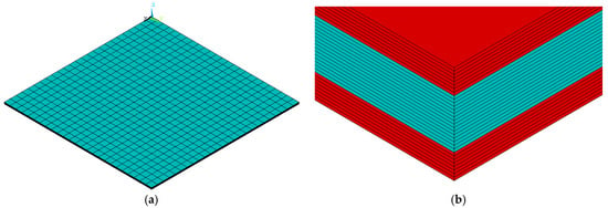
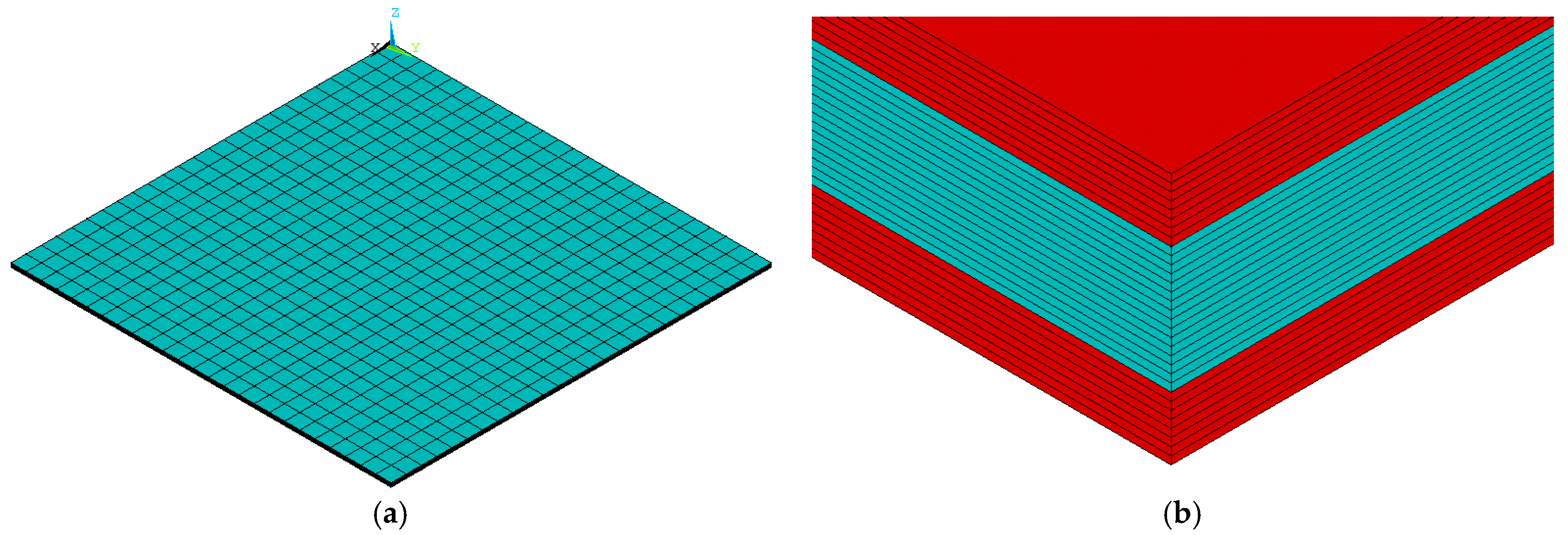
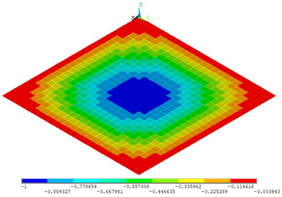
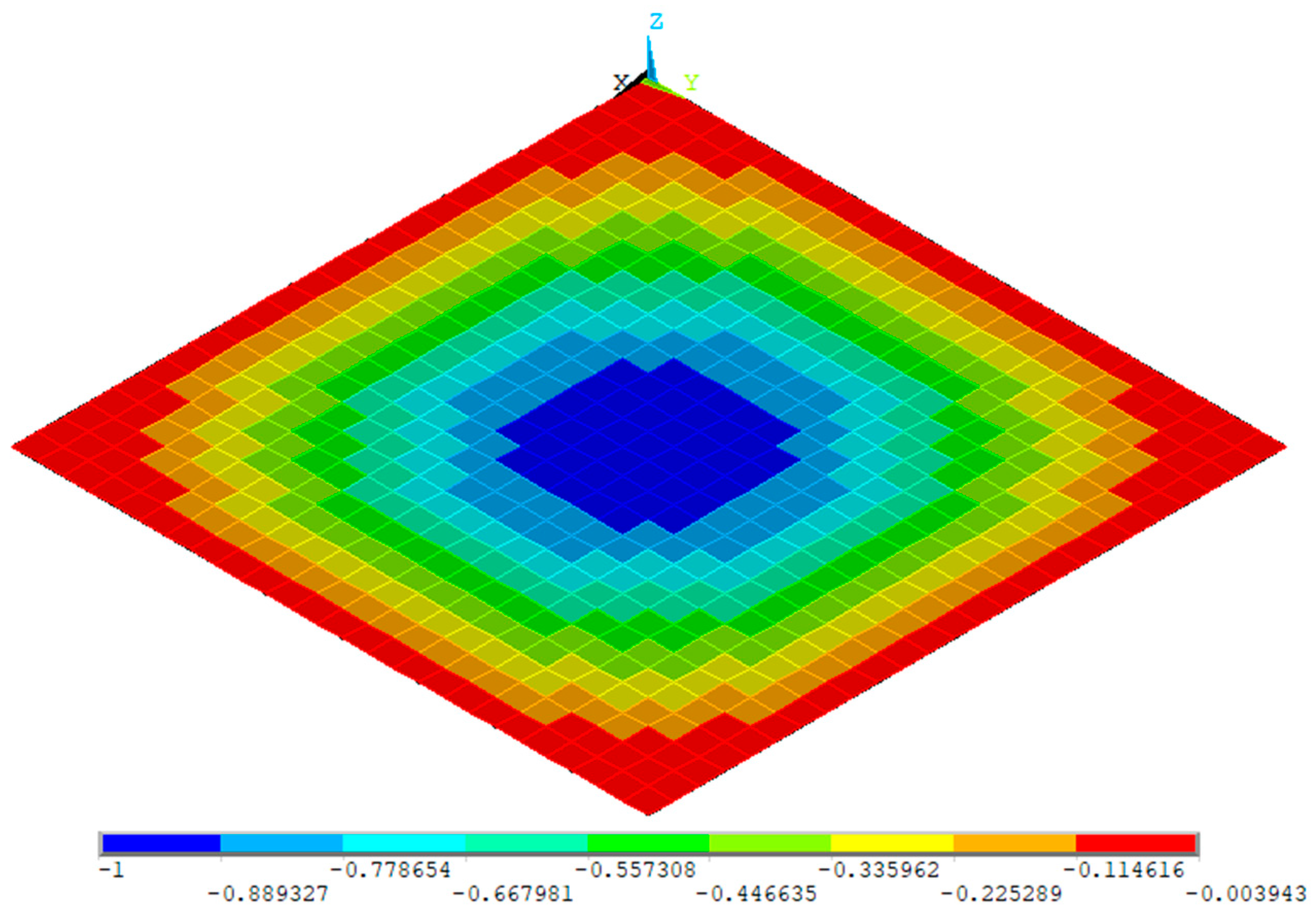
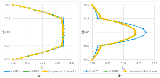
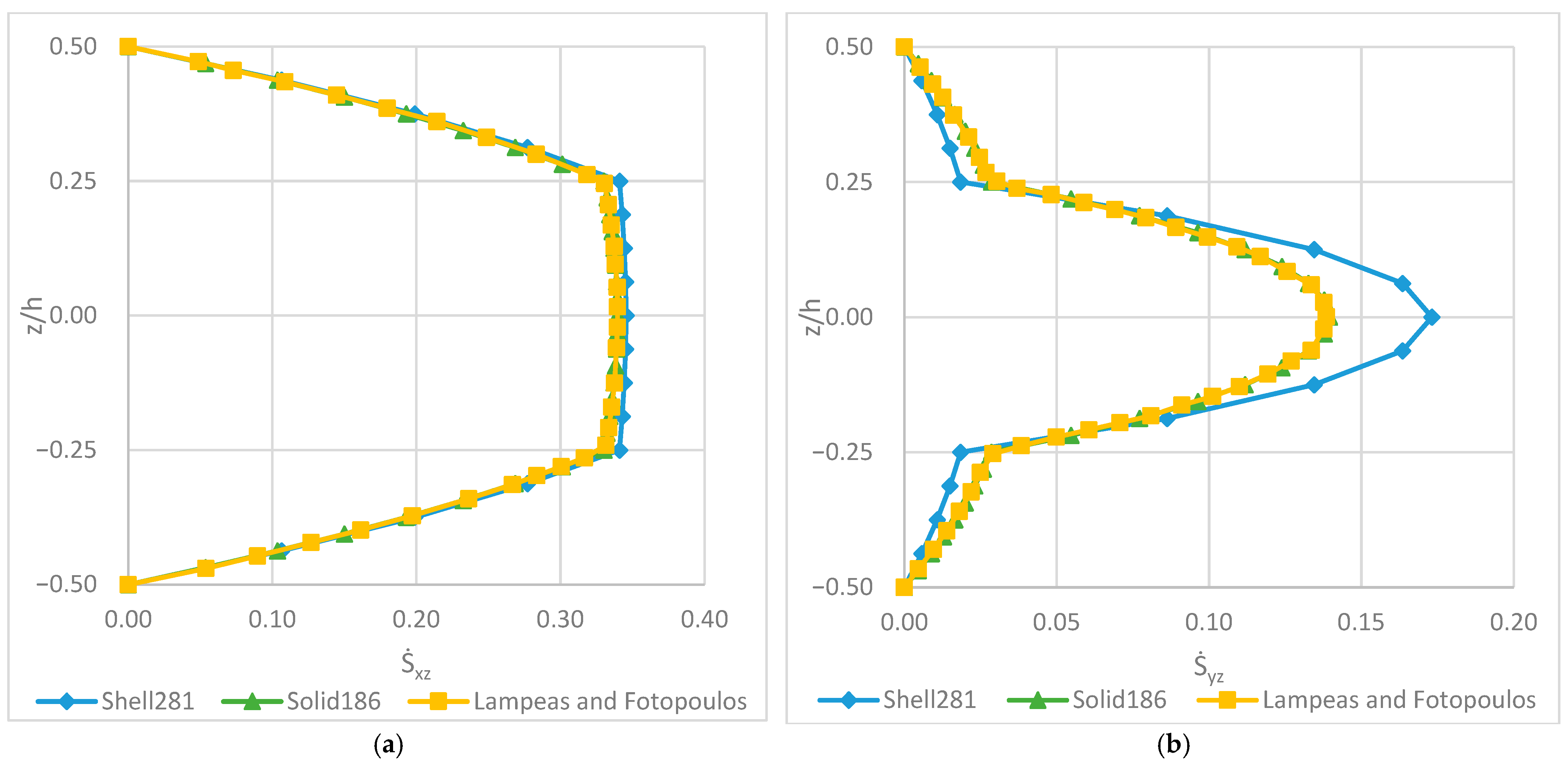
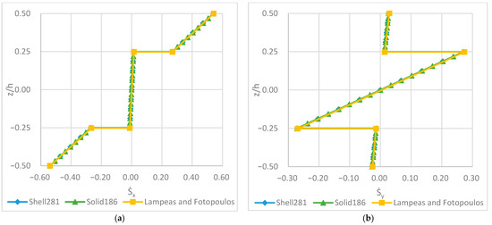
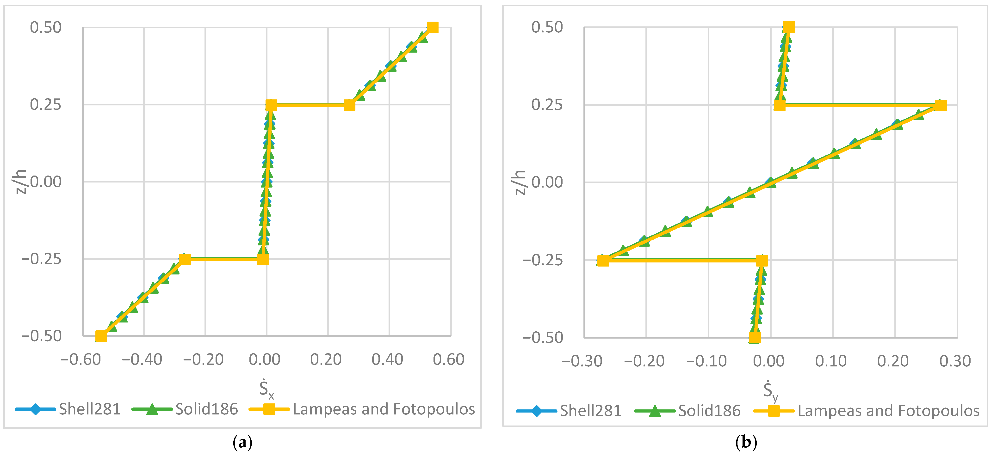
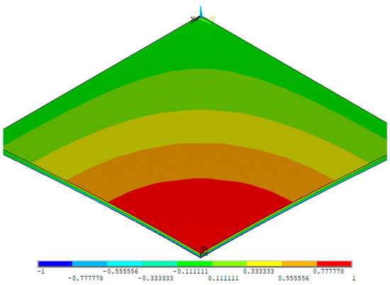
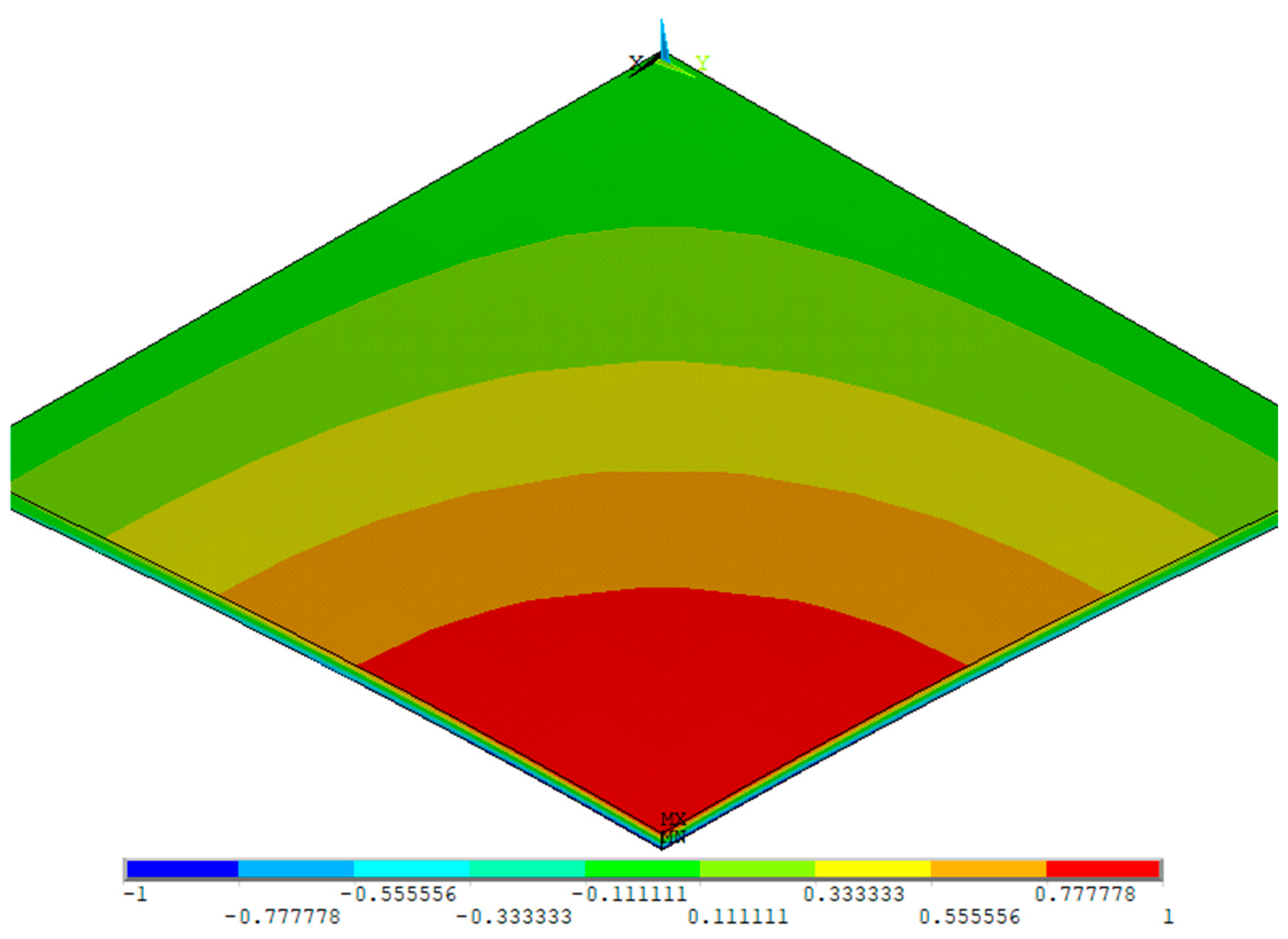
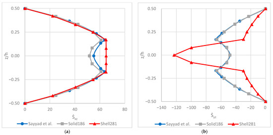
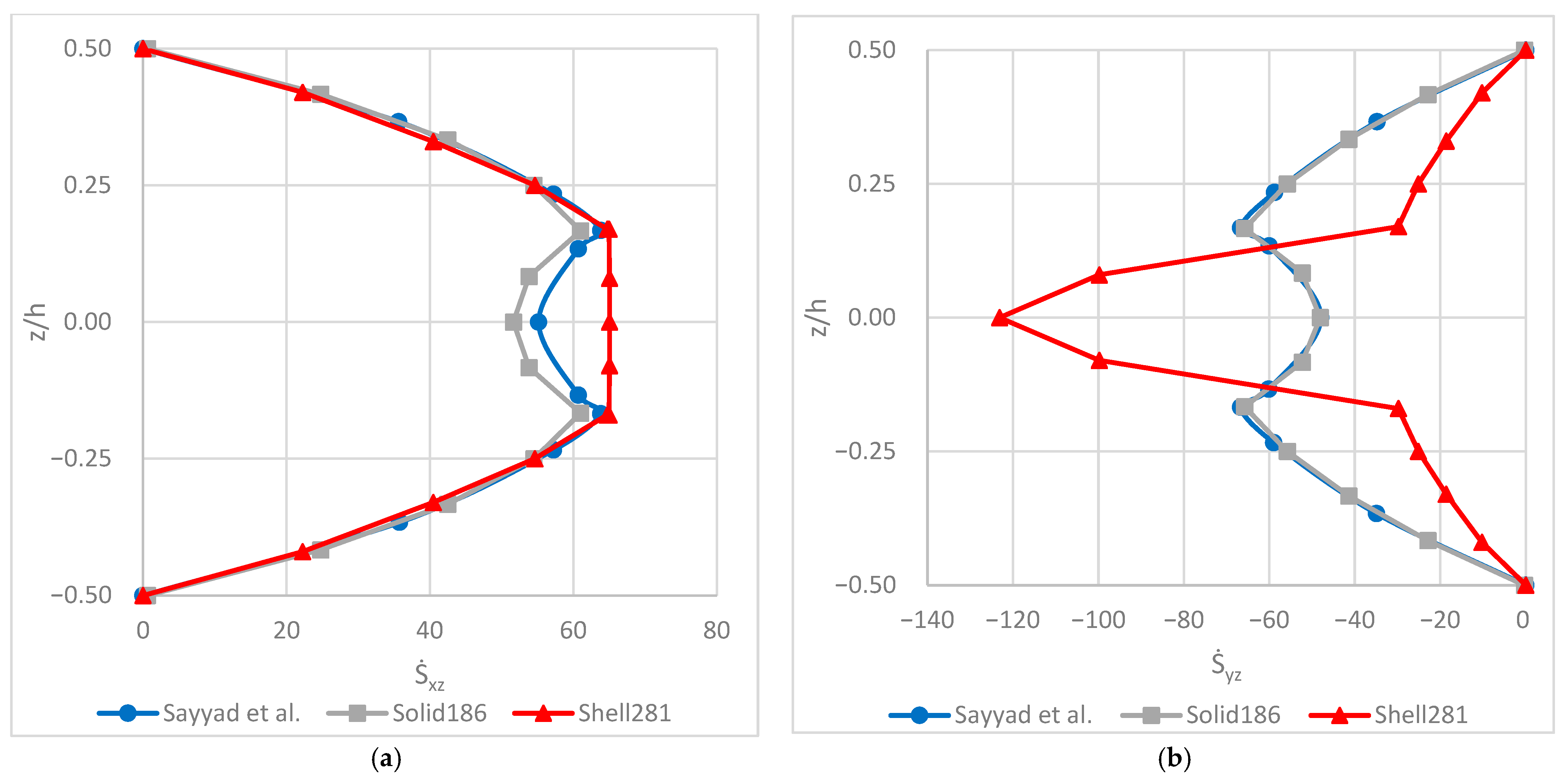
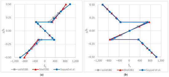
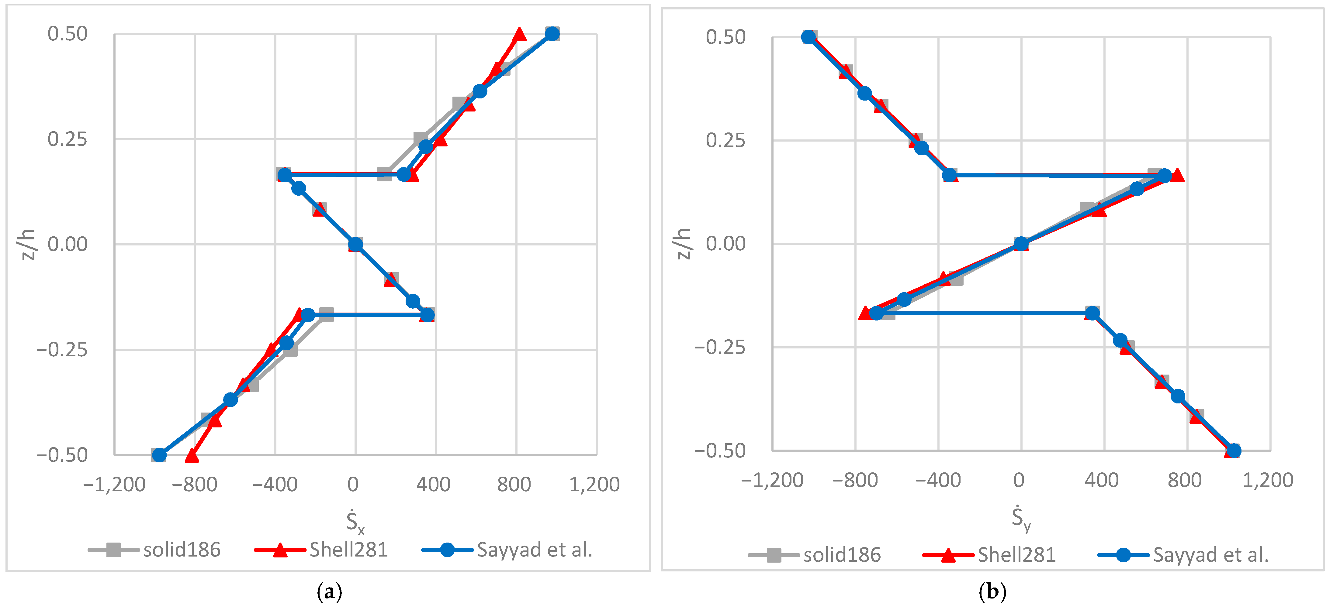
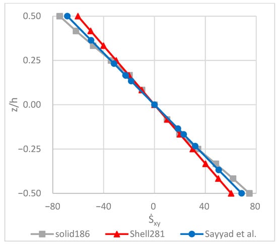
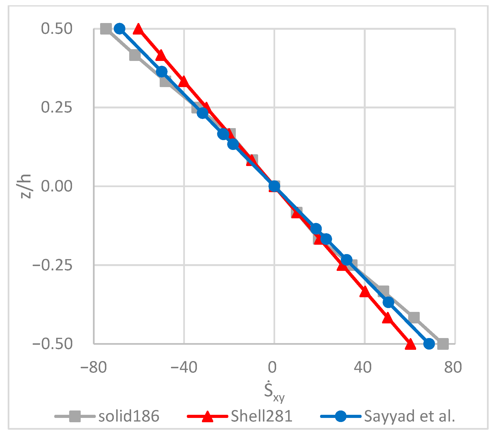
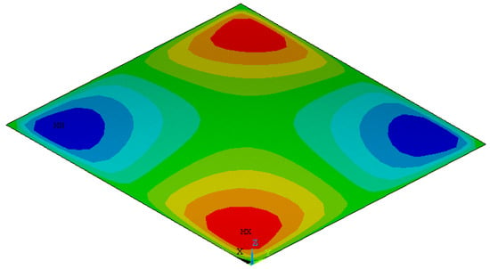
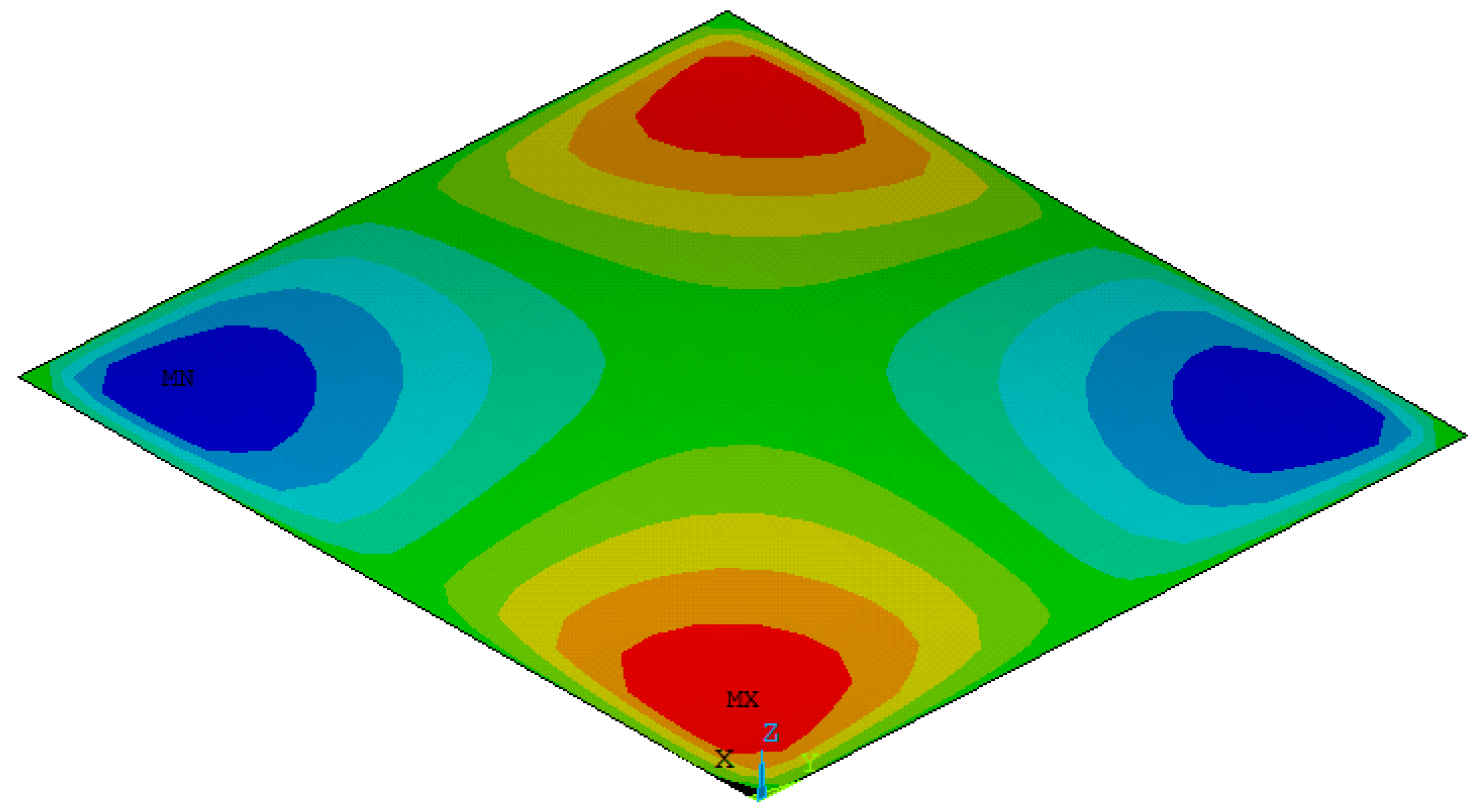
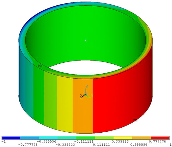
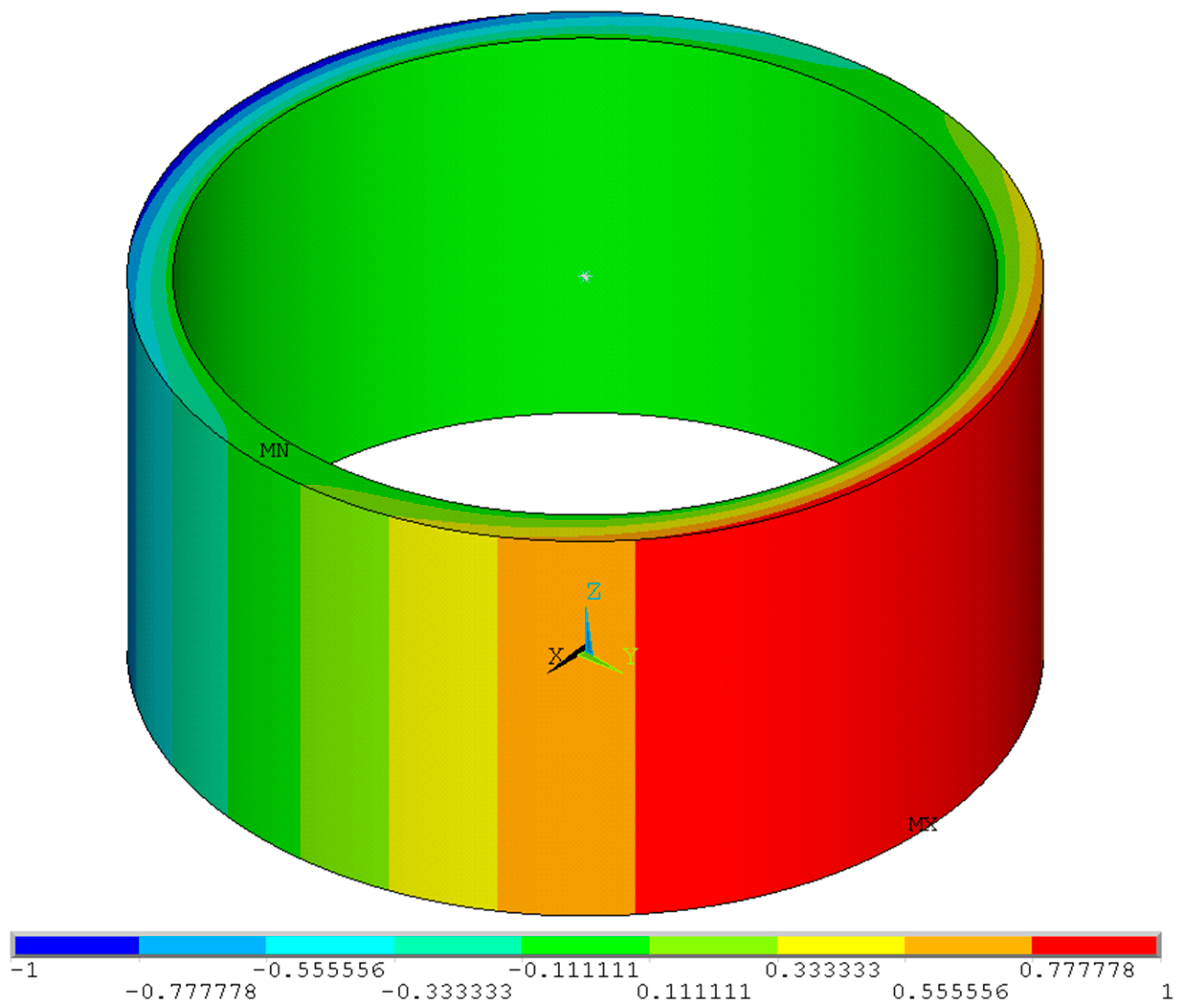
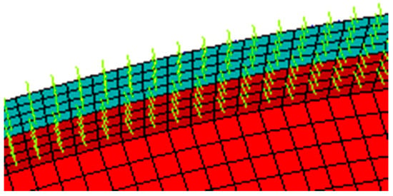
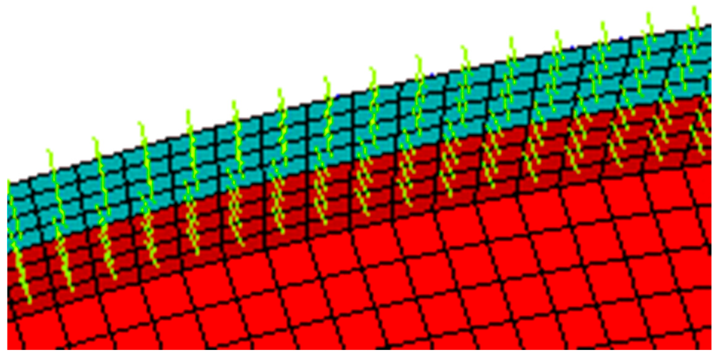
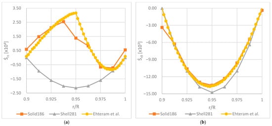
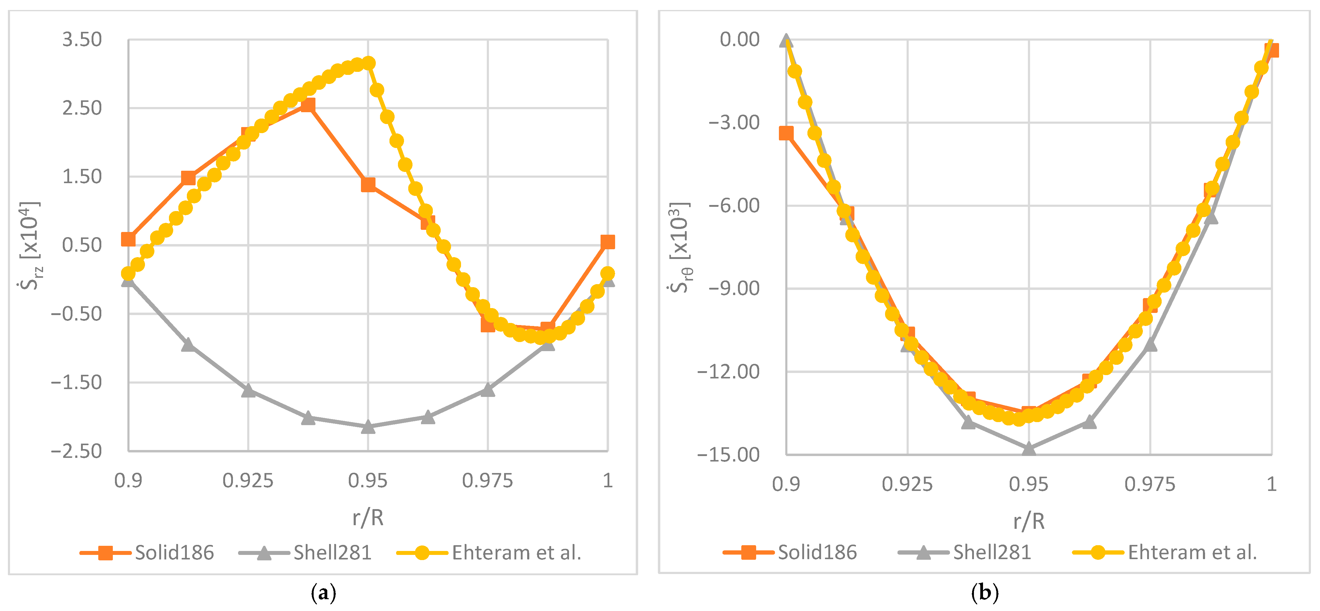
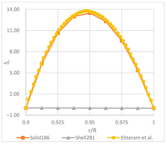
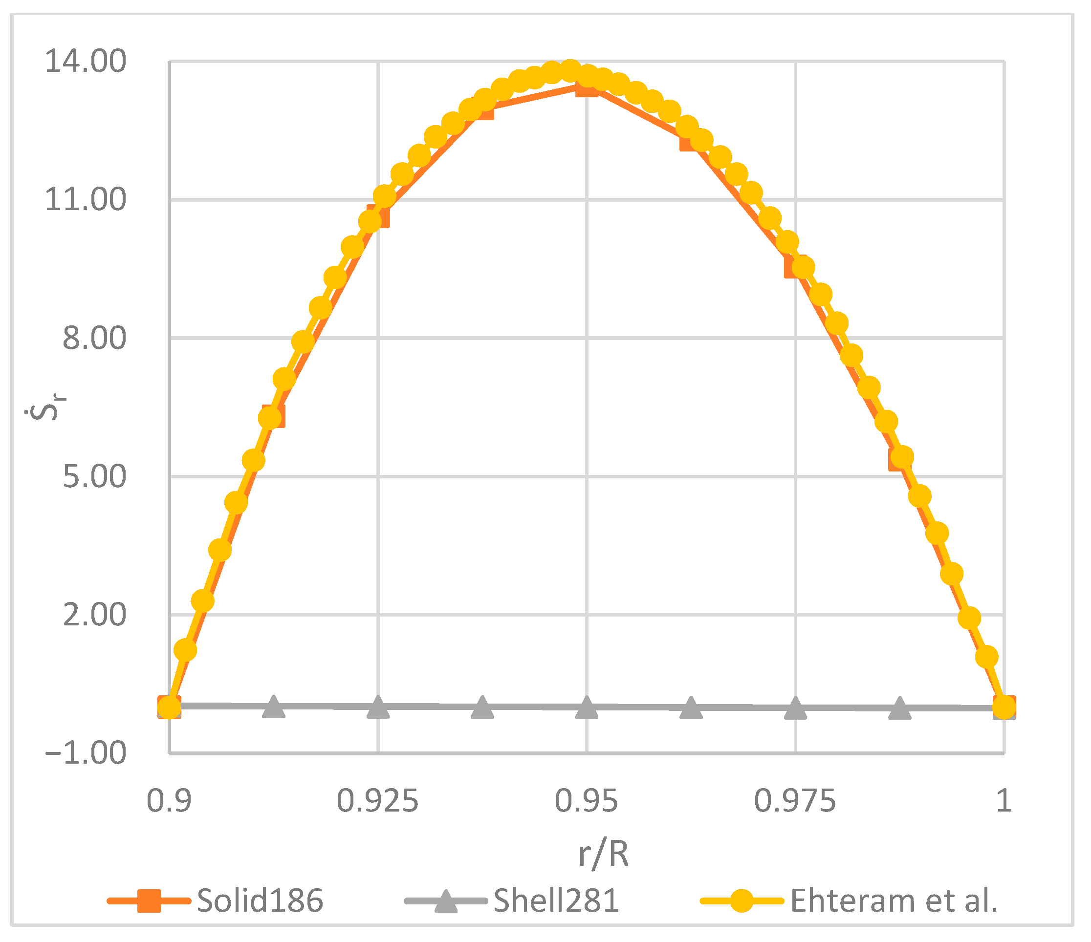
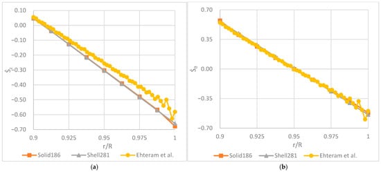
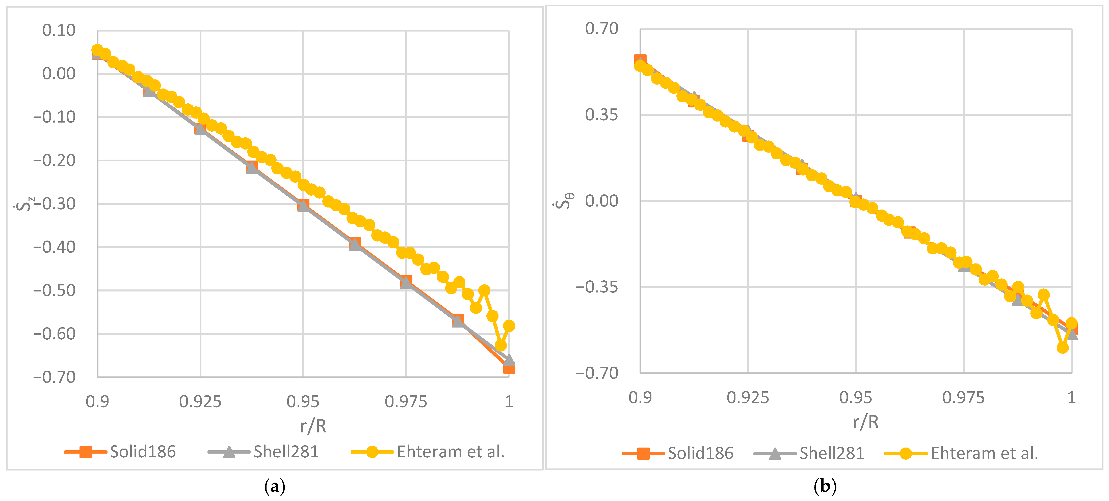
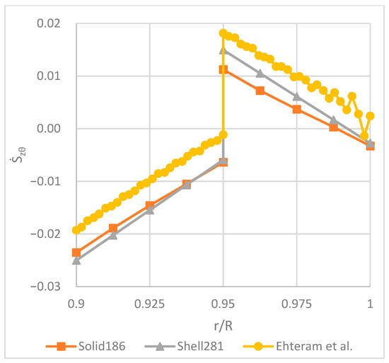
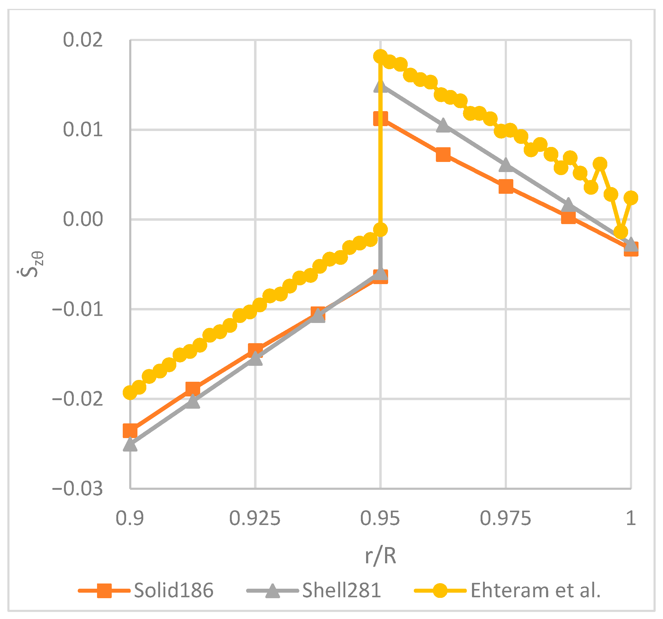
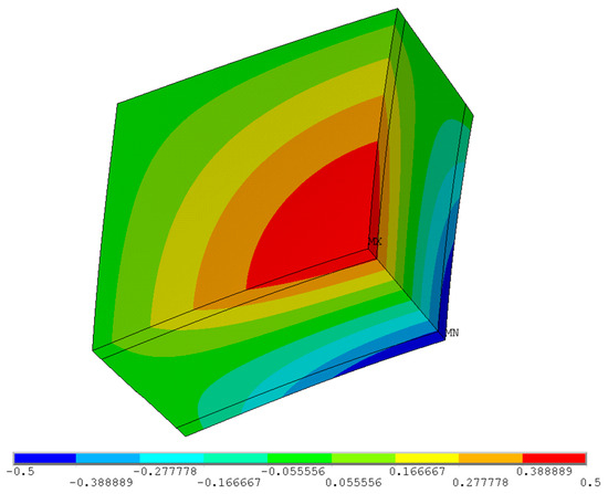
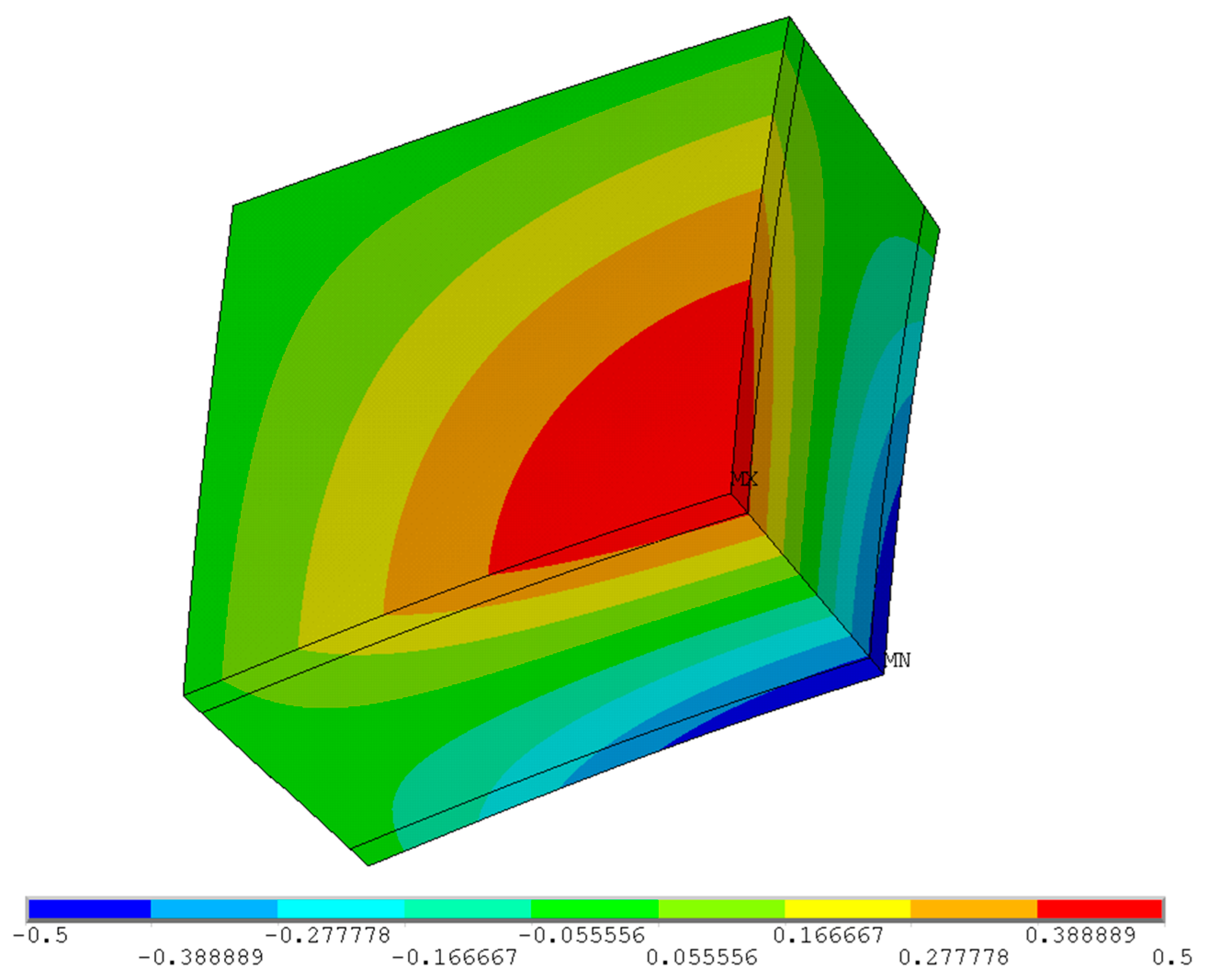
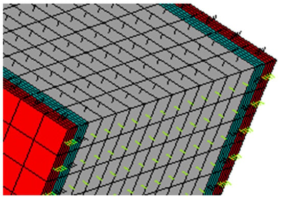
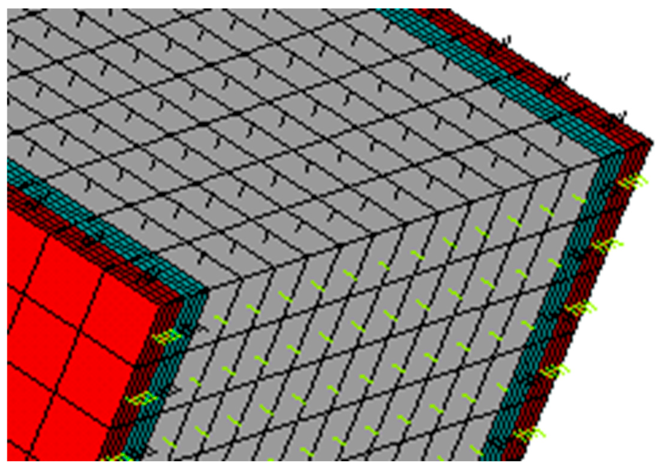
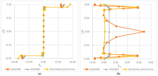
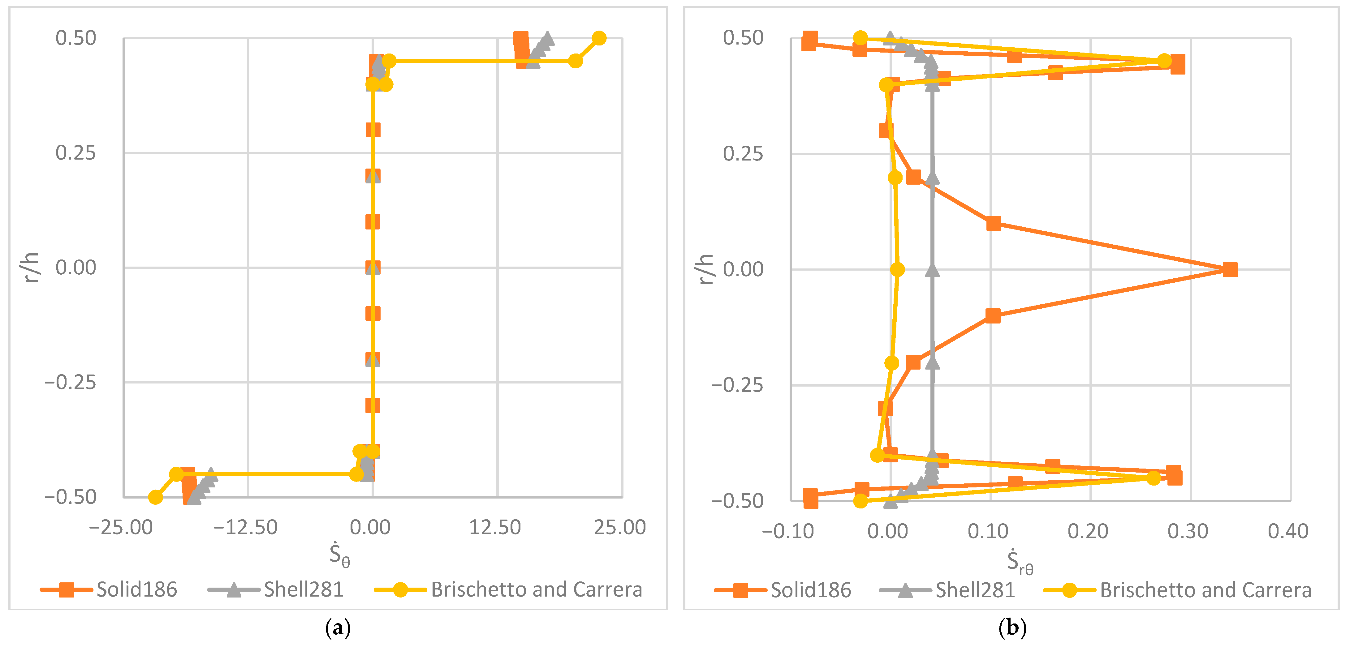
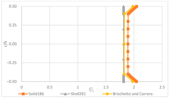
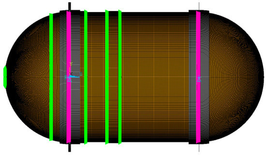
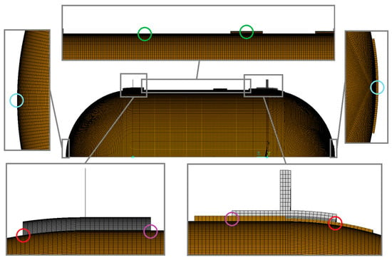
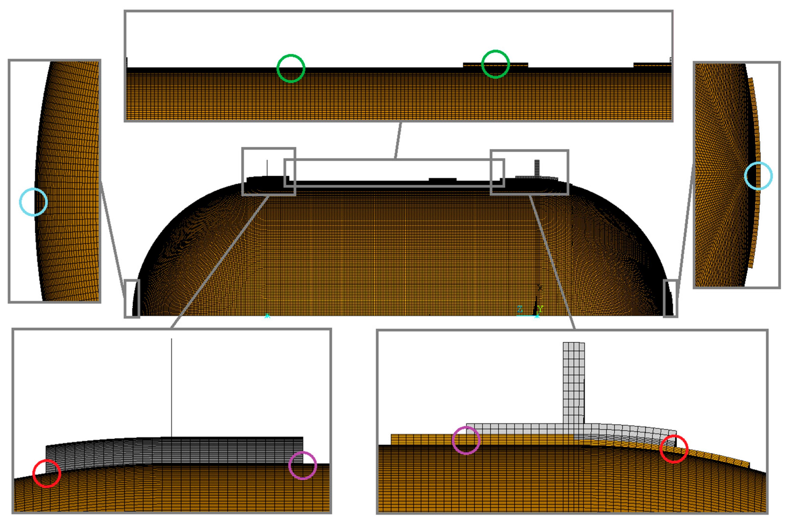
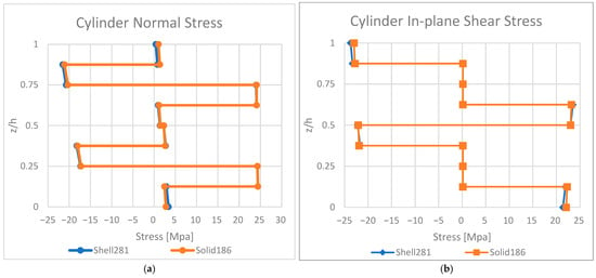
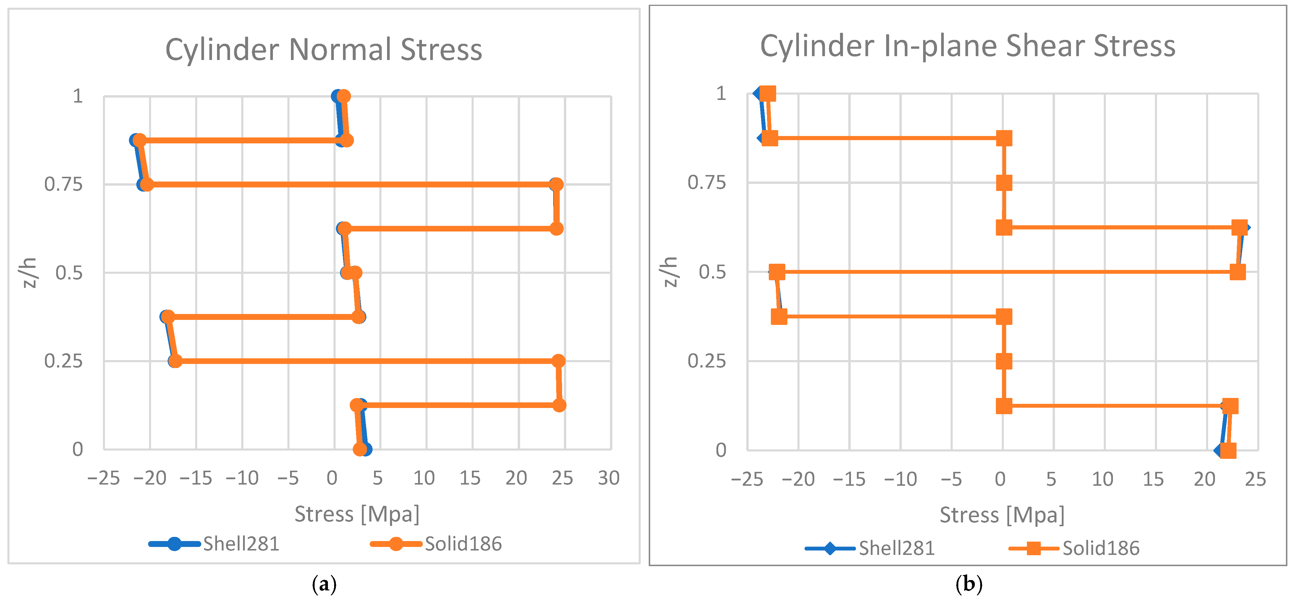
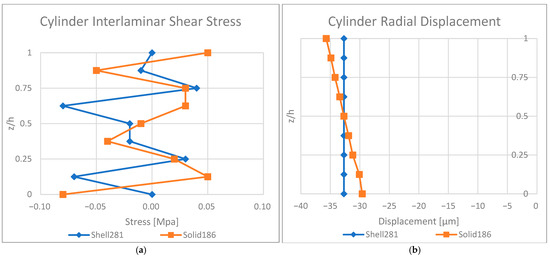
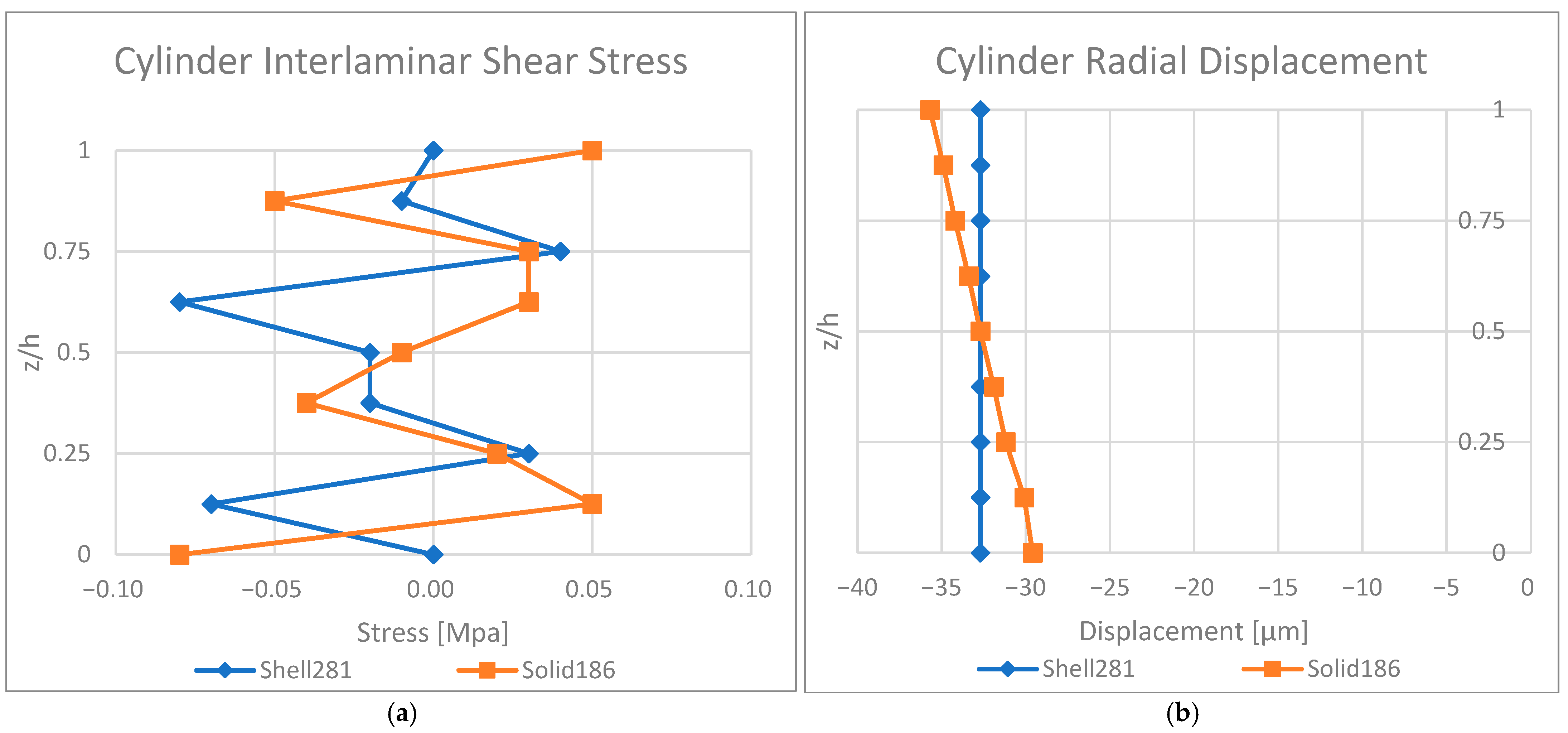
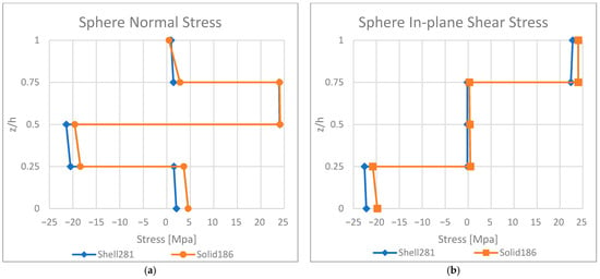
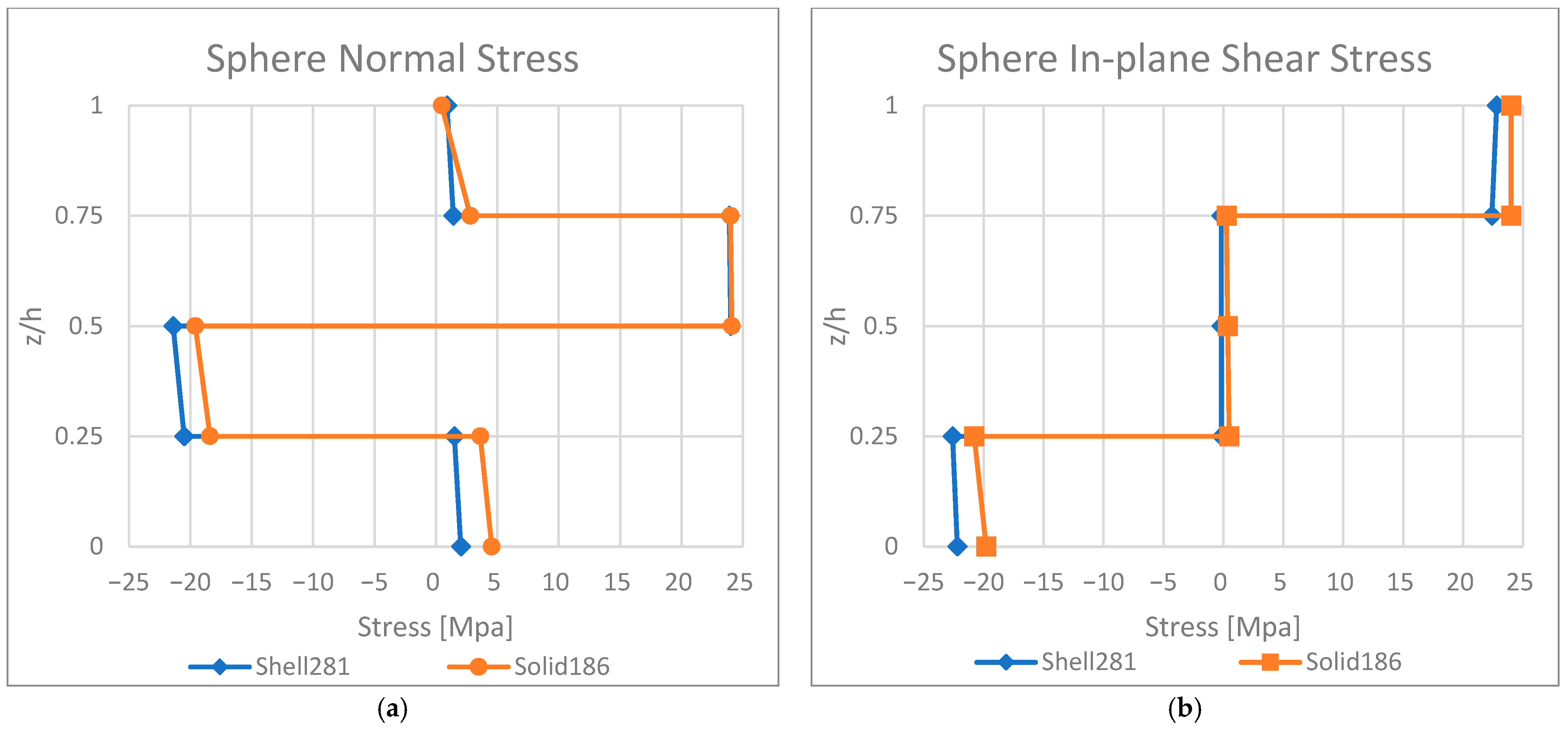
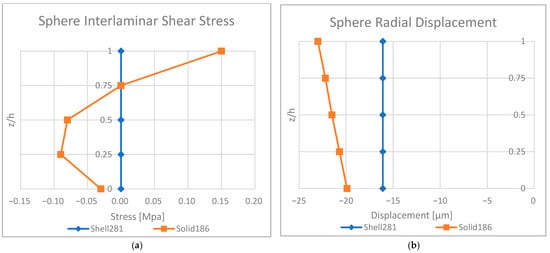
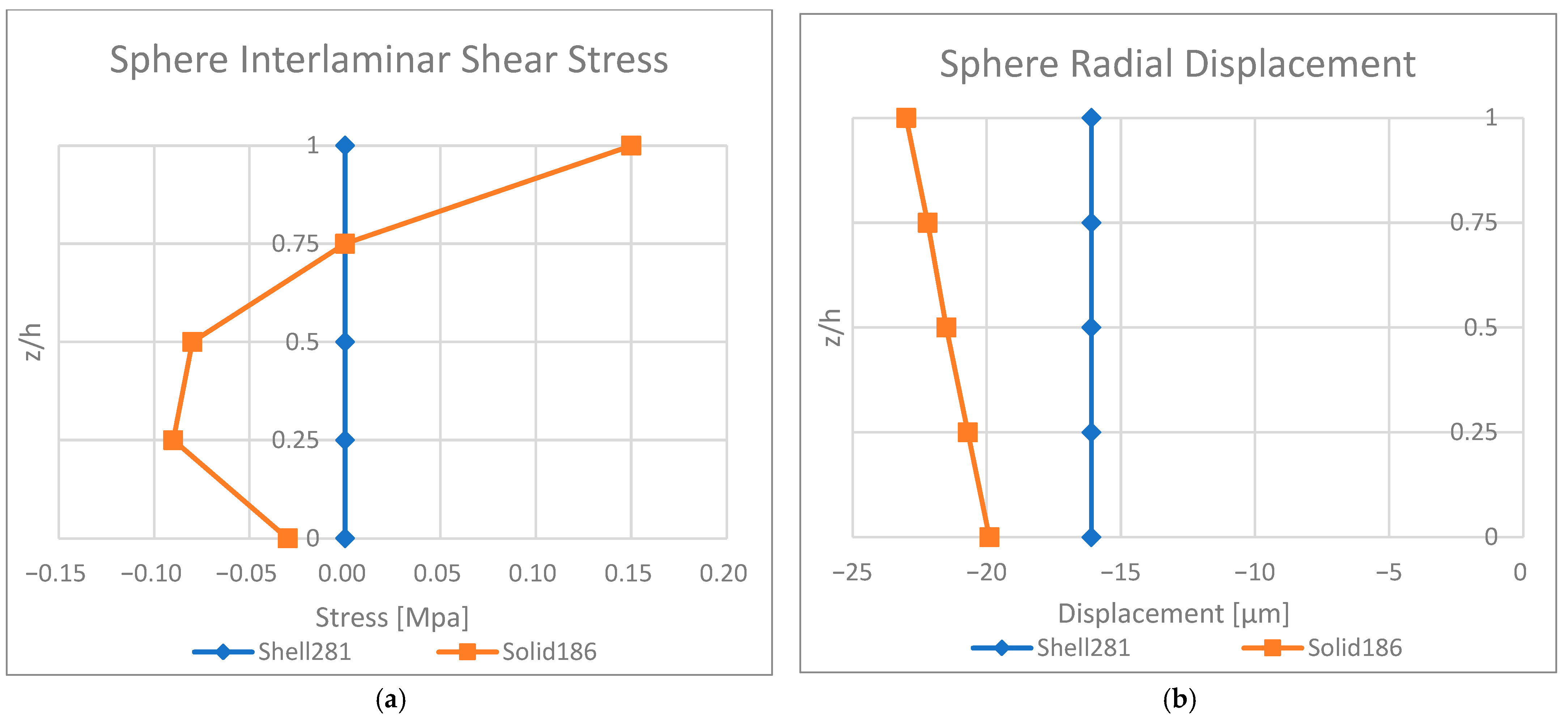
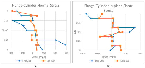
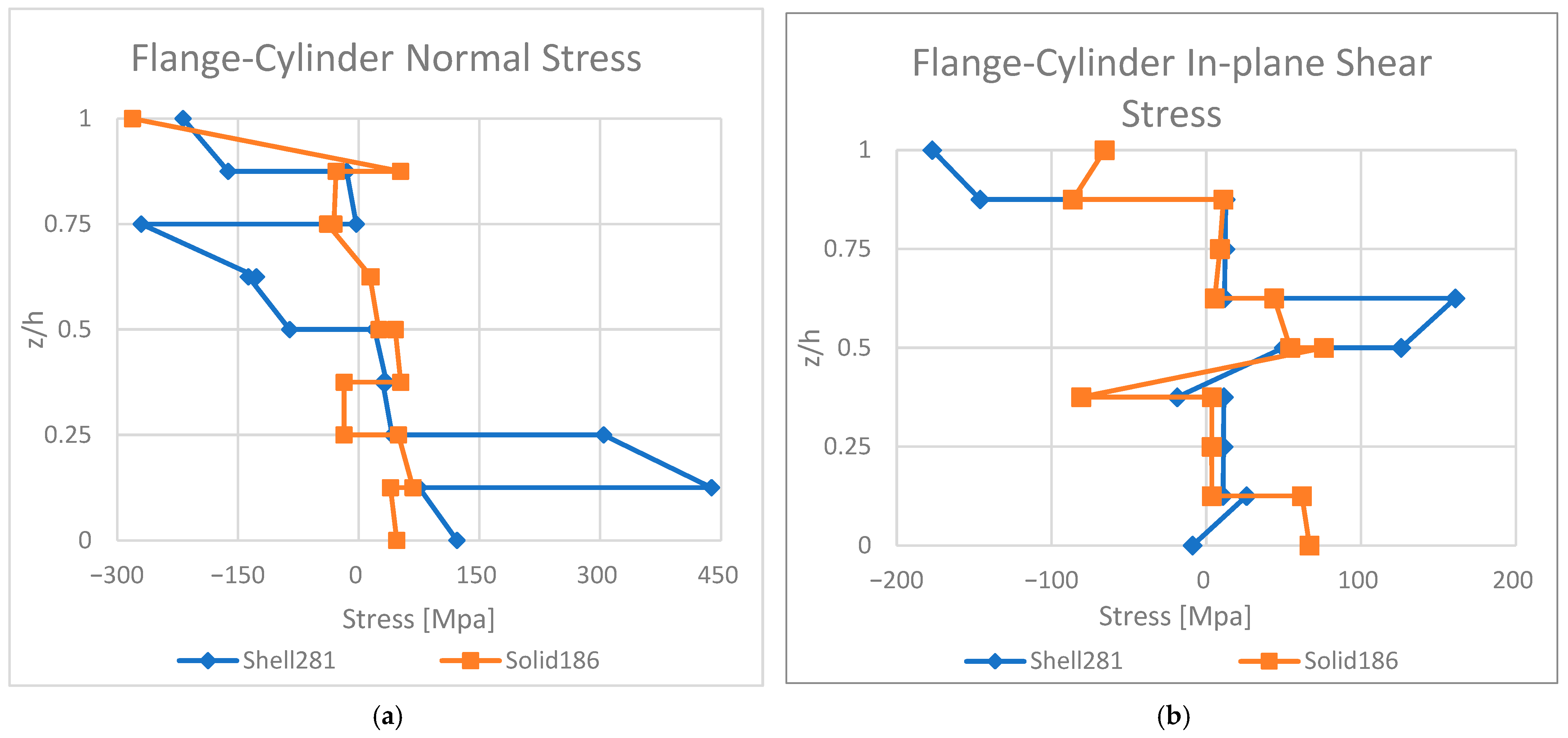
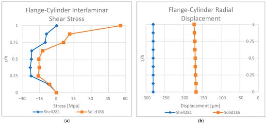
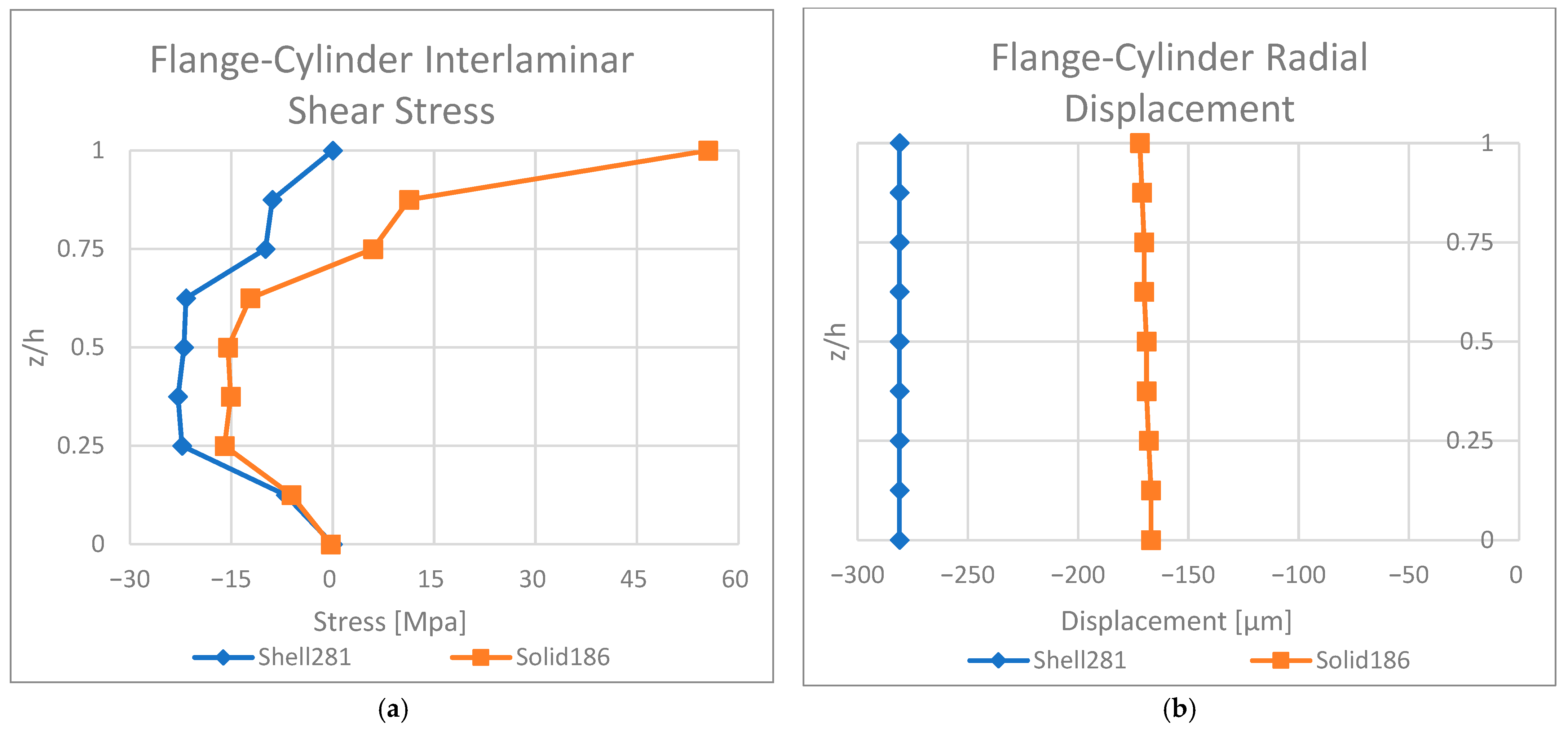
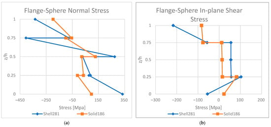
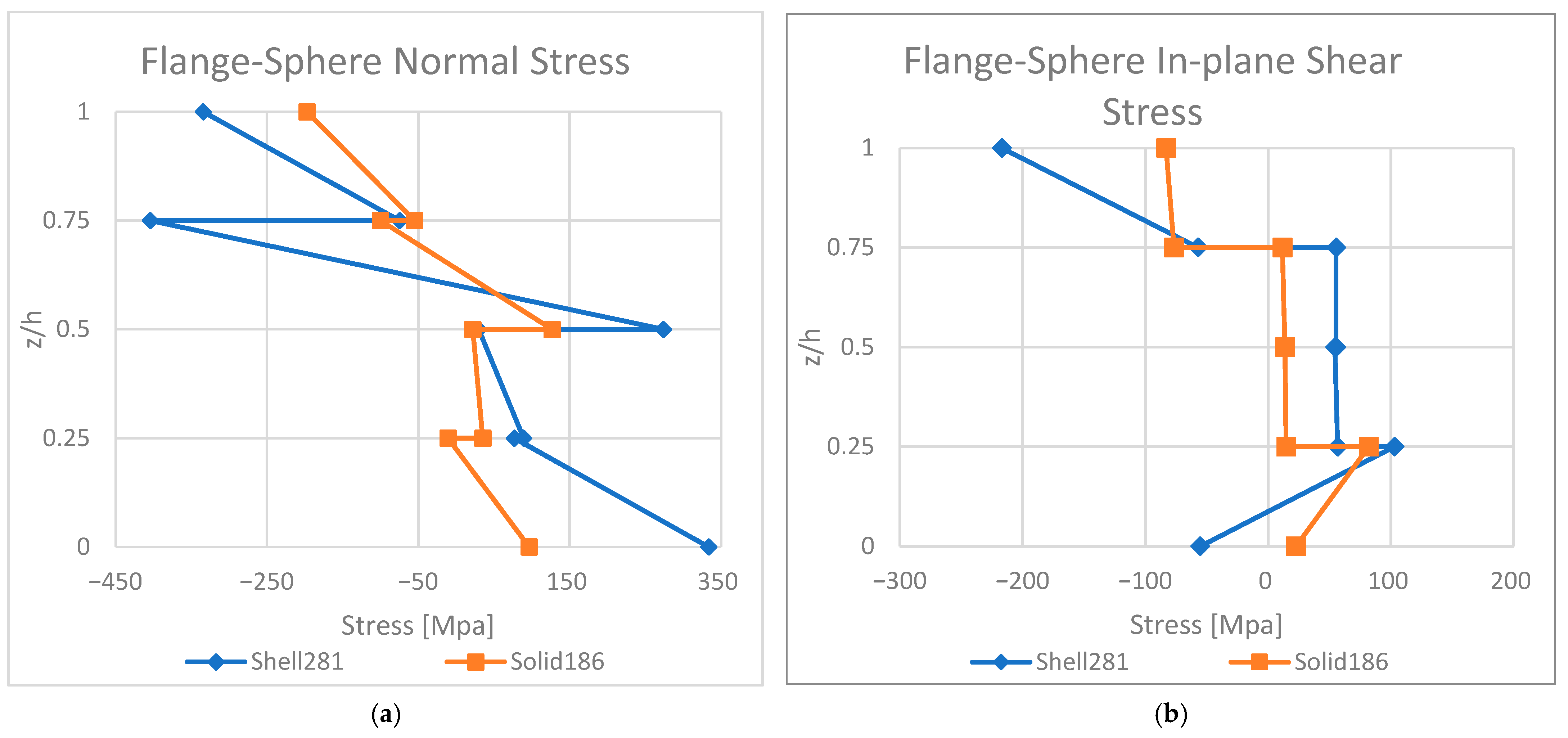
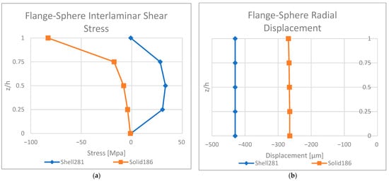
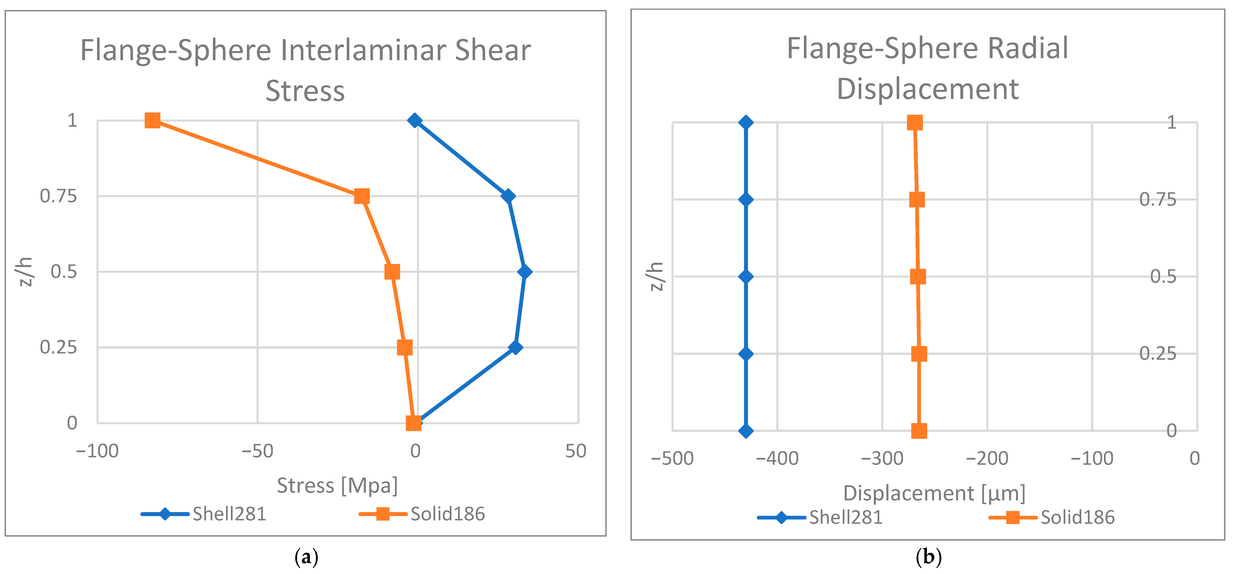
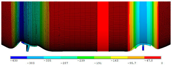
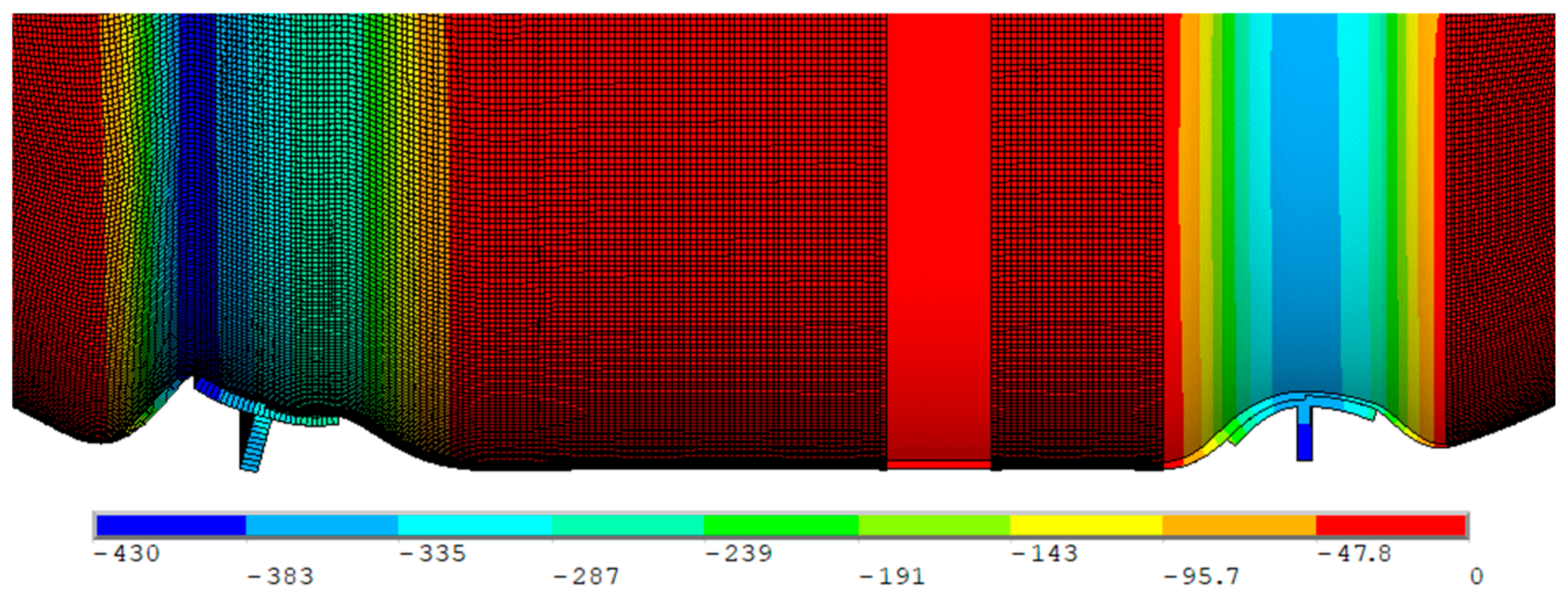
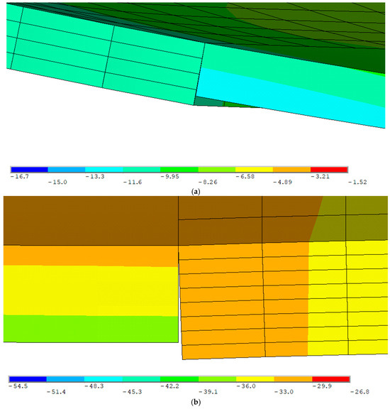
Disclaimer/Publisher’s Note: The statements, opinions and data contained in all publications are solely those of the individual author(s) and contributor(s) and not of MDPI and/or the editor(s). MDPI and/or the editor(s) disclaim responsibility for any injury to people or property resulting from any ideas, methods, instructions or products referred to in the content. |
© 2026 by the authors. Licensee MDPI, Basel, Switzerland. This article is an open access article distributed under the terms and conditions of the Creative Commons Attribution (CC BY) license.