


Abstract
The process of predicting mechanical properties in composite materials is an important challenge owing to their nonlinear and composition-dependent nature. In this research, a hybrid deep learning architecture fusing Artificial Neural Network (ANN) with Long Short-Term Memory (LSTM) networks is employed for the prediction of tensile strength, flexural strength, impact strength, and hardness for different weight composition composites. The composite was prepared with fiber contents of 0%, 5%, 10%, and 15% and was tested mechanically with respect to four different tests—tensile test, flexural test, impact test, and hardness test—to study the influence of fiber content variation on the physical characteristics of the material. The experimental dataset was used for both training and validation, while the intermediate compositions were suitably estimated using the devised hybrid architecture. It is observed that the ANN LSTM model exhibits superior predictability with R2 greater than 0.996 in all cases, which validates its capability to model complex material-property relations. This hybridization is a very computationally efficient and reliable approach for material optimization by minimizing the need for large-scale experimental trials. The results substantiate the value of ANN LSTM hybridization as a very strong predictive tool for composite material engineering.
1. Introduction
Composite materials have become indispensable in modern engineering due to their superior strength-to-weight ratio, durability, and adaptability compared to traditional conventional alloys and polymers [1]. Their applications span aerospace, automotive, civil infrastructure, and biomedical fields where mechanical performance, including tensile strength, flexural resistance, impact toughness, and hardness, is of paramount importance regarding reliability and service life [2]. Traditional experimental approaches have been very accurate for the characterization of these properties; however, they are resource-intensive, time-consuming, and limited in scalability [3]. This has motivated the adoption of machine learning and deep learning approaches for the prediction and optimization of properties, allowing for data-driven material design and accelerated discovery [4].
Artificial Neural Networks (ANN) have been widely used to model nonlinear correlations of composition and processing parameters with mechanical properties of composites [5]. As an example, ANN-based models successfully predicted the hardness and tensile strength in LM4 metal matrix composites [6] and tensile and flexural properties in wood–polymer systems [7]. The application of ANN frameworks was extended to hybrid polymer composites reinforced with hexagonal boron nitride (h-BN), giving accurate predictions of strength and toughness [8]. Similarly, ANN has also been deployed for cementitious composites incorporating fly ash and waste slag and demonstrated strong generalization across heterogeneous datasets [9].
Machine learning techniques are being used more frequently for predicting the mechanical behavior of composite materials and cementitious materials, from feedforward systems to more sophisticated systems that allow retention of knowledge as the behavior of material properties changes over time and process stages. The above-mentioned change is particularly applicable to those materials whose performance is dependent on time-sequence phenomena like the development of concrete strength in curing time or cumulative deformation of composite material during the manufacturing process. The LSTM network and its variants have been suggested for solving this class of problems based on the ability of the system to maintain knowledge through a series of inputs.
In the case of concrete, Prem Anand et al. [10] developed a lightweight Bi-LSTM model that predicted the mechanical properties but did so with great accuracy while maintaining a computational efficiency of the network sufficient for practical implementation despite the validation being limited to only a small range of mix types. With respect to composite materials, Deng et al. [11] utilized the CNN-LSTM framework in combination with finite element analysis in order to estimate the spatio-temporal, curing-related deformations of composite structures and found that the combination of spatial feature extraction and sequential learning led to better prediction of deformations; nevertheless, since the authors used the FE-based data for training, the issue of transferability of the proposed model to experimentally measured deformations remains open. Jian et al. [12] used a bidirectional LSTM network to forecast very high-cycle fatigue behavior of thin plates made of CFRP subjected to random loadings, showing that a recurrent model is able to take advantage of the sequence in fatigue data better than the traditional regression approach, but only one laminate sample was used for reporting the performance of the model.
One challenge that can be found in most of these LSTM models is the lack of sufficient experimental data for training due to the fact that labeled data is hard to obtain. Cheung, Uvdal, and Mirkhalaf [13] tackled the problem directly by suggesting methods of augmenting the data used to train deep learning models for composites, leading to significant improvements in the robustness of models trained on small amounts of experimental data. Though this approach provides a clear way forward for making recurrent and hybrid models stronger, it also clearly demonstrates that data shortage is an unresolved issue.
In addition to sequential models, standard ANN models as well as hybrid ANN models were also applied for the prediction of material behavior using static or geometrical parameters. Maheswaran et al. [14] employed an implicit geometric descriptors-based ANN to forecast the properties of architected nanofibrous material such as Young’s modulus, maximum stress, and energy absorption. This approach is accurate but is highly dependent on the exact geometric representation that might not be available for fabricated materials. Wang et al. [15] used FEM with ANN to predict the flexural strength of CFRP-reinforced concrete T-beams, and Zhao et al. [16] used ANN models for estimating tensile and compressive strengths for recycled mortar systems; however, both these studies reveal that ANNs could be used as an alternative to expensive experiments or simulations, but the samples used in both cases were relatively smaller than other reviews, e.g., Qiu and Yang [17], that conclusively reinforce this trend in the field, suggesting that model-based approaches are increasingly becoming an essential part of composite design. However, most models described have been validated through independent data sets, without standardized comparison among them. Ulkir and Ersoy [18] combined ML with experimental testing for characterizing polymer composites formed by the FDM method and demonstrated the superior performance of ANN compared to regression techniques for the identification of nonlinear and multivariate relationships, whereas Sharma et al. [19] applied ML for predicting hardness in polypropylene/carbon nanotubes and LDPE/carbon nanotube composites.
Despite this progress, the integration of ANNs with sequential learning methods such as LSTM remains underexplored in composite material studies. A majority of prior works are limited to either static ANN frameworks or purely temporal LSTM models without full exploitation of their respective complementary strengths.
The present study fills this gap in the literature by proposing a hybrid ANN–LSTM technique in order to model the tensile, flexural, impact, and hardness properties of composite materials. By capturing both nonlinear correlations and sequential dependencies, the proposed approach ensures consistently high prediction accuracy with performance metrics such as R2 exceeding 0.996, hence demonstrating strong applicability for intelligent material design in Industry 4.0 frameworks.
It is important to clarify why an LSTM component is included despite the discrete nature of the composition levels (0%, 5%, 10%, and 15%) rather than a continuous time series. Here, the LSTM does not model physical time; instead, the four composition levels are treated as an ordered sequence, and the LSTM gating mechanisms are used to learn the monotonic trend and rate-of-change relationships between successive filler-loading steps information that a purely feed-forward ANN would treat as independent, unordered inputs. This sequence-aware treatment is intended to yield smoother and more physically consistent interpolation at untested intermediate compositions than a feed-forward-only model, at the cost of added architectural complexity. We acknowledge that this benefit has not yet been directly benchmarked against a feed-forward-only ANN baseline on this dataset, and we identify this comparison as an important direction for future validation of the hybrid architecture.
2. Materials and Methods
2.1. Materials Selection and Preparation
The composite specimens examined in the present research work were fabricated using thermosetting polyester resin as the main matrix material. This resin system was chosen because of its favorable properties, such as good mechanical performance, dimensional stability with variable environmental exposure, and suitability for easy processing by conventional manufacturing techniques. Polyester resin belongs to the epoxide family, possessing excellent compatibility with both natural and synthetic reinforcement materials at a reasonable cost regarding structural composite applications.
Sisal fiber and cashew nut shell agricultural waste biochar-based fillers are incorporated into the matrix system. These reinforcement materials were chosen based on a number of considerations, including their wide availability as wastes, environmental sustainability, biodegradability, and proven potential to improve both mechanical load-carrying ability and erosion resistance characteristics of polymer composite systems.
All the filler materials were subjected to various systematic preparation procedures prior to their incorporation into the matrix to ensure their best performance in the final composite. The raw filler materials were subjected to thermal drying processes with the intention of removing the residual moisture content to avoid interference with resin-filler bonding. The dried materials were then mechanically milled using high-speed grinding equipment to reduce their particle dimensions. The milled particles were passed through standardized sieves for uniformity of particle size distribution within a controlled range, ensuring homogenous dispersion throughout the resin matrix and promoting consistent mechanical properties among all fabricated specimens.
2.2. Composition Formulations
Four different filler loading configurations were established for this investigation, representing systematically varied reinforcement levels, as presented in Table 1. These specific loading fractions were deliberately selected to facilitate exhaustive characterization of how progressive filler content influences mechanical behavior for the resultant composite materials. The baseline composition, without any filler content, represents the control formulation and offers reference values of mechanical properties for the neat polyester matrix. The intermediate loading levels allow the systematic study of property improvement mechanisms with increasing filler content. Also, these discrete experimental compositions offer the necessary data structure for the development of predictive computational models, which can estimate the mechanical properties at untested, intermediate filler fractions throughout the investigated range of composition.
Table 1.
Composite formulations with varying filler loadings used in this study.
2.3. Specimen Fabrication Procedure
The process of preparing the composite specimen is shown in Figure 1. The composite specimen was prepared by a combination of hand lay-up and compression molding, which is one of the methods used to produce polymer composite materials that ensures consistent quality and dimensional accuracy. For each composition formulation, measured quantities of polyester resin and filler materials were determined with the use of calibrated digital weighing equipment for the purpose of attaining proper weight percentages. The weighed resin and filler components were mixed together in a mixing vessel and subjected to vigorous mechanical stirring with the aim of homogeneously distributing the filler particles in the liquid resin. Particular attention was paid to the breaking up of any agglomerates that may have formed and to ensuring that the filler surfaces were fully wetted by the resin matrix. After proper mixing, a proper amount of curing agent, namely methyl ethyl ketone peroxide, was added together with an adequate accelerator compound, which provided the proper initiation of cross-linking polymerization reactions. The catalyzed mixture of resin and filler was carefully poured into pre-prepared molds with cavity dimensions according to the needs of subsequent mechanical testing standards. The compression pressure in filled molds was controlled at ambient temperature. The objectives of this compression include eliminating entrapped air bubbles, which may create void defects, ensuring uniform thickness throughout the specimen, and developing intimate contact between the resin and the filler surfaces.
Figure 1.
Composite specimen fabrication steps.
Demolded composite laminates were then given post-curing heat treatment after initial ambient temperature curing for a specific duration, during which the main cross-linking reactions could proceed substantially to completion. Such an elevated temperature increases the degree of polymerization and the density of cross-links in the polymer network, hence improving the mechanical strength and dimensional stability of the final composite specimens. The post-cured laminates were subsequently machined into the final test specimen dimensions based on the geometry requirements of the respective testing standards.
2.4. Methodology Overview
Figure 2 presents the proposed framework for the hybrid ANN-LSTM methodology in predicting mechanical properties of biochar-reinforced polyester composite materials.
Figure 2.
Hybrid ANN-LSTM methodology.
The research framework sets the structure for the deep learning architecture that merges artificial neural networks with long short-term memory networks. Mechanical property data is collected through experimental processes of mechanical testing at discrete filler loading levels (0%, 5%, 10%, 15% by weight) with five replicate specimens for every composition, while tensile strength was assessed using ASTM D3039/D3039M [20,21], flexural strength was measured according to ASTM D7264/D7264M [20,22], impact strength tested via ASTM D256/D256M [20,23] and hardness according to ASTM E384/11e1standard [24,25] Data preprocessing involves normalization, feature scaling, and the train–test split to create optimal conditions for the model to be trained. The hybrid architecture will merge the ANN layers for feature extraction with the LSTM layers for sequential modeling, optimized with the mean squared error loss function and using the Adam and RMSprop optimizers with tunable hyperparameters: learning rate, batch size, epochs, and hidden units. Model performance will be evaluated using five statistical metrics, namely, mean absolute error, mean squared error, root mean squared error, mean absolute percentage error, and coefficient of determination, to affirm its prediction accuracy and generalization capability.
2.5. Research Framework
The present study is based on a hybrid deep learning architecture that combines ANN with LSTM networks to model the mechanical properties of biochar-reinforced polyester composites for different filler composition percentages. The methodological scope includes experimental data collection, rigorous preprocessing procedures, hybrid model architectural design, protocols for training and validation, and performance evaluation.
2.6. Mechanical Property Testing and Experimental Data Collection
Experimental measurements were acquired on composite test specimens fabricated at discrete intervals of filler loading: 0%, 5%, 10%, and 15% by weight, respectively, according to standardized testing protocols. Four critical mechanical properties were systematically measured.
Tensile Strength Evaluation: Tensile testing was done using a make/model universal testing machine, which was equipped with pneumatic grips, following the standards of ASTM D3039/D3039M. Tensile strength characterization was conducted following the standardized procedures outlined, which detail specimen geometry, requirements for apparatus, and procedural protocols for determining tensile properties of polymer materials. The dimensions of the rectangular specimens that were prepared from the cured composite laminates using precision cutting equipment included gauge length, width, and thickness. All tests were conducted on a universal testing machine using pneumatic or mechanical grips that provided uniform axial loading with no stress concentrations at the grip interfaces. The specimens were installed in the testing machine with careful attention given to alignment in order to ensure axial loading without bending moments. Tensile load was uniformly applied through a cross head displacement rate in accordance with the standard until specimen failure. The load applied and the resulting elongation of the specimen were measured continuously during the test. Tensile strength values were calculated from the load-displacement data as the maximum sustained load divided by the original cross-sectional area of the gauge section. In order to ensure statistical reliability in the measurement of tensile strength values, several replicate specimens of each composition were tested.
Flexural Strength Assessment: The flexural properties were determined in accordance with the ASTM D7264/D7264M standard test methods for flexural properties of unreinforced and reinforced plastics/polymers and electrical insulating materials. A three-point bending configuration is involved in this testing procedure, in which a simply supported beam specimen is loaded at its midpoint. Rectangular bar specimens with length-to-thickness ratios meeting the requirements of the standard were prepared from each composite formulation. The specimens were positioned on support spans separated by a certain distance; a loading nose with a prescribed radius was brought into contact with the specimen’s upper surface at the midpoint between supports. The tests were performed under a constant rate of cross-head motion, applying bending stress that varies linearly through the specimen thickness, with maximum tensile stress at the bottom surface and maximum compressive stress at the top surface. The applied load and corresponding center deflection were continuously recorded until specimen failure. Flexural strength was determined from the maximum load using standard beam bending equations, which took into consideration specimen geometry and support span configuration. Testing of several replicate specimens provided statistical validation of the measured flexural strength values.
Impact Strength Determination: Impact resistance was quantified using Izod impact testing methodology according to ASTM D256/D256M. This test method measures the energy absorbed by a specimen when fractured under high-rate loading conditions representative of sudden impact scenarios encountered in service applications. From the composite materials, notched specimens of standardized dimensions and notch geometry were prepared. The presence of a controlled notch introduces a stress concentration that ensures consistent fracture initiation location and promotes complete specimen fracture. Each specimen was mounted in a cantilever configuration, clamped at one end with the notch positioned on the tension side facing the direction of pendulum impact. Testing was done using a pendulum impact tester, previously calibrated and with known potential energy. The pendulum was then released from a standardized height, swinging through an arc to strike the free end of the cantilevered specimen opposite the clamped end. The energy absorbed during specimen fracture was determined from the difference between the pendulum’s initial potential energy and its residual energy after breaking the specimen, measured by the pendulum’s swing height on the opposite side. The impact strength was calculated as the absorbed energy divided by the cross-sectional area of the specimen at the notch location. Several specimens of each composition were tested to provide reliable average impact strength values along with statistical measures of variability.
Hardness Measurement: Surface hardness was determined through the Vickers hardness testing technique based on the ASTM E384/11e1 standard for micro indentation hardness of materials. The technique involves indenting the specimen surface with a diamond indenter that has a square pyramidal geometry under a definite load for a specific time. Composite specimens were prepared with flat, polished surfaces. These provided a smooth test surface free from surface irregularities that may affect measurement accuracy. The diamond indenter was brought into contact with the specimen surface and loaded to a given force level, which was held constant for a standard dwell time, enabling time-dependent deformation to stabilize. The residual indentation impression on the specimen surface, after the removal of the applied load, was examined using a calibrated optical microscope. Precise measurements of the diagonal dimensions of the square indentation were taken from which the Vickers hardness number was calculated as the applied load divided by the surface area of the indentation based on its measured diagonal lengths. Several indentation measurements over different locations in each specimen were carried out to account for possible variations in local properties and to establish statistically representative hardness values for each composite composition.
2.7. Data Preprocessing
2.7.1. Normalization Procedure
Input features, composition percentage and target variables, and mechanical properties, in this case, are normalized to the range of 0–1 using min–max scaling transformation in order to facilitate neural network convergence and prevent features with larger numerical ranges from dominating the learning process [26,27].
where, = normalized value; = original measured value; = minimum value in the dataset, and = maximum value in the dataset.
This normalization ensures that all input and output variables contribute proportionally during training and avoids bias toward properties with bigger measurement magnitudes.
2.7.2. Dataset Partitioning Strategy
This experimental dataset consists of four different composition level measurements, which were divided into three strategic parts: 70% for training, 15% for validation, and another 15% for testing. Stratified sampling was employed to retain the compositional distribution representative in all the splits (each subset will contain a proportional representation of different loading levels). The training subset will be used to optimize the parameters of the model, the validation subset for hyperparameter tuning to avoid overfitting, and the test subset to evaluate the performance of the model.
2.8. Hybrid ANN-LSTM Architecture
2.8.1. Artificial Neural Network Component
The ANN module consists of multiple fully connected (dense) layers to extract the features for capturing the complex nonlinear relationships between composition percentages and resulting mechanical properties. The forward propagation computation through each layer follows the works of [28,29]
where = activation output vector at layer ; = weight matrix for layer = bias vector for layer ; = activation function, and = input from previous layer.
ReLU was used as an activation function for all the hidden layers in order to introduce non-linearity along with reducing the problem of vanishing gradients [30].
The ReLU function allows the network to learn higher-order features while keeping the computations more efficient compared with the usual sigmoid or hyperbolic tangent activations, thus reducing training times.
2.8.2. Long Short-Term Memory Component
LSTM networks were integrated to capture sequential dependencies and temporal patterns in compositional data evolution [31,32]. The architecture of LSTMs uses special gating mechanisms that control the flow of information through the network. At each time step “t”, the operations of the LSTM cell are controlled by the following equations.
Forget Gate: Controls which information from the previous cell state should be discarded [29].
Input Gate: Specifies which new information is to be stored in the cell state [32].
Candidate Cell State: Generates new candidate values that will be added to the cell state [31].
Cell State Update: Merges lost information with new candidate values [32].
Output Gate: Determines what information from the cell state should be output [31].
Hidden State: Final output from LSTM cell at current time step.
where = sigmoid activation function: ; = hyperbolic tangent activation function: ; = element-wise multiplication (Hadamard product); = weight matrices for forget, input, candidate, and output gates respectively; = bias vectors for respective gates; = input vector at time step = hidden state vector at time step = hidden state from previous time step; = cell state vector at time step , and = cell state from previous time step.
2.8.3. Hybrid Architecture Integration
The hybrid framework combines features extracted through the ANN component in a synergistic manner with the temporal representations generated by the LSTM component [33]. The integration is carried out by concatenation of the final hidden state from the ANN layers with the LSTM output [33].
where = concatenated feature vector combining ANN and LSTM outputs; = output layer weight matrix; = output layer bias vector, and = predicted mechanical property value.
This architecture exploits the complementary strengths of both components: ANN’s ability to learn complex nonlinear mappings and LSTM’s strength in capturing sequential dependencies and long-range relationships in data.
2.9. Loss Function and Optimization
2.9.1. Mean Squared Error Loss Function
The objective of model training was the minimization of Mean Squared Error (MSE) between predicted values and actual experimental measurements [34,35].
where = mean squared error loss; = total number of training samples; = actual experimental value for sample , and = predicted value for sample .
The MSE loss function was adopted since it, by squaring, gives a heavier penalty to larger errors—a principle of encouraging the model to minimize large deviations while still being differentiable for gradient-based optimization.
2.9.2. Adam Optimizer Algorithm
A very common choice, the Adam optimizer was adapted for updating parameters because of its adaptive learning rate and computational efficiency properties [36,37]. The Adam algorithm combines the advantages of AdaGrad and RMSProp optimizers with the following update rule.
First Moment Estimate (momentum) [36]:
Second Moment Estimate (uncentered variance) [37]:
Bias-Corrected First Moment [36]:
Bias-Corrected Second Moment [37]:
Parameter Update Rule [36]:
where = model parameters (weights and biases); = gradient of loss function with respect to parameters at time step ; = exponentially weighted average of gradients (first moment); = exponentially weighted average of squared gradients (second moment); = learning rate (set to 0.001); = exponential decay rate for first moment estimates (0.9); = exponential decay rate for second moment estimates (0.999); = small constant for numerical stability (), and t = current iteration number.
2.9.3. Model Hyperparameters
Below are the hyperparameters (Table 2) that were determined through systematic grid search optimization and cross-validation in order to maximize predictive performance.
Table 2.
Hyperparameter settings used for training the proposed ANN–LSTM hybrid model.
Dropout regularization was used after dense layers in order to prevent over fitting by randomly turning off 20% of neurons at each iteration of training, forcing the network to learn robust features that generalize well to unseen data.
2.10. Performance Evaluation Metrics
2.10.1. Mean Absolute Error
Mean absolute error represents the average magnitude of prediction errors without taking their direction into consideration [38].
where the absolute value ensures that all errors contribute positively, whether the predictions overestimate or underestimate actual values.
2.10.2. Root Mean Squared Error
Root Mean Square Error gives a measure of prediction accuracy, with greater weight given to larger errors.
RMSE is expressed in the same units as the predicted variable. Therefore, one may directly interpret the typical magnitude of prediction error.
2.10.3. Coefficient of Determination
The coefficient of determination (R2) is a statistical measure that indicates the proportion of variance in the dependent variable predictable from the independent variable [39].
where is the mean of actual values; indicates perfect predictions, and indicates predictions no better than the mean baseline.
2.10.4. Mean Absolute Percentage Error
Mean Absolute Percentage Error expresses the prediction accuracy as a percentage of actual values [40].
MAPE gives scale-independent error assessment; hence, it can compare prediction accuracy of properties whose measurements are on different scales.
2.11. Model Training Protocol
2.11.1. Training Procedure
The model was trained using mini-batch gradient descent. Specifically, the Adam optimizer was used. Within a single epoch, the training dataset was first shuffled randomly and then divided into small batches, each containing 16 samples. For each batch, the forward propagation computed the predictions; the loss function evaluated the prediction error, back propagation computed gradients, and the optimizer updated model parameters.
2.11.2. Early Stopping Mechanism
Early stopping with monitoring of validation loss was applied to prevent overfitting and ensure an optimum generalization capability. On each training epoch, the validation loss was checked. The model checkpoint that achieved the minimum validation loss was retained. When 50 consecutive epochs showed no further improvements in validation loss, automatic termination would take place to balance model complexity with generalization performance. With only four unique composition levels and five replicates per level (n = 20 experimental data points), the risk of overfitting over the specified maximum of 500 epochs is substantial; this is why early stopping (patience = 50 epochs), five-fold cross-validation, dropout (rate = 0.2), and a held-out 15% test split were all used jointly rather than relying on epoch count alone to control generalization. In practice, the early-stopping criterion terminated training well before the 500-epoch ceiling was reached in all folds, and the small, consistent gap between training and validation loss (Section 3) indicates that the model did not memorize noise in the small dataset. We nonetheless recognize that, with only four discrete composition levels, formal confirmation of generalization performance will require validation against additional independently collected compositions in future work.
2.11.3. Learning Rate Scheduling
A learning rate reduction strategy was followed whereby the learning rate is reduced by a factor of 0.5 if the validation loss has stopped improving within a patience of 20 epochs. Such adaptive learning rate scheduling allows fine-tuning of model parameters in the later stages of training, improving convergence to optimal solutions.
2.11.4. Cross-Validation Strategy
K-fold cross-validation with k = 5 folds was implemented to evaluate model robustness and generalization across different subsets of data. For this, the dataset was divided into five approximately equal subsets [41]. Training was repeated five times, each time using a different fold as a test set while the other four folds played the role of training data. Performance metrics for MAE, RMSE, R2, and MAPE were calculated for each fold and then averaged over all folds to comprehensively present model evaluation, including estimates of variability.
2.11.5. Prediction of Intermediate Compositions
After successful training and validation, the optimized hybrid model was deployed for making predictions of intermediate composition percentages (1%, 2%, 3%, 4%, 6%, 7%, 8%, 9%, 11%, 12%, 13%, 14%, and 16%) where experimental measurements were not available. Therefore, it allows an overall mapping of mechanical properties due to composition variation within the entire studied range by providing continuous property-composition relationships without the need for exhaustive experimental characterizations at every possible level of filler loading.
2.11.6. Statistical Analysis and Visualization
Comprehensive statistical analysis was performed on both experimental data and model predictions. Residual analysis examined the distribution of prediction errors to identify any systematic biases or patterns. Parity plots compared predicted values against experimental measurements to visually assess model accuracy. Comparative trend analysis evaluated how all four mechanical properties evolve simultaneously with composition changes. All computational procedures, statistical analyses, and visualizations were implemented using Python 3.8 programming language with TensorFlow 2.6, Keras 2.6, NumPy 1.21, Pandas 1.3, Matplotlib 3.4, and Scikit-learn 0.24 libraries.
3. Results
3.1. ANN–LSTM Hybrid Findings
Table 3 compares the actual experimental values with the predicted ones for four major mechanical properties at compositions ranging from 0% to 16%.
Table 3.
ANN–LSTM hybrid result.
The mechanical properties include tensile strength measured in MPa, flexural strength measured in MPa, impact resistance measured in joules, and hardness measured on the Vickers scale. Experimental measurements have been made on specific composition intervals such as 0%, 5%, 10%, and 15%, while predicted values are determined for all composition percentages from 0% to 16% through a predictive model. Tensile strength is representative of the resistance to forces that pull the material and ranges from 30.06 MPa at the baseline composition to a maximum of 57.06 MPa at 10% composition, declining to 41.18 MPa at 15% composition.
The flexural strength gives the material’s resistance to bending forces, which started at 63.52 MPa for the unmodified material and reached a peak value of 76.18 MPa at 10% composition and dropped to 66.92 MPa at 15% composition. Impact resistance characterizes the energy absorption capacity under sudden loading conditions, with values increasing from 27.54 J at 0% composition and peaking at 40.06 J at 10% composition, reflecting an increase in toughness by about 45%. Hardness values describe the resistance to surface deformation and permanent indentation; starting from 75.56 Hv, it reaches a peak of 82.36 Hv at the optimum 10% composition level. Predicted values align very well with actual experimental measurements in all properties considered, with less than a 2% deviation, thus proving the accuracy and reliability of the prediction model used. From the above data, it emerges that from 0% to 10%, the mechanical properties are improving, and 10% is the optimum composition at which all four properties attain their maximum value.
Beyond this point, all the mechanical properties studied show a decline, which infers that the excessive modification of composition has a negative impact on the structural integrity and, thereby, performance characteristics of the material. The pattern of degradation follows a consistent trend for all properties measured, indicating that such a relationship between composition levels and mechanical behavior is systematic. In the table, vacant cells for the compositions 1–4%, 6–9%, 11–14%, and 16% have only the predicted values since, at these intermediate levels, experimental measurements were not done, although the predictive model gives estimated values for complete compositional mapping.
Table 4 illustrates statistical metrics that characterize the performance of the predictive model in terms of accuracy and reliability for estimating mechanical properties at different composition levels.
Table 4.
Performance metrics of the ANN–LSTM hybrid model for predicting the mechanical properties of the composite.
The performance assessment includes four different mechanical properties, namely, tensile strength, flexural strength, impact strength, and hardness, analyzed using three standard statistical measures. The mean absolute error represents the average magnitude of the prediction errors without regard to direction, which gives an indication of how close the predicted values are to the actual experimental measurements. The MAE for tensile strength is 0.6325, indicating that the average deviation of predictions from actual values is about 0.63 MPa. The flexural strength has a lower MAE of 0.2625, showing the average error of prediction is only around 0.26 MPa, reflecting higher precision for predictions in the flexural property. Impact strength presents an MAE of 0.2875 joules and hardness has the smallest MAE of 0.1975 Hv, which suggests that hardness predictions are the most accurate among the considered properties. The RMSE is another measure of prediction accuracy, which yields the square root of the average squared differences between the predicted and actual values, giving a greater weight to larger errors. Its RMSE is 0.6520, a little higher than its MAE due to some variation in prediction errors.
The RMSE value of flexural strength is 0.2711, the impact strength with an RMSE of 0.2900, and the hardness at 0.2060. With low RMSE values across all properties, it further confirms that this model produces predictions reliably with minimal deviation from experimental results. R2 measures the correlation between the predicted values against actual experimental data; the closer to 1.0, the better the fit of the model. All mechanical properties studied here show very high R2 values greater than 0.99, reflecting outstanding predictive capability. The R2 value for tensile strength is 0.9956, which describes that 99.56% of the variation in tensile strength data is explained by the prediction model.
The highest R2 value of 0.9966 is shown by flexural strength, followed closely by impact strength, with a value of 0.9967, showing a near-perfect correlation between the actual and predicted values. Hardness exhibits an R2 value of 0.9961, further confirming the excellence of model performance. These high R2 values demonstrate that the model captures the underlying relationship between composition percentage and mechanical properties with remarkable precision.
The combination of low values for the error metrics, MAE and RMSE, with high R2 values for each of these four properties, clearly justifies the effectiveness of the model in predicting mechanical behavior at untested composition levels. Among these properties, hardness has the fewest absolute errors in prediction, while tensile strength presents slightly higher errors but still within reasonable limits. Minimal differences between MAE and RMSE values in each property indicate that there is predictable, consistent performance without significant outliers or extreme deviations from the model. These statistical metrics will, in all ways, justify that the predictive model is reliable to a very great extent and can be confidently used in practical engineering applications for material optimization, selection of composition, and estimation of properties.
3.2. Experimental Validation of Predictive Model for Mechanical Properties
Figure 3 provides a comprehensive graphical comparison of the model-predicted values against experimental data for four mechanical properties over different material compositions, from 0% to 16%. Graphically, there are four different plots in this figure, each representing one type of mechanical property, enabling further detailed investigations regarding model accuracy as well as analysis of the behavior trends for the individual properties.
Figure 3.
Experimental validation of predictive model: (a) tensile strength, (b) flexural strength, (c) impact load, and (d) hardness.
Figure 3a shows the relationship between composition percentage and tensile strength in MPa. The continuous green line represents the predictive model, while the dark red square markers show actual experimental measurements at 0%, 5%, 10%, and 15% composition levels. The tensile strength starts at about 30 MPa for the base composition and increases steadily to a peak of approximately 57 MPa at 10% composition, before showing a downward trend and dropping to approximately 41 MPa at 15% composition. The experimental data points are seen to closely follow the predicted curve, demonstrating good accuracy for the model. A shaded region surrounding the predictive line suggests the confidence interval, or the range within which the predicted values can lie. The R2 value, 0.9956, is found at the lower right and indicates an excellent model fit with n = 4 experimental validation points.
Figure 3b represents the flexural strength as a function of the composition percentage, colored in red. The flexural strength, starting from approximately 63 MPa for the unmodified material, shows a gradual increase to its maximum at around 76 MPa at the 10% composition level. Similar to the tensile strength, after reaching its optimal value, the flexural strength decreases to about 67 MPa at 15% composition. In agreement with this, the experimental data, depicted by dark red-colored squares, reflect the model prediction very well within the studied composition range. The prediction line is surrounded by a relatively narrow shaded confidence band, indicating high precision in the model estimates. The R2 value of 0.9967 is the highest among the four properties studied here and indicates nearly complete coincidence between predicted and actual values.
Figure 3c shows impact strength in green, representing the energy absorbed by the material in joules. For the baseline material, the impact strength is about 27.5 J and continuously increases with increased composition percentage. The composition at 10% yields a maximum impact strength of about 40 J, a significant 45% enhancement over the unmodified material. It follows the same trend as other properties, wherein after 10%, the impact strength drops back to around 28 J at 15% composition. The experimental data shows strong consistency with the model curve of prediction, and the confidence interval is narrow throughout. Excellent predictive accuracy is assured, though a little lower than in the properties discussed above, with an R2 value of 0.9907.
Figure 3d shows hardness, measured by the Vickers scale (Hv), represented by orange coloring. Hardness starts at approximately 75.6 Hv for the base composition and gradually increases to a peak hardness of about 82.4 Hv at 10% composition. This is an increase of approximately 9% in surface hardness. For compositions beyond the optimum, the hardness decreases to about 73.6 Hv at 15% composition. The experimental results match the model predictions, and there is a very narrow confidence band across all composition ranges. The excellent performance of the model for hardness prediction is shown by an R2 value of 0.9964.
3.3. Overall Observations
All four graphs reveal strictly similar patterns whereby mechanical properties improved from 0% to 10% composition and then fell beyond this optimum. This consistency in behavior through different property types is indicative of a basic relationship between composition and material microstructure. At the 10% composition level, the characteristics developed under all the mechanical properties become optimal and present the ideal balance that assures the attainment of maximum performance characteristics. The predictive model curves are smooth and continuous and hence useful in estimating intermediate composition levels for which experimental measurements were not conducted. The close proximity of experimental data points to the predicted curves validates the reliability of the model for interpolation and, within reasonable ranges, for extrapolation.
The confidence intervals for each of the predictions are quite narrow, indicating a high level of statistical confidence in the model predictions. The R2 values are very consistent and greater than 0.99 for all properties studied, which indicates that at least 99% of the experimental data variance is explained by the predictive model. This further ensures robustness and the accuracy of the predictive model. All the curves appear to be symmetrical, meaning enhancement and degradation at either side of the optimal composition point appear to happen at similar rates. These plots strongly indicate that property predictions with this model at untested compositions will be reliable and thus of strong utility in designing materials and optimizing their composition without necessarily carrying out an extensive experimental test at all possible compositions.
3.4. Model Accuracy Assessment Through Parity Plot Analysis
Figure 4 shows parity plots for all the mechanical properties. These plots are a graphical means of judging the accuracy with which the predictive model estimates experimental values.
Figure 4.
Parity analysis: (a) tensile strength, (b) flexural strength, (c) impact, and (d) hardness.
Parity plots are diagnostic tools that compare predictions against actual experimental measurements, in which the perfect predictions fall precisely on the diagonal reference line. Understanding Parity Plot Structure: Each of the four graphs presents experimental measurements on the horizontal axis and the corresponding predicted values on the vertical axis. The black dashed diagonal line in all figures represents the perfect prediction, where the values of the predicted ones would coincide with the experimental values exactly. The shaded pink region around this line represents a plus/minus 5% error tolerance band considered to be acceptable in prediction accuracy. Data points that lie within this shaded zone indicate a good model performance, while data points outside this zone indicate larger prediction errors. Each data point is represented by a colored circle, where the color gradient shows the composition percentage of that sample.
Tensile Strength Parity Analysis: Figure 4a shows the tensile strength predictions versus experimental values that are between 30 MPa and 58 MPa on the horizontal axis. Four data points are plotted in colors ranging from dark purple for 0% composition through yellow and blue to green for 15% composition. All four experimental measurements lie very close to the perfect prediction line, with every point well within the 5% error margin. The upper-left box statistical metrics describe excellent model performance: R2 = 0.9956, RMSE = 0.652, MAE = 0.633, MAPE = 1.55%. The MAPE of 1.55% means that the average variation in the predictions from the actual values is less than 2%, so this demonstrates a high accuracy.
Flexural Strength Parity Analysis: Figure 4b presents the flexural strength predictions with experimental measurements in the range of about 63 MPa to 76 MPa. The four data points all lie very close to the perfect prediction line, showing only minor deviation from the diagonal reference. All the measures are well within the 5% error tolerance band. The color gradient varies from dark purple for lower values to green for higher composition percentages. The statistical metrics are very good: R2 = 0.9967, RMSE = 0.266, MAE = 0.260, MAPE = 0.38%. The very low MAPE of 0.38% indicates that the flexural strength predictions are the best among the four properties studied, with less than half a percent average in the error of predictions.
Impact Strength Parity Analysis: Figure 4c gives the predictions of impact strength with experimental values ranging from approximately 27 J to 40 J on the horizontal axis. The four data points reflect a strong correlation with the perfect prediction line, clustering tightly around the diagonal. All measurements are within the acceptable 5% error zone, though there is somewhat more deviation in some points compared to the flexural strength. Coloring is consistent, with purple representing lower composition and transitioning via yellow and blue to green for higher compositions. Performance metrics are given as R2 = 0.9967, RMSE = 0.290, MAE = 0.287, and MAPE = 0.93%. These values further confirm excellent predictive capability, maintaining average percentage errors below 1%.
Hardness Parity Analysis: Figure 4d presents the hardness predictions plotted against experimental Vickers hardness measurements in the range of ~73 Hv to ~83 Hv. The four data points show excellent agreement with the perfect prediction line, as all measures lie within the 5% error tolerance band. The tight clustering around the diagonal line indicates that the predictions are consistent for all the tested hardness levels. Statistical indicators are R2 = 0.9964, RMSE = 0.198, MAE = 0.190, and MAPE = 0.25%. The very low MAPE of 0.25% is the smallest percentage error of all the properties and thus reflects the highest relative accuracy for hardness predictions.
Examining the four parity plots collectively, it may be seen that the model performance is consistent for all the mechanical properties. All R2 values are well above 0.995, indicating that more than 99.5% of the variance of experimental data is described by the model predictions. The values of both RMSE and MAE are small with respect to the ranges of measurement, reflecting very minimal absolute errors. The MAPE values range from 0.25% for hardness up to 1.55% for tensile strength, which all indicate very good prediction accuracy well below the typical engineering tolerances. The fact that data points fall within the ±5% error bands in all four graphs gives validation to the model’s reliability and robustness. Systematic bias is not seen, as points do not lie consistently above or below the line for perfect prediction, implying unbiased predictions. The color gradient that is visible in each plot confirms that the model performs equally well with different composition percentages, from the baseline material through the optimal composition and into the declining performance region. These parity plots thus provide very strong visual and statistical evidence that the predictive model is highly accurate, reliable, and suitable for estimating the mechanical properties at compositions for which experimental testing has not been conducted. The tight clustering of all data points in proximity to the perfect prediction line, when combined with exceptionally high R2 values and low error metrics, establishes confidence in this model for use in material design, optimization, and quality control applications.
3.5. Residual Analysis: Comprehensive Model Error Distribution Evaluation
Figure 5 shows the detailed residual analysis plots for the four mechanical properties, conducted to deeply investigate the prediction errors and characteristic features of the models’ performances. Residual analysis stands as a necessary diagnostic tool for indicating how experimental measures differ from model predictions, aiming at identifying any systematic biases, error patterns, or potential limitations with which a model may be burdened regarding reliability in predictions.
Figure 5.
Residual analysis (Actual − Predicted) of the predictive model. (a) Tensile strength; (b) flexural strength; (c) impact strength; (d) hardness. The dashed black line indicates zero residual (ideal prediction); the pink-shaded region indicates mean ± σ of the residuals, with corresponding statistics shown in each inset box.
Structure and Components of Residual Plots: Each of the four graphs plots (Figure 5) the predicted values against the horizontal axis and the residual values against the vertical axis, where the residual is defined as the difference between the expected value and the actual experimental measurement. The central black dashed horizontal line at zero indicates the ideal state, where the predictions totally agree with the experimental results without any deviation. The red dotted lines above and below the zero line define the confidence limits based on the standard deviation of residuals. The sigma value, σ, is shown in red in the upper left corner of each plot. Additional statistics are provided inside boxes on the right side of each graph: mean residual, standard deviation, maximum residual, and minimum residual. Each data point corresponds to a colored circle for individual experimental measurements at varying compositions.
Tensile Strength Residual Characteristics: Figure 5a plots the tensile strength residuals versus the predicted values over the range of about 30 MPa to 60 MPa. Four blue circular data points represent the experimental measurements obtained at compositions of 0%, 5%, 10%, and 15%. In the upper left corner is the notation for the standard deviation: σ = ±0.1583. The statistical summary box contains the average residual as −0.6325, showing there is some systematic negative bias since predictions are generally too high. Residual standard deviation is 0.0325, meaning the prediction errors do not vary that much. Maximum residual, or the error in the smallest magnitude, is −0.4200. Minimum residual, or the largest magnitude error, is −0.7800. All four data points lie below the zero line, indicating that within the entire tensile strength range, the model persistently overestimates. The leftmost point, at approximately 30 MPa, gives a residual of about −0.79, whereas the rightmost point at approximately 58 MPa also gives a magnitude of about −0.78. Two other residuals for points at approximately 42 MPa and 48 MPa are around −0.53 and −0.42, respectively. Though the residuals are all negative, their absolute values are relatively small compared to the range of the measurement, thus confirming acceptable accuracy in the predictions. The fact that the residuals are all negative indicates systematic offset, which might suggest model recalibration.
Flexural Strength Residual Characteristics: In Figure 5b the flexural strength residuals are plotted versus predicted values, ranging from approximately 63 MPa to 77 MPa. Four red data points represent experimental measurements across the range of composition tested. The standard deviation, upper left, is σ = ±0.0683, showing the error distribution is significantly tighter than for tensile strength. The statistical information box shows the average residual is −0.2575, much smaller in absolute value than the tensile strength, reflecting better prediction accuracy. The residual standard deviation is 0.0346, reflecting very small error variability. The maximum residual value is −0.1500, reflecting the smallest magnitude of error. The minimum residual is −0.3400, reflecting the largest error. All four residuals continue to be negative, maintaining the trend of systematic overestimation. The data point at approximately 63 MPa displays a residual of around −0.27, while the point at approximately 67 MPa has a residual of about −0.34, representing the largest magnitude error for the flexural strength. The third point, at roughly 69 MPa, has a residual of approximately −0.27, whereas the rightmost point, near 76 MPa, shows the smallest residual at about −0.15. The relatively consistent spacing and small magnitude of residuals across the predicted value range confirm excellent model performance. The narrow confidence bands and low standard deviation set up the flexural strength as one of the most accurately predicted properties.
Impact Strength Residual Characteristics: Figure 5c presents the impact strength for predicted values from about 28 J to about 41 J, with four green circular markers for experimental data points at different composition levels. The standard deviation, placed in the left upper corner, is σ = ± 0.0377, representing the smallest error variability of all four properties. The statistical summary provides the following: mean residual = −0.2875, standard deviation = 0.0175, max. residual = −0.2275, and minimum residual = −0.3300. These values reflect very good consistency in predictions while having a rather small spread. Residuals are all negative within the range of about −0.23 to −0.33, which provides evidence of systematic overestimation with impressively consistent error magnitude. The two leftmost points at 28 J show residuals of about −0.31 and −0.33, respectively, which constitute almost identical prediction errors at lower composition levels. The middle point at about 33 J gives a residual close to −0.28, while the rightmost point at approximately 40 J gives a residual of about −0.23. The extremely narrow spread of residuals and very low standard deviation suggest that the impact strength predictions are highly consistent and trustworthy across all composition levels tested. Uniform negative bias, although present, comprises very small absolute errors that amount to less than 1% of measured values.
Hardness Residual Characteristics: Figure 5d presents a hardness residual plot versus the predicted Vickers hardness between 74 Hv and 82 Hv. The four data points in orange are the experimental measurements for different compositions. The standard deviation is given by σ = ±0.0548 in the upper left corner. From the statistical box, the mean residual is −0.1900, standard deviation is 0.0348, maximum residual is −0.1050, and minimum residual is −0.2500. These statistics again show good accuracy of prediction with moderate variability in error. All residuals are negative, as expected from the identified systematic overestimation in other properties. This leftmost point, at about 74 Hv, has the largest magnitude residual of about −0.25. The second point, with a hardness of about 76 Hv, has a residual close to −0.17, while the third, with approximately 78 Hv hardness, is about −0.23. Lastly, the rightmost point, with its hardness of around 82 Hv, has a much smaller error magnitude of about −0.11. A decrease in the absolute magnitude of the error as the hardness values increase may indicate a slight improvement in prediction accuracy on higher levels of composition, even though the errors are acceptably small throughout the tested range.
Comprehensive Error Pattern Assessment: When one examines all four residual plots together, several important characteristics in the model performance and error distribution of this data can be seen. All the mechanical properties display only negative residuals; this illustrates that the predictive model consistently overestimates actual experimental values for all composition and property types. Such a sustained bias would suggest a systematic offset in the model rather than random error variation. The magnitude of this over-estimation is remarkably small compared to the measured values, typically below 2% deviation for most properties. Their standard deviations are constantly low, from ±0.0377 for impact strength to ±0.1583 for tensile strength, which confirms that the prediction errors are small and consistent. The impact strength shows the narrowest error distribution with the lowest standard deviation, which attests to the most consistent performance of this property. Flexural strength, too, has excellent error characteristics, given its rather small residuals relative to the measurement range. Tensile strength has larger absolute residuals but still maintains acceptable accuracy in engineering perspective. Hardness predictions are made with moderate magnitudes of error, yet very consistent across the range of measurements. The residual distributions, free of funnel shapes or curved trends, confirm that the accuracy of the prediction is constant over the full value range of each property, with no deterioration in extremely high or low values. No outliers or extreme deviations are present, and all data points fall comfortably within the confidence boundaries set by the red dotted lines. Residual points are spread out relatively uniformly in the horizontal plane, indicating that the model performance is consistent regardless of composition percentage. While the systematic negative bias could, in principle, be removed by model adjustment or calibration correction, the current level of accuracy is quite sufficient for practical material design and optimization. This small but consistent negative bias most likely arises from two compounding factors: (i) the min–max normalization scheme (Section 2.7.1) compresses the already narrow range of experimental values into [0, 1], which can slightly shift the effective decision boundary learned by the network toward the upper end of the training range, and (ii) with only four composition levels and five replicates per level, the training set offers limited coverage of the extremes of each property’s true distribution, making the model marginally conservative in its lower-bound estimates. Because the offset is small (well under 2% of measured values) and uniform in direction rather than random, it could in principle be corrected with a post-hoc bias term (subtracting the mean training residual from predictions) or an asymmetric loss re-weighting. We opted not to apply such a correction in the present study because fitting a correction to the same small dataset that produced the bias risks a spurious improvement in reported accuracy rather than a genuine gain in generalization; we instead flag this as a concrete direction for validation once a larger, independently collected dataset becomes available. These residual plots strongly validate that the predictive model produces reliable estimates with consistent and predictable error characteristics and is highly suitable to guide material development decisions, reducing the need for extensive experimental testing at every conceivable composition.
The intermediate compositional values mentioned in the current work (1%, 2%, 3%, 4%, 6%, 7%, 8%, 9%, 11%, 12%, 13%, 14%, and 16%) are not based on experimental measurement. They are computed using the interpolation (with respect to the tested 0–15% interval) and extrapolation (above 15%, up to 16%) of the model results, serving as a data augmentation method that extends an experimental dataset consisting of only four compositions into the relation between the composition and properties. This is helpful in understanding the general pattern and in focusing future experimental work, but it needs to be done carefully, since the interpolation provides the values that are bounded by the experimentally verified points on both sides, while the extrapolated value of 16% lies outside the experimentally verified region.
3.6. Comparative Analysis of Mechanical Properties
Figure 6 shows all the mechanical properties plotted on a single, normalized scale for a complete comparison, thus enabling the direct visualization of performance trends and relative behavior patterns across the entire composition range from 0% to 16%. Normalization allows properties with different units and magnitudes to be shown on a common scale from 0 to 100 and, therefore, enables meaningful comparison of their relative changes and optimization points.
Figure 6.
Comparative analysis of all mechanical properties.
Graph Structure and Normalization Methodology: The x-axis is for the composition percentage, ranging from 0% to 16%, and the y-axis is for normalized property values, scaled from 0 to 100. Every mechanical property value corresponds to a different colored line with circular markers at the data points: tensile strength in blue, flexural strength in red, impact strength in green, and hardness in orange. Normalization scales each property so that its maximum value corresponds to 100 on the vertical scale, enabling direct visual comparisons of relative performance changes even though the original measurements were in different units. Data points appear at regular composition intervals, and curves connect these points, illustrating smooth trends. Each property is identified in the lower left legend by its color and includes its original measurement units.
Tensile Strength Trend Analysis: The blue line, for tensile strength, starts at a normalized value of about 36 MPa at 0% composition, which is considered baseline performance. Its curve increases steadily through the low composition range to about 47 MPa at 2% composition, 53 MPa at 4% composition, and 64 MPa at 5% composition. Values continue to rise to about 73 MPa at 6% composition, 81 MPa at 7% composition, 87 MPa at 8% composition, and 93 MPa at 9% composition. Tensile strength reaches a peak normalized value of about 97 MPa at 10% composition, reflecting maximum performance. Beyond the optimum, the curve decreases severely to about 90 MPa at 11% composition, 77 MPa at 12% composition, 65 MPa at 13% composition, 52 MPa at 14% composition, 40 MPa at 15% composition, and finally to about 28 MPa at 16% composition. The symmetrical, bell-shaped curve clearly displays optimization behavior with well-defined peak performance.
Flexural Strength Trend Analysis: The red line representing flexural strength begins with a near 18 MPa normalized value at 0% composition, having the lowest base performance of all the properties. The curve increases gradually through the range of composition: approximately 27 MPa at 2%, 36 MPa at 4%, and 47 MPa at 5%. With continued increase, flexural strength reaches around 57 MPa at 6%, 70 MPa at 7%, 80 MPa at 8%, and 90 MPa at 9%. Accordingly, its normalized value peaks at a maximum of 100 MPa at 10% composition, marking an optimum performance and the highest peak of all four properties. Beyond the peak, flexural strength decreases progressively to approximately 92 MPa at 11%, 81 MPa at 12%, 70 MPa at 13%, 57 MPa at 14%, 44 MPa at 15%, and about 10 MPa at 16%. Its steep fall past 15% composition points to a rapid deterioration in performance beyond appropriate composition levels.
Impact Strength Trend Analysis: The green line for impact strength starts at a normalized value of about 22 J at 0% composition, depicting baseline toughness characteristics. It rises gradually with values such as about 29 J at 2% composition, 37 J at 4% composition, and 45 J at 5% composition. Progressive improvement continues with about 53 J at 6% composition, 62 J at 7% composition, 71 J at 8% composition, and 80 J at 9% composition. Impact strength reaches its normalized maximum of about 83 J at 10% composition, though this peak is noticeably lower than those of the flexural and the tensile strength. Beyond the optimum, the property drops to about 90 J at 11% composition, first showing a slight increase before further decline to 81 J at 12% composition, 70 J at 13% composition, 54 J at 14% composition, 35 J at 15% composition, and finally around 0 at 16% composition. The extreme drop to almost zero at 16% composition suggests the development of critical brittleness at extreme levels of composition.
Hardness Trend Analysis: The orange line representing hardness starts at the highest baseline normalized value of all the properties at about 36 for 0% composition. The curve exhibits rapid initial gain to about 41 at 2% composition, 47 at 4% composition, and 57 at 5% composition. Further enhancement carries hardness to about 64 at 6% composition, 73 at 7% composition, 81 at 8% composition, and 90 at 9% composition. Hardness reaches its peak normalized value of about 95 at 10% composition, which is slightly below the maximum realized for the tensile strength. Beyond the optimal composition, hardness decreases to about 88 at 11% composition, 70 at 12% composition, 53 at 13% composition, 35 at 14% composition, 17 at 15% composition, and reaches almost 0 at 16% composition. The severe deterioration to near-zero hardness at 16% composition is consistent with the behavior of impact strength and indicates a fundamental breakdown in the material structure.
3.7. Comparative Property Behavior
Figure 6 illustrates that all four curves together provide several important insights into material behavior as a function of composition. All the properties exhibit qualitatively similar parabolic trends with consistent optimization at 10% composition, confirming this as the universally optimal formulation. However, the properties have different baselines of performance at 0% composition, with hardness starting at the highest and flexural strength beginning at the lowest on the normalized scale. Improvement rates from baseline to peak vary between properties, with tensile and flexural strength showing a steeper ascending slope than impact strength and hardness over the range of 0–5% composition. Over the range of 5–10% composition, all four curves merge and ascend nearly in parallel, reflecting synchronized enhancement mechanisms. The clusters are close together at the 10% optimal composition point with normalized values between 83 and 100, showing balanced performance optimization. However, beyond 10% composition, the rates of descent vary greatly: flexural strength and impact strength degrade much faster compared to tensile strength and hardness within the 10–14% range. At very high levels beyond 15%, however, impact strength and hardness show catastrophic decline to almost-zero values, while tensile and flexural strength retain measurable performance. This divergence indicates that extreme composition leads to a complete loss of toughness and surface integrity but leaves residual strength.
3.8. Optimization Window and Performance Balance
The convergence of Figure 6 shows that all four property curves near their maximum values at 10% composition establishes this as the optimal formulation for achieving balanced mechanical performance. The narrow optimization window, between approximately 9% and 11% composition, yields consistent high performance in all the properties. Below 5% composition, properties are operating at 40–60% of their maximum potential, with significant room for improvement. Above 12% composition, rapid degradation in performance accelerates, with properties falling below 80% of maximum. By 15% composition, most properties have declined to 30–45% of peak values and represent the practical upper limit for acceptable performance. The 16% composition data point discloses critical failure characteristics, with impact strength and hardness approaching zero, which means the material becomes extremely brittle and soft simultaneously.
3.9. Engineering Implications and Material Selection
Figure 6 reveals comparison graph can provide useful guidance in material selection and composition optimization for engineering applications. For those applications requiring balanced mechanical properties, the 10% composition is the optimal choice, which provides maximum performance for strength, toughness, and hardness simultaneously. If a specific property prioritization is required, the similar peak heights of tensile strength, flexural strength, and hardness suggest that these properties can be maximized simultaneously, while impact strength will show slightly lower relative improvement. The critical performance degradation beyond 10% composition underlines the stringent need for accurate composition control during material processing. The catastrophic property loss at 16% composition acts as a clear warning against excessive composition levels in this review of comprehensive trends, which, on the whole, manifests that successful material optimization has to take multiple properties into account rather than individual characteristics in isolation.
3.10. Comprehensive Model Performance Evaluation: Statistical Metrics Analysis
Figure 7 shows in detail the statistical performance evaluation of the predictive model for all four mechanical properties using several complementary metrics of error. The visualization includes four separate panels, each showing a different statistical measure that quantifies the accuracy of prediction, quality of model fit, and error characteristics from various analytical perspectives.
Figure 7.
Statistical performance evaluation of the predictive model for tensile strength, flexural strength, impact strength, and hardness. (a) R2 score; (b) RMSE; (c) MAE; (d) RMSE (orange) vs. MAE (green) comparison (0: tensile strength, 1: flexural strength, 2: impact strength, 3: hardness).
R2 Coefficient Analysis: Figure 7a shows the R2 values of all four mechanical properties in horizontal bar charts. R2 is a measure of the proportion of variance in experimental data that is predictable from the predictive model. Therefore, the closer it is to 1.0, the better the model fits. Tensile strength (colored in blue at the bottom) reaches an R2 of 0.9956, which means that 99.56% of tensile strength experimental data is captured by model predictions. Flexural strength, as represented by the red bar, presents a better performance with an R2 of 0.9966, or 99.66% of variance explained. Lastly, the impact strength, in green, has the highest R2 value at 0.9967; therefore, it shows the greatest percentage of captured variance, at 99.67%, and has very good model accuracy. Hardness represented by the orange bar at the top, has an R2 of 0.9961, which demonstrates 99.61% of variance explained. All four R2s fall within a very narrow window from 0.9956 to 0.9967, indicating outstanding model performance for all properties. The small spread of R2 values establishes that the predictive model performs equally well for any of these mechanical properties being estimated. These extremely high R2 values provide great confidence in the ability of the model to capture the basic relationships between the composition and mechanical properties.
Root Mean Square Error Evaluation: Figure 7b shows the RMSE for each property, using horizontal bar charts again but on a scale appropriate for error magnitudes. The RMSE is a measure of the standard deviation of the prediction errors, so it gives more weight to large deviations and can be interpreted as a kind of average magnitude of prediction errors. In the blue bar extending furthest to the right, tensile strength has the largest RMSE value of 0.6520, meaning that the typical prediction error in this case is about 0.65 MPa. As a percentage of the measurement range, that is about 1.1%. Flexural strength has an RMSE of 0.2711, or about 0.27 MPa typical error, or about 0.4% of the measurement range. Impact strength, in green, has an RMSE of 0.2900, which means that typical errors are 0.29 J or roughly 0.7% relative error. Hardness is in orange and has the shortest bar, with the lowest RMSE value of 0.2060, which reflects typical prediction errors of only 0.21 Hv or roughly 0.25% relative to the measurement range. The much longer bar relative to the other properties for tensile strength shows that, although its R2 value is very good, the magnitude of errors is much larger. When put into perspective, however, all the RMSE values relative to the relevant measurement ranges are small and well within acceptable limits for engineering purposes. The compact RMSE values for flexural strength, impact strength, and hardness confirm highly accurate predictions with very small deviation from experimental measurements.
Mean Absolute Error Assessment: The MAE values shown in Figure 7c represent the mean magnitude of the prediction errors without regard for the direction of the error or placing additional weighting on larger errors. This is a simple measure of average prediction accuracy. For the tensile strength, represented by the longest blue bar, the MAE over the test set reaches 0.6325, indicating that predictions lie on average 0.63 MPa away from actual values. The red color represents the flexural strength, which has an MAE of 0.2625, meaning average errors of around 0.26 MPa. The impact strength, in green, shows an MAE of 0.2875, which gives the average prediction errors as 0.29 J. Hardness is in orange and has the shortest bar; it has the smallest MAE at 0.1975, which reflects average errors of only 0.20 Hv. The MAE values very closely mirror the values of RMSE in relative magnitude, with tensile strength having the highest absolute errors and hardness having the lowest. The fact that MAE and RMSE are relatively similar for each property indicates there are no significant outliers in the data, which could make RMSE much larger than MAE. All properties have small absolute magnitudes of MAE, confirming that the model makes very consistent predictions with minimal average deviation from experimental results.
Comparative Error Metrics Visualization: Figure 7d is a grouped bar chart that compares the error metrics across all four properties: tensile strength, flexural strength, impact strength, and hardness are properties 0 through 3, respectively. For each property, two bars are positioned side by side in orange and green, each representing one metric and its complement, respectively. Property 0 (tensile strength) has the highest bars, with values of about 0.63 to 0.65 for both metrics. It indeed reflects larger absolute values of errors compared with the other properties. In contrast, property 1 (flexural strength) has much shorter bars with values around 0.26 to 0.27, which are representative of much smaller magnitudes of these properties. The height of the bars for impact strength is similar to that of flexural strength, around 0.29, showing a similar level of error. For the hardness it has the shortest bars with a value of about 0.20, establishing it as the most accurately predicted property. The fact that different ways of computing the errors result in a consistent pairing of orange and green bars at similar heights for each property confirms good agreement and thus reliability in assessing the errors. Dramatically larger bar heights for Property 0 compared to Properties 1 through 3 illustrate that tensile strength, though well-predicted based on its R2 value, has a larger absolute deviation that one might want to consider if using the predictions in critical engineering decisions.
Statistical Performance Interpretation: All four panels taken together provide broad understanding of model performance characteristics. Very high R2 values greater than 0.995 for all properties establish that the model captures the fundamental relationships governing the behavior of mechanical properties with respect to composition changes. The consistently low RMSE and MAE values confirm that the predictions deviate minimally from experimental measurements in absolute terms. The good agreement of RMSE and MAE values for each property suggests that prediction errors are distributed relatively uniformly without significant outliers or extreme deviations. Hardness is the most accurately predicted property based on having the smallest RMSE and MAE while still possessing an excellent R2 value. Impact strength and flexural strength show similar error characteristics with slightly larger absolute errors than hardness yet still remain exceptionally accurate. Tensile strength, while possessing the largest absolute errors, still realizes an outstanding R2 value and maintains errors within acceptable engineering tolerances when considered relative to its measurement range.
Practical Implications for Model Application: These comprehensive statistical metrics validate that the predictive model is highly reliable and suitable for practical engineering applications, including material design optimization, composition selection, and property estimation at untested formulations. The high values of R2 confirm that the model can be confidently used for interpolation between tested composition levels. The low error metrics establish that predictions will be sufficiently accurate for most engineering decision-making processes. For critical applications requiring maximum precision, the slightly larger errors in the tensile strength predictions should be acknowledged, although even these remain well within typical material specification tolerances. The consistent performance across all properties indicates that the model captures underlying physical mechanisms rather than fitting data points, suggesting reasonable reliability even for modest extrapolation beyond tested ranges. On the whole, these statistical evaluations give strong evidence to support the validity, accuracy, and practical utility of the model for reducing experimental testing requirements while retaining confidence in material property predictions.
3.11. Comparative Analysis of Predictive Performance
As evident from Table 5, the suggested model performs better in terms of prediction ability since it is characterized by higher R2 values exceeding 0.996 in comparison with the correlation coefficient of 0.9803 obtained for friction stir welding cases [30].
Table 5.
Comparison of the proposed ANN–LSTM hybrid model with a recent hybrid deep learning study in the field of materials engineering.
The inherent strength of the proposed architecture is that it predicts multiple properties, such as tensile strength, flexural strength, impact strength, and hardness, simultaneously. Both approaches have therefore applied an LSTM network in order to capture sequential dependencies and nonlinear patterns. On further comparisons, it can also be depicted that the proposed model performs better in terms of generalization for intermediate compositions without requiring exhaustive experimental validation. The same comparative study has thus established that the hybrid ANN–LSTM framework represents a serious advancement of predictive modeling in composite materials, which offers both better accuracy and wider applicability to material optimization workflows.
4. Conclusions
This work is devoted to the effective establishment of a hybrid deep learning framework that incorporates artificial neural network and long short-term memory architectures for accurate prediction of the mechanical properties in biochar-reinforced polyester composites.
The model thereafter showed excellent predictive performance, with coefficient of determination values always exceeding 0.995 in all the assessed properties: 0.9956 for tensile strength, 0.9966 for flexural strength, 0.9967 for impact strength, and 0.9961 for hardness. These excellent results further attest that this hybrid architecture is capable of capturing the complex nonlinear relationships between composition and mechanical behavior.
These are further confirmed by the very low values of the error metrics: mean absolute error ranges from 0.1975 to 0.6325, while the root mean square error does not exceed 0.66 for all properties.
The very small differences between predictions and experimental results show that the ANN-LSTM integration effectively learned how the properties are changing due to compositional changes, a feature that is different from traditional single-algorithm approaches.
One of the major findings was that 10% filler content was determined to be the universal optimum composition at which all four mechanical properties reached their peak performance. This convergence is critical for guiding the design in material formulation that targets balanced mechanical characteristics.
The capability to produce reliable predictions at untested, intermediate compositions between experimental data points represents a significant advance toward reducing the need for laboratory characterization and offers computational efficiency that would translate into significant time and cost savings in material development.
The novelty of this work rests on three complementary features. First, the synergistic combination of ANN and LSTM architecture, rarely explored together for composite material property prediction, captures both nonlinear compositional relationships and ordered inter-composition trends within a single framework. Second, the model performs comprehensive multi-property prediction (tensile, flexural, impact, and hardness) simultaneously, supporting holistic rather than single-property optimization. Third, the validated workflow, from data preprocessing through hybrid architecture design and evaluation, establishes a replicable methodology that could extend to other filler-reinforced composite systems beyond the materials investigated here.
Clear operational boundaries in material formulation for safety are established by systematic performance degradation observed beyond the optimum composition, with a critical deterioration at 16% filler content. This information prevents over-reinforcement scenarios that compromise structural integrity. The demonstrated generalization capability of the model, evidenced by the small and consistent residual magnitudes (a systematic negative bias below 2% of measured values across all properties; see Section 3.5) and strong validation performance, confirms its robustness for practical engineering applications.
It should also be acknowledged that the present findings are based on a comparatively small experimental dataset of four discrete filler-loading levels (0%, 5%, 10%, and 15%) with five replicate specimens per level (n = 20 total experimental data points). While cross-validation, early stopping, and dropout regularization were used to guard against overfitting on a dataset of this size (Section 2.11), the reported R2 and error values should be interpreted as specific to the tested composition range and material system rather than as fully generalized performance guarantees. Validation against additional independently fabricated and tested compositions, and ideally against other biochar/fiber-reinforced systems, is an important next step before the model is applied to untested formulations in practice.
From the perspective of industry sectors, this validated predictive tool accelerates material development cycles by providing the ability for fast screening and optimization of composition without exhausting experiments. Engineers can explore a broad design space computationally, identify promising candidates efficiently, and understand property trade-offs systematically. This capability is particularly valuable during early-stage development when experimental resources are extremely limited and large parameter spaces need to be explored.
This research advances the paradigm shift toward data-driven materials engineering, where computational models complement the conventional experimental methods. The demonstrated accuracy, efficiency, and reliability make the ANN–LSTM hybrid architecture a transformative tool for composite material optimization in research and industrial contexts, reinforcing sustainable development because of reduced material waste and accelerated innovation cycles.
The present research establishes a critical foundation for further studies. Extensions may involve additional input parameters such as processing conditions, particle morphology, and interfacial characteristics to establish more complete models. Expanding predictions to thermal, electrical, and durability properties would provide full material performance profiles. The integration of physics-informed constraints will further enhance the reliability of the predictions while reducing the training data requirements and mark the next evolution in intelligent materials design.
Author Contributions
Conceptualization, A.R., R.R., A.V., S.R., A.M. and F.S.; methodology, A.R., R.R., A.V., S.R., A.M. and F.S.; validation, A.R., R.R., A.V., S.R., A.M. and F.S.; formal analysis, A.R.; investigation, A.R.; resources, A.V. and F.S.; data curation, A.R. and A.M.; writing—original draft preparation, A.R.; writing—review and editing, A.R., R.R., A.V., S.R., A.M. and F.S.; visualization, A.R., R.R., A.V., S.R., A.M. and F.S.; supervision, R.R., A.V. and F.S.; project administration, R.R., A.V. and F.S.; funding acquisition, A.V. and F.S. All authors have read and agreed to the published version of the manuscript.
Funding
This work was supported by Fondazione di Sardegna under the 2025 Basic Research Call through the project “Thermal and Engineering Response of Recycled Aggregates in Concrete (TERRA)” (Application No. 10911249).
Data Availability Statement
The data presented in this study are available on request from the corresponding author due to privacy.
Conflicts of Interest
The authors declare no conflicts of interest.
Abbreviations
The following abbreviations are used in this manuscript:
| ANN | Artificial Neural Network |
| LSTM | Long Short-Term Memory |
| MAE | Mean Absolute Error |
| RMSE | Root Mean Squared Error |
| MAPE | Mean Absolute Percentage Error |
References
- Liu, X.; Tian, S.; Tao, F.; Du, H.; Yu, W. How machine learning can help the design and analysis of composite materials and structures? arXiv 2020, arXiv:2010.09438. [Google Scholar]
- Ramesh, M.; Tamil Selvan, M.; Saravanakumar, A. Evolution and recent advancements of composite materials in structural applications. In Applications of Composite Materials in Engineering; Elsevier Science Ltd.: Amsterdam, The Netherlands, 2025; pp. 97–117. [Google Scholar]
- Le Piane, F.; Vozza, M.; Baldoni, M.; Mercuri, F. Integrating high-performance computing, machine learning, data management workflows, and infrastructures for multiscale simulations and nanomaterials technologies. Beilstein J. Nanotechnol. 2024, 15, 1498–1521. [Google Scholar] [CrossRef] [Scilit] [PubMed]
- Madika, B.; Saha, A.; Kang, C.; Buyantogtokh, B.; Agar, J.; Wolverton, C.M.; Voorhees, P.; Littlewood, P.; Kalinin, S.; Hong, S. Artificial Intelligence for Materials Discovery, Development, and Optimization. ACS Nano 2025, 19, 27116–27158. [Google Scholar] [CrossRef] [Scilit] [PubMed]
- Kibrete, F.; Trzepieciński, T.; Gebremedhen, H.S.; Woldemichael, D.E. Artificial intelligence in predicting mechanical properties of composite materials. J. Compos. Sci. 2023, 7, 364. [Google Scholar] [CrossRef] [Scilit]
- Gowrishankar, M.C.; Doddapaneni, S.; Sharma, S.; Hegde, A.; Shettar, M.; Karthik, B.M. Prediction of age-hardening behaviour of LM4 and its composites using artificial neural networks. Mater. Res. Express 2023, 10, 096506. [Google Scholar] [CrossRef] [Scilit]
- Eroğlu, M.A.; Altun, S.; Ciritcioğlu, H.H. Modeling of Mechanical Properties of Wood-Polymer Composites with Artificial Neural Networks. BioResources 2024, 19, 4468. [Google Scholar] [CrossRef] [Scilit]
- Bakal Gumus, F.; Yildirim, H. Artificial neural networks-based prediction of mechanical properties in h-BN reinforced composites. Int. J. Mech. Mater. Des. 2025, 21, 1053–1067. [Google Scholar] [CrossRef] [Scilit]
- Ali, M.I.; Allawi, A.A. An Artificial Neural Network Prediction Model of GFRP Residual Tensile Strength. Eng. Technol. Appl. Sci. Res. 2024, 14, 18277–18282. [Google Scholar] [CrossRef] [Scilit]
- Prem Anand, M.; Anand, M.; Joe, M.A.; Ruben, J.S. Lightweight Bi-LSTM method for the prediction of mechanical properties of concrete. Multimed. Tools Appl. 2024, 83, 54863–54884. [Google Scholar] [CrossRef] [Scilit]
- Deng, Y.; Li, Z.; Zhi, J.; Chen, Y.; Chen, J.; Yang, W.; Li, Y. Spatio-temporal Prediction of Curing-induced Deformation for Composite Structures Using a Hybrid CNN-LSTM and Finite Element Approach. Compos. Sci. Technol. 2025, 268, 111225. [Google Scholar] [CrossRef] [Scilit]
- Jian, Y.; Hu, P.; Zhou, Q.; Zhang, N.; Cai, D.A.; Zhou, G.; Wang, X. A novel bidirectional LSTM network model for very high cycle random fatigue performance of CFRP composite thin plates. Int. J. Fatigue 2025, 190, 108627. [Google Scholar] [CrossRef] [Scilit]
- Cheung, H.L.; Uvdal, P.; Mirkhalaf, M. Augmentation of scarce data—A new approach for deep-learning modeling of composites. Compos. Sci. Technol. 2024, 249, 110491. [Google Scholar] [CrossRef] [Scilit]
- Maheswaran, B.; Chawla, K.; Gupta, A.; Thevamaran, R. Implicit geometric descriptor-enabled ANN Framework for a unified structure-property relationship in architected nanofibrous materials. Extrem. Mech. Lett. 2025, 77, 102346. [Google Scholar] [CrossRef] [Scilit]
- Wang, H.-T.; Liu, X.-J.; Bai, J.; Yang, Y.; Xu, G.-W.; Chen, M.-S. Finite Element Modeling and Artificial Neural Network Analyses on the Flexural Capacity of Concrete T-Beams Reinforced with Prestressed Carbon Fiber Reinforced Polymer Strands and Non-Prestressed Steel Rebars. Buildings 2024, 14, 3592. [Google Scholar] [CrossRef] [Scilit]
- Zhao, S.; Liu, Y.; Xu, G.; Zhang, H.; Liu, F.; Wang, B. Application of ANN in the Performance Evaluation of Composite Recycled Mortar. Buildings 2025, 15, 2752. [Google Scholar] [CrossRef] [Scilit]
- Qiu, C.; Yang, J. Machine learning applications in composites: Manufacturing, design, and characterization. In Machine Learning in Materials Informatics: Methods and Applications; American Chemical Society: Washington, DC, USA, 2022; pp. 65–85. [Google Scholar]
- Ulkir, O.; Ersoy, S. Hybrid Experimental–Machine Learning Study on the Mechanical Behavior of Polymer Composite Structures Fabricated via FDM. Polymers 2025, 17, 2012. [Google Scholar] [CrossRef] [Scilit] [PubMed]
- Sharma, H.; Arora, G.; Kumar, R.; Debnath, S.; Siengchin, S. Machine learning-based study of hardness in polypropylene/carbon nanotube and low-density polyethylene/carbon nanotube composites. Discov. Mater. 2025, 5, 1. [Google Scholar] [CrossRef] [Scilit]
- Rajendran, S.; Palani, G.; Veerasimman, A.; Shanmugam, V.; Marimuthu, U.; Korniejenko, K.; Trilaksana, H.; Majumder, A.; Stochino, F. Enhancing carbon fiber composites with fish scale biochar for superior strength and environmental sustainability. Clean. Eng. Technol. 2025, 27, 100996. [Google Scholar] [CrossRef] [Scilit]
- ASTM D3039/D3039M-17; Standard Test Method for Tensile Properties of Polymer Matrix Composite Materials. ASTM International: West Conshohocken, PA, USA, 2017.
- ASTM D7264/D7264M-21; Standard Test Method for Flexural Properties of Polymer Matrix Composite Materials. ASTM International: West Conshohocken, PA, USA, 2021.
- ASTM D256-23; Standard Test Methods for Determining the Izod Pendulum Impact Resistance of Plastics. ASTM International: West Conshohocken, PA, USA, 2023.
- Suryawanshi, A.; Behera, N. Prediction of mechanical properties of dental composite materials using machine learning algorithms. Mater. Und Werkst. 2023, 54, 1350–1361. [Google Scholar] [CrossRef] [Scilit]
- ASTM E384-22; Standard Test Method for Microindentation Hardness of Materials. ASTM International: West Conshohocken, PA, USA, 2022.
- Dai, Y.; Wei, J.; Qin, F. Recurrent neural network (RNN) and long short-term memory neural network (LSTM) based data-driven methods for identifying cohesive zone law parameters of nickel-modified carbon nanotube reinforced sintered nano-silver adhesives. Mater. Today Commun. 2024, 39, 108991. [Google Scholar] [CrossRef] [Scilit]
- Bai, X.; Zhang, X. Artificial intelligence-powered materials science. Nano-Micro Lett. 2025, 17, 135. [Google Scholar] [CrossRef] [Scilit] [PubMed]
- Zhao, Q.; Yang, Z.; Zhang, X.; Xia, Z.; Xiong, K.; Yan, J. An Experimental Study on the Mechanical Properties and ANN-Based Prediction of a Tensile Constitutive Model of ECCs. Polymers 2025, 17, 3183. [Google Scholar] [CrossRef] [Scilit] [PubMed]
- Zhao, Y.; Chen, Z.; Jian, X. A High-generalizability machine learning framework for analyzing the homogenized properties of short fiber-reinforced polymer composites. Polymers 2023, 15, 3962. [Google Scholar] [CrossRef] [Scilit] [PubMed]
- Mishra, A.; Miloudi, A.; Messele Sefene, E.; Arroussi, C.; Chekalil, I.; Gamal Nasser Muthanna, B. Hybrid deep learning model to predict the ultimate tensile strength of friction stir welded joints. Eng. Appl. Artif. Intell. 2025, 154, 111001. [Google Scholar] [CrossRef] [Scilit]
- Ding, X.; Hasanipanah, M.; Rezaei, M. Assessment of mechanical properties of rock using deep learning approaches. Measurement 2025, 250, 117180. [Google Scholar] [CrossRef] [Scilit]
- Lee, J.; Lee, N.; Son, J.; Shin, D. An LSTM model with optimal feature selection for predictions of tensile behavior and tensile failure of polymer matrix composites. Korean J. Chem. Eng. 2023, 40, 2091–2101. [Google Scholar] [CrossRef] [Scilit]
- Hu, Y.; Ni, J.; Wen, L. A hybrid deep learning approach by integrating LSTM-ANN networks with GARCH model for copper price volatility prediction. Phys. A Stat. Mech. Its Appl. 2020, 557, 124907. [Google Scholar] [CrossRef] [Scilit]
- Sabry, I.; Mourad, A.H.I.; Elwakil, M. Hybrid LSTM–dense neural network for accurate corrosion rate prediction in friction stir welded flange joints. Eng. Appl. Artif. Intell. 2026, 167, 113697. [Google Scholar] [CrossRef] [Scilit]
- Mahesha, C.R. Novel prediction model for validating the mechanical behaviour of composite materials using deep learning. Iran. J. Sci. Technol. Trans. Civ. Eng. 2025, 49, 4063–4083. [Google Scholar] [CrossRef] [Scilit]
- Sandeep, R.; Sudhakara, D.; Raju, M.J. Development of a hybrid deep learning approach for predictive modeling of tensile strength in friction stir welding. J. Mater. Eng. Perform. 2026, 35, 15540–15554. [Google Scholar] [CrossRef] [Scilit]
- Mollaei, F.; Moradzadeh, A.; Mohebian, R. Hybrid deep learning frameworks for predicting shear wave velocity and Young’s modulus from well log data. Geotech. Geol. Eng. 2026, 44, 73. [Google Scholar] [CrossRef] [Scilit]
- Mansourdehghan, S.; Aslani, F. Data-driven prediction of piezoresistive response in carbon nanofibers-enhanced cementitious composites using a hybrid deep learning framework. Constr. Build. Mater. 2025, 504, 144547. [Google Scholar] [CrossRef] [Scilit]
- Al-Hinawi, A.M.; Alelaimat, R.A.; Alhenawi, E.; AlBiajawi, M.I. Hybrid deep learning approach for accurate prediction of flowability in ultra-high-performance concrete. Eng. Sci. 2024, 30, 1182. [Google Scholar] [CrossRef] [Scilit]
- Liu, Q.; Wu, D. Machine learning and feature representation approaches to predict stress-strain curves of additively manufactured metamaterials with varying structure and process parameters. Mater. Des. 2024, 241, 112932. [Google Scholar] [CrossRef] [Scilit]
- Long, X.; Ding, X.; Li, J.; Dong, R.; Su, Y.; Chang, C. Indentation reverse algorithm of mechanical response for elastoplastic coatings based on LSTM deep learning. Materials 2023, 16, 2617. [Google Scholar] [CrossRef] [Scilit] [PubMed]
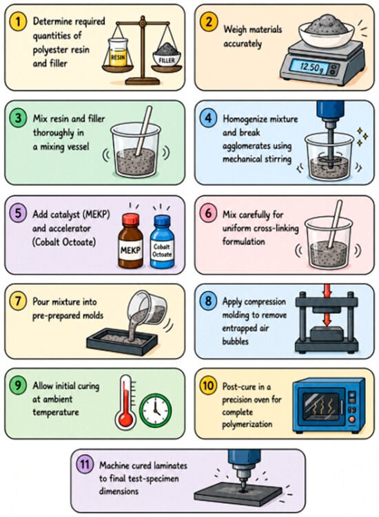
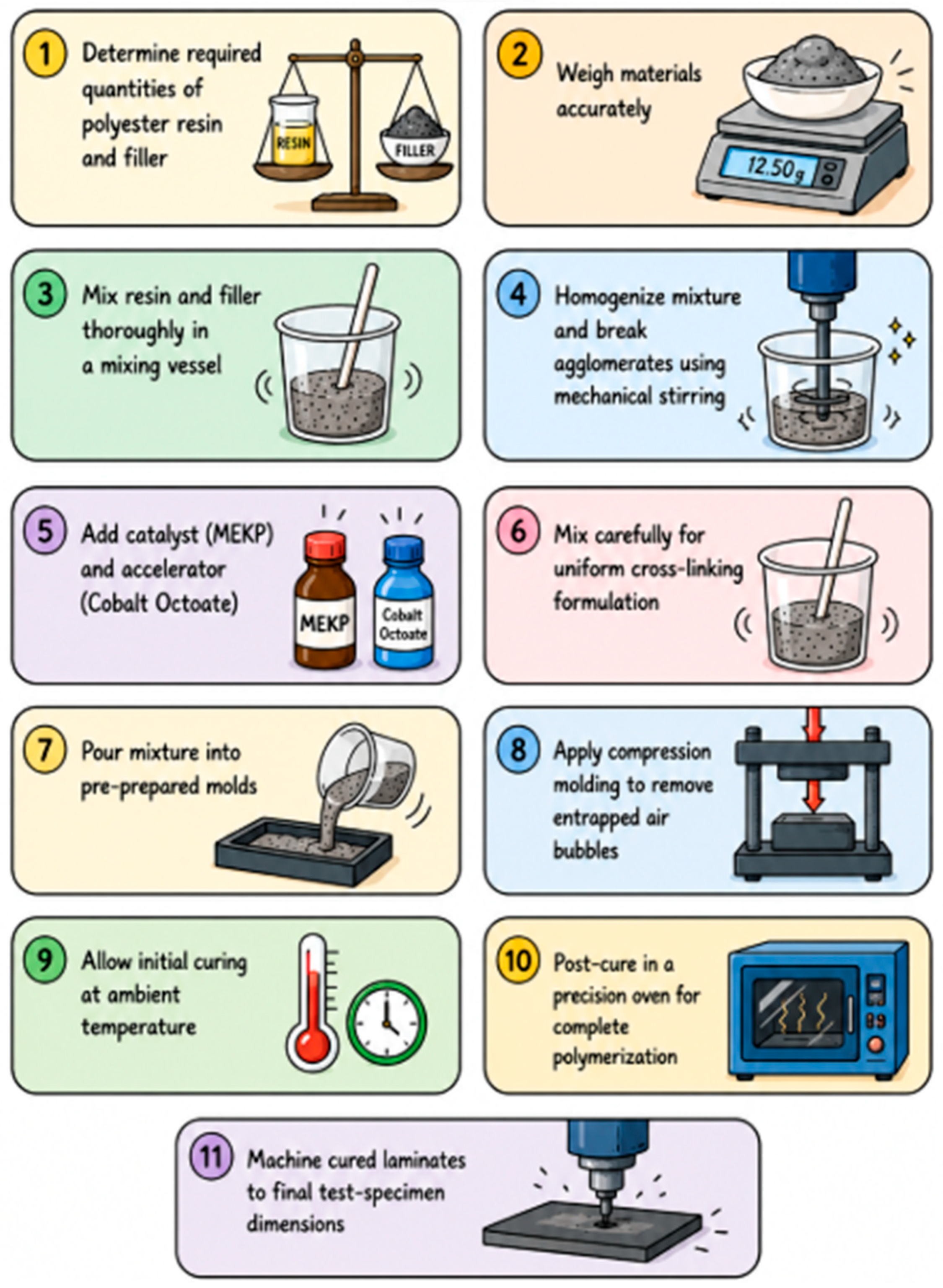
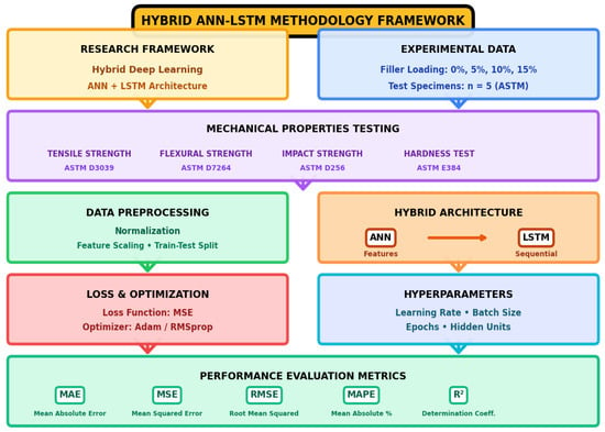
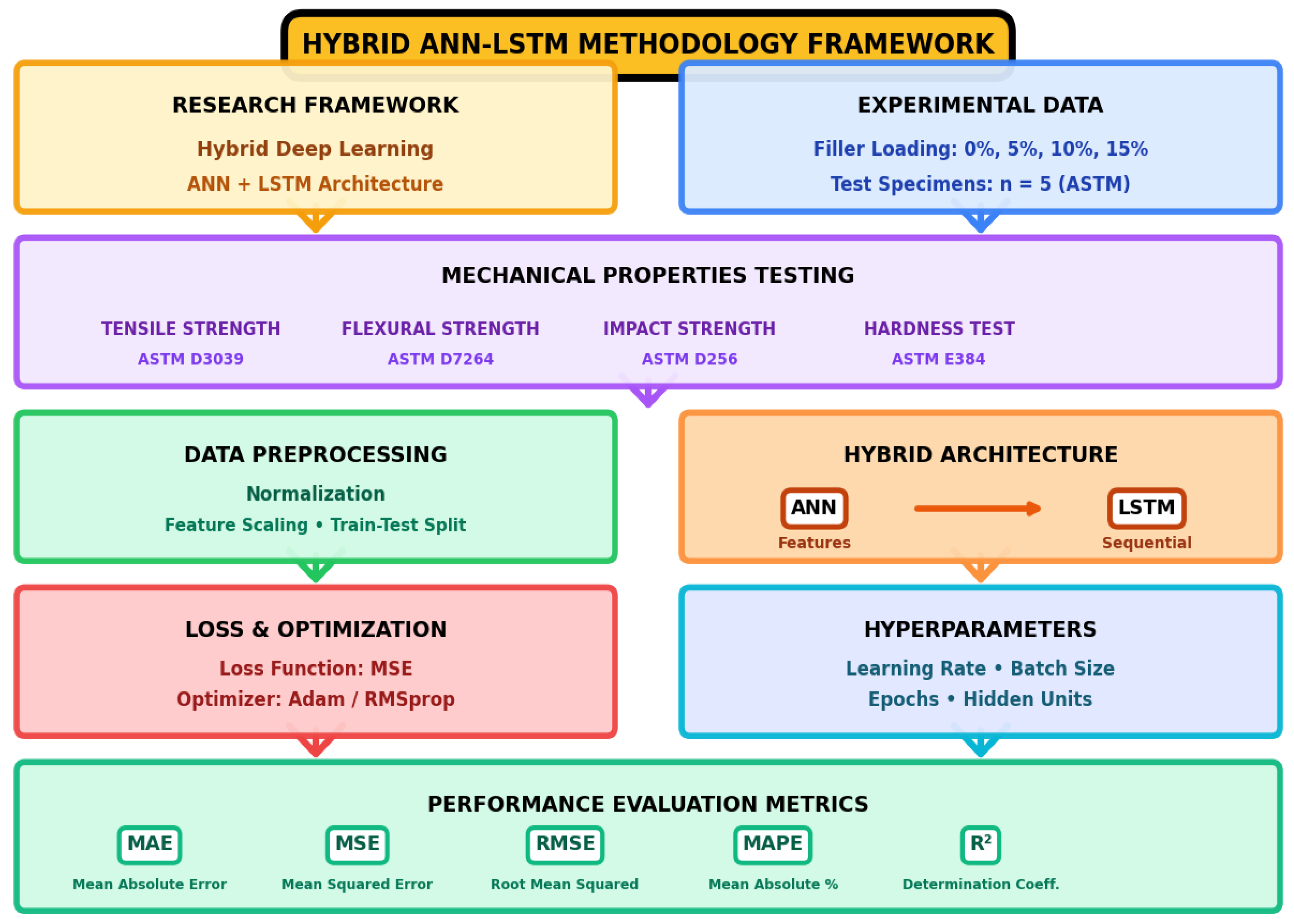
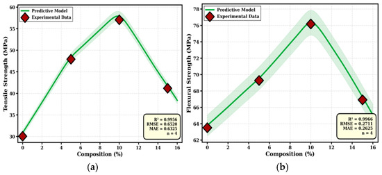
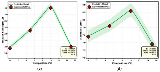
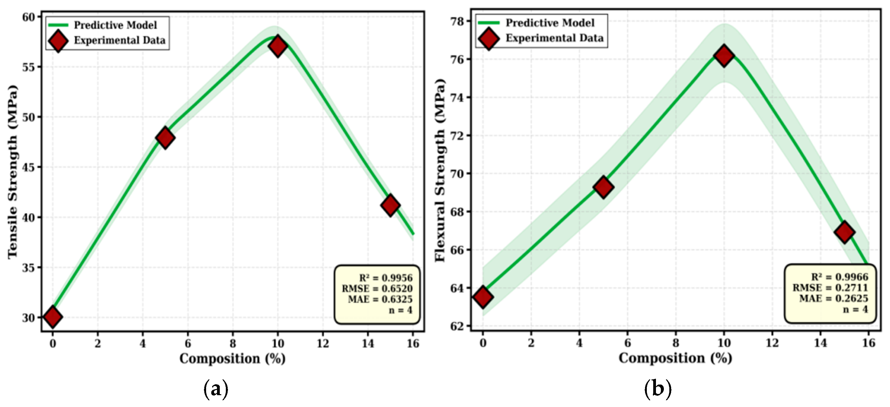
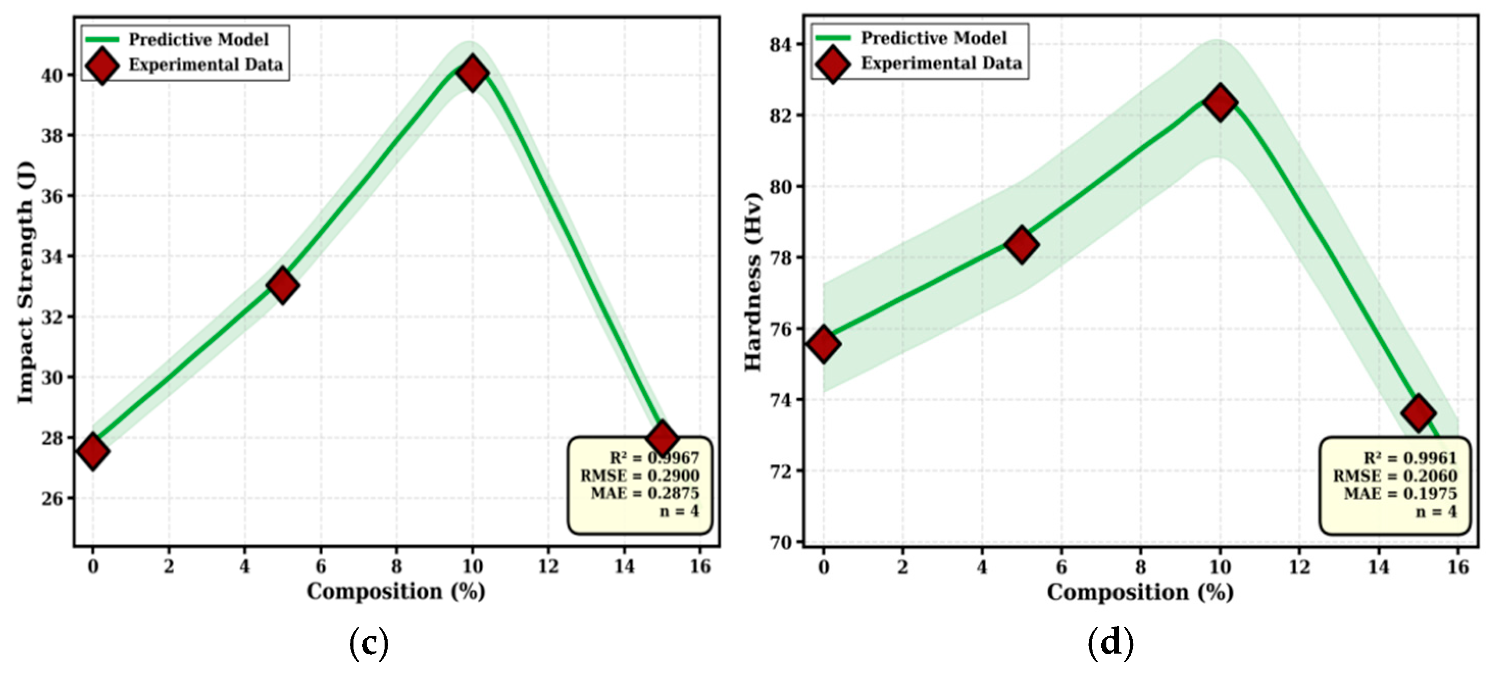
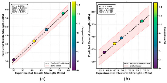
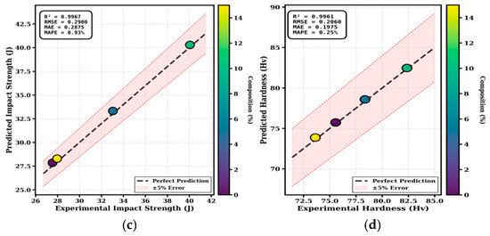
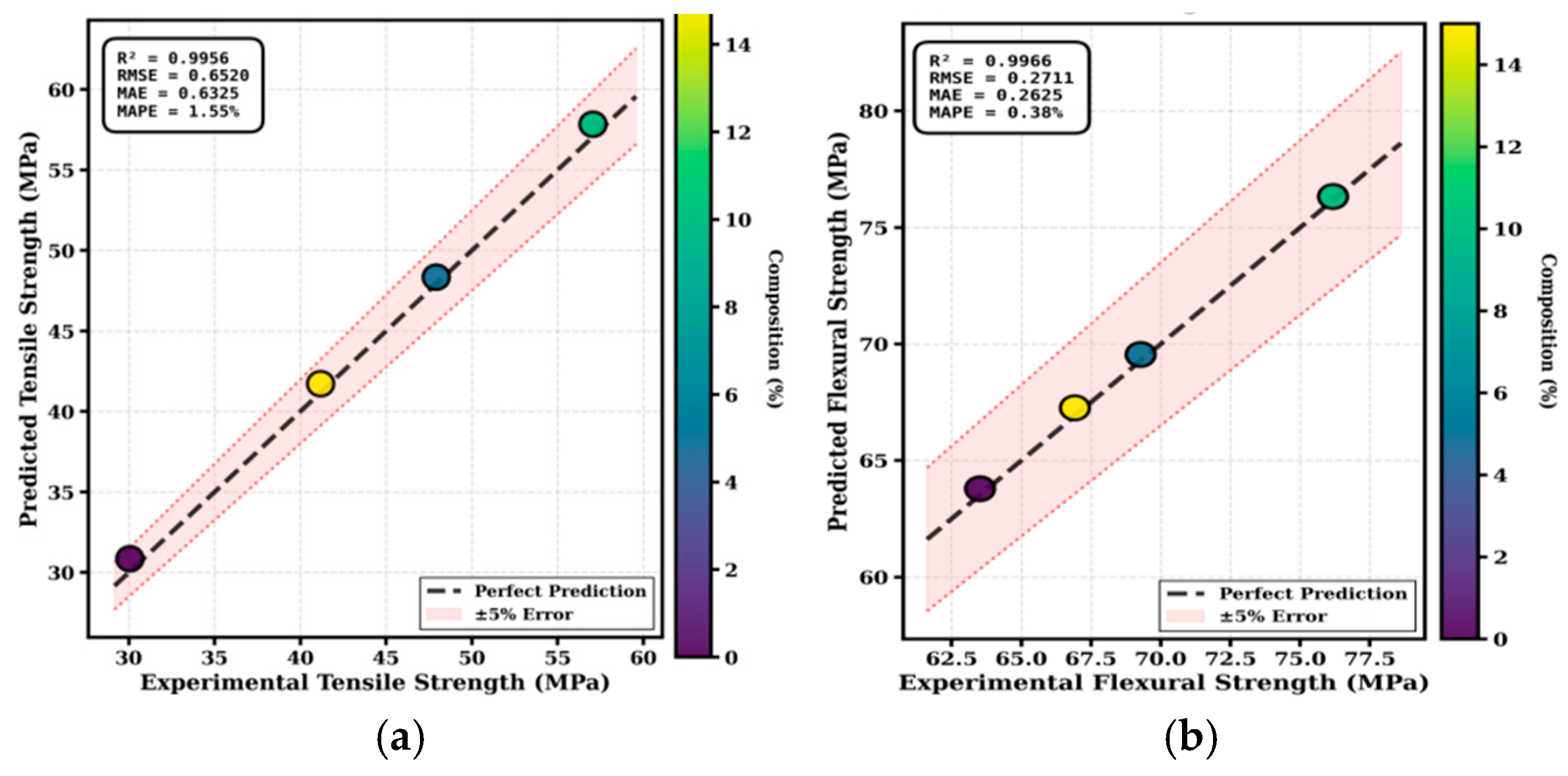
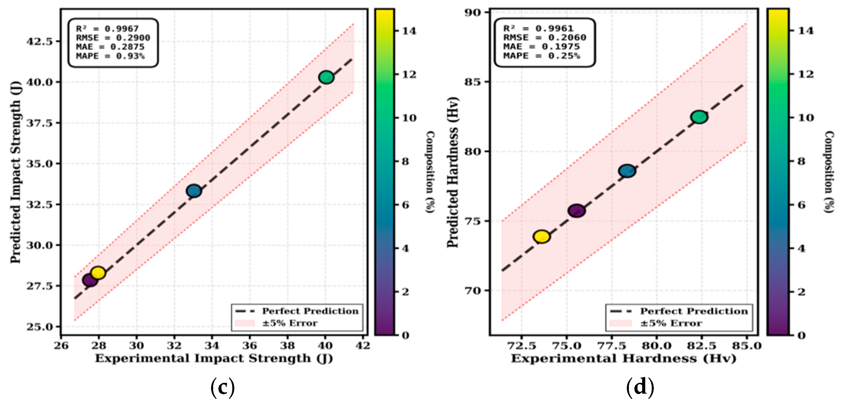
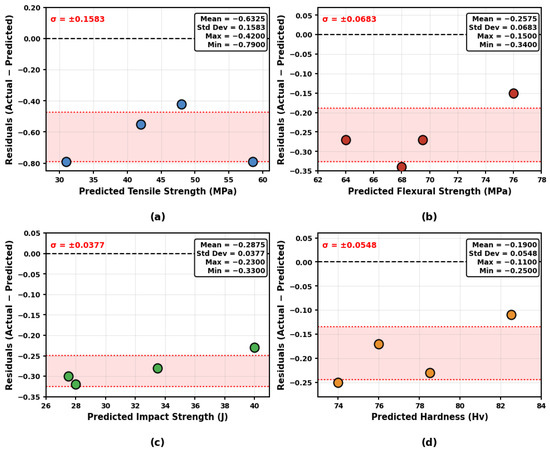
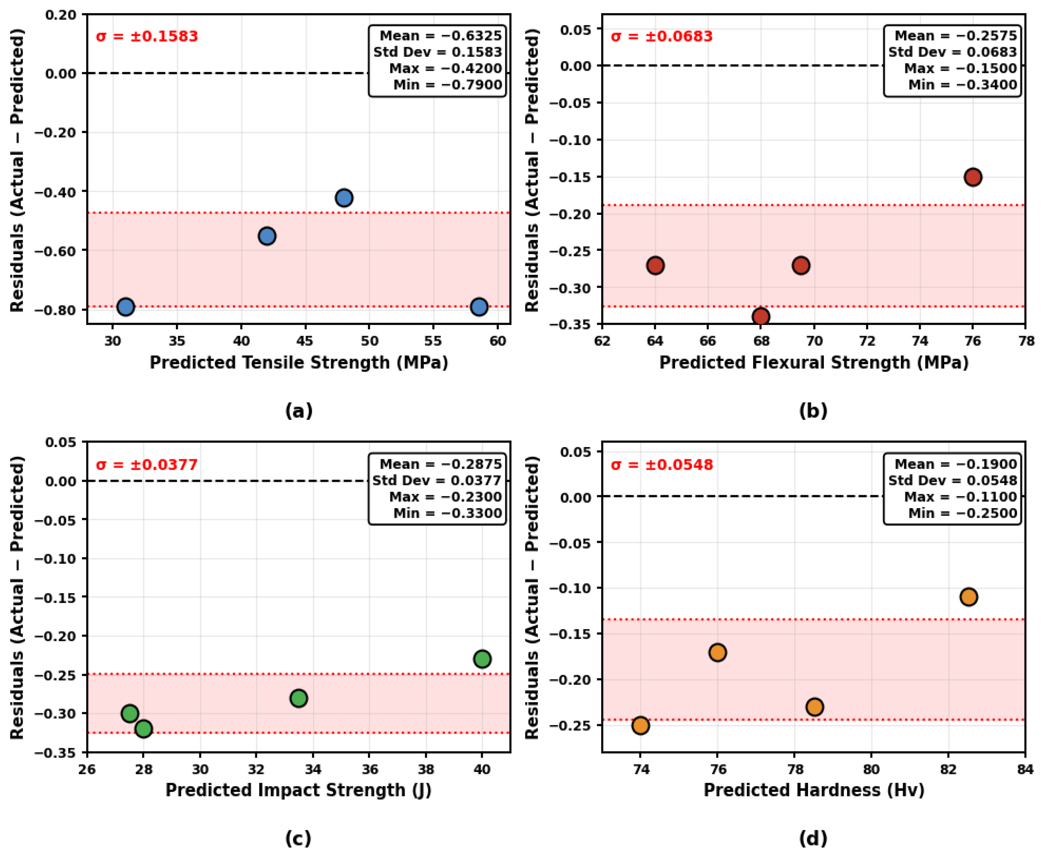
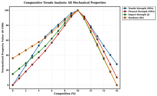
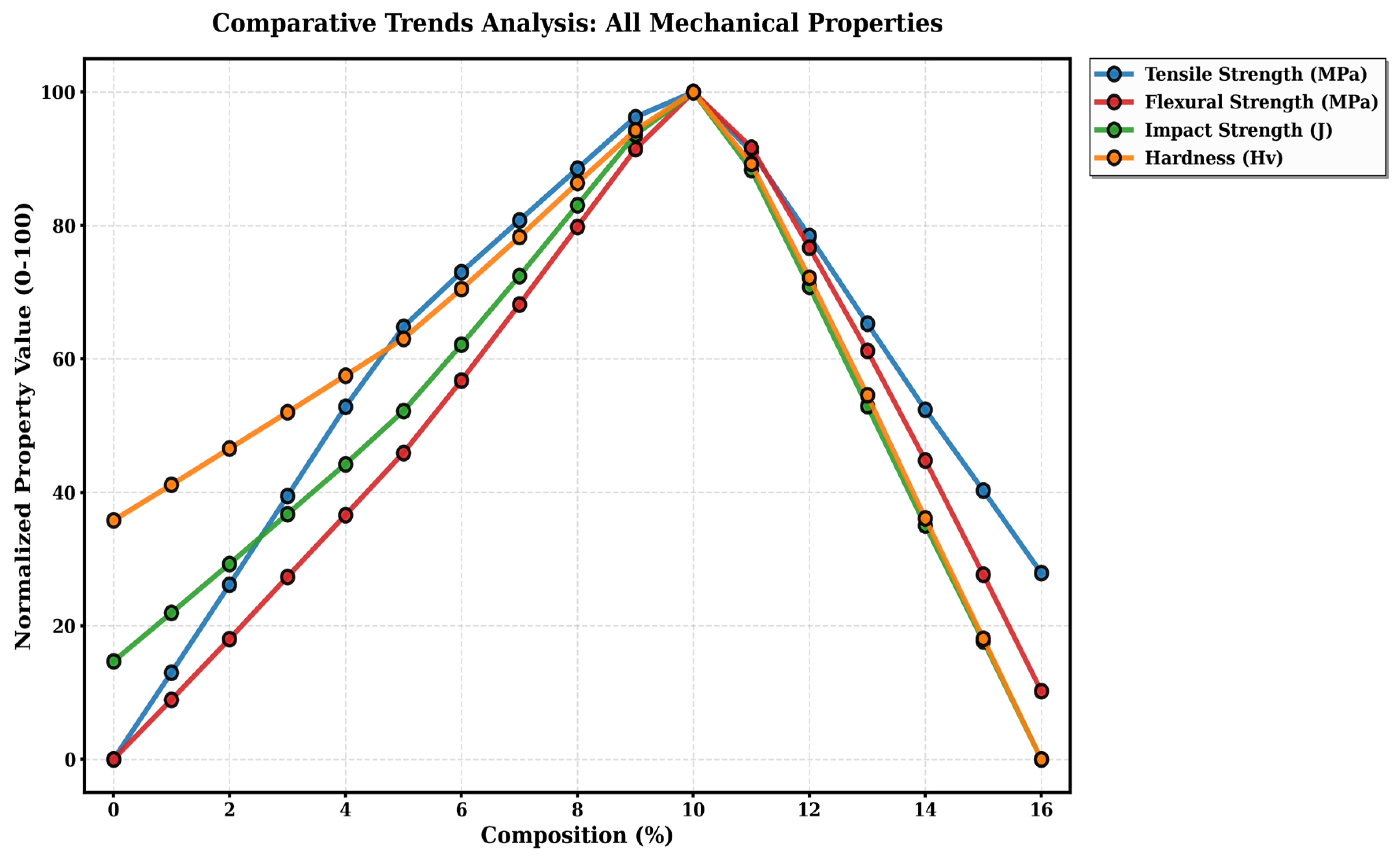
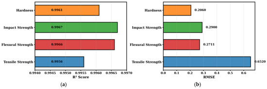
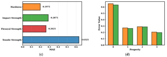
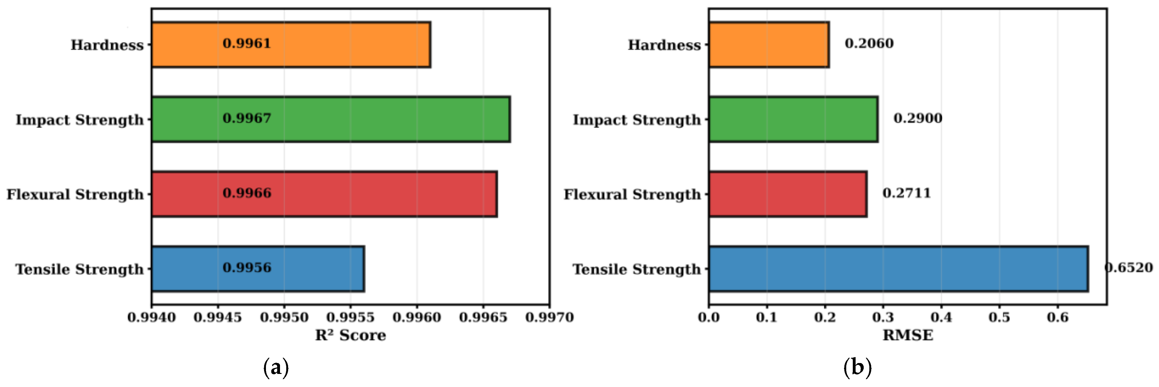
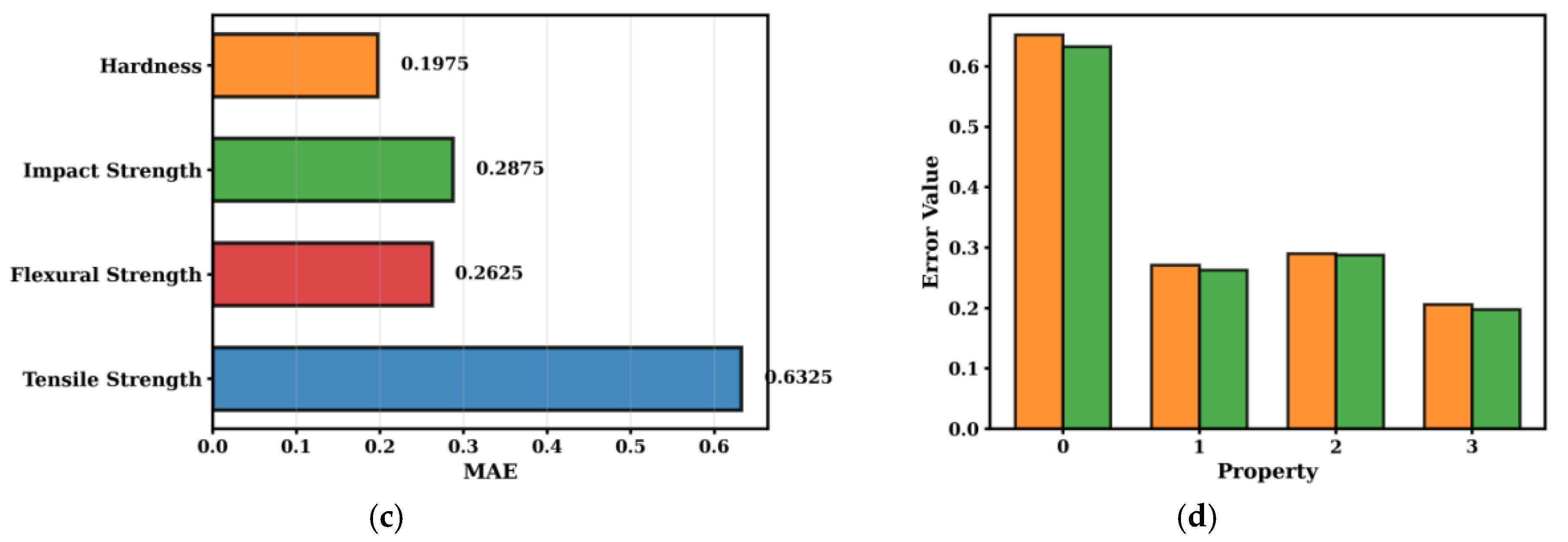

Disclaimer/Publisher’s Note: The statements, opinions and data contained in all publications are solely those of the individual author(s) and contributor(s) and not of MDPI and/or the editor(s). MDPI and/or the editor(s) disclaim responsibility for any injury to people or property resulting from any ideas, methods, instructions or products referred to in the content. |
© 2026 by the authors. Licensee MDPI, Basel, Switzerland. This article is an open access article distributed under the terms and conditions of the Creative Commons Attribution (CC BY) license.