


Abstract
People suffering from chronic diseases like diabetes, heart disease, and Parkinson’s disease are reliant on their implantable devices to improve their quality of life and to manage their chronic conditions. Despite their advantages, some systems are battery-powered, which can lead to battery failure, resulting in prophylactic surgery. One solution to this issue is an implantable antenna that provides an adequate link margin across various skin sites. In this study, we introduce an implantable antenna design optimized using an open-source PSO algorithm. The antenna is a tunable WMTS-motivated design fabricated on a Rogers 6010.2 substrate and evaluated by simulation and in vitro testing using phantom tissues. Validation measurements are performed to evaluate the effects of implantation depth across various adipose thicknesses.
1. Introduction
On 11 October 2016, St. Jude Medical (SJM) and the Food and Drug Administration (FDA) released a global medical device letter advisory announcing the risk of premature battery depletion found in some implantable cardioverter defibrillator (ICD) and cardiac resynchronization therapy defibrillator (CRT-D) devices. These implantable medical devices (IMDs) powered by lithium-based battery clusters have been found to create abnormal electrical connections, leading to rapid battery failure and early battery depletion. According to the report, 398,740 affected devices were sold worldwide, with 349,852 devices actively implanted and 841 devices returned for evaluation. As a result, 0.24% of the evaluated IMDs were discovered to have premature battery depletion due to lithium cluster failure. The battery system exacerbates the patient’s health, resulting in thirty-seven patients suffering from dizziness, ten patients from fainting, and two patients dying due to battery depletion. Despite the Class I recall and health risks, patients desperately need their ICD and CRT-D. The SJM, the FDA, and the Indian Heart Rhythm Society committee do not recommend prophylactic surgical procedural replacement unless the devices show evidence of battery depletion problems [1]. The battery system is a major component of these pacemakers, delivering electrical pulses that stimulate the lower chambers of the heart to resynchronize its natural rhythm and mitigate irregular heart rhythms associated with heart failure.
Recent IMDs have remedied the need for invasive prophylactic surgery from battery failure by substituting permanent batteries for wireless power delivery systems. For example, the FDA has approved subcutaneous IMDs, such as deep brain stimulation (DBS) [2], and continuous glucose monitoring (CGM) systems [3] for patients suffering from Parkinson’s disease and diabetes. While DBS IMD provides electrical pulses to the brain to treat Parkinson’s symptoms, the system requires patients to wear a relatively large, weighted, over-the-neck device to wirelessly power and charge the sensor implanted within the chest [2]. Meanwhile, CGM IMDs provide patients with the convenience of actively monitoring their blood glucose levels by requiring them to wear a relatively large modem that wirelessly powers the sensor implanted in the upper arm [3]. Despite the advances of these systems, the wireless power transfer systems for these IMDs are explicitly designed for their target skin site. One solution to address these limitations is a wireless power transfer antenna design suitable for various skin sites. Such antennas must be relatively small, be made of biocompatible materials, provide adequate link margin across various skin sites, and accommodate the dielectric properties of tissues among individuals with different body compositions.
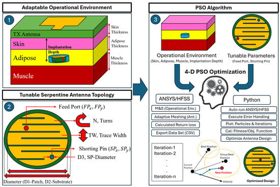
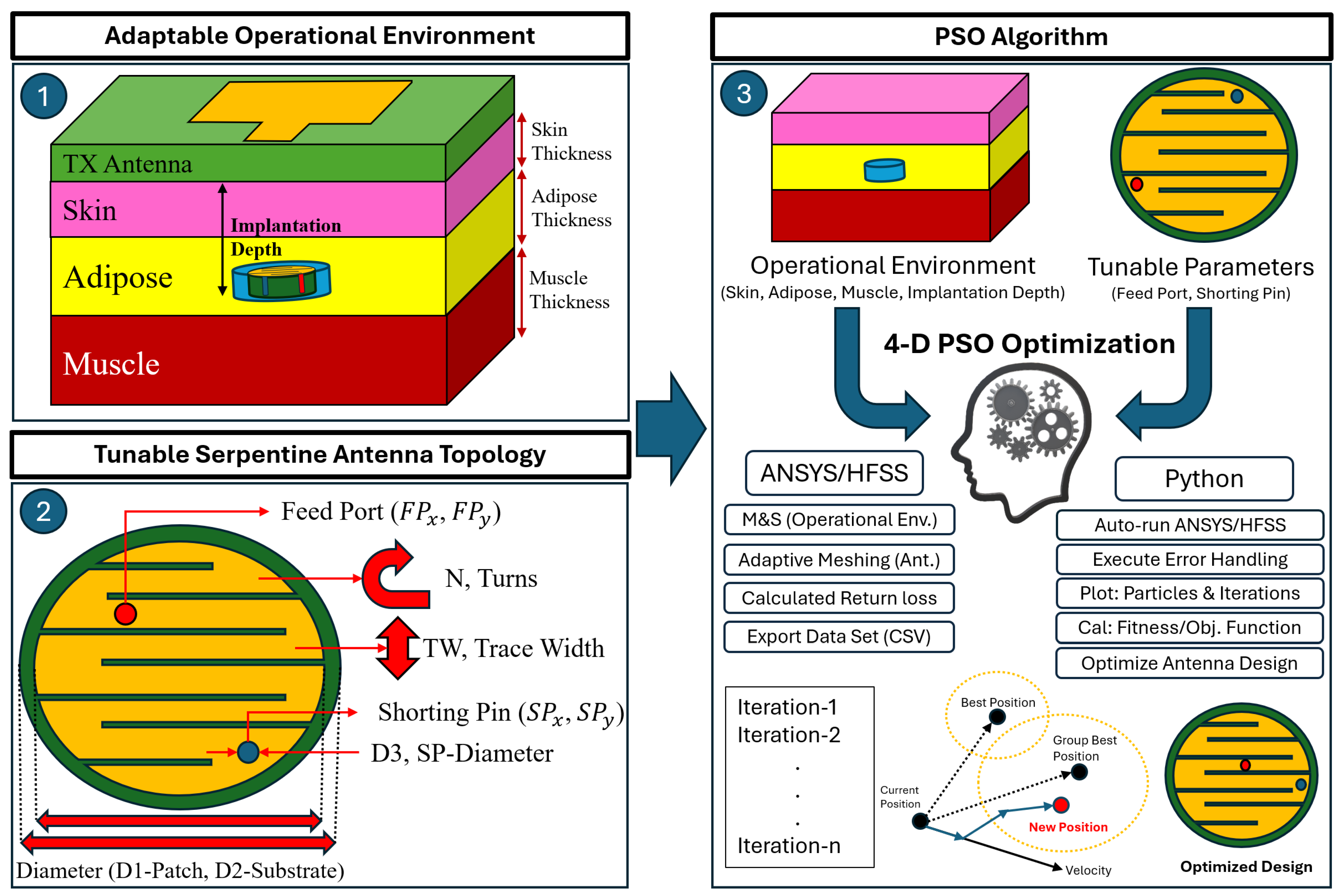
In this study, we introduce an implantable antenna design optimized using an open-source particle swarm optimization (PSO) algorithm (Figure 1). This paper presents the design, pseudocode, simulation, and fabrication of an implantable antenna. The antenna design topology is tunable and can be adjusted to various skin sites and body compositions. The antenna is a WMTS-motivated design and is encapsulated within a biocompatible MDX4-4210 silicone. This paper presents in vitro testing, evaluating antenna performance in terms of gain, return loss (), and insertion loss () across various adipose phantom thicknesses.
Figure 1.
A three-stage approach to optimize an implantable antenna design using a PSO algorithm.
1.1. Related Works
Contrary to a traditional antenna operating in a lossless free-space environment, the operational environment for implantable antennas is dynamic and challenging to characterize. The electrical properties of human tissues, biocompatible enclosures, tissue thicknesses, and implantation depths are just a few factors that can affect antenna performance. In recent years, researchers have designed implantable antennas by employing a superstrate to miniaturize the antenna’s footprint while incorporating meandering antenna topology with the feeding port and shorting pin of various sizes at designated positions to obtain a desirable resonance frequency [4,5,6,7,8,9,10,11].
Due to the complex biological environment, researchers have introduced new methods to incorporate machine learning (ML) optimization techniques into antenna designs for biomedical applications [7,9,10,12]. Rasool Khan et al. deployed supervised ML techniques such as support vector regression (SVR), decision trees (DT), random forests, artificial neural networks (ANNs), and Gaussian regression to optimize an on-body antenna design [12]. Meanwhile, Hood et al. and Karacolak et al. have integrated an unsupervised algorithm, such as PSO, to optimize the design of an implantable antenna [7,9,10]. Despite these demonstrated advantages, few implantable antenna studies address the variability of skin sites and implantation depth and their effects on antenna performance.
Moreover, recent studies validate the antenna design using on-body human test subjects [13], homogeneous human scalp phantoms [4,8], and in vivo/ex vivo animal models [11,14,15]. Compared with other studies, tissue phantoms allow for reliable and consistent measurements over fresh protein and human scalp phantom. Validating an antenna design through in vitro testing using tissue phantom minimizes potential risks to human subjects and harm to animal test subjects. More importantly, tissue phantoms can be fabricated to various thicknesses, allowing for the replication of targeted skin sites.
1.2. Contributions
While some studies have deployed ML supervised (SVR, DT, random forests, ANN, Gaussian regression) [12] and unsupervised PSO techniques for biomedical antenna designs [7,9,10], these studies are tailored to a specific targeted skin site and desired resonance frequency, which has reduced their adaptability for application to other skin sites and variations in body composition.
The main contribution of this study is the design of a circular serpentine implantable antenna with an adjustable 4 Degrees-of-Freedom (DoF) operational environment and 6-DoF tunable parameters topology. The antenna is validated using tissue phantoms, and food products are proposed as substitutes for an adipose tissue phantom. In addition, this work incorporates an open-source metaheuristic optimization framework that automatically interfaces with Ansys HFSS to tune a WMTS-motivated antenna design. Table 1 summarizes the contributions of this work and compares it with state-of-the-art studies. The key advantages of the proposed approach are summarized below.
Table 1.
Comparison with state-of-the-art literature for implantable antennas.
- Adjustable design: We present a tunable implantable antenna design that can be tailored to different skin sites, operating frequencies, and implantation depths. Compared with previous work, which sets boundary conditions for PSO variables’ optimization of a specific desirable frequency [7,9,10,13], this study demonstrates a proof of concept for a WMTS-motivated antenna design (Figure 1). As discussed in later sections, variables such as N-turns and -trace width are a short list of parameters that could be used to modify the patch design to achieve alternative operating wavelengths.
- Adipose tissue phantom substitutes: The skin site for IMDs is dependent on the underlying chronic condition. Furthermore, the tissue thicknesses at these skin sites can vary between people. To address the variation across skin sites and body compositions, we characterize two food products that are suitable substitutes for adipose tissue. The adipose tissue phantoms are fabricated into a thin, stackable sheet to achieve different thicknesses (5 mm to 17 mm), replicating the variability between skin sites and body compositions. In vitro measurements with phantom tissues are used to evaluate the insertion loss between two coupled antennas mimicking the testing conditions for wireless power transfer.
- Metaheuristic optimization:
- (a)
- Dynamic exploration and exploitation constants: Our work modifies the PSO algorithm variables like the exploration constant, , and exploitation constant, , which reduces computational time for convergence. The algorithm increases these constants with each iteration, without external input.
- (b)
- Multidimensional particles: The visual representation of a particle consisting of more than three dimensions is difficult to depict. A visualization method is introduced to represent particles with more than three dimensions, enabling the identification of trends and patterns in high-dimensional search spaces.
- (c)
- Open-source: Our work is open-source, and the source code is publicly available on GitHub v3.19. In contrast with prior studies, with code developed in MATLAB [7], in-house code [9], and API Python libraries such as SciKit and TensorFlow [12], this work is developed in Python with the standard libraries.
Although this study correlates with patients suffering with chronic illnesses and wireless power transfer, topics such as biosensors, animal and human testing, charging/super capacitors, and rectifier circuits are beyond the scope of this paper. Our work focuses on the proposed antenna design, the application of metaheuristic optimization, an adipose phantom substitute, and antenna coupling between human tissue phantoms.
2. Materials and Methods
2.1. Overview
As depicted in Figure 1, our study is compartmentalized into three stages: (1) adjusting the 4-DoF operational environment via implantation depth and thicknesses for the skin, adipose, and muscle tissues; (2) tuning of a 6-DoF serpentine implantable antenna design via D1, D2, FP, N, TW, and SP; and (3) optimizing the tunable serpentine implantable antenna using an open-source PSO algorithm. The first stage is to define the geometric parameters necessary to model specific skin sites. The following stage is to determine the shape and size of the circular serpentine antenna and select the particle’s tuning variables. The third stage is to apply PSO, which optimizes the implantable antenna design and plots multidimensional particle values for visual feedback. Afterward, the antenna design is validated via in vitro testing, which is discussed in the measurements and results section.
2.2. Characterizing the Operational Environment
2.2.1. Adjustable Operational Environment
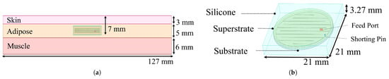
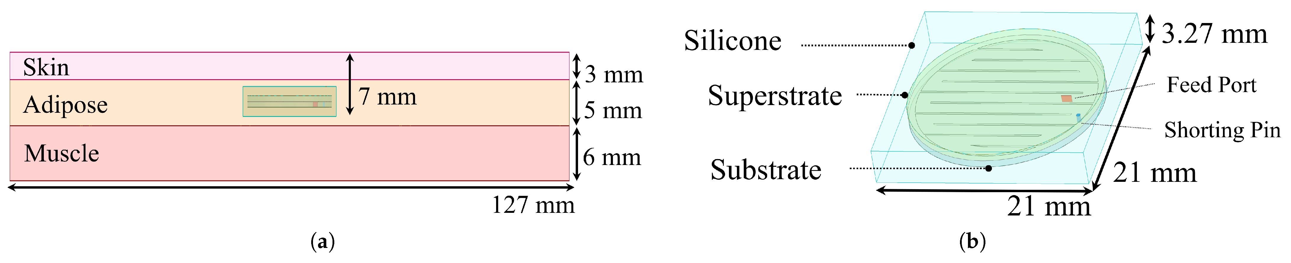
Traditionally, IMD antennas are simulated using three distinct tissue layers: skin, adipose, and muscle tissues [10,11,16]. As shown in Figure 1 (stage 1), the operational environment for an IMD antenna can change with variations in skin site and body composition. By accounting for implantation depth and tissue thicknesses, the proposed design topology can be adjusted to most skin sites and variations in body composition. We modeled the operational environment in Ansys High Frequency Structure Simulator (HFSS) v2024 R1 by enclosing the serpentine antenna in silicone and implanting it 7 mm into the subcutaneous tissue (Figure 2a). Furthermore, the overall dimensions selected for the encapsulating silicone are 21 mm × 21 mm × 3.27 mm, providing a 1 mm spatial padding around the antenna design (Figure 2b). The tissue layers are modeled with a similar footprint (127 mm × 127 mm), but with varying thicknesses.
Figure 2.
Operational environment for IMD antennas: (a) tissue thickness and implantation depth and (b) antenna enclosure and silicone dimensions.
Although measurements for the epidermal range are from 0.05 mm to 0.1 mm in thickness and the dermal range from 0.5 mm to 5 mm, the average combined thickness for the cutaneous tissue (epidermal and dermis) is 2 mm [17]. To account for this variability, a conservative total skin thickness of 3 mm was selected for the human skin model. The variation in body composition between people can be primarily attributed to body mass index (BMI).
Adult obesity is commonly estimated using BMI, calculated as body mass (kg) divided by the square of height (m2). Underweight, normal weight, and overweight classifications correspond to BMI values of <18.5 kg/m2, 18.5 kg/m2–23 kg/m2, and 23 kg/m2–25 kg/m2, respectively. Several studies by Jain et al., Gibney et al., and Sim et al. used ultrasound to measure subcutaneous tissue layers in type-2 diabetic patients (N > 600) from the United States, South Korea, and India, establishing a representative average thickness for the human subcutaneous layer. Their findings show that adipose layer thickness increases with BMI. Based on these findings, we selected thicknesses of 3 mm, 5 mm, and 6 mm for the skin, adipose, and muscle tissues, respectively. These values reflect the average minimum adipose thicknesses of underweight adults with BMI < 18.5 kg/m2 at common anatomical sites, such as the upper arm, abdomen, and thigh [18,19,20].
The studies by Jain et al., Gibney et al., and Sim et al. show that the average adipose thickness of the upper arm for underweight and overweight adults ranges between 3.9 mm and 12.82 mm, while the adipose thickness of the abdomen ranges from 5.18 mm to 16.56 mm. The average thickness of the thigh ranges from 4.89 mm to 12.44 mm [18,19,20]. To address this variability, an initial adipose thickness of 5 mm was conservatively selected and incrementally increased in 2 mm steps up to 19 mm. As discussed in later sections, adipose phantoms are fabricated as 2 mm thick sheets for in vitro testing to evaluate the effects of implantation depth across different skin sites and body compositions.
2.2.2. Fabrication and Characterization of Tissue Phantom
Human tissue phantoms and biologically compatible silicone are fabricated and characterized to validate simulation and to evaluate antenna performance. Tissue-mimicking gels minimize risks to both animal and human test subjects while providing reliable, consistent measurements [9]. However, adipose tissue-mimicking gels can be difficult to fabricate due to their oily composition, which is sensitive to heat and lacks the ability to hold their shape when fabricated thinly. To address this issue, we evaluated butter and lard as potential substitutes for modeling human adipose tissue across 5 mm and 19 mm. Butter and lard exhibit dielectric properties similar to those of human adipose tissue, making them suitable substitutes [21]. Similarly, silicone rubber is a viable substitute for DuPont MDX4-4210 biomedical-grade elastomer silicone because it exhibits similar physical and dielectric properties.
Sodium chloride, vegetable oil, and de-ionized water are among the main ingredients used to replicate the electrical properties of human skin, adipose, and muscle tissues. Sodium chloride is used to increase the conductivity, , while decreasing the relative permittivity, , for tissue phantoms. Meanwhile, de-ionized water exhibits high , while vegetable oil exhibits low . Furthermore, gelatin type A (porcine), gelatin type B (bovine), Ultra Ivory hand soap, Triton-X100, and food coloring are used in small concentrations to solidify the ingredients into a gel. The small volumetric concentration of these gelatin-based ingredients has little electrical effect on tissue-mimicking gels [22]. Table 2 lists the U.S. sourced phantom gel ingredients, along with the solute amounts in proportion to a 100 mL volumetric solution. The liquid mixtures were poured into custom molds, covered, and refrigerated overnight to solidify into tissue-mimicking gels.
Table 2.
Tissue-mimicking gel recipe.
Food products such as frozen butter and lard exhibit similar electrical properties as human adipose tissue [21]. U.S. sourced Land O’Lakes salted butter and John Morrell Snow Cap Manteca lard were selected as suitable substitutes over adipose tissue-mimicking gel. The butter and lard were spread into 2 mm thin flexible molds at ambient temperature, and then placed in the freezer to harden.
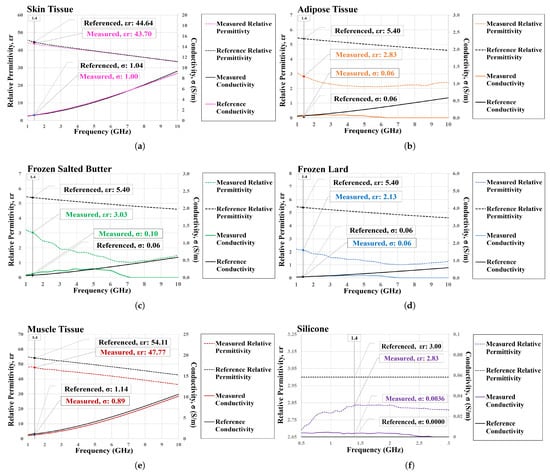
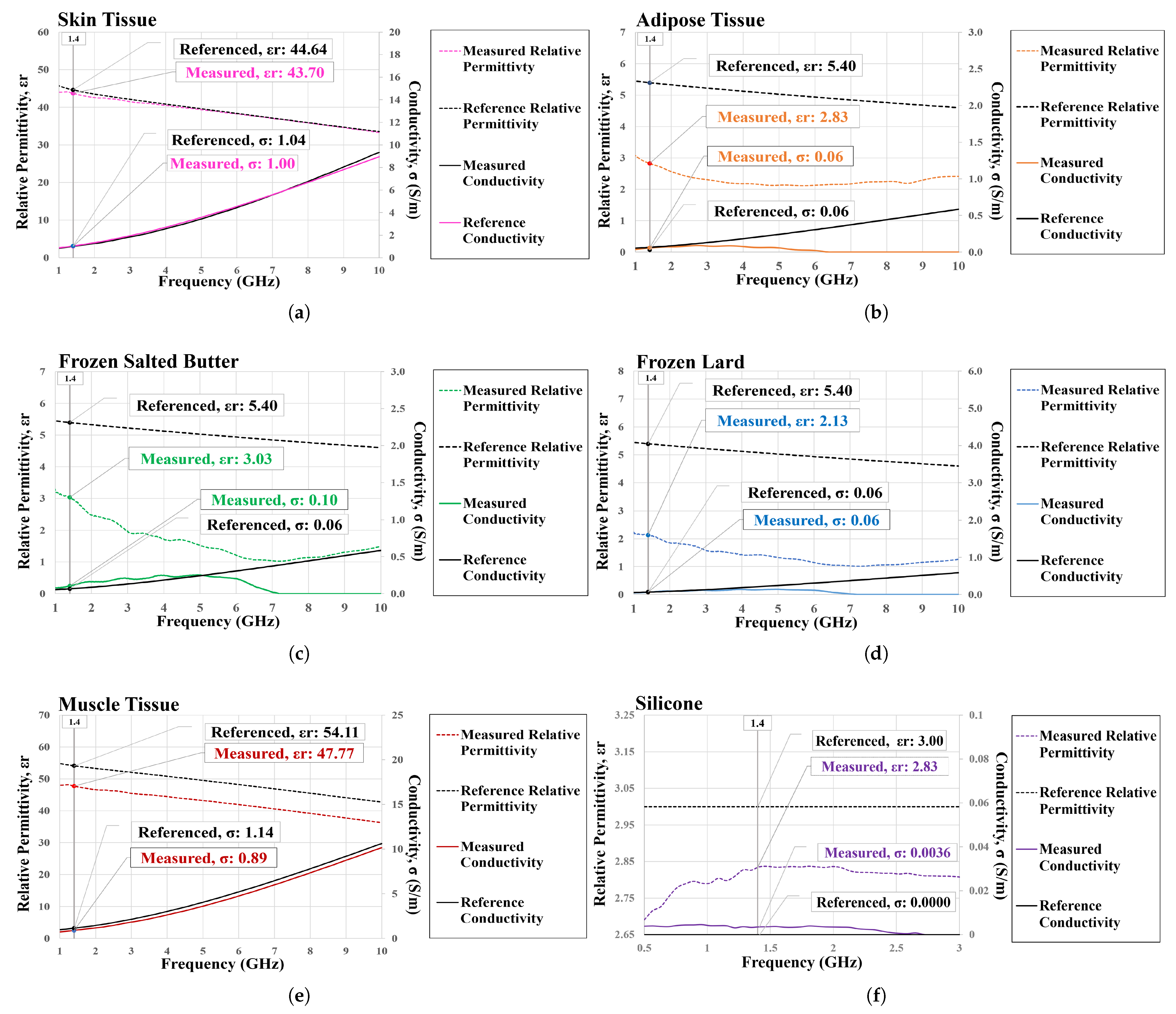
Benchtop testing was performed to characterize the dielectric properties of materials necessary for in vitro testing. Using an Agilent E8362B PNA network analyzer with a Keysight N1501A probe, and were measured between 1 GHz and 10 GHz for completeness. As shown in Figure 3, (dotted lines) and (solid lines) plotted trend lines for the tissue phantom overall agree with the reference Cole–Cole plots [23].
Figure 3.
Comparison of dielectric property for selected materials: (a) skin tissue-mimicking gel, (b) adipose tissue-mimicking gel, (c) frozen salted butter, (d) frozen lard, (e) muscle tissue-mimicking gel, and (f) silicone rubber.
In Figure 3a, the trend line for the measured dielectric properties of the phantom skin, which is outlined in pink ( = 43.70, = 1.00), agrees with the reference plot outlined in black ( = 44.64, = 1.04). Similarly, Figure 3b shows that the trend lines for the measured dielectric properties of phantom adipose, which is outlined in orange ( = 2.83, = 0.59), agrees with the reference plot outlined in black ( = 5.40, = 2.83). Additionally, Figure 3e plots the dielectric properties of phantom muscle line outlined in red ( = 47.77, = 0.89), and its trend lines agree with the reference plot outlined in black ( = 54.11, = 1.14). Lastly, the dielectric properties of Let’s resin silicone rubber (Figure 3f) were measured using the same methods, yielding = 2.83 and = 0.0036. The plotted trend line agrees with the MDX4-4210 reference plot ( = 3.00 and = 0) between 1 GHz and 3 GHz [5].
Figure 3c shows that the measured dielectric properties for frozen Land O’Lakes salted butter, outlined in green, were plotted ( = 3.03, = 0.10), and its trend lines agree with the reference plot ( = 5.40, = 0.06). Likewise, the measured frozen lard outlined in blue lines in Figure 3d ( = 2.13, = 0.06) shows trend lines that agree with the reference plot ( = 5.40, = 0.06). Although measured frozen butter, frozen John Morrell Snow Cap Manteca lard, and adipose tissue-mimicking gel have similar dielectric properties, the physical aspects of adipose gel and frozen butter are prone to cracking and breakage, resulting in air gaps when fabricated into thin molds less than 3 mm thick. Unlike frozen salted butter and adipose gel, frozen lard can be spread consistently thin and can be removed from thin molds due to its pliable and homogeneous physical attributes.
2.3. Antenna Designs
2.3.1. Implantable Antenna Design
To meet the design constraints for IMD applications, we selected a circular serpentine patch antenna topology. This design topology type is favorable due to its versatility, low profile, and compact footprint [5,8,9,11,15]. As shown in Figure 1, the design topology has six directions of motion/6-DoF, resulting in nine tunable parameters: , , , , N-number of turns, -trace width, -substrate diameter, -patch diameter, and -shorting pin diameter.
As shown in Table 3, the substrate and superstrate are made from Rogers 6010.2 H1/H1 LM (, ) PCB material with a thickness of 0.025 in and are enclosed in DuPont MDX4-4210 silicone (). The Rogers 6010.2 substrate exhibits high dielectric properties, which are beneficial for the miniaturization of antenna designs. The overall size of the antenna is constrained to a 19 mm diameter with a thickness of 0.762 mm, which is comparable to the size of a U.S. dime or penny. The trace width and continuous serpentine loops (N-turns) are 1.4 mm and 11, respectively. The parameters for the trace width and N-turns are selected to ensure that the slots between the traces are greater than two mils and the serpentine length is greater than 2. Besides these fixed design constraints, the (x, y) feed port and shorting pin positions are tuning parameters that adjust the impedance and electrical length.
Table 3.
Implantable antenna dimensions.
2.3.2. Antenna Coupling
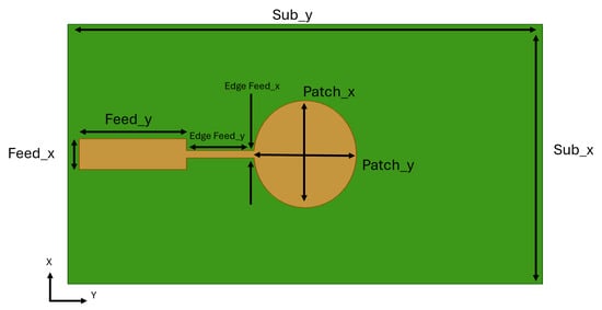
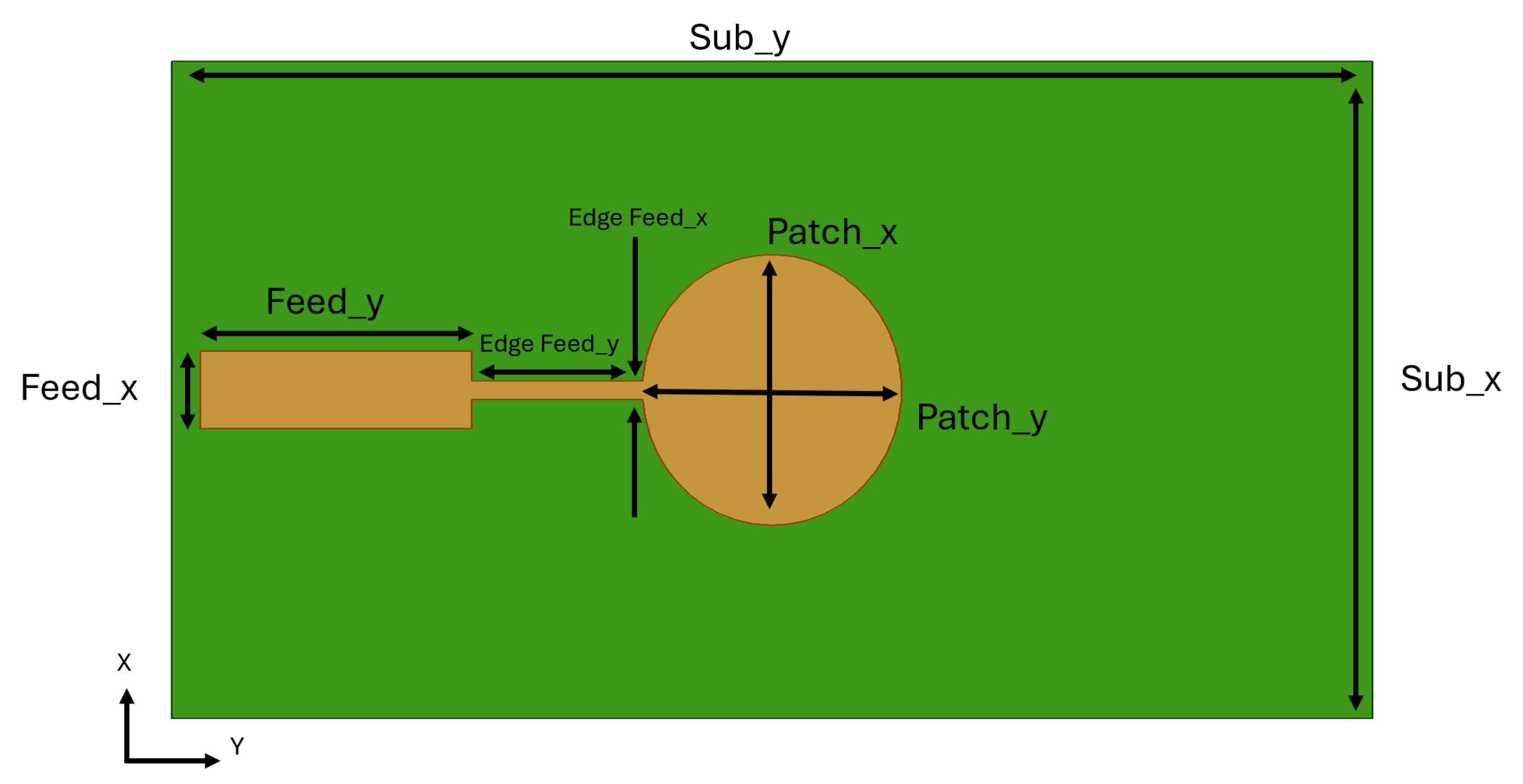
Two mutually coupled antennas are necessary to study the effects of implantation depth. In addition to implantable antenna design, a matching inverted antenna placed above the skin is essential for measuring the insertion loss between tissue. Inspired by [24], we selected an elliptical-edge feed patch antenna favorable for its tuning parameters and ease of manufacturing. The elliptical-edge feed patch must match the wavelength of the implantable antenna within the skin. The wavelength in the skin is calculated using Equation (1), in which c represents the velocity of light; (Figure 3a) denotes the relative permittivity of the skin at 1.4 GHz; and represents the operation frequency of 1.4 GHz.
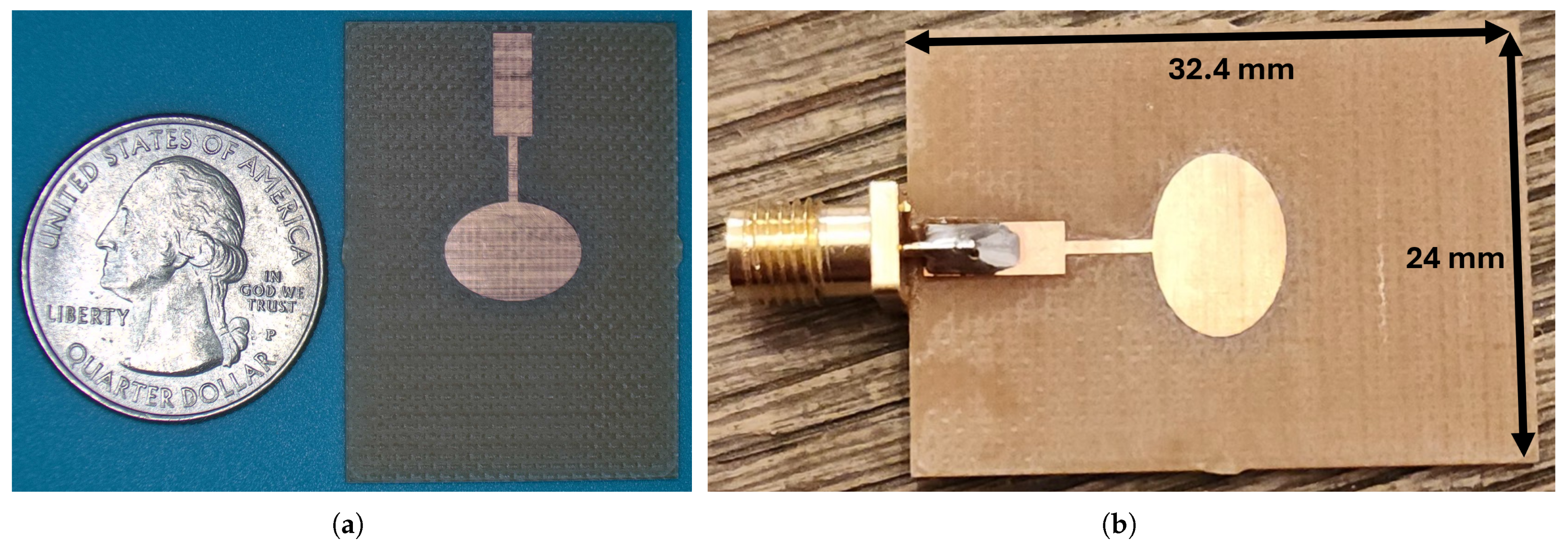
As shown in Figure 4, the parameters for the elliptical-edge feed patch antenna were tuned to achieve the calculated wavelength ( = 3.201 cm). The mutually coupled antenna was modeled in Ansys HFSS with the parameters shown in Table 4. The mutually coupled antenna is fabricated from a double-sided 1 oz copper-clad FR-4 PCB (, ), yielding an overall dimension of 32.4 mm × 24 mm × 1.6 mm.
Figure 4.
Antenna coupling-elliptical patch antenna design.
Table 4.
Elliptical antenna dimensions.
2.3.3. Fabrication of Antennas and Holding Apparatus
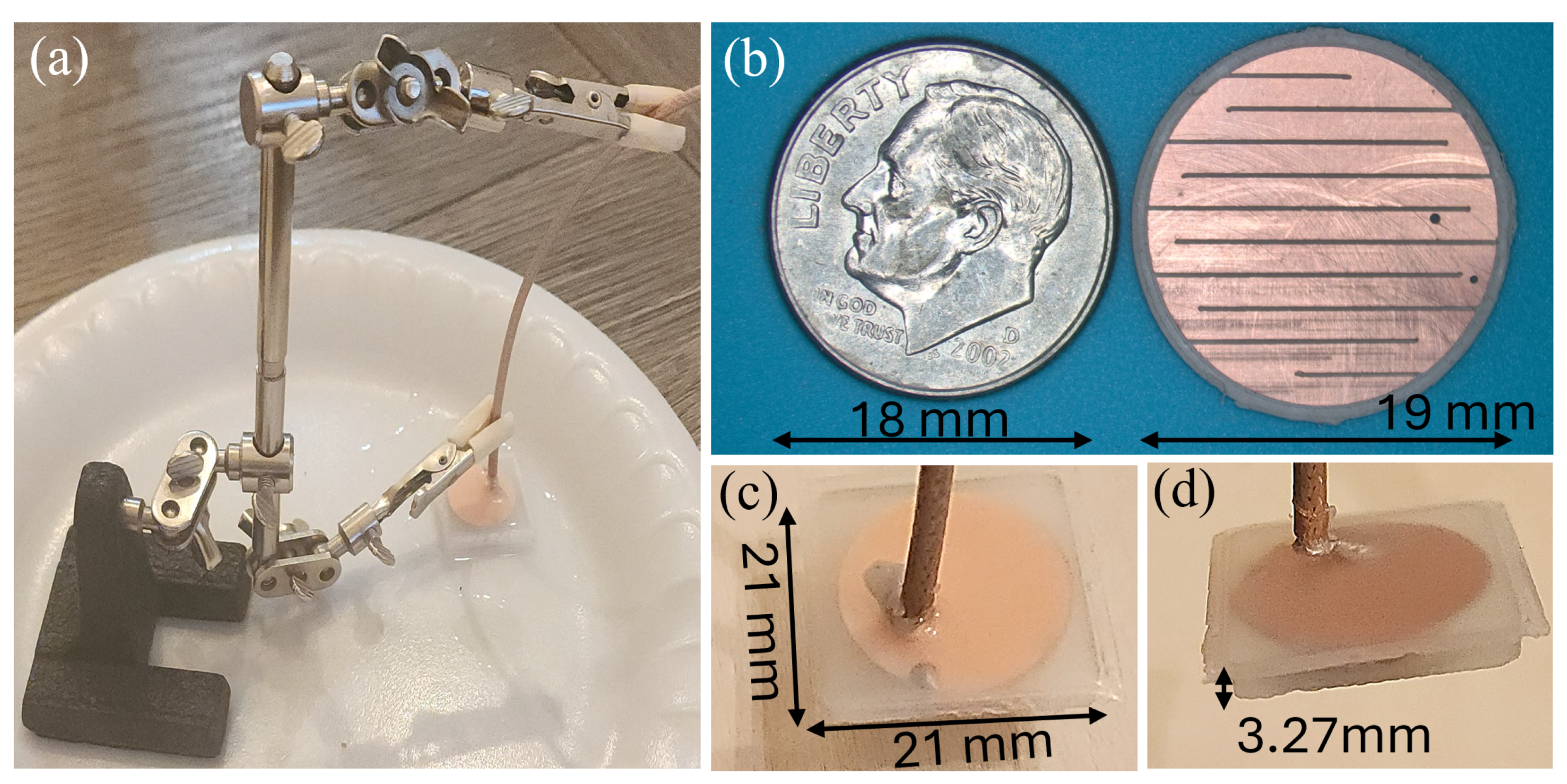
An LPKF Protomat S103 PCB milling machine was used to fabricate the implantable (substrate and superstrate) and elliptical antenna designs. As shown in Figure 5b, the implantable antenna has a similar footprint (19 mm × 1.27 mm) to a U.S. dime (18 mm × 1.35 mm). After the milling process, the shorting pin, made of solid 26 AWG (0.40 mm) copper conductor, and the feed port, made from the center conductor of an RG-316 coaxial cable, were soldered to the implantable antenna design.
Figure 5.
Implantable antenna fabrication: (a) antenna embedded in silicone and (b) milled design on Rogers 6010.2 substrate. IMD antenna enclosed in silicone: (c) top view and (d) side view.
Using a paintbrush, a thin layer of silicone rubber was applied to the exterior of the substrate and superstrate, bonding them together. After the thin layer had dried, silicone was poured into a negative mold. The mold was fabricated from flexible TPU and 3D-printed using a Bambu Lab H2D. As shown in Figure 5a, the antenna was submerged in the mold, with clamps used to secure the implantable antenna, which established a 1 mm clearance as well as ensuring that the SMA cable remained vertical. Silicone rubber was then poured into the mold, and the silicone was allowed to cure overnight. The flexible mold peeled freely from the silicone rubber, as seen in Figure 5c,d.
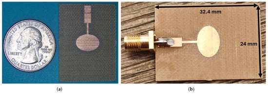
Similarly, the elliptical-edge feed patch antenna (Figure 6a) was fabricated using an LPKF Protomat S103 PCB milling machine, and its size (32.4 mm × 24 mm × 1.6 mm) is relatively larger than a U.S. quarter (24.3 mm × 1.6 mm). As shown in Figure 6b, the center pin of an edge mount female SMA was soldered to the edge feed. Afterward, the SMA connector’s outer pins were soldered to the elliptical antenna’s ground plane.
Figure 6.
Fabricated elliptical antenna: (a) referenced size and (b) soldered SMA.
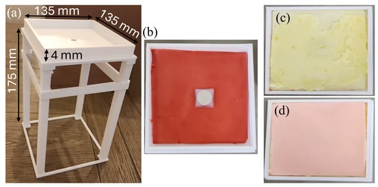
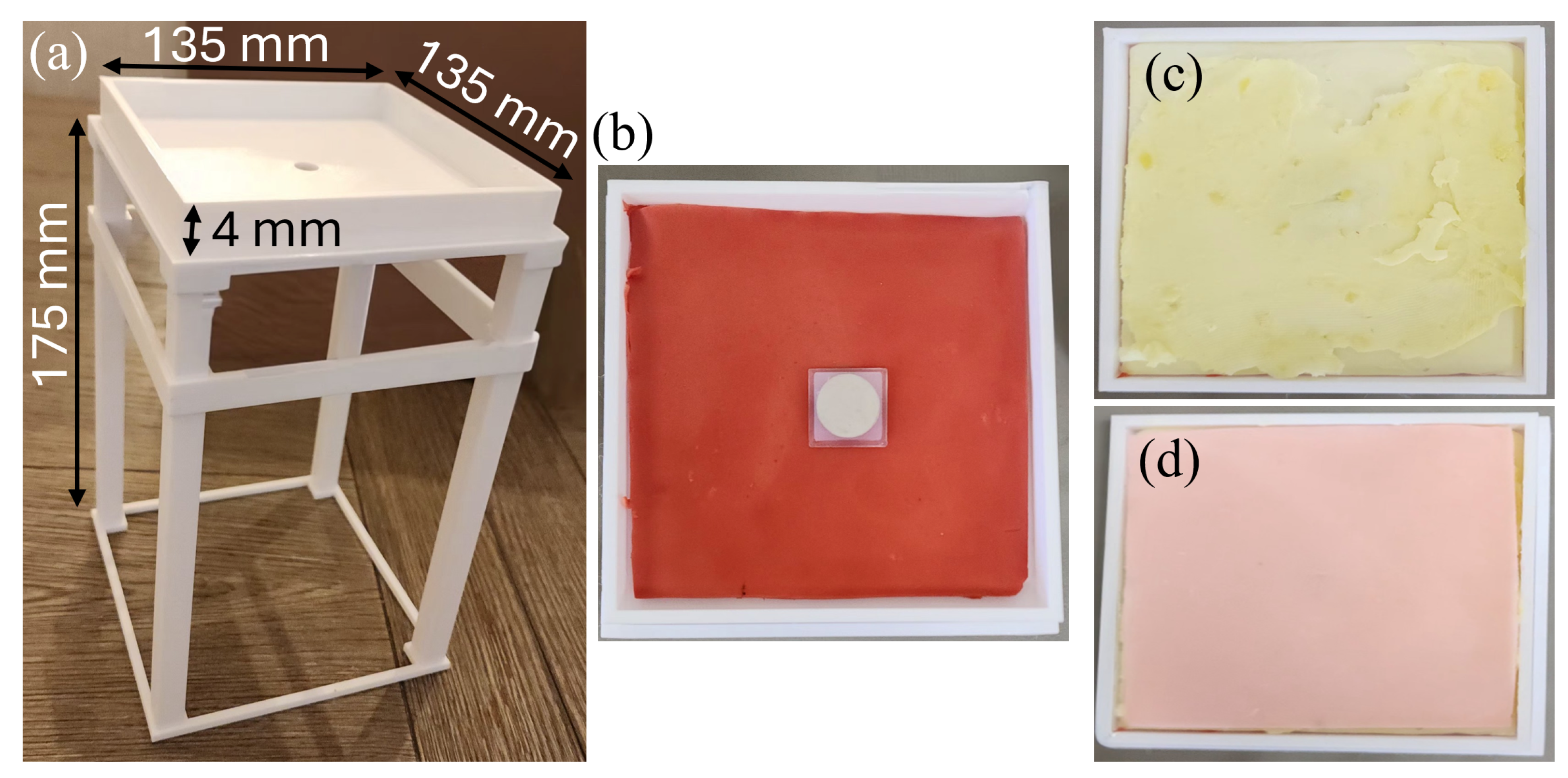
As shown in Figure 7a, a 3D-printed holding fixture was fabricated to provide adequate clearance for the SMA cable while securing the phantom tissues and implantable antenna for measurement. The top container is removable and features a central hole for easy access to the SMA connector. The phantom tissues are assembled by placing the muscle phantom inside the container, and then centering the implantable antenna on top of the muscle phantom by threading the SMA connector through the center hole (Figure 7b). Afterward, the adipose phantom is placed over the implantable antenna and muscle phantom (Figure 7c). Finally, the skin phantom is placed over the adipose phantom (Figure 7d).
Figure 7.
Fabricated holding apparatus and staggered phantom: (a) holding apparatus, (b) implantable antenna and muscle phantom (top view), (c) staggered adipose phantom (top view), and (d) staggered skin phantom (top view).
2.4. Model and Simulation
2.4.1. PSO Algorithm and Ansys HFSS
PSO is a population-based metaheuristic optimization method inspired by collective intelligence in swarms, in which each particle represents a candidate solution and updates its position based on its individual experience and group knowledge. PSO is well suited to iterative and real-time optimization, making it a favorable choice for antenna designers due to its simple implementation and rapid convergence [25]. Antenna designers for IMDs face a unique challenge due to the operating environment (e.g., implantation depth, antenna enclosure, tissue dielectric properties, and varying tissue thicknesses). Modeling and simulation of implantable antennas require substantial computational resources to account for the complex operating environment. Tunable antenna topologies provide designers with the flexibility to make subtle adjustments to reconfigure the antenna for a desirable operating frequency, thereby improving the antenna’s performance with respect to parameters such as bandwidth, gain, impedance, and return loss. The process of tuning an implantable antenna can be time-consuming, requiring downtime between simulations to manually adjust parameters using intuition.
Therefore, the present work aims to optimize the design of the serpentine implantable antenna using an open-source PSO algorithm. Table 5 provides a list of parameters for the PSO algorithm. The PSO algorithm is developed in Python and interfaces automatically with the Ansys HFSS model and simulation software, reducing the downtime between simulations. Although there are many antenna performance metrics to consider, we have selected as the key parameter for optimization. Antenna designers consider the acceptable range for return loss as ( ≥ −10 dB), which indicates minimal signal reflection and mismatch within the operational environment. The PSO algorithm employs Ansys HFSS as a solver for and thereby assigns an objective value to each particle. Each particle represents a unique combination of feed port and shorting pin locations (, , , and ) and iteratively updates its position based on individual and group experience to converge to an optimal antenna configuration.
Table 5.
PSO algorithm parameters.
A balance between population size and the objective function criteria is necessary to allow the PSO algorithm to efficiently solve for the optimal design. A small swarm population would yield limited coverage of the search space and require more iterations to ensure convergence, whereas a larger swarm population would converge more quickly and require fewer iterations. After running hundreds of simulations, we selected a swarm size of 25 particles and an objective function of ( ≥ −30 dB), which provides an effective balance among exploration, convergence, and metaheuristic search for the optimal configuration. Unlike many optimization methods that aim to search for the global maximum, our work leverages the PSO key advantage of rapid convergence and real-time optimization. The parameters for the individual influence and group influence are assigned random percentage values between 0% and 100%, whereas the parameters for the weight coefficient are assigned random percentage values between 50% and 100%. The exploitation constant and exploration constant incrementally increase after each iteration, emphasizing convergence while saving computational resources and time.
A 4D particle is conceptually difficult to visualize. The PSO generates real-time images for the objective value and function. The sections below discuss the algorithm implementation, the graphics generated for the particle’s objective values, and the calculated 4D plots for the objective function.
2.4.2. PSO Algorithm Implementation
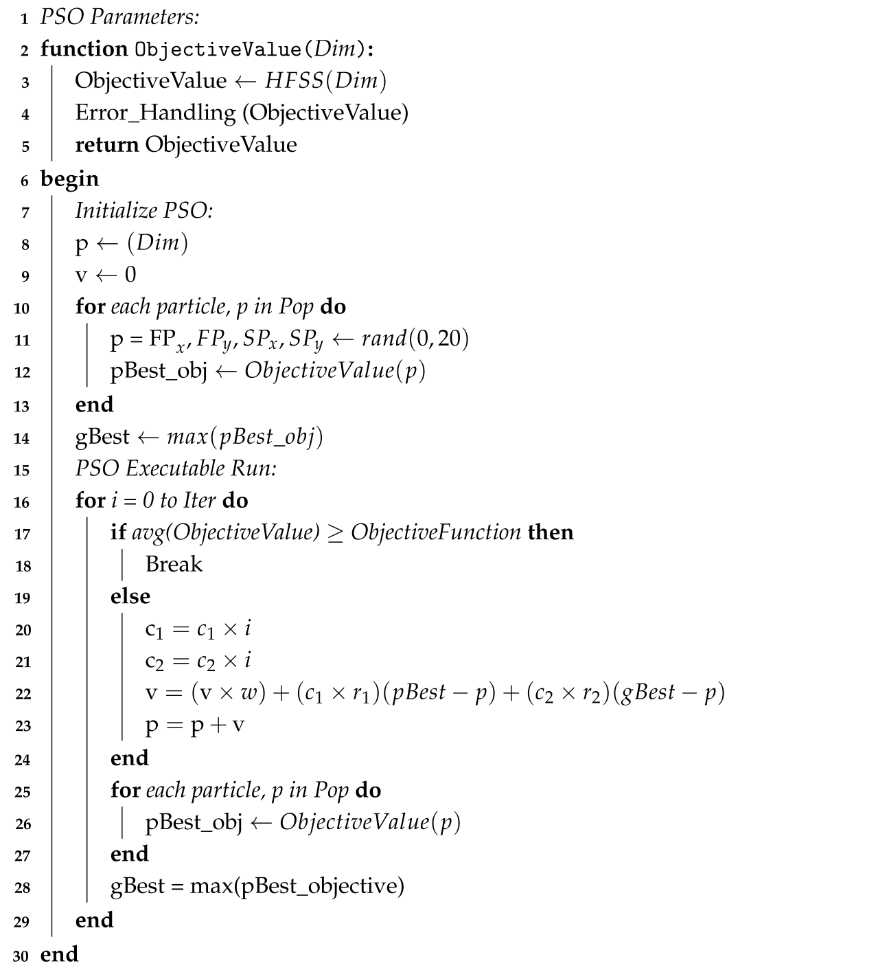
The following pseudocode provides a high-level representation of the logic implemented in the developed PSO algorithm. We modified a standard PSO algorithm to scholastically search for the optimal solution and to evaluate the objective function of a 4D particle. The mathematical expressions used a PSO algorithm, as shown in Equations (2)–(5). The annotation and represent a particle location and its velocity. Meanwhile, the superscript i and variable t denote the current position and iteration, respectively [26]. Furthermore, x and y represent the feed port and shorting pin, respectively.
As indicated in Equations (2) and (3), we initialize the PSO algorithm with each particle, p, by setting the velocity to zero and storing a random four-dimensional array positional value in correspondence with , , , and . The search space for , , , and are bounded between 0 and 20, expanding beyond the 19 mm substrate diameter by 1 mm. Ansys HFSS is deployed to evaluate the particle, producing an and assigning the objective function value. The gBest is then calculated by locating the particle with the highest objective value.
Lastly, the algorithm executes the iteration by verifying whether the objective function have been satisfied. If the objective function conditions has been met, the program ends; otherwise, the algorithm continues to execute Equations (4) and (5) by updating the particle’s new position, which is influenced by its current position, velocity, and the swarm’s best position [27].
2.4.3. Objective Function and 4D Plots
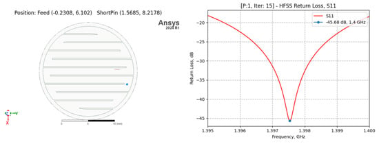
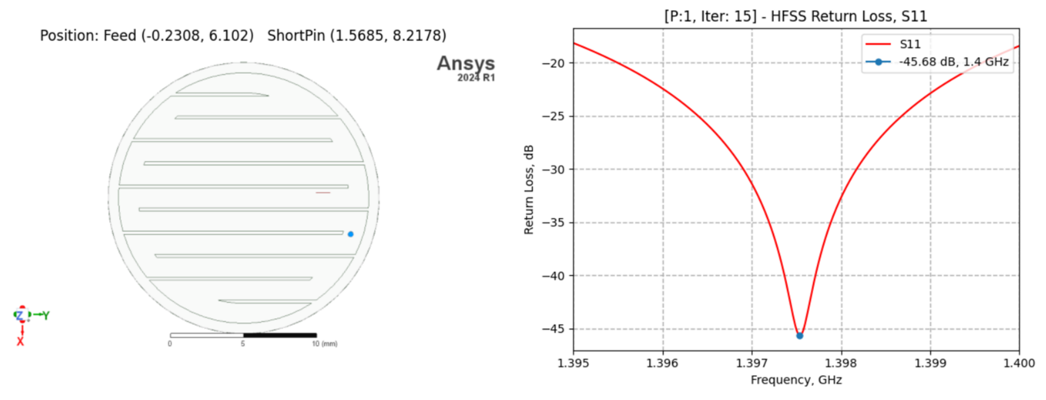
The PSO algorithm generates graphics for each evaluated particle. Figure 8 provides an example of the interaction between the PSO algorithm and Ansys HFSS. The algorithm extracts data from Ansys HFSS to create a summary report for each calculated objective value. The summary report includes a graphical image showing the feed port (, ), represented in a red line within the left image. Additionally, the shorting pin (, ) is represented by blue dots in the left image. The graphical image also provides a return loss plot with the simulated of −45.68 dB at 1.4 GHz presented in the right image. These graphics serve as historical records that enable the antenna designer to assess trends and select an optimal design that balances manufacturability and return loss. As expressed in Algorithm 1 lines 2–5, the algorithm provides a four-dimensional particle consisting of , , , and as a batch script for Ansys HFSS to execute. The batch script includes IronPython script instructions for running the simulation, calculating and exporting the plot, and exporting an image of the simulation run. The algorithm searches for the maximum value between 1.395 GHz and 1.400 GHz, and then allocates the data as the objective value for the specific particle and iteration (P:1, Iteration: 15).
Figure 8.
Particle 1, Iteration 15-PSO objective value summary report, feed port and shorting pin positions (left image), plot (right image).
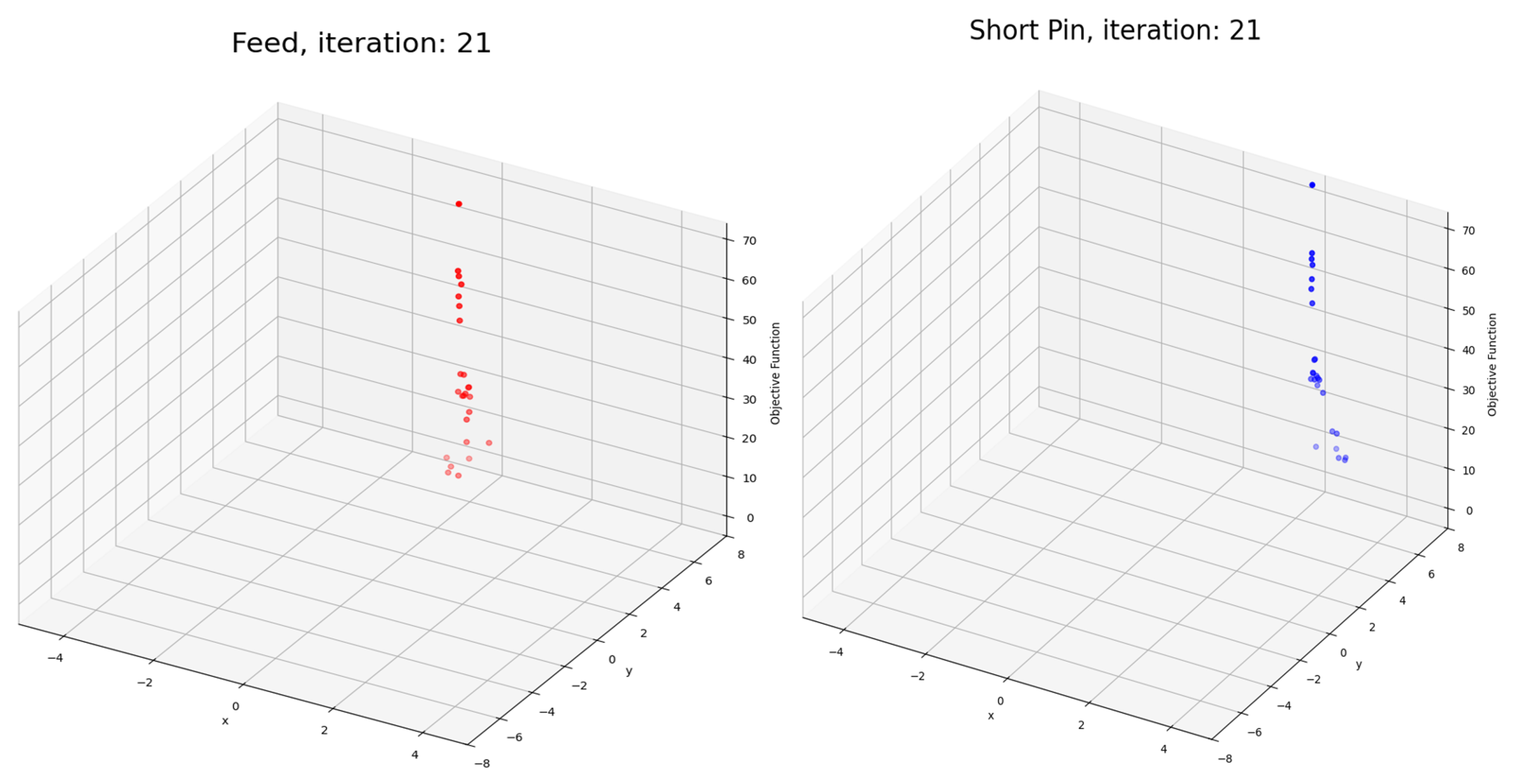
The 4D particles are complex to visualize; the particles for the feed port and shorting pin are separated into two 3D plots. As shown in Figure 9, the algorithm plotted 25 particles for the feed port (left image) and 25 particles for the shorting pin (right image) at the 21st iteration. This example displays valuable information such as the x and y positions (x and y axes) as well as the calculated objective value (z axis) for each particle. As expressed in Algorithm 1 line 17, the algorithm averages the objective value, and then verifies conditions for the objective function.
Figure 9.
PSO objective function with 25 particles at 21st iteration: feed port (left image) and shorting pin position (right image).
| Algorithm 1: PSO Algorithm Interface with HFSS |
 |
As shown in Figure 9, the objective criteria have been met, halting the execution after the 21st iteration. Even though the PSO algorithm has discovered particles with values between −50 dB and −70 dB, we have selected particle 1 from iteration 15 (Figure 8) for its ease of manufacturing and adequate . The PSO algorithm optimized the normalized (x, y) positions for the feed port at (−0.23, 6.10) and the shorting pin at (1.57, 8.22), resulting in a fitness value that yields an of −45.68 dB at 1.4 GHz. The translated coordinate points relative to the center are feed point (5.59 mm, 0.37 mm) and shorting pin (7.59 mm, −2.60 mm). Presented in Table 6 are the hardware specification, allocated hardware resources for HFSS, completed number of Ansys HFSS simulations, and completed run time.
Table 6.
Hardware specification and run time.
2.4.4. Current Distribution, Antenna Gain Pattern, and SAR
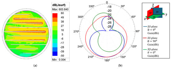
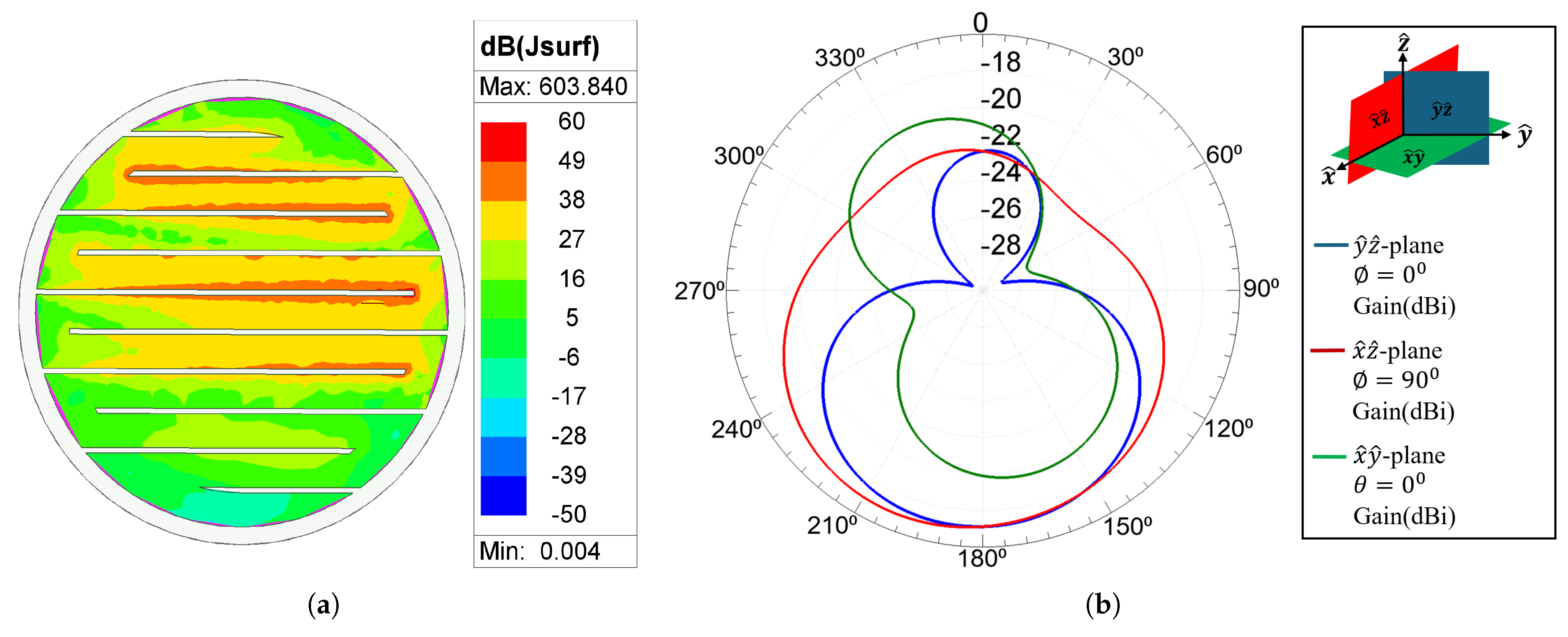
The simulated current distribution (Figure 10a) shows the majority of electron flows near the feed port and slots, while the shorting pin shunts some of the current flow near the bottom of the antenna. Furthermore, the antenna pattern (Figure 10b) provides the antenna gain at various azimuth, , and elevation, , yielding a simulated gain of −22.36 dBi.
Figure 10.
Implantable antenna: (a) current distribution and (b) gain radiation pattern.
The mandatory limits for Specific Absorption Rate (SAR) are established by the Federal Communications Commission (FCC) and the International Commission on Non-Ionizing Radiation Protection (ICNIRP), specifying the maximum limits of 1.6 (W/kg) averaged over 1 g of tissue and 2 (W/kg) averaged over 10 g of tissue. SAR is calculated using Equation (6), in which represents tissue conductivity, E denotes electric field intensity, and indicates the mass density of the tissue [25].
Table 7 summarizes the SAR parameters used to model human tissue as three distinct layers (skin, adipose, and muscle), resulting in an overall size of 127 mm × 127 mm × 14 mm. The mass density and frequency-dependent dielectric properties at 1.4 GHz were assigned to each tissue layer within Ansys HFSS.
Table 7.
SAR parameters at 1.4 GHz [25,28].
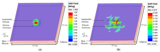
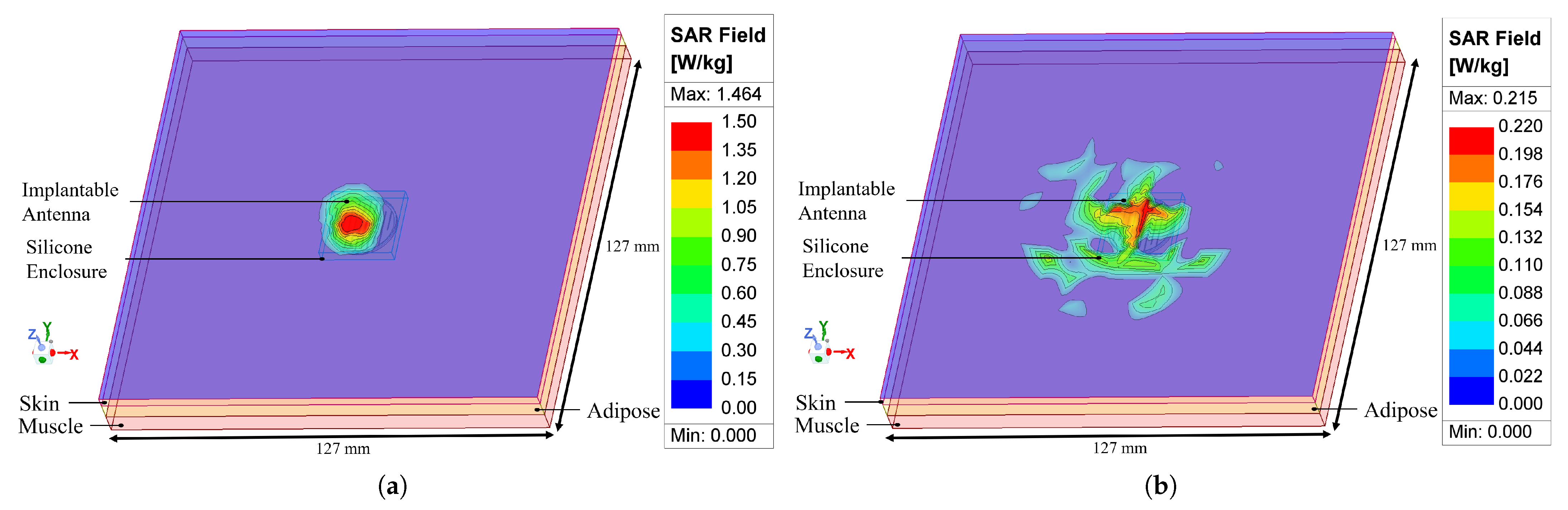
As shown in Figure 11, the antenna is implanted 7 mm within the subcutaneous layer, measured from the skin surface to the bottom of the enclosure. Simulations were performed in Ansys HFSS to evaluate the maximum SAR at 1.4 GHz with a default input power of 1 W. Figure 11a shows a maximum SAR value of 1.464 (W/kg), while Figure 11b shows a maximum SAR of 0.215 (W/kg). These results indicate that the proposed antenna complies with the FCC and ICNIRP exposure limits and is therefore suitable for implantable applications. An input power of 1.093 W and 9.302 W is necessary to achieve the FCC 1.6 (W/kg) and ICNIRP (2 W/kg) limits, respectively.
Figure 11.
Implantable antenna: (a) averaged SAR over 1 g of tissue and (b) averaged SAR over 10 g of tissue.
3. Measurements and Results
3.1. Test Setup
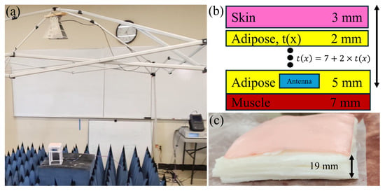
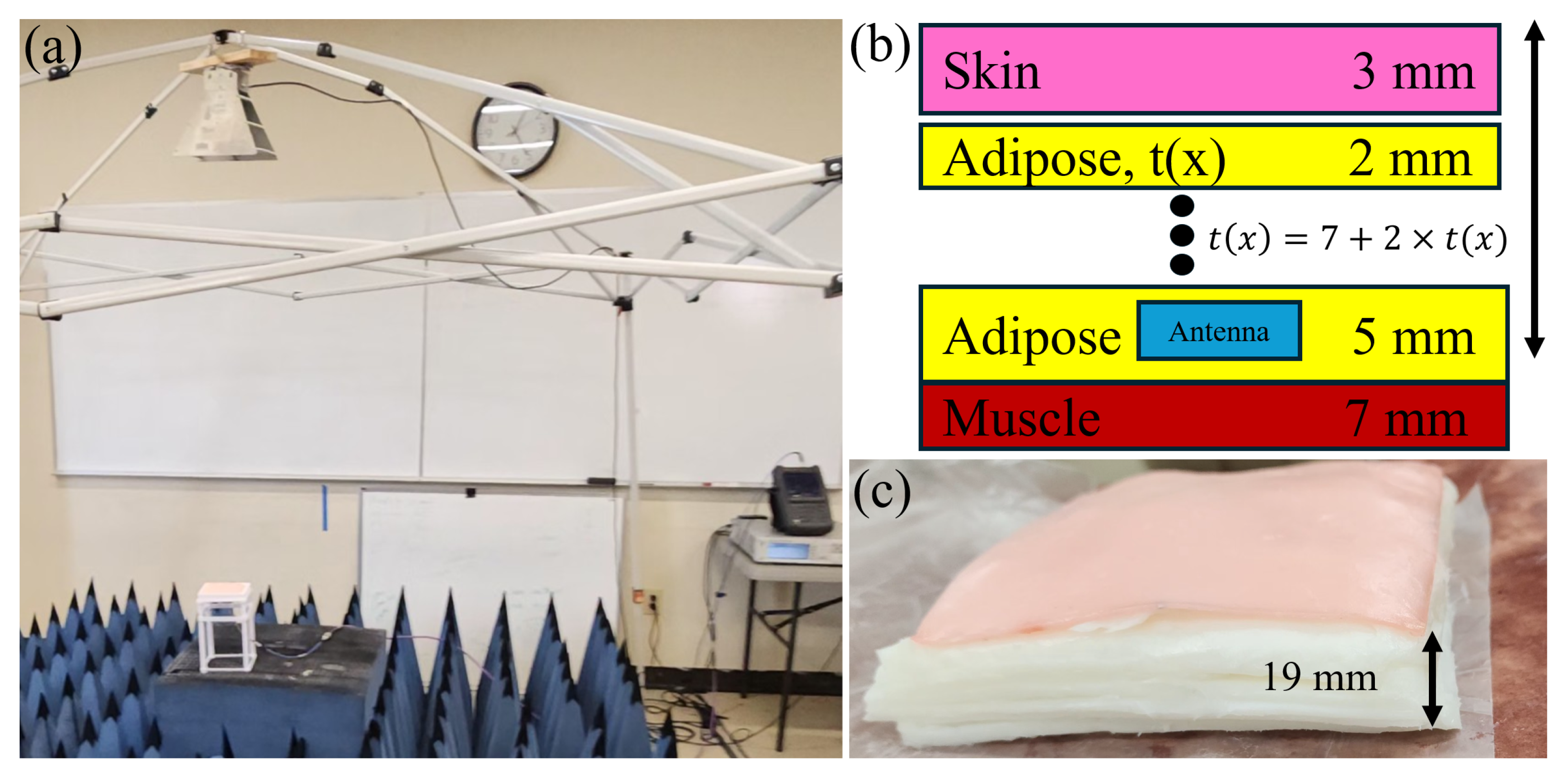
A vertical test setup was constructed to evaluate the antennas’ performance (Figure 12a). A custom test setup is necessary for this experiment since the gelatin phantoms could not be mounted vertically in the anechoic chamber. RF foam absorbers were employed to mitigate destructive scattering, and instrumentation, including an Agilent RF signal generator N5183B and a Keysight Field Fox vector network analyzer N9917A (VNA), was used to measure the gain, the return loss of implantable antenna ()/elliptical antenna (), and the insertion loss () between the two antennas. The phantom gels and adipose substitute (frozen butter and lard) were allowed to rest in the refrigerator and freezer for at least 24 h, respectively. Measurements using phantom gels were limited to 5 min to ensure that the gels remained cold to preserve their dielectric properties. Frozen lard was mass-produced in thin molds, with more than 30 samples available, thereby reducing overall measurement time. Measurements with frozen lard were limited to 2 min to ensure that the material remained fully frozen, preserving dielectric properties’ consistency.
Figure 12.
Test setup: (a) vertical test configuration, (b) adipose phantom layering, and (c) seven layers of adipose phantom.
As shown in Figure 12b, a 2 mm thick adipose phantom layer was staggered for each measurement to replicate various skin sites and body compositions. A total of seven layers of adipose phantom (17 mm thick) were staggered (Figure 12c), resulting in an implantation measurement depth between 7 mm and 19 mm.
3.2. Implantable Antenna Return Loss
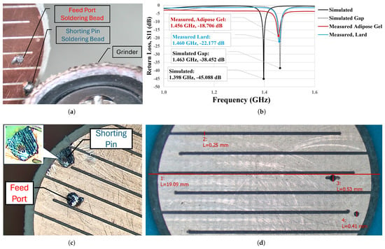
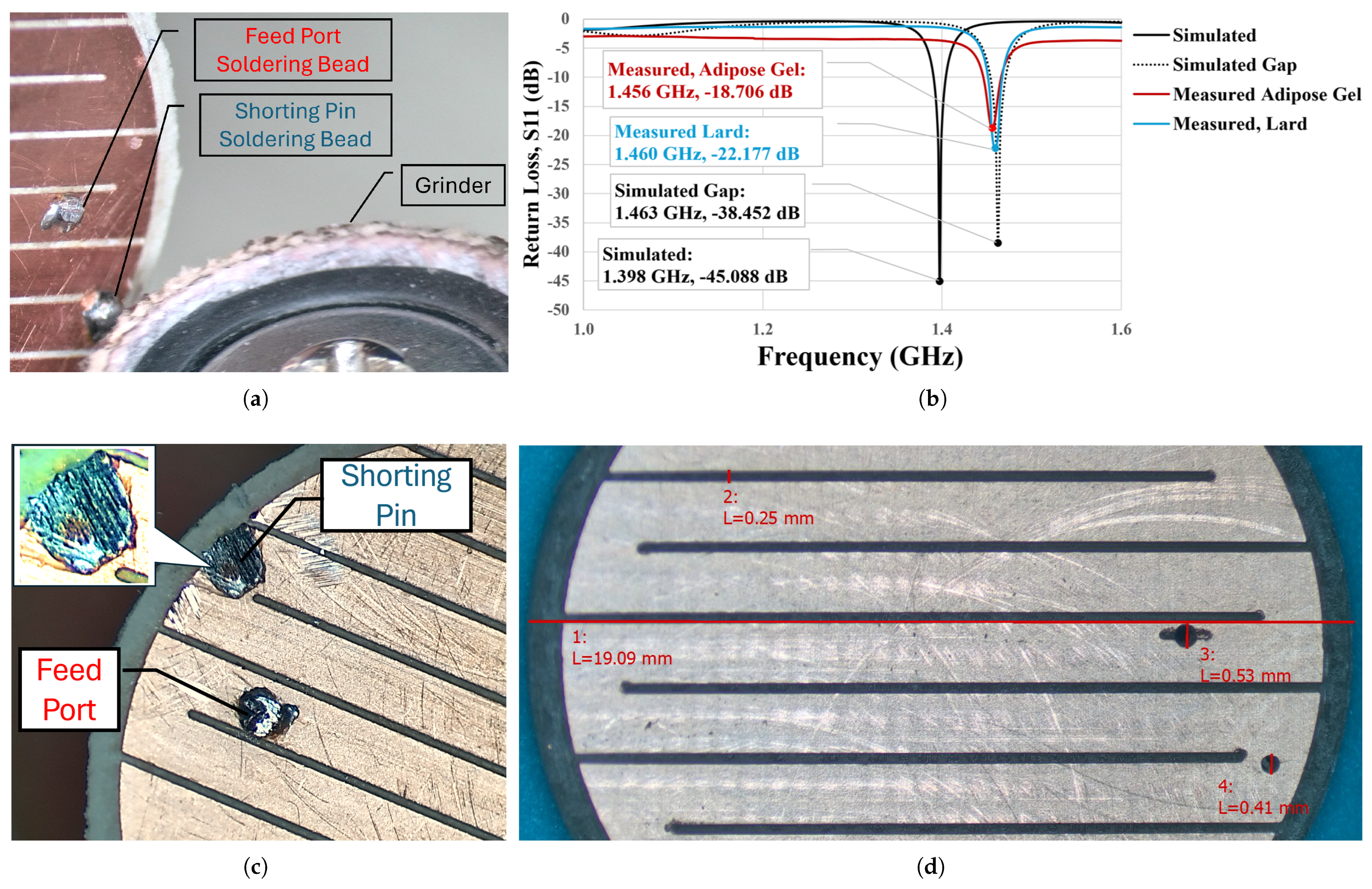
Using the signal generator, Keysight Field Fox VNA, and test setup (Figure 12a), the gain and were measured via in vitro testing with phantom tissues. The measured antenna gain yielded −24.40 dBi, which is relatively close to the simulated gain of −22.36 dBi (Figure 10b). As shown in Figure 13b, was measured and plotted. The simulated data show an of −45.09 dB at 1.398 GHz (solid black line), whereas the measured data points yielded −18.706 dB at 1.456 GHz via adipose tissue-mimicking gel (red solid line) and −22.177 dB at 1.460 GHz via frozen lard (blue solid line). Due to the relatively small and compact size of the antenna, the discrepancy between simulation and measurement could be a result of human error during manufacturing, particularly when working under a high-power microscope.
Figure 13.
Implantable antenna: (a) elevated soldering bead captured from high power microscope; (b) return loss (): simulation, simulated gap, measured adipose tissue-mimicking gel and frozen lard; (c) smoothed soldering beads for feed port and shorting pin; and (d) calibrated scaled measurements using microscope software (S-Eye v2.0).
By observation, a frequency shift of at least 150 MHz and an difference of approximately 23 dB were noticeable between the simulation and measured data points. The discrepancy can be attributed to the soldering bead, which generated a gap between the substrate and superstrate. During implantable antenna manufacturing, the RG-316 coaxial center conductor and the shorting pin are inserted through the ground plane and soldered to the patch plane, thereby forming a solid connection. As shown in Figure 13a, these soldering connections created a solder bead on the patch plane, creating a gap between the substrate and the staggered superstrate. Although a Dremel tool was used to grind the soldering bead, a small gap was evident through measurement. In the Figure 13b simulated gap plot (dotted black line), an estimated gap of 0.025 mm, smaller than the thickness of human hair, was simulated between the substrate and superstrate, demonstrating the antenna’s sensitivity to the superstrate-induced gap. Figure 13c shows the filed solder beads for the shorting pin and feed port. The shorting pin was smoothed with a Dremel tool, resulting in a thin film of solder exposing a small area of solid copper. Because the RG-316 center conductor and solder share a similar color, the feed port height is difficult to discern visually; however, we estimate that the height of the filed soldering joints is approximately 0.025 mm. Figure 13d presents calibrated scaled measurements from the microscope software. Using L2 (slot width), L3 (diameter of the shorting pin), and L4 (diameter of the feed port) as references, the thin film solder joints are observed to be much smaller, supporting the 0.025 mm estimate. As a result, the differences in and the frequency shift between the ideal simulation, the simulated gap, and the experimental data points are attributed to the gap between the substrate and superstrate.
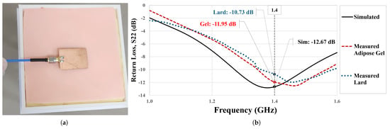
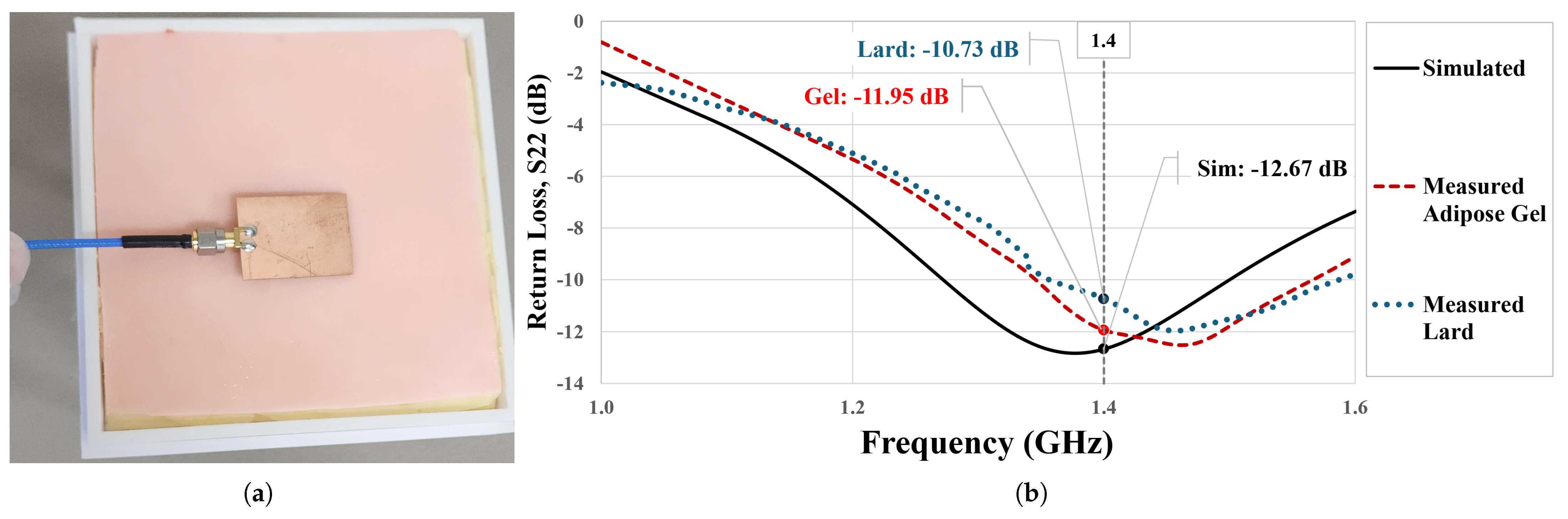
3.3. Elliptical Antenna Return Loss
The for the coupling elliptical antenna was measured using a Keysight Field Fox VNA. As shown in Figure 14a, the antenna was inverted and placed on top of staggering tissue phantoms. In Figure 14b, measurements via in vitro testing yielded −10.73 dB for frozen lard (dotted blue line) and −11.95 dB for adipose tissue-mimicking gel (dotted red line) at 1.4 GHz. By observation, the adipose tissue-mimicking gels closely match simulation, −12.67 dB at 1.4 GHz (solid black line). The differences can be attributed to the dielectric mismatch between the ideal and fabricated phantom tissues. Comparing between adipose mimicking gel and frozen lard, frozen lard yielded a similar profile with a difference of −1.22 dB at 1.4 GHz. As a result, frozen lard is a suitable substitute for a human adipose phantom with an operational bandwidth between 1.35 GHz and 1.6 GHz.
Figure 14.
Elliptical antenna: (a) in vitro testing with phantom tissues and (b) return loss (): simulation, measured adipose tissue-mimicking gel, and measured frozen lard.
3.4. Insertion Loss Between Elliptical and Implantable Antennas
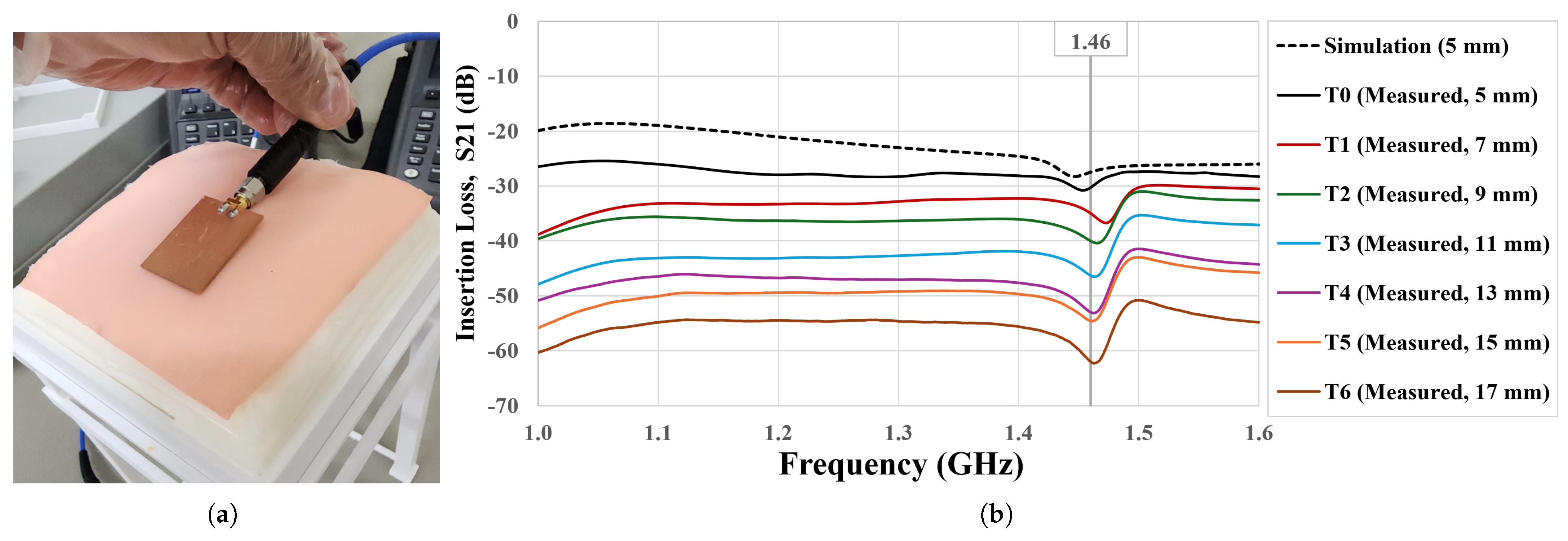
As shown in Figure 15a, measurements at 1.46 GHz were collected via in vitro testing with phantom tissues. An additional 2 mm thick adipose phantom (frozen lard) was inserted between the adipose and skin phantoms for each measurement, replicating various implantation depths and body compositions (Figure 10b). Before measurements were collected, the frozen lard and tissue-mimicking gels (skin and muscle phantoms) were allowed ample time to rest in the freezer and refrigerator, ensuring that the lard remained frozen solid and the gel remained cold to the touch. We selected a resonance frequency of 1.46 GHz to measure due to the manufacturing defect discovered in Figure 13. Figure 15b and Table 8 provide the plot and discrete data points for each measurement.
Figure 15.
Antenna coupling: (a) elliptical and implantable antennas’ in vitro testing with phantom tissues and (b) insertion loss () at various thicknesses.
Table 8.
Insertion loss at various implantation depth.
By observation, the plots for the simulation and measured adipose layer thickness zero, T0, are relatively close. Although there is a difference of −5.8 dB (Table 5) and a slight frequency shift (Figure 15b), the discrepancy can be attributed to the operational environment. The simulated plot encompasses the ideal dielectric properties of human tissues, whereas the measured T0 accounts for skin and muscle tissue-mimicking gels and adipose tissue substitute (frozen lard). The dielectric mismatch between phantom tissues (Figure 3a,d,e) presents the mismatch between measured and reference Cole–Cole plot, accounting for the differences between simulated and measured data points.
As shown in Table 8, the adipose phantom was staggered for each measurement, increasing the implantation depth by 2 mm, which inherently increased . T0 denotes the measurement at an initial implantation depth of 7 mm, whereas T1 through T6 denote measurements obtained by increasing the implantation depth in 2 mm increments. The differences between measurements were calculated to extract statistical data points. The calculated minimum (T5 and T4) and maximum (T6 − T5) differences between measurements are −1.56 dB (−1.56 dB = −54.56 dB − 53.00 dB) and −7.43 dB (−7.43 dB = −61.99 dB − 54.56 dB), respectively. Additionally, the calculated set mean is −5.29 dB between measurements, whereas the set median is −5.65 dB. Furthermore, the plot (Figure 15b) shows no significant frequency shifts between measurements.
The relationship between measurements corresponds to various skin sites and body compositions. For example, the upper arm and thigh of underweight and overweight adults correlate with the measurements collected from T0 to T4. Similarly, the abdomens of underweight and overweight adults correlate with measurements from T0 to T5 [18,19,20]. T6 measurements provide valuable data for people with a BMI > 25 (kg/m2).
Substantial evidence demonstrates that the approximate range for is between −5.29 dB and −5.65 dB for the implantable antenna radiating through 2 mm thick adipose tissue. We can estimate the received power between the two antennas using link budget terminology and formulae ( = + ). Assuming that the coupling antenna’s output power is 1 W, or 30 dBm, and the implantation depth is T0 (7 mm), the implantable antenna would receive 3.6 mW or 5.52 dBm (5.52 dBm = 30 dBm − 24.48 dB). Assuming the same conditions, but at the implantation depth of T1 (9 mm), the implantable antenna would receive 0.9 mW or −0.28 dBm (−0.28 dBm = 30 dBm − 30.28 dB). The value of beyond the thickness of T6 can be estimated using the average of −5.29 dB. However, for larger thicknesses, factors such as aggregated bandwidth and placement alignment must be considered, as they may increase the likelihood of IMD-induced detuning.
Although the implantable antenna design optimized through PSO demonstrated adequate results for various adipose thicknesses, the insertion loss between antennas can be improved by increasing the output power. Additionally, improving the design of the coupling antenna can also increase the link margin between antennas.
4. Conclusions
In this study, we introduce a tunable serpentine implantable antenna design optimized using an open-source PSO algorithm. Our work presents the design, simulation, and fabrication of the implantable and mutually coupled antennas. This design was verified through simulation, fabrication, and in vitro testing using phantom tissues with antenna performance evaluated for gain, , , and . We discuss the PSO process, pseudocode, 4D plots, and integration with simulation software, Ansys HFSS. Additionally, food products such as frozen salted butter and lard were substituted for adipose tissue-mimicking gels to evaluate the effects of implantable depth, as these materials can be fabricated into thin sheets with minimal cracking compared with conventional gels.
Our work presents several novel contributions: (1) an implantable antenna design with adjustable parameters that can be tailored to various skin sites, resonant frequencies, and implantation depths; (2) evaluating antenna performance at various implantation depths using adipose phantom substitutes to address the variability between skin sites and body compositions across people; and (3) applying an open-source modified PSO algorithm to optimize the implantable antenna design using dynamic exploration and exploitation constants and generate multidimensional plots. The parameters for the PSO are a population of 25 particles with 4 dimensions, 30 iterations, and an objective function of −30 dB. The objective function was satisfied at the 21st iteration, demonstrating a practical method to optimize antennas for biomedical applications.
Experimental data obtained through in vitro testing via phantom tissues validated the antenna design. Components of the operational environment, comprising tissue-mimicking gels, silicone rubber, lard, and salted butter, were fabricated and characterized to emulate their respective ideal electrical properties. Using tissue-mimicking gels, the antenna gain was measured, yielding −24.40 dBi, which is relatively close to the simulated value of −22.36 dBi. Furthermore, the for simulation is −45.088 dB at 1.398 GHz, and the simulated gap is −38.452 dB at 1.463 GHz, demonstrating that the implantable antenna design is affected by the superstrate-induced gap caused by the solder bead.
Measured and results demonstrate that frozen lard is an effective material for human adipose phantom, closely mimicking the dielectric properties of human adipose tissue. The measured using adipose gel is −18.706 dB at 1.456 GHz, while the measured with lard is −22.177 dB at 1.460 GHz, indicating minimal frequency shift and return loss with the implantable antenna. The at 1.4 GHz for simulation is −12.67 dB, compared with −11.95 dB for adipose gel, and −10.73 dB for frozen lard, confirming minimal return loss with the elliptical antenna. Despite these advantages, frozen lard has limitations, including poor conformability and temperature sensitivity. It must remain frozen during testing, whereas tissue-mimicking gel is semi-solid, which conforms well to flexible surfaces, and is less temperature sensitive.
Seven measurements were made to study the effects of implantation depth across different skin sites and body compositions. At T0 (7 mm implantation depth), a −5.8 dB difference in was observed between simulation and measurement, consistent with expected discrepancies from the mismatches between the Cole–Cole model for the ideal tissue properties and manufactured tissue-mimicking gels with frozen lard. Across all seven measurements, the calculated average is −5.29 dB, corresponding to an estimated insertion loss per 2 mm of adipose thickness. The initial measurements at T0 replicated the skin sites for the upper arm, abdomen, and thigh for underweight adults (BMI < 17–19 kg/m2). Measurements from T0 and T4 correspond to the upper arm and thigh, while measurements between T0 and T5 correspond to the abdomen of averaged underweight (BMI < 17 kg/m2) and overweight adults (BMI > 25 kg/m2) [18,19,20].
Although discrepancies were observed between simulated and measured data points (Figure 13), a high-precision soldering manufacturer can offer laser or robotic soldering, minimizing the gap between the substrate and superstrate, thereby improving the frequency shift and increasing the return loss. Alternatively, solder paste and controlled heat can minimize the soldering bead. Although hand soldering using a high-power microscope is challenging for devices as small as a U.S. dime, the instrumentation is suitable for experimentation, favorable due to its cost, accessibility, and ease of use.
In conclusion, this study fills a knowledge gap not discussed in other studies, like antenna performance at various skin sites, body compositions, and implantation depths. Compared with other studies, this paper focuses on an approach to optimize an implantable antenna using an PSO algorithm and validates the antenna design via simulation and in vitro testing, while addressing suitable substitute materials for adipose phantom. The PSO algorithm is open-source and generates multidimensional plots of the objective function and graphics for the objective value and function. These graphics provide a historical record for identifying optimization trends and selecting an optimal design that balances return loss and manufacturability. In addition to the feed port and shorting pin, other tunable design variables can be used to increase the dimensionality of the PSO particle. Future work can be extended to dual-band resonance frequencies by optimizing other variables, such as N-turns and the diameter of the shorting pin.
5. Data and Code Availability
The related code and synthetic data used for antenna optimization can be found in the GitHub repository (https://github.com/mpn21/An-Implantable-Antenna-Design-Optimized-Through-an-AI-ML-PSO-Algorithm.git, accessed on 5 November 2025).
Author Contributions
Conceptualization, M.P.N. and R.B.G.; methodology, M.P.N.; software, M.P.N.; validation, M.P.N. and R.B.G.; formal analysis, M.P.N.; investigation, M.P.N.; resources, R.B.G.; data curation, M.P.N.; writing—original draft preparation, M.P.N.; writing—review and editing, M.P.N., L.L., and M.J.S.; visualization, M.P.N.; supervision, R.B.G.; project administration, M.P.N.; funding acquisition, M.P.N. All authors have read and agreed to the published version of the manuscript.
Funding
This research received no external funding.
Institutional Review Board Statement
Not applicable.
Informed Consent Statement
Not applicable.
Data Availability Statement
The raw data supporting the results and conclusions of this article will be made available by the authors on request.
Acknowledgments
We would like to acknowledge Erdem Topsakal at Virginia Commonwealth University for providing the tissue-mimicking gels and Junming Diao at Mississippi State University for providing access to the test equipment for this research.
Conflicts of Interest
The author declares no conflicts of interest.
Abbreviations
The following abbreviations are used in this manuscript:
| ANNs | artificial neural networks |
| Ansys HFSS | Ansys High Frequency Structure Simulator |
| BMI | body mass index |
| CGM | continuous glucose monitoring |
| CRT-D | cardiac resynchronization therapy defibrillator |
| DBS | deep brain stimulation |
| DoFs | Degrees of Freedom |
| DT | decision tree |
| FCC | Federal Communications Commission |
| FDA | Food and Drug Administration |
| ICD | implantable cardioverter defibrillator |
| ICNIRP | International Commission on Non-Ionizing Radiation Protection |
| IMD | implantable medical device |
| ML | machine learning |
| PSO | particle swarm optimization |
| SAR | Specific Absorption Rate |
| SJM | St. Jude Medical |
| SVR | support vector regression |
| WMTS | wireless medical telemetry service |
| VNA | vector network analyzer |
References
- Bhargava, K.; Arora, V.; Jaswal, A.; Vora, A. Premature battery depletion with St. Jude Medical ICD and CRT-D devices: Indian Heart Rhythm Society Guidelines for physicians. Indian Heart J. 2019, 71, 12–14. [Google Scholar] [CrossRef] [Scilit] [PubMed]
- U.S. Food and Drug Administration Center for Devices and Radiological Health. Permarket Approval (PMA) P960009; U.S. Food and Drug Administration Center for Devices and Radiological Health: Silver Spring, MD, USA, 2018.
- U.S. Food and Drug Administration Center for Drug Evaluation and Research. Premarket Approval (PMA) P160048; U.S. Food and Drug Administration Center for Devices and Radiological Health: Silver Spring, MD, USA, 2022.
- Zada, M.; Yoo, H. A Miniaturized Triple-Band Implantable Antenna System for Bio-Telemetry Applications. IEEE Trans. Antennas Propag. 2018, 66, 7378–7382. [Google Scholar] [CrossRef] [Scilit]
- Green, R.B.; Hays, M.; Mangino, M.; Topsakal, E. An Anatomical Model for the Simulation and Development of Subcutaneous Implantable Wireless Devices. IEEE Trans. Antennas Propag. 2020, 68, 7170–7178. [Google Scholar] [CrossRef] [Scilit]
- Liu, C.; Guo, Y.X.; Sun, H.; Xiao, S. Design and Safety Considerations of an Implantable Rectenna for Far-Field Wireless Power Transfer. IEEE Trans. Antennas Propag. 2014, 62, 5798–5806. [Google Scholar] [CrossRef] [Scilit]
- Hood, A.Z.; Topsakal, E. Particle swarm optimization for dual-band implantable antennas. In Proceedings of the 2007 IEEE Antennas and Propagation Society International Symposium, Honolulu, HI, USA, 9–15 June 2007; pp. 3209–3212. [Google Scholar] [CrossRef] [Scilit]
- Shah, S.A.A.; Yoo, H. Radiative Near-Field Wireless Power Transfer to Scalp-Implantable Biotelemetric Device. IEEE Trans. Microw. Theory Tech. 2020, 68, 2944–2953. [Google Scholar] [CrossRef] [Scilit]
- Karacolak, T.; Hood, A.Z.; Topsakal, E. Design of a Dual-Band Implantable Antenna and Development of Skin Mimicking Gels for Continuous Glucose Monitoring. IEEE Trans. Microw. Theory Tech. 2008, 56, 1001–1008. [Google Scholar] [CrossRef] [Scilit]
- Karacolak, T.; Topsakal, E. Electrical properties of nude rat skin and design of implantable antennas for wireless data telemetry. In Proceedings of the 2008 IEEE MTT-S International Microwave Symposium Digest, Atlanta, GA, USA, 15–20 June 2008; pp. 907–910. [Google Scholar] [CrossRef] [Scilit]
- Tung, L.V.; Seo, C. A Miniaturized Implantable Antenna for Wireless Power Transfer and Communication in Biomedical Applications. J. Electromagn. Eng. Sci. 2022, 22, 440–446. [Google Scholar] [CrossRef] [Scilit]
- Rasool Khan, U.; Sheikh, J.A.; Junaid, A.; Ashraf, S.; Balkhi, A.A. A machine learning driven computationally efficient horse shoe shaped antenna design for internet of medical things. PLoS ONE 2025, 20, e0305203. [Google Scholar] [CrossRef] [Scilit] [PubMed]
- Khan, S.R.; Pavuluri, S.K.; Cummins, G.; Desmulliez, M.P.Y. Wireless Power Transfer Techniques for Implantable Medical Devices: A Review. Sensors 2020, 20, 3487. [Google Scholar] [CrossRef] [Scilit] [PubMed]
- Karacolak, T.; Cooper, R.; Butler, J.; Fisher, S.; Topsakal, E. In Vivo Verification of Implantable Antennas Using Rats as Model Animals. IEEE Antennas Wirel. Propag. Lett. 2010, 9, 334–337. [Google Scholar] [CrossRef] [Scilit]
- Basir, A.; Yoo, H. Efficient Wireless Power Transfer System with a Miniaturized Quad-Band Implantable Antenna for Deep-Body Multitasking Implants. IEEE Trans. Microw. Theory Tech. 2020, 68, 1943–1953. [Google Scholar] [CrossRef] [Scilit]
- Wang, M.; Liu, H.; Zhang, P.; Zhang, X.; Yang, H.; Zhou, G.; Li, L. Broadband Implantable Antenna for Wireless Power Transfer in Cardiac Pacemaker Applications. IEEE J. Electromagn. RF Microwaves Med. Biol. 2021, 5, 2–8. [Google Scholar] [CrossRef] [Scilit]
- Nguyen, M.P.; Green, R.B. Wearable E-Textile Antenna Design for Continuous Monitoring Systems. Textiles 2025, 5, 2. [Google Scholar] [CrossRef] [Scilit]
- Sim, K.H.; Hwang, M.S.; Kim, S.Y.; Lee, H.M.; Chang, J.Y.; Lee, M.K. The Appropriateness of the Length of Insulin Needles Based on Determination of Skin and Subcutaneous Fat Thickness in the Abdomen and Upper Arm in Patients with Type 2 Diabetes. Diabetes Metab. J. 2014, 38, 120–133. [Google Scholar] [CrossRef] [Scilit] [PubMed]
- Jain, S.M.; Pandey, K.; Lahoti, A.; Rao, P.K. Evaluation of skin and subcutaneous tissue thickness at insulin injection sites in Indian, insulin naïve, type-2 diabetic adult population. Indian J. Endocrinol. Metab. 2013, 17, 864–870. [Google Scholar] [CrossRef] [Scilit] [PubMed]
- Gibney, M.A.; Arce, C.H.; Byron, K.J.; Hirsch, L.J. Skin and subcutaneous adipose layer thickness in adults with diabetes at sites used for insulin injections: Implications for needle length recommendations. Curr. Med. Res. Opin. 2010, 26, 1519–1530. [Google Scholar] [CrossRef] [Scilit] [PubMed]
- Gassmann, B. Electrical and dielectric properties of food materials. A bibliography and tabulated data. Zusammengestellt von M. Kent. 135 Seiten. Science and Technology Publishers, Hornchierch, Essex, England, 1987. Preis: 20.00 £. Food Nahr. 1988, 32, 356. [Google Scholar] [CrossRef] [Scilit]
- Dancsisin, M. Characterization of Tissue Mimicking Materials for Testing of Microwave Medical Devices. Master’s Thesis, Mississippi State University, Mississippi State, MS, USA, 2011. [Google Scholar]
- Gabriel, S.; Lau, R.W.; Gabriel, C. The dielectric properties of biological tissues: II. Measurements in the frequency range 10 Hz to 20 GHz. Phys. Med. Biol. 1996, 41, 2251. [Google Scholar] [CrossRef] [Scilit] [PubMed]
- Balanis, C.A. Antenna Theory: Analysis and Design, 4th ed.; John Wiley & Sons: Hoboken, NJ, USA, 2016. [Google Scholar]
- Reguig, M.; Belkheir, M.; Mokaddem, A.; Rouissat, M.; Ziani, D. AI Driven Design of High-Gain THz Antennas Using PBG Structures: Combining Evolutionary Algorithms and Machine Learning for Implantable Biomedical Systems. Biomed. Mater. Devices 2025. [Google Scholar] [CrossRef] [Scilit]
- Eberhart, R.C.; Shi, Y. Chapter three-Evolutionary computation concepts and paradigms. In Computational Intelligence; Eberhart, R.C., Shi, Y., Eds.; Morgan Kaufmann: Burlington, MA, USA, 2007; pp. 39–94. [Google Scholar] [CrossRef] [Scilit]
- Eberhart, R.C.; Shi, Y. Chapter four-Evolutionary computation implementations. In Computational Intelligence; Eberhart, R.C., Shi, Y., Eds.; Morgan Kaufmann: Burlington, MA, USA, 2007; pp. 95–143. [Google Scholar] [CrossRef] [Scilit]
- Gabriel, C.; Gabriel, S.; Corthout, E. The dielectric properties of biological tissues: I. Literature survey. Phys. Med. Biol. 1996, 41, 2231. [Google Scholar] [CrossRef] [Scilit] [PubMed]

Disclaimer/Publisher’s Note: The statements, opinions and data contained in all publications are solely those of the individual author(s) and contributor(s) and not of MDPI and/or the editor(s). MDPI and/or the editor(s) disclaim responsibility for any injury to people or property resulting from any ideas, methods, instructions or products referred to in the content. |
© 2026 by the authors. Licensee MDPI, Basel, Switzerland. This article is an open access article distributed under the terms and conditions of the Creative Commons Attribution (CC BY) license.