


Abstract
Although machine learning-based forecasting models often function as opaque black boxes, explainability methods provide the essential tools required to foster trust in deep learning systems, optimize computational resources, and enhance model accuracy. Motivated by this, we propose a model-agnostic, local explainability method specifically designed for forecasting tasks. Our approach employs a hierarchical structure that is generated iteratively. From the outset, a small number of “interpretable components” that decompose the input are considered. In the inductive step, the methodology enables analysts to examine the data in greater detail, allowing for a deeper exploration of specific subcomponents whenever a higher resolution is required. This framework inherently provides control over computational costs by tuning the branching factor. The resulting explainability tree shares certain, but not all, properties of the explainability values provided by the SHAP-LIME framework; in this regard, we present some theoretical results. Furthermore, numerical experiments provided evidence that explanation coherence is fundamentally maintained between both methods. We explored the utility of this methodology on a real-world short-term load forecasting LSTM encoder–decoder model.
1. Introduction
Machine learning-based forecasting models often act as black-box systems. Their inputs typically consist of tensors comprising historical features, known future covariates, and other predefined information; conversely, their outputs project multi-step-ahead sequences across specified forecasting horizons. Within this setting, we present a model-agnostic, post hoc, and inductive method inspired by the foundational principles of KernelSHAP [1,2,3]. Our approach allows analysts to consider interpretable sub-components down to the required level of precision, focusing on detailed close-ups only where the analysis deems it necessary.
A simple way to apply KernelSHAP to multivariate time-series models is to treat each temporal feature cell as an independent unit. However, this leads to a combinatorial explosion; although sampling methods avoid evaluating all coalitions, they still sacrifice precision or interpretability. Several methods have developed strategies to address the computational cost issue within the time-series framework. For classification tasks, TimeSHAP is an explainability method that extends KernelSHAP to the sequential domain [4]. A key component of this approach is a pruning method that significantly reduces the computational overhead by discarding older historical data. TimeSHAP assumes that temporally distant observations are less influential. However, this is not always the case; see a counterexample in [5] [Figure 1]. On the other hand, WindowSHAP introduces several variants, ranging from uniform time segmentation to an iterative refinement method that increases the resolution around significant attribution values [5]. Both methods rely on thresholds based on “small” Shapley values to guide subsequent operations, potentially hindering the adaptation of the algorithm from classification to forecasting, particularly when dealing with extended forecast horizons.
Finally, the SeqSHAP method incorporates subsequence-level explanations [6]—specifically through temporal partitions for each feature. This approach essentially constitutes a special case of the “close-up” concept introduced in this work. The authors did not consider the error between the sum of sequential contributions and the total contribution computed at the initial stage; thereby, a hierarchical structure is not necessarily guaranteed. Indeed, our approach resolves this inconsistency by correcting the error at each step.
In this work, we propose a methodology based on interpretable components, which can be iteratively refined through the forecaster’s knowledge using what we call “close-ups”. Each close-up assumes that some players are temporarily unavailable, which allows for a more detailed analysis. The proposed explainability model produces a tree whose nodes provide explanations at different levels of granularity. The hierarchical structure provides a clearer explainability narrative. Furthermore, we present a mathematically rigorous and empirical analysis of the relationship between our methodology and the traditional KernelSHAP approach. The advantages of our method include:
- Control of computational costs based on a maximum branching factor.
- Flexibility of application to specific contexts.
- Simple implementation, particularly in production forecasting cycles.
- Adaptability in the level of analysis.
- Explainability consistency across steps.
We present Table 1 to provide a concise comparative overview of the key characteristics of the aforementioned methods, for which we share several insights. The goal of these methods is to identify the relevant sections that determined the classification, thereby facilitating an expert analysis. Although it is possible to adapt these methods for forecasting, our approach, in contrast, integrates the expert into the system to explore and iteratively refine input variable concepts through close-ups, bypassing the simultaneous management of numerous input components lacking an interpretive narrative.
Table 1.
Comparative summary of similar model-agnostic and post hoc explainability approaches for time series.
The paper is structured as follows. Section 2 presents the general methodology and establishes several key properties of the proposed explainability vectors. Section 3 details the computation of these vectors and discusses the limitations of sampling for their estimation, alongside insights into the computational cost and the relationship between the hierarchical fitting error and global explainability properties equivalent to those of Shapley values. Section 4 evaluates the practical utility of this framework through a short-term energy demand forecasting case study using real-world data and a production model. Finally, concluding remarks are provided in Section 5, and all formal proofs are collected in Appendix A.
2. Explainability Trees
For a forecasting model f, we consider any trained model that takes as the input a finite sequence of time-feature matrices, e.g., , accepting different matrix sizes—for instance, matrices corresponding to historical variables, known future covariates, or other inputs consistent with the architecture—and outputs a time vector Y with the corresponding variable for future instances to be forecasted. By an interpretable decomposition of the input, we mean a partitioning of the input associated with semantic terms linked to an explanatory narrative. That is, an arbitrary split of X:
such that there are no overlaps between the parts and the concatenation of all of them, with respect to their original structure, is X itself. We refer to each as an interpretable component when it has a clear interpretation for forecasters, e.g., “weekends”, “the temperature in the past”, “the endogenous variable lagged by 3 days”, “holiday information given in advance”, or even “everything else”. If the structure of X is intricate, we can use “grouping” methods; for instance, we can decompose X into multivariate time-series groups where the dependence between variables within the same group is high, but very low between variables in different groups [7]. Alternatively, we can use time-series segmentation techniques to divide the time series into different semantic segments (see, e.g., [8]). Consequently, after this assisted decomposition, some degree of interpretability can be established for the resulting mutually disjoint groups.
The core idea of the proposed method is to apply an initial rule based on an interpretable decomposition of components. Upon evaluating the results, we proceed with an inductive rule that incorporates interpretable sub-components, allowing for a closer look at a specific component. This iterative process can be continued until there are enough elements to explain the model. For example, the interpretable component “weekends” can be split into subcomponents “Saturdays” and “Sundays”. The final result will be an initial bias ; the explainability vectors in ; and the tree-based links associated with the interpretable components and subcomponents. We refer to these elements as the explainability tree.
Let X be a fixed input and be the forecast over future time steps. We propose the following methodology:
- Initial rule.
- Start with a fixed initial interpretable decomposition . Compute according to the methodology described in Section 3. For every , set . We shall call the initial bias.
- Inductive rule.
- For some in the interpretable decomposition considered in the previous iteration, let be a subdecomposition of such that , where is the remainder of X. Compute and the columns of the matrix , , according to the methodology given in Section 3. For each , we set , where is a vector independent of k.
In each close-up, for each , we suppose that the estimate of has an uncertainty error representing a fraction of the total error: . In order to preserve the hierarchical structure, we set and . Consequently, the coefficients form a probability distribution. The principle of maximum entropy states that, when choosing a probability distribution for a system with incomplete information, the least biased choice is the one that maximizes entropy. Under conditions of complete ignorance or in the absence of prior information, the principle of maximum entropy dictates that all components are assumed to contribute equally to the total error [9] [Example 12.2.4]. Therefore, we set . The uniform distribution serves as a baseline distribution that can be adjusted when additional information about the system becomes available—for instance, if the errors are structurally related to the magnitude of the estimated individual contributions, a relation that cannot be generally assumed.
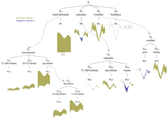
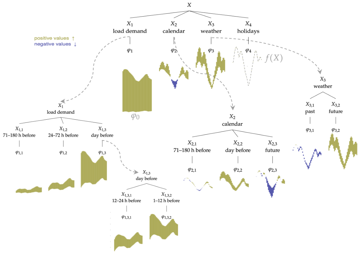
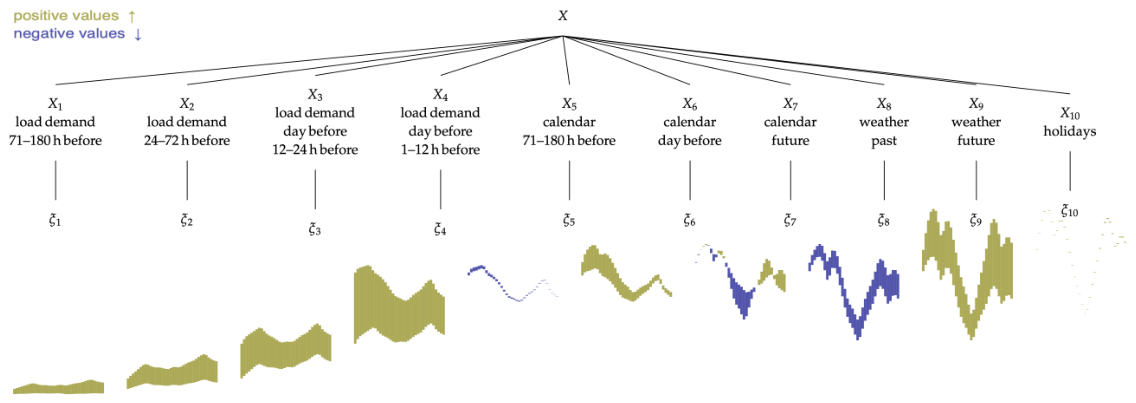
We can now formally associate a tree configuration with this inductive process. The initial decomposition generates a tree rooted at X with children for . In turn, each subsequent subdecomposition considered in the process generates new children with as their parent. If is computed for some , then becomes a child of for . Ultimately, the leaves of the tree, which can be relabeled as , are the final explainability vectors with respect to tree configuration . See Algorithm 1. An example of an explainability tree is shown in Figure 1.
| Algorithm 1 Explainability tree. |
|
Figure 1.
Explainability tree for 36 h ahead STLF to explain the inference of the load demand on a summer day, given the input X to an LSTM encoder–decoder model f. For each hour t, the positive values (green bars) of the explainability vectors increase the accumulated value starting from , while the negative values (blue bars) decrease it; the final total of the sum is the forecast . Each explainability vector can be decomposed into new vectors (gray arrows) that provide more precise explainability information.
The explainability tree satisfies the following consistency properties:
- 1.
- Breakdown contributions: .
- 2.
- Local symmetry: If the local marginal contribution of two interpretable components and sharing the same parent node is identical for every coalition , then .
- 3.
- Global efficiency: .
- 4.
- Global nullity with error: If the global marginal contribution of an interpretable component is null, then .
3. Estimation of Explainability Vectors
Let X be a fixed observation, and let be an initial interpretable decomposition or any further interpretable subdecomposition such that:
where is the remainder of X disjoint from . For the initial decomposition, there is no and is X. We want to adjust a linear explainability model acting on the absence/presence of the interpretable subcomponents with the remainder fixed, namely an affine map:
where is a matrix whose columns correspond to a vector associated with the interpretable subcomponent :
To fit , we generated a weighted pairwise dataset
with the weights given by , where is the number of nonzero entries and:
To estimate , we employed Algorithm 2 using a sample from a training set such that all elements within the sample share the same structure as X—specifically, possessing the same lookback window. Furthermore, the interpretable components must remain consistent across all elements of the sample in accordance with X. Following the framework of the KernelSHAP methodology, we considered the optimization problem . Let and be the n-dimensional zero and ones vectors, respectively. Note that . Consequently, and . The optimization problem can then be solved by embedding these constraints directly into the configuration of , minimizing over using standard weighted least squares solvers.
| Algorithm 2 Estimation of . |
|
Let be considered at any iteration in the inductive process such that , where may be nonexistent. For a fixed , the vectors are the Shapley values for the game —see Appendix A below:
In particular, if n is small, the values , can be calculated directly from the well-known Shapley value formula [10] [eq. 13].
Remark 1.
On the definition and estimation of : The conditional expectation is proposed instead of , which is typically used in the LIME framework [3], where maps binary values into the original input space. In that context, shares the same values as X, but contains “missing values” for the components not indicated by z. For instance, Bento et al. [4] handled missing values in their TimeSHAP methodology by replacing them with the sample mean of the corresponding features. A similar approach was considered by Jiang et al. [6] in their SeqSHAP method. In contrast, we adopted an approach analogous to that of Štrumbelj and Kononenko [1] to estimate feature contributions, aligned with the framework proposed by Lundberg and Lee for the well-known SHAP values [2]. This marginalization approach is also considered in the WindowSHAP methodology [5] within the context of time series. Notably, the estimation of is subject to the inherent limitations of SHAP values. Specifically, Algorithm 2 involves masked inputs that, despite being syntactically compatible with f, may lie out of distribution with respect to the training set. Actually, as Kumar et al. [11] pointed out, “f has never seen an example like this in training, and has therefore not learned much about this part of the feature space. Its predictions on this feature space are not necessarily relevant to the task of explaining an in-distribution”. Indeed, Slack et al. [12] presented a technique that effectively hides the biases of any given classifier by allowing an adversarial entity to construct arbitrary, desired LIME and SHAP explanations. Nevertheless, our approach can be used as a complementary tool in the training stage of the forecasting cycle. In particular, verifying the effectiveness of adjustments based on information provided by explainability models is a natural part of the forecaster design cycle, e.g., to corroborate whether the performance improves after making some decisions based on the proposed methodology.
Remark 2.
Global consistency. The primary objective of the proposed methodology is to construct an explainability tree: given an interpretable component, the contributions of its subcomponents are estimated in a manner that preserves hierarchical coherence. This approach enables an adaptive refinement of the explainability granularity based on the outcomes of previous iterations. Note that it is natural to consider the final decomposition (relabeling the components) if we knew from the outset exactly which components to analyze. Suppose that, for every hour t, the numbers are the Shapley values for the game , where
However, the leaves of the tree do not share the same axiomatic status as conventional Shapley values—unless is null in every close-up and the symmetry property is global, since, in this case, for all . On the other hand, directly calculating the Shapley values of the fully decomposed game results in a loss of hierarchical structure.
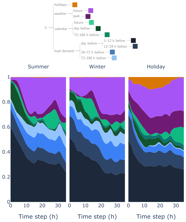
We emphasize that the fundamental premise of the method is precisely that this partition is not known a priori. Refer to Figure 2 in comparison with Figure 1.
Figure 2.
Explainability obtained from the direct calculation of the Shapley values for the same in Figure 1.
Remark 3.
Computational cost comparison: The computational complexity of KernelSHAP is exponential in n, where n is the number of features—in our case, interpretable components. For practical purposes, it is more convenient to consider the computational cost, which is given by , where represents the time required to evaluate a single prediction and is the sample size used for the masking values. To compute the exact Shapley values for an instance, the algorithm must solve a weighted linear regression over all possible feature coalitions. Because the exact method is computationally expensive, practical implementations rely on Sampled KernelSHAP. Instead of generating all combinations, this approach draws a fixed number of samples. Specifically, the standard SHAP library implementation sets this number of samples to for , and by default for , where n is the number of features. The computational cost of Sampled KernelSHAP is given by . On the other hand, to estimate the computational cost of our method and simplify the exposition, we can assume, without the loss of generality, that the branching factor remains constant across both the initial step and each subsequent close-up. If is the number of close-ups executed during the procedure, then the total number of coalitions is given by . Since the number of interpretable subcomponents estimated during the process is , the computational cost in terms of n is
For any n, the branching factor can be bounded to maintain a manageable computational cost while even ensuring an asymptotic linear behavior with respect to n. For small n, Sampled KernelSHAP essentially involves all the possible coalitions.
This latter scenario aligns naturally with our method. Indeed, as established in George A. Miller’s seminal 1956 article [13], the human information processing capacity is limited to seven items or categories, plus or minus two. This cognitive limit is managed through chunking, a technique that organizes independent units of information into meaningful blocks.
4. Case Study: Short-Term Load Forecasting
Our case study is based on a real production model for CENACE (National Energy Control Center, Mexico). The system receives calendar data (hour, day, and month), demand data from the Northwest Regional Control Zone in Mexico, temperature and apparent temperature variables from 10 load zones across different cities aggregated into a single variable, and finally, binary data corresponding to 10 holidays. Using this information, the system generates an hourly multivariate time series comprising 15 variables, scaled to the interval to be consistent with the model’s input requirements.
The implemented model f is a sequence-to-sequence model based on an LSTM encoder–decoder neural network. Both the encoder and decoder consist of a sequence of connected LSTM units. The encoder has 100 hidden states and an input sequence window of 180 h. The decoder also features 100 hidden units and a 36 h time window. The encoder’s task is to capture the underlying patterns of the input sequence, while the decoder processes the look-ahead data to generate the output sequence.
Specifically, the inputs are of the form ; the encoder accepts matrices of the form corresponding to 180 h with information from the “past” corresponding to the 15 variables, and the decoder receives calendar, weather, and holiday information in advance. The model output is a vector with the forecast of the energy demand for the next 36 h. The parameter vector was tuned on a training set of 118,969 data pair-points (1 January 2010 00:00 to 6 August 2023 23:00).
4.1. Experimental Comparison with KernelSHAP
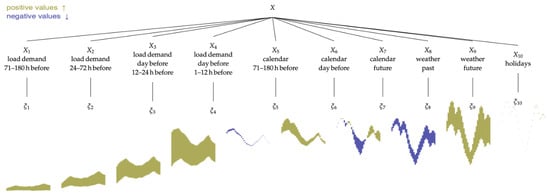
In an initial experiment, we evaluated the robustness of the method with respect to the sample size used for masking. We compared this stability against KernelSHAP and reported the execution times for both approaches. In this experiment, we utilized the explainability tree topology shown in Figure 1; consequently, the resulting explainability vectors consisted of 10 final interpretable components. Since the number of components was less than 11, KernelSHAP avoids random sampling and solves the weighted least squares problem using the exhaustive set of all possible coalitions.
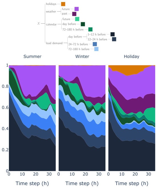
To this end, we considered three distinct relevance profiles within our context by randomly selecting three inputs X corresponding to summer, winter, and holiday. Specifically, tests were conducted using sample sizes of 100, 500, and 1000. Since these samples were selected at random, the experiment was repeated using five different random sample sets for each sample size. Figure 3 shows the three considered input profiles.
Figure 3.
Contributions of the 10 final interpretable components over the 36 h forecast horizon for the configuration across three distinct input profiles. The profile of holiday corresponds to the Christmas season.
Our empirical findings, reported in Table 2, reveal the following: (1) The standard deviation of the estimated explainability values across the five repetitions decreased as the sample size increased, though not significantly. In fact, even with a sample size of 100, the standard deviation was on the order of , which we considered acceptable within this context; indeed, this is practically the same stability achieved by the KernelSHAP method. (2) We observed that the processing times were significantly shorter when estimating the explainability tree. The experiments were executed on an Apple M4 computer with 16 GB of RAM. For instance, for 100 samples, the KernelSHAP method took approximately 112 s, whereas our proposed method took less than 4 s in all cases. This is consistent with the fact that the execution time depends on the sample size of and the number of model calls. Indeed, in all cases, the KernelSHAP algorithm called the model 2046 times, while our method only called it 70 times.
Table 2.
Robustness results with respect to sample size with execution time. Three different days from the test set were evaluated using 5 random sample sets per sample size.
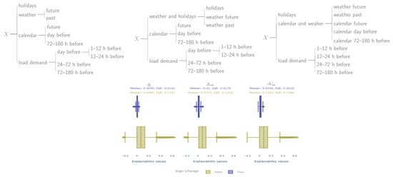
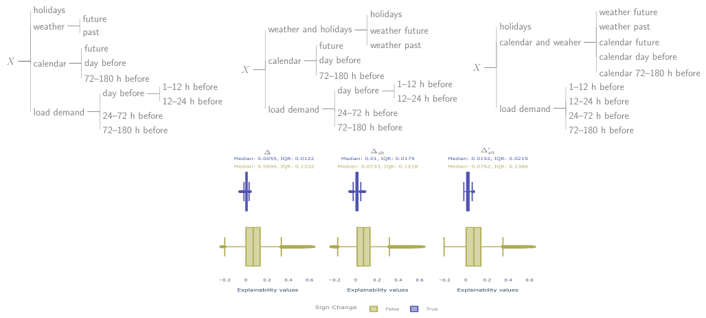
When addressing the question regarding the relationship between the explainability vectors provided by the tree and the output relative to the baseline Shapley values, the experiments demonstrated that the coherence of the explainability remained essentially invariant. Indeed, for this test, we used a sample of 100 elements from for the masking process. Additionally, we conducted the exercise with alternative topologies, and . See Figure 4. The results are shown in Table 3.
Figure 4.
Distribution of explainability values given by our method for configurations , , and , categorized by sign change with respect to the sample KernelSHAP method.
Table 3.
Coherence of KernelSHAP explainability with respect to the , , and configurations using the same 10 final interpretable components. The experiments were based on 50 randomly selected input vectors over a one-year period.
For the three tree configurations, the average difference between the explainability vectors obtained with Sample KernelSHAP was approximately . We also measured the percentage of sign changes in the explainability values between the proposed method and KernelSHAP. This percentage increased from 5.6% to 9.0%. However, as shown in Figure 4, the distribution of the explainability values that change sign revealed that they were around ten times smaller than those that maintained their sign. A substantial portion of these consisted of values very close to zero.
We computed the Spearman rank correlation coefficient between the Shapley vectors obtained via KernelSHAP and the explainability vectors from the proposed hierarchical method to quantify differences in the importance ranking of the interpretable components. Specifically, we analyzed the ordering of the explainability values for each of the 10 interpretable components across the 36 h forecasting horizon, resulting in a comprehensive ranking of these 360 values. Alignment with the KernelSHAP ordering was remarkably high, exceeding 0.96 across all three tree configurations.
The total variance of the contributions was computed over a sample of 50 inputs throughout the year for configuration . The results demonstrated that the variability was heavily dominated by future-horizon features, with weather-futureand calendar-future accounting for and , respectively. Short-term historical features exhibited moderate contributions, where calendar-day before represented and load demand 1–12 h before captured . Conversely, the remaining components—including holiday—collectively contributed just to the total variance. This does not imply that the methodology does not react to holidays, as illustrated in the third profile in Figure 3; rather, because there are very few holidays throughout the year, their overall variance contributions are generally negligible.
We repeated the exercise by omitting the error correction for configuration . Due to the relatively small magnitude of the error, the explainability narrative expectedly remained unchanged compared to the direct calculation via KernelSHAP. For instance, the Spearman coefficient shifted on average from to . Furthermore, the rate of sign changes was even lower without error correction, dropping from 5.6% to 4.6%, affecting—once again—values very close to zero. However, without error correction, the hierarchical structure was lost, and the average distance to the Shapley values increased slightly, moving from to .
Regarding the out-of-distribution samples for masking (Remark 1), we conducted tests by restricting the background sampling strategy to “similar inputs.” Specifically, we looked at days from the same season to minimize unrealistic feature combinations, such as combining future summer weather of 26–44 °C (78.8–111.2°F) with past winter weather of 8–24 °C (46.4–75.2°F). We generated five sets of 100 random samples using historical data from previous years, corresponding to the same month as the selected summer day. To explore the sampling effect, we calculated the standard deviation across the five selective random samplings relative to the mean value of the five general random samplings. In our case, the resulting standard deviation was . This value is comparable to the intrinsic variability among the random samples themselves, as shown in Table 2. Although we observed no significant differences in this case, it is possible that, under another scenario, it could be an element requiring special attention, especially if the explainability is linked to sensitive matters.
4.2. Granular Analysis via Multiple Close-Ups
We considered the initial decomposition rule:
To describe the interpretable components more easily, let us consider the timeline . We assume that discrete encoder events are contained within the segment (representing the 180 past hours), while decoder events are in the segment (representing the 36 future hours). The interpretable component involves only values within , whereas the remaining components span the interval . We compute , , , and to set the stage for the explanation of . The final explainability tree T is obtained by applying consecutive close-ups. We state that an iteration n is complete when the largest height-n subtree of T has been constructed.
For this analysis, the explainability vectors were calculated using a random sample of 100 data points from the training set. The average contribution of this component across all forecasted hours accounted for only 0.06% of the sum of the average contributions of all initial components. In contrast, , , and accounted for 72.75%, 22.69%, and 4.56%, respectively. Therefore, we omitted the further analysis of this interpretable component.
For the remaining initial components, we constructed subcomponents by partitioning the original time interval into disjoint subintervals. For each hour , we considered a function defined over the corresponding time interval , which is progressively refined at each iteration. This function is piecewise constant across the subintervals , such that the signed area under the curve within each subinterval equals . By the breakdown contribution property, it holds that, regardless of the iteration,
Consequently, each iteration provides a more detailed breakdown of the initial component’s contribution over time, allowing the resolution to be adjusted as needed and the focus to be placed exclusively on specific regions of interest.
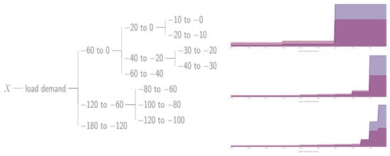
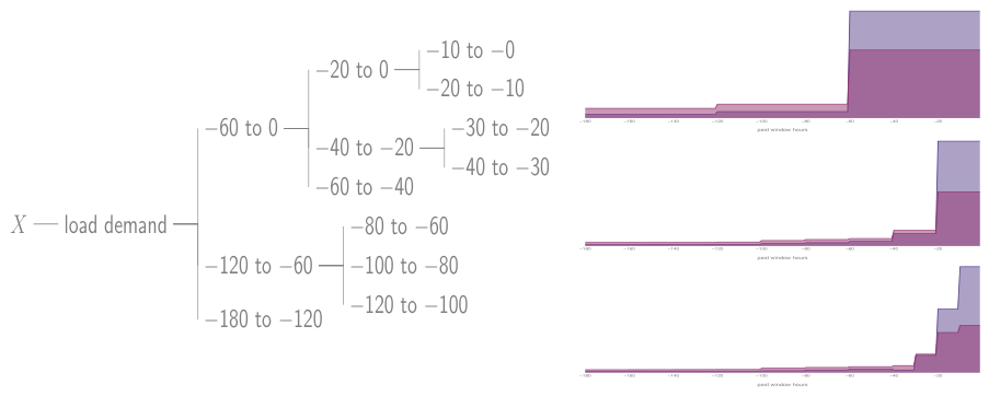
In Figure 5, we present the resulting functions and for a nine-subcomponent leaf subtree generated after three iterations. The close-ups exhibit a consistent and coherent profile across all time points, with a substantial shift occurring within 30 h prior to the forecast—the exact point at which the importance of historical events begins to diminish significantly. We observed that the longer the forecast horizon, the less importance was attributed to past events. Indeed, activities from the distant past remained negligible when examining these close-up visualizations.
Figure 5.
Explainability subtree for and its corresponding SHAPE functions for forecast hours 1 and 36 across tree iterations. On the right side are the results of the three iterations of the functions (purple) and (magenta).
With respect to , we considered an 18-subcomponent leaf subtree generated after three iterations, where 12 of these subcomponents correspond to decoder close-ups. We observed that the greatest contribution was distributed between 72 h prior to the forecast and the future calendar data known in advance. For these future calendar features, the first 18 h of the decoder concentrated the contribution—exhibiting negative values—precisely on those same forecast hours. Furthermore, the last 18 h of the decoder captured the small remaining contribution, affecting only the final hours of the forecast horizon.
For , we considered the same tree as . In the first iteration of the analysis for , we observed that the greatest contribution was distributed between 72 h prior to the forecast and the future calendar data known in advance. In the second iteration, we observed that the contribution from the past was actually focused within the last 24 h prior to the forecast. Interestingly, exploring the decoder calendar data revealed that the explainability value of corresponding to the component was nearly zero (); however, close-ups from the subsequent iteration indicated that this behavior does not imply that all subcomponents within that interval possess equally negligible values, but rather that their opposing contributions (on the order of ) mutually cancel out. For , no further close-up analysis was required. In this analysis, the results remained consistent across the various close-ups along the temporal horizon.
For this exercise, it was necessary to consider only 352 coalitions, rather than the that would have resulted from applying the sample KernelSHAP method to estimate the Shapley vectors, assuming that the configuration of was known in advance.
5. Conclusions
We present a model-agnostic framework for explaining the contributions of an input X to a forecast , building upon the principles of LIME and SHAP. The proposed methodology allows analysts to refine the explanations hierarchically to the extent required by the specific problem context, thereby generating a multi-resolution explainability narrative.
We evaluated the method on two alternative tree configurations that yielded the same final components. Furthermore, it should be noted that the initial full configuration was, in fact, an extreme scenario. We report that the coherence of the explainability was successfully maintained for these cases, as shown in Table 3. This outcome aligns with our intuitive expectations; although the explainability tree inherently depends on its topology throughout the process, numerous masked values remain coincident as long as the final interpretable components are identical. Naturally, the exact variance may change depending on the context and the complexity of the input. To assess the robustness and reliability of the method against analyst-dependent refinement in a real-world scenario, several configurations can be implemented. For instance, one can evaluate alternative tree configurations that yield the same final components in order to verify whether the methodology is reliable for that specific use case.
Finally, while this method does not preserve all axioms of Shapley values and inherits some of their weaknesses, we highlight its practical utility under certain conditions due to the following advantages:
- Computational efficiency control: The precise management of the execution time via the branching factor is enabled, even in scenarios requiring high-resolution or detailed explanations.
- Straightforward practical implementation: For every close-up, the workflow only requires a dictionary specifying the partitions of the input X and a concatenation function to reconstruct a valid input for f. Consequently, the identical core procedure can handle the initial and inductive steps for any partition dictionary or assembly function.
- Architecture-agnostic deployment: Since the framework does not depend on the internal structure of f, it can be seamlessly integrated into the production pipeline of a forecasting cycle. This setup requires minimal configuration changes for different models, utilizing a unified engine as a complement to continuous forecast monitoring.
- Flexible design-stage exploration: During the model development phase, it serves as a versatile tool for exploring the behavioral dynamics of f, providing actionable insights for model refinement and tuning.
- Automation and adaptability potential: The underlying methodology provides a foundation for developing automated pipelines for generating explainability trees, e.g., it is possible to consider trees with a fixed branching factor and a desired minimum level of granularity to obtain an “unsupervised” explainability map.
Author Contributions
Conceptualization, O.G. and J.W.; methodology, O.G.; software, O.G. and J.W.; formal analysis, O.G.; investigation, O.G.; data curation, J.W.; writing—original draft preparation, O.G.; writing—review and editing, O.G. and J.W.; project administration, J.W. All authors have read and agreed to the published version of the manuscript.
Funding
This research received no external funding.
Institutional Review Board Statement
Not applicable.
Informed Consent Statement
Not applicable.
Data Availability Statement
The data, code, and models used in this work are available in the GitHub repository https://github.com/mcd-unison/explaniability-forecasting-with-close-up (accessed on 13 October 2026).
Acknowledgments
We would like to thank the forecasting team at CENACE (National Energy Control Center, Mexico) in the northwest region, especially Héctor Gutiérrez Ibarra and Manuel Verdugo Vázquez, for the data they provided and their feedback on the presented explainability model.
Conflicts of Interest
The authors declare no conflicts of interest.
Abbreviations
The following abbreviations are used in this manuscript:
| LIME | Local Interpretable Model-Agnostic Explanation |
| LSTM | Long Short-Term Memory |
| SHAP | Shapley Additive Explanation |
| STLF | Short-Time Load Forecasting |
Appendix A. Proofs
Let f be a trained model and X be an input to f. Let , and for every , let be the vector in given by the inductive rule.
- 1.
- Breakdown contributions:
- 2.
- For every , the values are the Shapley values for the game where is given by the Formula (1). Indeed, let be considered at any iteration of the inductive process such that (where may not exist). The general form of the weighted least squares solution is given by:where C is the matrix of binary coalitions, W is the diagonal matrix with weights for each row in X, and matrix Y is a with a row for each . Note that, for each z, , whereTherefore, the columns of Y given by are vectors of values. For each we can follow point by point the proof of Theorem 2 in [2] [Supplemental Material]; from each —since the arguments are independent of the specific definition of —we can conclude that entries in the t-th column of , namely , are the Shapley values for the game with
- 3.
- Local symmetry. The local marginal contribution of an interpretable subcomponent for a coalition such that is defined as:where is the coalition resulting from changing to . Suppose for . For every , by the Shapley value properties of the game , we have , which implies that , and thus, .
- 4.
- Global efficiency. By the breakdown contribution property, we can calculate in a bottom-up manner through the tree. Furthermore, the tree can be simplified at each step:
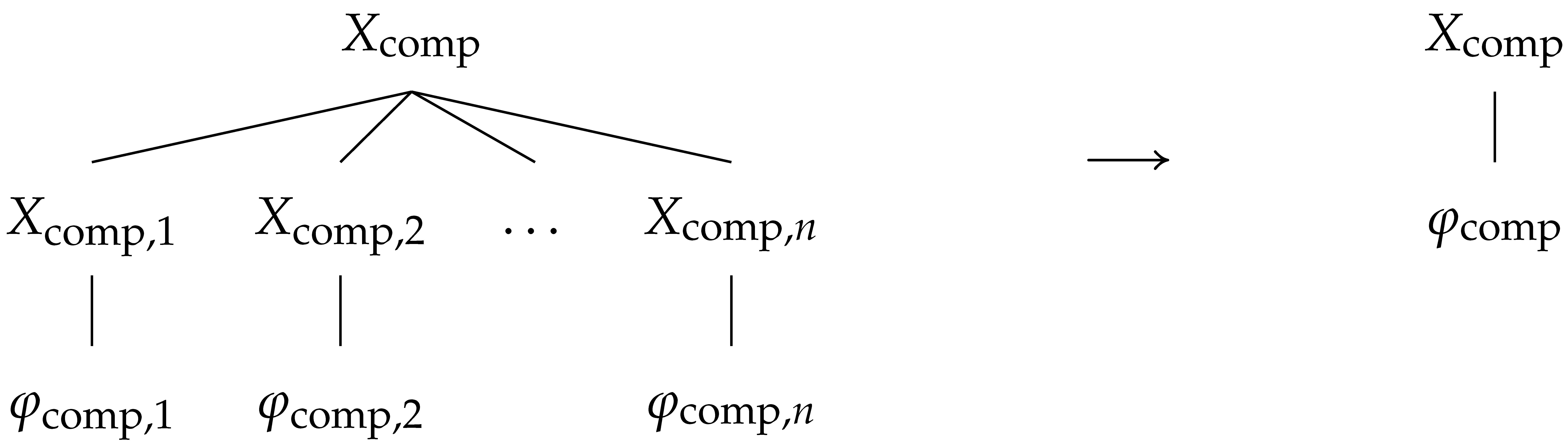 In the last step, we get the vector sum , which is indeed .
- 5.
- Global nullity with error. The global marginal contribution of an interpretable subcomponent for a coalition such that is defined as:where is the global index of . Suppose that . Note that, for , we can define such that the indices of coincide with those of u for the sub-components in , and are set to 1 otherwise. Let u be such that its i-th index is 0. For each , and . Then, , and by the properties of Shapley values, , for each . Therefore, and so .
References
- Štrumbelj, E.; Kononenko, I. A general method for visualizing and explaining black-box regression models. In Proceedings of the 10th International Conference on Adaptive and Natural Computing Algorithms—Volume Part II; ICANNGA’11; Springer: Berlin/Heidelberg, Germany, 2011; pp. 21–30. [Google Scholar]
- Lundberg, S.M.; Lee, S.I. A unified approach to interpreting model predictions. In Proceedings of the 31st International Conference on Neural Information Processing Systems; NIPS’17; Curran Associates Inc.: Red Hook, NY, USA, 2017; pp. 4768–4777. [Google Scholar]
- Ribeiro, M.T.; Singh, S.; Guestrin, C. “Why Should I Trust You?”: Explaining the Predictions of Any Classifier. In Proceedings of the 22nd ACM SIGKDD International Conference on Knowledge Discovery and Data Mining; KDD ’16; Association for Computing Machinery: New York, NY, USA, 2016; pp. 1135–1144. [Google Scholar] [CrossRef] [Scilit]
- Bento, J.; Saleiro, P.; Cruz, A.F.; Antunes, L.M.; Bizarro, P. TimeSHAP: Explaining Recurrent Models through Sequence Perturbations. In Proceedings of the 27th ACM SIGKDD Conference on Knowledge Discovery & Data Mining; ACM: New York, NY, USA, 2021; pp. 2565–2573. [Google Scholar] [CrossRef] [Scilit]
- Nayebi, A.; Tipirneni, S.; Foreman, B.; Reddy, C.K.; Subbian, V. WindowSHAP: An efficient framework for explaining time-series classifiers based on Shapley values. J. Biomed. Inform. 2023, 144, 104438. [Google Scholar] [CrossRef] [Scilit] [PubMed]
- Jiang, Y.; Zhang, Y.; Shen, Y.; Zhao, Y.; Sun, C.; Wu, J.; Wen, L. SeqSHAP: Subsequence Level Shapley Value Explanations for Sequential Predictions. In Proceedings of the DASFAA; Springer: Berlin/Heidelberg, Germany, 2024; pp. 249–266. [Google Scholar] [CrossRef] [Scilit]
- Tucker, A.; Swift, S.; Liu, X. Variable grouping in multivariate time series via correlation. IEEE Trans. Syst. Man, Cybern. Part B (Cybern.) 2001, 31, 235–245. [Google Scholar] [CrossRef] [Scilit] [PubMed]
- Keogh, E.; Chu, S.; Hart, D.; Pazzani, M. Segmenting time series: A survey and novel approach. In Data Mining in Time Series Databases; World Scientific: Singapore, 2004; pp. 1–21. [Google Scholar] [CrossRef] [Scilit]
- Cover, T.M.; Thomas, J.A. Elements of Information Theory, 2nd ed.; Wiley-Interscience: Hoboken, NJ, USA, 2006. [Google Scholar]
- Shapley, L.S. A Value for n-Person Games. In Contributions to the Theory of Games, Volume II; Kuhn, H.W., Tucker, A.W., Eds.; Princeton University Press: Princeton, NJ, USA, 1953; Volume 28, pp. 307–317. [Google Scholar]
- Kumar, I.E.; Venkatasubramanian, S.; Scheidegger, C.; Friedler, S.A. Problems with Shapley-value-based explanations as feature importance measures. In Proceedings of the 37th International Conference on Machine Learning; ICML’20; JMLR.org: Norfolk, MA, USA, 2020. [Google Scholar]
- Slack, D.; Hilgard, S.; Jia, E.; Singh, S.; Lakkaraju, H. Fooling LIME and SHAP: Adversarial Attacks on Post hoc Explanation Methods. In Proceedings of the AIES 20: Proceedings of the AAAI/ACM Conference on AI, Ethics, and Society; Association for Computing Machinery: New York, NY, USA, 2020; pp. 180–186. [Google Scholar] [CrossRef] [Scilit]
- Miller, G.A. The magical number seven, plus or minus two: Some limits on our capacity for processing information. Psychol. Rev. 1956, 63, 81–97. [Google Scholar] [CrossRef] [Scilit]

Disclaimer/Publisher’s Note: The statements, opinions and data contained in all publications are solely those of the individual author(s) and contributor(s) and not of MDPI and/or the editor(s). MDPI and/or the editor(s) disclaim responsibility for any injury to people or property resulting from any ideas, methods, instructions or products referred to in the content. |
© 2026 by the authors. Licensee MDPI, Basel, Switzerland. This article is an open access article distributed under the terms and conditions of the Creative Commons Attribution (CC BY) license.