


Abstract
Residue-soil mixing and reduced spectral sensitivity complicate summer maize leaf area index (LAI) estimation from unmanned aerial vehicle multispectral imagery. We compared full-plot and canopy domains, paired differences, neighborhood statistics, and approximate days after sowing (DAS), calculated from a common reference date. Five input schemes (B0–B4) and four algorithms were evaluated using 345 samples collected on five dates in one growing season. Spatial validation comprised ten repetitions of five-fold grouped cross-validation, with preprocessing and feature selection restricted to training data. For gradient boosting decision trees, R2 increased from 0.515 for B0 to 0.686 for B3 and 0.846 for B4, whereas RMSE decreased from 0.834 to 0.671 and 0.470. Low-LAI Bias decreased from 0.580 to 0.343 and 0.160. Fixed-capacity controls supported conditional improvements after adding paired differences and neighborhood statistics. Approximate DAS produced the largest sequential RMSE reduction, mainly through between-date adjustment. Time-baseline and training-fold residual analyses distinguish calendar-time adjustment from within-date predictive information. High-LAI underestimation and unseen-date errors delimit application beyond the sampled dates and production-field conditions. Within this defined scope, the framework provides a reproducible comparison of image-domain representations under heterogeneous production conditions.
1. Introduction
Leaf area index (LAI), defined as the one-sided leaf area per unit ground area, is an important biophysical parameter linking canopy radiation interception, evapotranspiration, photosynthesis, and crop growth status. It is also a key remote-sensing variable for crop growth monitoring and field management [1]. Ground instruments and destructive measurements can provide plot-scale reference values, but their measurement efficiency, observation geometry, and spatial representativeness limit continuous application at the field scale [2]. Satellite remote sensing provides regional coverage, yet it is often constrained by revisit intervals, cloud contamination, and mixed pixels. Precision agriculture therefore requires data sources that balance temporal scheduling, spatial resolution, and observation cost [3], and the value of field remote sensing depends on whether the information can be linked to actual management units [4]. UAVs can acquire centimeter-level, multi-temporal reflectance imagery during key growth stages, supporting LAI estimation at a scale closer to ground sampling. However, radiometric correction, geometric consistency, and observation conditions must still be strictly controlled [5,6]. This study examines how the statistical domain of UAV imagery affects LAI error at different canopy stages.
Existing remote-sensing approaches for crop LAI estimation can be broadly grouped into physical models, empirical vegetation indices, and sample-driven models. Physical models connect leaf optical properties, canopy structure, and reflectance through canopy radiative transfer processes. They have clear mechanistic interpretability, but the inversion results can be affected by prior parameters, equifinality, and observation geometry [7,8]. Empirical vegetation indices are easy to calculate and map, and combinations of multispectral red-edge and near-infrared bands have been used for maize LAI estimation [9]. The PROSAIL model, which couples the leaf optical properties model PROSPECT with the canopy radiative transfer model SAIL, can also be combined with UAV multispectral imagery to expand the spectral response range when training samples are limited [10]. Sample-driven methods use nonlinear regression to integrate spectral bands, vegetation indices, and spatial statistical information. Previous maize studies have shown that combining spectral and image spatial statistics can improve LAI estimation [11], but model performance still changes markedly across growth stages and complex smallholder-field backgrounds [12]. Multi-source data fusion and hyperspectral–multispectral comparisons further indicate that new information is useful only when the added features provide new canopy information, rather than simply increasing input dimensionality [13,14]. These studies provide several viable routes, but they have not directly clarified the respective roles of full-plot statistics, canopy statistics, and their inter-domain differences. GBDT sequentially fits regression trees to reduce prediction error [15], whereas RF averages randomized trees [16]. SVR uses a kernel-based regression function [17], and Ridge regularizes linear coefficients [18]. Recent maize studies examine multisource UAV features [19], hyperspectral and accumulated-temperature information across sowing dates [20], and computer-vision representations [21]. These examples motivate comparing model classes and input representations without assuming equivalent transferability.
The unresolved issue is most evident when sparse early canopies coexist with a residue background. Existing studies usually either calculate statistics from all pixels within a fixed plot or remove background first and retain only canopy pixels. The first strategy allows residue and bare-soil reflectance to enter the model. Simulation and ground observations have shown that residue cover can substantially alter canopy reflectance and vegetation indices in the low-LAI range [22]. The second strategy reduces the influence of pure soil pixels, but it may also remove information related to vegetation cover and inter-row structure. In UAV maize imagery, the proportion of soil background has been identified as an important source of early-stage LAI uncertainty [23]. Under rice-wheat rotation residue backgrounds, a specially designed residue-soil-adjusted red-edge index mainly improved low-LAI estimation [24]. The difficulty is that soil type, canopy structure, and background spectra jointly alter the LAI-reflectance relationship [25], while residue and soil cannot always be stably separated in the visible to near-infrared range [26]. Recent multi-platform experiments also show that soil moisture, residue, shadow, and canopy cover jointly affect vegetation indices [27]. Without placing the full-plot domain, canopy domain, and inter-domain differences into the same progressive control framework, it is difficult to determine whether low-LAI overestimation originates from model form, input dimensionality, or a mismatch between the image statistical domain and the green canopy. As a result, the overall accuracy may appear acceptable, while LAI can be systematically overestimated during early management stages.
This study compares full-plot and canopy-domain representations to examine how background screening, paired differences, and neighborhood information affect LAI estimation. Calendar-time information is evaluated separately to distinguish between-date adjustment from within-date prediction. Spatially grouped validation addresses prediction at new locations on dates represented in training [28]. Unseen-date prediction is assessed as a separate sensitivity analysis.
We address three questions: how inter-domain spectral contrasts vary across observation dates; how prediction changes across spectral representations under matched comparisons; and how approximate DAS affects overall and within-date performance. We also examine low- and high-LAI errors and distinguish spatial prediction on represented dates from prediction on unseen dates. Overall, R2 describes predictive performance across the pooled observations, while RMSE, Bias, and Slope characterize errors within restricted LAI ranges.
2. Materials and Methods
2.1. Study Area and Observation Design
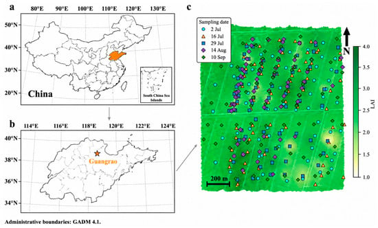
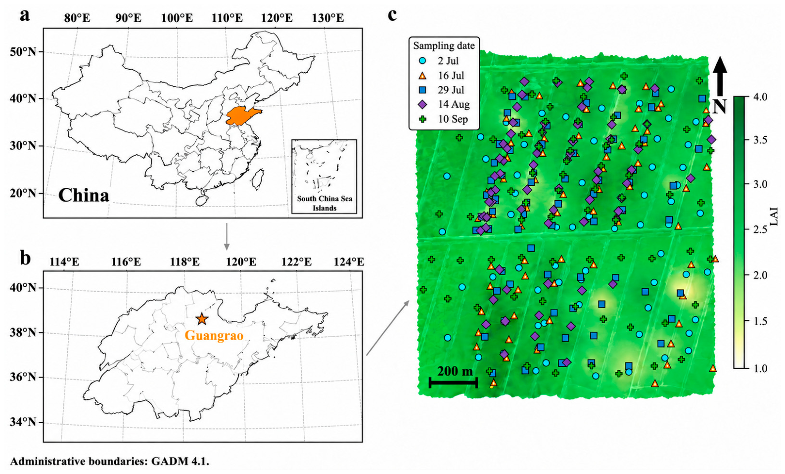
The study was conducted in Guangrao County, Dongying City, Shandong Province, China (sample center approximately 37°12′58″ N, 118°32′10″ E). The area lies on the Yellow River Delta alluvial plain and has a warm-temperate monsoon climate. Samples were collected from farmer-managed summer maize fields under winter wheat-summer maize rotation, with wheat residue retained at the soil surface. The fields were independently managed by multiple farmers rather than subjected to one prescribed experimental treatment. Cultivar or hybrid, planting density, row spacing, fertilization, irrigation, crop protection, and actual sowing date consequently varied among fields; complete field-level records were not available for consistent reporting. This production-field setting enabled the method to be evaluated across management conditions encountered in local farming practice. For consistency with the original analysis, DAS denotes an approximate calendar-time reference calculated from 1 June 2025, rather than verified field-specific days after sowing. Figure 1c displays all five sampling dates over an LAI surface interpolated only from the 29 July observations; this background is retained solely as spatial context and does not represent the other dates.
Figure 1.
Location of the study area and sampling points. (a) Shandong Province within China; (b) Dongying City, Guangrao County, and the sampled production fields; (c) sampling locations from all five dates over an LAI surface interpolated from the 69 observations on 29 July 2025. Point colors identify sampling date. The background surface is single-date spatial context and is not interpreted as LAI on the other four dates.
Five UAV campaigns and corresponding ground LAI observations were conducted on 2 July, 16 July, 29 July, 14 August, and 10 September 2025. Of 347 records, two from the second campaign were excluded under an objective coordinate-validity check because their recorded longitudes fell outside the valid geographic range of −180° to 180°; one was a malformed coordinate with a missing decimal separator. The analysis retained 345 samples. Sampling locations were generally selected anew in each campaign, spanning a range of visually distinct canopy conditions across farmer-managed fields; they were not monitored as permanent plots. Table 1 summarizes the observations by date.
Table 1.
Sample size and LAI descriptive statistics for each observation date.
2.2. UAV Multispectral Imagery and Ground LAI
Five multispectral campaigns were conducted with a DJI Matrice 350 RTK platform (SZ DJI Technology Co., Ltd., Shenzhen, China) carrying a MicaSense RedEdge-P dual-camera multispectral system (AgEagle Aerial Systems Inc., Wichita, KS, USA). The system acquired ten bands. Of these, the five bands retained as analysis-ready orthomosaics in the original processing workflow were used consistently across all campaigns: blue (475 nm; 32 nm bandwidth), green (560 nm; 27 nm), red (668 nm; 14 nm), red-edge (717 nm; 12 nm), and near-infrared (842 nm; 57 nm). Flights were performed at 120 m above ground level and 8 m s−1, with 75% forward and side overlap and a nadir-looking camera. Image acquisition was scheduled between 10:00 and 14:00 under sunny, adequately illuminated, cloud-free and haze-free conditions, with wind speed below 10 m s−1. Raw images were processed in Pix4Dmapper (version 4.5.6; Pix4D SA, Prilly, Switzerland) for radiometric correction, aerial triangulation, and orthomosaic generation. Radiometric correction combined factory calibration parameters with ground reflectance calibration-panel data. The verified ground sampling distance ranged from 0.0765 to 0.0782 m, and all 25 band rasters used WGS84/UTM zone 50N (EPSG:32650). A 1 m × 1 m window was extracted around each sample coordinate.
Ground LAI was measured on each flight date using an LAI-2200C Plant Canopy Analyzer (LI-COR Biosciences, Lincoln, NE, USA), with field measurements synchronized as closely as practicable with the UAV campaign. At each sample point, one unobstructed above-canopy reference reading (A) was followed by six below-canopy readings (B) taken diagonally between maize rows, with the sensor held at the standard field position approximately 1 m above the ground and below the canopy. A 270° view cap was oriented away from the operator and direct sunlight. The six B readings were averaged and paired with the corresponding A reference in FV2200 software (version 2.1.1; LI-COR Biosciences, Lincoln, NE, USA) to calculate one LAI estimate for that point; they were not six independently calculated LAI estimates. Scattering correction was applied using the white scattering-correction accessory and the FV2200 procedure. No additional clumping or row-structure correction was applied. The LAI value reported by FV2200 was used as the reference variable for model development and evaluation.
2.3. Dual-Domain Representation, Paired Differences, and Multi-Scale Neighborhood Statistics
The full-plot domain comprised valid pixels in a 1 m × 1 m window centered on each sample. It included canopy, residue, soil, shadow, and mixed pixels. Canopy pixels were selected by NDVI-based Otsu thresholding [29]. Thresholds were estimated separately for observation dates represented in the current outer training fold. A pooled-training threshold served as the fallback when the target date was absent from training, as in LODO. Thresholds were fixed before predicting the corresponding validation samples. If no pixel passed the threshold, canopy statistics reverted to full-plot statistics and the event was recorded. Supplementary Table S1 reports these events separately for repeated spatial validation and LODO.
For each domain, band reflectance was averaged over the retained pixels. Vegetation indices were then computed from these domain-mean band values; they were not averages of pixel-wise index values. Corresponding full-plot and canopy statistics were denoted by Ffull and Fcanopy. Their paired difference was defined as
ΔF = Fcanopy − Ffull
ΔF represents the difference between two statistical descriptions of the same sampling window; the physical plot is unchanged. Neighborhood labels of 1 m and 2 m denote square-window side lengths centered on the sample coordinate. Band and NDVI means, standard deviations, ranges, and coefficients of variation summarize local variation. The 1 m neighborhood shares the support of the full-plot window. Consequently, highly correlated mean features were removed during within-family pruning at |ρ| ≥ 0.90, whereas the retained dispersion statistics provided distinct summaries of local reflectance heterogeneity.
2.4. Vegetation Indices and B0–B4 Feature Schemes
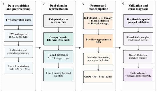
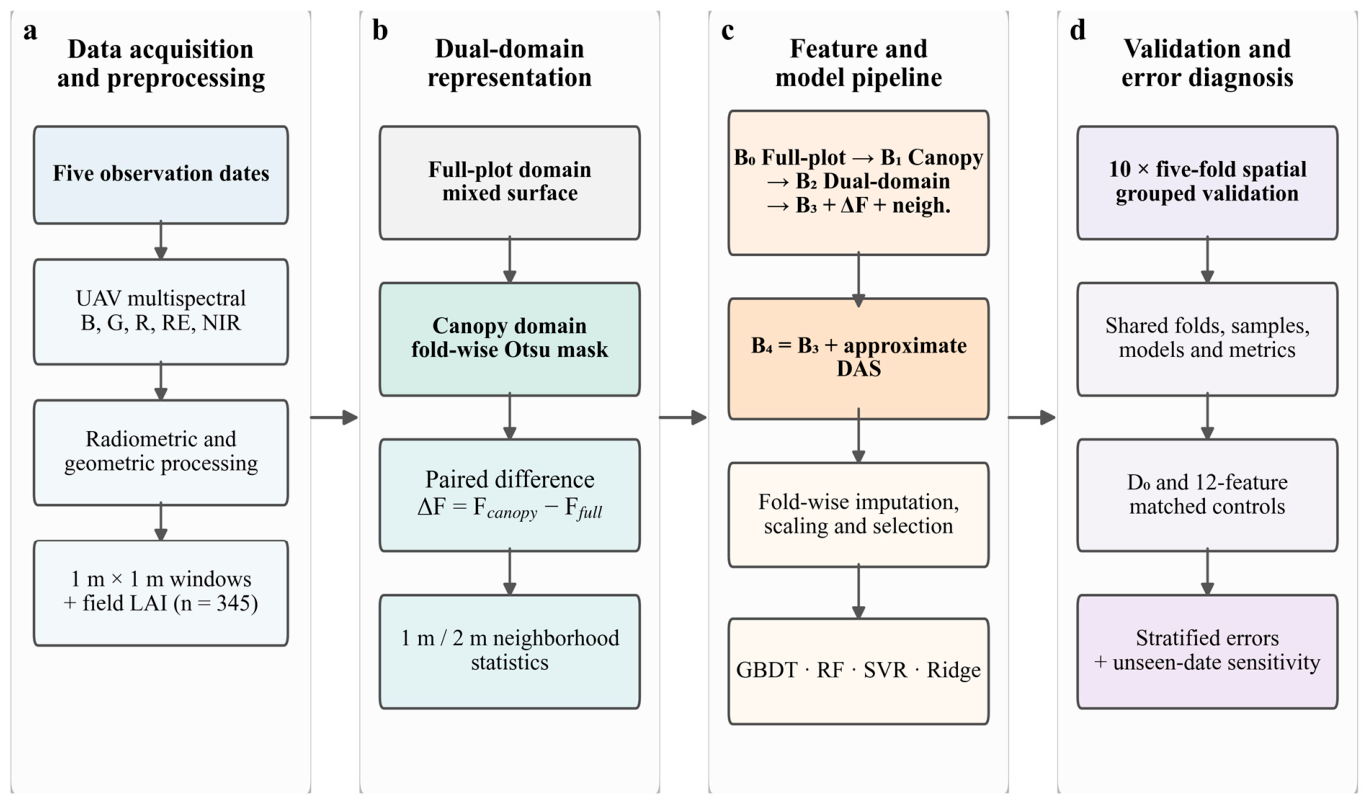
Candidate spectral features included five original reflectance bands and 20 vegetation indices, covering greenness, red-edge response, soil-background adjustment, chlorophyll sensitivity, and wide dynamic range. The applicable ranges and saturation issues of classical vegetation indices for LAI have been systematically discussed [30]. Based on the progressive relationship between the image statistical domain and additional information, five main schemes, B0–B4, were designed (Table 2). B4 introduced DAS only on the basis of B3, and the relationship among the schemes is shown in Figure 2c. The formulas and references for the 20 candidate vegetation indices are listed in Table 3.
Table 2.
Inputs and within-fold maximum number of selected features for the progressive B0–B4 schemes.
Figure 2.
Analysis workflow: (a) data acquisition and preprocessing; (b) dual-domain representation; (c) feature and model pipeline; and (d) validation and error diagnosis. Training-derived canopy thresholds, preprocessing, feature selection, and model fitting are confined to training data. The main spatial validation, fixed-capacity controls, sequential RMSE summaries, stratified errors, and unseen-date sensitivity analysis answer separate questions. Approximate DAS supplies calendar-time conditioning; the workflow does not impose a physiological growth curve or a physical constraint.
Table 3.
Vegetation indices used for LAI estimation, their formulas, and references.
2.5. Within-Fold Feature Screening and Model Pool
Feature screening was performed within each outer training fold. Missing values were replaced by training medians, with zero used for entirely missing columns. Constant features were removed. Relevance combined the absolute Spearman correlation with the univariate linear-regression F statistic from f_regression. Non-finite F values were set to zero, and positive F values were normalized by the maximum candidate F value. The composite score was S = 0.60|ρ| + 0.40Fnorm. The larger weight on |ρ| made the monotonic association with LAI the primary ranking criterion, while Fnorm supplemented it with univariate linear separation. The 0.60/0.40 ratio was used as a balanced engineering setting for these complementary criteria. Features were ranked by this score, and greedy pruning removed candidates with an absolute Spearman correlation of ≥0.90 with a retained feature within the same family. Inner spatial groups were formed from outer-training coordinates using K-means, with min(12, max(4, floor(ntrain/12))) groups and up to five GroupKFold splits. Selection frequency across inner training subsets defined stability. A frequency of 0.60 was the primary eligibility threshold. If a predefined feature family had no eligible member, its highest-ranked candidate could enter at a frequency of at least 0.40, preserving representation of that family against variation among inner spatial splits. The full algorithm, family quotas, seeds, and fallback rules are provided in Supplementary Methods S1. Standardization was fitted after selection. Outer-validation LAI values were not used for these operations.
The model pool included gradient boosting decision tree (GBDT) [15], random forest (RF) [16], support vector regression (SVR) [17], and ridge regression (Ridge) [18]. GBDT used 120 weak learners, a learning rate of 0.03, a tree depth of 2, a minimum of 8 samples per leaf node, and a subsampling ratio of 0.80. RF used 300 trees, a maximum depth of 6, a minimum of 6 samples per leaf node, and square-root feature sampling. SVR used a radial basis function (RBF) kernel with C = 10, ε = 0.10, and γ = scale. The α value of Ridge was set to 10. The same parameters were used for all feature schemes in the four model types, so that cross-scheme comparisons focused on differences in input information rather than on re-tuning.
2.6. Ablation Controls, Spatial Validation, and Leave-One-Date-Out Test
A difference-only control (D0) tested whether paired differences could replace absolute domain information. Separate fixed-capacity controls limited B2, B2+ΔF, B3, and B4 to at most 12 selected features, denoted B2(12), B2+ΔF(12), B3(12), and B4(12). D0 is a separate diagnostic, not the first step of a nested chain. The fixed-capacity comparisons shared spatial folds and GBDT settings. Their differences describe conditional changes under the stated selection procedure, rather than order-independent feature contributions.
To make the stepwise comparison in the main B0–B4 sequence explicit, we calculated the sequential relative RMSE reduction between adjacent schemes as
where k indexes the next scheme in the B0–B4 sequence. We also report the share of the total B0–B4 RMSE reduction as
Both quantities are descriptive and order-dependent. They are not independent feature contributions because the main schemes differ in input composition and maximum feature limits. The fixed-capacity controls were retained to assess module additions under a common upper limit.
Spatial groups were generated by K-means using projected sample coordinates in WGS84/UTM zone 50N (EPSG:32650), in meters. Each repetition used 25 groups, n_init = 10, and random_state = 1000 + r, where r ranged from 0 to 9. Twenty-five groups balanced spatial granularity with sufficient membership for five-fold validation: group sizes ranged from 3 to 28 samples, with a median of approximately 14 samples and a median group diameter of approximately 210 m. All groups therefore retained at least three samples, and ten repeated groupings reduced sensitivity to any single small-group allocation. GroupKFold assigned entire groups to five validation folds, and all models shared these assignments. The minimum and median validation-to-nearest-training distances were 11.2 and 89.2 m. Because K-means grouping does not impose an explicit separation buffer, we also evaluated 25 m and 50 m buffers. The corresponding B4 RMSEs were 0.469724 and 0.470910, compared with 0.469648 without an added buffer, showing that performance was nearly unchanged under these stricter distance settings. Main validation estimates prediction at new locations on dates represented in training [42].
LODO held out each observation date in turn and fitted preprocessing, canopy thresholds, feature selection, and models using the other four dates. It was not used for model selection. We describe it as unseen-date sensitivity analysis: holding out an intermediate date is temporal interpolation with respect to DAS, whereas holding out the earliest or latest date is extrapolation. Neither case is equivalent to the main spatial validation. Target samples may also differ in spectral conditions and LAI distribution [43]. A secondary threshold-transfer comparison replaced the pooled-training threshold with the nearest training-date threshold to assess the canopy fallback mechanism.
2.7. Evaluation Metrics and Error Stratification
For each repeat, all out-of-fold predictions were summarized to calculate the coefficient of determination (R2), root mean square error (RMSE), mean absolute error (MAE), Bias, and the predicted-versus-measured regression Slope:
Here, the observed and predicted LAI values are indexed by i; overbars denote their sample means, and n is the sample size. Positive Bias indicates overestimation. LAI and its absolute-error metrics are reported without area-ratio unit labels. Overall R2 measures predictive performance. Low-LAI (<1, n = 80) and high-LAI (≥3, n = 89) evaluation emphasizes RMSE, Bias, and Slope because restricted reference ranges can produce strongly negative stratified R2. Relative RMSE and Bias equal 100 times the corresponding absolute metric divided by the mean observed LAI in that subset (Supplementary Table S2). Metrics are summarized across ten complete repetitions, and error bars show descriptive between-repetition SD. Conditional spatial-block intervals for paired scheme differences and high-LAI slopes are reported in Supplementary Tables S3 and S4.
3. Results
3.1. Dual-Domain Differences Across Observation Periods
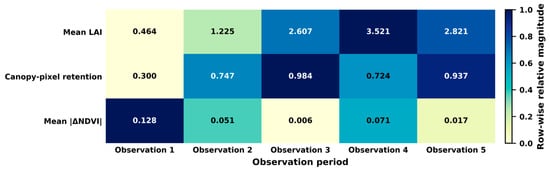
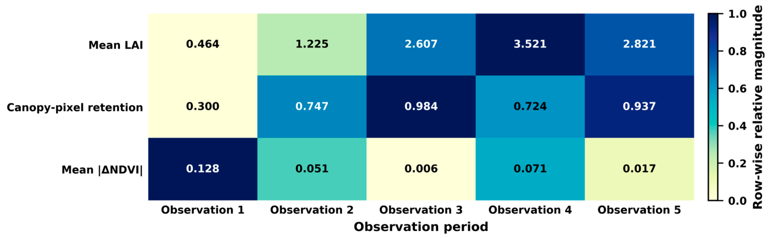
Mean LAI increased from 0.464 ± 0.129 in the first observation period to 3.521 ± 0.607 in the fourth observation period, and then decreased to 2.821 ± 0.477 in the fifth observation period during senescence. Low-LAI samples were mainly concentrated in the first and second observation periods. Early background mixing was therefore the main stage for testing low-LAI overestimation.
Dual-domain differences showed a clear stage pattern (Figure 3). In the first observation period, the mean proportion of retained canopy pixels was only 0.300, and mean |ΔNDVI| was 0.128. In the second observation period, these values changed to 0.747 and 0.051, respectively. In the third observation period, the retained canopy-pixel proportion increased to 0.984, and mean |ΔNDVI| decreased to 0.006, indicating that the full-plot domain and the canopy domain were close to each other. In the fourth observation period, the retained proportion decreased to 0.724 and mean |ΔNDVI| increased again to 0.071. In the fifth observation period, the two metrics converged again. These changes indicate that inter-domain differences were mainly concentrated in the early low-LAI stage and weakened markedly as canopy cover increased.
Figure 3.
Descriptive changes across five observation dates in mean LAI, retained canopy-pixel proportion, and mean absolute inter-domain NDVI difference. Values are printed in each cell. Colors are normalized within each row and therefore compare dates within a metric, not magnitudes among different metrics. These descriptive sample summaries are separate from the training-fold thresholds used for validation.
3.2. Overall Accuracy and Cross-Model Consistency
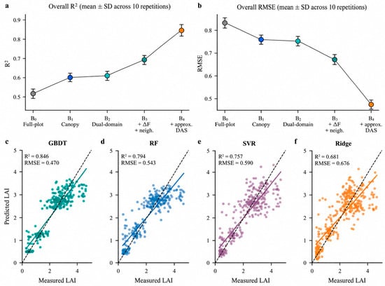
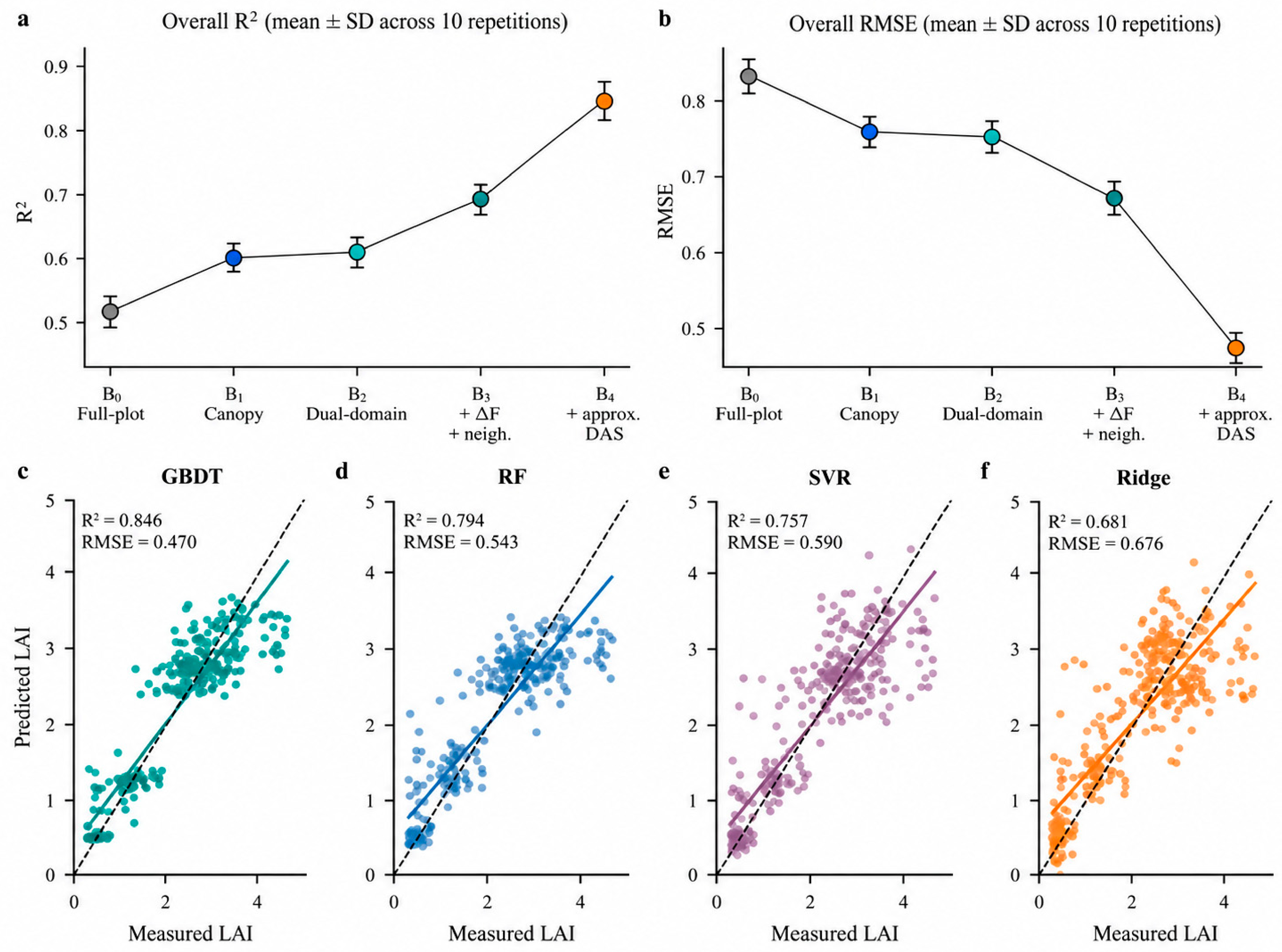
For GBDT, overall R2 increased from 0.515 for B0 to 0.598 for B1 and 0.605 for B2, further increased to 0.686 for B3, and reached 0.846 for B4 (Figure 4a; Table 4). The corresponding RMSE decreased from 0.834 to 0.759, 0.752, 0.671, and 0.470 (Figure 4b). Compared with B0, RMSE decreased by 19.6% for B3 and by 43.7% for B4.
Figure 4.
Main spatial validation. (a,b) GBDT R2 and RMSE, shown as means ± descriptive SD across ten repetitions. (c–f) Mean OOF predictions across repetitions for each of 345 samples under B4 with GBDT, RF, SVR, and Ridge. Colors identify the observation dates as in Figure 1; dashed lines show 1:1 agreement. Scatterplots show per-sample averages, whereas panels (a,b) summarize complete repetitions. Conditional paired intervals are reported in Supplementary Table S3.
Table 4.
Overall and stratified accuracy of GBDT under ten repetitions of five-fold spatial group cross-validation.
The cross-model results did not change the main conclusion. The R2 increments from B2 to B3 were 0.081, 0.080, 0.034, and 0.164 for GBDT, RF, SVR, and Ridge, respectively, and RMSE decreased by 0.081, 0.082, 0.035, and 0.145. The R2 increments from B3 to B4 were 0.160, 0.101, 0.070, and 0.063, respectively, and RMSE decreased by 0.201, 0.120, 0.080, and 0.064.
3.3. Early Low-LAI Overestimation and the Auxiliary Role of DAS
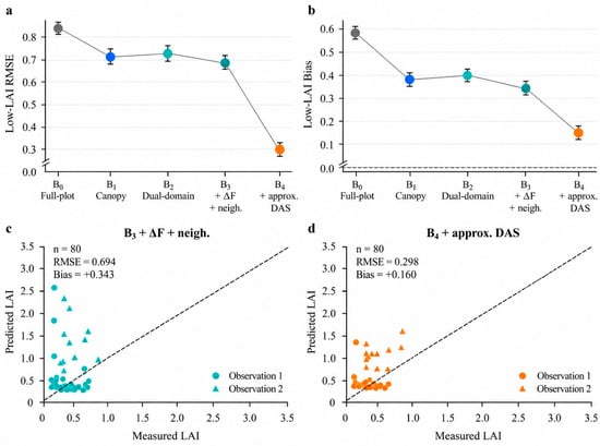
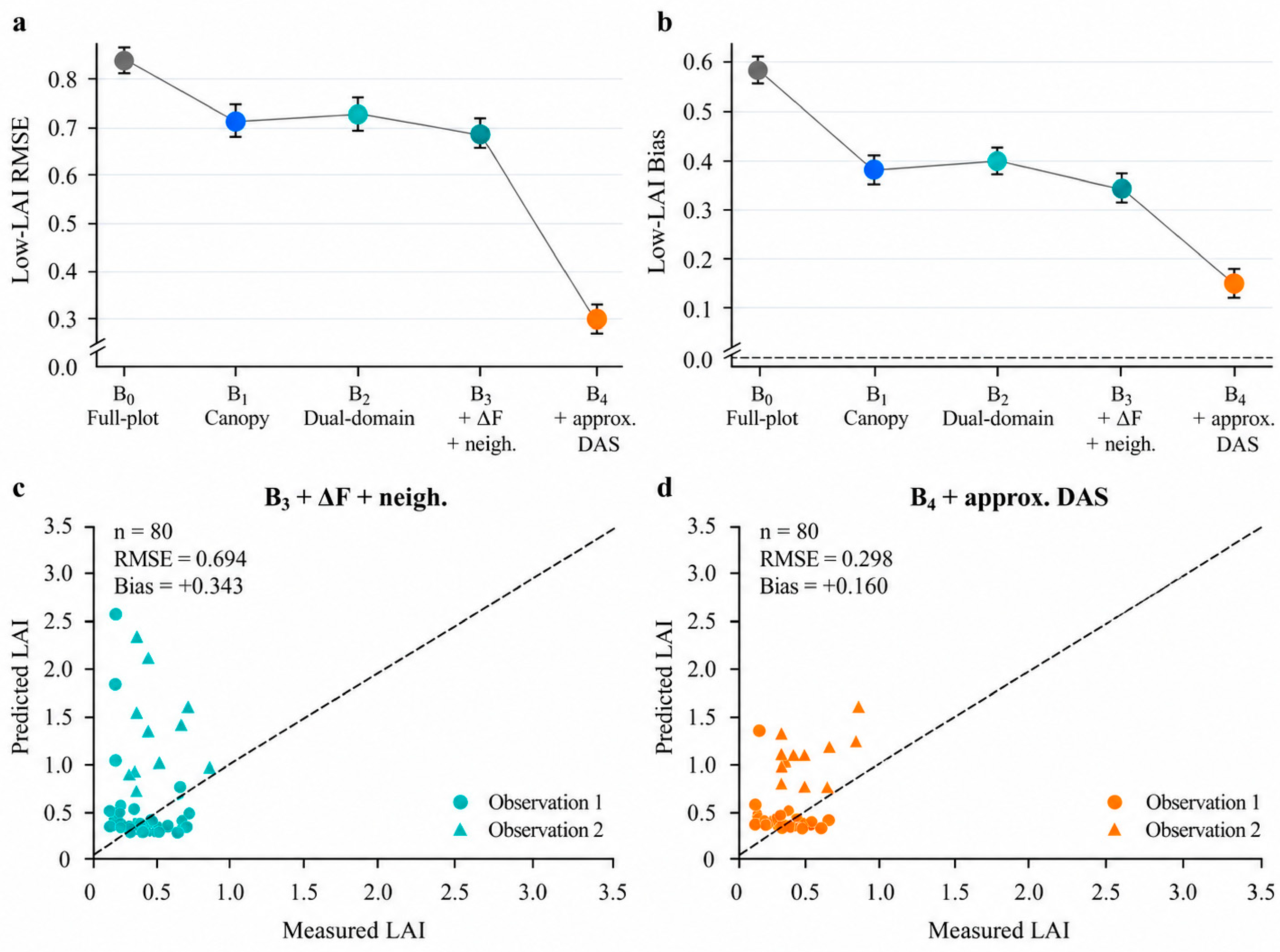
The low-LAI subset showed systematic overestimation. The RMSE and Bias of B0 were 0.843 and 0.580, respectively. B1 reduced them to 0.721 and 0.383, consistent with an initial benefit from canopy-domain screening. The RMSE/Bias values of B2 were 0.729/0.395, those of B3 decreased to 0.694/0.343, and those of B4 further decreased to 0.298/0.160 (Figure 5a,b). Compared with B0, B4 reduced low-LAI Bias by 72.4%.
Figure 5.
Low-LAI errors. (a,b) GBDT RMSE and Bias as means ± descriptive SD across ten repetitions. (c,d) Mean OOF predictions for all 80 samples with measured LAI < 1 under B3 and B4. Colors indicate observation dates; dashed lines show 1:1 agreement. Conditional paired intervals are reported in Supplementary Table S3.
Adding approximate DAS reduced the large low-LAI predictions observed under B3 (Figure 5c,d). Under identical spatial assignments, B4 improved substantially over B3, while time-only GBDT and training-date means achieved RMSEs of 0.456245 and 0.453940, compared with 0.469648 for B4. A further model predicted spectral residuals after subtracting date means calculated within each training fold and restored the corresponding training mean at prediction; its RMSE was 0.461445 and its pooled date-centered R2 was −0.033469. These diagnostics show that date-associated variation accounted for much of the overall B3-to-B4 improvement. After the date means were removed, the residual analysis did not show a positive pooled date-centered increment over the training-date-mean reference. The controlled B0–B4 comparisons nevertheless remain informative about the relative performance of the spectral input schemes under identical spatial folds.
3.4. Paired Differences, Neighborhood Statistics, and Feature-Count Controls
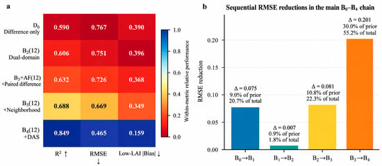
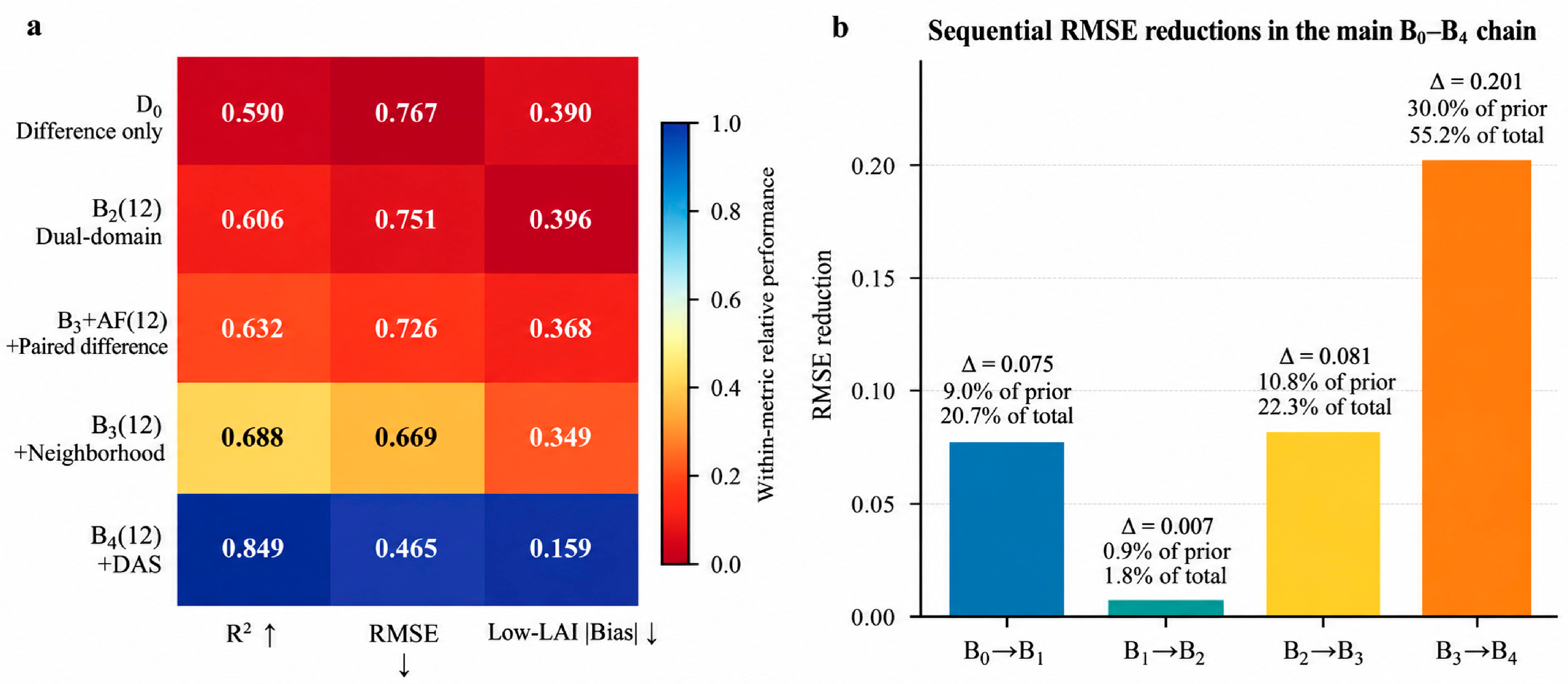
The difference-only diagnostic D0 achieved R2 = 0.590 and RMSE = 0.767. B2(12), which retained absolute information from both domains, achieved R2 = 0.606 and RMSE = 0.751. In this comparison, differences alone did not replace the predictive value of the absolute domain information. D0 and B2(12) are alternative representations rather than successive steps of a nested feature chain.
Under the common 12-feature upper limit, RMSE decreased from 0.751 for B2(12) to 0.726 for B2+ΔF(12), 0.669 for B3(12), and 0.465 for B4(12). The corresponding mean changes were −0.024953, −0.057431, and −0.203943 (Figure 6a). In the main B0–B4 sequence, RMSE reductions relative to the immediately preceding scheme were 0.075316 (B0 to B1), 0.006552 (B1 to B2), 0.081206 (B2 to B3), and 0.201308 (B3 to B4). These reductions corresponded to 9.03%, 0.86%, 10.80%, and 30.00% of the preceding RMSE, respectively (Figure 6b). Because the main schemes differ in input composition and maximum feature limits, these values are descriptive sequential changes rather than independent causal feature contributions.
Figure 6.
Feature-count controls and sequential RMSE summaries. (a) Performance of the separate D0 diagnostic and four controls with at most 12 selected features. Values are printed in each cell; colors are normalized within each metric and are not contribution percentages. Upward (↑) and downward (↓) arrows in (a) indicate that higher R2 values and lower RMSE or |Bias| values represent better performance, respectively. (b) RMSE reductions between adjacent main B0–B4 schemes. Each bar reports the reduction relative to the preceding scheme, its percentage of the preceding RMSE, and its share of the total B0–B4 RMSE decline. These quantities are descriptive and order-dependent because the main schemes differ in input composition and feature limits.
3.5. High-LAI Underestimation and Unseen-Date Prediction
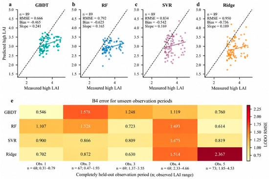
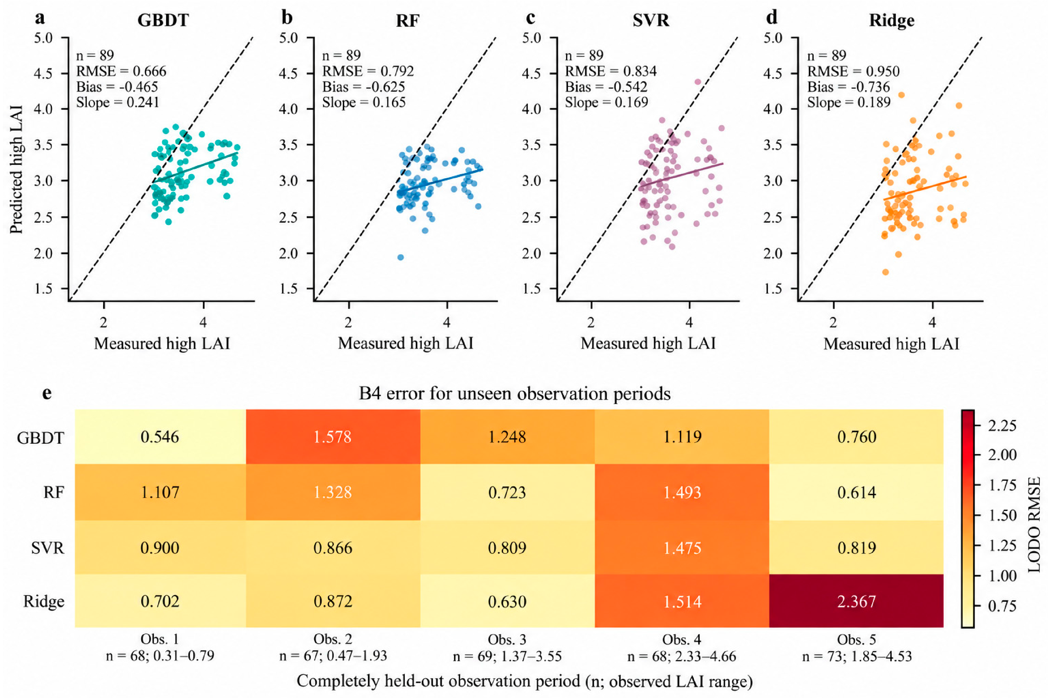
Although B4 markedly improved overall and low-LAI accuracy, high-LAI samples were consistently underestimated across the four regression models. The high-LAI RMSE values of GBDT, RF, SVR, and Ridge were 0.666, 0.792, 0.834, and 0.950, respectively. Their Bias values were −0.465, −0.625, −0.542, and −0.736, and their Slope values were 0.241, 0.165, 0.169, and 0.189, respectively (Figure 7a–d).
Figure 7.
High-LAI and unseen-date diagnostics. (a–d) Mean OOF predictions for 89 samples with measured LAI ≥ 3. Dashed lines show 1:1 agreement and solid lines show linear trends; panels report sample size, RMSE, Bias, and Slope. Conditional spatial-block slope bounds are provided in Supplementary Table S4. (e) B4 LODO RMSE by model and held-out date; labels give date-specific sample size and measured LAI range.
Unseen-date prediction produced substantial date-specific errors (Figure 7e). For GBDT B4, pooled LODO RMSE was 1.106, and R2 was negative within each held-out date. The second date had RMSE = 1.578. Replacing the pooled-training canopy threshold with the nearest training-date threshold reduced the mean of the five date-specific RMSEs only from 1.0499 to 1.0455. For the first date, fallback frequency decreased from 51/68 to 29/68 samples. Fewer fallback events therefore did not resolve the unseen-date prediction limitation. Pooled RMSE and the unweighted mean of date-specific RMSEs are distinct summaries.
4. Discussion
4.1. Effects of the Image Statistical Domain
The early observation date showed marked inter-domain contrast: about 30% of pixels were retained by the descriptive canopy mask, and mean |ΔNDVI| was 0.128. Low-LAI Bias decreased from 0.580 for B0 to 0.383 for B1. This comparison is consistent with a contribution from background screening, although it does not isolate every cause of error. Residue and soil can alter vegetation indices and early-stage LAI estimation [22,23]. Comparing two statistical domains within the same image window provides a direct way to assess this sensitivity.
The canopy domain does not mean complete background removal. Residue and soil may have similar reflectance patterns in the visible to near-infrared range, and these patterns are affected by moisture content [26]. The Otsu threshold can also be influenced by shadows, senescent leaves, and illumination changes. Therefore, the role of B1 is to shift the statistical center toward the green canopy, not to guarantee that all retained pixels are pure canopy pixels. The residue-soil-adjusted red-edge index can improve low-LAI estimation [24], and soil-adjusted vegetation indices reduce background effects from the perspectives of the soil line or brightness correction [40,41]. However, these indices are still calculated within a fixed image domain. The dual-domain design in this study further separates the question of which pixels are used for statistics from the question of which indices are calculated, allowing background correction to occur first at the level of the remote-sensing statistical domain.
Full-plot and canopy statistics were most similar at the third observation date, whereas their contrast increased again at the fourth. Such differences may reflect canopy cover, inter-row gaps, shadows, senescence, and background conditions. These alternatives were not separated experimentally. Soil and canopy properties can jointly influence spectral responses [25,27], so inter-domain contrasts should not be treated as a monotonic function of approximate DAS.
4.2. Paired Differences, Neighborhood Statistics, and DAS Play Different Roles
The fixed-capacity comparison supports a modest conditional improvement after adding paired-difference features to absolute dual-domain inputs. The differences explicitly represent contrasts between two statistical descriptions of the same window. They may simplify the representation available to a fitted model, but this comparison does not establish a distinct physical mechanism. Earlier maize studies similarly motivate examining combinations of spectral and spatial information through controlled comparisons [11,13].
Neighborhood statistics provided an additional improvement under the fixed-capacity comparison. Their variability measures summarize local reflectance heterogeneity rather than directly observing vertical canopy structure. The effect is conditional on the selected features, sample distribution, and validation design [19,44]. It should therefore be distinguished from evidence that the same features will improve prediction in new years or locations.
Approximate DAS provided a calendar-time reference that adjusted the prediction baseline across observation dates. In this statistical sense, it acted as a temporal constraint or date-conditioning variable; no explicit physiological trajectory or physical bound was imposed. Because the same five dates were represented in training and validation, DAS could partly identify observation date, and date-associated variation accounted for much of the overall B3-to-B4 improvement. The controlled B0–B4 comparisons still show how prediction changed among spectral input schemes under identical spatial folds. This distinction separates the comparative value of those schemes from the additional between-date adjustment supplied by approximate DAS.
4.3. Persistent High-LAI Underestimation
All four B4 models underestimated high LAI, with regression slopes ranging from 0.165 to 0.241. This shared behavior is consistent with limited spectral sensitivity, but it does not identify a unique cause. The high-LAI sample distribution, fixed hyperparameters, measurement uncertainty, and one-season design may also contribute. Vegetation-index saturation is a relevant explanation [30,31,35,39], rather than a mechanism proved by these comparisons.
Two-dimensional multispectral reflectance mainly describes the spectral response of the upper canopy surface and has limited sensitivity to vertical leaf distribution, canopy height, inter-layer occlusion, and ear-layer structure. A systematic review of spectral saturation in high-density vegetation reported that sensor band position, canopy structure, and observation mode jointly determine the saturation level, and recommended integrating airborne light detection and ranging (LiDAR), radar, or three-dimensional structural information [45]. Three-dimensional point clouds derived from UAV oblique imagery have been used to estimate maize LAI and canopy height simultaneously [46]. Compared with nadir orthomosaics, oblique photography can obtain more complete canopy-layer point clouds [47]. Canopy complexity metrics from airborne laser scanning (ALS) and unmanned aerial vehicle (UAV) stereo imagery can also serve as predictors of maize LAI [48]. Therefore, future work should introduce digital surface models (DSMs), digital terrain models (DTMs), canopy height models (CHMs), point-cloud height percentiles, canopy volume, or row-structure indicators into the existing dual-domain spectral representation to test whether three-dimensional canopy information can reduce high-LAI underestimation.
The present results motivate testing structural observations alongside the existing spectral representation. They do not demonstrate that two-dimensional imagery imposes an irreducible accuracy limit. Additional data and independently evaluated alternatives would be needed to distinguish sensitivity limitations from sampling, reference measurement, and model effects.
4.4. Validation Scope and Future Applications
Comparing four regression algorithms reduced reliance on a single model specification. Consistent directions of change across these algorithms support the reported scheme comparisons within this dataset, but do not isolate a causal feature effect. Fixed hyperparameters provide a common reference rather than an exhaustive search for each algorithm’s best performance [14,48].
Repeated spatial validation estimates performance at new sample locations on dates represented in training. It does not establish performance in independent fields, seasons, or unseen dates. Spatial grouping and buffer sensitivity reduce some concerns about close neighbors [28,42], but cannot establish the absence of residual spatial dependence. LODO additionally changes date coverage and the target spectral and LAI distributions. Its substantial date-specific biases should guide application scope rather than be obscured by pooled accuracy [43].
The farmer-managed setting spans management conditions encountered in local production, but incomplete field-level records of cultivar, planting density, row spacing, fertilization, irrigation, and crop protection limit management-specific interpretation. Sampling locations were generally selected anew across campaigns rather than maintained as permanent plots. Other uncertainties include canopy segmentation and the mismatch between instrument and image support areas. Approximate DAS provides a common calendar reference rather than verified crop age for each field. As a sensitivity check within this single season, replacing approximate DAS with cumulative growing degree days for the same five campaign dates produced nearly identical model behavior because both variables encoded the same date sequence. Growing degree days or observed phenological stages may become more informative across environments when reliable field-specific sowing dates, temperature records, and independent multi-year or multi-site observations are available [20,49].
5. Conclusions
This study provides a reproducible comparison of full-plot, canopy, paired-difference, neighborhood, and approximate-DAS inputs for summer maize LAI estimation under residue-mixed conditions. Spectral scheme comparisons and fixed-capacity controls support conditional benefits from changing the image representation. These findings apply to the sampled production-field conditions and the stated validation design.
Approximate DAS supplied a statistical time reference and accounted for much of the improvement across dates. The controlled comparisons still support relative differences among the spectral schemes under the stated spatial validation, while the time-baseline and residual diagnostics show that the B3-to-B4 gain was dominated by between-date adjustment.
High-LAI underestimation and unseen-date biases remained important limitations. The results support application to new locations under dates and production conditions represented in training. Further evaluation should combine field-level agronomic information, reliable developmental or thermal-time descriptors, and canopy structural observations across independent seasons and locations. Within its stated scope, the dual-domain framework offers a reproducible basis for comparing background screening, paired differences, and neighborhood information in farmer-managed maize fields.
Supplementary Materials
The following supporting information can be downloaded at: https://www.mdpi.com/article/10.3390/ai7100433/s1, Supplementary Methods S1: Feature selection and conditional uncertainty analysis; Table S1: Canopy fallback frequency; Table S2: Relative prediction errors; Table S3: Paired RMSE differences and conditional intervals; Table S4: High-LAI slope intervals.
Author Contributions
Conceptualization, X.H., C.Z. and Q.Q.; methodology, X.H. and C.Z.; software, C.Z.; validation, X.H., C.Z. and Q.Q.; formal analysis, X.H. and C.Z.; investigation, X.H., C.Z., Y.S., G.D., C.L., Z.W., L.H., Y.J. and X.Z.; resources, X.H. and Q.Q.; data curation, C.Z., Y.S., G.D., C.L., Z.W., L.H., Y.J. and X.Z.; writing—original draft preparation, X.H. and C.Z.; writing—review and editing, X.H., C.Z. and Q.Q.; visualization, C.Z.; supervision, X.H. and Q.Q.; project administration, X.H. and Q.Q.; funding acquisition, X.H. and Q.Q. All authors have read and agreed to the published version of the manuscript.
Funding
This research was funded by the Key Program of the Shandong Provincial Meteorological Bureau (grant numbers 2023sdqxz03, 2024sdqxm02) and the Shandong Provincial Natural Science Foundation (Grant No. ZR2024QD029, ZR2025QC1066).
Institutional Review Board Statement
Not applicable.
Informed Consent Statement
Not applicable.
Data Availability Statement
The data presented in this study are available from the corresponding author upon reasonable request.
Acknowledgments
The authors thank the students and professors who assisted with field sampling, UAV image acquisition and ground LAI measurements.
Conflicts of Interest
The authors declare no conflicts of interest.
Abbreviations
The following abbreviations are used in this manuscript:
| B0–B4 | progressive feature schemes |
| CV | cross-validation |
| DAS | approximate days after sowing from a common reference date |
| GBDT | gradient boosting decision tree |
| LAI | leaf area index |
| LODO | leave-one-date-out |
| MAE | mean absolute error |
| NDVI | normalized difference vegetation index |
| NIR | near-infrared |
| RF | random forest |
| RMSE | root mean square error |
| SAVI | soil-adjusted vegetation index |
| SVR | support vector regression |
| UAV | unmanned aerial vehicle |
| VI | vegetation index |
| WDRVI | wide dynamic range vegetation index |
References
- Fang, H.; Baret, F.; Plummer, S.; Schaepman-Strub, G. An Overview of Global Leaf Area Index (LAI): Methods, Products, Validation, and Applications. Rev. Geophys. 2019, 57, 739–799. [Google Scholar] [CrossRef] [Scilit]
- Breda, N.J.J. Ground-based measurements of leaf area index: A review of methods, instruments and current controversies. J. Exp. Bot. 2003, 54, 2403–2417. [Google Scholar] [CrossRef] [Scilit] [PubMed]
- Atzberger, C. Advances in Remote Sensing of Agriculture: Context Description, Existing Operational Monitoring Systems and Major Information Needs. Remote Sens. 2013, 5, 949–981, Correction in Remote Sens. 2013, 5, 4124. [Google Scholar] [CrossRef] [Scilit]
- Mulla, D.J. Twenty five years of remote sensing in precision agriculture: Key advances and remaining knowledge gaps. Biosyst. Eng. 2013, 114, 358–371. [Google Scholar] [CrossRef] [Scilit]
- Aasen, H.; Honkavaara, E.; Lucieer, A.; Zarco-Tejada, P.J. Quantitative Remote Sensing at Ultra-High Resolution with UAV Spectroscopy: A Review of Sensor Technology, Measurement Procedures, and Data Correction Workflows. Remote Sens. 2018, 10, 1091. [Google Scholar] [CrossRef] [Scilit]
- Maes, W.H.; Steppe, K. Perspectives for Remote Sensing with Unmanned Aerial Vehicles in Precision Agriculture. Trends Plant Sci. 2019, 24, 152–164. [Google Scholar] [CrossRef] [Scilit] [PubMed]
- Verrelst, J.; Camps-Valls, G.; Muñoz-Marí, J.; Rivera, J.P.; Veroustraete, F.; Clevers, J.G.P.W.; Moreno, J. Optical remote sensing and the retrieval of terrestrial vegetation bio-geophysical properties—A review. ISPRS J. Photogramm. Remote Sens. 2015, 108, 273–290. [Google Scholar] [CrossRef] [Scilit]
- Jacquemoud, S.; Verhoef, W.; Baret, F.; Bacour, C.; Zarco-Tejada, P.J.; Asner, G.P.; François, C.; Ustin, S.L. PROSPECT+SAIL models: A review of use for vegetation characterization. Remote Sens. Environ. 2009, 113, S56–S66. [Google Scholar] [CrossRef] [Scilit]
- Mananze, S.; Pôças, I.; Cunha, M. Retrieval of Maize Leaf Area Index Using Hyperspectral and Multispectral Data. Remote Sens. 2018, 10, 1942. [Google Scholar] [CrossRef] [Scilit]
- Chakhvashvili, E.; Siegmann, B.; Muller, O.; Verrelst, J.; Bendig, J.; Kraska, T.; Rascher, U. Retrieval of Crop Variables from Proximal Multispectral UAV Image Data Using PROSAIL in Maize Canopy. Remote Sens. 2022, 14, 1247. [Google Scholar] [CrossRef] [Scilit] [PubMed]
- Zhang, X.; Zhang, K.; Sun, Y.; Zhao, Y.; Zhuang, H.; Ban, W.; Chen, Y.; Fu, E.; Chen, S.; Liu, J.; et al. Combining Spectral and Texture Features of UAS-Based Multispectral Images for Maize Leaf Area Index Estimation. Remote Sens. 2022, 14, 331. [Google Scholar] [CrossRef] [Scilit]
- Buthelezi, S.; Mutanga, O.; Sibanda, M.; Odindi, J.; Clulow, A.D.; Chimonyo, V.G.P.; Mabhaudhi, T. Assessing the Prospects of Remote Sensing Maize Leaf Area Index Using UAV-Derived Multi-Spectral Data in Smallholder Farms across the Growing Season. Remote Sens. 2023, 15, 1597. [Google Scholar] [CrossRef] [Scilit]
- Ma, J.; Chen, P.; Wang, L. A Comparison of Different Data Fusion Strategies’ Effects on Maize Leaf Area Index Prediction Using Multisource Data from Unmanned Aerial Vehicles (UAVs). Drones 2023, 7, 605. [Google Scholar] [CrossRef] [Scilit]
- Guo, A.; Ye, H.; Huang, W.; Qian, B.; Wang, J.; Lan, Y.; Wang, S. Inversion of maize leaf area index from UAV hyperspectral and multispectral imagery. Comput. Electron. Agric. 2023, 212, 108020. [Google Scholar] [CrossRef] [Scilit]
- Friedman, J.H. Greedy function approximation: A gradient boosting machine. Ann. Stat. 2001, 29, 1189–1232. [Google Scholar] [CrossRef] [Scilit]
- Breiman, L. Random Forests. Mach. Learn. 2001, 45, 5–32. [Google Scholar] [CrossRef] [Scilit]
- Cortes, C.; Vapnik, V. Support-vector networks. Mach. Learn. 1995, 20, 273–297. [Google Scholar] [CrossRef] [Scilit]
- Hoerl, A.E.; Kennard, R.W. Ridge Regression: Biased Estimation for Nonorthogonal Problems. Technometrics 1970, 12, 55–67. [Google Scholar] [CrossRef]
- Li, H.; Huang, C.; Zhang, Y.; Li, S.; Liu, Y.; Yang, K.; Lu, J. Estimating Maize Leaf Area Index Using Multi-Source Features Derived from UAV Multispectral Imagery and Machine Learning Models. Plants 2025, 14, 3534. [Google Scholar] [CrossRef] [Scilit] [PubMed]
- Huang, W.; Liu, H.; Zhang, T.; Yang, L. Study on the Retrieval of Leaf Area Index for Summer Maize Based on Hyperspectral Data. AgriEngineering 2025, 7, 418. [Google Scholar] [CrossRef] [Scilit]
- Fu, W.; Chen, Z.; Cheng, Q.; Li, Y.; Zhai, W.; Ding, F.; Kuang, X.; Chen, D.; Duan, F. Maize Leaf Area Index Estimation Based on Machine Learning Algorithm and Computer Vision. Agriculture 2025, 15, 1272. [Google Scholar] [CrossRef] [Scilit]
- Zhao, D.; Yang, T.; An, S. Effects of crop residue cover resulting from tillage practices on LAI estimation of wheat canopies using remote sensing. Int. J. Appl. Earth Obs. Geoinf. 2012, 14, 169–177. [Google Scholar] [CrossRef] [Scilit]
- Liu, S.; Jin, X.; Bai, Y.; Wu, W.; Cui, N.; Cheng, M.; Liu, Y.; Meng, L.; Jia, X.; Nie, C.; et al. UAV multispectral images for accurate estimation of the maize LAI considering the effect of soil background. Int. J. Appl. Earth Obs. Geoinf. 2023, 121, 103383. [Google Scholar] [CrossRef] [Scilit]
- Li, W.; Li, D.; Liu, S.; Baret, F.; Ma, Z.; He, C.; Warner, T.A.; Guo, C.; Cheng, T.; Zhu, Y.; et al. RSARE: A physically-based vegetation index for estimating wheat green LAI to mitigate the impact of leaf chlorophyll content and residue-soil background. ISPRS J. Photogramm. Remote Sens. 2023, 200, 138–152. [Google Scholar] [CrossRef] [Scilit]
- Darvishzadeh, R.; Skidmore, A.; Atzberger, C.; van Wieren, S. Estimation of vegetation LAI from hyperspectral reflectance data: Effects of soil type and plant architecture. Int. J. Appl. Earth Obs. Geoinf. 2008, 10, 358–373. [Google Scholar] [CrossRef] [Scilit]
- Nagler, P.L.; Daughtry, C.S.T.; Goward, S.N. Plant Litter and Soil Reflectance. Remote Sens. Environ. 2000, 71, 207–215. [Google Scholar] [CrossRef] [Scilit]
- Raman, R.; Neely, H.L.; Rajan, N.; Siegfried, J.; Ibrahim, A.M.H.; Adams, C.B.; Hardin, R.G. Soil background effects on UAS and proximal remote sensing-derived vegetation indices. Agron. J. 2026, 118, e70281. [Google Scholar] [CrossRef] [Scilit]
- Roberts, D.R.; Bahn, V.; Ciuti, S.; Boyce, M.S.; Elith, J.; Guillera-Arroita, G.; Hauenstein, S.; Lahoz-Monfort, J.J.; Schröder, B.; Thuiller, W.; et al. Cross-validation strategies for data with temporal, spatial, hierarchical, or phylogenetic structure. Ecography 2017, 40, 913–929. [Google Scholar] [CrossRef] [Scilit]
- Otsu, N. A Threshold Selection Method from Gray-Level Histograms. IEEE Trans. Syst. Man Cybern. 1979, 9, 62–66. [Google Scholar] [CrossRef] [Scilit]
- Baret, F.; Guyot, G. Potentials and limits of vegetation indices for LAI and APAR assessment. Remote Sens. Environ. 1991, 35, 161–173. [Google Scholar] [CrossRef] [Scilit]
- Dong, T.; Liu, J.; Shang, J.; Qian, B.; Ma, B.; Kovacs, J.M.; Walters, D.; Jiao, X.; Geng, X.; Shi, Y. Assessment of red-edge vegetation indices for crop leaf area index estimation. Remote Sens. Environ. 2019, 222, 133–143. [Google Scholar] [CrossRef] [Scilit]
- Rondeaux, G.; Steven, M.; Baret, F. Optimization of soil-adjusted vegetation indices. Remote Sens. Environ. 1996, 55, 95–107. [Google Scholar] [CrossRef] [Scilit]
- Gitelson, A.A.; Kaufman, Y.J.; Merzlyak, M.N. Use of a green channel in remote sensing of global vegetation from EOS-MODIS. Remote Sens. Environ. 1996, 58, 289–298. [Google Scholar] [CrossRef] [Scilit]
- Jiang, Z.; Huete, A.; Didan, K.; Miura, T. Development of a two-band enhanced vegetation index without a blue band. Remote Sens. Environ. 2008, 112, 3833–3845. [Google Scholar] [CrossRef] [Scilit]
- Nguy-Robertson, A.; Gitelson, A.; Peng, Y.; Viña, A.; Arkebauer, T.; Rundquist, D. Green Leaf Area Index Estimation in Maize and Soybean: Combining Vegetation Indices to Achieve Maximal Sensitivity. Agron. J. 2012, 104, 1336–1347. [Google Scholar] [CrossRef] [Scilit]
- Dash, J.; Curran, P.J. The MERIS terrestrial chlorophyll index. Int. J. Remote Sens. 2004, 25, 5403–5413. [Google Scholar] [CrossRef] [Scilit]
- Gitelson, A.A. Wide Dynamic Range Vegetation Index for Remote Quantification of Biophysical Characteristics of Vegetation. J. Plant Physiol. 2004, 161, 165–173. [Google Scholar] [CrossRef] [Scilit] [PubMed]
- Haboudane, D.; Miller, J.R.; Tremblay, N.; Zarco-Tejada, P.J.; Dextraze, L. Integrated narrow-band vegetation indices for prediction of crop chlorophyll content for application to precision agriculture. Remote Sens. Environ. 2002, 81, 416–426. [Google Scholar] [CrossRef] [Scilit]
- Delegido, J.; Verrelst, J.; Meza, C.M.; Rivera, J.P.; Alonso, L.; Moreno, J. A red-edge spectral index for remote sensing estimation of green LAI over agroecosystems. Eur. J. Agron. 2013, 46, 42–52. [Google Scholar] [CrossRef] [Scilit]
- Qi, J.; Chehbouni, A.; Huete, A.R.; Kerr, Y.H.; Sorooshian, S. A modified soil adjusted vegetation index. Remote Sens. Environ. 1994, 48, 119–126. [Google Scholar] [CrossRef] [Scilit]
- Huete, A.R. A soil-adjusted vegetation index (SAVI). Remote Sens. Environ. 1988, 25, 295–309. [Google Scholar] [CrossRef] [Scilit]
- Valavi, R.; Elith, J.; Lahoz-Monfort, J.J.; Guillera-Arroita, G. blockCV: An R package for generating spatially or environmentally separated folds for k-fold cross-validation of species distribution models. Methods Ecol. Evol. 2019, 10, 225–232. [Google Scholar] [CrossRef] [Scilit]
- Meyer, H.; Pebesma, E. Predicting into unknown space? Estimating the area of applicability of spatial prediction models. Methods Ecol. Evol. 2021, 12, 1620–1633. [Google Scholar] [CrossRef] [Scilit]
- Zhang, J.; Cheng, J.; Liu, C.; Wu, Q.; Xiong, S.; Yang, H.; Chang, S.; Fu, Y.; Yang, M.; Zhang, S.; et al. Enhanced Crop Leaf Area Index Estimation via Random Forest Regression: Bayesian Optimization and Feature Selection Approach. Remote Sens. 2024, 16, 3917. [Google Scholar] [CrossRef] [Scilit]
- Mutanga, O.; Masenyama, A.; Sibanda, M. Spectral saturation in the remote sensing of high-density vegetation traits: A systematic review of progress, challenges, and prospects. ISPRS J. Photogramm. Remote Sens. 2023, 198, 297–309. [Google Scholar] [CrossRef] [Scilit]
- Li, M.; Shamshiri, R.R.; Schirrmann, M.; Weltzien, C.; Shafian, S.; Laursen, M.S. UAV Oblique Imagery with an Adaptive Micro-Terrain Model for Estimation of Leaf Area Index and Height of Maize Canopy from 3D Point Clouds. Remote Sens. 2022, 14, 585. [Google Scholar] [CrossRef] [Scilit]
- Che, Y.; Wang, Q.; Xie, Z.; Zhou, L.; Li, S.; Hui, F.; Wang, X.; Li, B.; Ma, Y. Estimation of maize plant height and leaf area index dynamics using an unmanned aerial vehicle with oblique and nadir photography. Ann. Bot. 2020, 126, 765–773. [Google Scholar] [CrossRef] [Scilit] [PubMed]
- Li, W.; Niu, Z.; Chen, H.; Li, D. Characterizing canopy structural complexity for the estimation of maize LAI based on ALS data and UAV stereo images. Int. J. Remote Sens. 2017, 38, 2106–2116. [Google Scholar] [CrossRef] [Scilit]
- Walne, C.H.; Reddy, K.R. Temperature Effects on the Shoot and Root Growth, Development, and Biomass Accumulation of Corn (Zea mays L.). Agriculture 2022, 12, 443. [Google Scholar] [CrossRef] [Scilit]

Disclaimer/Publisher’s Note: The statements, opinions and data contained in all publications are solely those of the individual author(s) and contributor(s) and not of MDPI and/or the editor(s). MDPI and/or the editor(s) disclaim responsibility for any injury to people or property resulting from any ideas, methods, instructions or products referred to in the content. |
© 2026 by the authors. Licensee MDPI, Basel, Switzerland. This article is an open access article distributed under the terms and conditions of the Creative Commons Attribution (CC BY) license.