Remote Sensing Scene Classification via Multi-Feature Fusion Based on Discriminative Multiple Canonical Correlation Analysis

Abstract

Scene classification in remote sensing images is one of the urgent tasks that requires an improvement in recognition accuracy due to complex spatial structures and high inter-class similarity. Although feature extraction using convolutional neural networks provides high efficiency, combining deep features obtained from different architectures in a semantically consistent manner remains an important scientific problem. In this study, a DMCCA + SVM model is proposed, in which Discriminative Multiple Canonical Correlation Analysis (DMCCA) is applied to fuse multi-source deep features, and final classification is performed using a Support Vector Machine (SVM). Unlike conventional fusion methods, DMCCA projects heterogeneous features into a unified low-dimensional latent space by maximizing within-class correlation and minimizing between-class correlation, resulting in a more separable and compact feature space. The proposed approach was evaluated on three widely used benchmark datasets—NWPU-RESISC45, AID, and PatternNet—and achieved accuracy scores of 92.75%, 93.92%, and 99.35%, respectively. The results showed that the model outperforms modern individual CNN architectures. Additionally, the model’s stability and generalization capability were confirmed through K-fold cross-validation. Overall, the proposed DMCCA + SVM model was experimentally validated as an effective and reliable solution for high-accuracy classification of remote sensing scenes.

1. Introduction

As the scale and complexity of global remote sensing (RS) images continue to grow, processing and analysis have become increasingly complex. RS images provide a key source of information in applications related to meteorology, mapping, monitoring for urban change, and agricultural monitoring [1,2,3,4]. Their very high spatial resolution makes them useful for automatically classifying scenes. However, despite the high resolution, the task is made much harder by the fact that image structures are complex, there are many objects in a single frame, classes are semantically similar, lighting conditions change, and geometric positions and structures are different [1]. Consequently, the creation of systems proficient in accurately and reliably classifying scenes in remote sensing images continues to be a significant scientific challenge. Recent large-scale operational monitoring systems further emphasize this challenge. For example, ref. [5] proposed a global land change monitoring framework that rapidly analyzes high-resolution remote sensing imagery to track vegetation loss and land cover dynamics at a planetary scale, highlighting the growing demand for accurate and robust remote sensing image analysis methods.

Deep learning technologies, especially convolutional neural networks (CNNs), have done very well in image analysis in the last few years, showing that they are better than traditional machine learning methods [6,7]. CNNs’ ability to learn features hierarchically makes it possible to effectively classify complex scenes in RS images. But using just one CNN architecture might not work well for extracting features from all types of RS images. Different CNN models, like ResNet18, DenseNet121, VGG16, EfficientNetB1, and AlexNet, have different structures and ways of learning that encode low-, mid-, and high-level abstract features in different ways. From this point of view, the integration of the features of various CNN models (functional fusion) can improve the overall classification performance [8,9,10]. Recently, foundation model-based approaches have also been explored for remote sensing image analysis, particularly in the context of semantic change detection. For instance, in [11], leveraged large vision–language models such as SAM and CLIP to move from binary to semantic change detection, demonstrating the potential of high-level semantic representations, albeit at the cost of increased model complexity and computational requirements. This approach uses the strengths of each model to create a richer and more semantic representation of images [12].

In recent years, several studies have addressed remote sensing scene classification using a two-stage strategy, where deep neural networks are first employed for feature extraction, followed by classification using traditional machine learning models. For instance, in [13], deep features extracted from different layers of CNN architectures were classified using an SVM, achieving results competitive with state-of-the-art end-to-end approaches. Similarly, ref. [14] proposed a method that combines features extracted via an Attention U-Net architecture with an XGBoost classifier; by emphasizing informative regions through attention mechanisms and incorporating contextual information, this approach achieved an accuracy of 92.67%. Recent comprehensive reviews further confirm the effectiveness of such two-stage paradigms in remote sensing applications, particularly for high-dimensional multisource data, where deep feature extraction followed by traditional machine learning classifiers offers a robust and computationally efficient solution [15].

The two-stage paradigm offers several practical and computational advantages. First, advanced deep architectures (e.g., ResNet, U-Net, TransUNet) can be utilized in a pre-trained manner as powerful feature extractors, while only lightweight classifiers such as SVM or XGBoost need to be trained. This significantly reduces computational cost and mitigates overfitting, especially when training data are limited. Moreover, classifiers such as SVM are well known for their ability to handle high-dimensional feature spaces effectively, even with relatively small training sets.

Therefore, for remote sensing scene classification tasks characterized by high intra-class variability, limited labeled data, and large feature dimensionality, the two-stage framework represents a practical and efficient alternative to fully end-to-end fusion networks, offering a favorable trade-off between performance, robustness, and computational complexity.

The feature fusion can take place at three main levels: data integration at the pixel level, combination at the feature level of learned representations, and decision-level fusion of classifier output. Functional fusion is often regarded as superior because it preserves discriminatory structures and enables more direct control of unified functional vectors. However, each fusion level has its own advantages and can be effective based on the research objectives and types of data used [16]. However, feature vectors derived from different CNN architectures are usually high-dimensional and may contain redundant information, complicating computer processing and potentially causing “dimensionalization curse” problems. So, we need to use efficient fusion mechanisms and dimensionality reduction techniques [8]. Canonical Correlation Analysis (CCA) and its multi-set variant (MCCA) are widely used to identify linear relationships between multiple feature sets and project them into a lower-dimensional space [9,17].

In recent years, the Discriminative Multiple Canonical Correlation Analysis (DMCCA) method has been proposed, enabling the extraction of more precise and discriminative information from multiple feature sets [18]. DMCCA is designed not only to maximize the correlation between feature sets but also to enhance within-class correlation and reduce between-class correlation, thereby identifying projection directions that improve classification performance [18,19]. Thus, combining the rich information content of features extracted from CNNs with the discriminative capabilities of DMCCA significantly increases the accuracy of RS image classification.

The main contributions of this work can be summarized as follows:

• An alternative DMCCA-based feature fusion approach for remote sensing scene classification is proposed. Unlike conventional fusion strategies such as feature concatenation, averaging, or attention-based mechanisms, the proposed approach employs DMCCA to integrate heterogeneous deep features into a unified low-dimensional latent space that enhances within-class correlation and suppresses between-class correlation.
• Systematic integration of heterogeneous CNN representations is achieved without additional trainable fusion modules. Deep features extracted from architecturally diverse CNN backbones (ResNet18, DenseNet121, and VGG16) are fused at the feature level using a statistically grounded discriminative correlation framework, avoiding the complexity and high data requirements of attention- or Transformer-based fusion networks.
• A lightweight and effective two-stage classification scheme is established. The proposed DMCCA + SVM approach decouples feature learning and classification by combining fine-tuned CNN feature extractors with a robust SVM classifier, making it well suited for remote sensing scenarios involving high-dimensional features and limited labeled data.
• Comprehensive experimental validation demonstrates effectiveness, robustness, and stability. Extensive experiments on three benchmark datasets (NWPU-RESISC45, AID, and PatternNet) show consistent performance improvements over individual CNN models across different training ratios. Robustness is further confirmed through 5-fold cross-validation, random splits, statistical reliability analysis (standard deviation and 95% confidence intervals), and qualitative visualization using t-SNE and UMAP. In addition, this study provides an empirical evaluation of DMCCA in the context of remote sensing scene classification, extending its application beyond previously explored domains.

Based on the above motivations, this work investigates a two-stage scene classification approach that combines deep CNN feature extraction with discriminative correlation-based fusion and SVM classification.

2. Related Works

Recently, scene classification in remote sensing images (Remote Sensing Scene Classification—RSSC) has become an area of extensive research with many deep learning models. Prior methods use traditional descriptors GLCM, LBP, SIFT, and HOG [1], which represent specific scenes to extract spatial and texture-based features. But these methods did not give a high-level semantic representation and were not very accurate in complicated scenes. So, the creation of deep learning models, especially CNN architectures, has been a big step forward in scene classification [20].

Models such as ResNet, DenseNet, VGG, EfficientNet, and AlexNet have enabled deep learning of complex structures through convolutional layers [21,22].

In particular, fine-tuning pre-trained models on large datasets such as ImageNet using transfer learning has demonstrated high effectiveness in RS image analysis [23,24]. Nevertheless, since each CNN model is sensitive only to certain aspects of the data, researchers have sought to improve classification accuracy by fusing features extracted from multiple sources. Feature fusion approaches make it possible to integrate various contextual and semantic information within a scene. Among these approaches, methods based on convolutional layer operations such as addition, concatenation, attention mechanisms [19,25,26], and statistical techniques are widely used.

Among statistical approaches, CCA [27] and its extensions, such as Multiple CCA (MCCA) [28], aim to identify maximum correlations between multi-source features. However, since these methods are based on linear projections, they are not sufficiently effective for deeply learned (deep) features. To address this issue, Deep CCA (DCCA) [29] was proposed, which enhances inter-modality correlations through nonlinear projections implemented by neural networks. But DCCA does not look at how similar things are within a class or how separate things are between classes. Discriminative MCCA (DMCCA) [19], conversely, addresses this limitation by projecting multiple feature sets into a unified discriminative space that enhances within-class correlation while diminishing between-class correlation.

In recent years, deep learning-based approaches for feature fusion from multimodal data have attracted considerable attention. Transformer architectures and attention mechanisms are particularly distinguished by their effectiveness in modeling long-range dependencies. By relying solely on attention mechanisms, Transformers eliminate the need for convolutional and recurrent layers, thereby enabling the capture of complex long-distance relationships within data.

In the remote sensing domain, for example, ref. [30] proposed the TRS model, which replaces the final convolutional blocks of the ResNet architecture with multi-head self-attention layers and incorporates a series of Transformer encoders. In this approach, convolutional operations are entirely replaced by attention layers, resulting in a significant improvement in classification accuracy. Similarly, ref. [29] introduced the SAFF (Self-Attention-based Feature Fusion) method, in which feature maps extracted by CNNs are adaptively refined using spatial and channel-wise attention mechanisms, allowing sufficient emphasis to be placed even on rare objects.

However, attention- and Transformer-based approaches typically require large volumes of training data and introduce additional trainable parameters. In contrast, the DMCCA-based feature fusion approach enables the effective integration of features extracted from different CNN models into a discriminative latent space without requiring complex retraining of deep architectures. Consequently, DMCCA represents a computationally lighter and practically efficient alternative for real-world remote sensing applications.

Other methods that have been suggested include self-attention [29], hierarchical fusion [31], and ensemble learning [32]. These methods use features gained from CNN models and employ a variety of statistical operators to fuse them. By fusing features that represent different types of context, these methods improve the accuracy of the classifier. Additionally, multi-feature fusion, or fusing features that come from different layers of flow network models, has been suggested as a productive avenue for analyzing remote sensing images [33,34,35,36]. The studies referenced discuss how semantic features from deeper layers of CNN models can be useful during the intermediate or late stages of fusion.

The past work shows that combining the features from the CNNs with statistics—especially with discriminatively correlated features through DMCCA—can improve extremely well in terms of accuracy, and help with robustness in classifying scene types. However, DMCCA has mainly been applied to biometric authentication, audio-visual fusion, and medical imaging, and has not been fully explored in visual classification tasks, including remote sensing scene classification. We draw motivation from this issue to implement the new study.

3. Methods

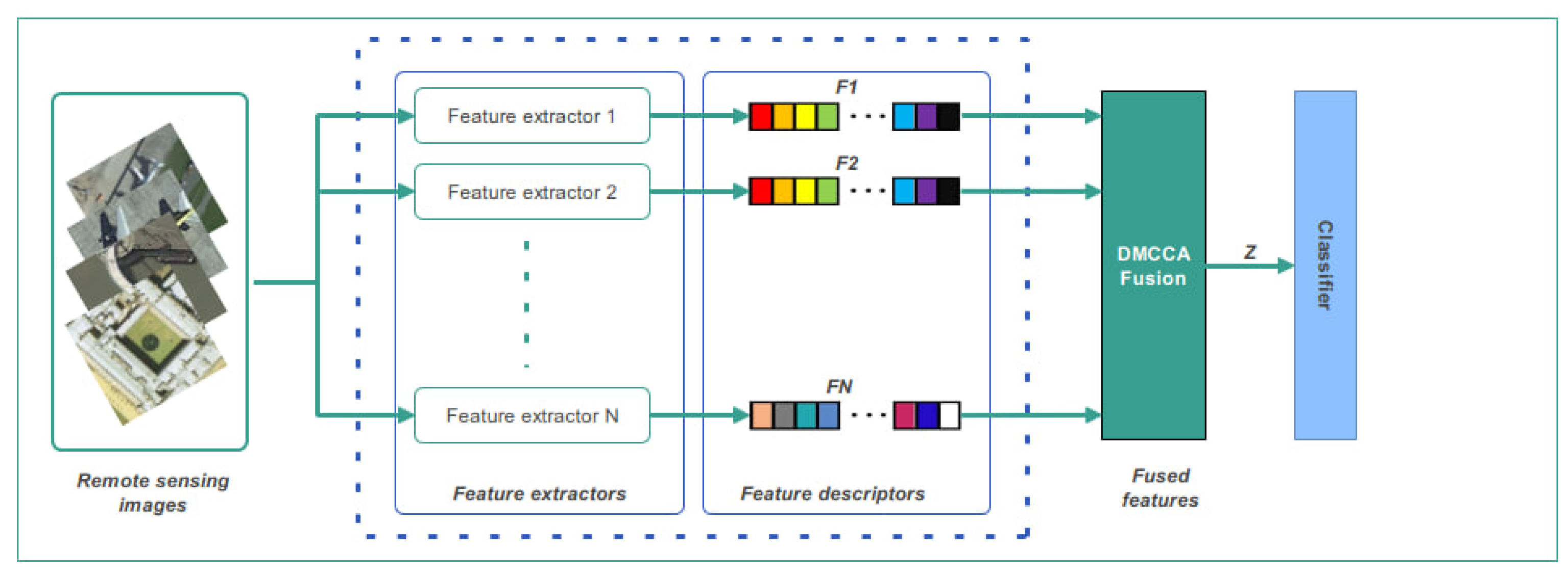
This research introduces a DMCCA-based approach aimed at enhancing scene classification precision in remote sensing images by combining features from multiple sources within deep learning. The core idea of the suggested method is to transform features obtained from different CNNs into a unified latent space and refine them while preserving their distinguishing characteristics. Figure 1 shows all the steps of the proposed approach and how they are related to each other in a diagram.

In the first step, transfer learning is used to use multiple pre-trained CNN models, such as ResNet18, DenseNet121, and VGG16, to get features from images. Convolutional layers, ReLU activation functions, pooling layers, and fully connected layers make up these models. They progressively capture characteristics at various levels of abstraction. The lower layers reveal fundamental features such as shape and texture, while the upper layers present features that are rich in meaning and semantics.

Each model has been trained on the ImageNet dataset before, which helps them learn general visual structures better. Instead of retraining these models, they are only used as feature extractors to quickly get high-level discriminative features from RS scenes.

In the next step, DMCCA aligns the feature vectors from different CNN models in a common latent space, making sure that the coordinates and correlations are the same. This step makes the connections between multi-source features stronger and makes it easier to accurately separate target scene classes. In the last step, a regular classifier, like an SVM, is used to sort the combined features.

3.1. Feature Extraction from Images Using CNN

In this study, multiple pre-trained CNNs were utilized for deep feature extraction in the task of RS scene classification. CNN architectures consist of convolutional layers, activation functions (e.g., ReLU), pooling layers, and final fully connected layers, through which features at different abstraction levels are progressively extracted from images. The lower layers identify low-level features such as structure and texture, while the higher layers represent semantic (meaningful) features.

In the research, CNN models such as ResNet18, DenseNet121, and VGG16 were employed as feature extraction tools. All of these models were pre-trained on the ImageNet dataset. Since ImageNet contains millions of images and over 1000 object classes, these models are capable of effectively learning general visual structures. Through the mechanism of transfer learning, they can be successfully adapted to RS images as well. In particular, using them as feature extractors without retraining leads to high performance.

Below is a brief description of the CNN models used for feature extraction in this study:

ResNet18. Proposed in 2015 to improve the training efficiency of deep convolutional neural networks, this model is based on the concept of residual connections (shortcut connections) [37,38]. These connections represent the output feature map by directly adding it to the input signal:

$$H\left(x\right) = F(x) + x$$

This approach reduces the vanishing gradient problem and ensures stable training even in very deep architectures. The ResNet18 model consists of 18 layers and takes an image of size 224 × 224 as input. The model gradually extracts features through four residual blocks and produces a 512-dimensional abstract feature vector at the output. Therefore, the ResNet18 architecture is considered a deep yet lightweight and efficient feature extraction model, widely used in various fields such as classification and object detection [37].

DenseNet121. Proposed in 2017 to enhance information flow in deep convolutional networks and reduce the number of parameters, this is an efficient architecture [39]. The main idea of the model is to introduce a densely connected structure (dense connectivity) between layers—that is, each layer receives as input the outputs of all preceding layers:

$$x_l ={ H}_l\left(\left[x_0,x_1,\dots ,x_{l\text{-}1}\right]\right)$$

where $\left[x_0,x_1,\dots ,x_{l\text{-}1}\right]$—is the concatenated representation of the outputs from all preceding layers. Such a densely connected architecture enables feature reuse, ensures stable gradient propagation, and accelerates the training process. The DenseNet121 model consists of 121 layers, composed of four Dense Blocks and intermediate Transition layers. The model takes an image that is $224 \times 224$ pixels and gives back a rich, multi-level, and detailed 1024-dimensional feature set [39].

VGG16. This model was conceived in 2014 to establish a clear and efficient structure for deep convolutional neural networks. It proceeds by stacking small ($3 \times 3$) convolutional filters to promote depth, which allows the network to identify complex, high-level features. The VGG16 model is made up of 16 layers, takes in images of $224 \times 224$ pixels, and outputs a feature vector of 512 pixels. Because of the closeness of its layers and its simplicity, it is a great way of extracting deep features for classifying images and performing many tasks in remote sensing (RS). In the first part of the investigation, fresh images sourced from RS are placed into the ResNet18, DenseNet121, and VGG16 models, which were trained using the ImageNet dataset. All three models are used in a transfer learning manner, taking advantage of the parameters of the pre-trained models to adapt the training process using RS images.

In the second part of the study, the selected models’ feature extraction portions are used to obtain deep semantic features from the image. These features are high-level representations of features that are made in the convolutional layers of each model. They are the main input data for the next steps of fusion and classification. You can write the process down in math like this:

$$\begin{gathered} F_1 = f_{\mathrm{ResNet}18}\left(X\right), \\ {F}_2 ={ f}_{\mathrm{DensNet}121}\left(X\right), \\ {F}_3 = f_{\mathrm{VGG}16}\left(X\right), \end{gathered}$$

where $X\in R^{H\times W\times C}$ is the input image, $f_{\mathrm{ResNet}18}, f_{\mathrm{DensNet}121},{ f}_{\mathrm{VGG}16}$—are the feature extraction functions of the corresponding CNN models, and $F_1,{ F}_2,{ F}_3$—are the feature vectors that each model gives us. In this way, each model makes its own vector representation that shows different levels of the image’s spectral, spatial, and semantic features.

3.2. Feature Fusion Using DMCCA

When dealing with data from more than one source or dimension, it is important to be able to combine features from different sources in a useful way. Feature fusion can help the model generalize better, make more accurate classifications, and find hidden relationships in the data. To do this, a number of statistical and deep learning-based methods have been made. Among them, CCA, DCCA, MCCA, and DMCCA play significant roles. While CCA and DCCA methods are designed for only two feature vectors, MCCA and DMCCA can be applied to fuse multiple feature vectors. In the MCCA method, only correlation analysis between feature vectors is performed without considering inter-class differences. In contrast, the DMCCA method takes inter-class differences into account when combining multiple features. Feature fusion performed using DMCCA has demonstrated high accuracy in scene classification of RS images. Therefore, in this study, the features $F_1$,${ F}_2$, and $F_3$ extracted from multiple deep CNN models are fused using DMCCA.

Let us assume that a dataset with $c$ classes is given. From this dataset, $N$ descriptors $F_1\in R^{m_1},F_2\in R^{m_2},\cdots {,F}_N\in R^{m_N}$ are constructed, where the total feature dimension is $Q = m_1+m_2+\cdots +m_N$.

The DMCCA approach aims to integrate information by maximizing the within-class correlation and minimizing the between-class correlation. To achieve this, the following projection vectors are determined:

$$\omega = {[{{\omega }_1}^T,{ {\omega }_2}^T,\cdots ,{{\omega }_N}^T]}^T, {\omega }_1\in R^{m_1\times Q},{\omega }_2\in R^{m_2\times Q},\cdots ,{\omega }_N\in R^{m_N\times Q}.$$

The DMCCA problem is formulated as the following optimization task:

$$\underset{{\omega }_1,{\omega }_2,\cdots ,{\omega }_N}{\mathrm{argmax}}\rho = {\displaystyle \frac{1}{N(N\text{-}1)}}{\sum }_{k=1}^N{\sum }_{\begin{array}{c}m=1\\ m\ne k\end{array}}^N {\omega }_k^T{C}_{F_k{F}_m}^{\sim }{\omega }_m,$$

(1)

where $C_{F_k{F}_m}^{\sim } ={ C}_{w_{F_k{F}_m}} \text{-} \delta C_{b_{F_k{F}_m}}(\delta > 0)$—is the improved covariance matrix, where $\delta$ is the regularization coefficient that controls the balance between within-class and between-class correlations. The regularization parameter $\delta$ is introduced to ensure numerical stability in the generalized eigenvalue problem, particularly when handling high-dimensional feature spaces and limited training samples. In all experiments, $\delta$ was fixed to a small constant value ($\delta ={ 10}^{-6}$), which is commonly adopted in discriminative subspace learning methods. We observed that the model performance remained stable within a reasonable range of $\delta$, indicating low sensitivity to this parameter. $C_{F_k{F}_k}$ represents the covariance (or variance) matrix of the descriptor $F_k$, which is defined as follows:

$$C_{F_k{F}_k} ={ F}_k{F_k}^T.$$

$C_{w_{F_k{F}_m}}$ and $C_{b_{F_k{F}_m}}$ denote the within-class and between-class correlation matrices, respectively, of the $N$ descriptors.

The optimization problem (1) is solved under the following constraint:

$${\sum }_{k=1}^N {\omega }_k^T{C}_{F_k{F}_k}{\omega }_k = N$$

(2)

This constraint maintains the balance of the magnitudes (norms) of all projection vectors in the model and ensures that each descriptor contributes equally to the overall projection process. In this way, it prevents excessive dominance or suppression of features from different sources and guarantees stable results during the optimization process. $C_{w_{F_k{F}_m}}$ and $C_{b_{F_k{F}_m}}$ can be explicitly expressed using the following formulas:

$$C_{w_{F_k{F}_m}} = F_{k}A{F}_m^T.$$

(3)

$$C_{b_{F_k{F}_m}}= \text{-}{F}_{k}A{F}_m^T.$$

(4)

$$\mathrm{A}=\left(\begin{array}{ccc}{H}_{n_{i1}\times n_{i1}}& \cdots & 0\\ ⋮& H_{n_{\mathit{il}}\times n_{\mathit{il}}}& ⋮\\ 0& \cdots & H_{n_{\mathit{ic}}\times n_{\mathit{ic}}}\end{array}\right).$$

(5)

where $n_{\mathit{il}}$ denotes the number of samples of the descriptor $F_i$ in class $l$, and $H_{n_{\mathit{il}}\times n_{\mathit{il}}}$ is an $n_{\mathit{il}} \times n_{\mathit{il}}$ matrix in which all elements are ones.

In other words, matrix $A$ has a block-diagonal structure according to the classes, where each block represents the internal relationships among samples within the corresponding class. Through this structure, the matrices $C_{w_{F_k{F}_m}}$ and $C_{b_{F_k{F}_m}}$ enable the computation of within-class and between-class correlations between descriptors.

If expressions (3) and (4) are substituted into (1), the DMCCA optimization problem takes the following form:

$$\underset{{\omega }_1,{\omega }_2,\cdots ,{\omega }_N}{\arg \max }\rho ={\displaystyle \frac{1}{N\left(N\text{-}1\right)}}{\sum }_{k=1}^N{\sum }_{\begin{array}{c}m=1\\ m\ne k\end{array}}^N {\omega }_k^T{C}_{F_k{F}_m}^{\sim }{\omega }_m ={\displaystyle \frac{1+\delta }{N\left(N\text{-}1\right)}}{\sum }_{k=1}^N{\sum }_{\begin{array}{c}m=1\\ m\ne k\end{array}}^N{\omega }_k^T{F}_{k}A{F}_m^T{\omega }_m .$$

(6)

The optimization is performed subject to the following constraint:

$${\sum }_{k=1}^N {\omega }_k^T{C}_{F_k{F}_k}{\omega }_k=N.$$

(7)

Using expressions (6) and (7), the Lagrange multiplier method is applied, i.e., the constraint is added to the optimization function, and the derivatives of the resulting Lagrangian function are set to zero. As a result, a generalized eigenvalue problem that determines the projection vectors is obtained:

$$\begin{gathered} {\displaystyle \frac{1+\delta }{N\text{-}1}}\left(\begin{array}{ccccc}0& F_{1}A{F}_2^T& F_{1}A{F}_3^T& \dots & F_{1}A{F}_N^T\\ F_{2}A{F}_1^T& 0& F_{2}A{F}_3^T& \dots & F_{2}A{F}_N^T\\ F_{3}A{F}_1^T& F_{3}A{F}_2^T& 0& \dots & F_{3}A{F}_N^T\\ & ⋮& & & \\ F_{N}A{F}_1^T& F_{N}A{F}_2^T& F_{N}A{F}_3^T& \dots & 0\end{array}\right)\omega = \\ =\rho \left(\begin{array}{ccccc}{F}_1{F}_1^T& 0& 0& \dots & 0\\ 0& F_2{F}_2^T& 0& \dots & 0\\ 0& 0& F_3{F}_3^T& \dots & 0\\ & ⋮& & & \\ 0& 0& 0& \dots & F_N{F}_N^T\end{array}\right)\mathsf{\omega } \end{gathered}$$

(8)

By solving this equation, the optimal projection vectors for each descriptor in the DMCCA model are obtained. The canonical form of Equation (8) can be expressed as follows:

$${\displaystyle \frac{1+\delta }{N\text{-}1}}\left(C\text{-}D\right)\omega =\rho D\omega$$

(9)

where

$$\mathrm{C}=\left(\begin{array}{ccccc}{F}_1{F}_1^T& F_{1}A{F}_2^T& F_{1}A{F}_3^T& \dots & F_{1}A{F}_N^T\\ F_{2}A{F}_1^T& F_2{F}_2^T& F_{2}A{F}_3^T& \dots & F_{2}A{F}_N^T\\ F_{3}A{F}_1^T& F_{3}A{F}_2^T& F_3{F}_3^T& \dots & F_{3}A{F}_N^T\\ & ⋮& & & \\ F_{N}A{F}_1^T& F_{N}A{F}_2^T& F_{N}A{F}_3^T& \dots & F_N{F}_N^T\end{array}\right)$$

(10)

$$\mathrm{D}=\left(\begin{array}{ccccc}{F}_1{F}_1^T& 0& 0& \dots & 0\\ 0& F_2{F}_2^T& 0& \dots & 0\\ 0& 0& F_3{F}_3^T& \dots & 0\\ & ⋮& & & \\ 0& 0& 0& \dots & F_N{F}_N^T\end{array}\right)$$

(11)

$$\mathrm{C}\text{-}D=\left(\begin{array}{ccccc}0& F_{1}A{F}_2^T& F_{1}A{F}_3^T& \dots & F_{1}A{F}_N^T\\ F_{2}A{F}_1^T& 0& F_{2}A{F}_3^T& \dots & F_{2}A{F}_N^T\\ F_{3}A{F}_1^T& F_{3}A{F}_2^T& 0& \dots & F_{3}A{F}_N^T\\ & ⋮& & & \\ F_{N}A{F}_1^T& F_{N}A{F}_2^T& F_{N}A{F}_3^T& \dots & 0\end{array}\right)$$

(12)

$$\mathsf{\omega }={\left[{\omega }_1^T,{\omega }_2^T,\cdots {\omega }_N^T\right]}^T$$

(13)

Since $\frac{1+\delta }{N\text{-}1}$ is a constant and does not affect the projection matrix $\omega$, we define ${\rho }^{\prime }=\frac{N\text{-}1}{1+\delta }\rho$, and rewrite Equation (9) as follows:

$$\left(C\text{-}D\right)\omega ={\rho }^{\prime }D\omega$$

(14)

Through mathematical transformation, Equation (9) can be rewritten in the following form:

$$\begin{array}{cc}& F_{1}A{F}_2^T{\omega }_2+F_{1}A{F}_3^T{\omega }_3+\cdots +F_{1}A{F}_N^T{\omega }_N={\rho }^{\prime }{F}_1{\mathrm{F}}_1^{\mathrm{T}}{\omega }_1\\ & F_{2}A{F}_1^T{\omega }_1+F_{2}A{F}_3^T{\omega }_3+\cdots +F_{2}A{F}_N^T{\omega }_N={\rho }^{\prime }{F}_2{F}_2^T{\omega }_2\\ & ⋮\\ & F_{N}A{F}_1^T{\omega }_1+F_{N}A{F}_2^T{\omega }_2+\cdots +F_{N}A{F}_{N\text{-}1}^T{\omega }_{N\text{-}1}={\rho }^{\prime }{F}_N{F}_N^T{\omega }_N\end{array}$$

(15)

In evaluating the relationship between within-class and between-class correlation matrices, the value of ${\rho }^{\prime }$ plays a crucial role. If ${\rho }^{\prime }$ is greater than zero, the projection vector $\omega$ enhances recognition accuracy in classification. However, if ${\rho }^{\prime }$ is zero or negative, the vector $\omega$ reduces recognition accuracy in classification. As a solution, the eigenvectors corresponding to the $d$ largest positive eigenvalues in Equation (9) are selected.

Usually, the computation of projection vectors depends on extracting discriminative features using algebraic methods, which can be time-consuming. If the rank of the eigenmatrix is very high, calculating its eigenvalues and eigenvectors requires significant computational time. To efficiently address this issue, an important property of DMCCA has been established—namely, the dimensionality $d$ of the fused features corresponding to optimal recognition accuracy is less than or equal to the number of classes $c$:

$$d \le c$$

(16)

According to the theoretical formulation of DMCCA, the dimensionality of the fused latent space is bounded by the number of classes, i.e., $d \le c$. In our experiments, we set $d=c$ for all datasets, as this choice provided a compact yet sufficiently discriminative representation without introducing redundant dimensions. Preliminary experiments with smaller values of $d$ ($d < c$) resulted in a gradual degradation of classification performance, while increasing $d$ beyond $c$ did not yield additional performance gains. These observations empirically support the theoretical bound and justify the choice of $d=c$ in practice.

The following expression is used to fuse the descriptors:

$$Y_k={\omega }_k^T{F}_k , k=1,2,\dots ,N$$

(17)

$$\mathrm{Z}={\left[Y_1^T,Y_2^T,\cdots ,Y_N^T\right]}^{\mathrm{T}}\in R^{\mathit{dN}}$$

(18)

From a theoretical perspective, the optimal projection dimensionality of DMCCA is bounded by the number of classes ($d \le c$), which leads to an effective computational complexity of $\mathrm{O}\left(Q^{*}c\right)$ under idealized conditions [19]. However, in practical implementations, the dominant computational and memory costs arise from the construction of $Q\times Q$ scatter matrices and the solution of a generalized eigenvalue problem. As a result, the computational complexity of this stage typically scales as $\mathrm{O}\left(Q^3\right)$, or $\mathrm{O}\left(Q^{2}k\right)$ when only a limited number of eigenpairs are computed.

Based on the above considerations, the descriptor fusion algorithm based on DMCCA can be expressed as follows:

Step 1. Descriptors ($F_1,F_2,\dots , F_N$) are extracted from the dataset to form the training feature spaces.

Step 2. Each $F_k$ is centered (mean-subtracted), and the correlation matrices $C$ and $D$ are computed using Equations (10) and (11).

Step 3. The eigenvalues and eigenvectors of Equation (9) are computed, and the $d$ largest eigenvalues and corresponding eigenvectors are selected.

Step 4. For each descriptor, the fused descriptor $Z$ is obtained using Equations (17) and (18).

Step 5. The algorithm is completed.

4. Dataset

In this study, three widely used datasets—NWPU-RESISC45, AID, and PatternNet—were utilized to evaluate the effectiveness of scene classification in RS images. All three are well-known benchmark datasets designed for testing multi-class classification tasks.

Table 1. A summary of the dataset used for evaluating the proposed study.

Dataset	Number of Classes	The Number of Images per Class	The Total Number of Images	Image Size	Spatial Resolution
NWPU-RESISC45	45	700	31,500	$256 \times 256$	~0.2–30 m/pixel (multiple sources)
AID	30	Approximately ~340 (ranging from 220 to 420)	10,000	$600 \times 600$	0.5–8 m/pixel
PatternNet	38	800	30,400	$256 \times 256$	0.05–4.7 m/pixel

summarizes their main characteristics, including the number of classes, the number of images per class, the total number of images, image size, and spatial resolution.

NWPU-RESISC45. Northwestern Polytechnical University came up with this big, balanced image dataset in 2017 to help with scene classification in RS. There are 45 real-world scene classes in the dataset, including airports, lakes, shopping malls, landfills, forests, and other natural and man-made environments. There are 31,500 images in total, with 700 in each class. All the pictures are in RGB and have a resolution of $256 \times 256$ pixels. They were mostly obtained from Google Earth and Baidu Map. The dataset contains various spatial resolutions, from 0.2 to 30 m/pixel, and has different viewing angles. The images are from the scenes of more than 100 cities in China, covering urban, rural, industrial, and natural scenes. The dataset is used by many individuals to assess deep learning model performance on scene recognition since it has an even distribution of classes to ensure fairness during training and testing. However, the classification task is not trivial because of the similarity between certain classes [1].

AID (Aerial Image Dataset): The AID is a popular dataset made from aerial images that is often used in RS for scene classification. It was proposed by Huazhong University of Science and Technology in 2016. There are 30 different scene classes in the AID dataset, including parks, forests, university campuses, airports, construction sites, rural areas, and industrial areas.

The pictures were taken from Google Earth and are in RGB format, with a size of 600 × 600 pixels. There are 10,000 images in the dataset, and each class has between 220 and 420 samples. AID images were gathered from various cities and possess diverse spatial resolutions (ranging from 0.5 to 8 m/pixel), offering a significant opportunity to evaluate a model’s generalization ability. The dataset is not balanced, but it is very hard to classify scenes. Each image has a class label on it, which makes it good for supervised learning tasks. The AID dataset’s geographical and visual diversity makes it possible to get results that are very close to what happens in the real world [40].

PatternNet: PatternNet is a high-resolution dataset made for scene classification and image retrieval in remote sensing. Researchers from Shanghai Jiao Tong University made it in 2018 using aerial photos from Google Earth and Google Maps. There are 38 scene classes in the dataset, and each class has 800 RGB images. The pictures are $256 \times 256$ pixels in size and have different spatial resolutions, from 0.06 to 4.7 m/pixel. The classes take place in many different places, both in cities and in the country. Some of these places are airports, bridges, beaches, basketball courts, villages, industrial areas, solar panels, warehouses, forests, and homes.

This diversity provides an excellent basis for evaluating a model’s generalization performance. Moreover, because the images are balanced across classes, PatternNet is particularly suitable for training and comparing different deep learning models [41].

5. Evaluation Metrics

When applying machine learning and deep learning algorithms, there is a need for certain tools to evaluate their effectiveness. These tools are referred to as performance evaluation metrics. Numerous metrics have been introduced in research to capture specific aspects of algorithm performance. Therefore, for each machine learning or deep learning task, an appropriate set of metrics is required to assess performance. In this study, several widely used metrics for classification tasks were employed to conduct a comparative analysis of algorithm performance. These metrics include accuracy, precision, recall, and F1-score.

1. Accuracy—is the most commonly used metric in classification and is defined as the ratio of the number of correctly classified instances to the total number of instances:

$$\mathit{Accuracy}={\displaystyle \frac{\mathit{TP}+\mathit{TN}}{\mathit{TP} + \mathit{TN} + \mathit{FP} + \mathit{FN}}}\times 100\%$$

where $\mathit{TP}$—represents true positives, $\mathit{TN}$—true negatives, $\mathit{FP}$—false positives, and $\mathit{FN}$—false negatives.

2. Precision—indicates the proportion of objects predicted as positive by the algorithm that are actually positive. In other words, precision is defined as the ratio of true positives to the sum of true positives and false positives:

$$\mathit{Precision}={\displaystyle \frac{\mathit{TP}}{\mathit{TP} + \mathit{FP}}}\times 100\%$$

3. Recall—indicates the proportion of actually positive observations that are correctly identified as positive by the algorithm. In other words, recall is defined as the ratio of true positives to the sum of true positives and false negatives:

$$\mathit{Recall}={\displaystyle \frac{\mathit{TP}}{\mathit{TP} + \mathit{FN}}}\times 100\%$$

4. F1-score—is a metric that considers both precision and recall to evaluate the performance of an algorithm. Mathematically, it is expressed as the harmonic mean of precision and recall as follows:

$$F1\text{-}\mathit{Score}={\displaystyle \frac{2 \times \mathit{Precision} \times \mathit{Recall}}{\mathit{Precision} + \mathit{Recall}}}$$

6. Experimental Results

Overall, experimental results obtained on three benchmark datasets demonstrate that the proposed DMCCA + SVM framework consistently outperforms individual CNN models in terms of accuracy, stability, and robustness. The observed performance gains are supported by statistical analysis, including standard deviation, 95% confidence intervals, and distribution visualizations, confirming that DMCCA yields a more discriminative latent feature space while maintaining stable behavior across different data partitions.

All experiments were conducted on a workstation equipped with Windows 10 (64-bit), an Intel® Core™ i9-12900K CPU @ 5.2 GHz, 64 GB RAM, and an NVIDIA RTX 3090 Ti GPU with 24 GB of memory. The software environment consisted of Python 3.10, PyTorch 2.5.1+cu121, Torchvision 0.20.1+cu121, NumPy 2.2.6, SciPy 1.15.3, and scikit-learn 1.7.2, which were used for CNN training, feature extraction, DMCCA implementation, and SVM-based classification.

Two data partitioning schemes were employed to evaluate both performance and robustness. In the first scheme, each dataset was split into 30% training and 70% testing, with 10% of the training data reserved for validation, resulting in 20% effective training, 10% validation, and 70% testing. In the second scheme, datasets were divided into 40% training and 60% testing, where 15% of the training data was used for validation, yielding 25% effective training, 15% validation, and 60% testing.

The validation subsets were used exclusively during CNN fine-tuning for convergence monitoring and hyperparameter selection. In the proposed DMCCA + SVM framework, validation data were not used. Feature extraction, DMCCA projection learning, and SVM training were performed strictly on the effective training sets (20% or 25%), while the test sets (70% or 60%) remained completely unseen until final evaluation, thereby eliminating any possibility of data leakage.

During fine-tuning, all CNN models were trained for 50 epochs using the SGD optimizer with a learning rate of 0.001 and momentum of 0.9. Full fine-tuning was applied to all network layers to ensure proper adaptation of pretrained models to the remote sensing datasets.

The DMCCA projection matrices were learned exclusively from features extracted on the training data. To ensure numerical stability in solving the generalized eigenvalue problem, a fixed regularization parameter $\delta ={ 10}^{-6}$ was applied in all experiments. The dimensionality of the fused latent space was set to $d = c$, where c denotes the number of scene classes, in accordance with the theoretical property of DMCCA ($d \le c$). This choice provided a compact yet sufficiently discriminative representation without introducing redundant dimensions.

After fine-tuning, deep features were extracted from the final high-level representation layers of each CNN backbone, including global pooling layers for ResNet18, DenseNet121, and EfficientNet-B1, as well as the second fully connected layers for VGG16 and AlexNet. Prior to DMCCA projection learning, all extracted feature vectors were mean-centered and ${\mathcal{l}}_2$-normalized to ensure numerical consistency across heterogeneous feature spaces. The resulting DMCCA-fused representations were subsequently used to train the final SVM classifier.

The study was completed in two stages:

1. In the first stage, the classification performance of individual CNN models and the proposed DMCCA + SVM framework was evaluated on the NWPU-RESISC45, AID, and PatternNet datasets using the two data partitioning schemes described above. Performance was assessed using Accuracy, Precision, Recall, and F1-score. In addition, confusion matrices and ROC curves were generated to analyze class-level discrimination behavior.

2. In the subsequent phase, K-fold cross-validation and Random Split techniques were employed to assess the robustness of the trained models. During this phase, we analyzed the consistency of each model’s performance and computed the mean (Mean), minimum (Min), maximum (Max), and standard deviation (STD) of the obtained results. In addition, 95% confidence intervals (CI) were calculated for all models to quantify the statistical reliability and uncertainty of the estimated mean accuracies. Boxplot visualizations were used to illustrate the distribution of test accuracies across multiple runs, highlighting performance variability, inter-model differences, and the overall stability of the proposed approach.

First Stage. The scene classification performance was evaluated under two different train/test configurations. In the first configuration, the dataset was initially divided into 30% training and 70% testing samples. For CNN fine-tuning only, 10% of the training portion was further reserved as a validation set, resulting in 20% training, 10% validation, and 70% testing splits. The validation set was used exclusively for monitoring CNN training and hyperparameter selection.

In the DMCCA + SVM framework, the validation subset was not used. Feature extraction, DMCCA projection learning, and SVM training were performed strictly using the same 20% training split, while the 70% testing split remained completely unseen until final evaluation.

In the second configuration, the dataset was split into 40% training and 60% testing samples. Similarly, for CNN fine-tuning, 15% of the training data was reserved for validation, yielding 25% training, 15% validation, and 60% testing splits. As before, the validation data was only used for CNN training control and was excluded from DMCCA and SVM learning. The DMCCA + SVM model was trained using the 25% training data and evaluated on the 60% test data.

During this stage, five CNN architectures (ResNet18, DenseNet121, VGG16, EfficientNet-B1, and AlexNet), as well as the proposed DMCCA + SVM approach, were evaluated on the NWPU-RESISC45, AID, and PatternNet datasets. The corresponding quantitative results are reported in

Table 2. Evaluation metrics (%) of the CNN and DMCCA + SVM models. The best results are written in bold.

Dataset	Model	Accuracy		Precision		Recall		F1-Score
		Tr = 20%	Tr = 25%	Tr = 20%	Tr = 25%	Tr = 20%	Tr = 25%	Tr = 20%	Tr = 25%
NWPU-RESISC45	ResNet18	88.83	89.34	88.92	89.46	88.83	89.34	88.83	89.33
	DenseNet121	90.88	91.61	90.93	91.66	90.88	91.61	90.86	91.59
	VGG16	88.73	89.72	88.84	89.83	88.73	89.72	88.69	89.71
	EfficientNetB1	90.47	91.06	90.47	91.07	90.47	91.06	90.44	91.03
	AlexNet	83.71	84.83	83.92	84.88	83.71	84.83	83.64	84.71
	DMCCA + SVM	92.18	92.75	92.28	92.82	92.18	92.75	92.19	92.74
AID	ResNet18	91.07	91.22	90.65	90.87	90.67	90.78	90.56	90.77
	DenseNet121	92.97	92.57	92.67	92.4	92.62	92.16	92.61	92.22
	VGG16	90.26	90.33	90.07	90.35	89.81	89.93	89.78	89.97
	EfficientNetB1	91.77	92.25	91.47	91.84	91.46	91.94	91.41	91.81
	AlexNet	86.5	88.52	86.37	88.3	86.14	88.23	85.99	88.14
	DMCCA + SVM	93.89	93.92	93.62	93.66	93.49	93.54	93.53	93.56
PatternNet	ResNet18	99.01	99.14	99.02	99.14	99.01	99.14	99.01	99.14
	DenseNet121	99.27	99.27	99.27	99.27	99.27	99.27	99.27	99.26
	VGG16	98.78	98.93	98.79	98.94	98.78	98.93	98.78	98.93
	EfficientNetB1	99	99.1	99.01	99.1	99	99.1	99	99.1
	AlexNet	98.28	98.47	98.28	98.48	98.28	98.47	98.27	98.47
	DMCCA + SVM	99.35	99.3	99.35	99.31	99.35	99.3	99.35	99.3

.

The experimental results demonstrate that fusing features extracted from multiple CNN models using the proposed DMCCA framework consistently outperforms individual CNN-based classifiers. For instance, on the NWPU-RESISC45 dataset with a 20% training split, the DMCCA + SVM model achieved an accuracy of 92.18%, exceeding the best-performing individual CNN (DenseNet121, 90.88%) by 1.3%. Similarly, with a 25% training split, DMCCA + SVM reached 92.75% accuracy, surpassing DenseNet121 (91.61%) by 1.1%. These results indicate that the performance advantage of DMCCA-based feature fusion is preserved even as the amount of training data increases, suggesting that the proposed method provides a stable and robust improvement rather than a data-dependent or incidental gain.

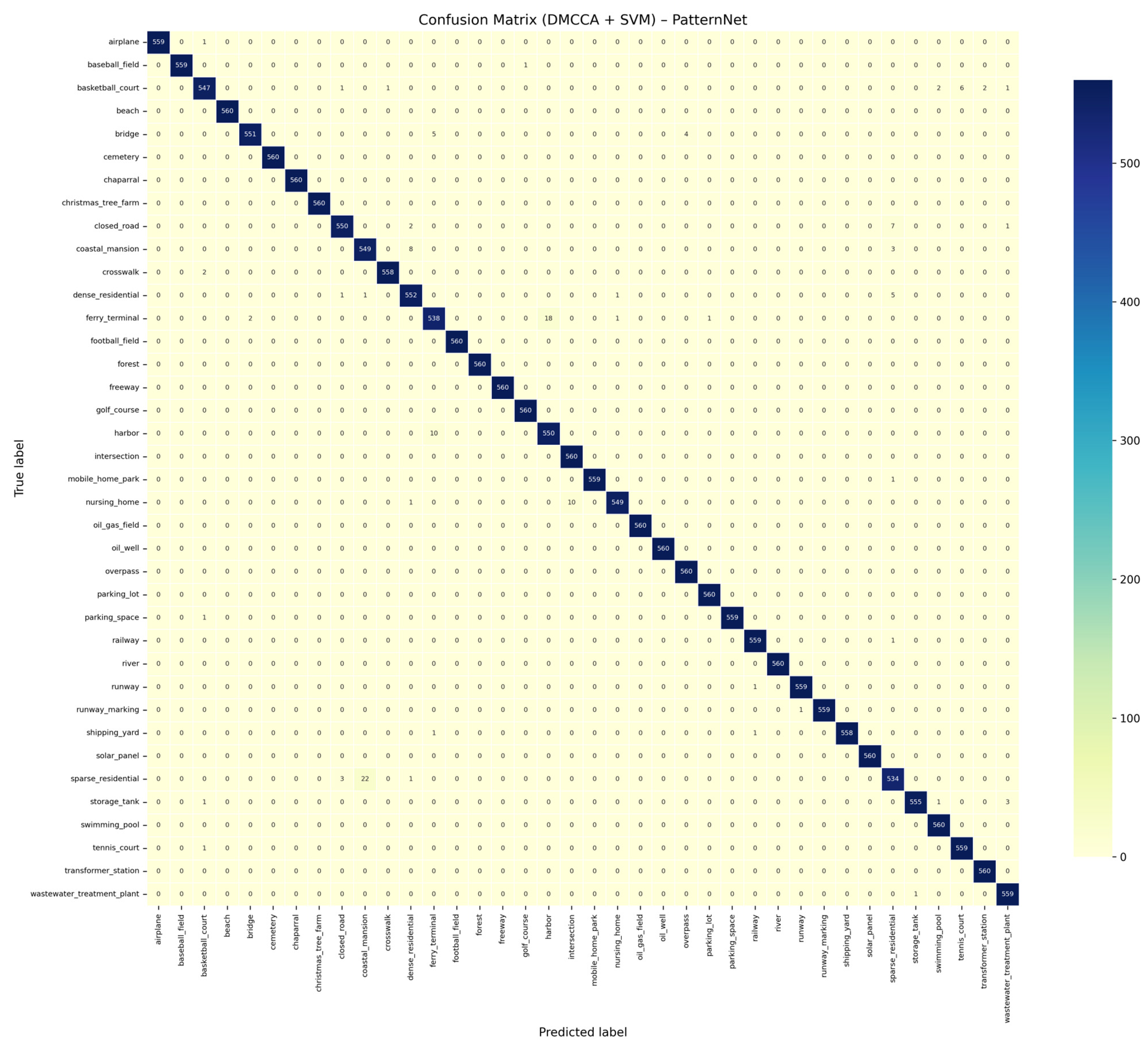
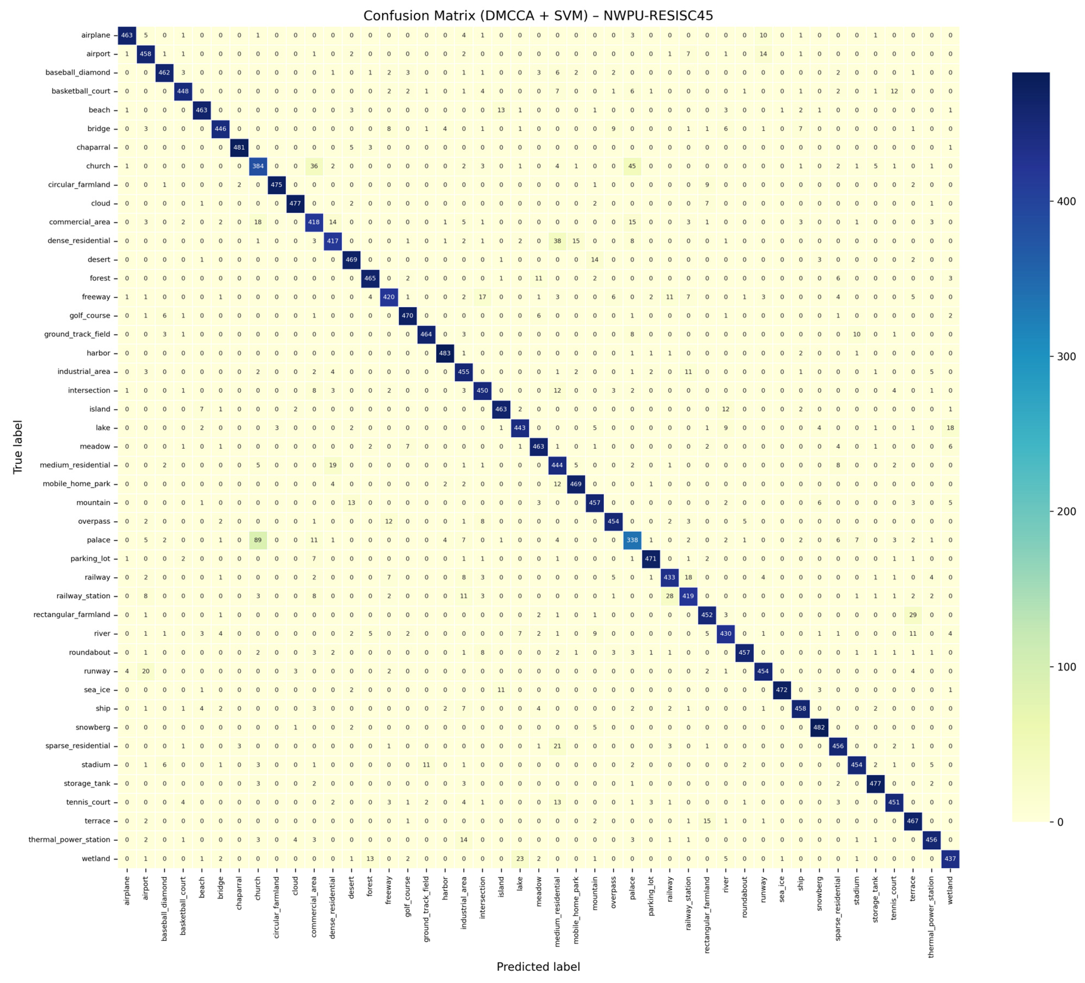
With a 20% training set, the proposed DMCCA + SVM achieved an accuracy of 93.89% on the AID dataset, outperforming the best individual CNN model (DenseNet121, 92.97%) by 0.9%. When the training set was increased to 25%, DMCCA + SVM reached 93.92% accuracy, yielding a larger improvement of 1.35% over DenseNet121 (92.57%). These results indicate that the proposed fusion framework consistently benefits from increased training data while maintaining its relative advantage. On the PatternNet dataset, individual CNN models already achieved very high accuracies (approximately 99%), and therefore only marginal improvements were observed using DMCCA + SVM, ranging from 0.03% to 0.08%. Increasing the training ratio from 20% to 25% resulted in negligible changes in overall performance metrics, suggesting that the dataset is less sensitive to training size due to its balanced structure and visual distinctiveness. Across all datasets, the observed variances remained relatively low, typically within the range of 0.5–0.8%, and were particularly small for the PatternNet dataset. This behavior indicates that the features fused through DMCCA possess strong discriminative capability even under limited training conditions. From a data-efficiency perspective, these results confirm that the proposed approach can achieve robust performance with comparatively small training sets. Moreover, the consistent improvements observed in Precision, Recall, and F1-score further demonstrate that the performance gains are uniform across classes rather than being driven by a subset of categories. 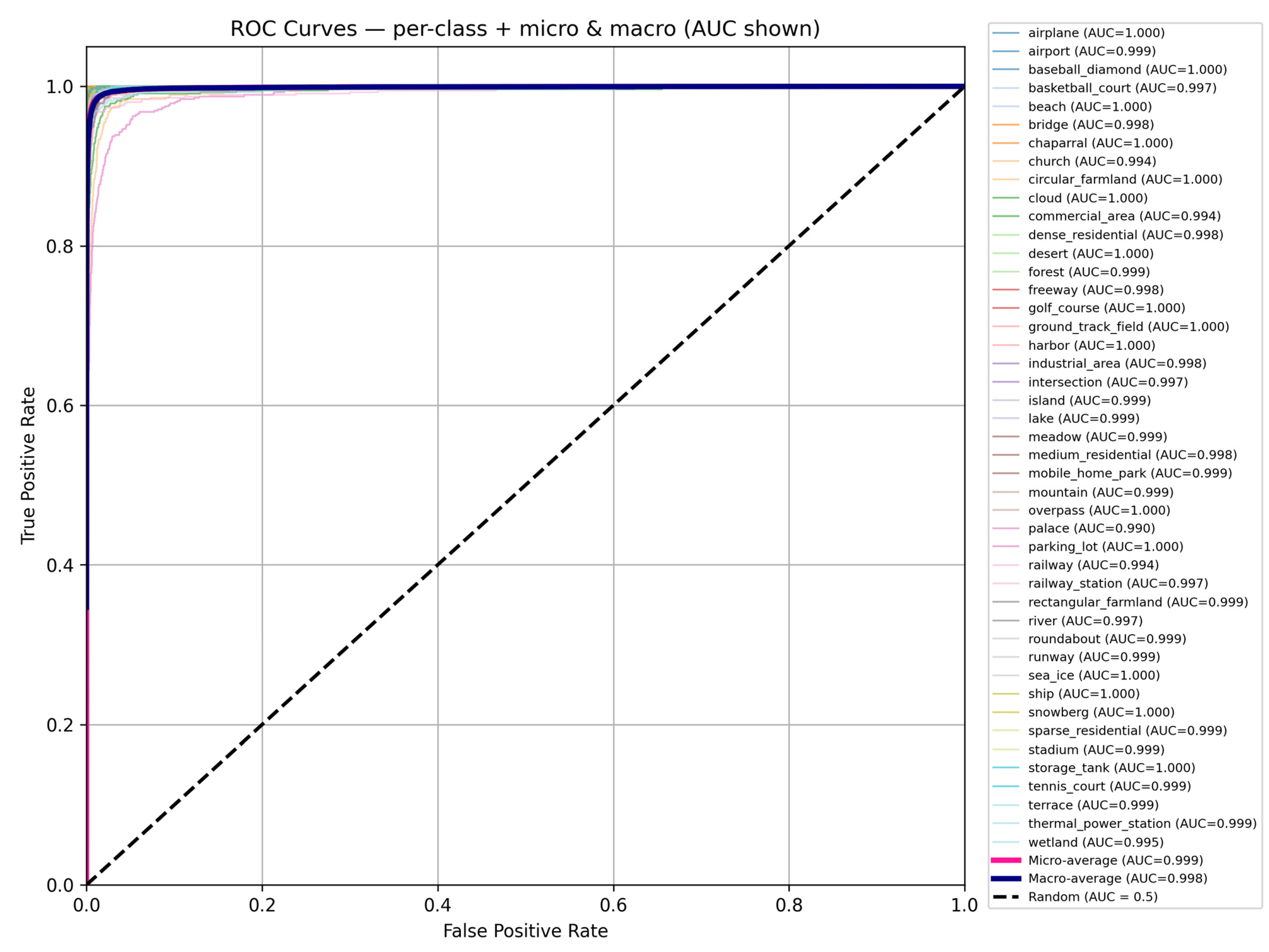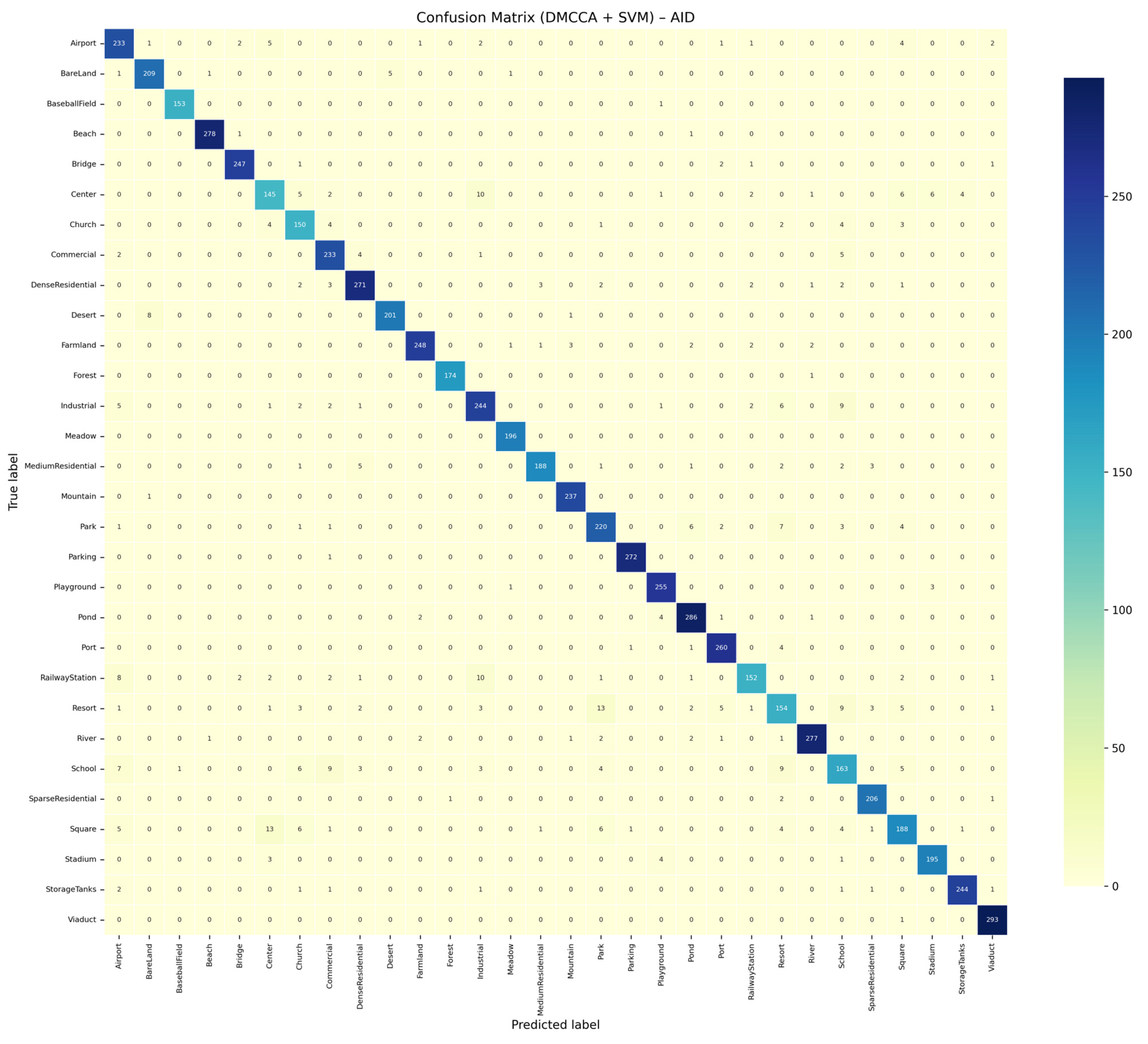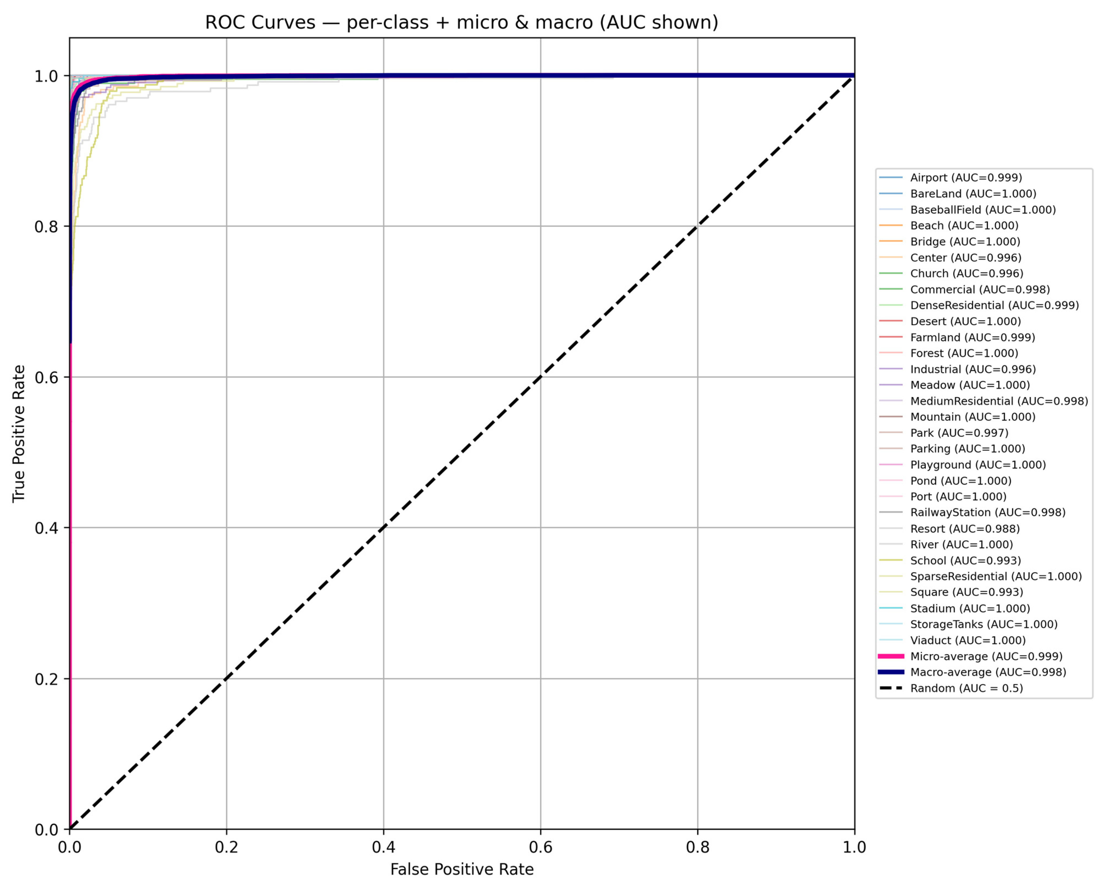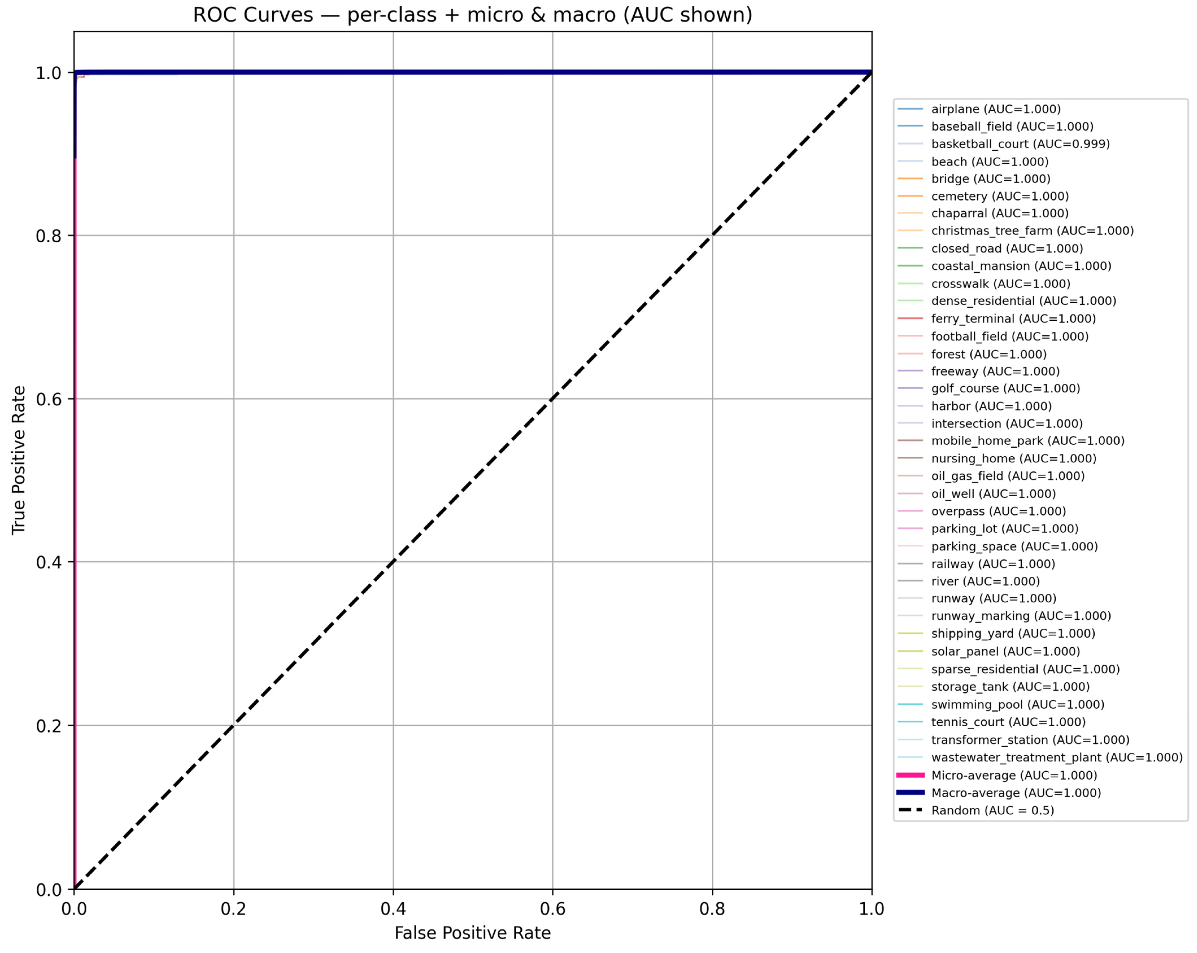The effectiveness of the DMCCA + SVM framework is further supported by the confusion matrices and ROC analyses presented in Figure 2, Figure 3, Figure 4, Figure 5, Figure 6 and Figure 7 for the NWPU-RESISC45, AID, and PatternNet datasets. For the NWPU-RESISC45 dataset, there are 45 scene classes, which are labeled from numbers 0 to 44. The confusion matrix for the DMCCA and SVM model, trained on the 20% training split, shows that 35 out of 45 classes achieved greater than 90% accuracy. “Harbor”, “Snowberg” and “Chaparral”, “Cloud”, and “Storage tank” were the most accurately predicted classes.

The “Palace”, “Church”, and “Commercial area” classes were the most confused. The main reason for this confusion is that the scenes look similar to each other. The “Palace” and “Church” classes are similar in that they have big buildings, domes, and open spaces. The “Commercial area” class visually resembles “Dense residential” and “Industrial area” in terms of texture and building density. Consequently, the model confused these classes due to structural similarities in urban environments.

On the NWPU-RESISC45 dataset, the DMCCA + SVM model demonstrated nearly perfect ROC-AUC results across almost all classes (Figure 3). For most classes, AUC = 1.000 (e.g., Airplane, Beach, Forest, Runway, Harbor, etc.), indicating that the model classified them without errors. In some classes with similar textures, such as Palace, Church, and Commercial_area, the AUC ranged from approximately 0.994 to 0.996, reflecting their visual similarity. Overall, the micro-average AUC = 0.999 and macro-average AUC = 0.998, confirming that the model operates with high sensitivity and a low error rate. These results show that the DMCCA + SVM model is stable and accurate for classifying scenes.

There are 30 scene classes in the AID dataset, and the class labels are integers from 0 to 29. The confusion matrix for the DMCCA + SVM model trained on the 20% training split shows that 22 of the 30 classes got more than 90% correct. The classes of Meadow, Viaduct, Parking, Mountain, Baseball Field, and Forest yielded the most accurate results. The classes that caused the most confusion were the Resort, School, Center, and Square classes. The main reason for this confusion is that these classes look a lot alike. For example, both Resort and Park have green spaces and buildings, while School and Center have areas with a lot of people and buildings and roads, which made the model confused. Also, the fact that there were not many samples in these classes made it hard to train the model, which made it less able to tell them apart.

The DMCCA + SVM model got high ROC-AUC scores for all classes on the AID dataset (Figure 5). For most classes, the AUC is about 1.000 (for example, Beach, Forest, Park, Stadium, Port, Mountain, Viaduct), which means that the model correctly classified them. The AUC for some scenes that looked similar, like Center, Church, Industrial, Resort, and School, was between 0.988 and 0.996, which shows how similar they were. The micro-average AUC is 0.999 and the macro-average AUC is 0.998, which shows that the model works with high sensitivity and low error probability. Therefore, DMCCA + SVM demonstrated stable and accurate classification on the AID dataset.

The PatternNet dataset is a balanced benchmark comprising 38 scene classes, with class labels ranging from 0 to 37. The confusion matrix obtained for the DMCCA + SVM model trained using the 20% training split indicates that all classes achieved classification accuracies exceeding 95%. Minor confusion was observed for the Sparse residential and Ferry terminal classes, which can be attributed to their visual similarity with structurally related categories such as Dense residential and Harbor.

The ROC analysis for the PatternNet dataset (Figure 7) shows consistently high AUC values across all classes. For most classes, the AUC values are very close to 1.0, reflecting strong separability between class boundaries. This behavior can be largely explained by the balanced nature of the dataset and the high inter-class visual distinctiveness present in PatternNet. Together with the confusion matrix results, these findings indicate that the proposed DMCCA + SVM model provides stable and highly discriminative performance on this dataset, without evidence of class-specific instability.

Second Stage. The trained models were evaluated for stability using the K-fold and Random Split methods.

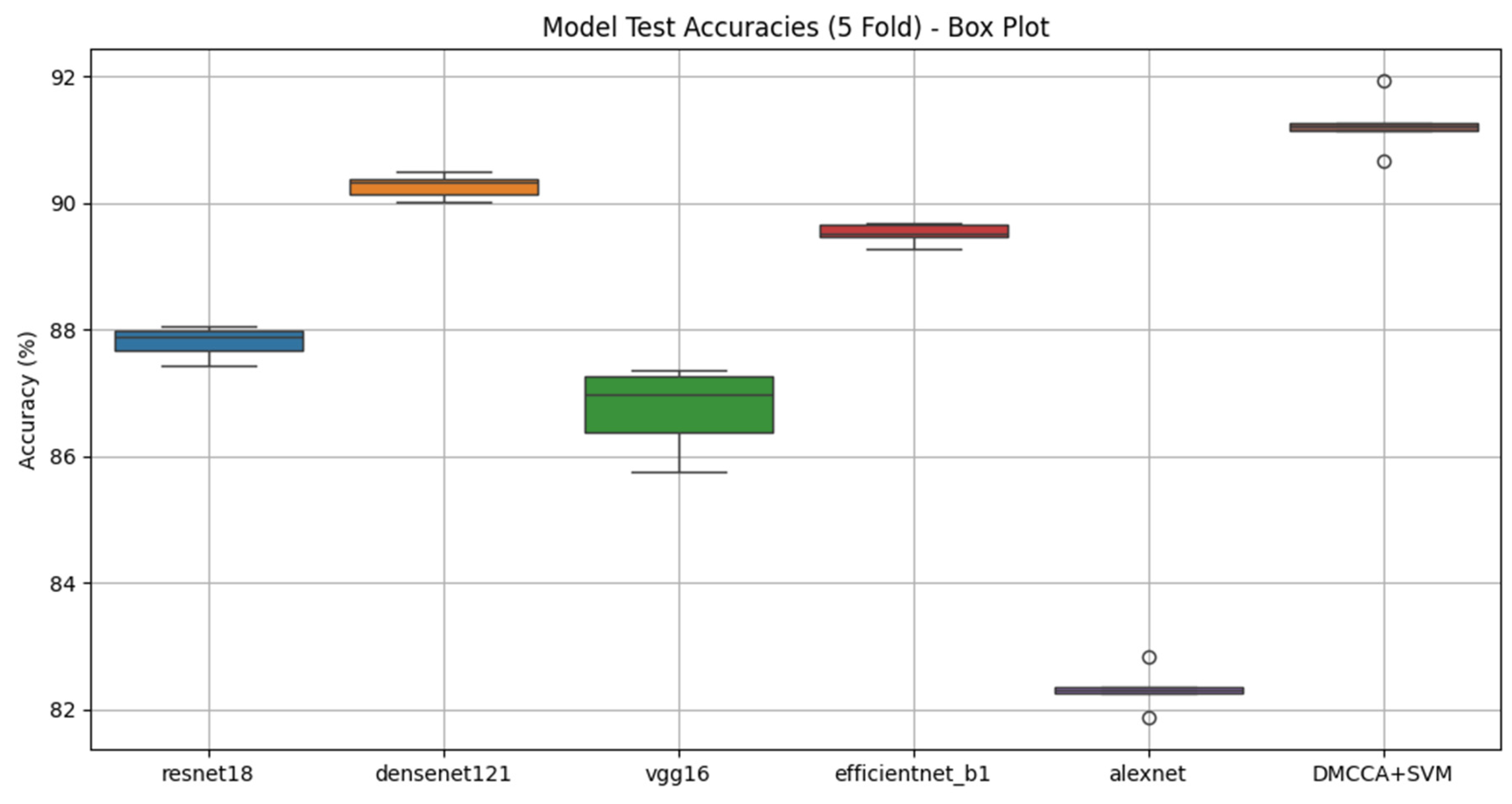
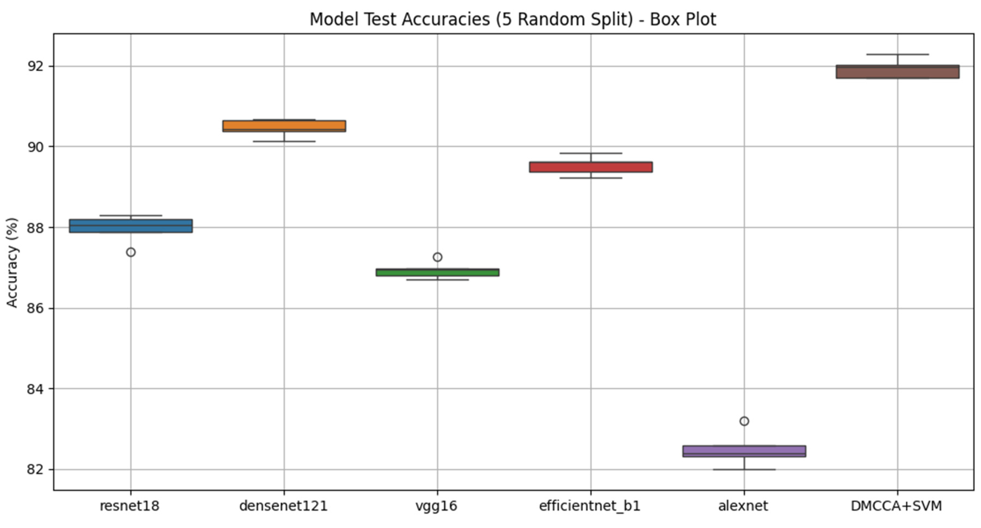
Results for the NWPU-RESISC45 dataset: The experiments conducted on the NWPU-RESISC45 dataset aimed to assess both the accuracy and stability of the models. In this study, multiple deep learning architectures (ResNet18, DenseNet121, VGG16, EfficientNet-B1, and AlexNet) were tested using 5-fold cross-validation and 5 random splits. For each fold and split, all CNN models and the DMCCA + SVM model were evaluated on the same images, ensuring a fairer and more consistent comparison. The test accuracies, standard deviations, and the minimum and maximum accuracy values of each model are provided in

Table 3. Test accuracies on the NWPU-RESISC45 dataset based on 5-fold cross-validation.

Model	Average (%)	Std (σ)	95% CI	Min (%)	Max (%)
ResNet18	87.81	±0.23	[87.61, 88.01]	87.44	88.06
DenseNet121	90.28	±0.17	[90.13, 90.43]	90.02	90.51
VGG16	86.75	±0.60	[86.22, 87.28]	85.75	87.37
EfficientNet-B1	89.52	±0.15	[89.39, 89.65]	89.27	89.69
AlexNet	82.32	±0.31	[82.05, 82.59]	81.87	82.83
DMCCA + SVM	91.25	±0.41	[90.89, 91.61]	90.67	91.94

and

Table 4. Test accuracies on the NWPU-RESISC45 dataset based on 5 random train/test splits.

Model	Average (%)	Std (σ)	95% CI	Min (%)	Max (%)
ResNet18	87.96	±0.32	[87.68, 88.24]	87.38	88.29
DenseNet121	90.45	±0.19	[90.28, 90.62]	90.14	90.67
VGG16	86.94	±0.19	[86.77, 87.11]	86.70	87.27
EfficientNet-B1	89.54	±0.22	[89.35, 89.73]	89.23	89.85
AlexNet	82.50	±0.40	[82.15, 82.85]	82.00	83.20
DMCCA + SVM	91.93	±0.22	[91.74, 92.12]	91.69	92.29

, respectively, to assess the accuracy and reliability of the proposed model and models.

The findings suggest that DenseNet121 exhibited the highest and most stable performance among the individual models, with an average accuracy of 90.28% and a standard deviation of ±0.18 in 5-fold cross-validation. The DMCCA method, which merged features from several models and employed an SVM for final classification, performed better than any individual model, with accuracies of 91.25% in 5-fold tests and 92.13% in random tests. Furthermore, the low standard deviation (±0.23) measured in random tests attests to the robustness of the DMCCA method, which indicates that combining information from separate models improves classification generalizability. Low standard deviations (particularly for DenseNet121 and DMCCA + SVM) suggest that performance is stable across varied splits of the data. Figure 8 and Figure 9 show BoxPlot graphs that visually show these results.

The graphs show that in the box plots of test accuracies for each model, the DMCCA + SVM model achieved the highest performance and maintained a favorable range of accuracy variation. This further illustrates the proposed model’s superiority over individual CNN models.

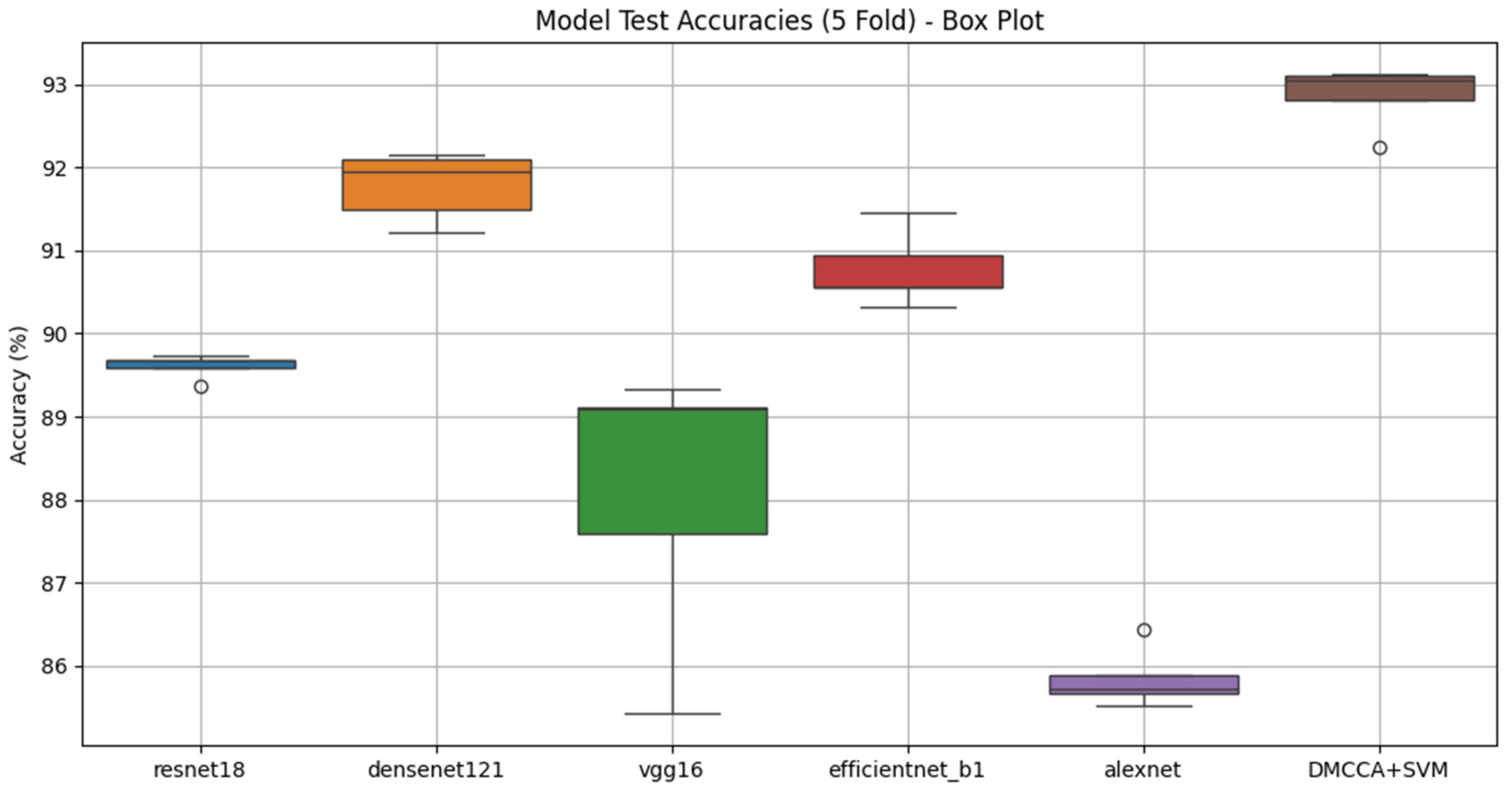
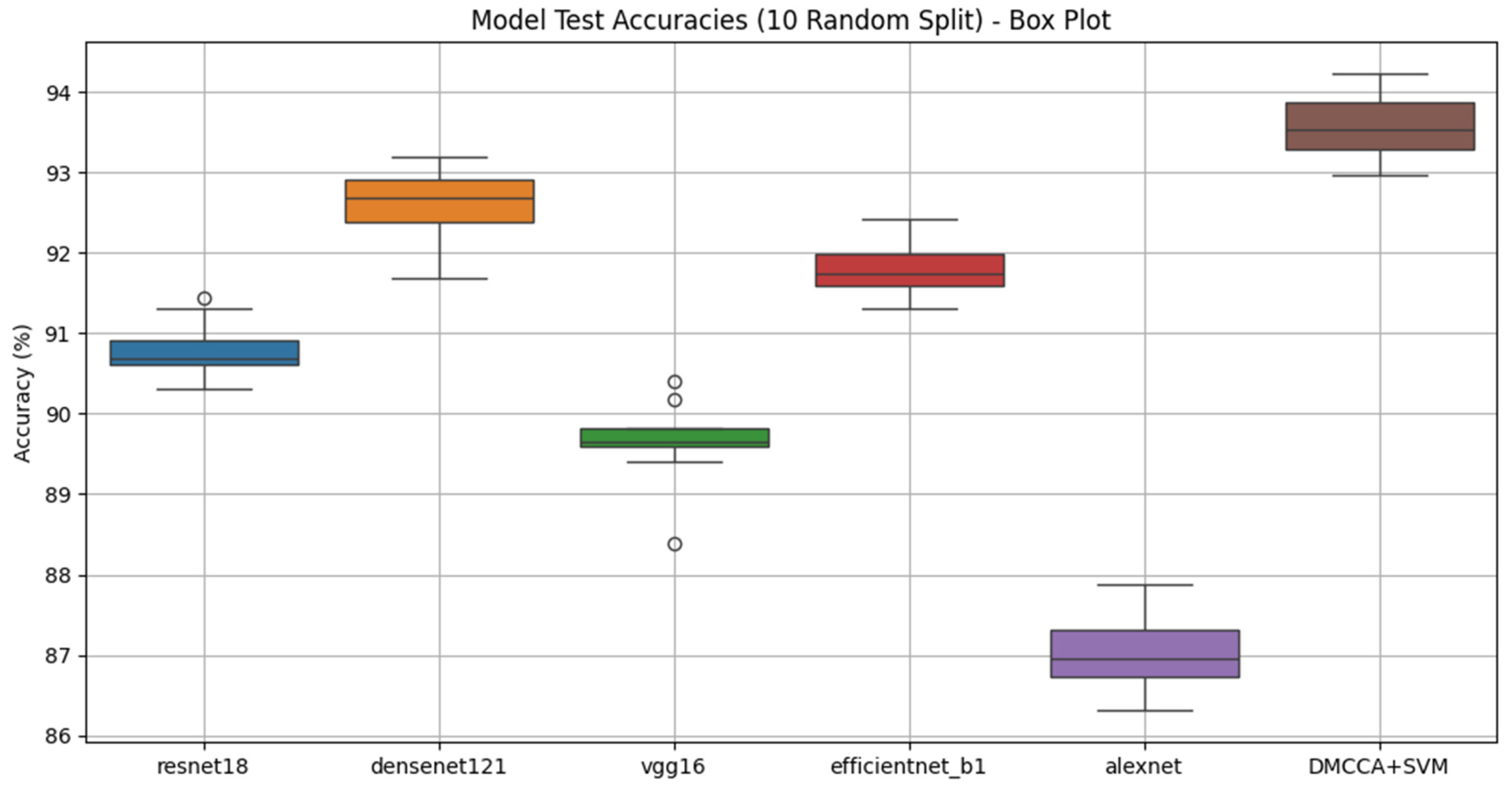
Results for the AID dataset: The experimental analyses conducted on the AID dataset aimed to evaluate the effectiveness of deep learning-based models and the DMCCA-integrated model. In the tests, each of the ResNet18, DenseNet121, VGG16, EfficientNet-B1, and AlexNet models was trained and evaluated separately using 5-fold cross-validation as well as 10 random splits. For this dataset, in each fold and split, all CNN models and the DMCCA + SVM model were tested on the same set of images.

To assess the accuracy and stability of the proposed model and the CNN models,

Table 5. Test accuracies on the AID dataset based on 5-fold cross-validation.

Model	Average (%)	Std (σ)	95% CI	Min (%)	Max (%)
ResNet18	89.61	±0.13	[89.50, 89.72]	89.38	89.74
DenseNet121	91.79	±0.36	[91.47, 92.11]	91.22	92.16
VGG16	88.11	±1.48	[86.81, 89.41]	85.42	87.59
EfficientNet-B1	90.77	±0.40	[90.42, 91.12]	90.33	91.46
AlexNet	85.84	±0.31	[85.57, 86.11]	85.52	86.42
DMCCA + SVM	92.87	±0.33	[92.58, 93.16]	92.24	93.12

and

Table 6. Test accuracies on the AID dataset based on 10 random train/test splits.

Model	Average (%)	Std (σ)	95% CI	Min (%)	Max (%)
ResNet18	90.79	±0.35	[90.57, 91.01]	90.30	91.44
DenseNet121	92.62	±0.45	[92.34, 92.90]	91.69	93.19
VGG16	89.66	±0.53	[89.33, 89.99]	88.39	90.40
EfficientNet-B1	91.78	±0.32	[91.58, 91.98]	91.31	92.41
AlexNet	87.01	±0.49	[86.71, 87.31]	86.31	87.89
DMCCA + SVM	93.58	± 0.44	[93.31, 93.85]	92.96	94.23

report the test accuracy, standard deviation, and minimum—maximum test accuracy for each model.

The DMCCA + SVM model had the highest average accuracy, with 92.87% in cross-validation and 93.58% in random splits, as shown in Table 5 and Table 6. These results show that these models are much better than traditional CNN models. The DMCCA + SVM model surpassed advanced architectures including DenseNet121 (91.79%, 92.62%) and EfficientNet-B1 (90.77%, 91.78%), illustrating its impressive ability to incorporate the features learned from different models. Standard deviation (STD) was used as an indicator of stability during analysis. The DMCCA + SVM model had a STD of ±0.33 related to cross-validation accuracy and ±0.44 related to random splits. This indicates that the method not only achieved high accuracy, but also has a fairly stable classification performance (low dispersion). Figure 10 and Figure 11 show BoxPlot displays of the models and accuracy distributions based on test accuracies from the AID dataset.

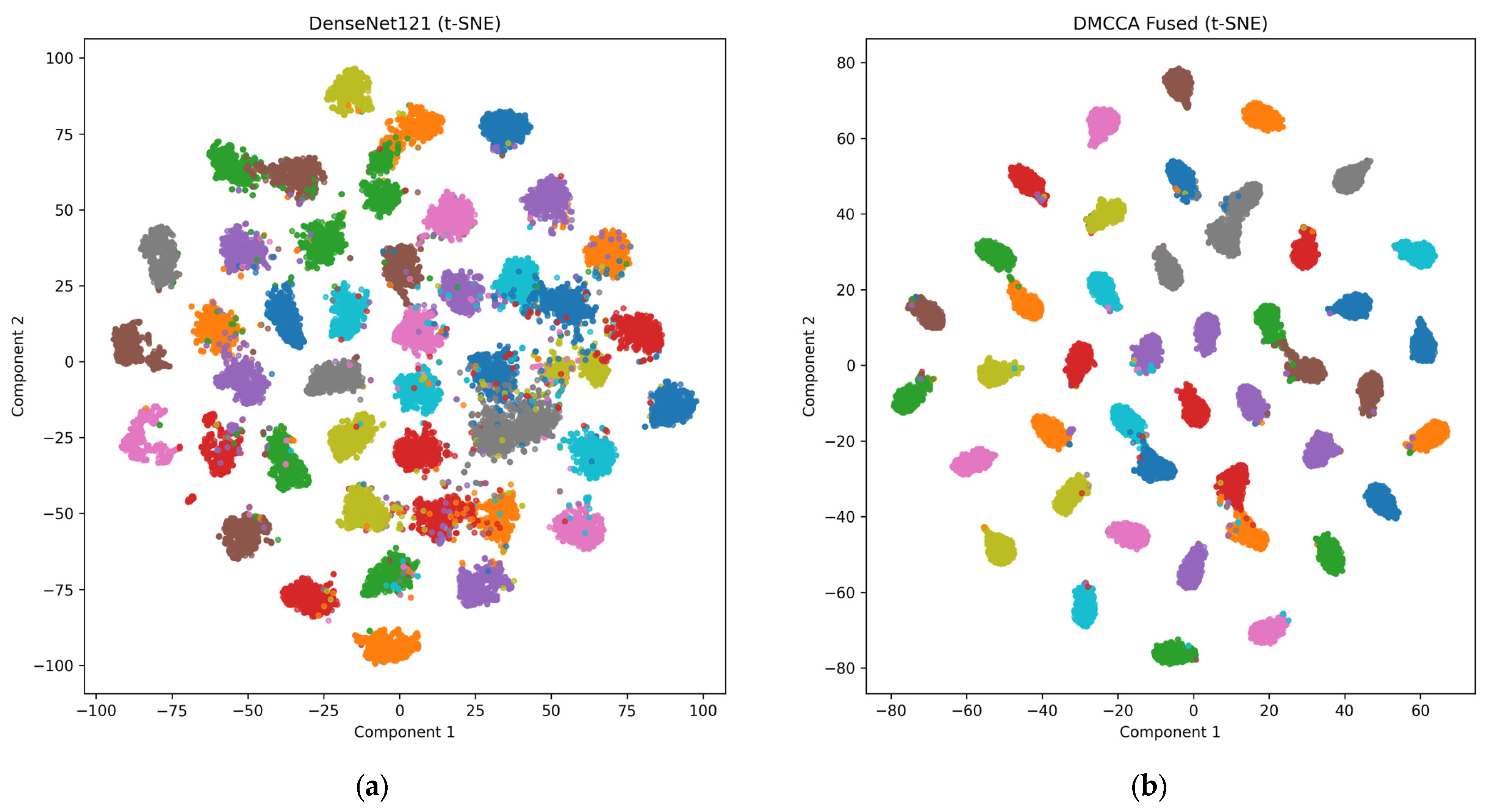
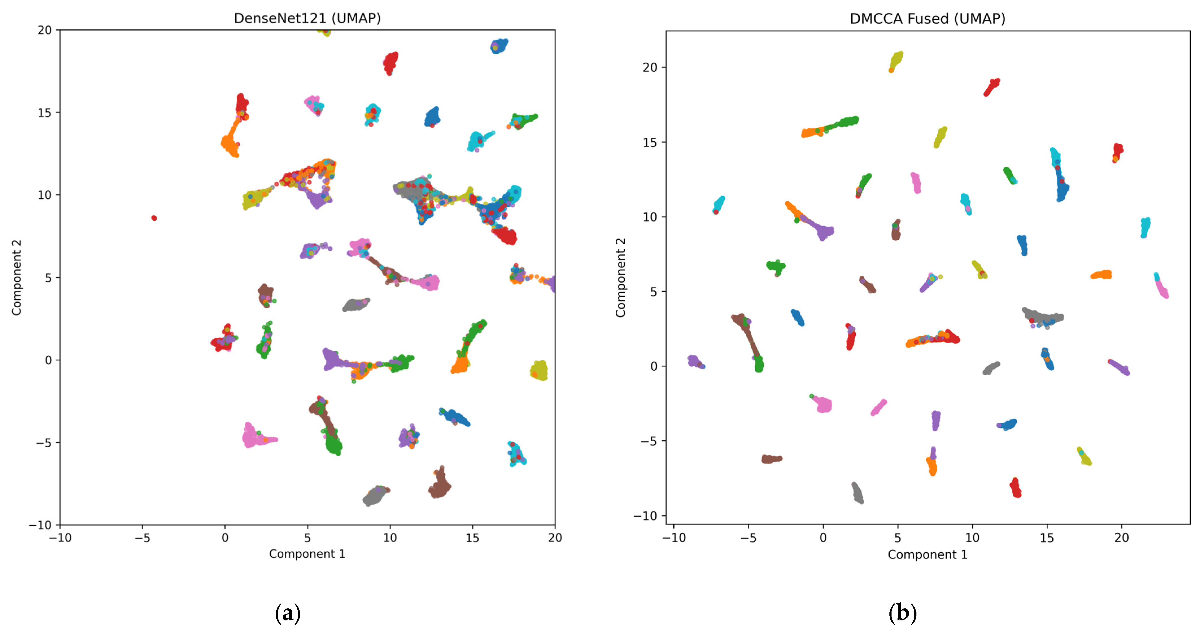
Figure 12 and Figure 13 present a comparative analysis of the t-SNE and UMAP projections of the feature space obtained from the DenseNet121 model, selected as the best-performing individual CNN among the considered architectures, and the feature space fused using the proposed DMCCA approach. While the DenseNet121 model achieves a certain degree of class separability and forms distinct clusters for some classes, noticeable inter-class overlap remains for others. In contrast, the DMCCA-fused feature space exhibits more compact and stable intra-class clusters, resulting in clearer inter-class separation. Both visualization methods demonstrate that the DMCCA approach effectively integrates features extracted from multiple CNN models, significantly enhancing inter-class discrimination. These results confirm that the proposed feature integration strategy produces a more discriminative latent space for classification compared to individual models.

Table 7. Classification performance on the NWPU-RESISC45 dataset (20%/10%/70% train/val/test).

Method	Accuracy (%)	Precision (%)	Recall (%)	F1-Score (%)
ResNet18	88.71	88.84	88.71	88.71
DenseNet121	91.26	91.32	91.26	91.22
VGG16	88.05	88.34	88.05	88.01
Concat + PCA + SVM	14.48	12.78	14.48	12.72
Linear MCCA + SVM	91.80	91.87	91.80	91.78
DMCCA + SVM	92.39	92.50	92.39	92.37

and

Table 8. Classification performance on the AID dataset (20%/10%/70% train/val/test).

Method	Accuracy (%)	Precision (%)	Recall (%)	F1-Score (%)
ResNet18	90.76	90.49	90.36	90.30
DenseNet121	92.77	92.54	92.33	92.32
VGG16	89.63	89.49	89.07	89.05
Concat + PCA + SVM	38.77	36.74	37.29	35.73
Linear MCCA + SVM	92.74	92.39	92.36	92.32
DMCCA + SVM	93.21	93.27	92.71	92.78

present a comparative evaluation of different feature fusion strategies, including Concatenation + PCA + SVM, Linear MCCA + SVM, and the proposed DMCCA + SVM, on the NWPU-RESISC45 and AID datasets using a 20%/10%/70% train/validation/test split. All fusion methods operate on the same CNN-extracted features and are evaluated under identical data partitions.

The results show that Concatenation + PCA + SVM yields substantially lower performance, indicating that simple feature aggregation followed by dimensionality reduction is insufficient for capturing discriminative relationships among heterogeneous deep features. In contrast, Linear MCCA + SVM significantly improves classification performance by modeling inter-feature correlations across multiple views.

The proposed DMCCA + SVM consistently achieves the best results across both datasets, outperforming Linear MCCA in terms of accuracy, precision, recall, and F1-score. This performance gain highlights the importance of incorporating class-discriminative information during feature fusion. Overall, the results confirm that DMCCA provides a more effective and discriminative fusion mechanism than non-discriminative correlation-based and naïve fusion approaches.

In this study, ResNet18, DenseNet121, VGG16, EfficientNet-B1, and AlexNet were initially fine-tuned and evaluated individually. Among them, DenseNet121 achieved the highest standalone accuracy. The selected CNN backbones ensure both strong individual performance and architectural diversity, enabling an effective evaluation of the proposed DMCCA-based feature fusion framework. Importantly, the objective of this work is not limited to fusing only the strongest models, but rather to demonstrate the ability of DMCCA to improve overall performance by integrating CNNs with different performance levels and complementary representations. Accordingly, ResNet18 and VGG16 were included in the fusion, while AlexNet was excluded due to its relatively low effectiveness. Although incorporating EfficientNet-B1 could further enhance performance, a limited yet representative set of models was selected to highlight the generality and robustness of the proposed approach. The integration of a larger number of CNN models is left for future work.

It should be noted that the absolute performance values reported in Table 7 and Table 8 show slight differences compared to those presented earlier in Table 2. These variations arise from different random realizations of the train/validation/test split, while maintaining identical split ratios and consistent data partitions across models within each experimental setting. Such variations are common in deep learning-based evaluations, particularly when limited training data are used. Importantly, despite these differences, the relative performance trends remain consistent, with DMCCA + SVM consistently outperforming alternative fusion strategies and individual CNN baselines.

In addition to mean accuracy and standard deviation, 95% confidence intervals were computed to evaluate statistical reliability. As shown in Table 3, Table 4, Table 5 and Table 6, DMCCA + SVM consistently achieves higher accuracy with narrow confidence intervals and limited overlap with individual CNN models, indicating that the observed gains are statistically meaningful. This conclusion is further supported by low variance values and boxplot visualizations in Figure 10 and Figure 11, which confirm the stability of the proposed method across multiple runs.

Overall, the combination of DMCCA for feature fusion and SVM for classification provides an effective and reliable framework for remote sensing scene classification. The experimental results demonstrate that DMCCA enables the construction of a more discriminative and robust latent feature space compared to single-model and non-discriminative fusion approaches, making it well suited for complex remote sensing scenarios.

7. Conclusions

In the research, remote sensing images were mined for their features and characterized as scenes through several deep convolutional neural networks (CNNs) like ResNet18, DenseNet121, VGG16, EfficientNet-B1, and AlexNet. Their performance was evaluated by different experiments. The tests carried out on complex and high-resolution datasets like NWPU-RESISC45 and AID indicated that individual models, even though their accuracy was relatively high, were very often unstable and not able to generalize. DenseNet121 was the model with the highest accuracy across both datasets, but it had a slightly worse performance during some folds. VGG16 and AlexNet ranked lower than the other models, and this was probably due to their shorter layer designs and smaller numbers of parameters. The opposite was the case for the proposed DMCCA-based feature fusion method, which had both high accuracy and stability. The SVM classifier that was trained on the features extracted using this method averaged surpassing the individual CNN models for both datasets. Furthermore, the DMCCA + SVM results exhibited a small STDEV, which points to the fact that this method is reliable and could be used in different situations. The results imply that interoperability of features from various heterogeneous models adds to the data’s semantic content and as a result, the final classifier is more powerful. Methods for fusing features from diverse sources are extremely important for scene classification systems that handle high-resolution and multi-class images. All in all, the proposed model shows considerable improvements in terms of accuracy, stability, and effectiveness in classifying scenes using remote sensing images.