Spatiotemporal Dynamics of the Liaohe Delta (1987–2017) Using an Integrated Classification and Feature Selection Approach

Abstract

Wetland landscape classification is fundamental to monitoring changes in ecosystem patterns. This study proposes an ensemble classification approach that integrates Maximum Likelihood Classification (MLC) and Decision Tree (DT) methods with optimized feature selection for long-term wetland monitoring in the Liaohe Delta, China. Based on four periods of Landsat remote sensing images from 1987, 1997, 2007, and 2017, multi-dimensional features including PCA1, TCT, NDVI, and MNDWI were extracted to construct a hierarchical classification system comprising 13 landscape types. The results show that the integrated method achieved an overall classification accuracy of 87.71% and a Kappa coefficient of 0.85, improving by 16.50% and 19.72%, respectively, compared with the single MLC approach. The classification results reveal significant spatiotemporal variations in landscape patterns. Reed wetlands decreased from 1284.44 km² in 1987 to 1006.70 km² in 1997, followed by a recovery to 1275.53 km² in 2017. In contrast, Suaeda communities experienced severe degradation, declining sharply from 227.48 km² in 1987 to 30.52 km² in 2017. Meanwhile, the coastline advanced landward by 263.24 km², with the proportion of artificial shoreline increasing from 12.4% to 38.7%. The changes in wetland landscape types in the Liaohe Delta from 1987 to 2017 were mainly influenced by urbanization processes and ecological restoration policies. These findings indicate that the proposed method can effectively support long-term wetland landscape dynamics analysis and provide a useful reference for coastal wetland management.

1. Introduction

1.1. Background and Significance

Wetlands are among the most biologically diverse and functionally critical ecosystems on Earth, providing essential ecosystem services such as flood regulation, water purification, carbon sequestration and oxygen release, and biodiversity conservation [1]. As transitional zones between terrestrial and marine environments, coastal wetlands are subjected to the combined pressures of climate change and human activities, making them hotspots for research on ecologically vulnerable regions worldwide. Accurate characterization of wetland landscape classification and its dynamic changes is therefore of great scientific importance for ecological health monitoring, conservation policy formulation, and sustainable management [2].

Remote sensing technology offers a cost-effective approach for large-scale wetland monitoring. Land use types have been classified through visual interpretations of Landsat images; however, the land cover types (associated with several reclamation activities) representing the 1960s were derived from vectorizations of topographic maps and local land use maps [3,4]. However, coastal wetlands are characterized by diverse land cover types, complex spectral signatures, and strong spatial heterogeneity, making it difficult for a single classification method to achieve high accuracy [5,6,7]. Various approaches, including object-based classification [8], Support Vector Machines (SVM) [9], Classification and Regression Tree (CART)-based iterative classification [10,11], Artificial Neural Networks (ANN) [12], Deep Learning (DL) [13,14,15,16,17,18], and Random Forest algorithms [19,20,21,22,23,24], have been successfully applied in coastal wetland studies, achieving Kappa coefficients ranging from 0.83 to 0.89. As a classical supervised classification method, Maximum Likelihood Classification (MLC) assumes that samples follow a normal distribution and performs probabilistic discrimination for land cover identification [25]. It has advantages in terms of accuracy and stability; however, its ability to distinguish spectrally similar classes is limited in complex wetland environments. In contrast, Decision Tree (DT) methods can integrate multi-source information such as spectral indices and elevation data, offering high computational efficiency and flexibility, but they are less effective in fine-grained, multi-level classification tasks [26].

Previous studies have demonstrated that integrating raw remote sensing data with feature parameters and combining multiple classification methods is an effective strategy for improving classification accuracy in complex and heterogeneous wetlands [27,28,29,30,31,32,33,34]. Nevertheless, most existing studies focus on single classifiers or approaches without feature integration. Applications that combine multi-feature parameters with multi-classifier ensembles for long-term wetland landscape dynamic monitoring remain insufficiently explored.

1.2. Study Area and Related Work

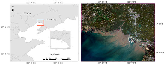
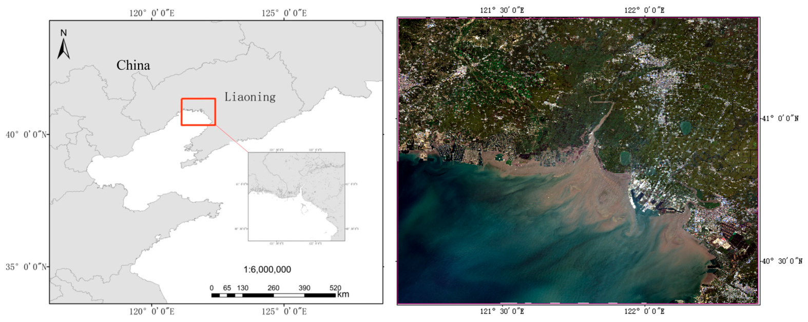
The Liaohe Delta is located in the southwestern part of Liaoning Province, China (121°25′–122°30′ E, 40°40′–41°25′ N). It is one of the most important estuarine wetlands in China and hosts the largest reed wetland distribution in Asia (Figure 1). The major rivers sustaining wetland habitats in this region include the Daling River, Xiaoling River, Shuangtaizi River, Daliao River, and Daqing River. The area is characterized by a warm temperate continental semi-humid monsoon climate, with distinct seasons, fertile soils, and diverse vegetation types. The dominant plant communities are Phragmites australis and Suaeda salsa, forming unique landscapes known as “reed marshes” and the “red beach.” These habitats also provide critical breeding and foraging grounds for rare and endangered bird species, such as Grus japonensis, Ciconia boyciana, and Larus saundersi [19,35].

Figure 1. Mosaicked image of the study area in the Liaohe Delta, Liaoning Province, China.

Over the past three decades, the Liaohe Delta has undergone dramatic landscape changes. Previous studies have applied GIS and remote sensing techniques to investigate these dynamics. For example, Li analyzed the degradation of reed and Suaeda salsa wetlands from 1986 to 2012 based on visual interpretation [36]; Liu and others examined wetland changes from 1982 to 2015 using human–computer interactive interpretation [37]; and Yin extracted five wetland types for the period 2000–2013 using supervised classification methods [38]. However, most of these studies relied on single classifiers or approaches without feature integration, leading to limitations in classification accuracy, category refinement, and long-term dynamic monitoring.

To address these limitations, this study introduces the following improvements: (1) integrating MLC and DT methods with optimized feature selection to construct a three-level landscape classification system comprising 13 categories; (2) achieving long-term information extraction for the period 1987–2017; (3) quantitatively revealing the spatial relationships between coastline changes and wetland type transitions through GIS-based spatial analysis; and (4) explicitly identifying the limitations of the proposed method.

1.3. Objectives

This study aims to: (1) Develop a classification framework integrating MLC and DT methods, optimize feature selection, and compare its performance with mainstream approaches under the same conditions; (2) Construct a three-level landscape classification system comprising 13 categories for the Liaohe Delta, and achieve long-term wetland information extraction for the period 1987–2017; (3) Reveal the spatiotemporal evolution patterns of wetland landscape configurations and analyze the spatial relationships between coastline changes and wetland type transitions; (4) Carefully examine the driving factors of wetland evolution, explicitly identify the limitations of the study, and provide references for future research.

2. Methodology and Data

2.1. Data Sources

The data used in this work were collected from the geospatial data cloud (http://www.gscloud.cn) and included Landsat 8 Operational Land Imager (OLI), Landsat 5 Thermal Mapper (TM) and Advanced Spaceborne Thermal Emission and Reflection Radiometer (ASTER) Global Digital Elevation Model Version 2 (GDEMV2) data, as shown in Table 1. Image selection criteria include: (1) Cloud cover less than 10%; (2) Acquisition during September to October to minimize phenological differences and tidal effects; (3) Temporal interval of approximately 10 years; (4) Landsat series data were selected due to their 30 m spatial resolution, 16-day revisit cycle, and long-term continuous archive. Data from different sensors were harmonized using relative radiometric normalization to ensure consistency.

Table 1. Remote sensing image information of the study area.

Imaging Carrier	Sensor	Imaging Time	Number of Scenes	Spatial Resolution (m)	Cloud Cover (%)	Rationale for Data Selection
Landsat 5	TM	21 September 1987	2	30	<5	Reference year with no cloud cover
Landsat 5	TM	18 October 1997	2	30	<8	Period of intensive agricultural development
Landsat 5	TM	28 September 2007	2	30	<3	Period of policy adjustment
Landsat 8	OLI	7 September 2017	2	30	<5	Recent land-use conditions
ASTER	ASTER	2015	4	30	-	Elevation reference data

The specific data sources used in this study include six Landsat 5 TM images, two Landsat 8 OLI images, and four ASTER GDEM V2 datasets, all with a spatial resolution of 30 m. The satellite images were taken from September to October, were basically free of cloud cover in the study area and were of good quality. Therefore, 2 scenes from 21 September 1987, 2 scenes from 18 October 1997, 2 scenes from 28 September 2007, and 2 scenes from 7 September 2017 were used in the research. The ASTER GDEM V2 global Digital Elevation Model (DEM) data were officially released on 6 January 2015, and we used this data source in the information extraction and classification processes as one of the parameters of the decision tree. This DEM of Earth’s land surface contains 1.3 million stereo images collected by Japan’s ASTER satellite. Its horizontal accuracy reaches 30 m. ASTER’s accurate terrain data can be used in the fields of natural resource inclusion, environmental management, geology and urban planning.

2.2. Technical Workflow and Feature Parameter Fusion Strategy

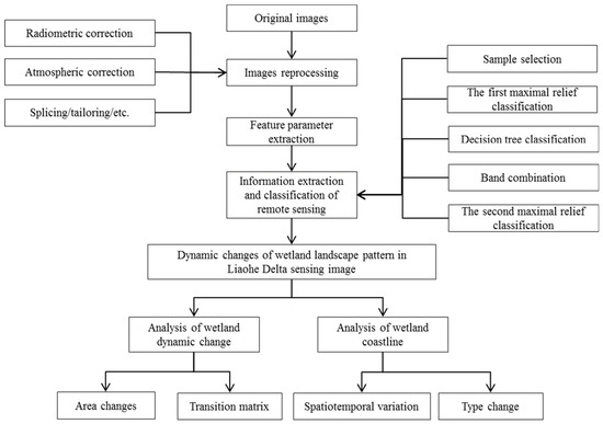
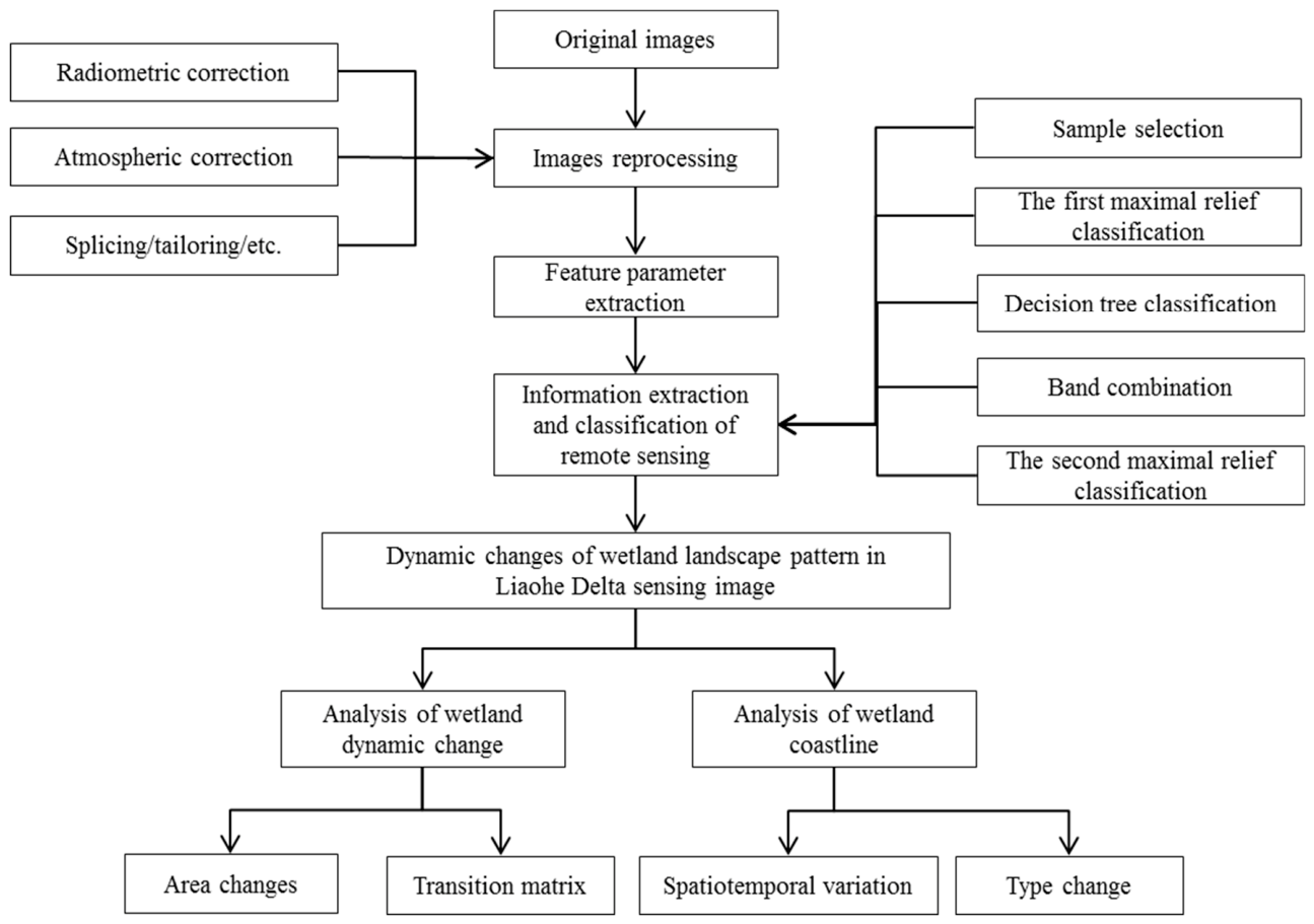
A radiometric correction, an atmospheric correction, and splicing and cropping steps were performed on the downloaded remote sensing images and DEM data representing 2017, 2007, 1997, and 1987; in addition, we applied a ground reflectivity extraction on the cropped remote sensing data and a feature extraction. The characteristic parameter bands were combined, and the specific technical route describing the methodology is shown in Figure 2.

Figure 2. Technical route used in this study.

(1) Image preprocessing

The preprocessing of the remote sensing imagery used in this study mainly included sensor radiometric correction, atmospheric correction, image mosaicking, and clipping. Radiometric correction refers to the conversion of original DN value into a value indicating the reflectivity of the outer surface of the atmosphere, with the aim of eliminating errors generated by the sensor itself. Atmospheric correction further converts radiance or apparent reflectance into true surface reflectance, thereby removing the effects of atmospheric scattering, absorption, and reflection. For the study area, all available cloud-free Level-1 terrain-corrected images were acquired, with data projected in the Universal Transverse Mercator (UTM) coordinate system and based on the World Geodetic System 1984 (WGS84). In addition, considering the specific objectives of this study and the geolocation accuracy of Landsat OLI and TM data products (with circular errors of less than 12 m), no further geometric correction of the Landsat imagery was required [39].

(2) Feature parameter extraction

Nine feature parameters were derived based on surface reflectance data. Among them, PCA1, TCT Brightness, NDVI, MNDWI, RED, and Near-Infrared Band (NIR) are spectral features; Soil Index (SI) and urban building index (Index-based Build-up Index, or IBI) are index-based features; and DEM is a topographic feature. The feature fusion strategy involved combining the original multispectral bands (six bands) with the extracted feature parameters (nine variables) (Table 2), forming a 15-dimensional feature space to enhance the separability of land cover types.

Table 2. Statistics of characteristic parameters.

ID	Name	Comments on a Form	Classification Function
1	PCA1	The first component of principal component analysis (PCA) of original remote sensing data [40,41,42,43]	Dimensionality reduction and noise removal
2	TCT Brightness	The brightness component of tassel HAT transform (TCT) of original remote sensing data	Distinguishing brightness differences
3	NDVI	Normalized Difference Vegetation Index	Enhancing vegetation information
4	MNDWI	Modified Normalized Difference Water Index	Accurate extraction of water bodies
5	RED	Red band spectral value of original remote sensing data (can enhance the contrast between vegetation coverage and non-vegetation coverage)	Enhancing vegetation contrast
6	NIR	The near-infrared spectral values of the original remote sensing data (the most sensitive to the difference in green plant types, clear water contour, used to enhance the contrast between soil crop and land water)	Discriminating green vegetation
7	SI	Bare Soil Index [36]	Identifying bare land surfaces
8	IBI	Index-based Build-up Index [41,44]	Extraction of impervious surfaces
9	DEM	The land surface elevation data of the ASTER sensor can be downloaded directly from the spatial geographic data cloud website	Terrain differentiation support

PCA is widely used in related research on vegetation coverage [40], in the remote sensing monitoring of ecological changes [41,42], and in ground feature classifications [29,43]. PC variables can be repeated (to indicate relationships) for all the originally proposed variables. Similar variables indicate redundancy, and PCA can establish as few new variables as possible and ensure that these new variables are pairwise-unrelated, allowing them to retain the original information to the greatest possible extent when reflecting information on the subject.

The TCT, also known as the KT transformation or Kauth–Thomas transformation, is an empirical linear orthogonal transformation of images based on the information distribution structure of soil and vegetation; this transformation is applied in multispectral remote sensing research performed in a multidimensional spectral space. After the transformation, the first three components are named “brightness”, “greenness” and “moisture”; these components reflect the soil rock, vegetation, and moisture information in soil and vegetation, respectively. The PCA data were converted using the Tasseled Cap module in ENVI software (Version 5.3).

The NDVI is one of the most commonly used indexes for indicating the growth status of vegetation. It is widely used in the fields of vegetation growth and ecological environmental quality monitoring. The improved normalized difference water index (MNDWI, or modified NDWI) was used to extract water body information from images. The MNDWI can effectively distinguish shadows and water bodies and solves the difficult problem of removing shadows during the water body extraction process.

Bare soil is the main surface landscape in the soil erosion area. This datum thus plays an extremely important role in the monitoring and management of soil erosion. The calculation formula of the Bare Soil Index (SI) is based on Zhou [19].

The calculation formula of the urban building index IBI is shown in Formula (1) [39,40,41]:

$$\mathrm{I}\mathrm{B}\mathrm{I}={\displaystyle \frac{2\rho \left(swir2\right)/(\rho \left(swir1\right)+\rho (nir\left)\right)-[\rho \left(nir\right)/(\rho \left(red\right)+\rho \left(nir\right))+\rho \left(green\right)/(\rho \left(swir1\right)+\rho \left(green\right)\left)\right]}{2\rho \left(swir2\right)/(\rho \left(swir1\right)+\rho (nir\left)\right)-[\rho \left(nir\right)/(\rho \left(red\right)+\rho \left(nir\right))+\rho \left(green\right)/(\rho \left(swir1\right)+\rho \left(green\right)\left)\right]}}$$

(1)

In Formula (1), $\rho \left(nir\right)$ represents the surface reflectance value of the near-infrared wave band, $\rho \left(green\right)$ represents the surface reflectance value of the green wave band, $\rho \left(red\right)$ represents the red-band surface reflectance value, $\rho \left(swir1\right)$ represents the surface reflectance value of the shortwave infrared 1 band, and $\rho \left(swir2\right)$ represents the surface reflectance value of the shortwave infrared 2-band.

(3) Ensemble classification

The ensemble classification consists of three steps: MLC, DT classification, and band stacking with secondary classification.

Step 1: MLC (input: six multispectral bands). MLC was applied to perform baseline land cover classification based on probabilistic decision rules.

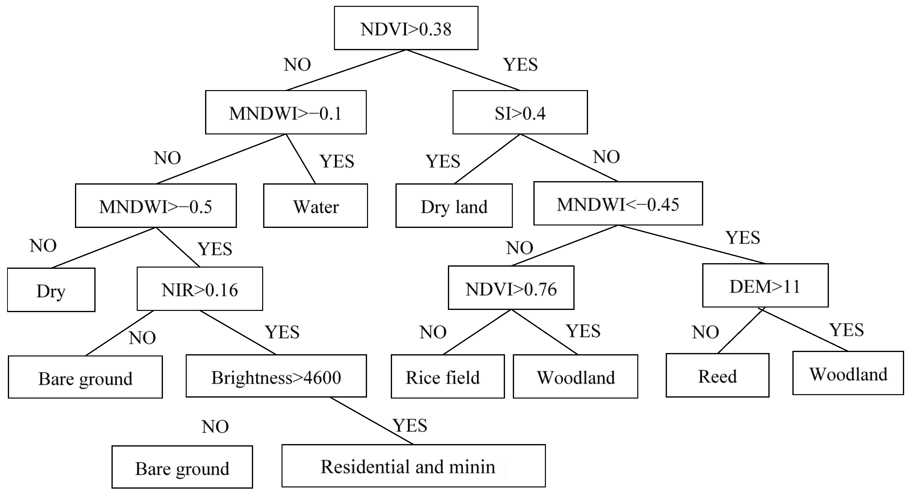
Step 2: DT classification (input: six selected feature parameters, i.e., Brightness, NDVI, MNDWI, NIR, SI, and DEM). The decision thresholds were determined based on critical breakpoints identified from spectral histogram distributions, providing auxiliary classification information.

Step 3: Band stacking and secondary classification. The MLC result (one band), the DT classification result (one band), and nine feature parameters (nine bands) were combined using the ENVI LayerStack module to generate an 11-band dataset. A second-round MLC was then performed on the fused dataset. The fusion principle is based on the complementarity of the three components: the MLC result provides a probabilistic spectral foundation, the DT result offers rule-based auxiliary constraints, and the feature parameters enhance inter-class separability. Together, these components work synergistically to improve overall classification accuracy.

2.3. Quantitative Contribution Analysis of Each Component and Comparative Experimental Design

Regarding the remote sensing image of Liaohe Delta in 2007, by comparing the single DT classification results with the single MLC results and the MLC effect of the combined method, we found that the classification results obtained with the combined method were the most accurate. To clarify the contributions of each component and the positioning of the proposed method, a set of comparative experiments was designed.

Supervised classification using MLC was first conducted by selecting appropriate training samples to automatically extract land cover information. The main advantages of MLC include high classification accuracy and low random error. However, in practice, classification based on a single data source still exhibited certain misclassification issues. Field validation points indicated that the overall classification accuracy reached 75.29%, with a Kappa coefficient of 0.71, and reed vegetation was incorrectly identified in upland dry land areas.

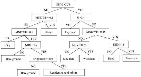
DT classification, which integrates multiple input variables for automatic classification, offers advantages in computational efficiency and flexibility. In this study, six feature parameters—Brightness, NDVI, MNDWI, NIR, SI, and DEM—were selected based on previous studies [8,9,10,11,25,26,29]. The DT-based classification was performed for preliminary wetland mapping. The parameter thresholds were determined according to the critical breakpoints in spectral histogram distributions of different land cover types. However, the DT approach still suffered from confusion among forestland and dry farmland, rice paddies and reed wetlands, as well as bare land and residential areas (Figure 3). Moreover, it failed to achieve the full 13-class classification scheme; for example, water bodies were identified but not further subdivided into rivers, reservoirs, and shallow water zones. As a result, its classification performance was relatively low, with an overall accuracy of 56.82% and a Kappa coefficient of 0.57. Therefore, the DT classification method is not suitable for fine-scale (three-level) landscape classification in complex wetland environments.

Figure 3. Parameter setting of decision tree.

Finally, the classification results obtained from the DT method, the initial MLC results, and nine additional feature parameters were combined through band stacking for a second-stage information extraction. The results showed a significant improvement, with an overall classification accuracy of 87.71% and a Kappa coefficient of 0.85 (Table 3), demonstrating the effectiveness and suitability of the proposed interpretation framework.

Table 3. Results of comparative experiments.

Experimental Scheme	Input Data	Overall Accuracy (%)	Kappa Coefficient	Improvement over Baseline (%)
Original bands (MLC)	6 multispectral bands	75.29	0.71	baseline
Feature parameters (MLC)	9 feature parameters	80.15	0.77	+4.86
Original bands (DT)	6 multispectral bands	52.38	0.52	No improvement
Feature parameters (DT)	6 selected features	56.82	0.57	+4.44
Simple combination (MLC & DT)	MLC result & DT result	79.63	0.76	+4.34
Integrated (MLC & DT)	MLC result & DT result & 9 feature parameters	87.71	0.85	+12.42

It should be noted that the above comparisons were conducted only within the MLC–DT framework and did not include currently advanced mainstream methods such as object-based SVM or Random Forest. The accuracy achieved in this study (Kappa = 0.85) is comparable to that reported in previous studies using object-based SVM (Kappa = 0.84~0.89) [26] and Random Forest (Kappa = 0.83~0.87) [29]. With respect to the comparison with advanced classifiers such as Random Forest and Support Vector Machine, we acknowledge that the current comparison is literature-based rather than derived from same-dataset benchmarking experiments. However, since these methods were not evaluated under identical conditions (i.e., the same study area and validation dataset), it is not appropriate to conclude that the proposed method outperforms these advanced approaches. Future research should incorporate such comparative experiments to further validate the advantages of the proposed method.

2.4. Classification System and Category Aggregation Description

Wetland classification is the basis of wetland research. The classification schemes of wetland ecosystems differ according to the purpose of the study, the characteristics of the study area, and the local land use/cover characteristics. The Liaohe Delta region contains diverse landforms, including large areas of natural wetlands such as reeds and beaches and large areas of rice fields and dry lands. At the same time, as a coastal area, the development of the coastal zone has formed a large artificial wetland area.

Based on the characteristics of the study area, a three-level classification system was established (Table 4). The first-level classification results were divided into three categories based on the hydrologic and surface soil conditions: natural wetlands, constructed wetlands, and non-wetlands; on the basis of the first-level classification results, in the second-level classification, the natural wetlands were subdivided into waters, swamp wetlands, tidal flats and bare land. Non-wetlands were subdivided into forestlands, farmlands, industrial and mining buildings, and residential lands. To better analyze the wetland evolution process in the Liaohe Delta region, the classification results were further refined. In this paper, the wetlands were divided into 13 three-level types, as shown in Table 4. On the basis of the second-level classification results, the water areas were subdivided into rivers and shallow sea area, and the swamp wetlands were subdivided into Reed/Meadow and Suaeda area. Due to the developmental needs of the local economy, constructed wetlands have been continuously developed and expanded, and this land type was subdivided into salt field, aquaculture area and reservoir. As Liaohe Delta produces rice, the farmlands were divided into paddy field and dry land.

Table 4. Landscape classification system of Liaohe Delta.

First-Level Classification	Second-Level Classification	Third-Level Classification	Comments on a Form
Natural wetlands	Water areas	River
		Shallow sea
	Swamp wetlands	Reed/Meadow	Includes Phragmites australis, Typha orientalis meadows, and Aeluropus sinensis meadows
		Suaeda	Suaeda community, includes Suaeda salsa, Suaeda striata, Suaeda heteroptera
	Tidal flats	Tidal flats	Intertidal exposed sediments
	Bare land	Bare land	Includes Tamarix chinensis–Aeluropus sinensis meadows and other low-coverage grasslands
Constructed wetlands	Constructed wetlands	Salt field
		Aquaculture area
		Reservoir
Non-wetlands	Forestland	Forestland	Includes arboreal forests and shrub–grassland meadows
	Farmland	Paddy field
		Dry land
	Industrial and mining buildings and residential areas	Industrial, mining and residential areas	Includes urban villages, industrial and mining, roads, protective levees and areas without buildings and meadows

Due to the limitation of the 30 m spatial resolution, certain land cover types with similar spectral characteristics were aggregated as necessary. The “Reed” class includes Phragmites australis, Typha orientalis meadows, and Aeluropus sinensis meadows. These vegetation types exhibit similar spectral signatures in 30 m resolution imagery and are difficult to distinguish; therefore they were grouped into a composite class termed “Reed/Meadow”. The “Forestland” class includes arbor forests and shrub–grasslands. Shrub–grasslands have spectral characteristics similar to sparse forests and were thus aggregated. The “Bare land” class includes exposed soil and Tamarix chinensis–Aeluropus sinensis meadows. These surfaces are characterized by low vegetation cover and similar spectral responses. This study adopts an ecological landscape classification rather than a plant species classification. The aggregated classes described above belong to broader ecological categories such as “marsh wetlands” or “bare land” in terms of ecological function, and this aggregation does not affect the scientific validity of landscape pattern analysis. However, it should be noted that the aggregated “Reed” class does not represent pure reed communities, but also includes other gramineous meadow components.

2.5. Selection of Training and Validation Samples

(1) Training sample collection: A stratified random sampling strategy was adopted, with sample points uniformly distributed across the spatial extent of each landscape type in the study area. Using 30 m × 30 m pixels as the basic unit, pure pixels were delineated through human–computer interactive interpretation, with reference to the original images, PCA feature images, TCT feature images, and field survey data. The number of selected samples is shown in Table 5. A total of 479 samples were selected for 1987, 495 samples were selected for 1997, 723 samples were selected for 2007, and 621 samples were selected for 2017.

Table 5. Number of training samples for each year (unit: samples).

Year	River	Shallow-Sea	Reed/ Meadow	Suaeda	Tidal Flats	Bare Land	Salt Field	Aquaculture	Reservoir	Forestland	Paddy Field	Dry Land	Residential Areas	Total
1987	38	12	47	42	24	31	25	36	10	51	27	65	71	479
1997	41	13	36	22	23	15	34	33	13	52	75	66	72	495
2007	111	15	44	19	23	29	53	75	38	60	88	67	101	723
2017	126	18	52	33	18	23	21	34	18	40	91	37	110	621

(2) Validation sample collection: A total of 232 independent field validation samples were collected using a combination of GPS-based positioning and image interpretation, covering all 13 landscape types. The validation samples were strictly separated from the training samples in space to avoid overlap. The sampling was conducted in 2016, corresponding to the acquisition time of the 2017 remote sensing imagery.

(3) Validation for historical years: The validation for 1987, 1997, and 2007 was mainly based on the following approaches: comparison with historical topographic maps and land-use maps; old photographs and literature records; and temporal transfer validation using stable features (e.g., large water bodies and road intersections). It should be particularly emphasized that the validation strategy adopted for the historical years differs fundamentally from the direct validation based on field sampling conducted in 2017. The accuracy assessment for the three historical periods (1987, 1997, and 2007) belongs to retrospective indirect validation, and its uncertainty mainly arises from four aspects. First, the accuracy of historical maps themselves is limited, as the scale and georeferencing errors of early topographic maps may lead to systematic deviations in boundary interpretation. Second, the completeness of historical documentation is insufficient, as some years lack systematic field survey records, resulting in limited sample coverage for certain landscape types. Third, temporal transfer inference may introduce errors, since validation based on stable features across different time periods may reduce the reliability of validation for dynamic landscapes such as tidal flats and salt marshes. Fourth, natural landscape evolution and human disturbances may cause land-cover changes over time, making it difficult to achieve a perfect temporal match between historical imagery and validation datasets. Such validation involves a degree of uncertainty, which is a common limitation in historical remote sensing studies. In this study, these differences will be explicitly distinguished in the accuracy assessment. The classification accuracy for 2017 was evaluated directly using field validation samples, whereas the accuracy assessments for the historical periods of 1987, 1997, and 2007 were based on indirect validation data and should therefore be regarded as reference accuracy indicators. Their reliability ranges will be discussed cautiously in the results analysis. In addition, retrospective validation uncertainty was minimized as much as possible through cross-comparison of multi-source datasets and consistency checks using stable land features.

2.6. Accuracy Evaluation

In this article, we use the overall classification accuracy and kappa coefficient indicators to verify the classification accuracy [45,46]. Regarding these metrics, the overall classification accuracy refers to the ratio of the number of correctly classified category pixels to the total number of categories; the kappa coefficient is the ratio between the error reduction caused by the classification task and a completely random classification. The formula used to calculate the kappa coefficient can be expressed as follows:

$$\mathrm{k}={\displaystyle \frac{p_0-p_e}{1-p_e}}$$

(2)

where $p_0$ is the sum of the number of samples correctly classified in each category divided by the total number of samples, which is also the overall classification accuracy, and $p_e$ is the sum of the “product of the actual and predicted numbers” corresponding to all categories divided by the “square of the total number of samples”; this indicator can reflect the “bias” of the model. According to the kappa coefficient calculation formula, the more unbalanced the confusion matrix is, the higher the kappa value is, and the more balanced the confusion matrix is, the lower the kappa value is.

Assuming that the number of real samples in each category can be expressed as $a_1$, $a_2$..., $a_c$; that the predicted number of samples of each category can be expressed as $b_1$, $b_2$..., $b_c$; and that the total number of samples is n, the following equation can be obtained:

$$p_e={\displaystyle \frac{a_1\times b_1+a_2\times b_2+\cdots +a_c\times b_c}{n\times n}}$$

(3)

3. Results and Analysis

3.1. Comparison of Classification Methods

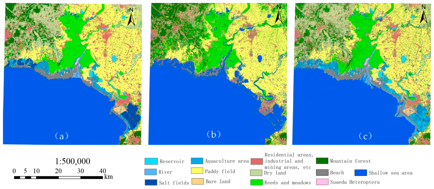
The year 2007 was selected as the benchmark for method comparison for the following reasons: (1) it has the largest number of training samples (723), allowing the classifiers to be more fully trained; (2) it includes all 13 landscape classes, ensuring complete class representation; (3) it falls within a period of policy adjustment, during which the area distribution among classes is relatively balanced, thus avoiding the influence of extreme class imbalance on accuracy assessment. Other years were not subjected to the same level of detailed comparison, but the same classification workflow and parameter settings were applied. Using 2007 as the benchmark year, landscape classification results obtained by the single MLC, single DT, and integrated MLC & DT methods are shown in Figure 4 and Table 6.

Figure 4. Classification results of 2007 were compared by DT (a), MLC (b), and MLC & DT (c).

Table 6. Results of the Three Classification Methods (Using 2007 as the Benchmark Year).

Classification Methods	Overall Accuracy (%)	Kappa Coefficient	Remarks
Single MLC method	75.29	0.71	Baseline method
Single DT method	56.82	0.57	Cannot achieve classification into all 13 categories
Integrated MLC & DT method	87.71	0.85	The method proposed in this study

Single MLC method: Overall accuracy is 75.29% with a Kappa coefficient of 0.71. There are obvious errors in the classification results. For example, upland dry land areas are often misclassified as reed due to similar spectral characteristics, and confusion among spectrally similar land-cover types is significant.

Single DT method: Overall accuracy is 56.82% with a Kappa coefficient of 0.57. This method fails to achieve detailed classification into all 13 classes and can only distinguish broad categories such as water & non-water. Major confusions are observed between forest land and dry land, paddy fields and reed, and bare land and residential areas.

Integrated MLC & DT method: The overall accuracy reaches 87.71% with a Kappa coefficient of 0.85, representing improvements of 16.50% and 19.72% over the single MLC method, and 54.36% and 49.12% over the single DT method, respectively.

These results indicate that the integrated approach effectively combines the strengths of both classifiers: MLC ensures baseline accuracy, while DT incorporates multi-source information as auxiliary input. Feature parameters further enhance spectral separability, making the method suitable for fine classification of complex and heterogeneous wetlands.

3.2. Coastline Changes

The coastal zone is a transitional area between wetland ecosystems and the marine environment, and its spatial position and morphological changes directly reflect the evolution of wetland patterns. The Liaohe Delta, as a typical silty estuarine wetland, exhibits coastline changes that are closely associated with the shrinkage of natural wetlands and the expansion of artificial wetlands. These changes serve as important indicators for revealing the intensity of human activities and the response of wetland ecosystems.

The natural coastline of the Liaohe Delta estuary region includes river ports and silty coastlines, and the artificial coastlines include the aquaculture dike coastlines, salt field dike coastlines, construction dike coastlines and port coastlines. The river port lines are determined based on the first road, bridge, or gate met by the estuary area from the sea direction landward. Due to the sudden widening of the estuary along the river, silty shorelines are generally located along this estuary and form the dividing line between the lushness and sparseness of the plants in the images [47]; the outer edge of this artificial shoreline is used as the dike line. Therefore, the tidal-flat and shallow-sea areas were set to intertidal zone, while the other classifications were set to terrestrial, meaning that each of the 13 classifications were classified into 2 categories and that the boundary between these two categories was the coastline.

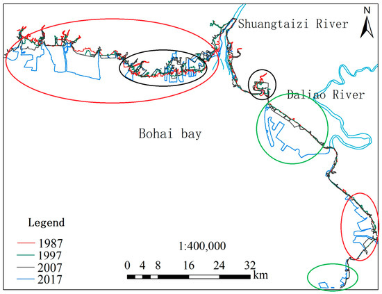
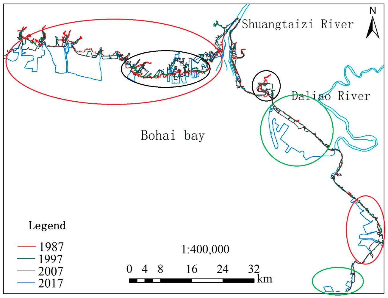
Coastlines were automatically extracted from the 1987, 1997, 2007, and 2017 images (Figure 5). The coastline extracted from the 2017 image was compared with the 2017 coastline released in the 2019 National Geographic Information Resource Directory Service System (NGIRDSS). It shows that from 1987 to 2017, the land area of the Liaohe Delta coastline increased by 263.24 km², and the coastline length in 2017 was approximately 329.886 km, reflecting an increase of 92.294 km compared to the 1987 coastline length. The temporal analysis shows that the land area increased by 171.30 km² from 1987 to 1997 (an average of 17.13 km² per year). From 1997 to 2007, it increased by 43.21 km² (an average of 4.32 km² per year), and from 2007 to 2017, it increased by 48.73 km² (an average of 4.87 km² per year). The average annual growth rate during 2007–2017 is 1.13 times that of 1997–2007, indicating a renewed intensification of human disturbance in recent years.

Figure 5. Coastline changes from 1987 to 2017.

Coastline changes in the Liaohe Delta show strong spatial differentiation. It shows that the silty coastline has been converted into aquaculture ponds and salt fields in the red-circled area, with an area transformation of approximately 45.3 km². In the green-circled area, the coastline has been converted into port shoreline and construction embankments, resulting in an increase of 23.6 km of artificial shoreline. In the black-circled area, erosion occurred from 1987 to 2007, but from 2007 to 2017, the area in the large black circle basically developed into an aquaculture area (32.8 km²), while that in the small black circle developed into a paddy field (8.5 km²).

3.3. Dynamic Changes in Landscape Area

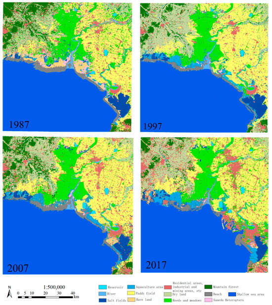
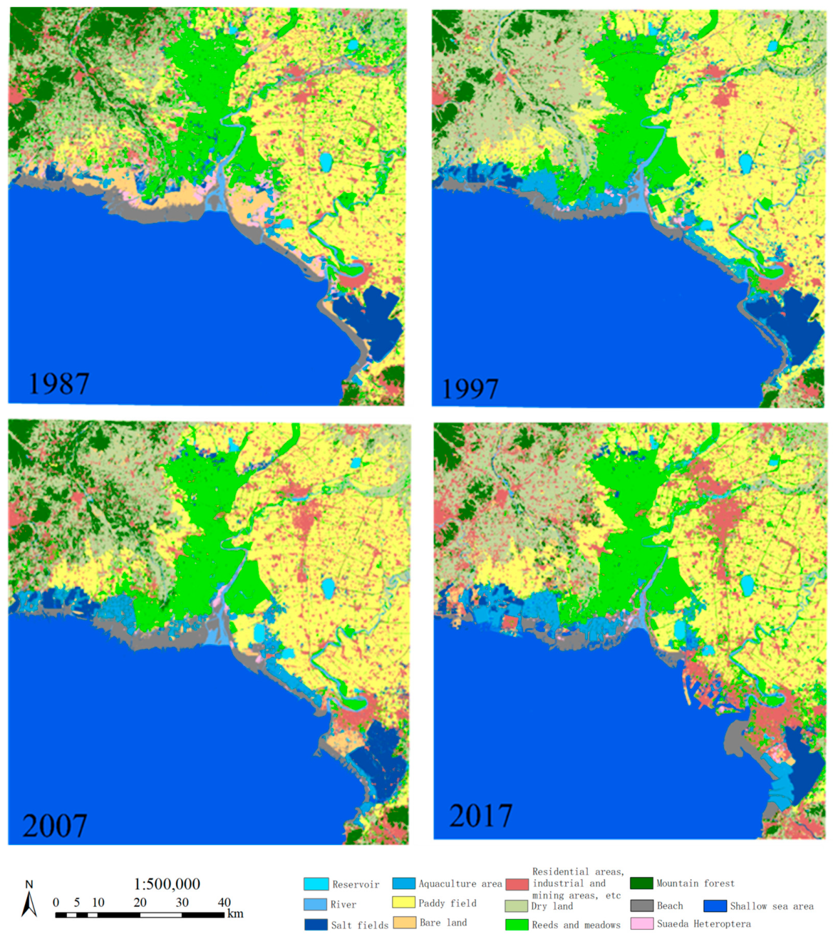
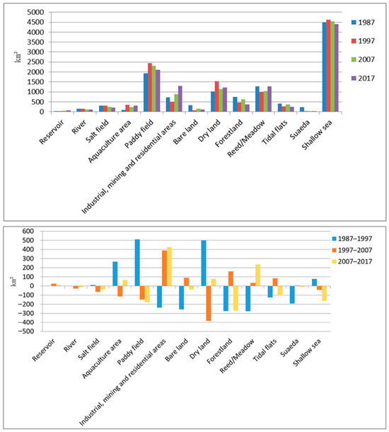
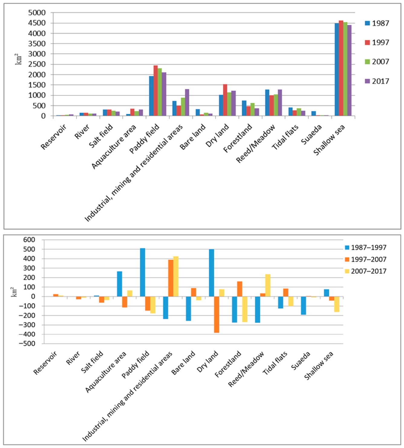
In 1987, the total area of the study region (excluding shallow sea areas) was 7287.25 km². Among this, the total wetland area was 2834.78 km², accounting for 38.9%, including 2403.29 km² (33.0%) of natural wetlands and 431.49 km² (5.9%) of constructed wetlands. Non-wetland areas covered 4452.47 km², representing 61.1% of the total area. Figure 6 shows the extraction results obtained for 1987, 1997, 2007, and 2017. Figure 7 shows the statistical histograms obtained for various types of land areas.

Figure 6. Landscape distribution map of the Liaohe Delta in 1987, 1997, 2007 and 2017.

Figure 7. Landscape area change of the Liaohe Delta in 1987, 1997, 2007 and 2017.

3.3.1. Changes in Wetland Area

It shows that large areas of reed lands were mainly distributed along the Shuangtaizi River. The area of reed meadow was approximately 1284.44 km² in 1987. However, this area was reduced to 1006.70 km² from 1987 to 1997. Then it recovered to 1040.20 km² in 2007 and further increased to 1275.53 km² in 2017, essentially returning to the 1987 level. From 1987 to 2017, it decreased by 0.69% overall (Table 7).

Table 7. Statistics of landscape area in wetland areas (km²).

Landscape Types	1987	1997	2007	2017	1987–2017	Rate of Change (%)
Reed/Meadow	1284.44	1006.70	1040.20	1275.53	−8.91	−0.69
Suaeda	227.48	35.23	39.70	30.52	−196.96	−86.58
Tidal flats	219.89	142.35	219.12	178.80	−41.09	−18.69
Aquaculture area	91.63	358.11	242.39	307.93	216.30	+236.06
Salt field	309.60	315.47	251.86	212.79	−96.81	−31.27
Reservoir	34.68	35.46	59.99	70.70	36.02	+103.86
Bare land	330.39	73.22	162.47	123.48	−206.91	−62.63
River area	156.32	154.88	126.26	113.68	−42.64	−27.28

Suaeda grows in saline–alkali soil and often forms single colonies on beaches and lakes. The area of Suaeda is decreasing annually in the study area. In 1987, this area was approximately 227.48 km². In 1997, it was reduced to 35.23 km², exhibiting a reduction rate of 84.51%. It slightly increased to 39.70 km² in 2007, then declined again to 30.52 km² in 2017. From 1987 to 2017, it decreased by 86.58% overall.

As a kind of intertidal zone between sea and land areas, tidal flats are affected by both the sea tide level and the local activities. It shows that from 1987 to 1997, large areas of tidal flats were transformed into aquaculture areas, decreasing from 219.89 km² in 1987 to 142.35 km² in 1997, indicating a significant declining trend. By 2007, the area rebounded to 219.12 km² due to two reasons: the Suaeda areas were transformed into tidal flats, and a certain degree of seawater erosion occurred along the shoreline from 1997 to 2007, thus increasing exposure and causing tidal flats to form. However, it declined again by 2017. An overall decrease of 18.69% was observed over the past 30 years. The natural intertidal ecosystem is subject to persistent pressure.

The aquaculture area changed significantly throughout the study period. In 1987, aquaculture areas were only sparsely distributed, covering approximately 91.63 km², and then expanded rapidly to reach 358.11 km² by 1997. In 2007, the number of aquaculture areas on land decreased, and the overall aquaculture area was reduced to 242.39 km²; the aquaculture industry in the coastal zone was revitalized by 2017, and some salt fields were even converted into aquaculture areas, resulting in an overall aquaculture area of 307.93 km².

In the study area, the area of salt fields basically showed a decreasing trend year by year. The area of salt fields was approximately 309.60 km² in 1987, and slightly increased to 315.47 km² in 1997. That is, the area of salt fields basically remained stable from 1987 to 1997, but then started to decrease to 251.86 km² in 2007 and further to 212.79 km² in 2017, representing a decline of 31.27%. Traditional salt production has gradually given way to aquaculture.

The area of reservoirs in the study area shows a continuous increase, rising from 34.68 km² in 1987 to 70.70 km² in 2017 with an increase of 103.86%, reflecting growing demand for regional water resource regulation. Bare land shows an overall decreasing trend. From 1987 to 2017, it decreased from 330.39 km² to 123.48 km² with a reduction rate of 62.63%. But the river area shows a decreasing trend, which is associated with reduced precipitation, upstream water interception, and increased water consumption.

3.3.2. Changes in Non-Wetland Area

The area of paddy fields was approximately 1936.71 km² in 1987. Due to the intensification of human activities, the paddy field area increased significantly to 2448.71 km² in 1997, reflecting an increase of approximately 512 km² and a growth rate of 26.44%. However, this area decreased annually in the later period. Industrial and mining areas and construction lands expanded significantly throughout the study period, occupying a large area previously occupied by rice fields. However, this area decreased to 2298.99 km² in 2007 and to 2120.20 km² in 2017 (Table 8). In short, the area of paddy fields showed a small trend in which it first increased and then decreased before demonstrating a steady decreasing tendency in the later period.

Table 8. Statistics of landscape area in non-wetland areas (km²).

Landscape Types	1987	1997	2007	2017	1987–2017	Rate of Change (%)
Paddy field	1936.71	2448.71	2298.99	2120.20	183.49	+9.47
Dry land	1028.60	1529.79	1146.49	1223.55	194.95	+18.95
Forestland	754.84	478.58	638.16	367.45	−387.39	−51.32
Industrial and mining buildings and residential areas	732.40	494.11	882.38	1307.31	574.91	+78.50

The area of dry lands increased year by year. In 1987, the dry land area was approximately 1028.60 km². However, in 1997, the dry land area was as high as 1529.79 km², reflecting a growth rate of 48.72%. Later, because of the conversion of a portion of these dry lands into rice fields and woodlands, the dry land area decreased. By 2017, the dry land area was approximately 1223.55 km², exhibiting a growth rate of approximately 18.95% compared to the 1987 area.

The area of “industrial and mining buildings and residential areas” was approximately 732.40 km² in 1987, but in 1997, this area was reduced to 494.11 km². The main reason for this decrease was that large areas lacking buildings and meadows in 1987 and earlier were considered among these areas. However, this area expanded from 882.38 km² (2007) to 1307.31 km² (2017), showing an increase of 574.91 km² over the past 30 years, with a growth rate of 78.50%.

Forestland shows an overall decreasing trend. From 1987 to 2017, forestland declined from 754.84 km² to 367.45 km², decreasing by 51.32%. It indicates a significant degradation of natural vegetation cover.

Therefore, because human activities have intensified, land use types such as residential areas, industrial and mining construction lands, and dock lands have appeared in the coastal areas; moreover, the coastal zone has continued to expand into the shallow-sea area. Throughout the study period, the Liaohe Delta area as a whole showed a trend in which the area of constructed wetlands expanded annually, the area of natural wetlands decreased, and a trend reflecting the internal transfer of non-wetland areas appeared.

3.4. Analysis of Landscape Transition Characteristics

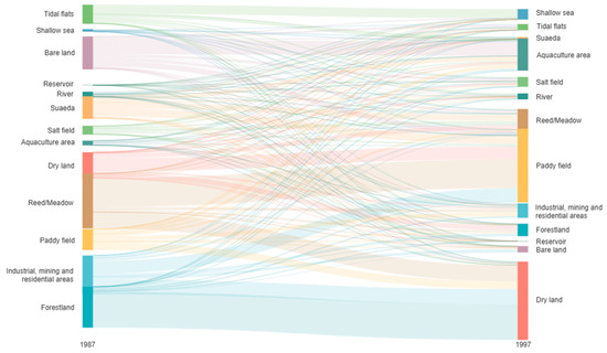
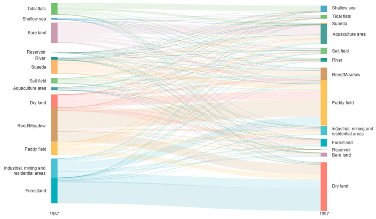
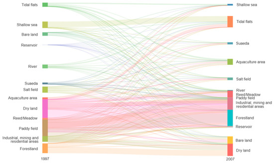
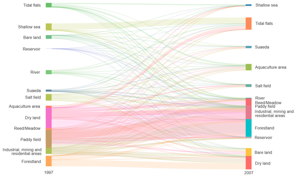
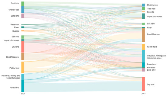
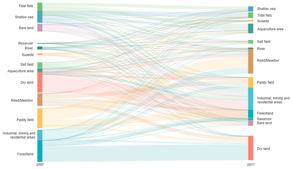
The study used Sankey diagrams to illustrate the main flows of landscape transitions (Figure 8, Figure 9 and Figure 10), replacing traditional transition matrix tables and thereby enhancing readability. The transitions of wetland landscape types are described across three periods.

Figure 8. Sankey diagram of landscape transition areas from 1987 to 1997.

Figure 9. Sankey diagram of landscape transition areas from 1997 to 2007.

Figure 10. Sankey diagram of landscape transition areas from 2007 to 2017.

(1) 1987–1997 (peak period of agricultural development)

During this period, landscape change was dominated by agricultural expansion, with substantial increases in paddy fields, dry land, and aquaculture areas. Detailed results are presented in Figure 8. Paddy fields increased by approximately 512 km², receiving 713.25 km² from other landscape types and losing 201.26 km² to other categories. It mainly converted from reed meadow, dry land, and bare land, with areas of 279.36 km², 125.61 km², and 54.88 km². Dry land increased by 501.20 km², with 759.26 km² converted from other landscape types and 258.06 km² transferred out. The major contributors were forest (347.49 km²); reeds and meadows (156.85 km²); and industrial, mining buildings and residential areas (146.22 km²). Aquaculture areas expanded by 266.50 km², mainly converted from bare land and Suaeda, accounting for 140.09 km² and 40.94 km², respectively. In contrast, reeds and meadows; forestland; bare land; industrial, mining buildings and residential areas; Suaeda; and tidal flats decreased sharply by 277.73 km², 276.26 km², 257.17 km², 238.19 km², 192.27 km², and 126.07 km², respectively. Salt fields, reservoirs, and rivers remained relatively stable.

(2) 1997–2007 (structural adjustment period)

During this period, landscape change was characterized primarily by urban expansion. The area of industrial, mining buildings and residential areas increased by 388.36 km², mainly converted from paddy fields and dry land, with transition areas of 170.73 km² and 149.63 km², respectively. Forestland and tidal flats increased by 159.71 km² and 129.21 km², mainly due to conversions from dry land and shallow sea areas. The expansion of tidal flats was primarily driven by marine erosion, which exposed new intertidal zones. Reed and meadow increased by 33.49 km², mainly converted from paddy fields and dry land. In contrast, dry land, paddy fields, and aquaculture areas decreased significantly, by 383.05 km², 149.45 km², and 115.69 km², respectively. Shallow sea areas, salt fields, and rivers all showed slight declines, while Suaeda remained relatively stable. Detailed results are presented in Figure 9.

(3) 2007–2017 (co-occurrence period of ecological restoration and urbanization)

During this period, urbanization continued to intensify, while the effects of ecological restoration policies became increasingly evident. The area of industrial, mining buildings and residential areas increased by 424.93 km², mainly converted from dry land and paddy fields, with transition areas of 152.27 km² and 115.95 km². It also expanded into the coastal zone, occupying 36.12 km² of tidal flats and 44.62 km² of shallow sea areas. Overall, the transition pattern remained broadly consistent with that observed during 1997–2007. Reed and meadow increased by 235.33 km², with 205.18 km² converted from paddy fields, largely driven by the “returning farmland to reed wetlands” policy. In contrast, forestland, paddy fields, shallow sea areas, and tidal flats decreased significantly by 270.71 km², 178.79 km², 132.72 km², and 131.53 km², mainly transitioning to dry land, reed and meadow, tidal flats, and aquaculture areas. Dry land and aquaculture areas showed slight increases, while salt fields and bare land experienced slight declines. The areas of Suaeda, rivers, and reservoirs remained relatively stable. Detailed results are presented in Figure 10.

4. Discussion

4.1. Method Positioning and Limitations

The integrated method proposed in this study (Kappa = 0.85) achieves improved accuracy within the MLC–DT framework; however, its comparison with more advanced methods remains limited. Methods mentioned in the introduction, such as object-based SVM (Kappa = 0.84–0.89) and Random Forest (Kappa = 0.83–0.87), have been reported in the literature to yield high accuracy. Nevertheless, no rigorous comparison under equivalent conditions (i.e., the same study area and validation samples) was conducted in this study. Therefore, within the MLC–DT integration framework, feature optimization and classifier combination can lead to accuracy improvements.

The advantages of the proposed method are as follows: (1) high computational efficiency, without requiring a large number of training samples; (2) strong interpretability, with explicit DT rules; (3) suitability for long-term time series analysis due to stable parameter settings. However, it also has some limitations: (1) its capability in handling high-dimensional feature spaces is inferior to that of deep learning methods; (2) feature parameter selection relies on experience, with a relatively low level of automation.

There remains considerable room for improvement. Future work will focus on: (1) introducing advanced methods such as Random Forest (RF) and Extreme Gradient Boosting (XGBoost) for comparison under equivalent conditions; (2) exploring optimization strategies for deep learning approaches (e.g., U-Net) in fine classification of 13 classes; (3) developing adaptive feature selection algorithms to reduce manual intervention.

4.2. Typological Differentiation and Stability of Wetland Landscape Change

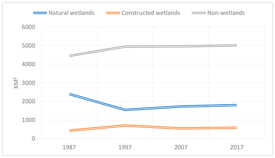
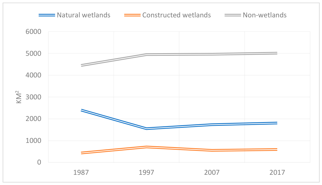
In the Liaohe Delta region, an area containing natural wetlands including rivers, reeds, suaeda, and tidal flats generally first declined and then increased throughout the study period (Figure 11). Among the land types, the river area decreased annually, mainly due to the decreasing precipitation, the decreasing river water level and the encroachment of the riverbanks, tidal flats and meadows. Although reed wetlands were destroyed by anthropogenic activities from 1987 to 1997, thus greatly reducing their area, the reed wetland area was effectively repaired in the later period. By 2017, this area was basically the same as that in 1987, which differs from the analysis results of Li [36]. The area of Suaeda decreased year by year and was mainly transformed into aquaculture areas, paddy fields, and reed meadows. In general, Suaeda was affected by human activities and greatly reduced throughout the study period. The tidal flats were developed into aquaculture areas and salt fields as a result of human activities; on the other hand, large areas of new tidal flats formed due to the impact of seawater erosion, but the overall area generally decreased.

Figure 11. Change trend of the first class classification of the Liaohe Delta.

Constructed wetlands showed an overall trend of first declining and then growing; these regions mainly included salt fields, aquaculture areas, and reservoirs. The salt field area increased from 1987 to 1997, but continuously decreased in the later period. Aquaculture was vigorously developed in 1997. Although the aquaculture area decreased in the later period, it remained relatively stable. The reservoir area increased year by year and was basically consistent with the analysis results of Liu and Ji [37,48].

Non-wetland areas occupied a large expanse and showed an increasing trend year by year. The main types of non-wetlands included paddy fields, forestland, dry land, industrial and mining buildings and residential areas. In addition to the mutual transformation among rice fields, dry lands and reed meadows, a mutual transformation relationship was observed among the non-wetland areas; this was mainly reflected in the conversions of rice fields, dry lands, and forestlands to industrial and mining buildings and residential areas and in the mutual transformations among rice fields, dry lands, and forestlands. The industrial and mining buildings and residential areas increased throughout the study period, while the area of forestland decreased [36].

However, during the classification process, this study classified cattail meadows and deer meadows as reeds, shrub meadows as forestlands, and tamarisk-tamame meadows as bare lands. Areas without buildings and meadows were classified as construction lands. Although there was no problem with the above classification scheme in terms of the land use types, and all land use types were either natural wetlands or non-wetlands, a technicality remains to be discussed.

4.3. Correlation Analysis Between Coastline Changes and Wetland Dynamics

There is a spatial association between shoreline change and wetland type transitions. The expansion of artificial shorelines spatially overlaps with the reduction in tidal flats, while along the coast there has been notable growth in port shorelines, embankment construction, aquaculture, and paddy fields. Because tidal effects were not considered, some “shoreline changes” may be pseudo-changes. For example, the image from 28 September 2007 was acquired during a spring tide, whereas the image from 7 September 2017 corresponds to a mid-tide period. Differences in tidal levels may have caused shoreline extraction offsets of 100–200 m, contributing approximately 15–30 km² of apparent “land increase.” Nevertheless, this does not alter the fact that the shoreline has been significantly modified by human activities.

4.4. Analysis of the Driving Mechanisms of Climate Change and Land Use

4.4.1. Indirect Effects of Climatic Factors

The Liaohe Delta is characterized by a warm temperate continental semi-humid monsoon climate with high rate of change in precipitation. Between 1987 and 2017, regional annual precipitation exhibited a fluctuating downward trend, decreasing by approximately 12–15%. This declining precipitation trend is consistent with the direction of river shrinkage, suggesting that climatic factors may have contributed partially to the observed changes.

However, climate forcing alone is insufficient to explain the magnitude and direction of key turning points. For example, the rapid expansion of paddy fields and dry land in 1997 (increasing by 512 km² and 501 km², respectively) coincided precisely with the implementation period of the Liaohe Delta Agricultural Comprehensive Development policy during 1995–2000. Similarly, the rapid recovery of reed wetlands after 2003 coincides with the implementation period of the “Returning Farmland to Reed Wetlands” policy. This indicates that policy-driven land-use change exerted a much stronger influence on wetland landscape patterns than natural climatic factors.

4.4.2. Direct Drivers of Land-Use Change

Wetland evolution in the Liaohe Delta was closely associated with human activities and exhibited a three-tiered progressive structural pattern from 1987 to 2017.

First level: Agricultural restructuring (1987–1997). Large-scale land reclamation driven by grain production reached its peak. A total of 626 km² of natural wetlands and forest land was converted into cropland, representing the highest intensity of ecological encroachment by agricultural development over the 30-year period. This stage is closely associated with government-led agricultural policies.

Second level: Industrialization and urbanization (1997–2017). The area of industrial, mining, and residential land increased by 78.5%, occupying substantial areas of cropland, including 115.95 km² of paddy fields and 152.27 km² of dry land, and extending into coastal zones, where it encroached upon 36.12 km² of tidal flats and 44.62 km² of shallow sea areas. Port and harbor construction led to the proportion of artificial coastline increasing from 12.4% to 38.7%, resulting in a significant loss of natural coastal characteristics. This stage was primarily driven by land value enhancement under market forces.

Third level: Industrial economic transformation (2007–2017). The conversion of salt fields into aquaculture areas and the upgrading of traditional agriculture into high-efficiency aquaculture reflect land-use optimization driven by market-oriented economic mechanisms. The interaction between policy regulation and market forces became the dominant feature of this phase.

4.5. Comparison of Global Deltas and Regional Specificity

Examining the Liaohe Delta within the global context of delta wetland change helps to identify both its unique characteristics and shared patterns (Table 9) [49,50,51,52,53]. Comparative analysis shows that the rate of natural wetland loss in the Liaohe Delta is at a moderate level globally, but it exhibits three salient features.

Table 9. Comparative analysis of wetland changes in major global deltas.

Delta	Study Period	Natural Wetland Change (%)	Dominant Driving Factors	Coastline Change Characteristics
Liaohe Delta	1987–2017	−13.7	Policy–market dual-driven	Rapid increase in artificial coastlines and degradation of natural coastlines
Yangtze River Delta	1980s–2015	−22.3	Land reclamation-driven	Large-scale conversion of tidal flats to agriculture and aquaculture
Yellow River Delta	1976–2016	−18.5	River course shifts and development	Rapid conversion of newly formed sediments into oilfields and farmland
Mekong Delta	1973–2013	−15.0	Hydropower development and agriculture	Sediment deficiency leading to coastal erosion
Ganges–Brahmaputra Delta	1973–2014	−12.0	Population pressure	Expansion of embankments and reduction in floodplains
Mississippi River Delta	1932–2000	−35.0	Engineering control	Levee construction and wetland subsidence

(1) A “bipolar” restoration pattern. Unlike the Yangtze River Delta (characterized by continuous degradation) and the Mississippi River Delta (dominated by engineering-induced degradation), the Liaohe Delta exhibits a pattern of simultaneous inland recovery and coastal degradation. After 2003, reed wetland area increased by 26.8%, representing a positive case among global deltas; however, the coastal Suaeda wetlands experienced severe degradation of 86.6%, indicating extreme degradation. This spatial divergence reflects the scale dependency of policy effects. Inland conservation policies have been effective, while coastal zone management remains insufficient.

(2) The “substitutional expansion” of artificial wetlands. Global deltas commonly experience the conversion of natural wetlands into non-wetland land uses, such as agriculture and urban areas. In contrast, a salient feature of the Liaohe Delta is the transformation of natural wetlands into constructed wetlands, for example, the conversion of tidal flats into aquaculture ponds and salt pans into aquaculture areas. The proportion of artificial wetlands increased from 5.9% to 18.2%. This form of “artificial substitution” has helped maintain certain ecological functions (e.g., providing habitats for water birds), while simultaneously altering the natural characteristics of wetlands.

(3) Policy–market dual-driven mechanism. Unlike the Mekong Delta (dominated by upstream hydropower development) and the Mississippi River Delta (controlled primarily by engineering interventions), changes in the Liaohe Delta are jointly driven by policy regulation (e.g., returning farmland to reed wetlands and nature reserve establishment) and market forces (e.g., aquaculture profitability and land value appreciation). The spatiotemporal coupling of these two drivers has generated a complex trajectory of landscape evolution.

4.6. Integrated Effects of Wetland Ecosystem Change and Management Implications

Over the past 30 years, wetland evolution in the Liaohe Delta has been characterized by a general pattern of “natural wetlands becoming artificialized, constructed wetlands becoming industrialized, and non-wetland areas becoming urbanized.” Consequently, ecosystem service functions have undergone qualitative changes.

(1) Maintenance functions. The flood regulation and water purification functions of reed wetlands have been largely maintained, as their area has remained relatively stable. However, the biodiversity-supporting function of Suaeda wetlands has severely degraded, with an 86.6% reduction in area and the loss of habitats for species such as the black-faced spoonbill. (2) Regulating functions. The carbon sequestration capacity of tidal flats has been weakened due to land reclamation, with natural tidal flat areas decreasing by 35.2% and sediment burial efficiency declining. (3) Cultural functions. The tourism value of the “Red Beach” landscape has been undermined by the degradation of Suaeda heteroptera wetlands, with its area reduced to 1.33 km² in 2018, thereby negatively affecting regional ecotourism development. However, following the implementation of local government policies, ecological conditions have been substantially restored, and by 2023 the area of Suaeda has expanded to 16.67 km² [54].

This study yields several management implications for the Liaohe Delta. (1) An ecological redline should be established in coastal zones to restrict the unregulated expansion of artificial shorelines. Based on the analysis in this study, the protection of natural wetlands within a 3 km coastal buffer zone should be prioritized as a key regulatory area. (2) Tidal flat hydrological connectivity should be restored. Measures such as removing abandoned aquaculture embankments and constructing ecological dikes can facilitate the natural recovery of Suaeda communities and help break the positive feedback loop of “shoreline hardening–wetland degradation.” (3) The industrial structure should be optimized to balance economic benefits and ecological functions. Ecological aquaculture models should be promoted, and a certain proportion of natural habitat patches should be retained within artificial wetlands to maintain the connectivity of the wetland network.

5. Conclusions

In this paper, referring to the existing wetland classification system and by comprehensively considering the characteristics of the Liaohe Delta wetland, a three-level classification system for coastal wetland landscapes in the Liaohe Delta region was established. This study developed an integrated classification framework combining MLC and DT, and optimized feature parameter selection. Landsat remote sensing images taken on 4 instances in 1987, 1997, 2007, and 2017 were used to extract landscape information and landscape dynamic change information to perform a quantitative analysis of wetland and coastline change characteristics. The following conclusions were obtained in this work:

(1) Methodological contributions and limitations: The integrated MLC–DT approach achieved an overall accuracy of 87.71% and a Kappa coefficient of 0.85, indicating improved classification performance within the MLC–DT framework. However, the advantages of this method require further rigorous validation through comparisons with more advanced approaches such as object-based analysis, SVM, and Random Forest under comparable conditions. The current results can nevertheless support long-term wetland monitoring and time-series analysis.

(2) Evolution patterns: From 1987 to 2017, the wetlands of the Liaohe Delta exhibited a bipolar pattern of “inland recovery and coastal degradation.” Reed and meadow wetlands recovered to near baseline levels, whereas Suaeda wetlands declined by 86.6%, and tidal flats continued to shrink. Although the coastline advanced landward by 263.24 km², this estimate should be interpreted with caution due to tidal variability and associated uncertainties.

(3) Driving factors: Landscape changes are temporally associated with the implementation of conservation policies; however, causal inference requires additional independent evidence. Human activities can be identified as the dominant driving force in terms of directionality, but the relative contributions of individual factors have not yet been quantified.

(4) Management recommendations: It is recommended to establish a coastal ecological redline, restore tidal flat hydrological connectivity, and optimize the industrial structure. Future research should be conducted using more detailed datasets, including high-resolution remote sensing imagery, tidal models, and socio-economic statistics.

References

- Lu, X.; Wang, R. Study on wetland biodiversity in China. Chin. Geogr. Sci. 1996, 1, 15–23. [Google Scholar] [CrossRef] [Scilit]
- Liu, R.; Liang, S.; Zhao, H.; Qi, G.; Li, L.; Jiang, Y.; Niu, Z. Progress of Chinese coastal wetlands based on remote sensing. Remote Sens. Technol. Appl. 2017, 32, 998–1011. [Google Scholar]
- Chen, L.; Ren, C.; Zhang, B.; Li, L.; Wang, Z.; Song, K. Spatiotemporal dynamics of coastal wetlands and reclamation in the Yangtze Estuary during past 50 years (1960s–2015). Chin. Geogr. Sci. 2018, 28, 386–399. [Google Scholar] [CrossRef] [Scilit]
- Jin, Y.; Gao, J.; Zhou, K.; Mu, S. Dynamic of land use/cover changes under reclamation and Spartina alterniflora invasion in Jiangsu central coastal wetlands. Geogr. Res. 2017, 36, 1478–1488. [Google Scholar]
- Wu, X.; Wang, H.; Bi, N.; Nittrouer, J.A.; Xu, J.; Cong, S.; Carlson, B.N.; Lu, T.; Li, Z. Evolution of abandoned deltaic river channel—A case from the Diaokou channel of the Yellow River. Mar. Geol. Quat. Geol. 2021, 41, 22–29. [Google Scholar] [CrossRef]
- Yang, H.; Qiao, L.; Liu, X.; Zhang, Y.; Wang, P.; Chen, X. Shoreline evolution of the Red River Delta in the recent 30 years. Mar. Geol. Quat. Geol. 2020, 40, 48–57. [Google Scholar] [CrossRef]
- Yan, F.; Liu, X.; Chen, J.; Yu, L.; Yang, C.; Chang, L.; Yang, J.; Zhang, S. China’s wetland databases based on remote sensing technology. Chin. Geogr. Sci. 2017, 27, 374–388. [Google Scholar] [CrossRef] [Scilit]
- Liu, X.; Liu, H.; Lin, Z.; Jia, J.; Lv, S. Comparisons of classification methods for coastal wetlands in Yancheng City based on Landsat OLI images. Wetl. Sci. 2017, 15, 689–696. [Google Scholar] [CrossRef]
- Zhou, X.; Wang, Y.; Liu, S.; Yu, P.; Wang, X. A machine learning algorithm for automatic identification of cultivated land in remote sensing images. Remote Sens. Land Resour. 2018, 30, 68–73. [Google Scholar]
- Wu, W.; Zhang, Y.; Li, Q.; Huang, H. A hierarchical classification and iterative model based method for remote sensing classification of land cover. Remote Sens. Technol. Appl. 2019, 34, 68–78. [Google Scholar]
- Jiang, J.; Wen, X.; Wang, H.; Yu, G.; Lin, G. Extraction and dynamic change analysis of coastal wetland type information in Yancheng over the past decade. J. Northwest For. Univ. 2019, 34, 167–173. [Google Scholar]
- Xiao, J.; Ou, W.; Fu, H. Land cover classification of Yancheng coastal natural wetlands based on BP neural network and ETM+ remote sensing data. Acta Ecol. Sin. 2013, 33, 7496–7504. [Google Scholar] [CrossRef] [Scilit]
- Radman, A.; Mohammadimanesh, F.; Mahdianpari, M. Wet-ConViT: A Hybrid Convolutional–Transformer Model for Efficient Wetland Classification Using Satellite Data. Remote Sens. 2024, 16, 2673. [Google Scholar] [CrossRef] [Scilit]
- Zhang, X.; Du, L.; Tan, S.; McCarty, G.W.; Zou, Z. Wetland classification based on depth-adaptive convolutional neural networks using leaf-off SAR imagery. Sci. Total Environ. 2024, 957, 177768. [Google Scholar] [CrossRef] [Scilit]
- Turnbull, A.; Soto-Berelov, M.; Coote, M. Delineation and classification of wetlands in the Northern Jarrah Forest, Western Australia using remote sensing and machine learning. Wetlands 2024, 44, 52. [Google Scholar] [CrossRef] [Scilit]
- Liu, C.; Yuan, X.; Ni, G.; Liu, Y.; Qi, Y.; Miao, S. Utilizing deep transfer learning to discover changes in landscape patterns in urban wetland parks based on multispectral remote sensing. Ecol. Inform. 2024, 83, 102808. [Google Scholar] [CrossRef] [Scilit]
- Xu, Y.; Tao, X.; Ni, Z.; Liu, Z.; Fu, Y.; Ren, P. Material proportion guided hyperspectral image super-resolution via unmixing. ISPRS J. Photogramm. Remote Sens. 2026, 235, 584–598. [Google Scholar] [CrossRef] [Scilit]
- Effah, D.; Zia, A.; Awrangjeb, M.; Gao, Y.; Sarpong, K. Advances in machine learning for wetland classification: A comprehensive survey of methods and applications. Artif. Intell. Rev. 2026, 59, 24. [Google Scholar] [CrossRef] [Scilit]
- Zhou, L.; Yao, X.; Lu, X. Wetland land-cover information extraction using BP neural network based on tolerant rough set in Shuangtaizi Estuary wetland. Resour. Sci. 2016, 38, 1538–1549. [Google Scholar]
- Yao, Y.; Zhang, Z.; Qin, Q.; Qiu, Y. Study on wetland information extraction of remote sensing images based on support vector machine. Comput. Appl. Res. 2008, 4, 989–990. [Google Scholar]
- Li, H.; Huang, J.; Liang, Y.; Wang, H.; Zhang, Y.C. Evaluating ecological environment quality in Wuhan based on remote sensing ecological index. J. Yunnan Univ. Nat. Sci. Ed. 2020, 42, 81–90. [Google Scholar]
- Shi, T.; Wang, C.; Zhang, W.; He, J. Classification of coastal wetlands in the Liaohe Delta with multi-source and multi-feature integration. Environ. Monit. Assess. 2025, 197, 247. [Google Scholar] [CrossRef] [Scilit] [PubMed]
- Wang, Y.; Jin, S.; Dardanelli, G. Vegetation classification and evaluation of Yancheng coastal wetlands based on Random Forest algorithm from Sentinel-2 images. Remote Sens. 2024, 16, 1124. [Google Scholar] [CrossRef] [Scilit]
- Xing, H.; Niu, J.; Feng, Y.; Hou, D.; Wang, Y.; Wang, Z. A coastal wetlands mapping approach of Yellow River Delta with hierarchical classification and optimal feature selection framework. Catena 2023, 223, 106897. [Google Scholar] [CrossRef] [Scilit]
- Zhang, J.; He, Q.; Cui, T.; Shi, P.; Yang, T. Information extraction and dynamic changes of wetland in Jiangsu coastal area based on RS and GIS. J. Yangtze River Acad. Sci. 2017, 34, 144–150. [Google Scholar]
- Chang, X.; Dong, C.; Luo, M. Contrast analysis of supervised classification and decision tree method to extract Qinzhou Bay wetland. Chin. Agric. Sci. Bull. 2014, 30, 295–300. [Google Scholar]
- Sivakumar, R.; Ghosh, S. Wetland spatial dynamics and mitigation study: An integrated remote sensing and GIS approach. Nat. Hazards 2016, 80, 975–995. [Google Scholar] [CrossRef] [Scilit]
- Szantoi, Z.; Escobedo, F.J.; Abd-Elrahman, A.; Pearlstine, L.; Dewitt, B.; Smith, S. Classifying spatially heterogeneous wetland communities using machine learning algorithms and spectral and textural features. Environ. Monit. Assess. 2015, 187, 262. [Google Scholar] [CrossRef] [Scilit]
- Gu, X.; Gao, X.; Ma, H.; Wang, L.; Zhang, P. Comparison of machine learning methods for land use/land cover classification in complicated terrain regions. Remote Sens. Technol. Appl. 2019, 34, 57–67. [Google Scholar]
- Cui, L.; Zhang, J.; Wu, Z.; Xun, L.; Wang, X.; Zhang, S.; Bai, Y.; Zhang, S.; Yang, S.; Liu, Q. Superpixel segmentation integrated feature subset selection for wetland classification over Yellow River Delta. Environ. Sci. Pollut. Res. 2023, 30, 50796–50814. [Google Scholar] [CrossRef] [Scilit]
- Ke, L.; Tan, Q.; Lu, Y.; Wang, Q.; Zhang, G.; Zhao, Y.; Wang, L. Classification and spatio-temporal evolution analysis of coastal wetlands in Liaohe Estuary from 1985 to 2023. Front. For. Glob. Change 2024, 7, 1406473. [Google Scholar] [CrossRef] [Scilit]
- Qian, H.; Bao, N.; Meng, D.; Zhou, B.; Lei, H.; Li, H. Mapping and classification of Liao River Delta coastal wetland based on stacking ensemble model. Ecol. Inform. 2024, 80, 102488. [Google Scholar] [CrossRef] [Scilit]
- Xu, D.; Wu, W.; Ma, Y.; Feng, D. Research on wetland fine classification based on remote sensing images. Sustainability 2025, 17, 10900. [Google Scholar] [CrossRef] [Scilit]
- Zhang, L.; Wang, Z.; Wang, J.; Hu, Q.; Chang, Y.; Lu, Z.; Zhao, J. An integrated feature framework for wetland mapping using multi-source imagery. Remote Sens. 2025, 17, 3737. [Google Scholar] [CrossRef] [Scilit]
- Ma, G. Evaluation of Wetland Ecosystems of International Importance in China; Science Press: Beijing, China, 2016; pp. 209–216. [Google Scholar]
- Li, M.; Xu, L.; Wang, X.; Jia, K. The degradation analysis of reed and seepweed wetlands in Shuangtai Estuary reserve. Geom. Spat. Inf. Technol. 2020, 43, 99–103. [Google Scholar]
- Liu, T.; Liu, X.; Du, J.; Song, K. Pattern and change of coastal wetlands in Liaohe River Delta for five periods. Wetl. Sci. 2017, 15, 622–628. [Google Scholar] [CrossRef]
- Yin, X.; Hou, Y.; Wang, F. Dynamic change of land use in Liaohe Delta based on GIS. Territ. Nat. Resour. Study 2019, 2, 63–65. [Google Scholar] [CrossRef]
- Modica, G.; Solano, F.; Merlino, A.; Di Fazio, S.; Barreca, F.; Laudari, L.; Fichera, C.R. Using Landsat 8 imagery in detecting cork oak woodlands. J. Agric. Eng. 2016, 47, 205–215. [Google Scholar] [CrossRef] [Scilit]
- Almeida, T.I.R.; Penatti, N.C.; Ferreira, L.G.; Arantes, A.E.; Amaral, C.H. Principal component analysis applied to MODIS images: Pantanal wetland variability. Wetl. Ecol. Manag. 2015, 23, 737–748. [Google Scholar] [CrossRef] [Scilit]
- Liu, L.; Li, C.; Lei, Y.; Yin, J.; Zhao, J.; Sun, X. Feature extraction for hyperspectral image using weighted PCA-ICA. Arab. J. Geosci. 2017, 10, 307. [Google Scholar] [CrossRef] [Scilit]
- Yang, Z.; Bai, J.; Chen, Z.; Qian, X. Object-based wetland decision tree classification using Sentinel-2A image. J. Geomat. Sci. Technol. 2019, 36, 262–268. [Google Scholar]
- Xu, H. Fast information extraction of urban built-up land based on spectral signature and ND index. Geogr. Res. 2005, 2, 311–320. [Google Scholar]
- Zhang, H.; Zhang, Y.; Tian, M.; Wu, C. Dynamic monitoring of eco-environment quality changes based on PCA: Baoji City case. Remote Sens. Nat. Resour. 2018, 30, 203–209. [Google Scholar]
- Congalton, R.G. A review of assessing the accuracy of classifications of remotely sensed data. Remote Sens. Environ. 1991, 37, 35–46. [Google Scholar] [CrossRef] [Scilit]
- Congalton, R.G.; Green, K. Assessing the Accuracy of Remotely Sensed Data: Principles and Practices, 3rd ed.; CRC Press: Boca Raton, FL, USA, 2019. [Google Scholar]
- Wang, J.; Zhang, J.; Chen, J.; Liu, Y.; Li, F.; Sun, X. Analysis of Liaohe Estuary coastline changes using remote sensing images. Mar. Environ. Sci. 2015, 34, 86–92. [Google Scholar] [CrossRef]
- Ji, Y.; Zhou, G. Transformation of vegetation structure in China’s Liaohe Delta (1988–2006). Chin. J. Plant Ecol. 2010, 34, 359–367. [Google Scholar]
- Ma, X.; Du, J.; Liang, Y.; Zhang, D. Changes of coastal wetlands in the Yangtze River Delta for six periods since the 1960s and their driving factors. Wetl. Sci. 2018, 16, 303–312. [Google Scholar] [CrossRef]
- Zhang, B.; Zhang, Q.; Feng, C.; Feng, Q.; Zhang, S. Understanding land use and land cover dynamics from 1976 to 2014 in Yellow River Delta. Land 2017, 6, 20. [Google Scholar] [CrossRef] [Scilit]
- Zhou, K. Wetland landscape pattern evolution and prediction in the Yellow River Delta. Appl. Water Sci. 2022, 12, 190. [Google Scholar] [CrossRef] [Scilit]
- Chaiyana, A.; Immitzer, M.; Som-ard, J.; Khamkhon, R.; Kangrang, A.; Kaewplang, S.; Laongmanee, W.; Koedsin, W.; Vaiphasa, C.; Huete, A. Spatial and Temporal Patterns of Mangrove Forest Change in the Mekong Region over Four Decades Based on a Remote Sensing Data-Driven Approach. Remote Sens. 2025, 17, 3728. [Google Scholar] [CrossRef] [Scilit]
- Nicholls, R.J.; Hutton, C.W.; Adger, W.N.; Hanson, S.E.; Rahman, M.M.; Salehin, M. (Eds.) Ecosystem Services for Well-Being in Deltas: Integrated Assessment for Policy Analysis; Springer International Publishing: Cham, Switzerland, 2018. [Google Scholar] [CrossRef] [Scilit]
- Xinhua News. Available online: https://www.news.cn/photo/2023-07/19/c_1129757920.htm (accessed on 19 July 2023).
Disclaimer/Publisher’s Note: The statements, opinions and data contained in all publications are solely those of the individual author(s) and contributor(s) and not of MDPI and/or the editor(s). MDPI and/or the editor(s) disclaim responsibility for any injury to people or property resulting from any ideas, methods, instructions or products referred to in the content. |
© 2026 by the authors. Licensee MDPI, Basel, Switzerland. This article is an open access article distributed under the terms and conditions of the Creative Commons Attribution (CC BY) license.