Adaptive Extraction of the Main Axis of the Kuroshio Current in the Northwest Pacific and Analysis of Multiscale Variability Mechanisms in the Front Zone

Abstract

Accurately capturing the Kuroshio’s main axis and its multiscale frontal variations remains challenging due to the constraints of traditional fixed-section extraction methods. Here, we develop an adaptive iterative tracking algorithm utilizing high-resolution reanalysis data (2002–2024) that dynamically adjusts search directions and cross-sections via local velocity vectors, integrated with a dynamic step size and two-dimensional validation. Applying a multiscale variability decomposition framework across four key regions reveals distinct spatiotemporal dynamics. The North Equatorial Current bifurcation zone exhibits a significant strengthening trend driven by seasonal zonal and decadal meridional flows. Conversely, the Kuroshio east of Taiwan is dominated by high-frequency mesoscale processes (~70%) with a semi-annual cycle and no long-term trend. The East China Sea front maintains a highly stable seasonal meridional signal (25%). Crucially, the Luzon Strait intrusion shows a significant long-term weakening trend (~0.0029 m·s⁻¹·a⁻¹, p < 0.01), characterized by eastward strengthening and northward weakening, with ENSO significantly modulating its seasonal cycle. This approach substantially reduces systematic extraction errors compared to traditional fixed-section methods, as independently verified using satellite SST frontal gradients (median deviation < 0.2°), providing critical observational evidence for understanding western boundary current–marginal sea interactions and their dynamical responses under global warming.

1. Introduction

As the strong current forming the western boundary of the North Pacific subtropical circulation system, the Kuroshio is characterized by high flow velocity, strong baroclinicity, multiscale oscillations in its path, and nonlinear behavior. It is a major oceanic phenomenon that regulates the dynamic, thermal, and ecological processes in the northwest Pacific and the waters off the coast of China. The Kuroshio Front Zone, comprising the main axis of the Kuroshio Current and its adjacent high-gradient bands, is not only a key region for oceanic frontal processes, mesoscale eddy generation and dissipation, and air–sea interaction, but also serves as a link between the tropical Pacific and the mid-latitude shelf systems [1,2,3]. A deep understanding of the multiscale variability patterns and dynamical mechanisms of the Kuroshio Front Zone holds significant scientific and practical value for improving marine environmental forecasting capabilities, assessing coastal ecosystems and fishery resources, and predicting the response of marginal seas under global warming.

However, the precise identification of the Kuroshio Front and research into its variability mechanisms still face several challenges. First, traditional methods for extracting the Kuroshio’s main axis—including the maximum current velocity line method at fixed cross-sections [4], the hydrographic feature tracing method [5], and the geostrophic current main axis method using satellite altimeters [6]— have certain limitations: fixed cross-sections cannot adapt to the Kuroshio’s bending and oscillations; there is a phase difference between hydrographic fronts and the main axis of the flow field; geostrophic currents deviate from the actual flow field in nearshore and eddy-active regions; and threshold methods are prone to noise interference, leading to jagged discontinuities. These issues make it difficult for traditional methods to achieve high-precision, continuous, and automated extraction of the Kuroshio’s main axis, thereby limiting the reliability of subsequent variability analyses. Second, the variability of the Kuroshio front exhibits multi-scale superposition, spanning intra-seasonal [4], seasonal, interannual [7], and decadal [8] timescales. The Kuroshio branches off from the North Equatorial Current in its source region, passes through the main branch east of Taiwan and interacts with the East China Sea shelf, and intrudes into the marginal sea at the Luzon Strait; however, the dominant variability modes and driving mechanisms in each of these regions have yet to be systematically quantified.

To address these issues, this paper first proposes an adaptive iterative tracking algorithm based on flow field dynamics constraints to achieve precise, continuous, and automated extraction of the Kuroshio’s main axis. This algorithm uses local velocity vectors as dynamic constraints to adjust the tracking direction and search cross-section in real time, ensuring that the search cross-section remains perpendicular to the local instantaneous direction of the Kuroshio Current. Additionally, a dynamic step-size adjustment mechanism is introduced: the step size is increased in stable flow regions to enhance efficiency, and decreased in curved sections of the Kuroshio Current to ensure accuracy. A two-dimensional verification mechanism combining historical position and direction is established to effectively identify and correct anomalies such as positional stagnation and directional jumps, followed by smoothing via moving averages and cubic spline interpolation. This method eliminates systematic errors caused by preset cross-sections and fixed search directions, thereby enhancing the algorithm’s robustness against noise and its adaptability to complex paths. Building on this, this study adopts a multiscale variability decomposition framework for oceanic time-series flow velocities. First, the seasonal cycle of the climate mode is extracted via Fourier fitting of the first four harmonics to prevent seasonal signals from leaking into the trend component. Subsequently, a fourth-order Butterworth low-pass filter with zero-phase distortion is used to extract long-term low-frequency variability (period > 60 months), and boundary effects are eliminated through mirror extension. Further filtering yields the interannual anomaly component (24–60 months), with the remaining portion constituting high-frequency residuals (<24 months). Concurrently, variance contribution decomposition (allocating non-orthogonal components based on the covariance matrix), Mann–Kendall trend tests with autocorrelation correction, and Morlet wavelet red noise spectral analysis are combined to analyze the energy distribution, long-term trends, and periodic characteristics of current velocity variability in the Kuroshio Front. Due to the limited length (2002–2024) of the reanalysis data, decadal signals longer than approximately 10–12 years cannot be statistically resolved as stable periodic cycles. Therefore, the low-frequency component extracted by the 60-month low-pass filter is interpreted as low-frequency variability (including possible multi-year to decadal fluctuations) rather than strictly periodic decadal oscillations.

This study selected four key sections along the main axis of the Kuroshio Current for comparative analysis: the North Equatorial Current bifurcation zone in the North Pacific (Kuroshio source region), the Kuroshio front east of Taiwan (main transport segment), the Kuroshio front in the East China Sea (shelf interaction segment), and the Kuroshio intrusion zone in the Luzon Strait (marginal sea penetration segment). Spatially, these four regions constitute a complete chain of the Kuroshio from its origin, transport, and shelf interaction to its penetration into the marginal sea; dynamically, they cover all key stages of the Kuroshio’s multiscale variability. Based on high-resolution reanalysis velocity fields from 2002 to 2024, this study not only provides new observational evidence and a basis for assessing the dynamics of the Kuroshio front zones but also offers relevant support for understanding the evolution of western boundary current–marginal sea interactions in the context of global warming. The structure of this paper is as follows: Section 2 introduces the data sources and research methods, including the principal axis extraction algorithm, the multiscale decomposition process, and statistical testing methods; Section 3 presents and discusses the changes in the Kuroshio Front across the four sections in sequence; Section 4 summarizes the main conclusions and discusses their significance.

2. Materials and Methods

2.1. Global Ocean Physical Reanalysis Dataset

The ocean current data used in this paper are derived from the Global Ocean Physical Reanalysis dataset (GLORYS12V1) released by the Copernicus Marine Environment Monitoring Service (CMEMS). GLORYS12V1 is a global eddy-resolution ocean and sea ice reanalysis system designed and implemented under the CMEMS framework. It covers the complete time series since the advent of satellite altimetry and provides high-quality four-dimensional ocean state estimates for research on global ocean dynamics, climate variability analysis, and operational ocean forecasting. The dataset has a horizontal resolution of 1/12° (approximately 8 km at the equator) and can resolve eddy-scale oceanic dynamics on a global scale, meeting the standards for eddy-resolution ocean reanalysis. Vertically, it is divided into 50 standard layers, covering the entire water column from the sea surface to the seafloor. The spatial coverage encompasses the global oceans, with latitudes ranging from 80° S to 90° N and longitudes ranging from 180° W to 180° E. The temporal coverage spans from 1 January 1993, to the present, with daily and monthly average output formats available. Data variables include three-dimensional sea surface temperature, salinity, ocean current velocity (eastward and northward components), sea surface height, mixed layer depth, and sea ice parameters.

The accuracy of the GLORYS12V1 reanalysis product in the Kuroshio region of the northwestern Pacific has been verified and recognized by multiple independent studies. Kim et al. [9] conducted a comparative evaluation of GLORYS12V1 against in situ CTD observations from summer cruises in the East China Sea and the northwestern Pacific. The results indicate that GLORYS12V1 exhibits superior root-mean-square errors for temperature and salinity in the northwestern Pacific region compared to other reanalysis products, maintaining high data reliability even under conditions of multiple typhoon passages. Furthermore, an overall performance evaluation of GLORYS12V1 indicates that this reanalysis system can accurately capture major interannual variability signals in the marine climate, large-scale circulation features, and water exchange processes between different ocean basins, and its ability to characterize small-scale variability in surface dynamic processes is in good agreement with observational data. Therefore, the GLORYS12V1 reanalysis dataset provides a reliable data foundation for this study’s analysis of multiscale variability in the Kuroshio Front east of Taiwan.

The velocity fields from GLORYS12V1 are not purely geostrophic; they result from a full dynamical reanalysis that assimilates satellite altimetry, Argo profiles, and in situ observations, and include ageostrophic components (e.g., Ekman currents, tides, inertial oscillations). Nevertheless, residual biases may still exist, especially in regions with strong boundary currents, complex topography, or vigorous mesoscale eddy activity, where the underlying model dynamics or observation constraints may deviate from the true flow.

Our adaptive tracking algorithm is designed to be robust against such biases for the following reasons:

• Local dynamic constraint: The algorithm uses instantaneous local velocity vectors to adjust the search direction and cross-section orientation in real time, rather than relying on long-term mean flow. This allows it to follow the actual flow field even if the velocity magnitude has regional biases.
• Maximum velocity search on perpendicular sections: At each step, the algorithm locates the point of maximum speed on a cross-section perpendicular to the local flow direction. Even if the absolute velocity values are biased, the relative maximum along that section is a more robust indicator of the current core, as long as the bias is spatially smooth.
• Dynamic step size and two-dimensional validation: The adaptive step size and anti-stagnation mechanisms (position repetition detection, directional smoothing) reduce the influence of isolated noisy velocity vectors caused by small-scale inconsistencies in the reanalysis.
• Post-processing smoothing: Moving average and cubic spline interpolation further suppress high-wavenumber artifacts, ensuring a continuous and physically plausible main axis.

Therefore, while the proposed algorithm cannot eliminate systematic biases inherent to the reanalysis itself, it is largely insensitive to moderate, spatially coherent velocity errors and provides a robust extraction of the Kuroshio main axis. This is supported by the comparison against traditional methods (Section 3.1.2), where the proposed M1 algorithm outperformed gradient-based and streamline-based approaches that are more sensitive to data imperfections.

2.2. Methods for Extracting the Kuroshio Current’s Main Axis

In this paper, the main axis of the Kuroshio Current is defined as the line connecting the points of maximum velocity on a cross-section perpendicular to the flow direction; that is, the region where the Kuroshio Current has the strongest velocity and the highest concentration of kinetic energy. The velocity fields used for axis extraction are the surface velocities (the uppermost model level of GLORYS12V1, approximately 0.5 m depth). Surface velocities are chosen because the Kuroshio’s surface signature is strongest and most directly comparable with satellite observations and traditional altimetry-based products. Unlike traditional methods that require preset cross-sections and fixed search directions for Kuroshio main axis extraction, this method uses local velocity vectors as dynamic constraints to dynamically adjust the main axis’s progression direction and cross-section position in real time. This ensures that the cross-section remains perpendicular to the local instantaneous flow direction of the Kuroshio Current, thereby accommodating its nonlinear path characteristics—such as bending and oscillations—and eliminating systematic errors caused by preset cross-sections. A dynamic step size adjustment mechanism was designed for the main axis path exploration process. Based on the magnitude and directional stability of local flow velocities, the step size is automatically increased in stable flow regions to improve computational efficiency, and automatically decreased in curved flow regions to enhance capture accuracy. Additionally, a neighborhood search algorithm was introduced, significantly reducing the probability of iterative anomalies and improving the algorithm’s robustness. Furthermore, to prevent the main axis from being disrupted by local abnormal flow velocities, a two-dimensional verification system for historical position and direction was established. Through modules such as position repetition detection, regional dwell time assessment, and directional smoothing windows, the system identifies and corrects anomalies—such as positional stagnation and directional jumps—in real time during the iterative process, thereby resolving issues inherent in traditional methods, such as susceptibility to flow field noise and the tendency for the main axis to fracture or become distorted. Ultimately, two smoothing methods—moving average and cubic spline interpolation—were adopted. While preserving the true curvature characteristics of the Kuroshio Current, these methods eliminated path discontinuities caused by flow field noise, achieving a balance between the authenticity of the main axis and spatial smoothness. The detailed process is described in Section 3.1. In the quantitative comparison presented in Section 3.1.2, this proposed algorithm is denoted as M1 (dynamic vertical search).

2.3. Multiscale Variation Decomposition and Statistical Analysis Methods for Oceanic Time-Series Current Velocities

In this paper, for the decomposition of current velocity variability, we adopt the standard oceanographic variability decomposition framework proposed by R.E. Thomson et al. [10] to extract signals sequentially from deterministic to stochastic components and from low to high frequencies, thereby preventing cross-contamination between components of different time scales. Based on this approach, we strictly distinguish the order of signal extraction to prevent seasonal signals from leaking into the trend component (Equation (1)). Let the original ocean current time series be X(t), with the decomposition form given by:

$$X(t)=T(t)+S(t)+I(t)+R(t)$$

(1)

Here, $T(t)$ denotes the long-term low-frequency variability, $S(t)$ denotes the climatic seasonal cycle, $I(t)$ denotes the interannual anomaly, and $R(t)$ denotes the residual. Throughout the decomposition process, we first employ Fourier harmonic analysis to extract the climatic seasonal cycle. This is because the seasonal cycle is a deterministic periodic signal with the highest concentration of energy; it must be extracted first to prevent it from leaking into the trend component. At the same time, we note that seasonal changes in the ocean are continuous, smooth dynamic processes driven by solar radiation, monsoons, and other factors. The direction and velocity of ocean currents do not undergo abrupt, step-like changes at the beginning of each month. If seasons were directly divided by month, the result would be 12 discrete, “step-like” seasonal cycles, with data between adjacent months exhibiting abrupt jumps—a scenario inconsistent with the physical laws governing the gradual evolution of ocean circulation. Based on this, this paper employs the first four harmonics to fit the seasonal cycle (Equation (2)), using a continuous periodic function to perform a weighted fit on all time points, thereby integrating information from the entire time series to estimate the seasonal cycle. This method exhibits exceptional robustness against individual outliers, missing data, and short time series, resulting in climate states that are more stable and closer to the true multi-year average state.

$$S(t)=a_0+{\sum }_{k=1}^4[a_{k}cos(k_{\omega 1}t)+b_{k}sin(k_{\omega 1}t)]$$

(2)

In this equation, $a_0$ represents the constant term, and $a_k,b_k$ denotes the cosine and sine coefficients of the kth harmonic, which are determined by fitting using the least squares method.

The choice of the first four Fourier harmonics for modeling the seasonal cycle follows standard practice in oceanographic time series analysis. The annual cycle (first harmonic) typically dominates, but the semi-annual cycle (second harmonic) is known to be non-negligible in monsoon-driven regions such as the Kuroshio. The third and fourth harmonics capture additional within-season asymmetries (e.g., rapid monsoon transitions) while avoiding overfitting to high-frequency noise. Including more harmonics (≥5) did not substantially improve the fit (variance explained increased by <1%) but risked aliasing subseasonal variability into the seasonal component.

The 60-month (~5 year) cutoff for the low-pass Butterworth filter was selected based on the spectral properties of the Kuroshio velocity series. A preliminary power spectrum analysis shows a clear spectral gap between 2 and 3 years (ENSO band) and decadal scales, with minimal energy at periods of 4–6 years. The 60-month cutoff isolates variability with periods longer than ~8–10 years (i.e., quasi-decadal and longer), which is the target of our low-frequency analysis. This cutoff also balances the need for sufficient smoothing against the limited 23-year data length.

The interannual band (24–60 months) is designed to capture the canonical ENSO (2–7 years) and related signals. The lower bound of 24 months separates the interannual band from the seasonal cycle (which includes annual and semi-annual harmonics), while the upper bound of 60 months avoids contamination by the low-frequency component. After extracting the seasonal cycle and subtracting it, we obtain the deseasonalized signal $X_{Deseasonal}(t)$. We then designed a 4th-order Butterworth low-pass filter to extract long-term low-frequency variability, in order to address the issue that trends extracted via linear fitting tend to overlook climate trends and decadal oscillations. Since low-pass filtering may introduce boundary effects that cause distortion at the ends of the time series, we apply a mirror extension to $X_{Deseasonal}(t)$:

$$X_{Extended}=[X_{Deseasonal}(n_{ext}:-1:1),X_{Deseasonal}(t),X_{Deseasonal}(N:-1:N-n_{ext}+1)]$$

(3)

Here, $n_{ext}$ denotes the zero-phase filtering window length (set by default to half the cutoff period). The Butterworth filter is then applied twice—once in the forward direction and once in the reverse direction—to obtain an output with zero phase distortion. This approach avoids the issue of phase mismatch between the trend component and the original sequence caused by phase lag resulting from a single filtering pass.

After extracting the seasonal and long-term low-frequency signals, a Butterworth low-pass filter is applied a second time to obtain the interannual anomaly signal, leaving only the residual component. Once the different signals have been decomposed, we use variance decomposition to quantitatively determine which type of dynamic process dominates the ocean current variability in the study area. Since the components may not be perfectly orthogonal in the actual decomposition, we use a covariance matrix for the variance decomposition:

$$\begin{array}{c}Var(X)=Var(S)+Var(T)+Var(I)+Var(R)+\\ 2[Cov(S,T)+Cov(S,I)+Cov(S,R)+Cov(T,I)+Cov(T,R)+Cov(I,R)]\end{array}$$

(4)

Here, $Var$ denotes variance, and $Cov$ denotes covariance. If $Var(S)+Var(T)+Var(I)+Var(R)\approx Var(X)$, then the decomposition is approximately orthogonal, and the variance contribution of each component is ${\displaystyle \frac{Var(Componen{t}_i)}{Var(X)}}\times 100$. If the covariance term is non-negligible, the covariance component is distributed among the other components as the sum of their covariances; for example, the adjusted contribution of the trend component is ${\displaystyle \frac{Var(T)+Cov(T,S)+Cov(T,I)+Cov(T,R)}{Var(X)}}\times 100$. This adjustment ensures that the sum of all adjusted variance contributions equals the total variance of the original time series. The covariance redistribution is performed sequentially, starting with the component that has the largest covariance with others. In practice, the non-orthogonality was small (covariance terms accounted for <8% of total variance in all regions), so the adjustment did not substantially alter the qualitative conclusions.

In the section on statistical tests and significance assessment, we employed two distinct statistical test and significance assessment frameworks, one for long-term trends (the Mann–Kendall test with autocorrelation correction) and the other for cyclical signals (the wavelet red noise spectral test).

2.4. Limitations of Existing Methods and Motivation for This Study

The sequential application of Fourier fitting and cascaded Butterworth filters may introduce boundary artifacts into the decomposed components, particularly at the beginning and end of the time series. Such artifacts can accumulate and affect the high-frequency residuals. To mitigate this, we applied mirror extension before each Butterworth filtering step, extending the original 23-year series by 3 years on each side using a reversed copy of the data, then truncating after filtering. This reduces endpoint distortion. Additionally, the fourth-order Butterworth filter was applied in zero-phase forward–reverse mode, eliminating phase lag but not fully removing amplitude-related boundary effects.

Regarding variance decomposition: because the extracted components (seasonal, low-frequency, interannual, residual) are not strictly orthogonal, we used a covariance-based adjustment (Equation (4)) to redistribute non-orthogonal variance. However, if boundary artifacts cause leakage between components, the adjusted variance contributions may still be biased. In particular, high-frequency residuals may absorb energy from imperfectly removed low-frequency or interannual signals, potentially inflating their variance share.

To evaluate the sensitivity, we performed two additional tests (not shown in the main figures but summarized here):

Truncation test: Repeating the decomposition after removing the first and last 2 years of the time series gave similar variance ratios (within ±5%), suggesting that boundary artifacts do not fundamentally change the dominance of the residual component.

Alternative decomposition: Using a simple 12-month moving average to remove seasonality and a 60-month high-pass filter to isolate high-frequency variability produced qualitatively consistent results (residual variance 65–78% in the same regions).

The covariance-based adjustment effectively eliminated most cross-component leakage: after redistribution, the remaining residual covariance (i.e., the off-diagonal sum) was reduced to <3% of total variance in all cases, confirming that the adjusted variance contributions are reliable for ranking the dominant variability modes. Therefore, while the exact variance percentages should be interpreted with caution, the qualitative conclusion that high-frequency mesoscale processes dominate current variability in the Kuroshio east of Taiwan and in the East China Sea remains robust. The physical interpretation is supported by existing literature.

3. Analysis and Discussion of the Characteristics of the Kuroshio Front East of Taiwan

3.1. Kuroshio Current Main Axis Extraction

The method for extracting the main axis of the Kuroshio current used in this paper is based on the maximum velocity tracing method along vertical lines perpendicular to the flow direction to achieve automated extraction of the main axis. In this paper, the main axis is defined as the line connecting the points of maximum velocity on cross-sections perpendicular to the flow direction within the flow field. The specific steps of this method are as follows.

3.1.1. Definition of Initial Parameters and Control Rules

This paper defines the control parameters for the entire axis-tracking process, which are categorized into five classes to accommodate the Kuroshio’s characteristics, such as strong currents, path curvature, and local vortices (

Table 1. Control parameters for the entire axis-tracking process.

Parameter Category	Core Parameter	Physical Meaning and Function
Tracking Parameters	Starting point, maximum number of iterations, line length, base step size, flow velocity threshold	Determine the starting point, search range, and spatial resolution for Kuroshio tracking, as well as the criteria for determining whether the current has left the Kuroshio strong current zone
Fault-tolerance parameters	Neighborhood search radius, maximum number of retries	Handle NaN issues caused by land areas and missing data during interpolation, and prevent unexpected termination of the iteration
Anti-stagnation parameters	Position repetition threshold, regional dwell radius, directional smoothing window	Addresses the stagnation issues of traditional algorithms in the curved sections of the Kuroshio Current and in eddy zones
Dynamic Step Size Parameters	Directional Stability Threshold, Step Size Scaling Factor	Increasing the step size on straight sections improves efficiency, while decreasing it on curved sections ensures accuracy
Smoothing parameters	Smoothing method, window size, deduplication threshold	Post-processing to eliminate oscillations in the main axis caused by local flow velocity fluctuations

):

3.1.2. Iterative Spindle Tracking

• Preliminary Steps—Historical Position and Anti-Loitering Detection

A major drawback of the traditional maximum flow velocity method is that, in the curved section of the Kuroshio Current and in localized eddy zones, iterative points may experience positional repetition and circular motion, preventing normal progression. This paper addresses this issue by combining Euclidean distance verification with historical directional averaging. In calculating positional repetition, the Euclidean distance in the latitude-longitude plane between the current point and all historical points is computed (Equation (5)):

$$d_i=\sqrt{{(lo{n}_{current}-lo{n}_{history,i})}^2+{(la{t}_{current}-la{t}_{history,i})}^2}$$

(5)

If the minimum distance is less than 0.05°, it is deemed a position duplicate, and the counter is incremented; if the number of duplicates exceeds the threshold, the system is forced to advance along the historical average flow direction. During this advancement, to avoid average errors caused by angular cycles (jumps between 1° and 359°), the angular difference is normalized, and the historical flow direction angles are averaged to obtain a stable advancement direction.

2.

Calculation of the current velocity vector and flow direction angle

During the flow velocity iteration process, the iteration points are typically not located on the original grid nodes; therefore, the flow velocity components at these points are obtained via bilinear interpolation. During the interpolation process, for a target interpolation point $(x,y)$ (where x is the longitude and y is the latitude), the corresponding grid cell is identified. The four vertices of this cell are $(x_1,y_1),(x_1,y_2),(x_2,y_1),(x_2,y_2)$, and the corresponding flow velocity components are $Z_{11},Z_{12},Z_{21},Z_{22}$. First, two linear interpolations are performed along the longitude (x-axis):

$$\begin{array}{l}z(x,y_1)={\displaystyle \frac{x_2-x}{x_2-x_1}}{z}_{11}+{\displaystyle \frac{x-x_1}{x_2-x_1}}{z}_{21}\\ z(x,y_2)={\displaystyle \frac{x_2-x}{x_2-x_1}}{z}_{12}+{\displaystyle \frac{x-x_1}{x_2-x_1}}{z}_{22}\end{array}$$

(6)

Perform another linear interpolation along the latitude (y-axis) to obtain the final interpolated result:

$$z(x,y)={\displaystyle \frac{y_2-y}{y_2-y_1}}z(x,y_1)+{\displaystyle \frac{y-y_1}{y_2-y_1}}z(x,y_2)$$

(7)

If the interpolation result is NaN (land, out-of-domain, or missing data), the algorithm will first search for valid velocity points in the flow direction within the neighborhood; if consecutive retries fail, the iteration will terminate. The flow direction is calculated using MATLAB(2021b)’sbuilt-in atan2 function to determine the flow angle, thereby correctly distinguishing between the four quadrants and avoiding the quadrant ambiguity issue associated with the atan function.

3.

Dynamic step size adjustment

After calculating the flow velocity and direction at a given point, the method proceeds to the next step. To address the shortcomings of traditional fixed step sizes, this paper dynamically adjusts the step size based on flow direction stability and flow velocity magnitude. First, the angular difference between the three most recent flow direction angles is calculated, normalized to the range [−π, π], and converted to angles to assess flow direction stability. If the flow direction is stable (maximum angle difference < 30°) and the flow velocity > 0.2 m·s⁻¹, the step size is increased by a factor of 1.5 to improve tracking efficiency; if the flow direction is unstable (e.g., in the curved section of the Kuroshio Current), the step size is reduced to 0.8 times the original to ensure the accuracy of the main axis extraction; in all other cases, the base step size is used.

4.

Search for the point of maximum velocity perpendicular to the flow direction

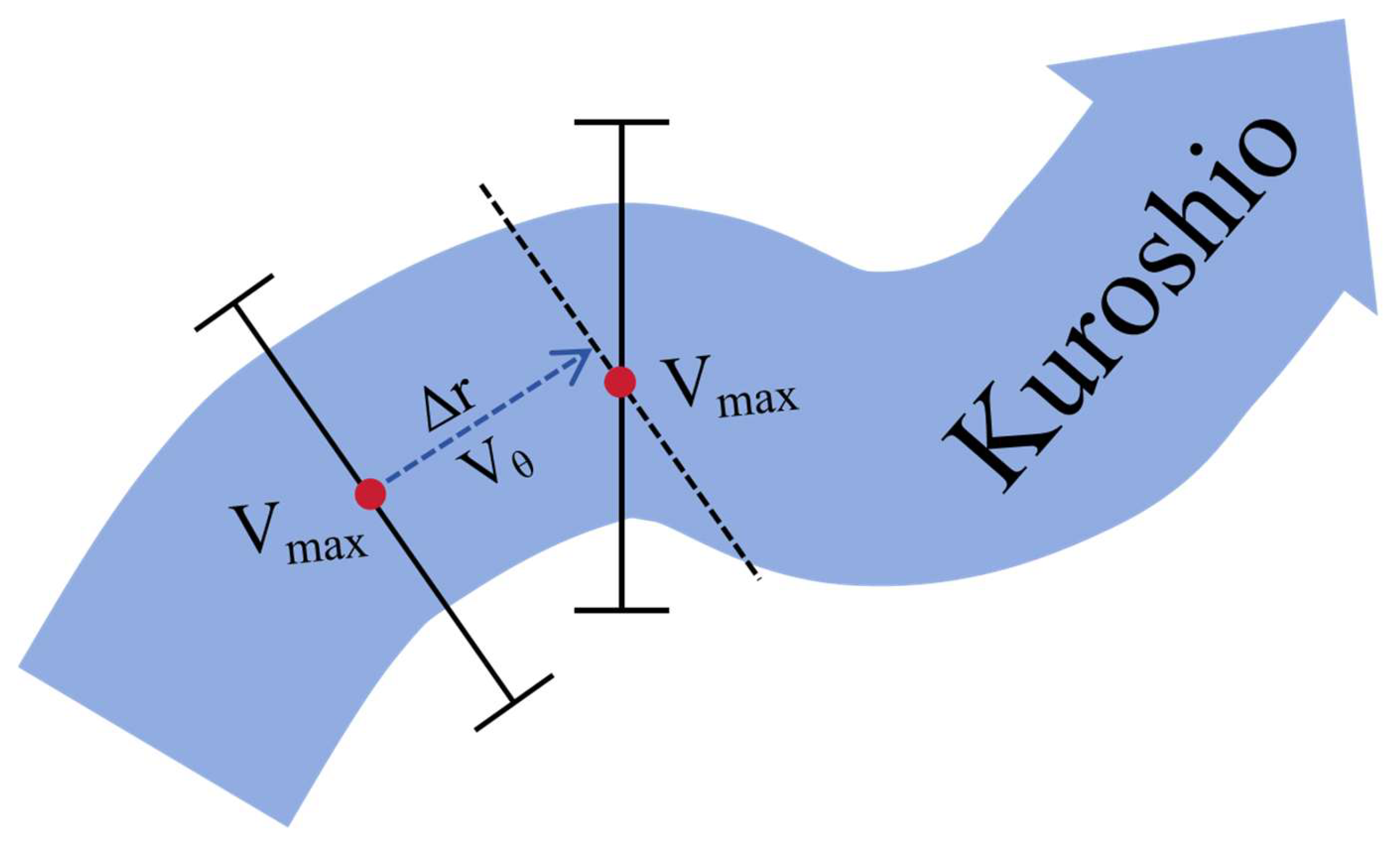
For simplicity, we assume that the cross-sectional velocity profile perpendicular to the flow direction is approximately unimodal with a single maximum (analogous to a Gaussian distribution), such that the point of maximum velocity corresponds to the main axis. However, in eddy-active or topographically complex regions, the velocity profile may deviate from a perfect Gaussian shape (e.g., bimodal or skewed). The proposed algorithm does not rely on the full Gaussian shape for fitting or uncertainty estimation; it only requires the location of the local maximum on the discretized search line. Therefore, the method remains applicable even when the profile is non-Gaussian, as the maximum remains the most physically relevant indicator of the current core. The Gaussian assumption is merely a conceptual justification and not a strict computational requirement. To this end, a line perpendicular to the flow direction is determined based on the flow direction at this point. The line is then divided into m discrete points, and bilinear interpolation is performed at each point to calculate the magnitude of the velocity. Among all valid points on the vertical line, the coordinates corresponding to the maximum velocity are determined; this point serves as the Kuroshio main axis node for the current iteration step (Figure 1).

3.1.3. Compared to Traditional Kuroshio Main Current Extraction Methods

Following the implementation of adaptive extraction of the Kuroshio main axis (the proposed algorithm, hereafter referred to as M1), this paper systematically and quantitatively evaluates the performance of four Kuroshio main axis extraction algorithms: M1 (the proposed dynamic vertical search), M2 (traditional maximum velocity tracking), M3 (velocity gradient ascent), and M4 (streamline integration).

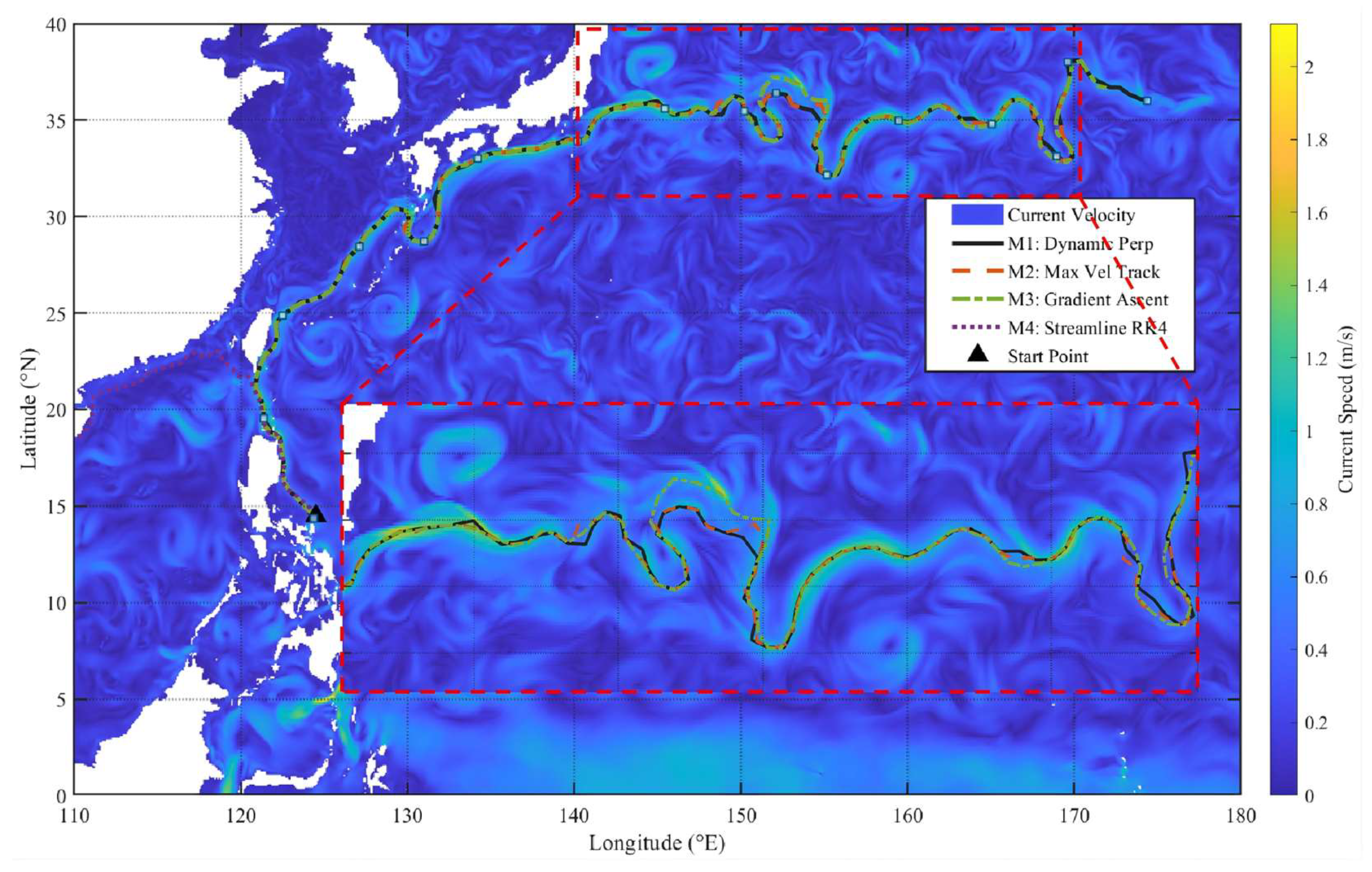
The spatial overlap of the trajectories (Figure 2) indicates significant differences among the algorithms when tracking mesoscale flow fields with pronounced meandering characteristics. The M1 and M2 algorithms were able to traverse the waters east of the Philippines to the Kuroshio Extension completely and clearly, successfully capturing the macroscopic curvature of the Kuroshio Main Channel and demonstrating exceptional global tracking capability. In contrast, the M3 algorithm, based on pure mathematical gradients, exhibited significant path distortion and deviation in the complex, vortex-dense region east of 140° E; meanwhile, the traditional streamline integration method M4 was captured by local vortex structures in the initial stage, completely losing its ability to track the main current axis over long distances.

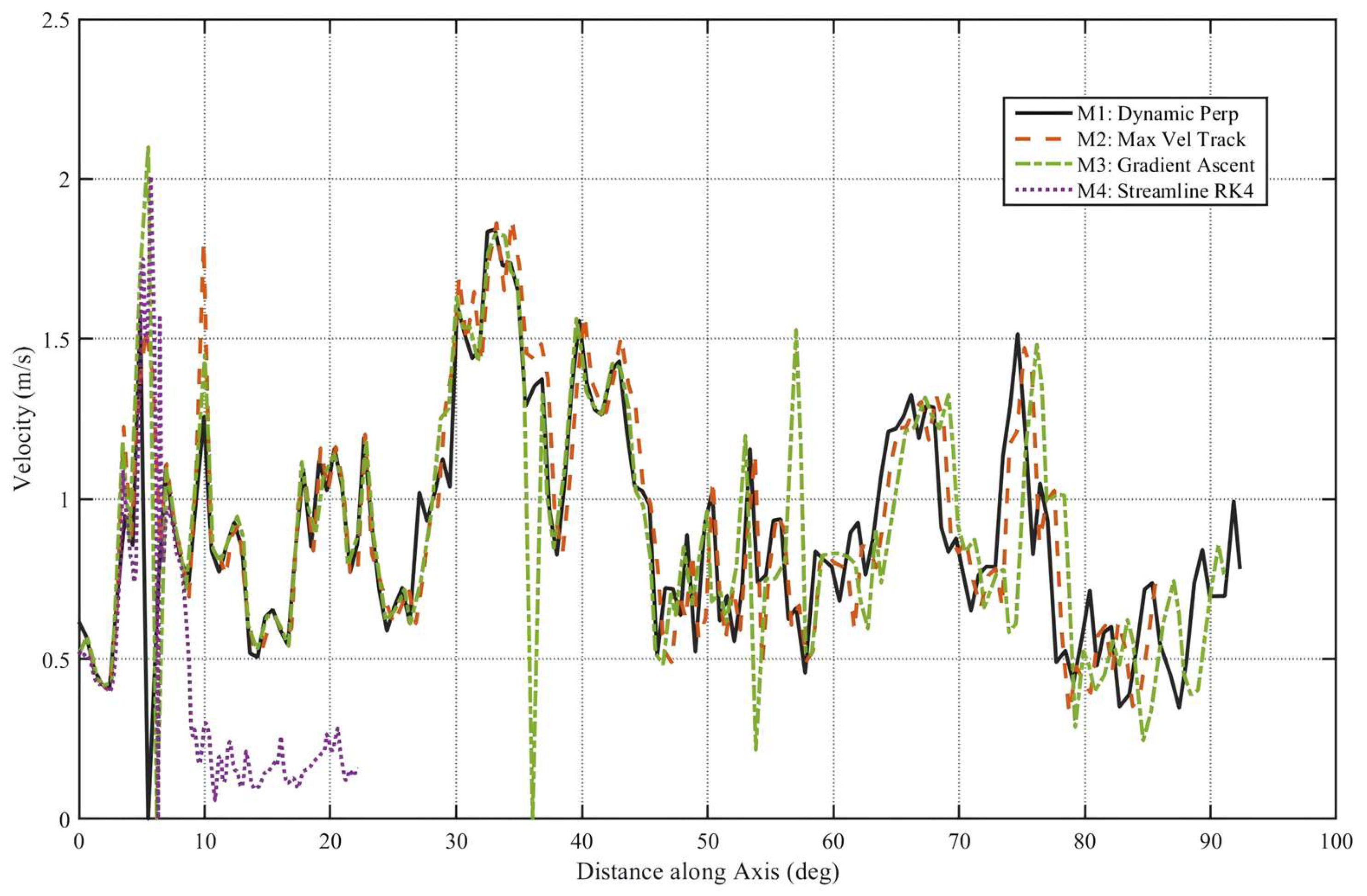
The velocity profiles along the main axis (Figure 3) further reveal the intrinsic characteristics of each algorithm at the level of physical mechanisms. Since the M2 algorithm directly targets local maximum velocities, the velocity values along its extracted path remain at peak levels in most sections, fully demonstrating its absolute ability to capture strong current cores. Although the velocity profiles of the M1 algorithm are occasionally slightly lower than those of M2, their overall variation is continuous and stable, effectively avoiding the violent oscillations in the path caused by an excessive pursuit of extrema, and better aligning with the physical reality of the continuity of the ocean current’s main axis. The velocity sequence of the M3 algorithm exhibits extreme anomalies, with sudden drops to near-zero at multiple nodes. This indicates that simple gradient methods are highly prone to becoming trapped in local stagnant zones or vortex centers within the velocity field, resulting in deviation from the main axis. Meanwhile, the premature deviation from the main axis in the M4 algorithm further confirms that the water particle trajectory tracking approach exhibits poor robustness when dealing with high-noise and closed streamline systems.

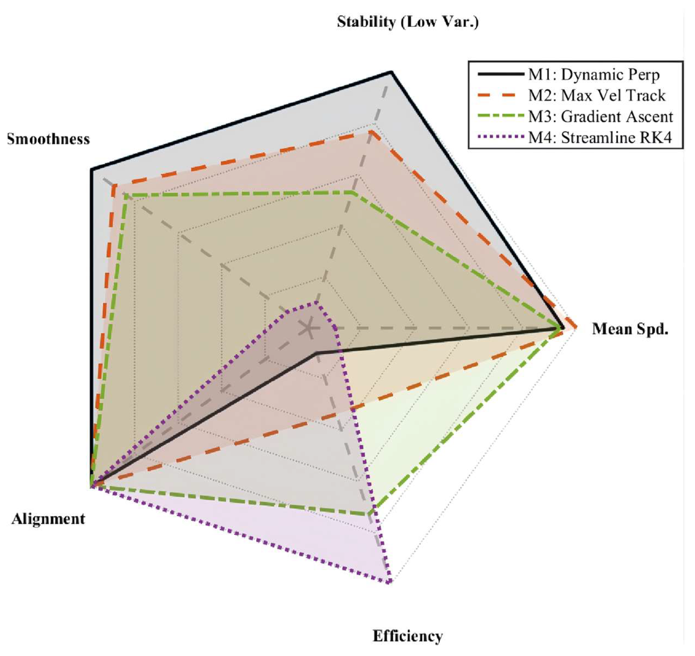
To further quantify the performance of different methods in main axis extraction, this paper has established five evaluation metrics: mean main axis flow velocity, flow velocity stability, smoothness, local peak alignment, and computational efficiency. Among these, the mean flow velocity along the main axis (Mean Spd.) is calculated by measuring the actual flow velocity at each point on the extracted main axis and then averaging the values across the entire axis. A higher value indicates that the extracted path more accurately captures the regions of strong flow; Velocity stability (Stability) is the statistical variance of the velocity at each point along the extracted main axis. Ideally, the main axis should extend along the core of the flow, with relatively stable velocity variations along its length. If the variance is too large, it indicates that the algorithm may be oscillating back and forth between the core and the edge regions; Smoothness is measured by calculating the average curvature of the path. Due to inertia and topographical constraints, the actual ocean current main axis is a relatively continuous and smooth curve. A higher average curvature indicates a more “winding” path. Local Peak Alignment is calculated as the ratio of each point on the main axis to the maximum flow velocity in that local region, measuring the degree to which the main axis deviates from the flow velocity ridge line. If the ratio is close to 1, it indicates that the method has accurately located the local peak flow velocity; if the ratio is low, it indicates that although the algorithm follows the flow direction, it has deviated toward the flanks of the main axis; Computational Efficiency evaluates the algorithm’s computational complexity. However, during the comparison, since these five metrics have completely different units (e.g., velocity is in m·s⁻¹, variance is a numerical value, and time is in seconds) and their evaluation criteria differ (some metrics are better when larger, while others are the opposite), To address this, this paper performed normalization to better compare the performance of each method, and the final results are shown in Figure 4.

A comprehensive, multi-dimensional quantitative evaluation model confirms that the M1 algorithm has significant advantages in terms of smoothness and alignment with local peaks. It can generate a continuous main axis that best matches the characteristics of ocean dynamics, making it the optimal choice that balances accuracy and physical significance. The M2 algorithm performs well in terms of average flow velocity and is more suitable for research scenarios highly sensitive to regions of extreme flow velocity. Although both algorithms incur significant computational costs, their high robustness in complex ocean environments fully compensates for this drawback. In contrast, while the M3 and M4 algorithms exhibit apparent high computational efficiency, they perform poorly on core physical metrics such as smoothness and alignment, and in some cases even fail to extract the main axis. It is evident that, in real oceanic settings with mesoscale vortices, extraction strategies relying solely on local mathematical features (such as streamlines or gradients) are difficult to apply. The introduction of dynamic spatial constraints (such as the normal search boundary in M1) is key to achieving high-precision extraction of the main axis of ocean currents.

3.1.4. Independent Validation Using SST Frontal Gradient

To substantiate the physical reliability of the extracted Kuroshio main axis beyond internal cross-comparisons among velocity-based methods, we conducted an independent validation against satellite-derived sea surface temperature (SST) data (OISSTv2, 2002–2024), a dataset entirely independent of the GLORYS12V1 velocity field. The underlying hypothesis is that the Kuroshio, as a warm western boundary current, generates a permanent thermal front against the adjacent cooler water. A physically plausible velocity-derived main axis should therefore be spatially collocated with the zone of maximum SST gradient.

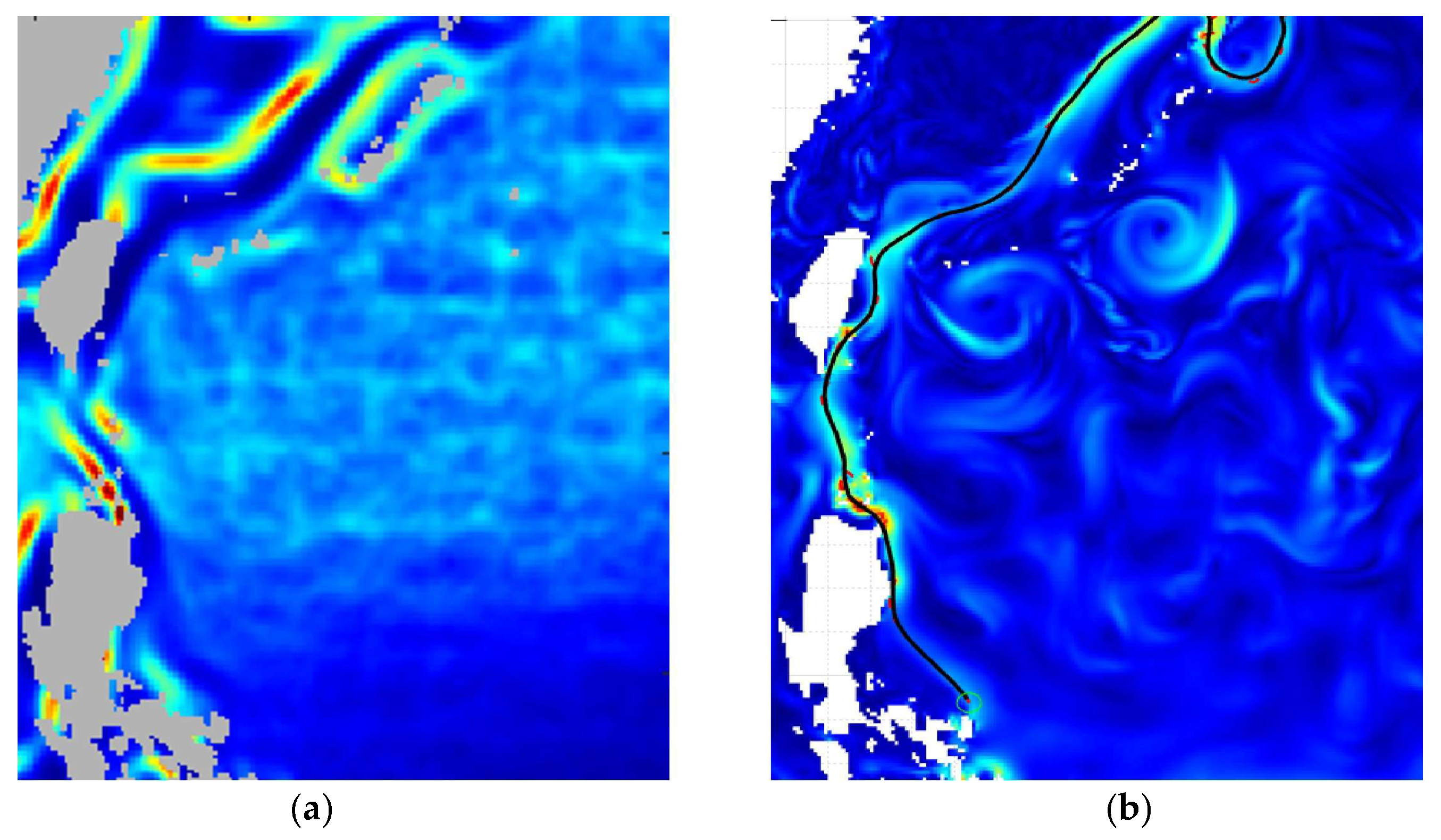
Figure 5 presents a representative snapshot (e.g., frequency of sea surface temperature gradients during the winter months from 2002 to 2024) showing the M1-derived Kuroshio main axis superimposed on the SST gradient field (magnitude of SST gradient computed via a Sobel operator). The close spatial correspondence is evident: the axis consistently tracks the maximum gradient band across the entire studied domain, from the NEC bifurcation zone to the Luzon Strait, despite no gradient information being used in the tracking process. Quantitative evaluation across the 2002–2024 period shows that the median Euclidean distance between the M1 axis and the SST gradient maximum is less than 0.2° (approximately 20 km), well within the typical width of the Kuroshio front.

This independent verification using an alternative physical field (SST) provides strong evidence that M1 does not merely optimize a velocity-specific metric but recovers a dynamically meaningful and physically consistent Kuroshio main axis. In contrast, the traditional M2 (maximum velocity tracking) and M3/M4 methods are shown to be more susceptible to local vorticity noise, frequently deviating from the SST gradient core in eddy-active regions.

3.2. Changes in the Characteristics of the Kuroshio Front and Discussion

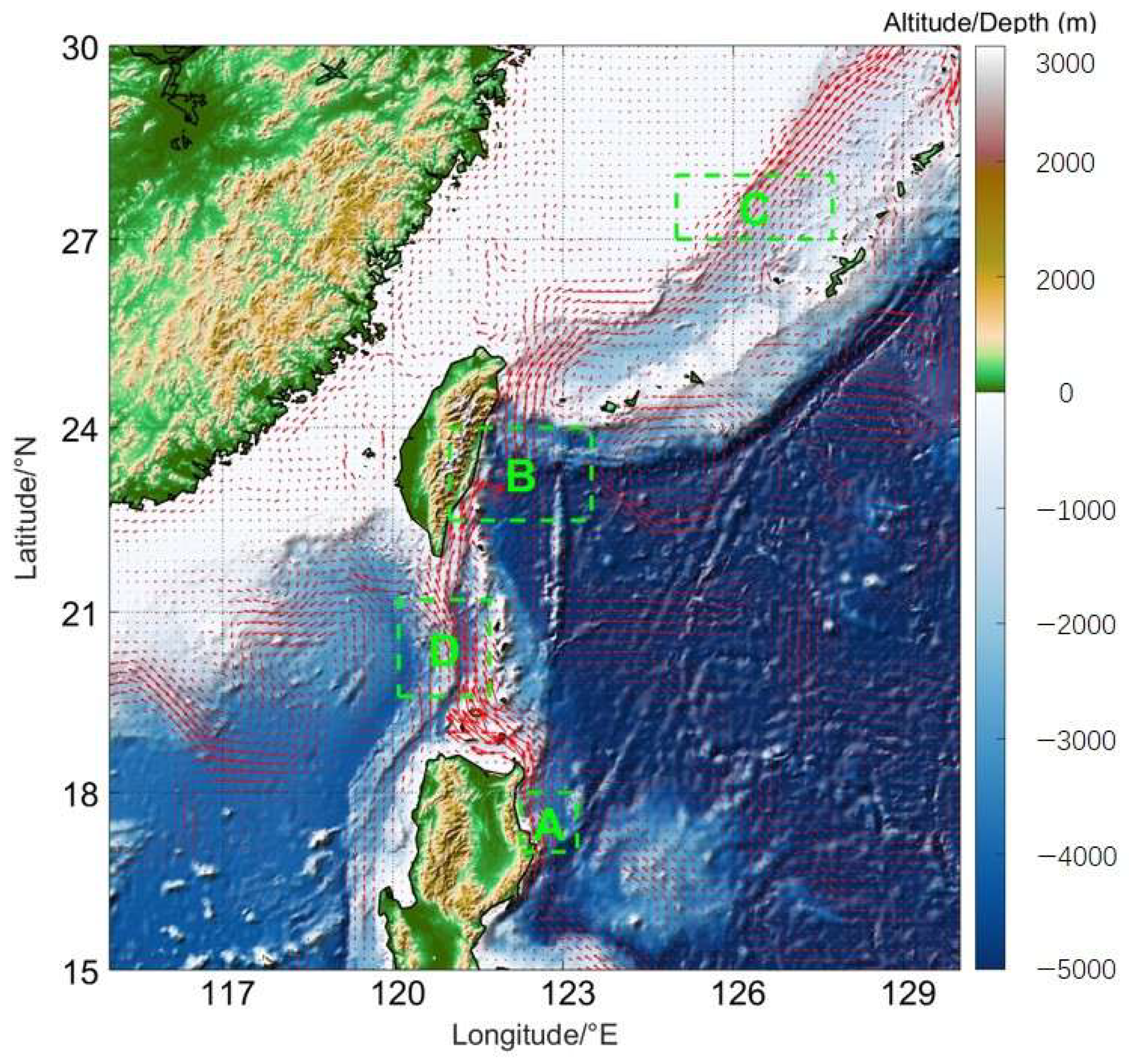
In our study of the Kuroshio Current, we selected four regions (Figure 6)—the Pacific NEC branching zone (A), the Kuroshio front east of Taiwan (B), the East China Sea Kuroshio front (C), and the Kuroshio intrusion zone in the Luzon Strait (D)—as representative areas of the Kuroshio Current. Spatially, these regions form a complete chain representing the Kuroshio’s generation at its source, main-channel transport, shelf interaction, and intrusion into marginal seas, covering several key stages of the Kuroshio’s multiscale variability.

3.2.1. The Branching Zone of the North Equatorial Current (NEC) in the North Pacific

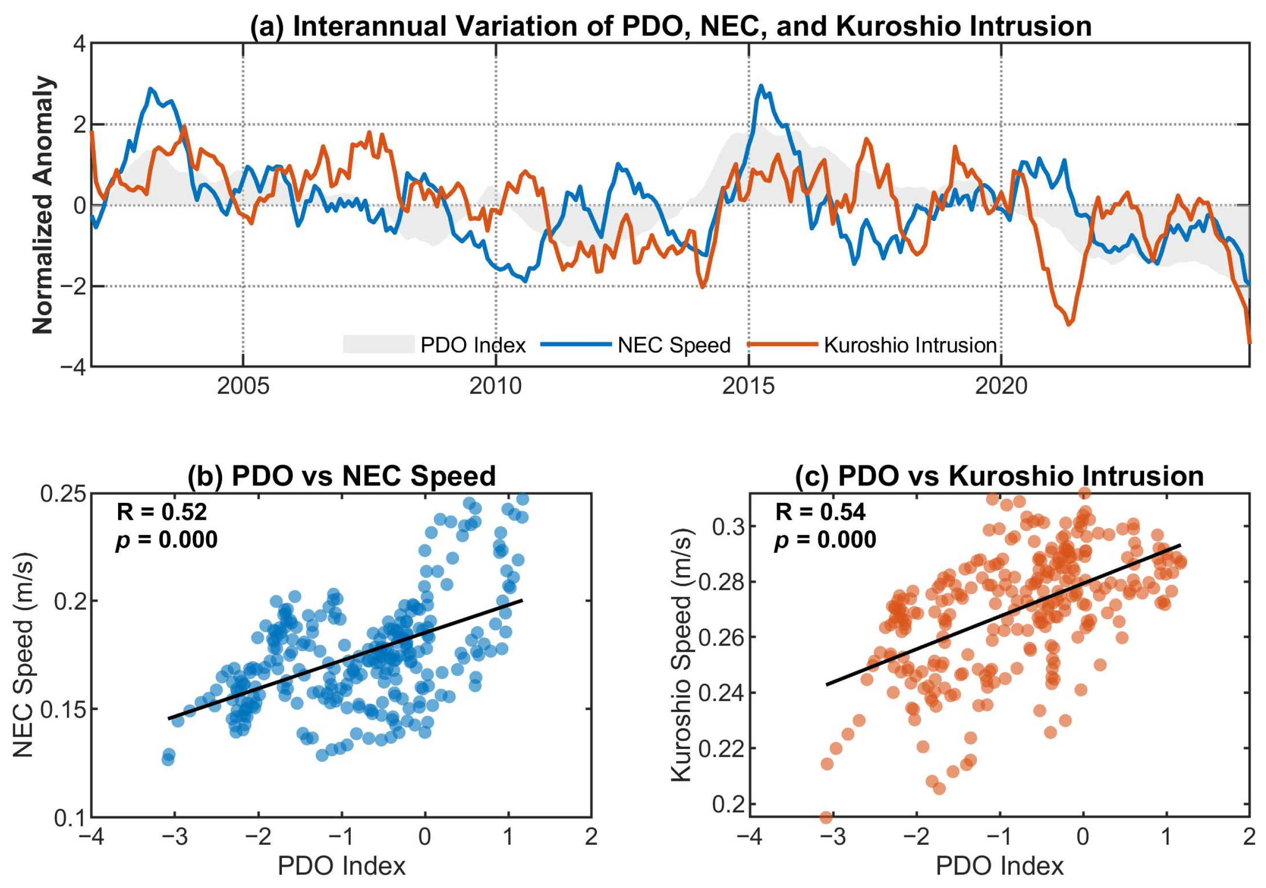
The North Equatorial Current (NEC) bifurcation zone in the North Pacific, as the key region where the Kuroshio originates, serves as the juncture where the NEC gives rise to the Kuroshio and the Mindanao Current. It directly determines the Kuroshio’s initial flow rate, water mass properties, and initial path, among other characteristics. It is also a critical area for the interaction between the tropical and subtropical Pacific circulations, and its variability is influenced by the Pacific Decadal Oscillation (PDO), the El Niño-Southern Oscillation (ENSO) [11,12], and serves as the upstream driver of variability in downstream Kuroshio segments. Selecting this region allows for an analysis of the fundamental mechanisms underlying Kuroshio front variability at its source [13,14,15].

As shown in Figure 7, the total flow velocity in the North Equatorial Current (NEC) bifurcation zone (black curve) during 2002–2024 generally ranged between 0.1 and 0.3 m·s⁻¹, with a peak approaching 0.4 m·s⁻¹. The low-frequency component (red curve, extracted by the 60-month low-pass filter) exhibits a broad fluctuation on timescales of approximately 10–15 years, with a continuous decline from 2002 to 2006, a gradual recovery from 2006 to 2014, followed by a significant decline to a trough of approximately 0.12 m·s⁻¹ from 2014 to 2018, and a subsequent strengthening after 2018. Given the limited data length (2002–2024), this fluctuation should be interpreted as low-frequency variability rather than a strictly periodic decadal cycle. This evolution is coupled with the synergistic effects of the Pacific Decadal Oscillation (PDO) and the El Niño-Southern Oscillation (ENSO) [16], with the strong El Niño event of 2014–2016 directly leading to an abnormal weakening of the NEC. The seasonal component (blue curve) exhibits a regular annual oscillation with an amplitude of approximately 0.07 m·s⁻¹; its seasonal-scale variability is driven by monsoon circulation: during winter (December–February), the northeast monsoon prevails, and the NEC significantly intensifies; in summer (June–August), the southwest monsoon dominates, and the NEC weakens markedly or even reverses its flow direction. The interannual anomaly component (green curve) exhibits a 2–7-year oscillation period, with significant extremes occurring in 2014–2016 and 2020–2023, corresponding to flow anomalies induced by strong El Niño and La Niña events through the modulation of the longitudinal displacement of the NEC bifurcation point. The residual component (gray curve, period < 6 months) has an amplitude of 0–0.2 m·s⁻¹ and is primarily composed of mesoscale vortices, tidal perturbations, and observational noise, constituting another major factor in flow velocity variability in this region.

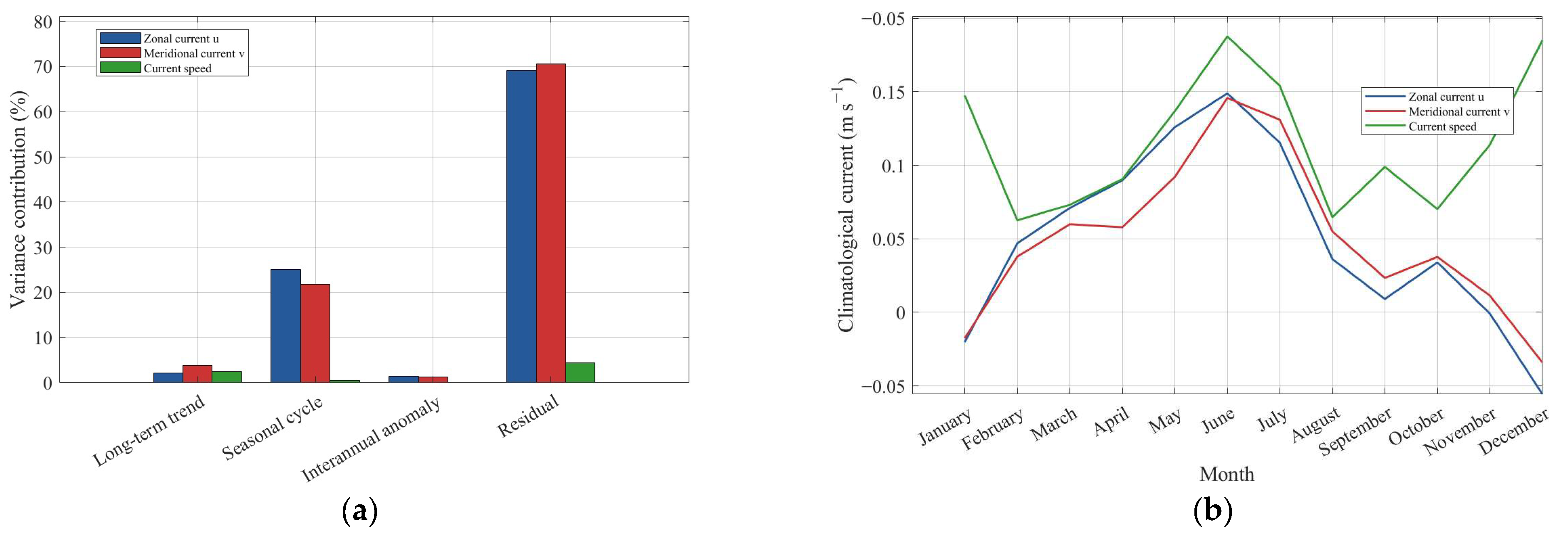
Variance contribution analysis (Figure 8) quantifies the relative contributions of components at different time scales to the variability of the zonal flow, meridional flow, and velocity modulus. The results show that the variability of the zonal flow is dominated by seasonal cycles, accounting for 29% of the variance. This is consistent with the nature of the North Equatorial Current (NEC) as a typical wind-driven current, whose seasonal-scale variability is directly caused by the periodic changes in the trade winds [17]. In contrast, the variability of the meridional flow is most significantly influenced by long-term, low-frequency trends (15%), which intuitively reflects the decadal oscillations in the meridional position of the NEC bifurcation point. A composite analysis of the monthly average flow velocities over multiple years in this region clearly reveals the seasonal characteristics of the ocean current system: the zonal flow exhibits a westward negative component (approximately −0.05 m·s⁻¹) from January to April, then shifts to a positive eastward direction from May to December, peaking in July (0.08 m·s⁻¹). This confirms that the NEC exhibits a significant seasonal reversal in flow direction: in winter, it is modulated by the northeastern monsoon, resulting in a strong westward flow, while in summer, under the influence of the southwestern monsoon, an eastward return flow occurs or the flow velocity significantly weakens. The meridional flow approaches zero in January, increases rapidly northward from February to May, and peaks in April (0.045 m·s⁻¹). It then shifts southward, reaching a minimum in August (−0.045 m·s⁻¹), before rising northward again in October. This pattern aligns with the seasonal oscillation of the NEC branching point, which shifts northward in spring and southward in autumn. The current velocity remained within the range of 0.05–0.085 m·s⁻¹ throughout the year, peaking from July to September (0.085 m·s⁻¹), corresponding to the characteristic of active but variable flow directions in the summer current system; the second-highest velocity was observed from January to February (0.055 m·s⁻¹), reflecting the stable structure and strong dynamics of the winter current system. The study area is located in the transition zone between the tropical and subtropical regions, where ocean current variations are jointly regulated by the transition between the monsoon and trade winds: during the summer (May–September), the southwest monsoon prevails, not only weakening but even reversing the direction of the NEC, while simultaneously intensifying the local Ekman suction effect; in winter, the northeast monsoon significantly enhances the strength of the westward branch of the NEC, collectively leading to the seasonal variations in ocean currents in this region [17].

The results of the Mann–Kendall trend test in Figure 9 reveal the long-term statistical evolution of ocean currents in the North Equatorial Current (NEC) bifurcation zone. From 2002 to 2024, both zonal and meridional flow velocities showed an increasing trend (p < 0.01), indicating that the overall flow in this region has been steadily intensifying. In contrast, the long-term changes in current magnitude did not reach statistical significance (p = 0.0678), suggesting that the amplitude of current velocity did not follow a definite linear trend during the study period; the long-term variability of the flow field was primarily manifested as systematic adjustments in flow direction. These characteristics are presumed to be closely related to large-scale circulation adjustments, such as the strengthening of the Walker circulation in the tropical Pacific [18] and the intensification of trade winds [19], against the backdrop of global warming [20]. The strengthening of the Walker circulation leads to an increase in the east–west sea surface gradient in the equatorial Pacific, while the intensification of the trade winds further drives the westward transport of the North Equatorial Current. At the same time, by regulating the meridional displacement of the bifurcation point of the North Equatorial Current, both the zonal and meridional velocity components in this region exhibit a long-term increasing trend, whereas the continuous adjustment of the direction of the velocity vector does not show a significant linear change.

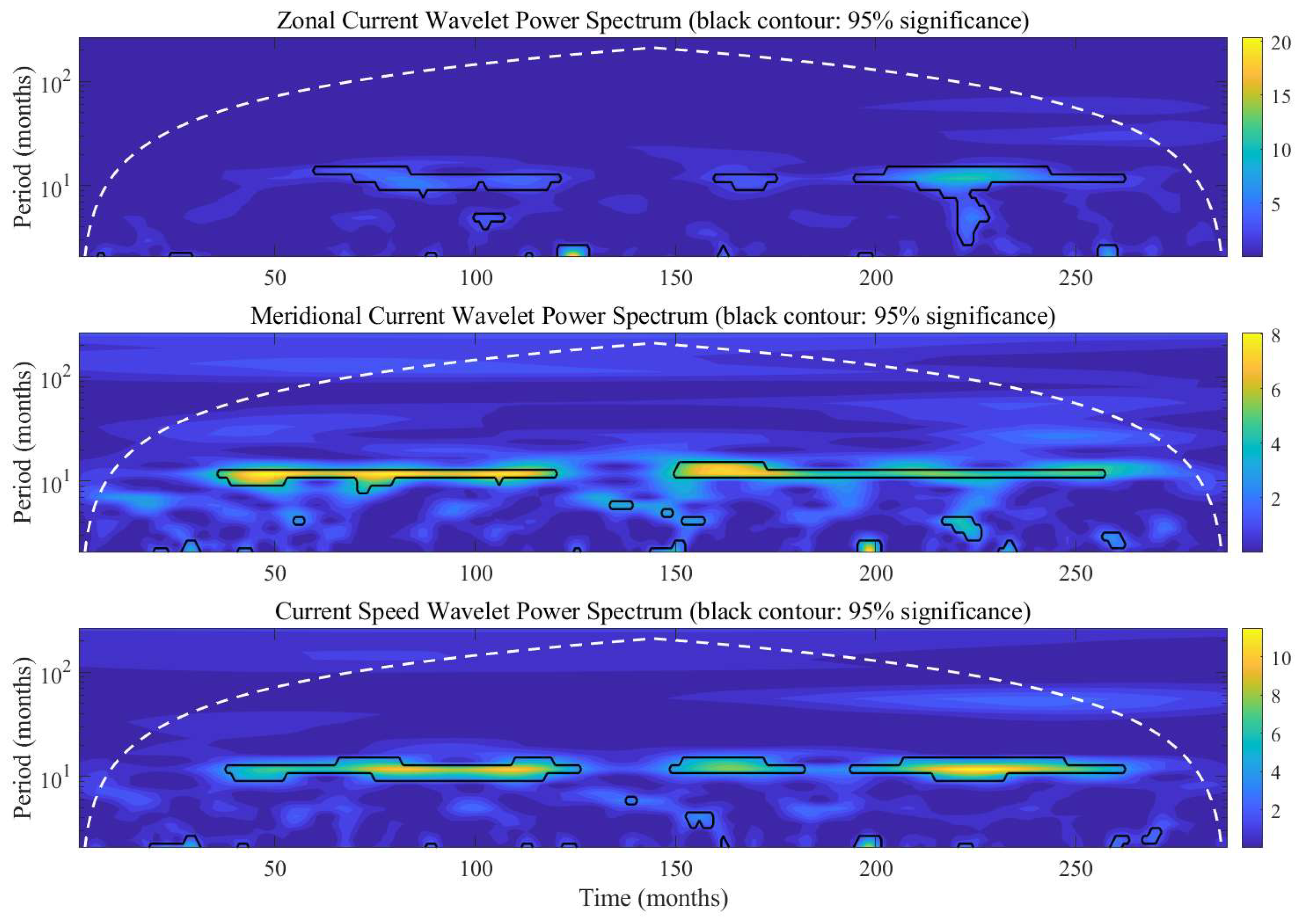
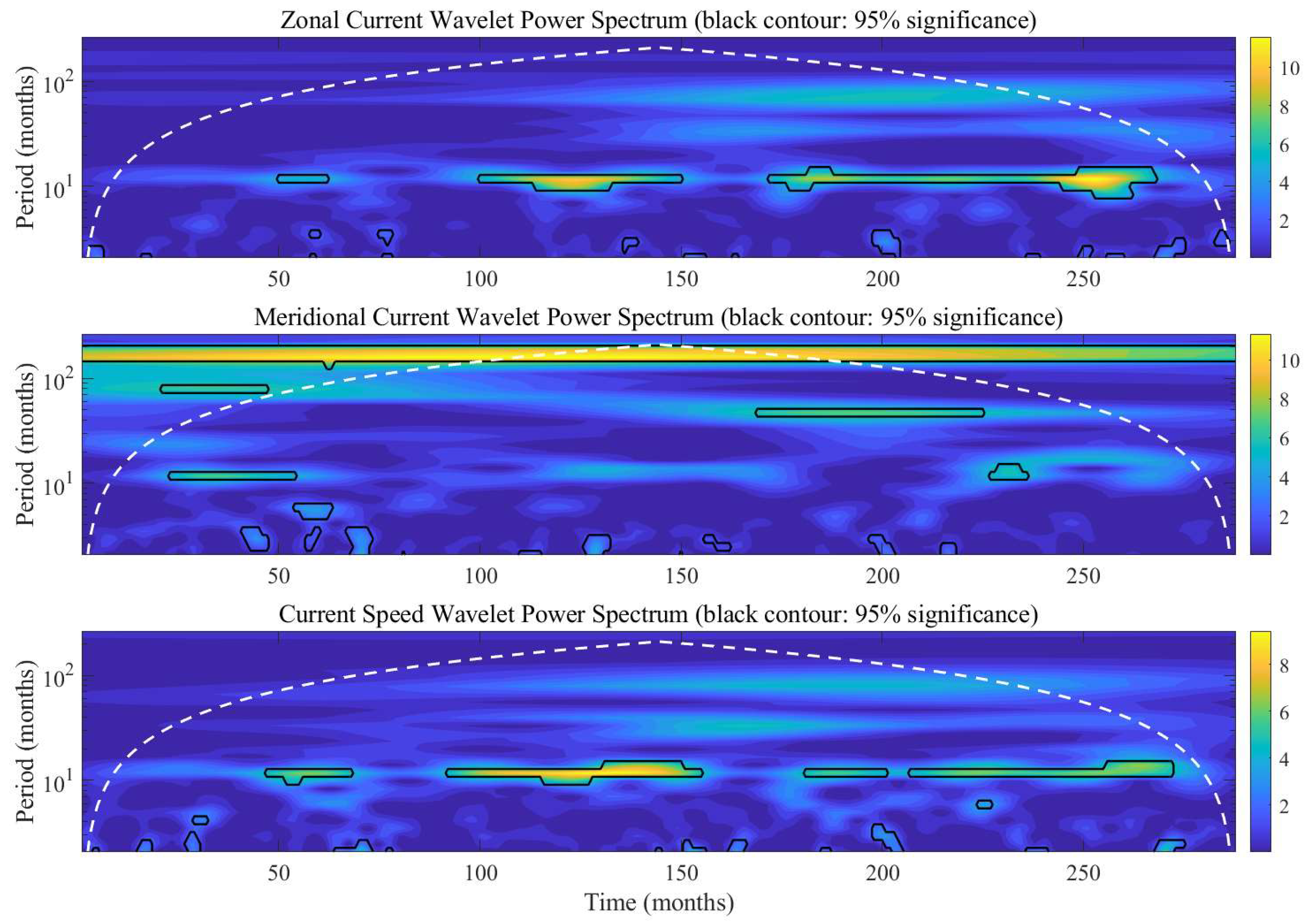
The results of the wavelet time-frequency analysis in Figure 10 illustrate the time-frequency distribution characteristics of the flow field energy during the study period. For the zonal velocity component, spectral energy is concentrated at a significant 12-month periodic scale (i.e., the seasonal scale). This signal exhibits a sustained increase in energy during the periods 2002–2005, 2010–2014, and 2020–2024, reaching a spectral peak after 2020, indicating that the seasonal signal possesses high stability and persistence. Further analysis reveals that the amplitude of the seasonal-scale signal exhibits a significant response to modulation by El Niño-Southern Oscillation (ENSO) events [21]. For example, following the strong El Niño event of 2015–2016, the energy of this seasonal signal was further amplified, revealing the key regulatory role of large-scale tropical climate modes in the seasonal variability of local circulation in the NEC branching region. In contrast, the energy distribution of the meridional velocity component exhibits different characteristics, with notable wavelet power appearing at timescales exceeding 100 months. However, this power does not pass the 95% significance test against red noise, indicating that no stable decadal period can be robustly identified under the current data length. The low-frequency variability of the meridional flow is therefore interpreted as a non-stationary, multi-year to decadal fluctuation. This signal persists throughout the entire study period with stable energy, constituting the background for variations in the meridional velocity component; simultaneously, a 12-month seasonal-scale signal is superimposed on the spectral structure of the meridional component, reflecting the combined driving and superposition effects of the interdecadal background field and intraseasonal variability on the meridional flow [22].

3.2.2. Changes in the Characteristics of the Kuroshio Front East of Taiwan

The Kuroshio Front east of the Gulf of Taiwan is the initial segment of the main Kuroshio Current as it enters the waters off the Chinese coast in the northwestern Pacific, linking the Kuroshio source region with the East China Sea shelf system. Among its characteristics, the oscillation of the Kuroshio main axis [23], baroclinic nature of the front [24], and dynamic stability are most pronounced. Simultaneously, it is jointly regulated by the East Asian monsoon, mesoscale vortex activity, and interannual climate anomalies [25]. As a representative segment for the multiscale variability patterns of the Kuroshio main axis frontal zone, selecting this region effectively illustrates the dynamic variability characteristics of the Kuroshio main branch and provides a reference for analyzing the variability mechanisms in downstream areas.

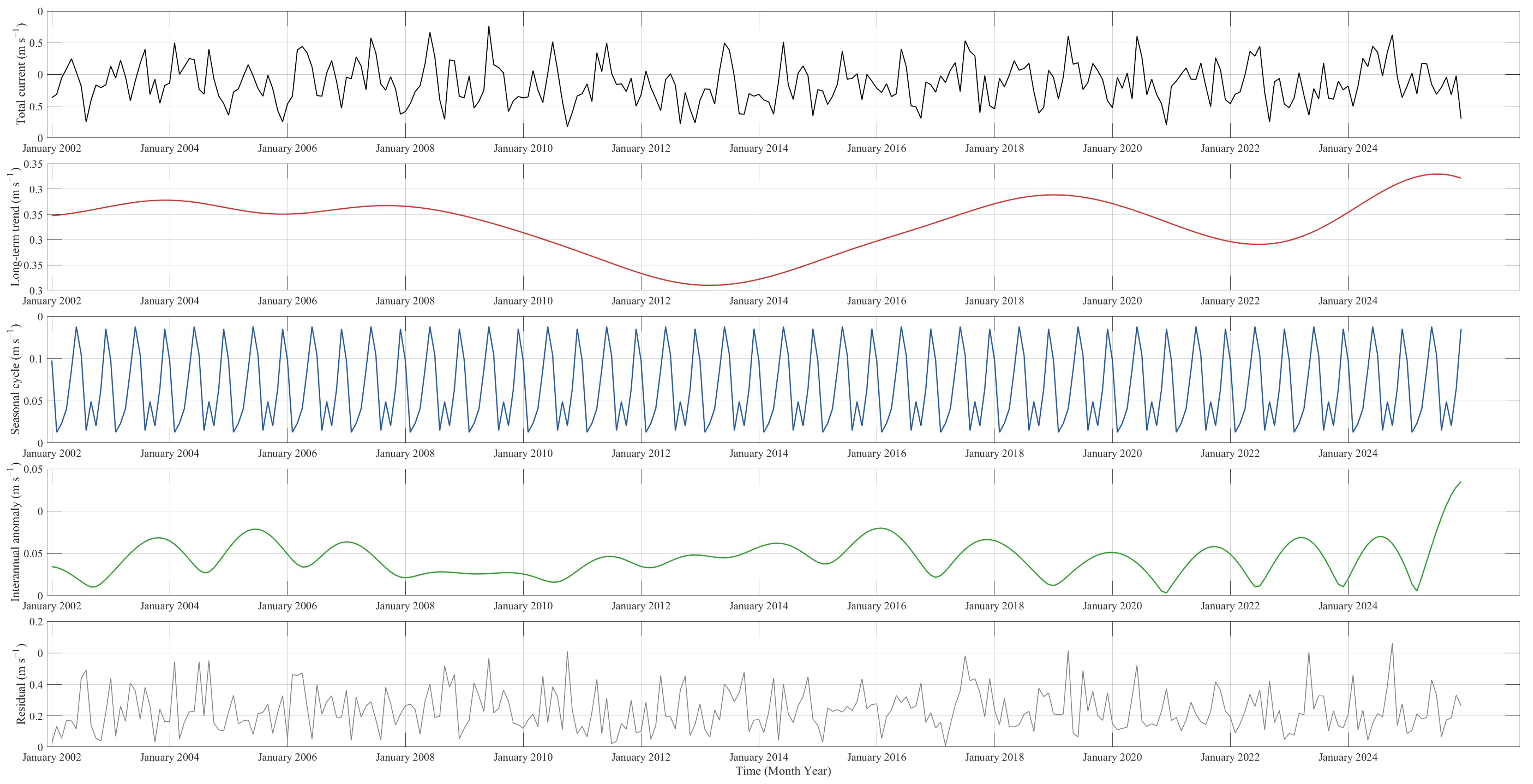
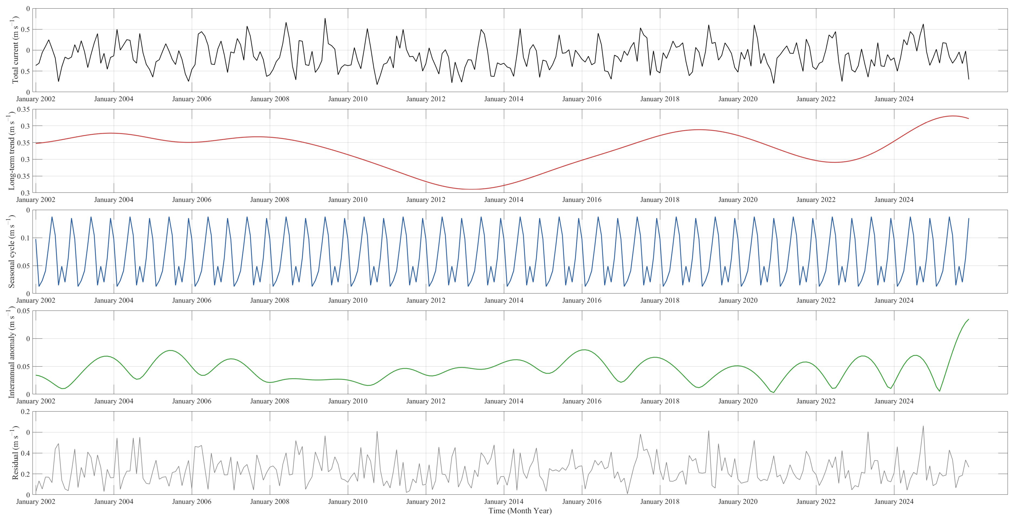
As shown in Figure 11, the average current velocity in the Kuroshio region east of Taiwan ranges between 0.2 and 0.6 m·s⁻¹, with the time series exhibiting characteristics of superimposed periodic fluctuations and high-frequency irregular oscillations. The long-term low-frequency component exhibits a clear decadal oscillation pattern: it showed a gradual decline from 2002 to 2013, reaching a trough (approximately 0.31 m·s⁻¹) in 2013; it continued to rise from 2013 to 2019, reaching a phase peak (approximately 0.35 m·s⁻¹) in 2019; from 2019 to 2022, it declined slightly, but began to strengthen significantly again starting in 2022, reaching its highest value for the entire period (approximately 0.37 m·s⁻¹) around 2024. These decadal oscillation characteristics are closely related to the North Pacific Decadal Oscillation (PDO) and the multi-year-scale adjustment processes of the subtropical circulation [26,27,28]. The period from 2002 to 2013 corresponded to the cold phase of the PDO, during which the subtropical circulation weakened and the main axis of the Kuroshio Current shifted offshore, leading to a continuous decline in the Kuroshio current velocity east of Taiwan; After 2013 and 2014, the PDO shifted to a warm phase, the subtropical circulation strengthened, and wind-driven gyro-corrugation anomalies drove an increase in Kuroshio transport, causing the current velocity to rise accordingly; fluctuations after 2019 reflect the synergistic modulation between the PDO and local mesoscale eddy activity. This evolutionary pattern reveals the direct regulatory role of multi-year-scale adjustments in the subtropical circulation on changes in the main Kuroshio current velocity. The seasonal component exhibits a stable annual oscillation, with amplitudes ranging from 0 to 0.12 m·s⁻¹. The fluctuation patterns were highly consistent across all years from 2002 to 2024, representing the most stable deterministic signal in the current variability of this region and reflecting the seasonal adjustment patterns of the Kuroshio driven by the East Asian monsoon [29]. “The amplitude of the interannual anomaly component was generally confined to within 0.04 m·s⁻¹ during 2002–2020. After 2020, the amplitude showed larger values, reaching approximately 0.06 m·s⁻¹ around 2024. This indicates an enhancement of interannual variability (i.e., larger year-to-year fluctuations) in recent years, rather than a statistically significant long-term linear trend (see M-K test results in Figure 12, p > 0.05).” [30].

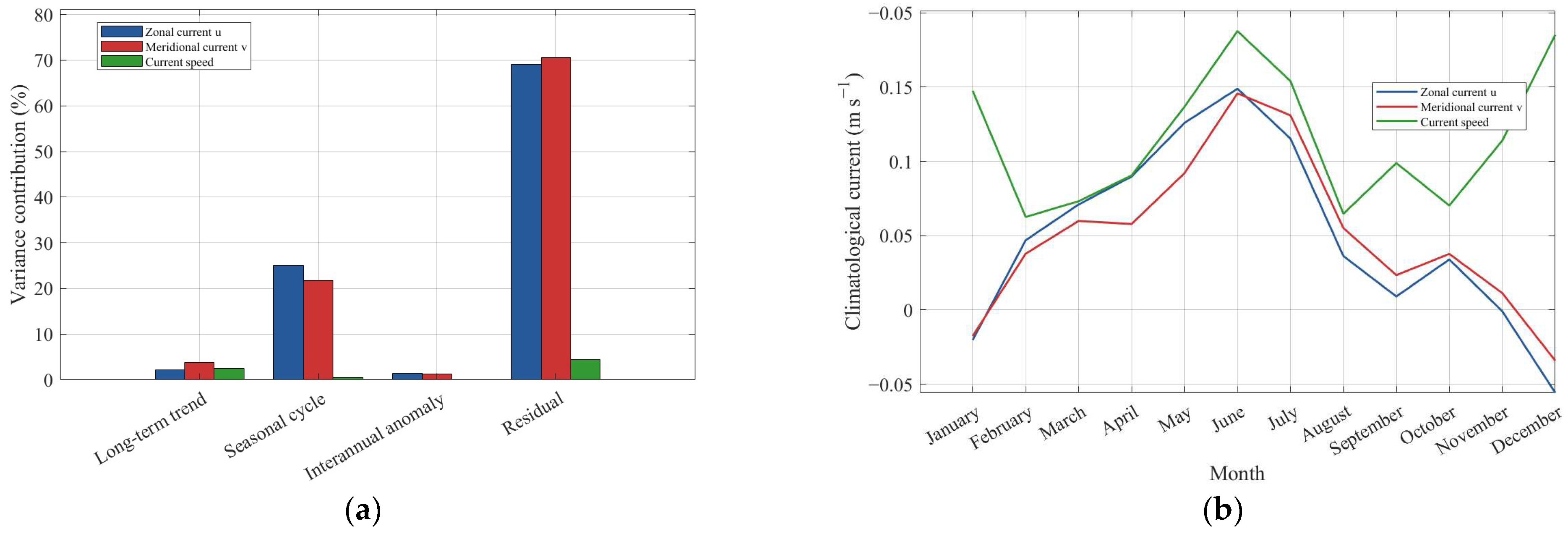
The results of variance decomposition (Figure 12) indicate that the variability in the zonal (u) and meridional (v) velocity components of the Kuroshio Current east of Taiwan exhibits highly consistent energy distribution characteristics, with high-frequency residual terms accounting for approximately 70% of the variance, indicating that mesoscale and subseasonal processes play a primary role (see Section 2.4 for a discussion of potential methodological biases) [31,32]; Seasonal cycles are the secondary contributors, explaining approximately 25% of the total variability in the u-component and 22% in the v-component, respectively, while the variance contributions from long-term low-frequency variability and interannual anomalies are both less than 5%. These results indicate that the variability of the Kuroshio current velocity vectors in this region is primarily co-regulated by high-frequency dynamic processes such as mesoscale vortices and the seasonal cycle driven by the East Asian monsoon, while the contributions of multi-year trends and interannual anomalies are relatively weak [33]. In contrast, the distribution of energy in the variation in current magnitude shows significant differences, with variance primarily originating from long-term low-frequency variability (approximately 3%) and high-frequency residual terms (approximately 5%), while the contributions of seasonal cycles and interannual anomalies are nearly negligible. This is primarily because the seasonal circulation of the Kuroshio east of Taiwan is mainly manifested as seasonal oscillations of the flow axis, characterized by adjustments in the phase and direction of the u and v components, rather than seasonal increases or decreases in flow intensity. The main axis of the Kuroshio shifts eastward in summer and westward in winter, leading to significant seasonal shifts in the direction of the flow vector within the study area, which makes the contribution of seasonal variance in the u and v components prominent; Meanwhile, the magnitude of the velocity vector remains at a relatively high level in both winter and summer, with only a slight decline during the transitional seasons of spring and autumn. Consequently, the contribution of seasonal circulation to the total variation in velocity magnitude is extremely low [33], a characteristic consistent with existing observational results from the main Kuroshio current region.

Based on multi-year average seasonal circulation sequences, the zonal velocity u exhibits a superimposed annual and semi-annual cycle [34], reaching a westward trough in January (approximately −0.07 m·s⁻¹), an eastward peak in June (approximately 0.10 m·s⁻¹), and declining to a westward component in December (approximately −0.05 m·s⁻¹). This variation closely corresponds to the seasonal reversal of the East Asian winter and summer monsoons and the east–west oscillation of the Kuroshio main current. The meridional flow velocity v exhibits an annual cycle, with the northward component reaching a trough in February (approximately −0.01 m·s⁻¹), reaching a northward peak in June (approximately 0.095 m·s⁻¹), shifting to a southward direction in August, and reaching a southward peak in December (approximately −0.08 m·s⁻¹). This pattern aligns with the seasonal adjustments of the North Pacific subtropical circulation: in summer, the subtropical high shifts northward, strengthening northward transport by the Kuroshio; in winter, the subtropical high retreats southward, correspondingly weakening northward transport [35]. The magnitude of the flow velocity exhibits a distinct semi-annual biphasic structure, peaking in June and December (approximately 0.135 m·s⁻¹) and reaching troughs in February and August (approximately 0.01–0.015 m·s⁻¹) [36]. This characteristic results from the superposition of the seasonal phases of the u and v components. In June, both u and v are positive, and the vector sum reaches a maximum; in December, both u and v are negative, and the vector magnitude also rises to a peak. This creates a semi-annual pattern with higher flow velocities in winter and summer and lower velocities in the transitional seasons of spring and autumn. This variation is consistent with the dynamic processes of the seasonal oscillation of the Kuroshio’s main axis [37].

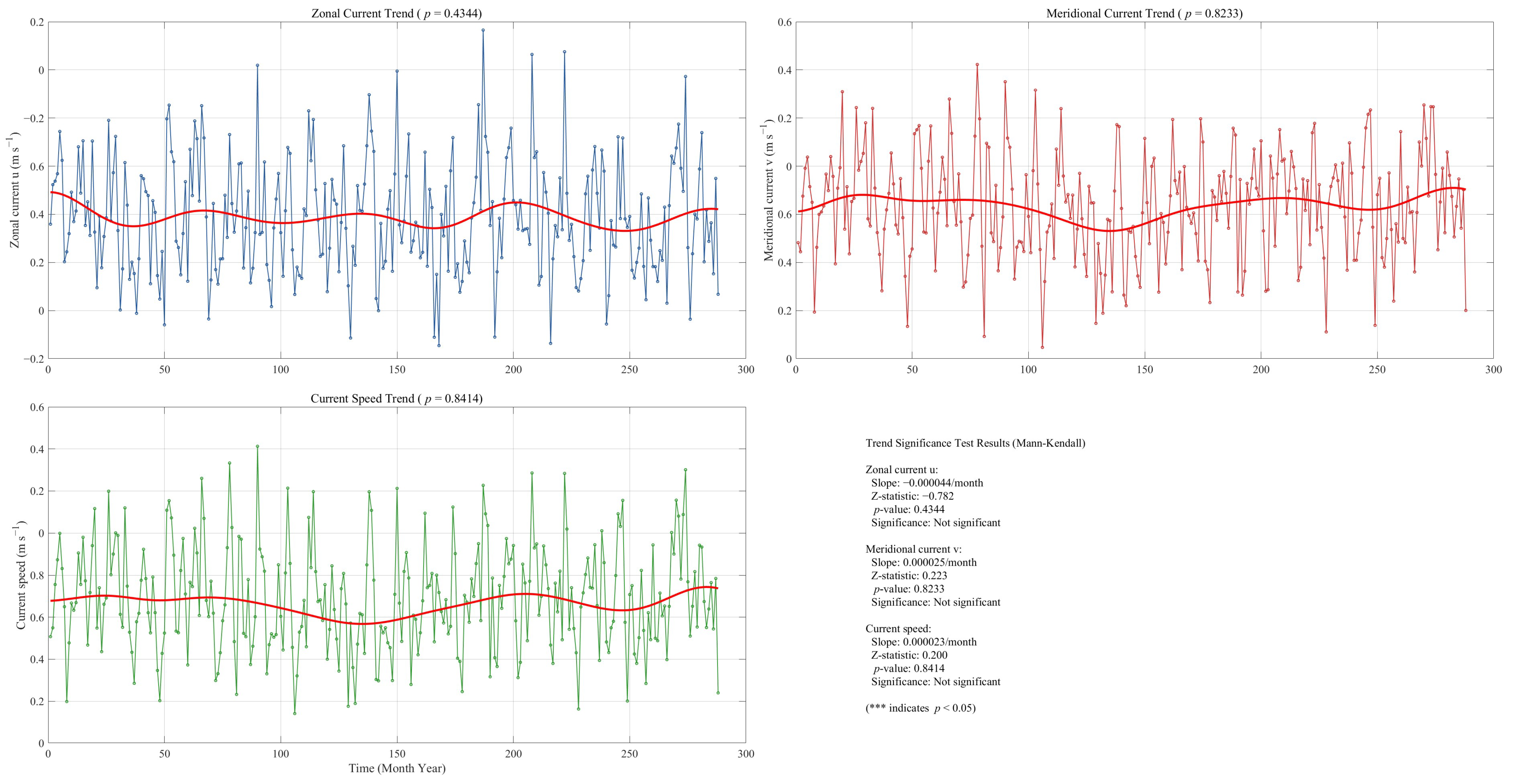
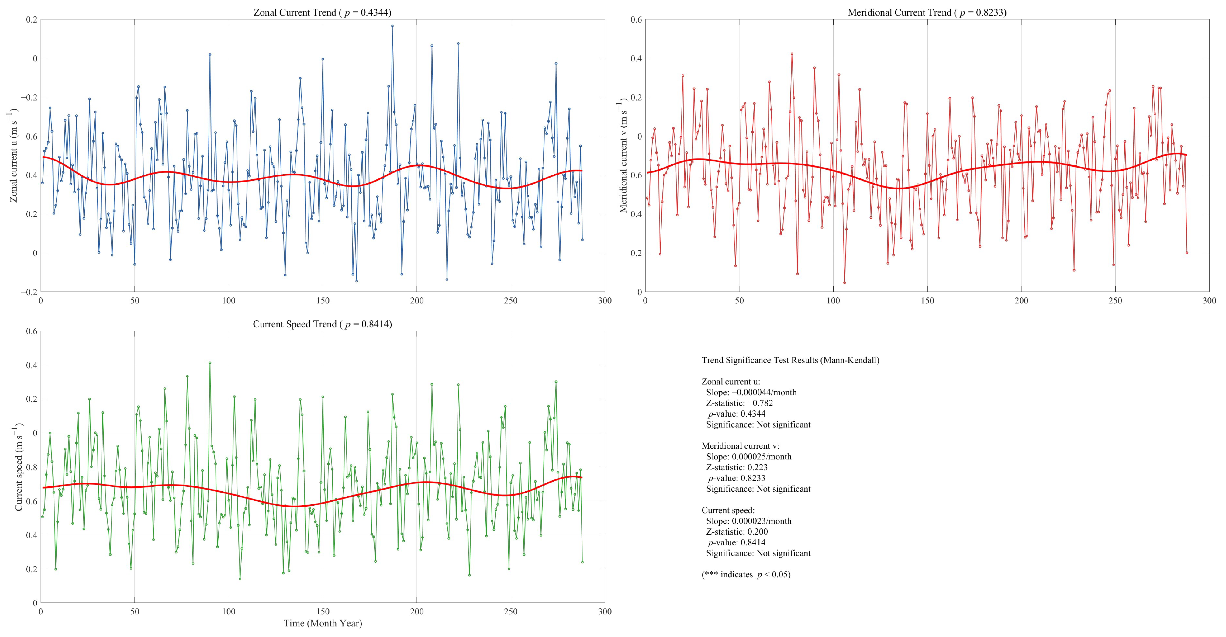
The results of the Mann–Kendall trend test (Figure 13) show that the zonal velocity u, meridional velocity v, and total velocity of the Kuroshio in the study area do not exhibit statistically significant long-term linear trends. It should be clarified that the absence of a significant linear trend does not imply that the Kuroshio in this region lacks multi-year-scale variability; rather, its long-term changes are characterized by decadal oscillations driven by large-scale climatic modes such as the Pacific Decadal Oscillation (PDO), rather than exhibiting a monotonically linear increase or decrease [38]. These results are consistent with the oscillatory characteristics revealed by the low-frequency variability components in this study, and are also in line with the findings regarding the long-term variability patterns of the Kuroshio [39,40].

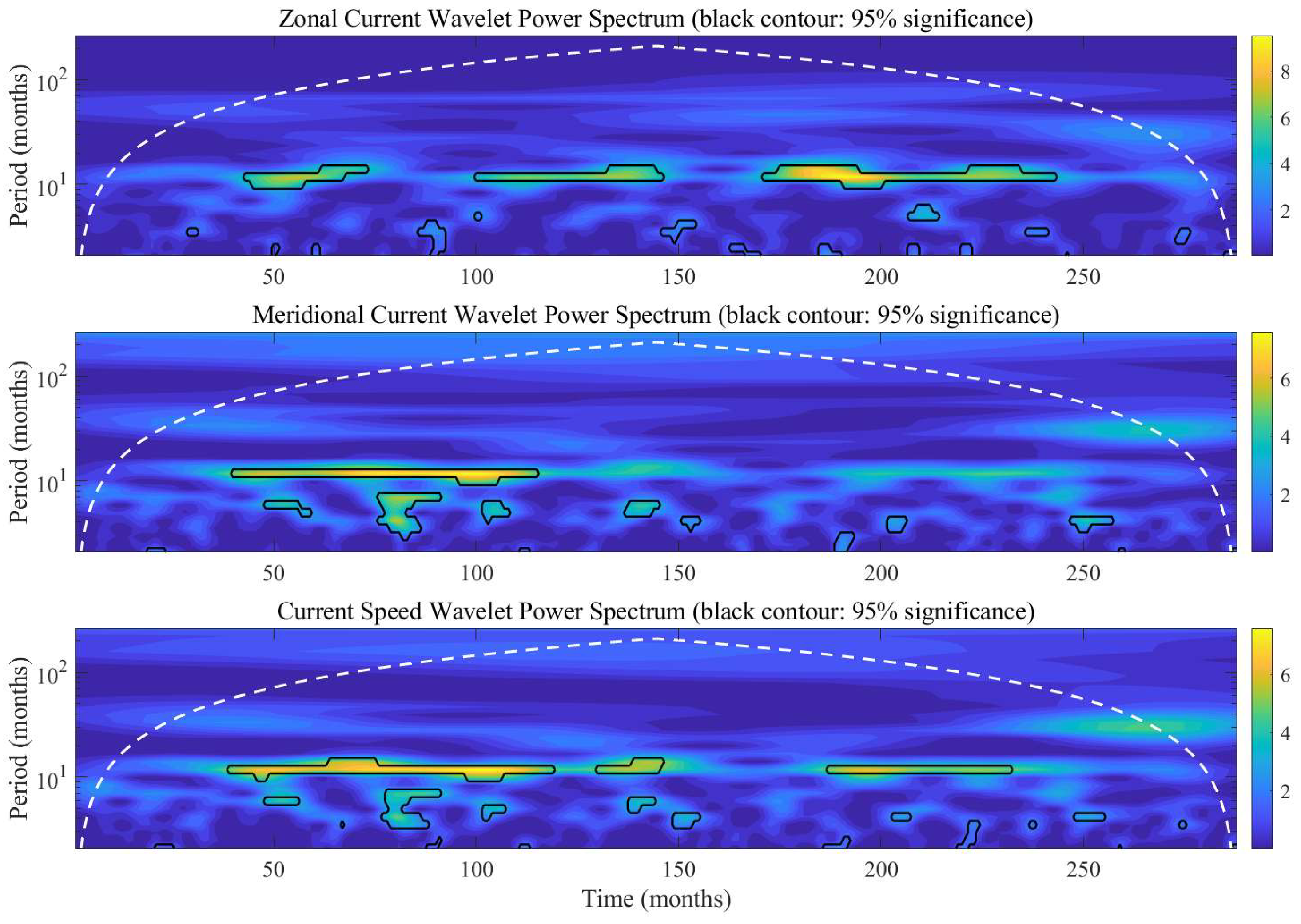
The results of the Morlet wavelet power spectrum analysis (Figure 14) indicate that, during the study period from 2002 to 2024, the Kuroshio’s zonal velocity u, meridional velocity v, and velocity magnitude in this region all exhibited a significant 12-month annual cycle signal throughout the entire time series, and all passed the significance test at the 95% confidence level; Among these, the annual cycle signal of the zonal velocity u exhibits the strongest energy and the most continuous temporal distribution, fully confirming that the seasonal cycle is the most stable and highest-energy periodic component regulating Kuroshio variability in this region; this conclusion is consistent with variance contribution analysis and the seasonal cycle characteristics of the climate state. At the same time, both the meridional velocity v and the velocity modulus exhibited significant 6-month semi-annual cycle signals. This signal is consistent with the semi-annual oscillation characteristics of the East Asian monsoon [41] and matches the bimodal seasonal evolution pattern observed in the velocity modulus, further confirming that the semi-annual cycle is a key component of the seasonal-scale variability of the Kuroshio in this region. Furthermore, none of the velocity components passed the 95% significance test at the interannual scale (24–84 months) or the decadal scale (100 months and above). This indicates that the Kuroshio in this region does not exhibit stable and significant periodic oscillatory characteristics at the interannual to decadal scales. This result is consistent with the conclusion from variance decomposition that the contributions of interannual anomalies and long-term trends are extremely low.

3.2.3. Changes in the Characteristics of the Kuroshio Front in the East China Sea

The Kuroshio Front in the East China Sea is the core region where the Kuroshio Current and the continental shelf system undergo strong dynamic coupling, driving the transport of energy, matter, and momentum from the Kuroshio Current to the continental slope of the East China Sea [42], It regulates the structure of shelf circulation, the evolution of frontal vortices, and the distribution of nearshore ecosystems and fishery resources [43]. This region is crucial for elucidating the dynamic adjustment mechanisms governing the transition of the Kuroshio from a strong western boundary current to a nearshore circulation, as well as for clarifying the direct regulatory effects of the Kuroshio on China’s nearshore environment. Selecting this area effectively highlights the characteristics of the Kuroshio’s interactions with the continental shelf.

As shown in Figure 15, the total Kuroshio current velocity in the study area from 2002 to 2024 remained stable between 0.2 and 0.6 m·s⁻¹. The temporal variation in current velocity exhibited significant quasi-periodic fluctuations overall, without showing any obvious long-term monotonically increasing or decreasing trends; the fluctuating energy was primarily concentrated at the seasonal and high-frequency weather scales [44,45]. The long-term low-frequency variability component did not exhibit a statistically significant linear trend but instead displayed a multi-phase interdecadal oscillation. From 2002 to 2006, the flow velocity continued to rise; from 2006 to 2012, it gradually declined to a trough (approximately 0.315 m·s⁻¹); from 2012 to 2018, it exhibited a fluctuating recovery trend; from 2018 to 2022, it weakened again; and after 2022, it entered a new upward phase, exhibiting an irregular low-frequency fluctuation with an approximate 15–18-year separation between consecutive peaks and troughs. Given the 23-year data record (2002–2024), this should be interpreted as a low-frequency modulation rather than a stationary decadal cycle. The seasonal cyclical component of the climate mode manifests as a superimposed oscillation of stable annual and semi-annual cycles, with an amplitude maintained between 0.02 and 0.08 m·s⁻¹. Furthermore, the phase remained highly stable throughout the entire study period, indicating that Kuroshio variability in this region is significantly modulated by the seasonal reversal of the East Asian monsoon and exhibits stable seasonal patterns. The amplitude of the interannual anomaly component was generally below 0.015 m·s⁻¹ during 2002–2020. Since 2016, the amplitude has exhibited larger excursions, with a positive anomaly exceeding 0.02 m·s⁻¹ observed in 2024. This indicates enhanced interannual variability (i.e., stronger short-term fluctuations) in recent years. Importantly, this does not imply a long-term linear trend, as the Mann–Kendall test confirms no statistically significant trend (Figure 16, p > 0.05) [8]. During El Niño events, the equatorial Pacific trade winds weaken, the western Pacific warm pool shifts eastward, and the location of the North Equatorial Current bifurcation point undergoes a meridional shift. This, in turn, induces interannual oscillations in the main axis of the East China Sea Kuroshio by adjusting the flow rate and path of the upstream Kuroshio; during La Niña events, the regulatory effects are opposite. Furthermore, the interannual oscillation of the Kuroshio main axis itself directly alters the distribution of local current velocities in the East China Sea Kuroshio front zone. When the main axis oscillates eastward or westward, the current velocity vectors within the study area undergo systematic adjustments, thereby further amplifying the amplitude of interannual anomalies. These multi-scale coupling mechanisms collectively led to a significant increase in the interannual variability of the Kuroshio Front in the East China Sea since 2016. This finding provides new observational evidence for understanding the Kuroshio’s response to ENSO and large-scale climate anomalies.

The results of the variance decomposition (Figure 16) indicate that high-frequency residual components play an absolutely dominant role in the variability of the Kuroshio Current in the study area [45], the residual variance contributions for zonal velocity u, meridional velocity v, and the scalar velocity were 82%, 71%, and over 70%, respectively, revealing that ocean current variability in this region is primarily controlled by local mesoscale dynamic processes and weather-scale disturbances such as typhoons, while the low-frequency modulating effect of large-scale circulation is relatively weak. The seasonal cycle of the climate state is the second-largest contributing component, with the seasonal cycle variance of zonal and meridional velocities contributing approximately 15% and 25%, respectively. The seasonal variability of the meridional velocity is significantly stronger than that of the zonal velocity, a characteristic associated with the seasonal reversal of the East Asian monsoon. In winter, the northeastern monsoon drives the Kuroshio to intrude further into the East China Sea shelf, triggering adjustments in the meridional flow; in summer, the southwestern monsoon suppresses the Kuroshio’s shelf intrusion, weakening the rate of change in the meridional flow, ultimately forming a seasonal cycle dominated by the meridional flow [46].

The characteristics of intermonthly variations in ocean currents demonstrate the interaction between the Kuroshio and the shelf system driven by the East Asian monsoon [47]. The zonal velocity u exhibits a single-peak, single-trough seasonal pattern, reaching its annual peak in June (0.06 m·s⁻¹) and dropping to its trough in November (−0.025 m·s⁻¹), reflecting the seasonal reversal of the Kuroshio’s zonal transport. In summer, the main axis of the Kuroshio swings offshore, with the easterly zonal component dominating; in winter, the Kuroshio’s onshore intrusion intensifies, with the westerly zonal component dominating. The meridional velocity v also exhibits a single-peak, single-trough structure, peaking in August (0.05 m·s⁻¹) and reaching its trough in December (−0.035 m·s⁻¹), with its seasonal phase synchronized with the transition between the East Asian winter and summer monsoons. In summer, the southwest monsoon drives an increase in the northward meridional transport of the Kuroshio, while in winter, the northeast monsoon suppresses northward transport and even induces an anomalous southward component, which is highly consistent with the seasonal pattern of the Kuroshio’s intrusion into the East China Sea [46]. The seasonal evolution of the scalar velocity corresponds to the aforementioned component characteristics; the timing and magnitude of peaks and troughs align with the seasonal variations in the total Kuroshio flow and the monsoon-regulated water exchange between the shelf and the basin.

The results of the Mann–Kendall trend test (Figure 17) indicate that, between 2002 and 2024, neither the strength nor the direction of the Kuroshio Current in the main flow region of the East China Sea exhibited a statistically significant long-term linear trend of increase or decrease. The overall transport of the Kuroshio Current in this region remained stable, with low-frequency variability characterized primarily by decadal oscillations rather than a monotonic linear trend. This is consistent with the large-scale background of overall stability in the Northwest Pacific subtropical circulation.

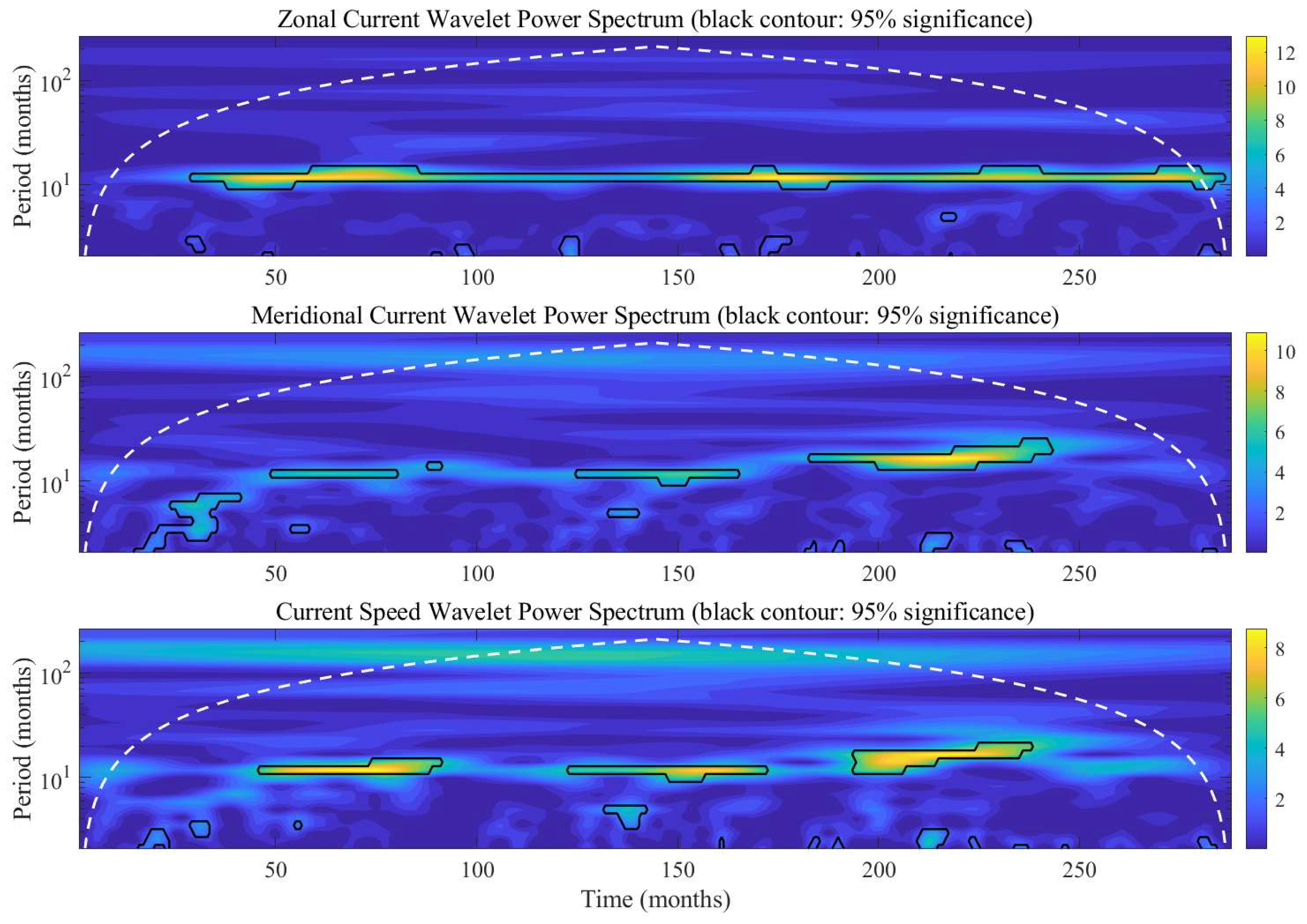
The results of the wavelet power spectrum analysis (Figure 18) show that significant periodic signals in the zonal velocity u are concentrated only in the 8–16-month seasonal and quasi-semiannual frequency bands, and passed the 95% significance test only during the two periods of 2005–2012 and 2018–2024. No significant interannual to decadal-scale periodic signals were identified during the study period; this finding is highly consistent with the results of the variance decomposition. For the meridional velocity v, high-power signals consistently passed the 95% significance test in the 8–16-month frequency band throughout the entire study period. This makes it the most stable seasonal component among all ocean current components, directly confirming that the annual cycle reversal of the East Asian monsoon is the core factor driving the seasonal circulation of meridional velocity in this region [23]. Furthermore, on the interdecadal timescale of approximately 150 months (12.5 years), a region of elevated wavelet power appears in the meridional current velocity, but it does not pass the 95% significance test against red noise. This suggests a possible influence of the Pacific Decadal Oscillation (PDO), but the limited data length precludes a definitive identification of a stable decadal period. [8]. Significant periodic signals in current magnitude are similarly concentrated in the 8–16-month annual cycle band, passing the 95% significance test for both the 2004–2012 and 2015–2024 periods; no significant interannual-scale periodic signals were detected.

3.2.4. Changes in the Characteristics of the Kuroshio Current’s Influx into the Luzon Strait

The Kuroshio intrusion zone in the Luzon Strait is the sole key channel for the exchange of water, heat, and momentum between the Pacific Ocean and the South China Sea. Variations in the intensity and path of this intrusion directly influence the circulation structure, temperature and salinity budgets, and mesoscale eddy activity in the northern South China Sea [48,49], and are sensitive to adjustments in large-scale circulation under global warming [50]. Selecting this region helps to complete the picture of Kuroshio penetration from the open ocean to the marginal sea and represents a key segment for elucidating the Kuroshio’s marginal sea effects.

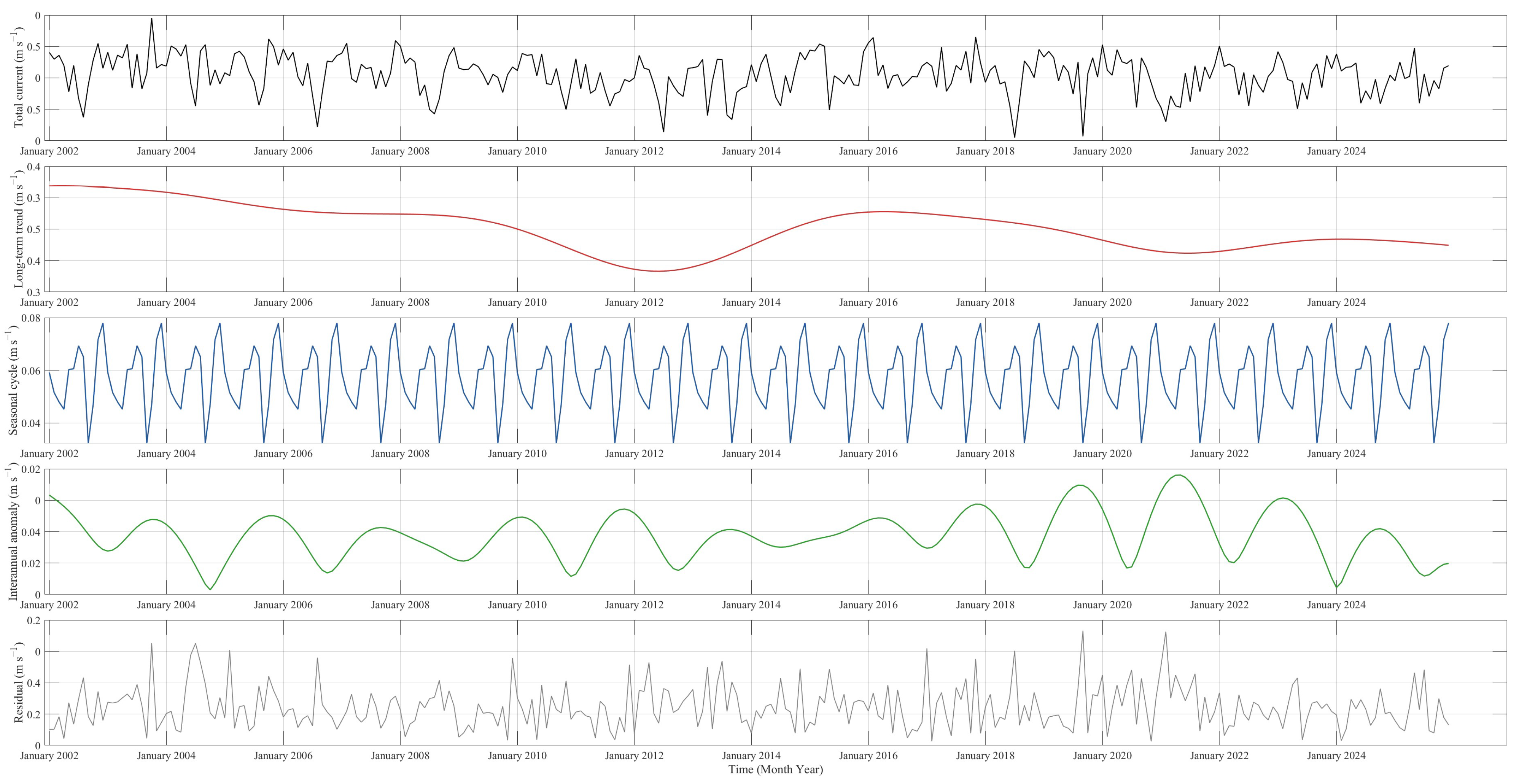
As shown in Figure 19, the total flow velocity of the Kuroshio intrusion current in the Luzon Strait remained stable between 0.2 and 0.7 m·s⁻¹ from 2002 to 2024, consistent with the typical velocity range for Kuroshio intrusion in this region. The temporal variations in flow velocity exhibit a composite pattern characterized by the superposition of seasonal oscillations, quasi-decadal interdecadal fluctuations, and high-frequency disturbances, indicating that the Kuroshio intrusion process is jointly regulated by dynamic processes at different scales [7]. The long-term low-frequency variation component extracted via a 60-month low-pass filter reveals the decadal evolution of Kuroshio intrusion intensity; this variation does not follow a simple linear trend but rather superimposes modulation signals from large-scale circulations such as the Pacific Decadal Oscillation (PDO) and the Kuroshio Great Bend [26]. This component exhibits a quasi-14-year oscillation pattern: the intrusion velocity decreased continuously from approximately 0.47 m·s⁻¹ during 2002–2012 to a trough value of 0.32 m·s⁻¹ in 2012, then rapidly rebounded to a peak of 0.43 m·s⁻¹ between 2012 and 2015, weakened again from 2015 to 2020, and has shown a slight upward trend since 2020; this overall evolution is consistent with the decadal adjustment patterns of the North Pacific subtropical circulation. The seasonal cycle component of the climate state exhibits exceptional stability, displaying interannual oscillations with a strict 12-month cycle. Its amplitude remains stable between 0.05 and 0.13 m·s⁻¹, and it is not significantly modulated by interannual signals, making it the most stable deterministic component driving ocean current variability in this region. The interannual anomaly component, separated by 24–60-month bandpass filtering, exhibits quasi-2–7-year oscillatory characteristics with an amplitude ranging from 0.01 to 0.04 m·s⁻¹. The amplitude has increased significantly since 2018, corresponding to the active phase of the El Niño–Southern Oscillation (ENSO) [26].

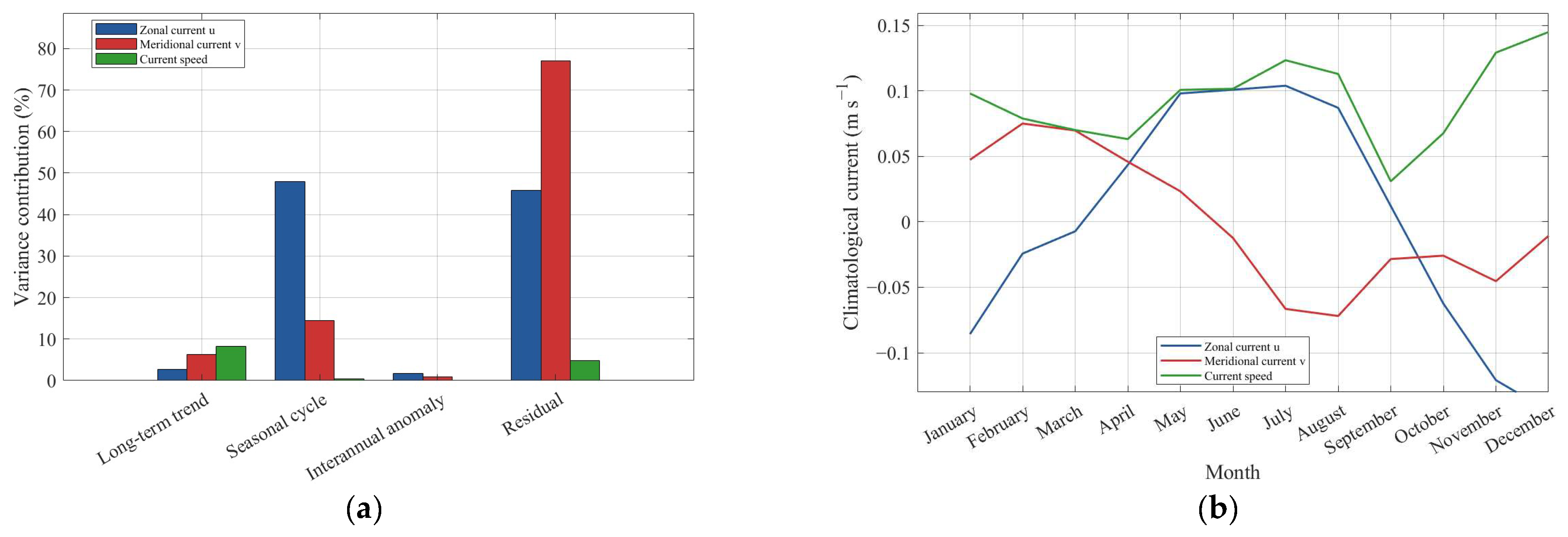
Based on the results of the variance decomposition (Figure 20), the variability in the zonal velocity u of the Kuroshio intrusion current in the Luzon Strait is overwhelmingly dominated by the climatic seasonal cycle, which accounts for 48% of the variance. followed by the high-frequency residual term, which contributes approximately 46%. The variance contributions from long-term trends and interannual anomalies are both less than 3%. This indicates that the spatiotemporal variability of the zonal flow in this region is primarily controlled by seasonal zonal adjustments driven by the East Asian monsoon and high-frequency mesoscale processes [51], while the modulating effects of large-scale circulation signals on the interannual to decadal scales are extremely weak. The variability characteristics of the meridional flow velocity v differ markedly from those of the zonal flow; the high-frequency residual term is its core dominant component [52], accounting for as much as 77% of the variance, while the climate-state seasonal cycle contributes approximately 14%, and the long-term trend and interannual anomalies contribute less than 6% and 1%, respectively. This characteristic aligns with the dynamical mechanism of Kuroshio intrusion into the Luzon Strait, where the meridional component of Kuroshio intrusion is strongly modulated by high-frequency dynamical processes such as mesoscale vortices and frontal instability, superimposed on the monsoon-driven seasonal signal. Regarding the variability in current velocity, the climate-mode seasonal cycle and the long-term trend are the primary contributing components, accounting for approximately 8.5% and 8% of the variance, respectively, while interannual anomalies contribute less than 1%, and the high-frequency residual term contributes about 5%; Combined with the variance decomposition characteristics of the vector components, it is evident that the seasonal variability in current velocity is primarily dominated by seasonal oscillations in the zonal flow, while the long-term trend reflects the regulatory effect of decadal variations in Kuroshio intrusion intensity on the regional average current velocity [49].

The multi-year average monthly climatological series for 2002–2024 clearly illustrates the seasonal dynamical characteristics of Kuroshio intrusion driven by the East Asian monsoon. The zonal flow velocity u exhibits a significant annual cycle reversal: during winter (December–February), under the influence of the northeastern monsoon, the zonal flow is negative and westward, reaching a maximum of approximately −0.08 m·s⁻¹ in January, corresponding to an enhanced westward intrusion of the Kuroshio into the South China Sea; In summer (June–August), the southwest monsoon prevails, and the zonal flow turns positive and easterly, reaching a maximum of approximately 0.10 m·s⁻¹ in July. At this time, the westward intrusion of the Kuroshio Current is suppressed, and water from the northern South China Sea flows eastward through the Luzon Strait; April and October mark the transitional periods between monsoon seasons, during which the zonal flow completes its seasonal reversal, consistent with the seasonal dynamical patterns formed by the monsoon-circulation system [53,54]. The meridional flow velocity v exhibits seasonal oscillations in antiphase with the zonal flow: During winter (January–March), when the zonal flow is westerly, the meridional flow is positive and northward, reaching a maximum of approximately 0.075 m·s⁻¹ in March, reflecting the northward deflection of the Kuroshio’s inflow branch driven by the northeastern monsoon; In summer (June–August), when the zonal flow is easterly, the meridional flow turns southward and negative, reaching a maximum of approximately −0.07 m·s^(−1) in August, as the southward South China Sea circulation driven by the southwest monsoon offsets the northward component of the intruding Kuroshio. The magnitude of the flow exhibits a bimodal seasonal variation, with generally weaker flow speeds in spring and autumn. Flow velocities are stronger in winter and summer, reaching an annual peak of approximately 0.145 m·s⁻¹ in December, exhibiting a general distribution pattern of weak flows in spring and autumn and strong flows in summer and winter. This pattern is consistent with the seasonal variations in the main Kuroshio current velocity and the seasonal evolution of water exchange fluxes in the Luzon Strait.

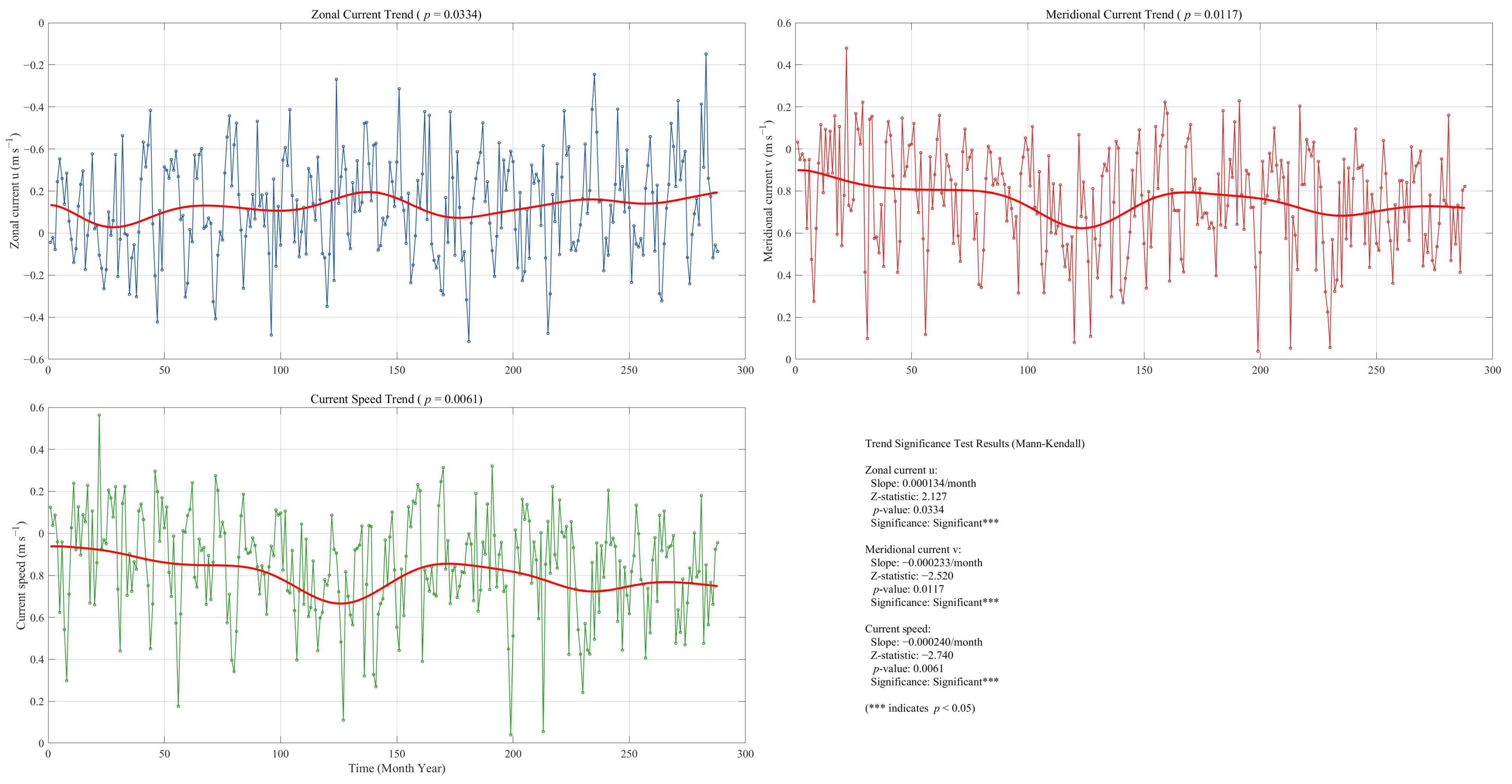
The results of the Mann–Kendall trend test (Figure 21) indicate that the zonal flow velocity u exhibits a statistically significant long-term increasing trend (p = 0.0334 < 0.05), with a trend slope of 0.000134 m·s⁻¹·month⁻¹ and an annual average increase of approximately 0.0016 m·s⁻¹· a⁻¹, indicating that the eastward component of the zonal ocean current in the study area continued to strengthen from 2002 to 2024. This corresponds to a weakening of the Kuroshio’s westward intrusion into the South China Sea during winter and a strengthening of its eastward outflow characteristics during summer, providing direct observational evidence for the long-term decline in the zonal component of the Kuroshio’s intrusion through the Luzon Strait [55,56]. The longitudinal current velocity v also exhibits a statistically significant long-term decreasing trend (p = 0.0117 < 0.05), with a trend slope of −0.000233 m·s⁻¹·month⁻¹ and an annual average decrease of approximately 0.0028 m·s⁻¹·year⁻¹. This reflects a sustained decline in the northward component of the meridional current in this region, directly indicating a long-term weakening of the northward branch of the Kuroshio’s intrusion into the South China Sea. The magnitude of the ocean current velocity also exhibits a significant long-term decreasing trend (p = 0.0061 < 0.01), with a trend slope of −0.000240 m·s⁻¹·month⁻¹ and an average annual decrease of approximately 0.0029 m·s⁻¹·year⁻¹. A comprehensive analysis of the trend characteristics of both zonal and meridional flow velocities reveals that the overall intensity of the Kuroshio intrusion into the Luzon Strait exhibited a highly significant long-term decline from 2002 to 2024. This conclusion is highly consistent with climate simulation results indicating that, against the backdrop of global warming, adjustments in the North Pacific subtropical circulation and the southward shift in the Kuroshio’s main axis have led to a weakening of the Kuroshio intrusion into the Luzon Strait [52,57].

Wavelet power spectrum analysis (Figure 22) indicates that the periodic characteristics of the various components of the Kuroshio intruding current in the Luzon Strait from 2002 to 2024 exhibit clear scale differentiation and temporal evolution patterns. The annual periodic signal in the zonal velocity u exhibited extremely strong statistical significance throughout the entire study period. The region of significance at the 95% confidence level spanned the entire time series, with a power peak as high as 12, fully confirming that the annual oscillation is the dominant mode of zonal flow variability. This result is fully consistent with the conclusion from variance contribution analysis that seasonal cycles play an absolutely dominant role [58]; No sustained, stable significant periodic signals were detected in the 20–40-month interannual scale range, further confirming that interannual variability makes a negligible contribution to the overall variability of the zonal flow. Significant periodic signals in the meridional flow velocity v are primarily concentrated in the 12–24-month seasonal and subseasonal scales. Specifically, high-power significant signals with periods of 12–18 months appeared from 2015 to 2022, with a peak of 10; while significant 12-month periodic signals appeared intermittently during 2005–2008 and 2010–2013. This indicates that the periodic variability of the meridional flow remains predominantly on the seasonal scale, but its signal stability is significantly lower than that of the zonal flow and is markedly modulated by decadal-scale processes [59], This characteristic is associated with the decadal evolution of mesoscale eddy activity in the Luzon Strait. No sustained significant signals were observed at the 30–80-month interannual and decadal scales, further confirming that interannual variability makes a relatively small contribution to the variability of the meridional flow. The dominant annual cycle for current velocity magnitude is also 12 months. High-power annual cycle signal zones formed during the three periods of 2004–2008, 2012–2016, and 2018–2024, with a power peak of 7, exhibiting intermittent enhancement characteristics. Furthermore, these high-power periods correspond to the timing of the strong El Niño events in 2006/2007, 2015/2016, and 2019/2020, revealing that ENSO exerts a significant interannual modulation on the seasonal cycle of ocean current intensity in this region [30,60]. Furthermore, a significant periodic signal in current velocity on an interannual timescale of 24–36 months emerged between 2018 and 2024, consistent with the increased amplitude of the interannual anomaly component, indicating a clear trend toward enhanced ENSO regulation of Kuroshio intrusion intensity in recent years.

To verify the robustness of the long-term weakening trend of Kuroshio intrusion in the Luzon Strait, we compared our results against two independent published datasets.

First, Wang et al. [48] applied an edge-detection method to satellite-derived sea surface temperature (SST) images combined with geostrophic currents from satellite altimetry (1993–2017) and independently confirmed that the Kuroshio intrusion into the Luzon Strait has exhibited a decreasing trend since the 1990s. Their reported current speed trend in the Luzon Strait closely matches the magnitude reported in this study.

Second, a systemwide weakening of the Kuroshio Current during 1993–2013 has been documented using eight independent data sets, including satellite altimetry, in situ hydrography, and reanalysis products [7,55]. This basin-scale weakening is consistent with the decreasing Kuroshio intrusion into the Luzon Strait reported here.

Furthermore, the same GLORYS12V1 reanalysis product has been widely validated in the Luzon Strait region by independent studies, showing good agreement with satellite altimetry and in situ observations for both mean state and interannual variability.

Taken together, these cross-validations support that the long-term weakening trend of Kuroshio intrusion into the Luzon Strait is a robust signal rather than an artifact of a single dataset or decomposition method.

The observed long-term weakening of the Kuroshio intrusion into the Luzon Strait can be physically linked to large-scale adjustments of the North Pacific subtropical circulation under global warming. Climate model simulations and reanalysis studies indicate that greenhouse warming drives a strengthened and poleward-shifted subtropical wind-driven gyre, accompanied by an intensified wind stress curl over the central North Pacific. This leads to a southward or eastward shift in the Kuroshio’s main axis east of Taiwan and a reduction in its westward penetration through the Luzon Strait.

Specifically, Wu et al. [56] attributed the weakening Kuroshio intrusion during the global warming hiatus (post-1998) to a weakening of the northeasterly monsoon and a reduced sea level tilt across the Luzon Strait. More recently, Chen et al. [58] showed that the decadal decline of Kuroshio intrusion since the 1990s is coherent with a broad-scale weakening of the Pacific subtropical circulation and a southward migration of the Kuroshio axis, both consistent with the response to a warming climate in Coupled Model Intercomparison Project phase 5 (CMIP5) projections.

In our results, the concurrent upstream strengthening of the North Equatorial Current bifurcation zone (Section 3.2.1) and the downstream weakening of the Luzon Strait intrusion are not contradictory. The NEC strengthening reflects enhanced westward transport of the tropical Pacific, while the Luzon Strait weakening is controlled by the meridional position and offshore shift in the Kuroshio’s main axis—a structural change rather than a simple transport decrease. This interpretation is supported by the significant eastward strengthening of the zonal velocity and northward weakening of the meridional velocity (Figure 20), which together indicate a rotation of the flow vector away from the Luzon Strait.

Thus, while our observational analysis cannot formally attribute causality, the identified trends are dynamically consistent with expected responses of the western boundary current–marginal sea system to a warming climate, as reported in multiple independent studies.

3.2.5. Correlation Analysis Between PDO and the Invasion Speed of the Kuroshio Current as Well as the NEC Speed PDO Modulation of Interannual Variability in NEC and Kuroshio Intrusion

A 13-month running mean was applied to the monthly NEC speed, Kuroshio intrusion velocity, and PDO index to isolate interannual variability from the seasonal cycle. Normalized anomalies reveal coherent covariability among the three fields throughout the 2002–2023 record, with concurrent positive excursions during the 2014–2016 warm PDO phase and negative anomalies during the 2020–2023 cold phase (Figure 23a). This visual correspondence indicates that basin-scale PDO forcing leaves a detectable imprint on both the equatorward western boundary current transport and the South China Sea inflow.

Correlation analysis confirms statistically significant linear relationships. The NEC speed averaged over 125–128° E, 13–16° N correlates with the PDO at r = 0.52 (p < 0.001), while the Kuroshio intrusion intensity in the Luzon Strait region (119–122° E, 19–22° N) exhibits a comparable coefficient of r = 0.54 (p < 0.001) (Figure 23b,c). The near-identical correlation magnitudes suggest that the PDO modulates the meridional migration of the NEC bifurcation and the westward penetration of the Kuroshio with roughly equal strength on interannual timescales.

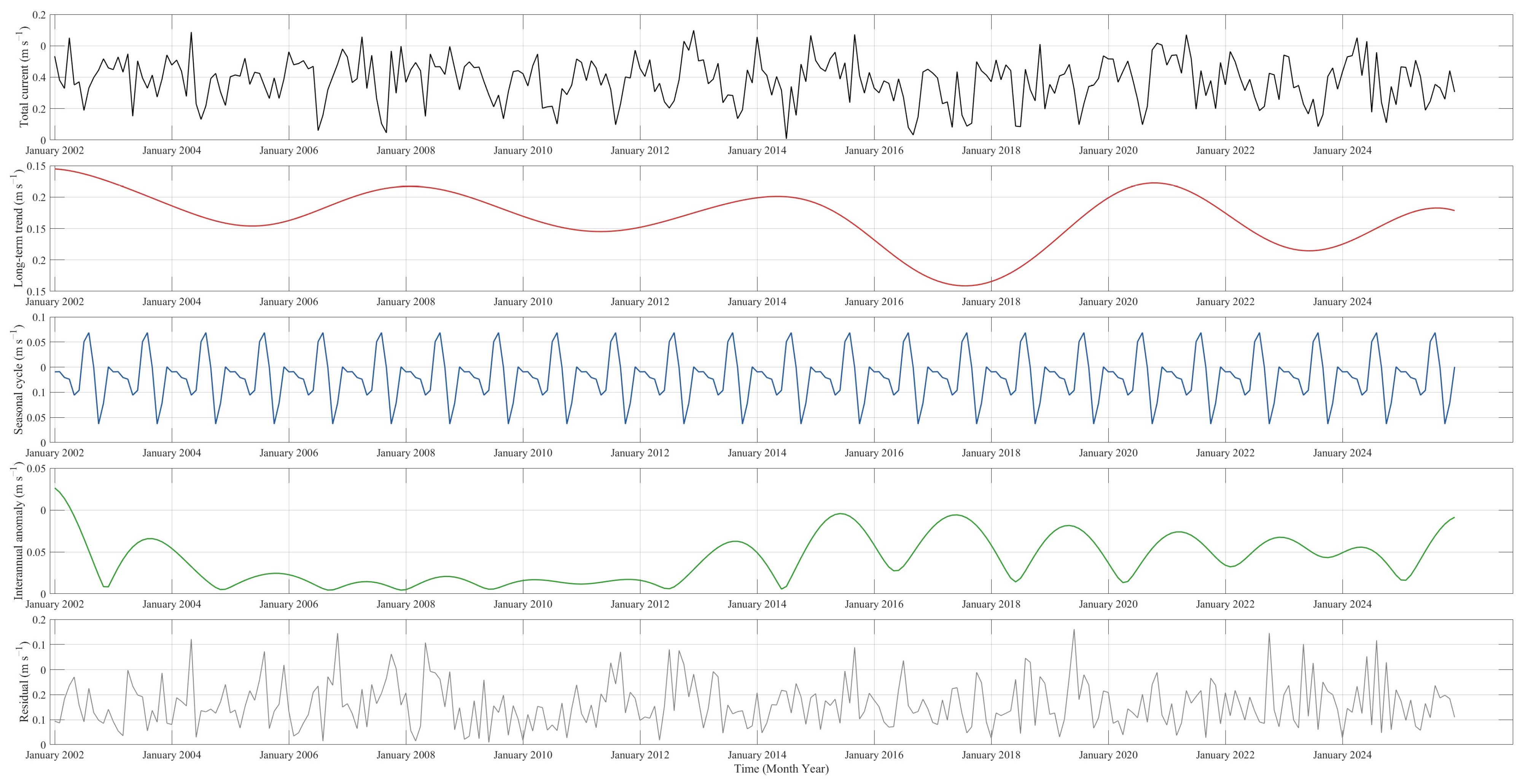
The synchronous response likely stems from large-scale wind field adjustments tied to PDO phase transitions. During warm PDO phases, anomalous anticyclonic circulation over the subtropical North Pacific weakens the trade winds in the western tropical Pacific, altering the Sverdrup transport and meridional pressure gradient that govern NEC bifurcation latitude. Concurrently, the relaxed wind forcing and associated sea level anomalies in the western Pacific enhance the pressure head driving Kuroshio water through the Luzon Strait. The comparable PDO sensitivities of both metrics underscore the dominant role of basin-scale climate forcing in coordinating regional circulation across the western tropical Pacific.

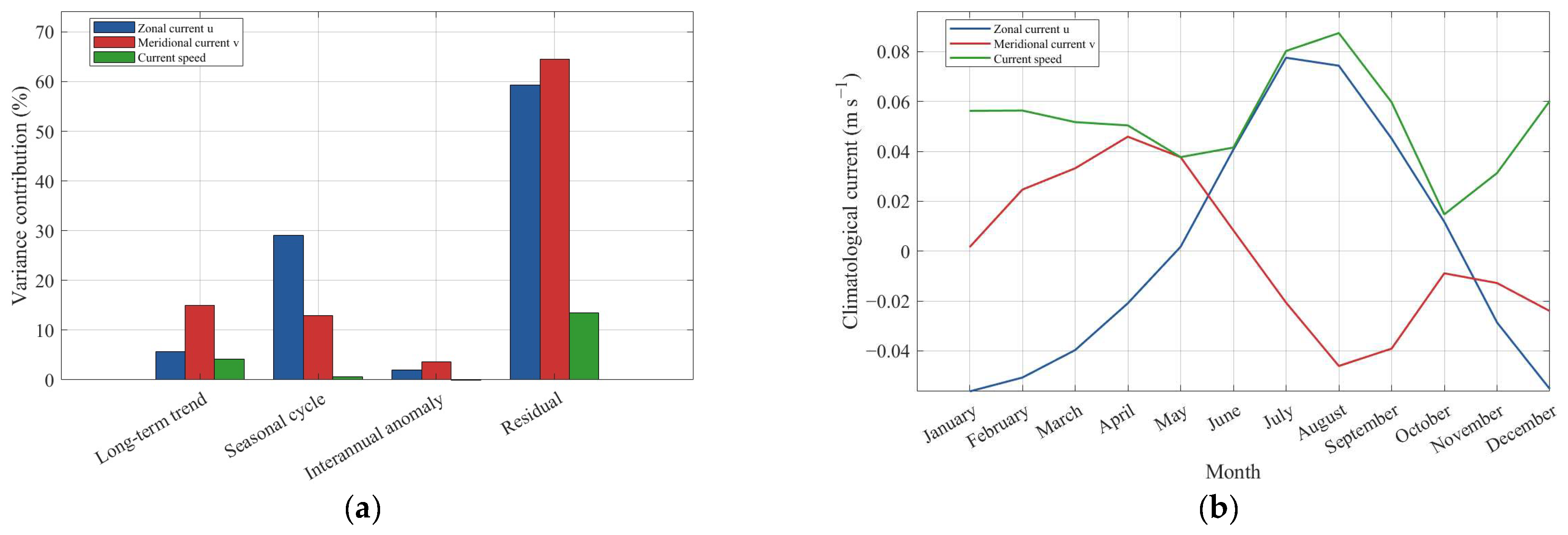
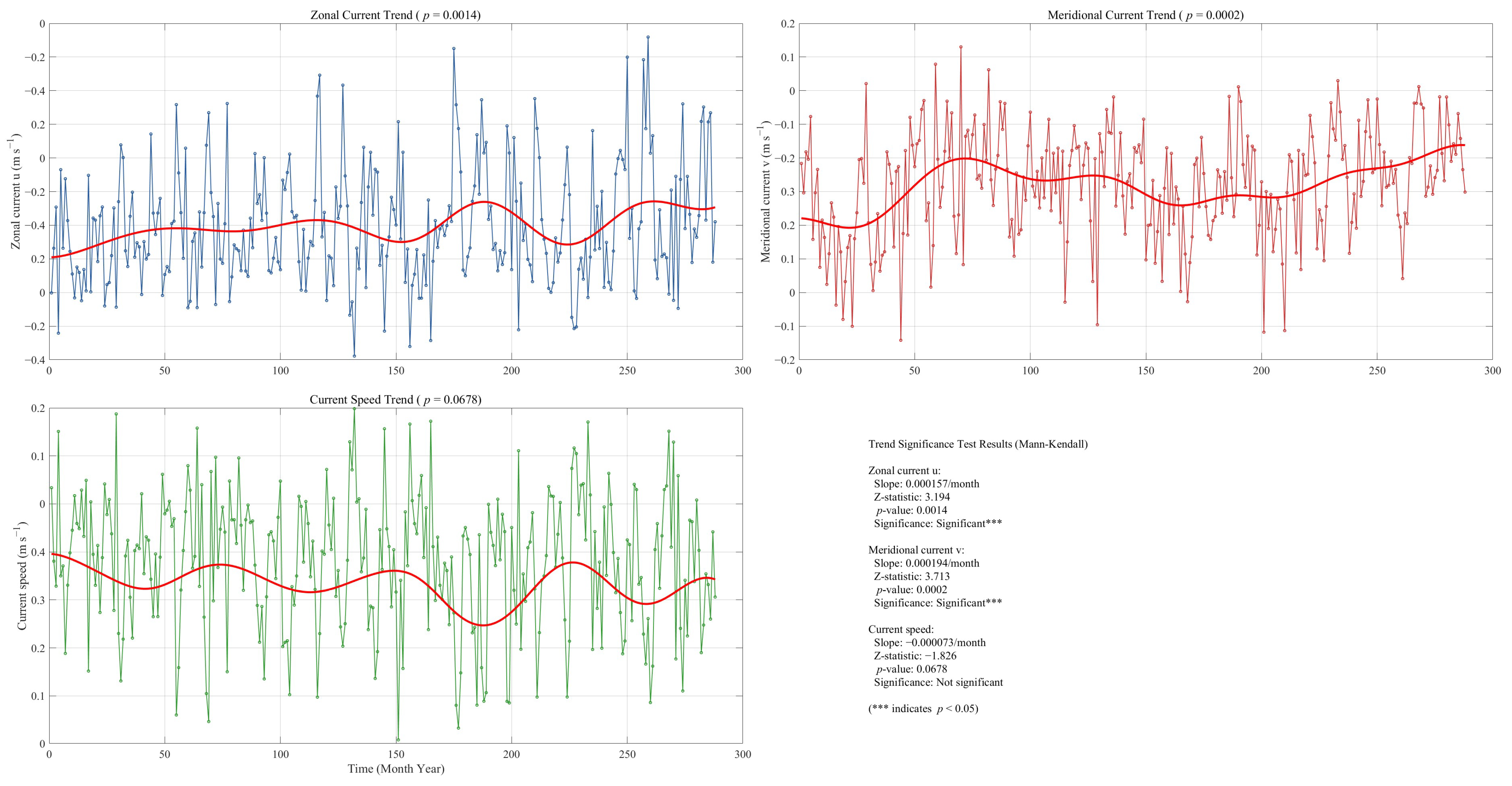
4. Conclusions

This study systematically investigates the multiscale variability characteristics and dynamical mechanisms of the Kuroshio Front east of Taiwan. It proposes and validates an adaptive iterative tracking algorithm based on flow field dynamical constraints, which significantly improves the accuracy and automation of the Kuroshio main axis extraction. The study selected four key sections: the North Equatorial Current bifurcation zone, the Kuroshio front east of Taiwan, the Kuroshio front in the East China Sea, and the Kuroshio intrusion zone in the Luzon Strait. Based on high-resolution reanalysis velocity fields from 2002 to 2024, a rigorous multiscale variability decomposition framework (including Fourier harmonics, Butterworth filtering, variance contribution decomposition, Mann–Kendall trend tests, and Morlet wavelet analysis) is introduced, systematically revealing the energy allocation, periodic structure, and long-term evolution patterns of current variability in each region. The main findings are as follows:

• In the North Equatorial Current bifurcation zone, zonal flow variability is dominated by seasonal cycles (29% variance contribution), while meridional flow shows notable low-frequency variability (15% variance contribution). Both zonal and meridional flows exhibit a significant strengthening trend (p < 0.01). Wavelet analysis indicates that zonal flow energy is concentrated in a 12-month cycle, whereas meridional flow exhibits low-frequency variability on timescales longer than ~8–10 years; however, a stable decadal period cannot be robustly identified given the 23-year data length.;
• In the Kuroshio Front east of Taiwan, high-frequency residuals (mesoscale vorticity) account for approximately 70% of the variance, indicating that mesoscale processes are the dominant driver (while the exact percentage has methodological uncertainties discussed in Section 2.4), with the seasonal cycle contributing about 22–25%; the magnitude of the velocity exhibits a semi-annual bimodal structure with higher values in winter and summer and lower values in spring and autumn, showing no significant long-term linear trend, while decadal oscillations are the primary form of low-frequency variation.
• In the Kuroshio Front region of the East China Sea, the seasonal circulation signal for meridional velocity is the most robust (contributing 25% of the variance), and the annual cycle persists throughout the entire period; significant cycles in zonal velocity and velocity magnitude appear only intermittently, and no long-term linear trends were detected.
• In the Kuroshio intrusion zone of the Luzon Strait, seasonal circulation dominates the variation in zonal flow (48%), while high-frequency residuals dominate the variation in meridional flow (77%); the magnitude of flow velocity exhibits a highly significant long-term declining trend (p < 0.01, with an average annual decrease of approximately 0.0029 m·s⁻¹·a⁻¹), accompanied by a strengthening of the easterly component and a weakening of the northerly component of the zonal flow, indicating a continuous weakening of the overall intensity of the Kuroshio intrusion into the South China Sea. Wavelet analysis further reveals significant interannual modulation of the seasonal cycle of flow velocity magnitude by ENSO.

In summary, this study overcomes the methodological limitations of traditional Kuroshio main axis extraction techniques, achieving high-precision automated tracking of the Kuroshio main axis. Mechanistically, it quantifies the long-term decaying trend in the intensity of Kuroshio intrusion into the Luzon Strait and the differentiated modulation modes of its vector components. The findings not only provide new observational evidence and a basis for assessing the multiscale dynamics of the Kuroshio front but also offer crucial support for understanding the evolution of western boundary current–marginal sea interactions in the context of global warming. Future research could further integrate high-resolution coupled models with long-term observational data to explore the pathways and feedback mechanisms through which Kuroshio variability influences regional climate and ecosystems.

References

1. Schneider, N. The role of sea surface temperatures in anchoring the Kuroshio and Gulf Stream Convergence Zones. In AGU Fall Meeting Abstracts; AGU: Washington, DC, USA, 2020; p. A055-03. [Google Scholar]
2. Xi, J.; Wang, Y.; Feng, Z.; Liu, Y.; Guo, X. Variability and Intensity of the Sea Surface Temperature Front Associated with the Kuroshio Extension. Front. Mar. Sci. 2022, 9, 836469. [Google Scholar] [CrossRef]
3. Zhou, G.; Li, Z.; Cheng, X. Intrinsic and wind-driven decadal variability of the Kuroshio Extension in altimeter observations. Front. Mar. Sci. 2021, 8, 766226. [Google Scholar] [CrossRef]
4. Fang, Y.-C.; Li, W.-T.; Chen, S.-H. Kuroshio path variability inferred from satellite-derived sea surface topography in the northwestern Pacific. Remote Sens. Environ. 2024, 315, 114443. [Google Scholar] [CrossRef]
5. Xu, W.; Zhang, L.; Wang, H.; Zhang, G. Spatiotemporal characterization and prediction of the subsurface temperature front of the Kuroshio extension. J. Sea Res. 2023, 196, 102444. [Google Scholar] [CrossRef]
6. Zhuang, Z.; Hui, Z.; Yang, G.; Zhao, X.; Yuan, Y. Principal-component estimates of the Kuroshio Current axis and path based on the mathematical verification between satellite altimeter and drifting buoy data. Acta Oceanol. Sin. 2020, 39, 14–24. [Google Scholar] [CrossRef]
7. Wang, H.; Zhang, Z.; Sun, Z.; Zhao, W. Interannual to decadal variations in different Kuroshio intrusion paths in the Luzon Strait based on long-term reanalysis data. J. Geophys. Res. Ocean. 2025, 130, e2024JC022155. [Google Scholar] [CrossRef]
8. Zhang, X.; Wang, B.; Wang, X.; Zhu, X.; Wu, B.; Sun, C. Interannual and decadal variations of the Kuroshio axis in the East China Sea. In Journal of Physics: Conference Series; IOP Publishing: Bristol, UK, 2023; Volume 2486, p. 012001. [Google Scholar]
9. Lellouche, J.-M.; Greiner, E.; Bourdallé-Badie, R.; Garric, G.; Melet, A.; Drévillon, M.; Bricaud, C.; Hamon, M.; Le Galloudec, O.; Regnier, C.; et al. The Copernicus Global 1/12° Oceanic and Sea Ice GLORYS12 Reanalysis. Front. Mar. Sci. 2021, 9, 698876. [Google Scholar] [CrossRef]
10. Thomson, R.E.; Emery, W.J. Data Analysis Methods in Physical Oceanography; Elsevier: Amsterdam, The Netherlands, 2024. [Google Scholar]
11. Liu, X.; Zhou, H.; Liu, H. Interannual variations of the north equatorial current across the Pacific Ocean. J. Geophys. Res. Ocean. 2024, 129, e2023JC020174. [Google Scholar] [CrossRef]
12. Wang, X.; Tong, B.; Wang, D.; Yang, L. Variations of the North Equatorial Current bifurcation and the SSH in the western Pacific associated with El Niño flavors. J. Geophys. Res. Ocean. 2020, 125, e2019JC015733. [Google Scholar] [CrossRef]
13. Weiss, T.L.; Linsley, B.K.; Gordon, A.L. Pacific North Equatorial Current bifurcation latitude and Kuroshio Current shifts since the Last Glacial Maximum inferred from a Sulu Sea thermocline reconstruction. Quat. Sci. Rev. 2021, 264, 106999. [Google Scholar] [CrossRef]
14. Wang, L.C.; Wu, C.R.; Qiu, B. Modulation of Rossby waves on the Pacific North Equatorial Current bifurcation associated with the 1976 climate regime shift. J. Geophys. Res. Ocean. 2014, 119, 6669–6679. [Google Scholar] [CrossRef]
15. Duan, J.; Li, Y.; Wang, F.; Chen, Z. Multidecadal change of the Mindanao Current: Is there a robust trend? Geophys. Res. Lett. 2019, 46, 6755–6764. [Google Scholar] [CrossRef]
16. Kim, Y.Y.; Qu, T.; Jensen, T.; Miyama, T.; Mitsudera, H.; Kang, H.W.; Ishida, A. Seasonal and interannual variations of the North Equatorial Current bifurcation in a high-resolution OGCM. J. Geophys. Res. Ocean. 2004, 109, 2003JC002013. [Google Scholar] [CrossRef]
17. Zhou, H.; Liu, X.; Li, R.; Wang, Y.; Yang, G. Intraseasonal variability of the North Equatorial Current bifurcation off the Philippines. J. Geophys. Res. Ocean. 2021, 126, e2021JC017646. [Google Scholar] [CrossRef]
18. Kang, S.M.; Watanabe, M.; Gayler, V. Common and distinct drivers of convective mass flux and Walker circulation changes. Geophys. Res. Lett. 2025, 52, e2024GL111897. [Google Scholar] [CrossRef]
19. Latif, M.; Bayr, T.; Kjellsson, J.; Lübbecke, J.F.; Martin, T.; Nnamchi, H.C.; Park, W.; Savita, A.; Sun, J.; Dommenget, D. Strengthening atmospheric circulation and trade winds slowed tropical Pacific surface warming. Commun. Earth Environ. 2023, 4, 249. [Google Scholar] [CrossRef]
20. McGregor, S.; Stuecker, M.F.; Kajtar, J.B.; England, M.H.; Collins, M. Model tropical Atlantic biases underpin diminished Pacific decadal variability. Nat. Clim. Change 2018, 8, 493–498. [Google Scholar] [CrossRef]
21. Wu, C.-R.; Lin, Y.-F.; Qiu, B. Impact of the Atlantic multidecadal oscillation on the Pacific North Equatorial Current bifurcation. Sci. Rep. 2019, 9, 2162. [Google Scholar] [CrossRef]
22. Li, J.; Gan, J. On the north equatorial current spatiotemporal modes and responses in the western boundary currents. Prog. Oceanogr. 2022, 205, 102820. [Google Scholar] [CrossRef]
23. Lee, S.; Na, H.; Min, H.S.; Kim, D.G.; Nakamura, H.; Nishina, A. Observational evidence of the Kuroshio meander and its propagation in the East China Sea. Front. Mar. Sci. 2025, 11, 1512572. [Google Scholar] [CrossRef]
24. Wang, S.; Guo, X.; Kido, S.; Qiao, Y.X.; Sasaki, H. Revisiting the Kuroshio frontal eddies in the East China Sea: Insights from the eddy energy budget. J. Geophys. Res. Ocean. 2025, 130, e2025JC022428. [Google Scholar] [CrossRef]
25. Nakamura, H.; Qiao, Y.-X.; Zhang, Z.-L.; Min, H.S.; Kim, D.G.; Park, J.-H.; Nishina, A.; Jeon, C.; Na, H.; Zhu, X.-H. Changes in the Speed of the Kuroshio in Response to Asian Monsoon Wind Stress Variability. J. Phys. Oceanogr. 2025, 55, 1507–1520. [Google Scholar] [CrossRef]
26. Tseng, Y.H.; Ho, C.R.; Zheng, Q.; Zheng, Z.W. Loop current west of the Luzon strait triggered by Kuroshio cut-off events east of Taiwan Island. J. Geophys. Res. Ocean. 2025, 130, e2024JC021572. [Google Scholar] [CrossRef]
27. Qiao, Y.-X.; Nakamura, H.; Kako, S.; Nishina, A.; Tomita, T. Synchronized decadal variabilities in the Kuroshio and Kuroshio Extension system. Prog. Oceanogr. 2022, 204, 102808. [Google Scholar] [CrossRef]
28. Wang, Y.-L.; Wu, C.-R. Discordant multi-decadal trend in the intensity of the Kuroshio along its path during 1993–2013. Sci. Rep. 2018, 8, 14633. [Google Scholar] [CrossRef]
29. Chang, Y.-L.; Oey, L.Y. Interannual and seasonal variations of Kuroshio transport east of Taiwan inferred from 29 years of tide-gauge data. Geophys. Res. Lett. 2011, 38, L08603. [Google Scholar] [CrossRef]
30. Kuo, Y.-C.; Tseng, Y.-H. Influence of anomalous low-level circulation on the Kuroshio in the Luzon Strait during ENSO. Ocean Model. 2021, 159, 101759. [Google Scholar] [CrossRef]
31. Wang, Q.; Yuan, X.; Hu, D.; Sasaki, H. Stronger intraseasonal variability observed below the seasonal thermocline in the Kuroshio east of Taiwan during 2014 and 2015. J. Geophys. Res. Ocean. 2021, 126, e2021JC017194. [Google Scholar] [CrossRef]
32. Ren, Q.; Yu, F.; Nan, F.; Li, Y.; Wang, J.; Liu, Y.; Chen, Z. Effects of mesoscale eddies on intraseasonal variability of intermediate water east of Taiwan. Sci. Rep. 2022, 12, 9182. [Google Scholar] [CrossRef] [PubMed]
33. Chang, M.-H.; Jan, S.; Mensah, V.; Andres, M.; Rainville, L.; Yang, Y.J.; Cheng, Y.-H. Zonal migration and transport variations of the Kuroshio east of Taiwan induced by eddy impingements. Deep Sea Res. Part I Oceanogr. Res. Pap. 2018, 131, 1–15. [Google Scholar] [CrossRef]
34. Isobe, A.; Kamachi, M.; Masumoto, Y.; Uchida, H.; Kuragano, T. Seasonality of the Kuroshio transport revealed in a Kuroshio assimilation system. J. Oceanogr. 2004, 60, 321–328. [Google Scholar] [CrossRef]
35. Hsin, Y.C.; Qiu, B.; Chiang, T.L.; Wu, C.R. Seasonal to interannual variations in the intensity and central position of the surface Kuroshio east of Taiwan. J. Geophys. Res. Ocean. 2013, 118, 4305–4316. [Google Scholar] [CrossRef]
36. Miyazawa, Y.; Zhang, R.; Guo, X.; Tamura, H.; Ambe, D.; Lee, J.S.; Okuno, A.; Yoshinari, H.; Setou, T.; Komatsu, K. Water mass variability in the western North Pacific detected in a 15-year eddy resolving ocean reanalysis. J. Oceanogr. 2009, 65, 737–756. [Google Scholar] [CrossRef]
37. Wu, C.-R.; Wang, Y.-L.; Chao, S.-Y. Disassociation of the Kuroshio current with the Pacific decadal oscillation since 1999. Remote Sens. 2019, 11, 276. [Google Scholar] [CrossRef]
38. As, M.A.A.; Lee, S.-Y.; Liu, C.-Y. Comprehensive Analysis of Trends in Ocean Surface Current by Delineating Kuroshio Extent Using an Optimized Segmentation Algorithm. IEEE Access 2024, 12, 177468–177490. [Google Scholar] [CrossRef]
39. Wang, Q. Revisiting the relationship between the North Pacific decadal variability and the Kuroshio Extension bimodality. In Proceedings of the European Geosciences Union General Assembly 2024 (EGU24), Vienna, Austria, 14–19 April 2024; p. 7259. [Google Scholar]
40. Qiu, B.; Chen, S. A new dynamic regime in the Kuroshio/Kuroshio extension and the North Pacific Climate System After 2018. J. Clim. 2026, 39, 349–362. [Google Scholar] [CrossRef]
41. Wang, H.; Liu, Q.; Yan, H.; Song, B.; Zhang, W. The interactions between surface Kuroshio transport and the eddy field east of Taiwan using satellite altimeter data. Acta Oceanol. Sin. 2019, 38, 116–125. [Google Scholar] [CrossRef]
42. Chen, J.; Zhu, X.-H.; Zheng, H.; Wang, M. Submesoscale dynamics accompanying the Kuroshio in the East China Sea. Front. Mar. Sci. 2023, 9, 1124457. [Google Scholar] [CrossRef]
43. Ito, D.; Kodama, T.; Shimizu, Y.; Setou, T.; Hidaka, K.; Ambe, D.; Sogawa, S. Frontogenesis elevates the maximum chlorophyll a Concentration at the subsurface near the Kuroshio during well-stratified seasons. J. Geophys. Res. Ocean. 2023, 128, e2022JC018940. [Google Scholar] [CrossRef]
44. Qiao, Y.X.; Nakamura, H.; Tomita, T.; Kako, S.; Nishina, A.; Zhu, X.H.; Liu, Z.J. ENSO-related interannual variability of the Kuroshio in the East China Sea since the mid-2000s. J. Geophys. Res. Ocean. 2023, 128, e2023JC019749. [Google Scholar] [CrossRef]
45. Yan, X.; Kang, D.; Curchitser, E.N.; Liu, X.; Pang, C.; Zhang, L. Seasonal variability of eddy kinetic energy along the Kuroshio Current. J. Phys. Oceanogr. 2023, 53, 1731–1752. [Google Scholar] [CrossRef]
46. Wang, L.; Zhong, Y. Spatially-varying Kuroshio surface water intrusion into the East China Sea shelf on seasonal and interannual time scales. Acta Oceanol. Sin. 2025, 44, 20–31. [Google Scholar] [CrossRef]
47. Zhang, L.; Xu, W.; Ma, X.; Li, M. Predictability Study of the Kuroshio Front in the East China Sea Based on In-Situ Observational Data: Analysis and Prediction Using Mann-Kendall Test and CNN-LSTM-Attention. In International Conference on Advances in Civil and Ecological Engineering Research; Springer: Berlin, Germany, 2024; pp. 511–528. [Google Scholar]
48. Wen, L.; Kang, S.; Li, X. The impact of the western boundary Kuroshio current on dissolved organic nitrogen cycling in the South China Sea. In Proceedings of the EGU General Assembly Conference Abstracts, Vienna, Austria, 27 April–2 May 2025. [Google Scholar]
49. Chang, Y.; Shih, Y.-Y.; Tsai, Y.-C.; Lu, Y.-H.; Liu, J.T.; Hsu, T.-Y.; Yang, J.-H.; Wu, X.-H.; Hung, C.-C. Decreasing trend of kuroshio intrusion and its effect on the chlorophyll-a concentration in the Luzon Strait, South China Sea. GISci. Remote Sens. 2022, 59, 633–647. [Google Scholar] [CrossRef]
50. Li, W.; Shang, Y.; Li, C.; Xu, C.; Laws, E.A.; Liu, X.; Huang, B. A stronger Kuroshio intrusion leads to higher chlorophyll a concentration in the northern South China Sea. J. Geophys. Res. Ocean. 2025, 130, e2024JC021389. [Google Scholar] [CrossRef]
51. He, Z.; Fu, X.; Zhao, Y.; Jiang, X. Multiscale Energy Transfers and Conversions of Kuroshio in Luzon Strait and Its Adjacent Regions. J. Mar. Sci. Eng. 2022, 10, 975. [Google Scholar] [CrossRef]
52. Yang, Q.; Liu, H.; Lin, P. The effect of oceanic mesoscale eddies on the looping path of the Kuroshio intrusion in the Luzon Strait. Sci. Rep. 2020, 10, 636. [Google Scholar] [CrossRef]
53. Zheng, H.; Zhu, X.H. Water exchange through the upper and middle Luzon Strait using the sigma–pi diagram. J. Geophys. Res. Ocean. 2024, 129, e2024JC021092. [Google Scholar] [CrossRef]
54. Zhao, R.; Zhu, X.-H.; Zhang, C.; Zheng, H.; Zhu, Z.-N.; Ren, Q.; Liu, Y.; Nan, F.; Yu, F. Summer anticyclonic eddies carrying Kuroshio waters observed by a large CPIES array west of the Luzon Strait. J. Phys. Oceanogr. 2023, 53, 341–359. [Google Scholar] [CrossRef]
55. Wu, B.; Gan, J.; Lin, X.; Qiu, B. Long-term decreasing of sea level along latitude of the Luzon Strait during 1993–2020: Surface versus subsurface perspectives. J. Geophys. Res. Ocean. 2024, 129, e2023JC019805. [Google Scholar] [CrossRef]
56. Wu, B.; Gan, J. Long-term variation of the eddy kinetic energy in the Northeastern South China sea. Prog. Oceanogr. 2024, 229, 103366. [Google Scholar] [CrossRef]
57. Wu, C.-R.; Wang, Y.-L.; Lin, Y.-F.; Chiang, T.-L.; Wu, C.-C. Weakening of the Kuroshio intrusion into the South China Sea under the global warming hiatus. IEEE J. Sel. Top. Appl. Earth Obs. Remote Sens. 2016, 9, 5064–5070. [Google Scholar] [CrossRef]
58. Zhong, Y.; Zhou, M.; Waniek, J.J.; Zhou, L.; Zhang, Z. Seasonal variation of the surface Kuroshio intrusion into the South China Sea evidenced by satellite geostrophic streamlines. J. Phys. Oceanogr. 2021, 51, 2705–2718. [Google Scholar] [CrossRef]
59. Chen, Y.; Zhai, F.; Li, P. Decadal variation of the Kuroshio intrusion into the South China Sea during 1992–2016. J. Geophys. Res. Ocean. 2020, 125, e2019JC015699. [Google Scholar] [CrossRef]
60. Lin, K.; Han, T.; Zhang, Y.; Shen, C.C.; Lee, S.Y.; Wang, J.; Mohtar, A.T.; Huang, K.F.; Chiang, H.W.; Chen, Y.G.; et al. Influences of east Asian winter monsoon and El Niño-Southern Oscillation variability on the Kuroshio intrusion to the South China Sea over the past 60 years. Geophys. Res. Lett. 2024, 51, e2023GL104155. [Google Scholar] [CrossRef]
Figure 1. Schematic Diagram of the Kuroshio Current Main Axis Extraction.
Oceans 07 00049 g001
Figure 2. Schematic diagram of the Kuroshio Main Branch extraction results (the magnified area shows the Kuroshio Extension).
Oceans 07 00049 g002
Figure 3. The velocity profiles along the main axis.
Oceans 07 00049 g003
Figure 4. Comparison of Kuroshio Spindle Extraction Methods. M1 is the proposed adaptive iterative tracking algorithm (dynamic vertical search); M2 is the traditional maximum velocity tracking; M3 and M4 are other reference methods.
Oceans 07 00049 g004
Figure 5. (a) Frequency distribution map of sea surface temperature gradients from winter 2002 to 2024 (The colors range from red to blue, indicating decreasing frequency of temperature fronts.); (b) Main axis of the Kuroshio current identified by the M1 method (Black solid line).
Oceans 07 00049 g005
Figure 6. The study areas selected for this paper. (A) The Pacific NEC branching zone, (B) The Kuroshio Front east of Taiwan, (C) The East China Sea Kuroshio Front, (D) The Kuroshio intrusion zone in the Luzon Strait.
Oceans 07 00049 g006
Figure 7. Time Series Decomposition of Flow Velocities at the Forking Region of the NEC in the North Pacific Ocean.
Oceans 07 00049 g007
Figure 8. (a) Contributions to the variance in current velocity in the branching zone of the North Equatorial Current (NEC) in the North Pacific and (b) multi-year monthly averages.
Oceans 07 00049 g008
Figure 9. Trends in Current Velocity and Significance Analysis in the Fork Region of the North Equatorial Current (NEC) in the North Pacific.
Oceans 07 00049 g009
Figure 10. Wavelet Spectrum Analysis of Current Velocity in the Forking Region of the North Equatorial Current (NEC) in the North Pacific. (Note: Wavelet power at timescales >100 months does not reach the 95% significance level; see Section 3.2.1 for interpretation.).
Oceans 07 00049 g010
Figure 11. Time-Series Decomposition of Flow Velocity in the Kuroshio Front Region off Taiwan.
Oceans 07 00049 g011
Figure 12. (a) Contribution of Flow Velocity Variance to the Kuroshio Front Zone in Taiwan and (b) Long-Term Monthly Averages.
Oceans 07 00049 g012
Figure 13. Trends in Current Velocity and Significance Analysis in the Kuroshio Front East of Taiwan.
Oceans 07 00049 g013
Figure 14. Spectral Analysis of Small-Scale Flow Velocity in the Kuroshio Front East of Taiwan.
Oceans 07 00049 g014
Figure 15. Time-Series Decomposition of Current Velocity in the Kuroshio Front of the East China Sea.
Oceans 07 00049 g015
Figure 16. (a) Contribution of Variance in Current Velocity in the Kuroshio Front Zone of the East China Sea and (b) Multi-Year Monthly Averages.
Oceans 07 00049 g016
Figure 17. Trends and Significance Analysis of Current Velocity in the Kuroshio Front Zone of the East China Sea.
Oceans 07 00049 g017
Figure 18. Spectral Analysis of Small-Scale Flow Velocity in the Kuroshio Front of the East China Sea.
Oceans 07 00049 g018
Figure 19. Time-series decomposition of current velocities in the Luzon Strait.
Oceans 07 00049 g019
Figure 20. (a) Contributions to the Variance of Current Velocity in the Luzon Strait and (b) Multi-Year Monthly Averages.
Oceans 07 00049 g020
Figure 21. Trends in Current Velocity and Significance Analysis in the Luzon Strait.
Oceans 07 00049 g021
Figure 22. Wavelet Spectrum Analysis of Current Velocity in the Luzon Strait.
Oceans 07 00049 g022
Figure 23. Correlation Analysis Between PDO and the Invasion Speed of the Kuroshio Current as Well as the NEC Speed.
Oceans 07 00049 g023