


Abstract
Railroad daily operations can be significantly disrupted by unforeseen events such as adverse weather conditions and train accidents. These events often result in delays in delivering shipments on time. Therefore, studying how to reschedule freight trains during emergencies is essential for enhancing the competitiveness of rail transportation products. This paper proposed a method specifically designed for the rescheduling of freight trains, aiming to simultaneously modify the train operation plan and dynamically adjust railcar flow routes in response to unexpected events. The problem was formulated with a multi-objective model based on a two-layer space–time network. To accurately measure schedule deviations, we introduced a set of indicators specifically tailored to the characteristics of railroad freight transportation. The ε-constraint method was employed to establish a framework for searching three-dimensional Pareto solutions. Computational experiments were performed on a Chinese railroad network. The results validated the effectiveness and applicability of the proposed methodology.
1. Introduction
Rail freight transportation involves a sophisticated operational process and consumes substantial resources, including locomotives and railcars [1]. To ensure the efficient allocation of resources, which fulfills economic objectives and expedites customer service, railroads must develop comprehensive plans that cover both external and internal aspects. Externally, the railroad company presents a service plan (presented as a timetable) to potential customers. Meanwhile, internal operations, not visible to customers, involve decisions such as car routing (determining the physical route for each origin–destination shipment) [2], car-to-block assignment (deciding which blocks should be built and the serving block sequence for each OD’s shipments) [3] and block-to-train assignment [4].
While the decisions above provide a strategic and tactical foundation for daily railway operations, at the operational level, railroad dispatchers must still formulate daily operation plans to regulate real-time train and railcar transportation organization. Constrained by freight capacity, many railways, including China’s rail system, adopt a controlled transportation organization mode in which freight trains can depart only when minimum marshaling size requirements are satisfied. Nevertheless, conventional freight train timetables are generally compiled based on medium- and long-term freight volume forecasts [5], which cannot fully match the real-time dynamic accumulation of railcars. When the actually accumulated railcars fail to reach the target train size, pre-planned timetable schemes cannot be implemented as scheduled. Accordingly, dispatchers need to develop a technical document known as the train operation plan based on dynamic railcar data before each day’s work. The train operation plan comprises two main components: (1) establishing the time–space routes for freight trains, which involves determining the time schedules for trains [6], and (2) establishing the time–space routes for railcars, which involves creating transportation schemes to assign railcars to specific trains [7].
Under normal circumstances, dispatchers operate trains according to the established train operation plan. However, external and internal factors such as adverse weather conditions and malfunctions in the railroad infrastructure can lead to situations where trains are either early, late, canceled, or added [8]. As a result, railcars may fail to reach their destinations according to the established plan and could become stranded along the route. In such instances, dispatchers must promptly adjust the train operation plan to restore regular shipment transportation. However, relying solely on dispatchers’ experience and subjective judgment to make temporary adjustments to the train operation plan is arbitrary. Furthermore, the railroad company has already committed to delivering the shipments within a specified deadline after accepting the order. Failing to adjust the train operation plan promptly could disrupt the on-time delivery of the shipments, which is not conducive to enhancing the competitiveness of railroads in the freight market. Therefore, there is an urgent need to propose an automated method of plan adjustment to effectively cope with the negative impact of unexpected conditions on rail freight operations.
Addressing this need is complicated by the fact that the operational environment of freight railroads varies significantly across regions, which directly shapes the rescheduling problem. In Europe, for instance, railroads typically operate on a scheduled-service basis, where trains run according to fixed timetables without strict composition requirements. In the United States, freight trains predominantly operate on dedicated freight lines. This study is situated in a mixed-traffic railway system in which freight trains are subject to minimum marshaling size requirements and their operations are tightly coupled with passenger train schedules and railcar flow movements. In this setting, because train departures depend on sufficient car accumulation while car routing must conform to available train schedules, the two decisions—adjusting train schedules and reassigning railcars to trains—are tightly interdependent and cannot be handled in isolation.
Despite this strong interdependence, the joint adjustment of these two decisions remains insufficiently addressed in the literature. Existing studies on train rescheduling have largely focused on passenger railways or treated them as separable sub-problems, overlooking their coupling in freight operations. This is partly because railcar routing at the operational level involves a richer set of activities than train scheduling alone, including the transition between loaded and empty car states, empty car distribution, and loaded car transportation, which have not been considered in prior studies. Prior service network design research [9] employed a multi-layer space–time network to characterize the movements of railcars and trains, but that work operates at the tactical level and its car layer is too simple to fully capture the car organization process, including the handling of empty cars, which renders it inadequate for daily freight operations. To bridge this gap, this paper investigates the integrated adjustment of train operation plans under disruptions. Specifically, we address the following research questions: (i) How can the coupling between freight train rescheduling and railcar-to-train reassignment be systematically modeled within an effective joint optimization framework? (ii) How can an effective trade-off between customer interests and operator interests be achieved during the adjustment process? To answer these questions, we construct a two-layer space–time network tailored to freight operations and propose a comprehensive optimization method. By refining the space–time arc types to explicitly capture the complete turnover process of railcars, this network structure enables the simultaneous optimization of train rescheduling and railcar routing under disruptions. In particular, a three-dimensional Pareto search framework is developed to capture the trade-offs among the conflicting objectives.
The remainder of this paper is organized as follows. Section 2 reviews the related literature. Section 3 presents the problem description, model formulation, and solution algorithm in detail. Section 4 reports experimental results and discussion. Section 5 concludes the study and outlines future research directions.
2. Literature Review
2.1. Train Scheduling
The train scheduling problem has been extensively proven to be NP-hard [10,11]. Early research predominantly focused on constructing conflict-free space–time trajectories for trains on single or multi-track lines. Some papers did not explicitly differentiate between freight and passenger trains and implicitly included freight train scheduling in their problem formulation [12,13,14,15]. Other papers explicitly addressed the freight train scheduling problem [6,16,17,18,19,20,21,22]. Jovanović and Harker [16] developed the SCAN I decision-support system for tactical freight train scheduling, and Kraay and Harker [17] proposed a real-time freight train scheduling model linking tactical plans with line dispatching. While these contributions laid the methodological foundation, particularly in space–time network modeling, they implicitly assumed that once a train path is laid out in the timetable, it can be fully realized in practice. However, a series of questions remain unanswered: which specific freight should each train carry, where should the empty cars for loading come from, and how should the empty cars generated after unloading be redistributed? These are precisely the issues that dynamic railcar flow routing needs to address. Addressing these questions is particularly necessary in countries with strict train operation requirements, because the allocation of car flow directly determines the size of the trains to be operated, which, in turn, determines whether the timetable can be realized in actual operations.
Although some scholars have considered delays in the delivery of shipments when scheduling trains, implicitly considering the coupling between railcars and trains [6], they assume that sufficient empty railcars are always available for loading, and, thus, empty railcar allocation decisions are not embedded within the model. In practice, empty railcar repositioning constitutes a substantial component of daily railway operations. Unlike loaded railcars, empty railcars have no fixed flow directions, which necessitates holistic decision-making that jointly considers freight demand and the time and locations at which empty railcars are released. Accordingly, the integrated optimization of train scheduling and railcar flow routing for both loaded and empty railcars represents a critical research gap that demands attention.
2.2. Train Rescheduling Under Disruptions
When unexpected events disrupt railway operations, dispatchers must rapidly adjust the pre-planned timetable to restore feasibility. A rich body of literature has explored measures including retiming [23], reordering [24], canceling [25,26], adding [27,28], rerouting [27,29], and flexible stopping [30,31]. A common feature of these studies is their focus on adjusting macro-level timetable parameters. However, most of these model architectures were developed for passenger railways and are not directly transferable to freight operations. First, on lines shared by both passenger and freight trains, passenger trains are given higher operational priority, so freight train rescheduling is rigidly constrained by passenger train timetables. Second, unlike passenger operations, where boarding, alighting, and transferring are executed by passengers themselves, freight operations require railway authorities to organize loading, transportation, transshipment, and unloading. Consequently, practical constraints such as transshipment time requirements and empty railcar supply must be incorporated into the rescheduling model.
Some studies have addressed freight train operations under disruptions. Haque, et al. [32] developed a rolling-horizon mixed-integer linear programming framework for the real-time integrated rescheduling of freight services and track assignment. Wang, et al. [33] focused on the problem of coordinated rescheduling of train timetable and crew scheme in the presence of disruptions on a double-track passenger–freight collinear railway. However, these studies primarily focus on optimizing the utilization of infrastructure resources and crew scheduling when rescheduling trains. Qu and He [7] developed a time–space network model and an improved A* algorithm to predict and control station traffic congestion under emergency conditions, considering the redistribution of dynamic railcar flows. Nevertheless, their model assumes that the train timetable remains fixed and only adjusts railcar flow routing results. In essence, this approach merely modifies train composition without adjusting train paths in the timetable.
Therefore, a critical research gap remains: no model jointly integrates train rescheduling and railcar flow rerouting under disruptions, notwithstanding their tight interdependence in real-world operations. Rescheduling trains without reallocating their constituent railcars may fail to adequately ensure transportation efficiency and, at the same time, may produce infeasible timetables that do not satisfy the required train marshaling constraints.
2.3. Research Comparison
From the perspective of optimization objectives, the literature on train rescheduling can be categorized into customer-centric and operator-centric approaches. The former aims to minimize the impact on customers, such as travel delays and missed connections, while the latter focuses on reducing operational costs. In the operator-centric category, Ghaemi, et al. [34] developed a MILP model for the optimal short-turning of trains during complete blockages, which determines the optimal station and timing for short-turning affected trains while considering traffic interaction on both sides of the disruption. Altazin, et al. [35] proposed a multi-objective optimization–simulation approach for real-time rescheduling in dense railway systems, optimizing recovery time, passenger service quality, and the number of operational decisions simultaneously. In the customer-centric category, Corman, et al. [36] developed microscopic passenger-centric models with decomposition-based heuristics and min-cost flow lower bounds. Dollevoet and Huisman [37] developed an iterative heuristic for large-scale delay management that accounts for passenger rerouting behavior by iteratively updating classical model parameters. Besides focusing on mitigating the impact of plan adjustments on customers, Majumder et al. [38] further proposed a data-driven framework using machine learning and rule-based techniques to quantify railway service quality, offering a complementary perspective for evaluating rescheduling outcomes.
Our paper considers both perspectives by simultaneously optimizing operational costs, plan deviation, and freight transportation efficiency. Table 1 compares our paper with related publications, categorizing them as operator-centric, customer-centric, or both. It can be found that our paper extends previous research in the following aspects:
Table 1.
Summary of relevant studies.
- (1)
- The formulated model incorporates two decisions, adjusting the space–time routes of both freight trains and railcars, an issue that no reviewed study jointly optimizes under disruptions.
- (2)
- Most studies have only considered a single scenario, such as station disruptions, track or segment blockage, and train delays. Our paper designs multiple scenarios of unexpected events in the case study, including scenarios that are unique to freight operations, such as changes in transportation demand, thereby demonstrating the scalability of the proposed method across different types of disturbances.
3. Materials and Methods
3.1. Problem Description
3.1.1. Dynamic Railcar Flow Routing
Dynamic railcar flow routing is the process of assembling railcars into trains for efficient transportation. The railcar flows in the railroad network consist of both loaded and empty railcar flows. Loaded railcar flows correspond to the shipment requirements of shippers. Loaded railcar flows need to go through various operations during the whole transportation process. As shown in Figure 1, after being formed at the loading station, the loaded railcars are transported to neighboring technical stations (referred to as ‘marshalling yard’ and ‘local station’ in North America) using local trains. Subsequently, the railcars are transported to the neighboring technical station of the unloading station, during which transit at other technical stations may be required. Finally, local trains are used to transport loaded railcars to the unloading station for unloading. Alternatively, dedicated (or unit) trains can be operated directly when there is a high volume of flow between the loading and unloading stations, eliminating the need for railcar transits. In this paper, only large loading stations and technical stations are considered, and traffic from the remaining stations is assumed to be consolidated to adjacent technical stations.
Figure 1.
Railcar turnover process.
The ideal scenario is for the loaded railcars to be unloaded upon arrival at their destination and then reloaded at the same station, thereby avoiding the need for additional empty railcars to be transported. However, the number of loading and unloading railcars at each station is unbalanced. As a result, the railroad corporation has to transport empty railcars to other stations, leading to the generation of empty railcar flows. The objective of dynamic railcar flow routing is to maximize the transportation efficiency of loaded railcar flows while simultaneously minimizing the running cost of empty railcar flows.
3.1.2. Freight Train Scheduling Based on the Basic Train Timetable
In China, a critical technical document called the basic train timetable is designed based on predicted demands. The positions of train paths in the timetable are already determined, and the timetable is a feasible plan because it takes into account headway restrictions, ensuring no conflicts between train paths. However, for a freight train to operate, it must meet certain criteria regarding weight or length. Because actual demands may differ from predicted demands, not all train paths are selected to operate trains if there is a lack of sufficient railcar flow. In such cases, dispatchers need to make decisions to formulate daily freight train operation plans by analyzing the situation. The decisions dispatchers need to make include:
- (1)
- Selecting train paths: Based on current transportation demand and railcar distribution on the railroad network, dispatchers need to determine which train paths will be used to operate trains.
- (2)
- Establishing connection relationships between train paths: If there is a connection relationship between two train paths, it means that they are utilized by the same train. This step allows dispatchers to determine the trajectory of each train.
- (3)
- Distribute railcars to the trains: While determining the space–time routes of trains planned to be operated, the dispatcher needs to decide which railcars will be transported by each train. This decision indirectly creates a transportation scheme for each railcar.
To illustrate this, we provide an example in Figure 2. The figure shows six available train paths. Assume that each train can carry a maximum of 60 railcars. The dispatchers have the following information regarding transportation demand:
Figure 2.
Freight train operation plan.
- -
- There are 30 railcars each from Station A to Station B and from Station A to Station D, which have been loaded before time t1 and are waiting for departure.
- -
- There are 30 railcars from Station B to Station D, which will be loaded after time t2 and meet the conditions for departure by time t3.
Based on the space–time distribution of the dynamic railcar flows, the dispatcher can make the following possible decisions:
- -
- Operate Train 1 by selecting Train Path ① to transport 60 loaded railcars of A–B and A–D.
- -
- Operate Train 2 by selecting Train Paths ④ and ⑥ and establishing a connection relationship between them to transport 60 loaded railcars of A–D and B–D.
From this decision, it is clear that the railcars of A–D will first be transported to Station B in Train 1, along with railcars of A–B. After Train 1 is disassembled, the railcars will be assembled into Train 2 together with railcars of B–D subsequently.
3.1.3. Freight Train Rescheduling
In a normal situation, trains usually run according to the predetermined plan. However, unexpected events can disrupt train operations, requiring immediate and efficient rescheduling of trains and organizing dynamic railcar flows to ensure orderly daily operations. The following are the types of unexpected events that may necessitate temporary train rescheduling:
- (1)
- Natural disasters (e.g., earthquakes, floods, mudslides) or adverse weather conditions (e.g., hail, thunderstorms).
- (2)
- Track blockage caused by accidents or temporary repair construction.
- (3)
- Temporary dwelling of freight trains at stations to rescue emergency patients or ensure the safety of special trains.
- (4)
- Station operations being disrupted, preventing trains from departing or arriving on time.
- (5)
- Trains arriving late due to improper commands from dispatchers.
- (6)
- Malfunctioning of railroad infrastructure.
- (7)
- Inaccurate or temporary changes in dynamic railcar flow data.
These unexpected events can result in trains being early, late, canceled, or added, thereby affecting the execution of the original train operation plan. When such events occur, dispatchers must immediately reschedule the trains. The rescheduling decisions involve: (1) reselecting the train paths from the basic train timetable, (2) redefining the connection relationship between train paths, and (3) redefining the content of the railcar flow to be carried by each train.
Figure 3 is an example to describe the rescheduling process. The original train operation plan is presented in Table 2. The railcar flows in the railroad network consist of the following: (1) F1: 30 loaded railcars from Station A to Station B; (2) F2: 30 loaded railcars from Station A to Station D; (3) F3: 30 loaded railcars from Station B to Station D; (4) F4: 60 loaded railcars from Station A to Station B; (5) F5: 60 loaded railcars from Station B to Station C; and (6) F6: 60 loaded railcars from Station C to Station D.
Figure 3.
Freight train rescheduling under unexpected events.
Table 2.
Original freight train operation plan.
- (1)
- Scenario 1: Train 30001 arrives late
Assume that Train 30001 is scheduled to arrive at Station B at time t1, but, due to unexpected conditions, it will arrive late at time t2. As a result, railcar flow F2 cannot be transferred to Train 20001 due to insufficient transfer time. The plan can be adjusted as shown in Table 3.
Table 3.
Adjusted freight train operation plan in Scenario 1.
- (2)
- Scenario 2: Railcar volume from A to B changes
Assuming that 60 additional railcars (A, B) are temporarily loaded at Station A at time t3, this railcar flow is defined as F7. To avoid F7 staying too long at Station A, the plan can be adjusted by adding Train 30009 (using Train Path ⑦) to transport F7.
- (3)
- Scenario 3: Segment blockage occurs between A and B
Assume that a blockage occurred in the segment between Station A and Station B (as shown in the shaded part of Figure 3d). Train 30003 could not be operated as planned. In this case, Train 30003 can be adjusted to run along Train Path ⑦.
3.2. Model Formulation
To achieve the integrated optimization of dynamic railcar flow routing and real-time freight train rescheduling under unexpected disruptions, this study constructs a dual-layer space–time network consisting of a railcar layer and a service layer. The proposed dual-layer framework independently characterizes the spatiotemporal movement characteristics of railcar flows and freight trains, where the definitions of various network arcs inherently incorporate practical time-dimensional operation constraints, including railcar transfer time, loading and unloading time, and train dwelling time at stations. On this basis, targeted arc cost functions are defined corresponding to the multi-objective optimization goals of the system. Relying on the established dual-layer space–time network architecture, an integrated optimization model is further formulated to optimize and adjust the train operation plan.
3.2.1. Assumptions and Notations
- (1)
- Train capacity is solely determined by the number of railcars it can accommodate. Train capacity is theoretically constrained by both gross traction weight and total train length. For simplification, the number of railcars in a consist serves as the primary operational criterion for determining whether a train meets its marshaling requirements for departure. The proposed parameter can be readily adjusted to accommodate the specific operational rules of different railway systems in various countries.
- (2)
- Different railcars within the same loaded railcar flow can be allocated to different trains. In this study, railcars sharing the same origin and destination and having the same transportation status at the beginning of the planning horizon are defined as belonging to the same railcar flow. Because shippers are generally concerned only with the timely arrival of their shipments rather than the specific train services used, the flow can be disaggregated without compromising service commitments.
- (3)
- There is no distinction between types of empty railcars. In practice, empty railcars are available in various types, such as boxcars, flatcars, and hoppers, and loading specific goods requires appropriate car-type matching. Because the present study does not consider commodity types, car-type differentiation is not incorporated.
- (4)
- The duration of certain operations at stations is measured as an average time when constructing the space–time network. In practice, station operation times, such as railcar transfer, loading and unloading, are not fixed and may vary due to workload and yard conditions. To facilitate parameter specification, this study adopts average values for simplification.
- (5)
- The basic framework of the train timetable remains unchanged when adjusting the train operation plan. This study is set in a mixed-traffic railway system where passenger and freight trains share the same lines. To minimize the impact on passenger services, the basic timetable skeleton, specifically the number of train paths in each section, is assumed to remain fixed during rescheduling. This assumption is consistent with actual dispatching practice in China, as the basic timetable is already designed as a full-capacity graph that maximizes the utilization of line capacity.
The notations that were used in the space–time network construction and model formulation are listed in Appendix A.
3.2.2. The Space–Time Graph
- (1)
- Service layer
Based on the physical railroad network and the train paths in the basic train timetable, various types of arcs representing all possible train movements are defined. Each station is divided into two nodes: ARRIVAL node and DEPARTURE node . To illustrate these service-layer arcs, a simple example with two trains and three stations is shown in Figure 4.
Figure 4.
Service-layer space–time graph.
Drive arcs correspond to train paths in the basic train timetable. They are given by the set . and represent the origin and destination stations of a train path, respectively. and represent the start and end of the planning horizon, respectively.
Dwell arcs represent a train stopping at a station and leaving the station within the planning horizon. A dwell arc connects the end point of a drive arc and the start point of another drive arc. They are given by the set . In particular, at stations where trains require locomotive exchange, the arcs are given by the set . () represents average time railcars transit with (without) resorting at the station .
Destination-hold arcs represent a train stopping at a station and not leaving the station within the planning horizon () or indicate that a train still running at will stop at its arrival station (). A destination-hold arc connects the end point of a drive arc and the ARRIVAL node of its arrival station. They are given by the set .
- (2)
- Railcar layer
Similar to the service layer, we added the time dimension to the physical railroad network to form a railcar-layer graph, as shown in Figure 5. Each station is spatially decomposed into four nodes: ARRIVAL node , LOADING node , UNLOADING node , and DEPARTURE node . All types of arcs that represent the movements of railcars are defined below.
Figure 5.
Railcar-layer space–time graph.
Load arcs represent shipments that are loaded, then picked up from the loading yard to the shunting yard and grouped into a train. A load arc connects the LOADING node of a station and the start point of a drive arc. They are given by the set . , , and represent the average loading time, the average transfer time from the loading yard to the shunting yard, and the sum of train assembling time and departure technical operation time at station , respectively. The sum of these three components represents the total time elapsed from the commencement of loading to the departure of the train from the station.
Unload arcs represent loaded railcars that are delivered to the unloading area and unloaded after the train they attached is disassembled. An unload arc connects the end point of a drive arc and the station’s UNLOADING node. They are given by the set . , , and represent the sum of a train’s arrival technical operation time and disassembling operation time, the average time for delivering railcars from the shunting yard to the loading yard, and the average time for unloading loaded railcars at station , respectively. The sum of these three components represents the total time elapsed from the train’s arrival to the completion of unloading.
Delivery arcs represent empty railcars that are delivered to the loading area after the train they attached is disassembled. A delivery arc connects a drive arc’s end point and the station’s LOADING node. They are given by the set .
Pickup arcs model empty railcars that are picked up from the unloading area to the shunting yard and grouped into a train. A pickup arc connects the UNLOADING node of a station and the start point of a drive arc. They are given by the set .
Dual load arcs represent railcars that have been unloaded and are waiting to be loaded again. A dual load arc connects the end point of an unload arc and the adjacent start point of a load arc. They are given by the set .
Transit arcs model railcars transferring from one train to another one in a station, with a minimal transfer time. A transit arc connects the end point of a drive arc and the start point of another driver arc. They are given by the set .
Enter arcs model railcars stopping at the station until after the train it attached is disassembled. An enter arc connects the end point of a drive arc and the ARRIVAL node of the same station. They are given by the set .
Leave arcs represent railcars that are stopping at the shunting yard and are grouped into a train. A leave arc connects the DEPART node of a station and the start point of a drive arc. They are given by the set .
Load wait arcs represent shipments that are waiting to be loaded or empty railcars that are waiting at the loading area. A load wait arc connects the LOADING nodes of the same station. They are given by the set .
Unload wait arcs represent loaded railcars that have already been unloaded or empty railcars that are waiting at the unloading area. An unload wait arc connects the UNLOADING nodes of the same station. They are given by the set .
Super arcs represent a failure to load shipments that were required to be loaded according the loading plan. They are given by the set .
- (3)
- Rescheduling graph
The rescheduling graph can be regarded as a subgraph of the complete graph . When freight trains are being rescheduled, certain drive arcs in the set may not be planned for the distribution of railcars according to the original plan. denotes the time point at which rescheduling decisions are made. Therefore, these drive arcs and all other arcs connected to them can be removed from the rescheduling graph. Additionally, there are certain arcs that cannot be utilized in unexpected events. In such cases, it is necessary to analyze the specific situation and remove these arcs accordingly. For example, if a segment is completely blocked, it is evident that trains cannot pass through it. Therefore, the drive arcs that are not allowed to be selected, along with other arcs connected to them, can be deleted from the graph. Another example is when a train arrives late, causing some railcar flows to be unable to be transferred to another train within the minimum transit time constraint. In this scenario, transit arcs involving these railcars that violate the minimum transit time constraint can be removed from the graph.
3.2.3. Cost for Loaded Railcar Flows Using the Arcs
This paper abstracts the problem of transporting loaded railcars into a multi-commodity flow problem. In order to find suitable space–time routes for each loaded railcar flow, the origins and destinations of the flows within the space–time network must be established (see Appendix B). Furthermore, the cost of each arc must be appropriately defined based on the optimization objective.
A loaded railcar flow refers to a group of loaded railcars that share the same destination station and have the same status at the start time of the planning horizon. The dispatchers aim to minimize the time it takes for these flows to reach their destinations. Therefore, when determining the arc cost, penalties are considered for loaded railcar flows that remain at stations. It is assumed that the penalty cost is related to the time, and the cost conversion coefficient is denoted as . The cost definition process for some arcs is described in detail below:
- (1)
- Enter arcs and destination-hold arcs : If a loaded railcar flow is assigned to the arc, the flow arrives at the station with the train and stays there until the end of the planning horizon. The total dwell time at the stations is . The arc cost is . denotes the temporal origin of railcar flow in the space–time network. denotes the total in-transit travel time of flow from its origin to the station .
- (2)
- Unload arcs : If a loaded railcar flow is assigned to the arc, the flow arrives at the station with the train at and completes the unloading operation. The total dwell time at the stations is . The arc cost is .
- (3)
- Leave arcs : If a loaded railcar flow is assigned to the arc, the flow stays at the station during the planning horizon. The total dwell time at the stations is . The arc cost is .
- (4)
- Super arcs : If is assigned to the arc, the corresponding shipments are not loaded during the planning horizon. denotes the set of railcar flows awaiting loading. The total dwell time at the stations is . The arc cost is .
- (5)
- Drive arcs : In the making of the original plan, it is assumed that the loaded railcar flows need to be transported according to the prescribed physical route, so some drive arcs that violate the physical route regulations cannot be selected by the loaded railcar flows. These arcs are added to , and their costs are set to infinity (Z).
- (6)
- Pickup arcs, delivery arcs and dual load arcs : These arcs can only be selected by empty railcars, so the arc cost is set to infinity (Z).
Figure 6 provides an example illustrating the process of searching for space–time routes for loaded railcar flows. Assuming a planning horizon from 0:00 to 24:00 and travel times of 6 h for both A–B and B–C, Table 4 presents the information on the loaded railcar flows within the railroad network. Table 5 lists several feasible routes for the loaded railcar flows. By applying the defined arc cost, the cost for each space–time route was calculated, enabling the identification of the optimal feasible route.
Figure 6.
An illustrative example of loaded railcars’ space–time route.
Table 4.
Specific information of the loaded railcar flows in Figure 6.
Table 5.
Space–time routes of the loaded railcar flows in Figure 6.
3.2.4. Cost for Empty Railcars Using the Arcs
For empty railcars, running costs only occur when they are allocated to the drive arcs. A conversion coefficient, denoted as , is introduced to quantify these costs (). However, the unload arcs, load arcs and super arcs can only be utilized by loaded railcar flows. Therefore, the cost associated with these arcs is defined as infinity (Z).
3.2.5. Model
From the perspective of shippers, it is desirable to have their shipments delivered as quickly as possible. Meanwhile, the railroad company aims to minimize operational costs. To minimize disruptions to daily operations, the railroad company also seeks to minimize deviations from the original freight train operation plan. Therefore, three objective functions are defined in Equations (1)–(3).
Equation (1): The travel time cost of shipments is quantified by the travel time of loaded railcars. denotes the number of railcars associated with flow ; denotes the unit cost for using arc ; denotes the set of arcs in the rescheduling space–time graph; and is a decision variable that indicates the proportion of flow assigned to arc , .
Equation (2): The operational costs are measured using three metrics. In Equation (2), the first sum represents the fixed cost of train operations, where denotes the fixed cost of selecting a train path in the basic train timetable and is a binary decision variable that equals 1 if arc is selected and 0 otherwise. The second sum represents the transportation cost of empty railcars, where denotes the unit cost for empty railcars using arc and decision variable denotes the number of empty railcars assigned to arc . The third sum represents the penalty cost for failing to deliver sufficient empty railcars to other railroad companies as planned, where denotes the unit penalty cost, represents the required number of empty railcars to be delivered, and denotes the set of arcs passing through the boundary station .
Equation (3): The deviation cost represents the penalty for deviations from the original plan. In Equation (3), the first sum aims to minimize changes to the train path selection scheme, where is a given binary parameter that equals 1 if arc is used in the original plan. The second and third sums aim to avoid adding humping tasks and assembling tasks at unplanned time points, respectively, where is a binary decision variable that equals 1 if the train using arc is disassembled after arriving and is a binary decision variable that equals 1 if the train using arc is assembled before departing.
Constraints (4)–(8) are the loaded railcar flow conservation constraints, which ensure that each loaded railcar flow can find feasible space–time routes between its origin and destination.
Constraint (9) ensures that the total quantity of railcars assigned to a train does not exceed its capacity. denotes the maximum capacity of arc .
Constraints (10) and (11) are coupling constraints. Constraint (10) states that railcars can only be distributed to the arcs in when . Similarly, Constraint (11) states that railcars can only be distributed to the arcs in when . Sets and consist of railcar-level arcs connected to the end point and start point of arc , respectively. These two constraints ensure that railcar flows can be transferred from the service layer to the railcar layer only after the train corresponding to arc is disassembled and can be transferred from the railcar layer to the service layer only before the train corresponding to arc is assembled. In other words, the consist composition of a train must remain unchanged from the completion of its assembly to its final disassembly.
Constraint (12) denotes that if , railcars can only be distributed to one arc in , which ensures that any train that is not disassembled after arriving at a station can only choose one train path to continue its journey or remain at the station. Constraint (13) ensures that multiple trains that are not disassembled after arriving at a station cannot choose the same train path to continue their journey. and consist of service-level arcs connected to the end point and start point of drive arc , respectively.
Constraints (14) and (15) denote that if a drive arc is not selected, both and are equal to 0, which ensures that train disassembly and marshaling operations are possible only when the corresponding train path is utilized.
Constraint (16) indicates that the railcar flow waiting to be loaded must be assigned to either load arcs or the super arc, which ensures that shipments can only be transported after being loaded.
Constraint (17) indicates that the volume of empty railcars delivered to other railway companies through boundary stations must not exceed the volume specified by the superior orders.
At the beginning of the planning horizon, empty railcars exist in the network, either running on trains or dwelling at stations. Constraint (18) assigns initial empty railcar flow volumes to the corresponding arcs as the initial input to the network. denotes the empty railcar flow volume on arc .
Constraint (19) ensures that the inflow of empty railcars equals the outflow of empty railcars at certain nodes. and denote the collections of nodes that serve as the start and end points of the arcs in , respectively.
The loaded railcars are converted to empty railcars at the end points of the unload arcs, and some empty railcars are converted to loaded railcars at the start points of the load arcs. Constraints (20) and (21) make sure that the inflow of railcars equals the outflow of railcars at these nodes.
Constraints (22) to (23) ensure that the distribution of railcars complies with the original plan before any rescheduling decision is made. denotes the proportion of distributed to arc according to the original plan. denotes the volume of empty railcars distributed to arc according to the original plan.
Constraints (24)–(28) define the domains of the variables.
To solve the model using mathematical optimization solvers, it is necessary to linearize the objective function (3). This can be achieved by introducing an intermediate variable to replace the first sum in the objective function. Additionally, four constraints (30) to (33) are added to ensure linearization. As a result, the objective function (3) can be transformed into the linearized form (29).
3.3. A Pareto Solution Search Framework Based on the ε-Constraint Method
In multi-objective mathematical programming (MOMP), the focus is on searching for Pareto-optimal solutions rather than a single optimal solution that optimizes all objective functions simultaneously. Common methods used in solving MOMP problems include the weighting and ε-constraint methods. The weighting method involves combining different objectives into a single objective using weights. The ε-constraint method optimizes one objective function while incorporating the other objective functions as constraints.
The ε-constraint method offers several advantages over the weighting method in MOMP [42]:
- (1)
- It can produce non-extreme efficient solutions, ultimately leading to identifying the Pareto set.
- (2)
- It eliminates the need to scale the objective functions to a common scale before forming the weighted sum.
- (3)
- The number of generated efficient solutions can be controlled by adjusting the number of grid points in each objective function range.
Therefore, to quantify the trade-offs between the three objective functions, the ε-constraint method is adopted. This method involves constructing a single-objective optimization model where one of the objective functions from the multi-objective planning is chosen as the objective function. An ε constraint is then added to the constraints, which restricts the upper bounds of the other objectives in the multi-objective planning. By continuously adjusting the value of ε, the upper bounds of the other multi-objective functions are changed, and the Pareto solution is obtained.
To solve the rescheduling problem, the original plan based on the complete graph (step (1) in Table 6) needs to be obtained. It is important to minimize railcar flow transportation efficiency before considering the operational costs for two reasons. Firstly, if transportation efficiency is chosen as the first objective, it would completely sacrifice customer interests, resulting in impractical and extreme solutions. Specifically, no trains would be exclusively operated to transport railcars. Additionally, prioritizing customer satisfaction is necessary in a highly competitive market.
Table 6.
Main characteristics of the methodology to explore the Pareto frontier.
When exploring the three-dimensional Pareto frontier of the rescheduling problem, the model is first solved with transportation time cost of shipments as the optimization objective. In subsequent steps, the upper bound of transportation time cost is determined by attaching a coefficient to obtained in step 2.1. However, determining adjustment coefficients to cover the wide range of possible values for the deviation costs is challenging. Therefore, in step 2.2, operational costs and deviation costs are used as optimization objectives to obtain the range of the deviation costs, then various values in are selected as the upper bound of the deviation costs. The detailed procedure for exploring the Pareto frontier is provided in Appendix C.
3.4. Application Procedure of the Proposed Method
The overall solution procedure for applying the proposed model and algorithm under unexpected events is depicted in Figure 7. When an unexpected event occurs, it is necessary to assess its impact on the original space–time network according to the event type and make structural adjustments if required. The model is then solved to generate a new timetable by redefining the connection relationships between train paths, while the consist composition of each train is determined based on the railcar flow assignment results. Throughout this process, the deviation of the adjusted plan from the original plan is evaluated to minimize the disruption to normal operations caused by the plan adjustment. It should be noted that the Pareto solution search framework is not intended to enumerate all Pareto solutions but rather to flexibly generate feasible adjusted plans according to the dispatcher’s balancing of customer and operator interests.
Figure 7.
Methodology steps.
4. Results and Discussion
This section presents the experimental results of applying our approach to the network of a Chinese railroad company. The mathematical model is solved using Gurobi 9.1.0 on a personal computer with a 2.6 GHz Intel(R) Core(TM) i7-9750H CPU and 16 GB of RAM. In order to obtain feasible solutions efficiently, the termination condition for each model solving is set to either a 1% solution gap or a solution time of 1200 s. This is particularly important, as multiple models need to be solved to obtain a set of Pareto solutions.
4.1. Case Description
To validate our model and algorithm, tests on the Chinese railroad network were conducted, as shown in Figure 8. This network consists of 25 stations represented by circles. The original plan starts at 18:00 on a specific day, and the planning horizon covers 24 h. At the beginning of the planning horizon, there are 475 loaded railcar flows within the railroad network. The basic timetable consists of 759 train paths. Each train has a capacity of 60 railcars.
Figure 8.
Topological network of a Chinese railroad company.
The unit cost of using a train path () is 5000, and the conversion coefficient for the running cost of empty railcars () is 0.1/min. The unit penalty cost for not delivering empty railcars to other railroad companies as superior orders () is 300. The penalty cost conversion coefficient for loaded railcars dwelling at stations is set as follows: , . It is important to note that the value of is chosen to be greater than that of to ensure the efficient transportation of shipments that have already been loaded at the start of the planning horizon. In practice, the specific values of these parameters can be determined according to the preferences and requirements of the dispatchers.
Three scenarios were created to simulate unexpected events:
- (1)
- Scenario 1: Train delay
At 24:00, the dispatcher received information about localized adverse weather conditions, which caused nine trains currently running between Station D and Station E to arrive 15 min late.
- (2)
- Scenario 2: Transportation demand changes
At 6:00 the next day, some stations received new orders for loading from shippers. According to statistics, the transportation demand for 40 origin–destination (OD) pairs increased by five to 10 percent compared to the original level.
- (3)
- Scenario 3: Segment blockage
At 1:00 the next day, a disruption occurred in the segment between Station A and Station F, and it was expected to last for 5 h. During this disruption, the tracks in the affected segment were unavailable.
All experimental data in this study, including railcar flows, train paths, and disruption scenarios, are generated based on real-world railway network data and are available at https://data.mendeley.com/preview/68xs5yxvc7?a=94700ca3-80b2-46c6-afdb-e473321d459d (accessed on 24 August 2026).
4.2. Generation of the Original Plan
Before applying the rescheduling framework, it is necessary to generate the original plan based on the complete graph, as outlined in steps (1.1) and (1.2) of Table 6. The results are presented in Table 7, which yields eleven Pareto solutions. To assess the trade-off between shipper satisfaction and operational costs, the Pareto frontier for different values of and is plotted in Figure 9a. Additionally, Figure 9b illustrates the variation in certain indicators with . It is observed that operational costs decrease more slowly as shipment transportation time cost increases, which indicates that more shipper satisfaction needs to be sacrificed to save on operational costs. Two indicators, WT3 and FL in Table 7, partially reflect the quality of transportation services. When exceeds 1.04, the fulfillment rate of the loading plan significantly decreases, and adjusting from 1.03 to 1.04 results in a notable increase in the average waiting time of loaded railcar flows. By weighing the two optimization objectives, the solution with = 1.03 was selected as the original plan.
Table 7.
Computational results for the original plan.
Figure 9.
Computational results for original plan.
4.3. Experimental Results and Discussion
4.3.1. Generation of Pareto-Optimal Solutions
For each scenario, the Pareto solution set is generated according to step 2 in Table 6, where the parameter is uniformly set to 6 (if more Pareto solutions are sought, this value can be set larger as needed). The time required for step 2.1 is recorded in Table 8. This step can be accomplished quickly in all scenarios. Table 9 provides the number of feasible and Pareto-optimal solutions obtained by applying the solution framework. Most of the feasible solutions obtained are non-dominated, which demonstrates that the solution framework in this paper yields favorable results.
Table 8.
The time required to complete Step (2.1).
Table 9.
Number of feasible and Pareto-optimal solutions.
Appendix D compares several Pareto-optimal solutions of the model for different values of and , including only non-dominated and feasible solutions. The first and second columns indicate the upper bounds imposed on shipment transportation time cost and deviation from the original plan, respectively. Columns three to five give the optimal values of three objectives. Column six gives the solution time. Relevant indicators of the new plan are reported in columns seven to twelve. Columns thirteen to sixteen respectively report relevant metrics for measuring deviation from the original plan: the number of train paths newly selected, the number of train paths canceled, the number of assembling tasks added at unplanned time points, and the number of humping tasks added at unplanned time points.
Pareto-optimal solutions are represented by dots in Figure 10, which depicts a 3D scatter figure showing the three objectives. A common feature is evident in the scatterplots for the three scenarios: the operational cost and the deviation cost of most Pareto-optimal solutions are concentrated within a certain range. This makes it easier for dispatchers to quickly make decisions during the rescheduling process without solving many Pareto-optimal solutions. The primary focus can be on the size of the shipment transportation time cost.
Figure 10.
Pareto-optimal solutions.
4.3.2. Analysis of the Results
This subsection aims to offer valuable insights into the trade-offs associated with different objectives by analyzing the results of the experiments under each scenario and generalizing them to find common features. Considering the limitations of the 3D graphical visualization shown in Figure 10, we further draw subgraphs for detailed analysis.
To quantify the trade-off between the operational cost and deviation cost, the Pareto frontier for different values of shipment transportation time cost was plotted in Figure 11. The almost-vertical lines in the figure show that the operational cost can be reduced significantly with a slight initial increase in the deviation cost. However, if the deviation cost continues to increase, the reduction in the operational cost is no longer so significant. Thus, with the upper bound on shipment transportation time cost fixed, railroad companies may consider accepting smaller changes to their original schedules to achieve greater operational cost savings. However, large adjustments to the schedules are not worth it.
Figure 11.
Trade-off between the operational cost and the deviation cost.
Next, we focus on analyzing the effect of shipment transportation time cost values on the experimental results. Figure 12 shows that the average waiting time at stations for loaded railcar flows and the loading plan fulfillment rate highly depend on the upper bound of shipment transportation time cost. In all scenarios, the overall characteristics of the changes in these two indicators can be similar to those that occurred when the original plan was generated. The growth trend of WT3 remains stable as grows, but when exceeds 1.02 or 1.03, the fulfillment rate of the loading plan significantly decreases.
Figure 12.
Some indicators for different values of .
Take Scenario 1 as an example: with a lower upper bound value (e.g., = 1), the loading plan fulfillment rate can reach up to 98.1%, and the average waiting time at stations for loaded railcar flows can decrease by as much as 42.23 min compared to the original plan. When the upper bound value is higher (e.g., = 1.1), the fulfillment rate of the loading plan drops to only 83.92%, and the average waiting time at stations for loaded railcar flows can increase by as much as 85.12 min compared to the original plan. This option is unsatisfactory from the shipper’s perspective, but it does result in lower operational costs, with an average reduction of 36.12% compared to the case where equals 1. The above analysis and description prove that transportation time cost, whether too large or too small, is more extreme and undesirable. Therefore, when formulating or adjusting the plan, railway companies should avoid unilaterally pursuing the lowest operational cost or the best service. Instead, they should adopt a moderate level of service quality to achieve an effective balance between cost and service.
Figure 13 and Figure 14 depict the distribution of the operational cost and the deviation cost in the Pareto-optimal solution for each value of shipment transportation time cost, respectively. Figure 13 shows that in all scenarios, the Pareto values of the operational cost initially decrease significantly as shipment transportation time cost increases, and then the rate of decline slows. This pattern aligns with the Pareto frontier of the original plan. For instance, in Scenario 1, when increased from 1 to 1.05, the mean value of operational cost in the Pareto solutions decreased from 29.92 × 10⁵ to 20.99 × 10⁵, reflecting a decrease of 29.85%. Furthermore, from 1.05 to 1.1, the average value only decreased to 19.11 × 10⁵, representing a decrease of 8.93%. These research findings indicate that moderate reductions in customer satisfaction within a certain range have the potential to achieve savings in operational costs exceeding 20%.
Figure 13.
for different values of .
Figure 14.
for different values of .
As depicted in Figure 14, in all scenarios, as shipment transportation time cost increases, the operational cost in the Pareto solutions initially decreases significantly overall and then gradually increases. For example, in Scenario 1, when increases from 1 to 1.03, the average value of the deviation cost decreases from 236 to 29, a decrease of 87.71%. Moreover, when it increases to 1.1, the mean value increases from 29 to 85.6, instead increasing by 195.17%. These findings suggest that a modest reduction in customer satisfaction can significantly reduce deviations from the original plan when making rescheduling decisions. Too much sacrifice of customer satisfaction, on the other hand, is not particularly significant in terms of operational cost savings, and on the other hand, the degree of deviation from the plan can increase dramatically, which is not conducive to the orderliness of day-to-day work.
The above experimental results demonstrate that when adjusting the plan under unexpected disruptions, service quality, operational cost, and plan stability cannot be simultaneously optimized, which leaves dispatchers facing difficult trade-off decisions in practice. The patterns revealed by the experiments provide clear guidance: moderately reducing service quality can help control operational costs while maintaining plan stability; additionally, moderate schedule adjustments can significantly reduce costs, but when adjustments become excessively large, the marginal benefit of cost savings diminishes considerably and is no longer worthwhile.
4.3.3. Analysis of the Effects of Introducing Candidate Routes
In Scenario 3, different strategies were implemented to adjust the plan. In Figure 15a, OP means the original plan, and the other abbreviations used are explained below:
Figure 15.
Computational results for adding candidate physical routes.
AP-NCR: Add No Candidate Physical Routes—This strategy involves not adding any candidate physical routes when making adjustments to the plan. In other words, loaded railcars can only be transported along the predetermined physical route when adjusting the plan.
AP-ACRS: Only Add Candidate Physical Routes for Affected Loaded Railcars—This strategy focuses on adding candidate physical routes only for the loaded railcars that are directly affected by the blocked segment.
AP-ACRA: Add Candidate Physical Routes for All Loaded Railcars—This strategy involves adding candidate physical routes for all loaded railcars, regardless of whether they are affected by the blocked segment.
Candidate physical routes are alternative detours that can be activated when the primary physical route is blocked. Take Figure 16 as an example. Initially, the loaded railcar flow is planned to follow the physical route A → B → C. In this case, the railcar flow can be distributed to Train Paths 1 and 2. However, if segment B-D is blocked, the railcar flow cannot be distributed to Train Path 2. Consequently, the loaded railcar flow has to stop at Station B. To address this issue and avoid long dwell times at the stations, an alternative route A → B → C → D can be considered if it meets the requirements of candidate routes. By using Train Paths 3 and 4 in this case, the loaded railcar flow can bypass the blocked segment and continue its journey without dwelling for an extended period at the stations.
Figure 16.
An illustrative example of rerouting.
In Figure 15b, NRC represents the number of loaded railcars that are reallocated to the other physical routes. The experimental findings indicate a significant decrease in shipment transportation time cost following the introduction of alternative physical routes. Furthermore, incorporating alternative routes for a larger number of loaded railcar flows can enhance the quality of transportation services more effectively. Specifically, AP-ACRA achieves a 2.3% saving in shipment travel time cost compared to AP-NCR.
4.3.4. Performance Analyses of the Method
- (1)
- Optimization performance
To verify the effectiveness of our method, a comparison with one baseline is conducted, as shown in Figure 17a–c. Approach 1 represents the strategy that cancels disrupted trains directly without timetable adjustments and then reassigns the railcar flows. Approach 2 is the method proposed in this study. Because the deviation cost of Approach 1 is always zero, only steps 2.1 and 2.2.2 in Table 6 are performed. In the three scenarios, the application of our proposed method reduced the station dwell time of loaded railcars by 3.69%, 3.78%, and 5.91%, while the fulfillment rate of the loading plan improved by 3.61%, 5.71%, and 6.77%, respectively. The results indicate that, across all scenarios, the proposed method consistently improves both transportation efficiency and loading fulfillment rate, confirming that collaborative optimization is effective in enhancing service quality.
Figure 17.
(a) Comparison with the baseline (Scenario 1). (b) Comparison with the baseline (Scenario 2). (c) Comparison with the baseline (Scenario 3). (d) Comparison with the baseline under varying disruption durations (Scenario 3).
To further investigate the impact of disruption duration on the experimental results, Scenario 3 is taken as an example with = 1.03, and the results are presented in Figure 17d. It can be observed that as the disruption duration increases, the optimization effect of the proposed method becomes more pronounced.
- (2)
- Computational efficiency
The CPU times recorded in Appendix D indicate that, in all scenarios, except for the case where is very small (e.g., 1 or 1.01, which is extreme according to the above analysis and is not recommended), a feasible solution with a gap of less than 0.1% can be found within the allotted time for each step. However, due to the scarcity of relevant literature, there is no benchmark for comparison. Although Qu and He [7] addressed a similar problem, the space–time network they constructed contained only 584 arcs. By contrast, the space–time network in this paper is much larger, comprising over 20,000 arcs, which makes direct comparisons impractical. Further algorithm testing on space–time networks of varying sizes is being considered to assess the method’s performance thoroughly. Ten new cases are generated, as detailed in 2–11 in Table 10.
Table 10.
Problem instances.
Based on the previous analysis, it was observed that when is 1.03, each optimization objective sees a good trade-off. We use this value as an example to conduct the experiments for each case. According to the results presented in Table 11, it is evident that highly satisfactory feasible solutions are consistently achieved during the original plan generation (step 1) across all cases. The algorithm’s computational efficiency is well within acceptable bounds, particularly considering the relatively ample decision time allocated at this stage. During the plan adjustment stage (step 2), both steps (2.1) and (2.2.1) are resolved with notable expediency. Remarkably, even in Case 8, characterized by its substantial scale, the two steps can be completed in less than 3 min, ensuring a solution gap of less than 0.1%.
Table 11.
Performance of the Pareto search framework (Scenario 3, ).
Although steps (2.2.2) and (2.2.3) necessitate a relatively longer duration, Figure 18 demonstrates a rapid decrease in the gap. For instance, in Case 1, the solution was achieved within 2 min to reach a gap of less than 1%. By marginally increasing the termination gap of the solver, a high-quality, feasible solution can be obtained in a shorter duration.
Figure 18.
Solution gap over time.
5. Conclusions
The real-time rescheduling of freight trains is crucial for railroad operators to manage unexpected events effectively. However, current practice still relies heavily on manual adjustments by dispatchers, and existing studies have never jointly solved freight train rescheduling and railcar flow rerouting, despite their tight coupling in real-world operations. Neglecting this interdependence may compromise solution feasibility and service quality. To address this gap, this paper establishes a two-layer space–time network model and develops an adapted Pareto-based search framework to achieve effective trade-offs among multiple optimization objectives.
The experimental results directly support the following findings. First, jointly optimizing train rescheduling and railcar flow rerouting effectively improves service quality, reducing the station dwell time of loaded railcars by more than 3% across all three scenarios, and the improvement becomes more pronounced as the scale of the disruption increases. Second, transportation efficiency, operational cost, and plan stability cannot be simultaneously optimized, yet their interrelationships exhibit highly consistent patterns across different disruption scenarios. Third, in scenarios involving segment blockage, the introduction of candidate physical routes effectively enhances service quality, and the level of improvement becomes more noticeable as the number of candidate routes increases. Incorporating alternative routes yields a 2.3% reduction in shipment travel time cost.
From a managerial perspective, the results suggest that during the plan adjustment process, moderate changes to the timetable structure are highly cost-effective, while excessive adjustments offer little additional benefit and should be avoided. In addition, dispatchers may allow a modest reduction in transportation efficiency to control operational costs and maintain plan stability.
Several limitations should be acknowledged. First, to reduce problem complexity, the current model does not consider adjusting the position of train paths in the basic timetable during rescheduling. While this simplification avoids interfering with passenger train operations, it inevitably limits the level of refinement achievable in plan adjustments. Second, the computational experiments indicate that under extremely large-scale networks, the current algorithm may face efficiency challenges, particularly when solving to a tight optimality gap within limited time.
Future work will extend the current framework in three directions. The first direction is to integrate freight train rescheduling with passenger train adjustments to ensure the more efficient utilization of space–time resources in mixed-traffic railways. The second direction is to incorporate differentiated time-sensitivity requirements for various commodity types by adding delivery deadlines into the model constraints. The third direction is to develop more efficient solution algorithms, including decomposition-based heuristics and machine learning-assisted pruning, to handle larger-scale instances within tighter time windows.
Funding
This research was funded by the Research Project of China Academy of Railway Sciences Corporation Limited, grant number 2025YJ128, and the Science and Technology Research and Development Program of China State Railway Group Company Limited, grant number K2026X012.
Data Availability Statement
The data that support the findings of this study are available from the corresponding author.
Conflicts of Interest
Author Bowen Ma was employed by the company Transportation and Economics Research Institute, China Academy of Railway Sciences. The author declares that the research was conducted in the absence of any commercial or financial relationships that could be construed as a potential conflict of interest.
Appendix A
Table A1.
Notations used in the model formulation.
Appendix B
Table A2.
Definition of .
Table A3.
Definition of .
Appendix C
| Algorithm A1 The algorithm for exploring Pareto frontier based on ε constraints |
| Step 0: Initialization |
| The set of Pareto-optimal solutions of the rescheduling problem . |
| Step 1: Obtain the original train operation plan |
| Step 1.1: Compute the worst value of () |
| Obtain by solving the model with as the objective function, constraints consist of (4)–(21), (24)–(28). |
| Step 1.2: Determine the upper bound of , then solve the model with added ε constraints |
| For |
| Solve the model with as the objective function, constraints consist of (4)–(21), (24)–(28), (36). |
| End For |
| Step 1.3: Select a non-dominated solution from the solutions obtained in step 1.2 as the input of the rescheduling problem |
| Step 2: Explore the three-dimensional Pareto frontier of the rescheduling problem |
| Step 2.1: Compute the optimal value of () |
| Solve the model with as the objective function, constraints consist of (4)–(28), (30)–(33). |
| Step 2.2: Solve the model with added ε constraints |
| For |
| Step 2.2.1: Compute an optimal value of () |
| Obtain by solving the model with as the objective function, constraints consist of (4)–(28), (30)–(33), (37). |
| Step 2.2.2: Compute an inferior value of () |
| Solve the model with as the objective function, constraints consist of (4)–(28), (30)–(33), (37). The optimal solution is . Obtain by substituting into . |
| Step 2.2.3: Determine the upper bound of and , then solve the model with added ε constraints |
| For |
| Solve the model with as the objective function, constraints consist of (4)–(28), (30)–(33), (37), (38). |
| End For |
| End For |
| Step 3: Generate the Pareto frontier |
| Add the solutions obtained in step 2 to and eliminate the non-Pareto-optimal solutions in . |
Appendix D. Pareto Solutions
Table A4.
Pareto solutions for Scenario 1.
Table A5.
Pareto solutions for Scenario 2.
Table A6.
Pareto solutions for Scenario 3 (AP-NCR).
References
- Frisch, S.; Hungerlnde, P.; Jellen, A.; Lackenbucher, M.; Primas, B.; Steininger, S. Integrated Freight Car Routing and Train Scheduling. Cent. Eur. J. Oper. Res. 2022, 31, 417–443. [Google Scholar] [CrossRef] [Scilit]
- Lin, B.; Zhao, Y.; Lin, R.; Liu, C. Integrating Traffic Routing Optimization and Train Formation Plan Using Simulated Annealing Algorithm. Appl. Math. Model. 2021, 93, 811–830. [Google Scholar] [CrossRef] [Scilit]
- Ahuja, R.K.; Jha, K.C.; Liu, J. Solving Real-Life Railroad Blocking Problems. Interfaces 2007, 37, 404–419. [Google Scholar] [CrossRef] [Scilit]
- Assad, A.A. Modelling of Rail Networks: Toward a Routing/Makeup Model. Transp. Res. Part B 1980, 14, 101–114. [Google Scholar] [CrossRef] [Scilit]
- Ma, B.; Wei, Y.; Fang, B.; Qu, C. Research on Railway Dynamic Car Flow Organization for Railway Bureau-Station Integration. J. China Railw. Soc. 2023, 45, 1–11. [Google Scholar] [CrossRef]
- Li, S.; Lv, H.; Xu, C.; Chen, T.; Zou, C. Optimized Train Path Selection Method for Daily Freight Train Scheduling. IEEE Access 2020, 8, 40777–40790. [Google Scholar] [CrossRef] [Scilit]
- Qu, Z.; He, S. A Time-Space Network Model Based on a Train Diagram for Predicting and Controlling the Traffic Congestion in a Station Caused by an Emergency. Symmetry 2019, 11, 780. [Google Scholar] [CrossRef] [Scilit]
- Zhan, S.; Wong, S.C.; Shang, P.; Peng, Q.; Xie, J.; Lo, S.M. Integrated Railway Timetable Rescheduling and Dynamic Passenger Routing During a Complete Blockage. Transp. Res. Part B Methodol. 2021, 143, 86–123. [Google Scholar] [CrossRef] [Scilit]
- Zhu, E.D.; Crainic, T.G.; Gendreau, M. Scheduled Service Network Design for Freight Rail Transportation. Oper. Res. 2014, 62, 383–400. [Google Scholar] [CrossRef] [Scilit]
- Odijk, M.A. A Constraint Generation Algorithm for the Construction of Periodic Railway Timetables. Transp. Res. Part B Methodol. 1996, 30, 455–464. [Google Scholar] [CrossRef] [Scilit]
- Liebchen, C. The First Optimized Railway Timetable in Practice. Transp. Sci. 2008, 42, 420–435. [Google Scholar] [CrossRef] [Scilit]
- Caprara, A.; Fischetti, M.; Toth, P. Modeling and Solving the Train Timetabling Problem. Oper. Res. 2002, 50, 851–861. [Google Scholar] [CrossRef] [Scilit]
- Pouryousef, H.; Lautala, P.; Watkins, D. Development of Hybrid Optimization of Train Schedules Model for N-Track Rail Corridors. Transp. Res. Part C Emerg. Technol. 2016, 67, 169–192. [Google Scholar] [CrossRef] [Scilit]
- Mees, A.I. Railway Scheduling by Network Optimization. Math. Comput. Model. 1991, 15, 33–42. [Google Scholar] [CrossRef] [Scilit]
- Caimi, G.; Chudak, F.; Fuchsberger, M.; Laumanns, M.; Zenklusen, R. A New Resource-Constrained Multicommodity Flow Model for Conflict-Free Train Routing and Scheduling. Transp. Sci. 2011, 45, 212–227. [Google Scholar] [CrossRef] [Scilit]
- Jovanović, D.; Harker, P.T. Tactical Scheduling of Rail Operations: The SCAN I System. Transp. Sci. 1991, 25, 46–64. [Google Scholar] [CrossRef] [Scilit]
- Kraay, D.R.; Harker, P.T. Real-Time Scheduling of Freight Railroads. Transp. Res. Part B Methodol. 1995, 29, 213–229. [Google Scholar] [CrossRef] [Scilit]
- Cacchiani, V.; Caprara, A.; Toth, P. Scheduling Extra Freight Trains on Railway Networks. Transp. Res. Part B Methodol. 2010, 44, 215–231. [Google Scholar] [CrossRef] [Scilit]
- Kuo, A.; Miller-Hooks, E.; Mahmassani, H.S. Freight Train Scheduling with Elastic Demand. Transp. Res. Part E Logist. Transp. Rev. 2010, 46, 1057–1070. [Google Scholar] [CrossRef] [Scilit]
- Mu, S.; Dessouky, M. Scheduling Freight Trains Traveling on Complex Networks. Transp. Res. Part B Methodol. 2011, 45, 1103–1123. [Google Scholar] [CrossRef] [Scilit]
- Liu, L.; Dessouky, M.M. A Decomposition Based Hybrid Heuristic Algorithm for the Joint Passenger and Freight Train Scheduling Problem. Comput. Oper. Res. 2017, 87, 165–182. [Google Scholar] [CrossRef] [Scilit]
- Liu, L.; Dessouky, M. Stochastic Passenger Train Timetabling Using a Branch and Bound Approach. Comput. Ind. Eng. 2018, 127, 1223–1240. [Google Scholar] [CrossRef] [Scilit]
- Albrecht, A.R.; Panton, D.M.; Lee, D.H. Rescheduling Rail Networks with Maintenance Disruptions Using Problem Space Search. Comput. Oper. Res. 2013, 40, 703–712. [Google Scholar] [CrossRef] [Scilit]
- Narayanaswami, S.; Rangaraj, N. Modelling Disruptions and Resolving Conflicts Optimally in a Railway Schedule. Comput. Ind. Eng. 2013, 64, 469–481. [Google Scholar] [CrossRef] [Scilit]
- Zhan, S.; Kroon, L.G.; Veelenturf, L.P.; Wagenaar, J.C. Real-Time High-Speed Train Rescheduling in Case of a Complete Blockage. Transp. Res. Part B Methodol. 2015, 78, 182–201. [Google Scholar] [CrossRef] [Scilit]
- Louwerse, I.; Huisman, D. Adjusting a Railway Timetable in Case of Partial or Complete Blockades. Eur. J. Oper. Res. 2014, 235, 583–593. [Google Scholar] [CrossRef] [Scilit]
- Binder, S.; Maknoon, Y.; Bierlaire, M. The Multi-Objective Railway Timetable Rescheduling Problem. Transp. Res. Part C Emerg. Technol. 2017, 78, 78–94. [Google Scholar] [CrossRef] [Scilit]
- Cadarso, L.; Marín, Á.; Maróti, G. Recovery of Disruptions in Rapid Transit Networks. Transp. Res. Part E Logist. Transp. Rev. 2013, 53, 15–33. [Google Scholar] [CrossRef] [Scilit]
- Veelenturf, L.P.; Kidd, M.P.; Cacchiani, V.; Kroon, L.G.; Toth, P. A Railway Timetable Rescheduling Approach for Handling Large-Scale Disruptions. Transp. Sci. 2015, 50, 841–862. [Google Scholar] [CrossRef] [Scilit]
- Zhu, Y.; Goverde, R.M.P. Railway Timetable Rescheduling with Flexible Stopping and Flexible Short-Turning During Disruptions. Transp. Res. Part B Methodol. 2019, 123, 149–181. [Google Scholar] [CrossRef] [Scilit]
- Veelenturf, L.P.; Kroon, L.G.; Maróti, G. Passenger Oriented Railway Disruption Management by Adapting Timetables and Rolling Stock Schedules. Transp. Res. Part C Emerg. Technol. 2017, 80, 133–147. [Google Scholar] [CrossRef] [Scilit]
- Haque, M.T.; Hamid, F.; Chaudhuri, A. A Rolling-Horizon Framework for Integrated Freight Train Rescheduling and Track Assignment under Disruptions in Large-Scale Networks. Ann. Oper. Res. 2026; Early access. [CrossRef] [Scilit]
- Wang, R.; Zhou, M.; Wang, H.W.; Yang, B.; Dong, H.R.; Wang, F.Y. Coordinated Rescheduling of Train Timetable and Crew Scheme for Passenger-Freight Collinear Railway. IEEE Trans. Comput. Soc. Syst. 2024, 11, 5828–5838. [Google Scholar] [CrossRef] [Scilit]
- Ghaemi, N.; Cats, O.; Goverde, R.M.P. Macroscopic Multiple-Station Short-Turning Model in Case of Complete Railway Blockages. Transp. Res. Part C Emerg. Technol. 2018, 89, 113–132. [Google Scholar] [CrossRef] [Scilit]
- Altazin, E.; Dauzère-Pérès, S.; Ramond, F.; Tréfond, S. A Multi-Objective Optimization-Simulation Approach for Real Time Rescheduling in Dense Railway Systems. Eur. J. Oper. Res. 2020, 286, 662–672. [Google Scholar] [CrossRef] [Scilit]
- Corman, F.; D’Ariano, A.; Marra, A.D.; Pacciarelli, D.; Sama, M. Integrating Train Scheduling and Delay Management in Real-Time Railway Traffic Control. Transp. Res. Part E Logist. Transp. Rev. 2016, 105, 213–239. [Google Scholar] [CrossRef] [Scilit]
- Dollevoet, T.; Huisman, D. Fast Heuristics for Delay Management with Passenger Rerouting. Public Transp. 2014, 6, 67–84. [Google Scholar] [CrossRef] [Scilit]
- Zhu, Y.; Goverde, R.M.P. Dynamic Railway Timetable Rescheduling for Multiple Connected Disruptions. Transp. Res. Part C Emerg. Technol. 2021, 125, 103080. [Google Scholar] [CrossRef] [Scilit]
- Sato, K.; Tamura, K.; Tomii, N. A MIP-Based Timetable Rescheduling Formulation and Algorithm Minimizing Further Inconvenience to Passengers. J. Rail. Transp. Plan. Manag. 2013, 3, 38–53. [Google Scholar] [CrossRef] [Scilit]
- Zhu, Y.; Goverde, R.M.P. Integrated Timetable Rescheduling and Passenger Reassignment During Railway Disruptions. Transp. Res. Part B Methodol. 2020, 140, 282–314. [Google Scholar] [CrossRef] [Scilit]
- Altazin, E.; Dauzère-Pérès, S.; Ramond, F.; Tréfond, S. Rescheduling through Stop-Skipping in Dense Railway Systems. Transp. Res. Part C Emerg. Technol. 2017, 79, 73–84. [Google Scholar] [CrossRef] [Scilit]
- Mavrotas, G. Effective Implementation of the ε-Constraint Method in Multi-Objective Mathematical Programming Problems. Appl. Math. Comput. 2009, 213, 455–465. [Google Scholar] [CrossRef] [Scilit]
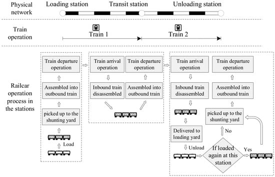
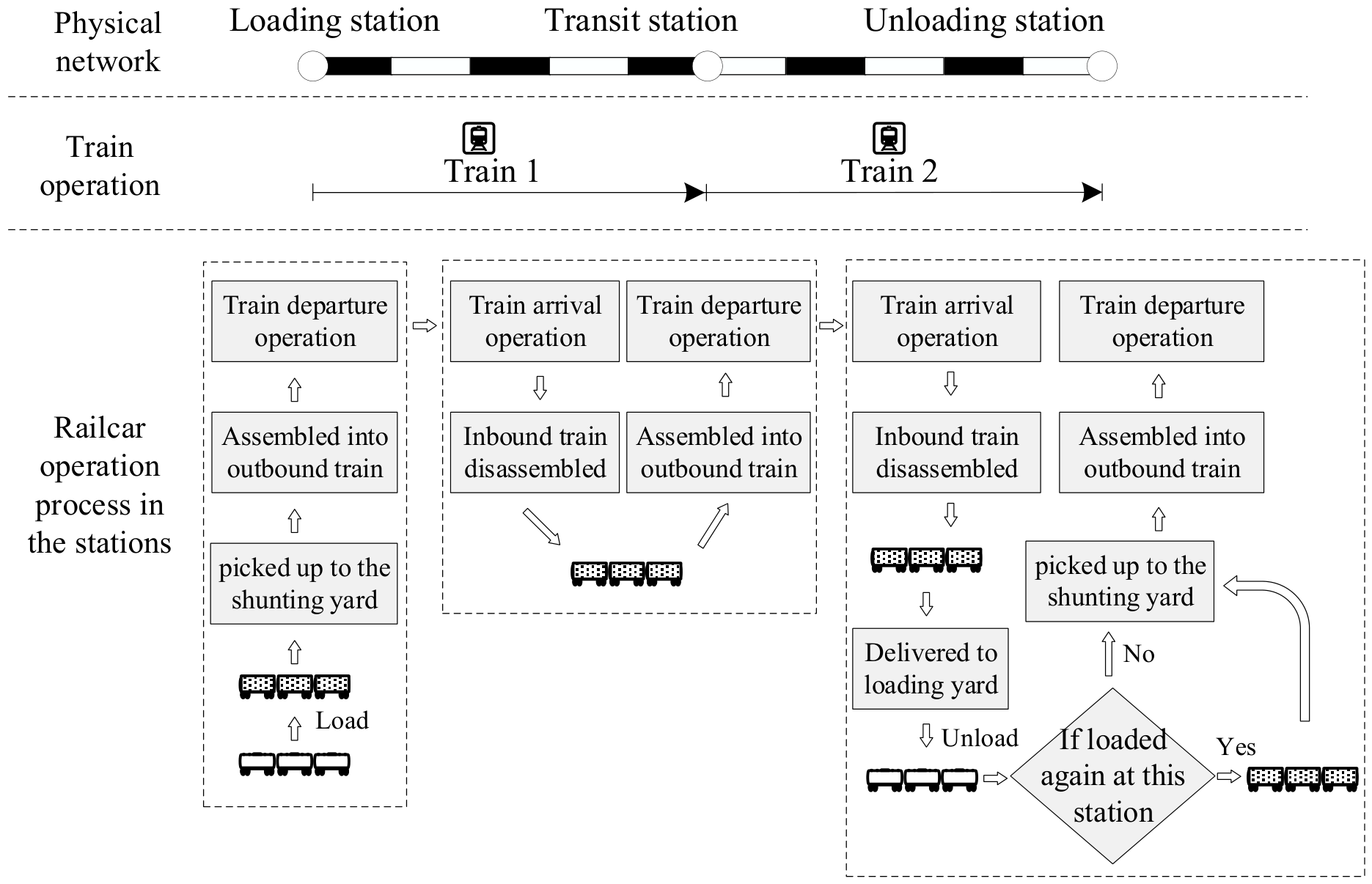
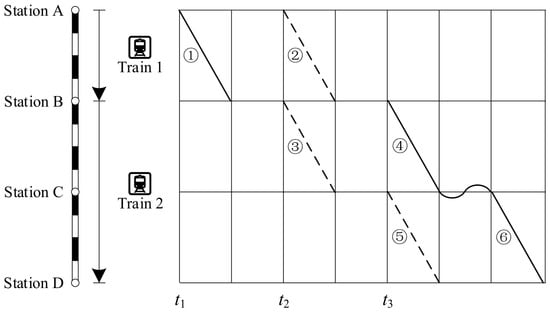
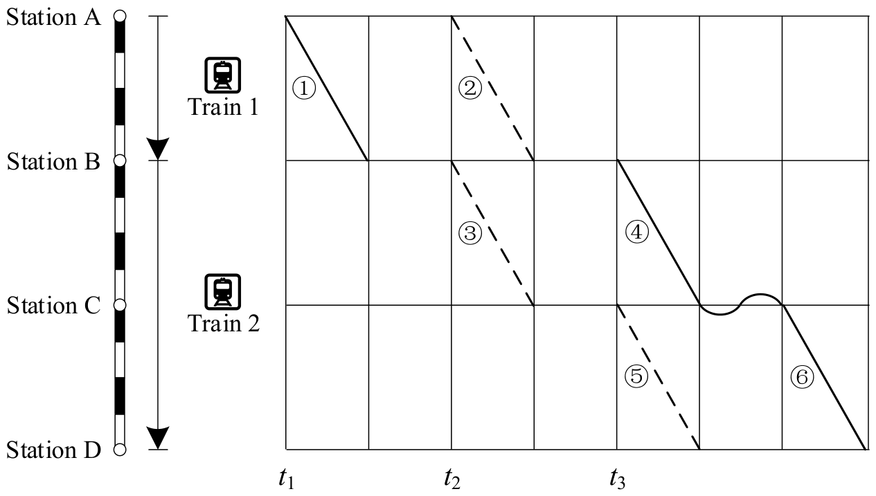
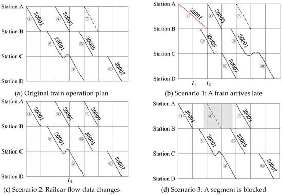
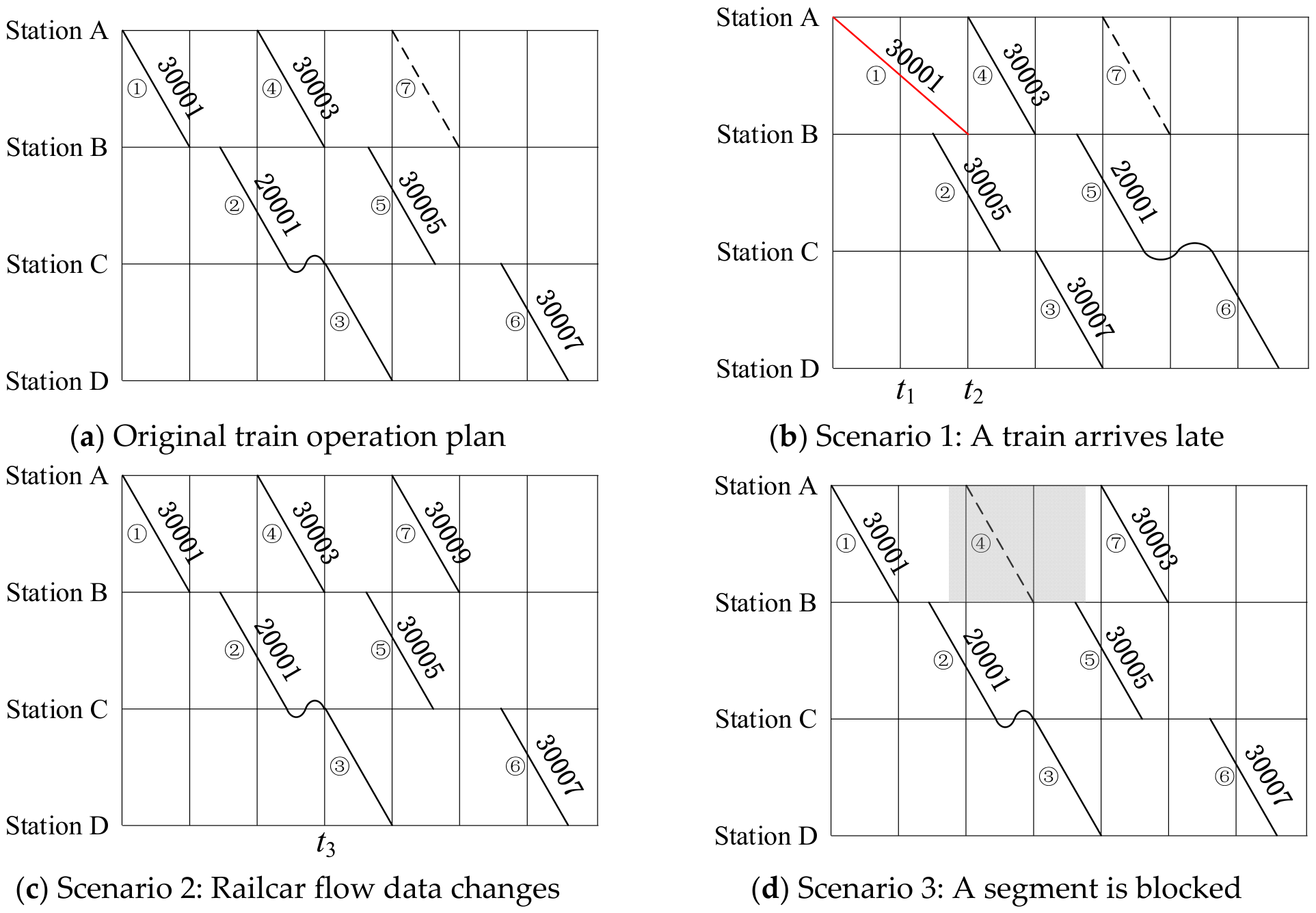
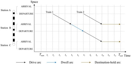
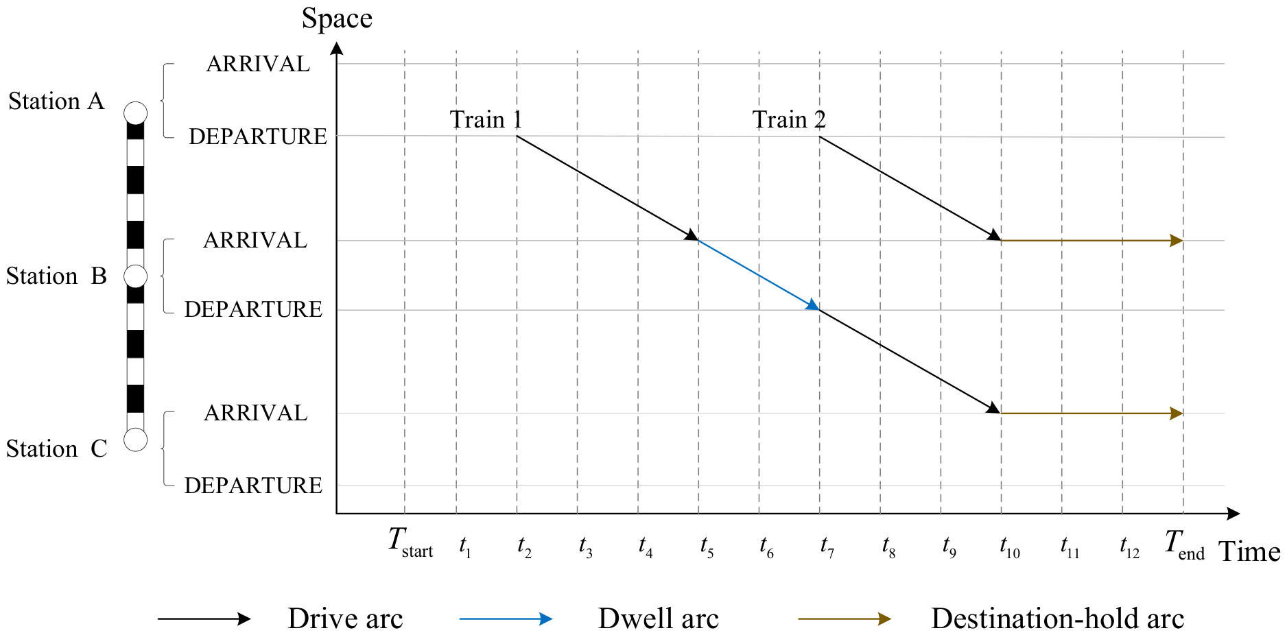
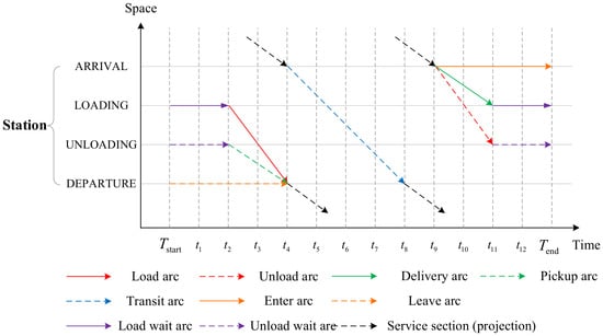
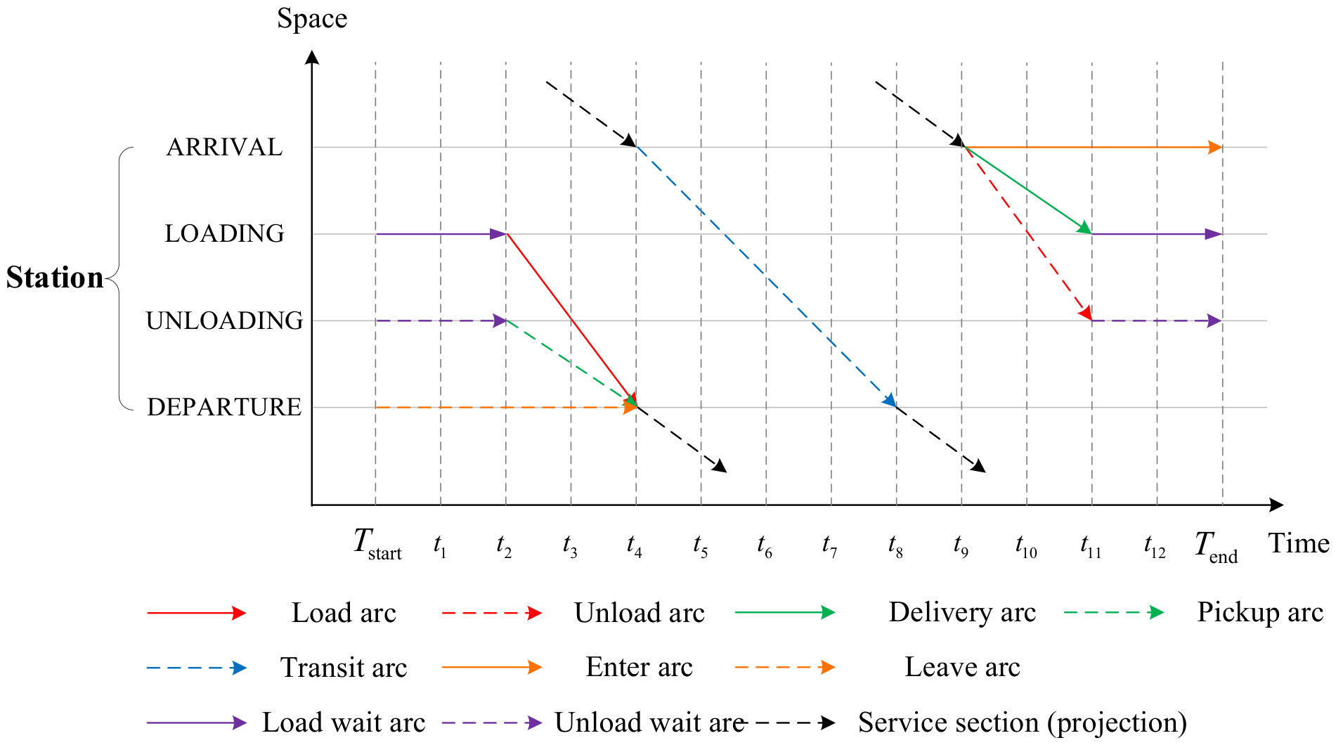
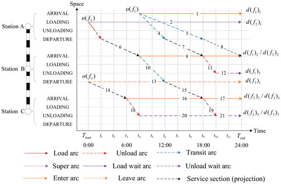
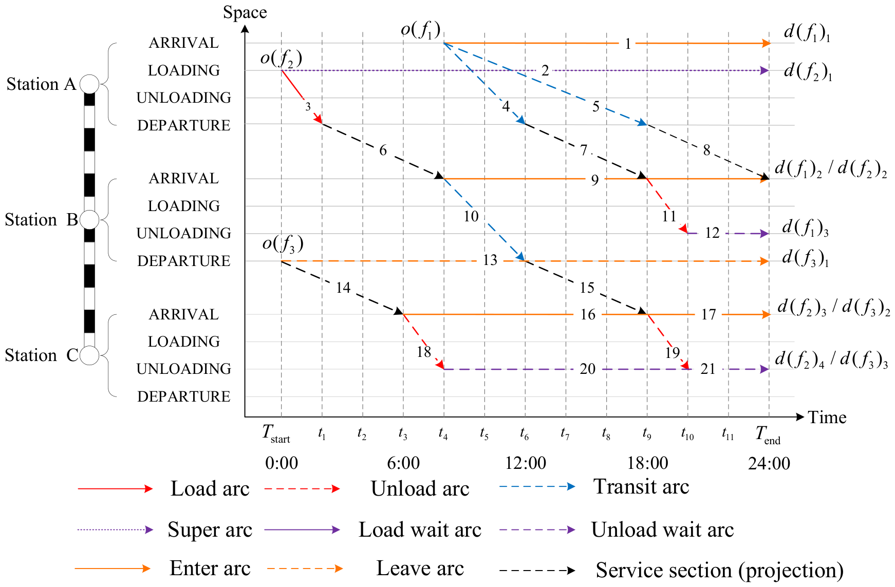
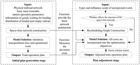
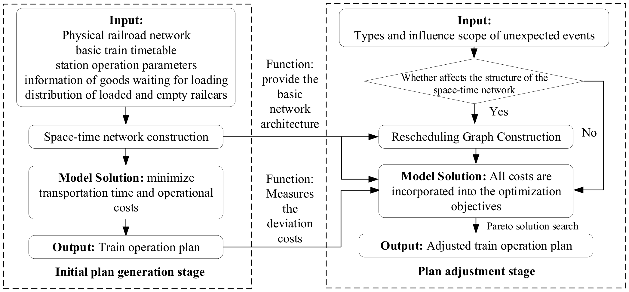
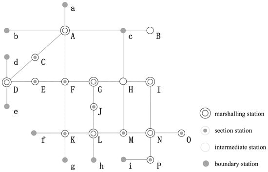
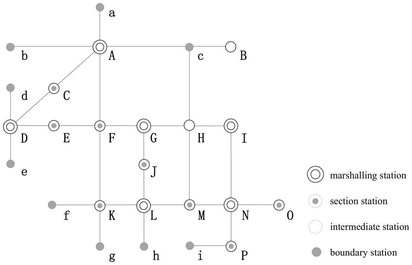
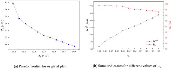
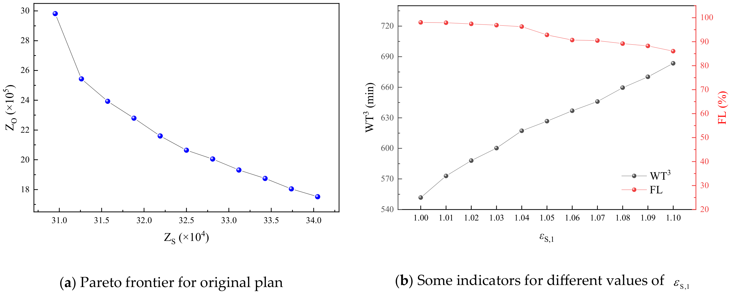
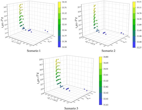
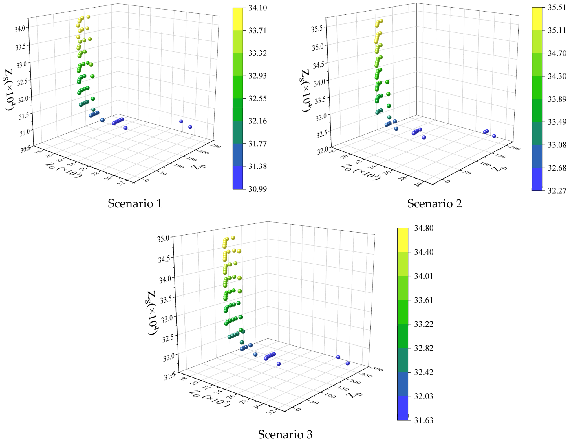
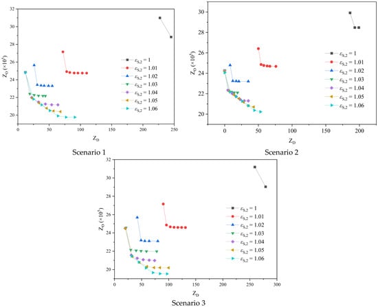
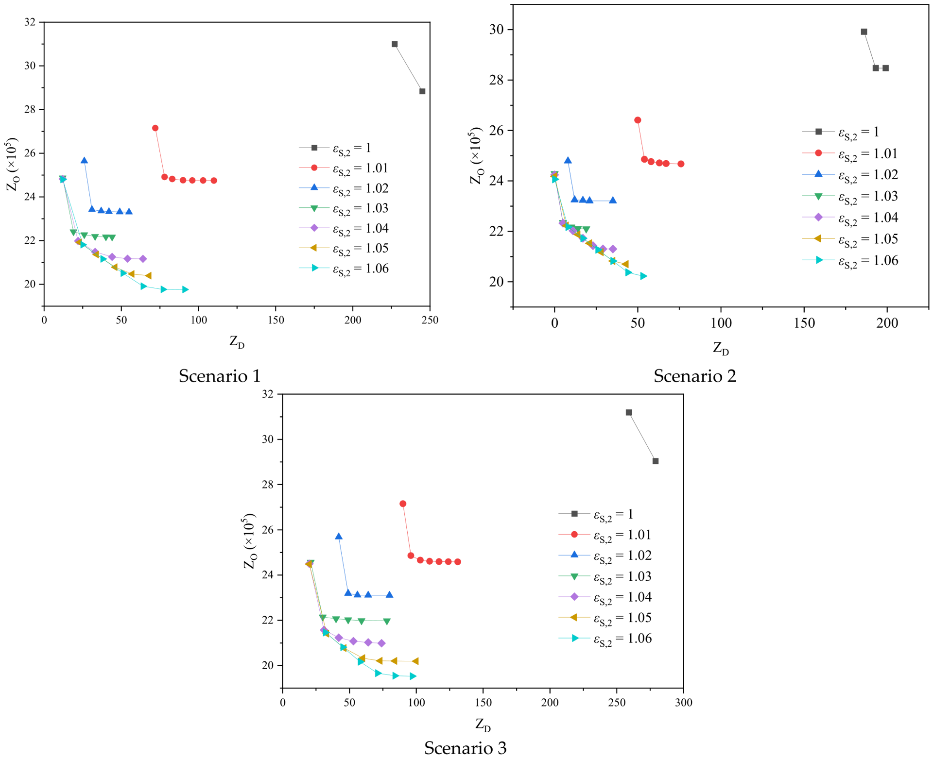
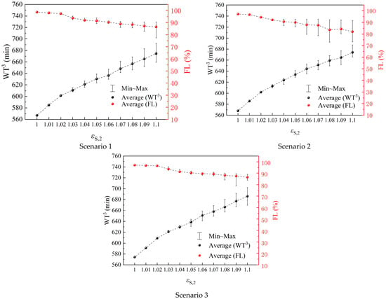
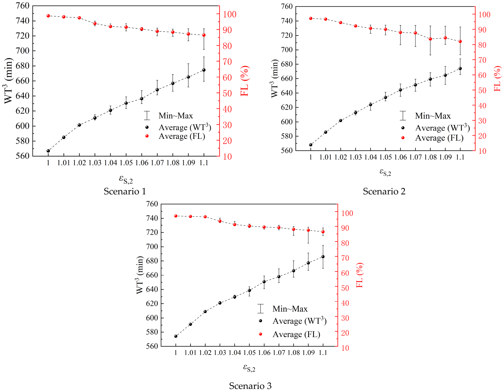
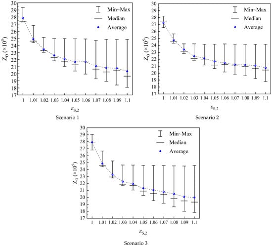
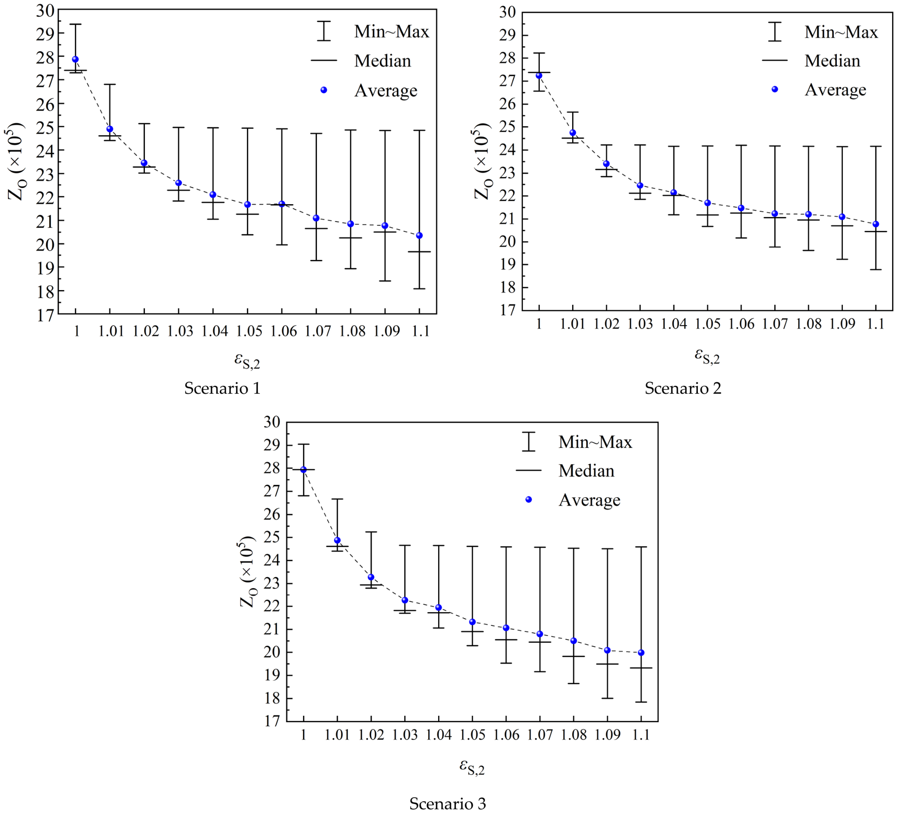
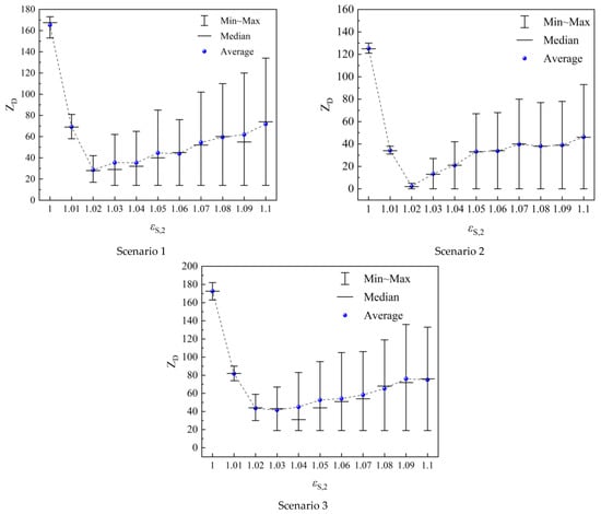
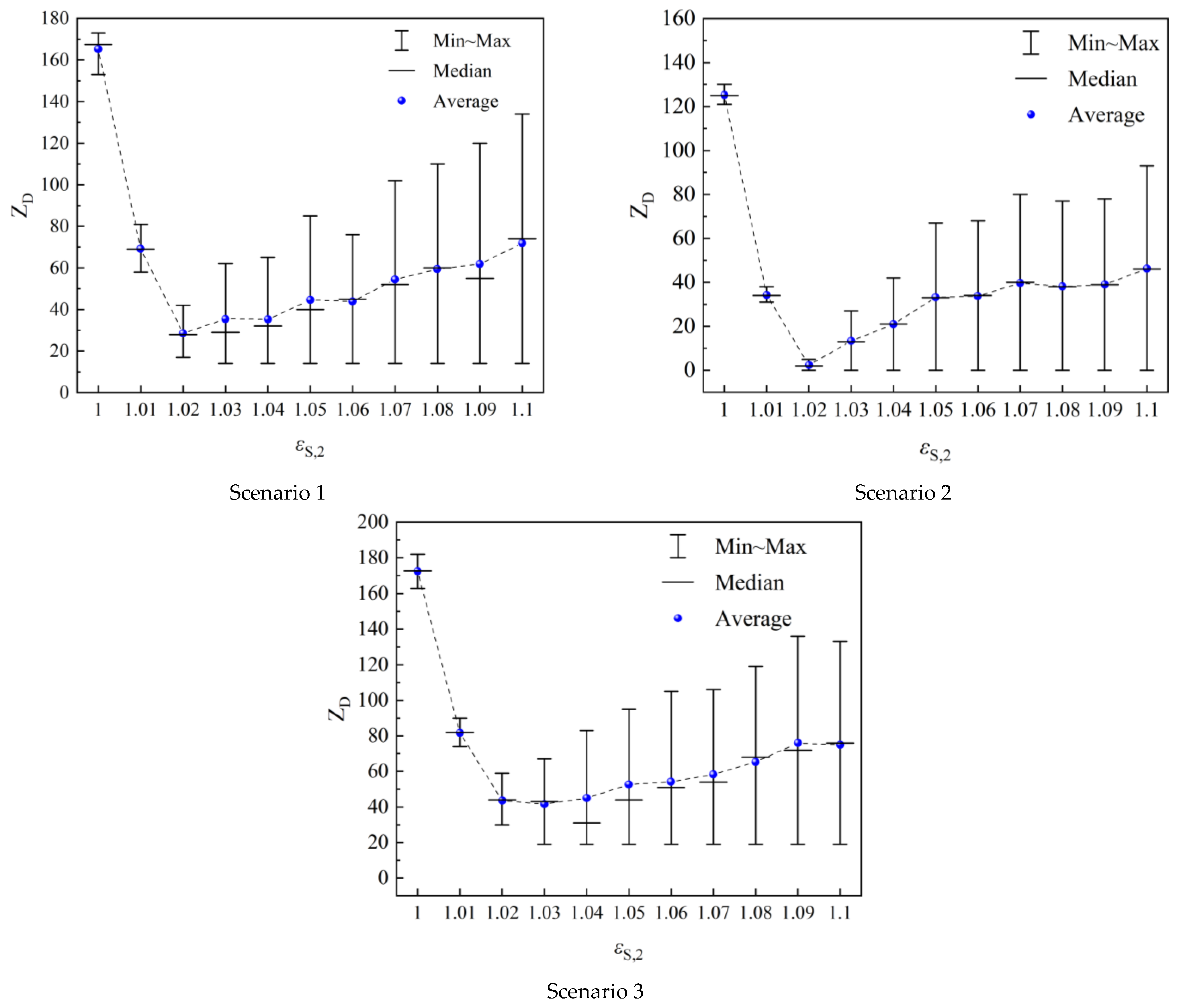
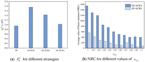
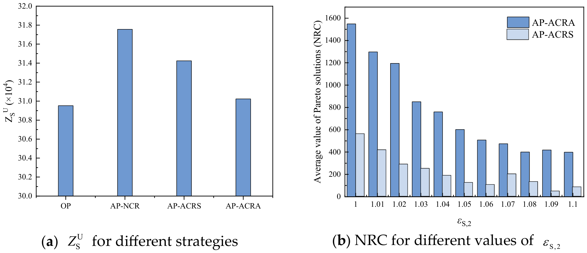
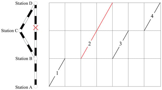
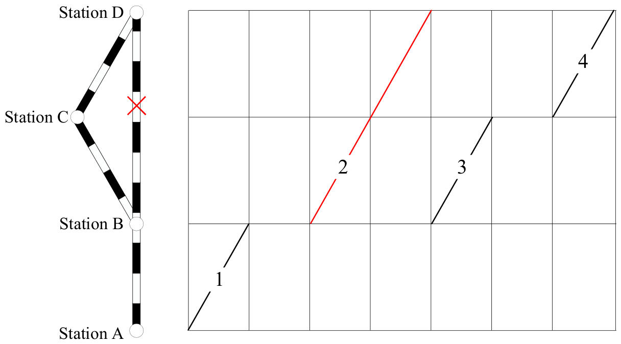
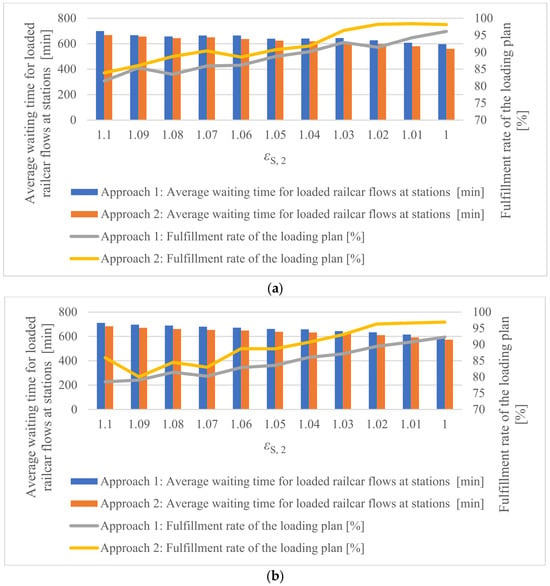
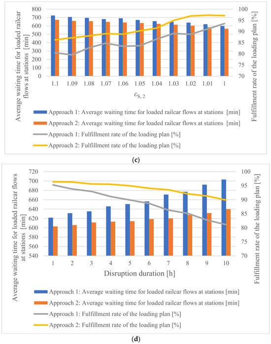
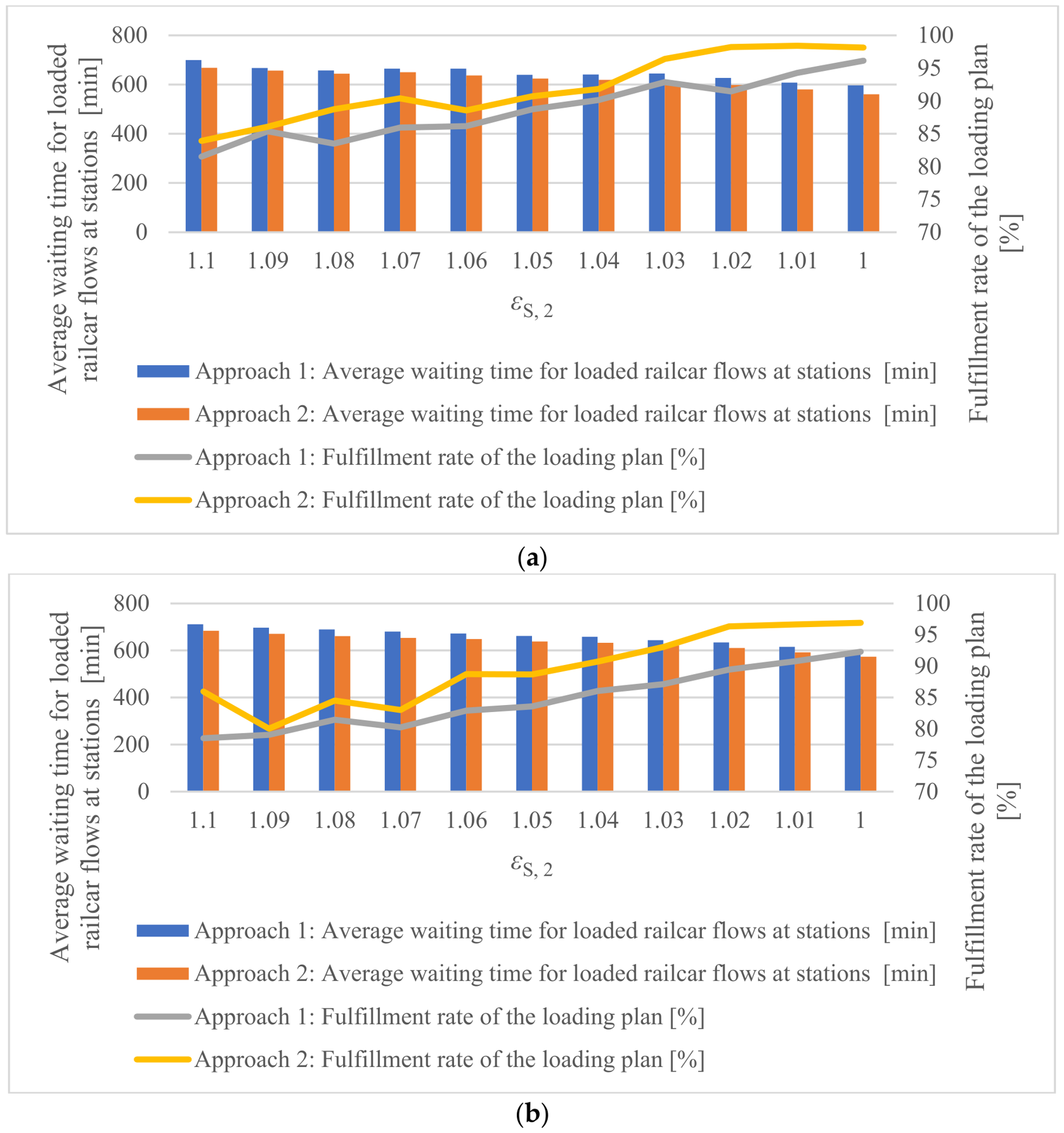
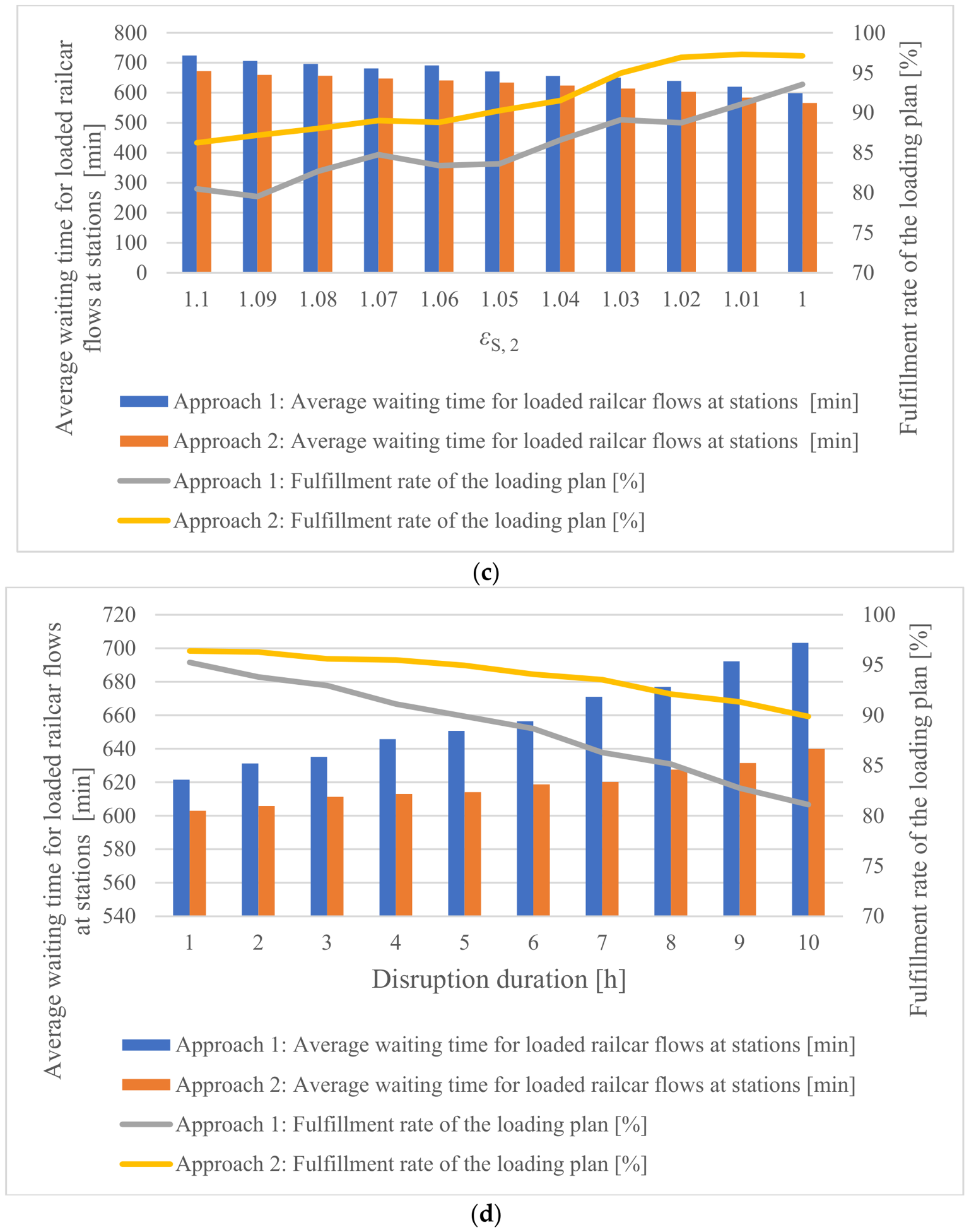
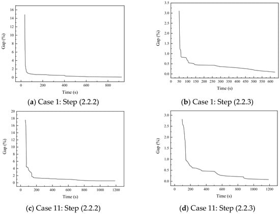
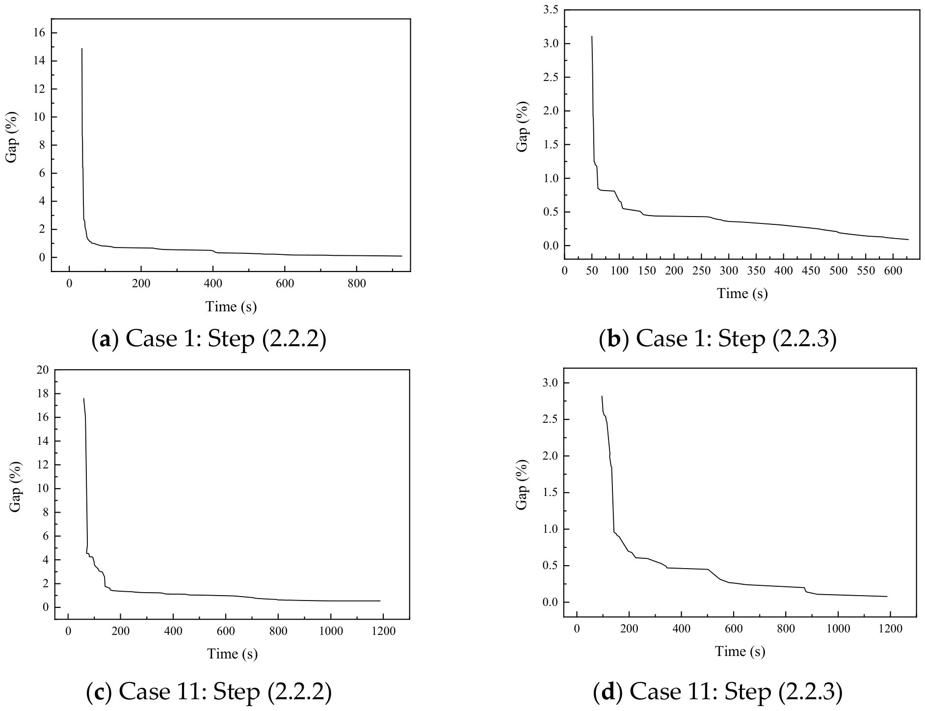

Disclaimer/Publisher’s Note: The statements, opinions and data contained in all publications are solely those of the individual author(s) and contributor(s) and not of MDPI and/or the editor(s). MDPI and/or the editor(s) disclaim responsibility for any injury to people or property resulting from any ideas, methods, instructions or products referred to in the content. |
© 2026 by the author. Licensee MDPI, Basel, Switzerland. This article is an open access article distributed under the terms and conditions of the Creative Commons Attribution (CC BY) license.