Exact Solutions to a Model for Micropolar Fluid Flows with Rayleigh Energy Dissipation

Abstract

Polynomial exact solutions of the Navier–Stokes equations for describing micropolar incompressible fluid flows with energy dissipation are reported. The transformation of mechanical energy into thermal energy is taken into account. The heat equation for the Rayleigh function contains the sum of the squares of the components of the Cauchy velocity tensor (the main component for the dissipative function). Unidirectional homogeneous and non-homogeneous fluid flows with moment stresses are considered. The solvability of overdetermined systems for studying homogeneous and non-homogeneous shear flows is studied. The paper pays attention to the exact integration of equations for three-dimensional flows. The construction of classes of exact solutions is carried out first using the Lin–Sidorov–Aristov solution family. In other words, the velocity field depends linearly on part of the coordinates. The coefficients of the linear forms of the velocity field depend on the third coordinate and time. The pressure field and the temperature field are quadratic forms with similar functional arbitrariness. In addition, exact solutions for the velocity field with a nonlinear dependence on part of the coordinates are considered.

1. Introduction

The investigation of the processes of deformation of liquids, gases and solids is generally carried out using the symmetric theory of continuum mechanics, which allows for invariant dynamic relations for the internal degrees of freedom of elementary volumes of a medium distributed in space [1,2,3,4,5,6,7,8]. In this method of describing the stress–strain state, stress tensors, strain tensors and strain rate tensors are postulated as symmetric tensors [3,4,7]. This approach is based on the motion of an elementary (representative) volume of a deformable body as a “non-local” material point performing three translational motions [1,5,7]. In other words, an elementary volume has three translational degrees of freedom [1,5,7]. The use of constitutive relations linking symmetric tensors has long been decisive in continuum physics [1,7,8].

At the beginning of the twentieth century, the Cosserat continuum was introduced into the mechanics of deformable solids [1,5,8,9]. The Cosserat continuum is a mathematical model of a continuous medium, where any elementary volume (any material point) has rotational degrees of freedom [1,5,8,9]. In other words, in Cosserat theory, each material point of a continuous medium is endowed with the properties of a solid described by six degrees of freedom (three degrees of freedom of translational motion and three degrees of freedom of rotational motion) [1,5,8,9]. In the macroworld, the simplest illustration of the motion of an elementary volume of the Cosserat continuum is the flight of a sports equipment such as a ball. Taking into account rotational degrees of freedom leads to asymmetric theories of describing the micropolar stress–strain state [1,5,8,9].

Micropolar fluids have been systematically studied in pioneering studies [10,11,12,13]. For incompressible fluids, taking into account moment stresses in the Navier–Stokes equations is equivalent to adding a new volume force. This force is expressed by a biharmonic operator proportional to the moment kinematic (dynamic) viscosity [10,11,12,13,14,15]. It is understandable that the description of micropolar fluid flows is complicated not only because of the introduction of a new force, but also because of the increase in the constants of the material medium that take into account the viscous properties [10,11,12,13,14,15]. It can be stated that at present there are no reliable methods for determining the value of the moment viscosity coefficient. As a rule, this coefficient is determined through exact solutions for unidirectional Couette–Poiseuille flows of micropolar fluids [8,10,11,12,13,16,17,18,19,20,21,22,23,24,25,26,27,28]. Thus, the problem of finding classes of exact solutions to the Navier–Stokes equations for a micropolar fluid does not lose its relevance, as for classical Newtonian fluids. Possibly, while there are no methods for determining moment viscosity, the problem of exact integration of the equations of hydrodynamics of micropolar liquids becomes even much more required for the development and construction of algorithms for exact solutions than in the case of the Navier–Stokes equations [8,16,17,18,19,20,21].

The study of the first exact solutions for describing unidirectional flows of micropolar fluids was carried out as a generalization of the classical Couette, Poiseuille, and Stokes flows for Newtonian fluids [8,16,17,18,19,20,21]. Since micropolar fluids are used in industry, an essential problem for the exact integration of the Navier–Stokes equations is the construction of exact solutions with the addition of the Rayleigh dissipative function to the entropy or heat conductivity equation [17,19,20,21,24,25,26,27,29,30].

When finding exact solutions to the Navier–Stokes equations describing the flows of classical Newtonian incompressible fluids, the transformation of mechanical energy into thermal energy (dissipative processes) is often ignored [19,20,21,29,30,31,32]. In this case, due to the absence of Benard gravitational convection and Marangoni thermocapillary convection, without taking into account the Rayleigh function, a constant temperature is assumed. This signifies that the heat conduction equation is automatically satisfied. In other words, only the trivial (constant) solution of the equation for describing the transfer of entropy or heat is considered [33,34,35,36,37,38,39,40].

Neglect of the dissipation of the kinetic energy of the flow of Newtonian and micropolar fluids into thermal energy is justified by several reasons [19,20,21,29,30,31,32]. Let us indicate two main factors that are most often used to ignore the dissipation of energy in the study of the motion of liquid (drop) media [10,11,12,13,19,20,21,29,30,31,32]. From a physics view, when considering heat transfer, the heat equation contains the Rayleigh function [10,11,12,13,19,20,21,29,30,31,32]. The coefficient in front of the sum of the squares of the tangential stresses takes values for Newtonian fluids of the order of one decimal place or less. Thus, in numerous cases this is formally assumed to be zero to simplify the equations of motion, since an assumption is naturally introduced about small enough values of the partial derivatives of velocities with respect to spatial coordinates [2,4,8,16,17,19,29,30,41,42]. For micropolar fluids, the description of energy transformation is complicated even more, since due to the asymmetry of the moment stress tensor, two moment viscosities are introduced into the Rayleigh function [10,11,12,13,19,20,21,29,30,31,32].

Ignoring the influence of the Rayleigh dissipative function from the mathematical formalism is due to the complication of the study of the qualitative and quantitative properties of the solutions of the Navier–Stokes equations [8,16,17,19,29,30,41,42,43,44]. The properties of the system of equations of motion are significantly complicated by the quadratic nonlinearity of the Rayleigh function. Thus, in analytical and numerical modeling, the convective derivative of the Navier–Stokes equations and the Joule dissipation in the heat transfer equation been compete [10,11,12,13,19,20,21,29,30,31,32].

For problems of the theory of control of Newtonian viscous incompressible fluid flows, it is to take into account the Rayleigh dissipative function [10,11,12,13,19,20,21,29,30,31,32,41,42,43,44]. Despite the closeness of the equations of fluid motion taking into account local heat release to the equations of natural convection (the Obereck–Boussinesq equations), no algorithms currently exist for finding exact solutions. Certainly, it is necessary to apply the known families of exact solutions of the Navier–Stokes equations, which were initially obtained without taking into account the dissipative function to describe the phenomena of momentum transfer in Newtonian and micropolar fluids [8,16,17,19,29,30,41,42].

The most frequently used class of exact solutions for the Navier–Stokes equations and related hydrodynamic equations are polynomial classes of exact solutions to the Navier–Stokes equations [8,16,17,19,29,30,41,42,45,46,47,48,49,50]. The first and best known family of polynomial exact solutions is the ansatz for the Lin–Sidorov–Aristov velocity field [8,16,17,19,47,48,49,50]. This family of exact solutions describes stratified fluid flows along horizontal coordinates or along a vertical variable for velocity, pressure, temperature, concentration, and other force factors [1,2,3,4,5,6,7,8,16,17,19,29,30,41,42,45,46,47,48,49,50]. The Lin–Sidorov–Aristov velocity field has been repeatedly studied and generalized [8,16,17,19,29,30,41,42,45,46,50]. Reviews of this class of exact solutions to hydrodynamic equations are contained in Refs. [8,16,17,19,29,30,41,42,45,46,50]. Modifications of this family of solutions for isobaric, gradient, convective, and thermal diffusion flows are reflected in Refs. [8,16,17,19,29,30,41,42,45,46,50]. The main observation concentrated in these scientific papers is that the linear forms of the velocity field are satisfied by a quadratic function in part of the coordinates that describes the transfer of matter, which is consistent with the pressure field. The quadratic dependence of temperature on horizontal coordinates allows us to construct exact solutions of the Navier–Stokes equations taking into account the dissipation of mechanical (kinetic) energy of a viscous incompressible fluid [16,17,19,29,30,41,42].

This paper extends the class of exact Lin–Sidorov–Aristov solutions, its generalizations and modifications for fluid flows with local heat release. We demonstarte the existence of such solutions and to determine the structure of the equation for finding the functions that determine the structure of the hydrodynamic fields of velocity, pressure and temperature. The findings point on the possibility of linearizing the equations of motion, which is realized due to the approximation of the convective derivative in the equation of fluid momentum transfer (in the Navier–Stokes equation) or in the heat transfer equation (in the heat conduction equation).

2. Equations of Motion

In what follows, we consider the unsteady flow of a micropolar viscous incompressible fluid taking into account the internal (local) heat release caused by the internal friction of the layers, which is described by the system of equations [8,10,11,12,13,14,15,16,17,19,31]:

$$\begin{gathered} {\displaystyle \frac{𝜕V}{𝜕t}}+\left(V\cdot 𝛻\right)V=-𝛻P+\nu \Delta V-\eta \Delta \Delta V, \\ {\displaystyle \frac{𝜕T}{𝜕t}}+\left(V\cdot 𝛻\right)T=\chi \Delta T+Q, \\ 𝛻\cdot V=0. \end{gathered}$$

(1)

In the system of Equation (1), consisting of the Navier–Stokes vector equation, the Fourier heat conductivity equation, and the continuity equation, the following standard notations are introduced: $V\left(t,x_1,x_2,x_3\right)=\left(V_1,V_2,V_3\right)$ is the velocity vector, a function of time (t) and space coordinates, $P$ is the pressure divided by the constant density $\rho$ is the kinematic (molecular) viscosity, $\eta$ is the moment viscosity, $\chi$ is the thermal diffusivity; $𝛻$ is the Hamilton operator, and $\Delta$ is the Laplace operator [8,16,17,19,31].

We further assume that the three-dimensional motion of the fluid is described in a rectangular Cartesian coordinate system. Thus, the Hamiltonian operator reads

$$𝛻=i_1{\displaystyle \frac{𝜕}{𝜕x}}+i_2{\displaystyle \frac{𝜕}{𝜕y}}+i_3{\displaystyle \frac{𝜕}{𝜕z}},$$

where $i_1$, $i_2$, and $i_3$ are the unit vectors of the Cartesian rectangular coordinate system. The Laplace operator and the biharmonic operator are, respectively, written as follows:

$$\Delta ={\displaystyle \frac{{𝜕}^2}{𝜕x_1^2}}+{\displaystyle \frac{{𝜕}^2}{𝜕x_2^2}}+{\displaystyle \frac{{𝜕}^2}{𝜕x_3^2}},$$

$$\Delta \Delta ={\displaystyle \frac{{𝜕}^4}{𝜕x_1^4}}+{\displaystyle \frac{{𝜕}^4}{𝜕x_2^4}}+{\displaystyle \frac{{𝜕}^4}{𝜕x_3^4}}+2\left({\displaystyle \frac{{𝜕}^4}{𝜕x_1^2𝜕x_2^2}}+{\displaystyle \frac{{𝜕}^4}{𝜕x_1^2𝜕x_3^2}}+{\displaystyle \frac{{𝜕}^4}{𝜕x_2^2𝜕x_3^2}}\right).$$

Thus, when calculating mixed derivatives, commutation of the differential operator is postulated, i.e., all derivatives are continuously differentiable up to and including the fourth order.

In the heat conductivity equation, the function Q (the Rayleigh dissipative function) determines the dissipation of fluid energy (transformation of mechanical energy into thermal energy) according to the formula [1,10,11,12,13,14,15]:

$$\begin{gathered} Q=a\left(𝛻V:{\left(𝛻V\right)}^T+𝛻V:𝛻V\right)+b\left(𝛻\omega :𝛻\omega \right)+c\left(𝛻\omega :{\left(𝛻\omega \right)}^T\right)= \\ ={\displaystyle \frac{\nu }{2c_p}}\left(V_{r,s}{V}_{r,s}+V_{r,s}{V}_{s,r}\right)+{\displaystyle \frac{2{\eta }^{\prime }}{c_p}}\left({\omega }_{r,s}{\omega }_{r,s}\right)+{\displaystyle \frac{2\eta }{c_p}}\left({\omega }_{r,s}{\omega }_{s,r}\right). \end{gathered}$$

(2)

In Equation (2), the vector $\omega ={\displaystyle \frac{1}{2}}𝛻\times V$ is the local vorticity of the fluid, which is determined by the rotational degrees of freedom for a representative volume of viscous incompressible fluid. The commas in the subscripts of the quantities denote differentiation with respect to the variable indicated after the comma. The colon denotes the convolution of tensors. In the expression (2), the Einstein rule is used, i.e., the summation of terms (expressions of partial derivatives) is carried out with respect to repeating variables. Note that for moment viscosities ${\eta }^{\prime }$ and $\eta$ the inequality is satisfied: ${\eta }^{\prime }\le \eta$ [1,10,11,12,13,14,15]. In Equation (2), the designation $c_p$ denotes the specific heat capacity of the fluid at constant pressure [31].

Note that the equations of motion (1) for describing the flow of an incompressible fluid with couple stress are based on the theory published in Ref. [51]. Vijay Stokes [10,11,12,13] adapted the couple stress theory from solid mechanics to fluid mechanics by forcing incompressibility and adding nonlinear inertia effects (Stokes wrote the equations in Euler coordinates). However, the original theory for the mechanics of deformable solids is indefinite. This problem remains in Stokes’ formulation because some stresses cannot be determined uniquely for compressible media. Although the velocity components for incompressible fluids may not be affected, stress calculations require additional assumptions and an additional fluid parameter. Furthermore, a true couple stress continuum should not simply ignore independent pairs of bodies. These problems were later resolved in Refs. [16,17,18,32,44,45], which developed a consistent system for fluid mechanics with skew-symmetric couple stresses for compressible and incompressible media. Note that the system (1) coincides for incompressible media with the equations given in Ref. [51].

The difference between micropolar fluids and classical Newtonian fluids is the appearance of additional moment viscosity in the Rayleigh dissipative function. This is explained by the asymmetry of the moment stress tensor. Currently, there is increasing interest in studying the nonlinear properties of the Navier–Stokes equations for describing the flows of Newtonian and micropolar fluids with Rayleigh energy dissipation. For kinematic and moment viscosity, there is a quantitative estimate of the order of dissipative coefficients [10,11,12,13,14,15]:

$${\displaystyle \frac{\nu }{\eta }}~{\displaystyle \frac{10^{-6}}{10^{-10}}} >> 1.$$

(3)

According to the simplest estimate (3) and following qualitative studies of the properties of solutions of hydrodynamic equations with dissipation [16,17,19,30,31,41,42], we further consider function (2) in the form

$$Q={\displaystyle \frac{\nu }{2c_p}}{{\sum }_{i=1}^3{\sum }_{j=1}^3\left({\displaystyle \frac{𝜕V_i}{𝜕x_j}}+{\displaystyle \frac{𝜕V_j}{𝜕x_i}}\right)}^2.$$

(4)

By transforming and summing the expressions in brackets for the Rayleigh function (4), one obtains its representation in the following form:

$$\begin{gathered} Q=\nu \left[2{\left({\displaystyle \frac{𝜕V_1}{𝜕x_1}}\right)}^2+2{\left({\displaystyle \frac{𝜕V_2}{𝜕x_2}}\right)}^2+2{\left({\displaystyle \frac{𝜕V_3}{𝜕x_3}}\right)}^2+{\left({\displaystyle \frac{𝜕V_1}{𝜕x_2}}\right)}^2+{\left({\displaystyle \frac{𝜕V_2}{𝜕x_1}}\right)}^2+{\left({\displaystyle \frac{𝜕V_1}{𝜕x_3}}\right)}^2\right. \\ \left. +{\left({\displaystyle \frac{𝜕V_3}{𝜕x_1}}\right)}^2+{\left({\displaystyle \frac{𝜕V_2}{𝜕x_3}}\right)}^2+{\left({\displaystyle \frac{𝜕V_3}{𝜕x_2}}\right)}^2+2\left({\displaystyle \frac{𝜕V_1}{𝜕x_2}}\right)\left({\displaystyle \frac{𝜕V_2}{𝜕x_1}}\right)+2\left({\displaystyle \frac{𝜕V_1}{𝜕x_3}}\right)\left({\displaystyle \frac{𝜕V_3}{𝜕x_1}}\right)+2\left({\displaystyle \frac{𝜕V_2}{𝜕x_3}}\right)\left({\displaystyle \frac{𝜕V_3}{𝜕x_2}}\right)\right]. \end{gathered}$$

(5)

In scalar forms, the system (1) with the substitution of the dissipative function in the form (5) reads

$$\begin{gathered} {\displaystyle \frac{𝜕V_1}{𝜕t}}+V_1{\displaystyle \frac{𝜕V_1}{𝜕x_1}}+V_2{\displaystyle \frac{𝜕V_1}{𝜕x_2}}+V_3{\displaystyle \frac{𝜕V_1}{𝜕x_3}}=-{\displaystyle \frac{𝜕P}{𝜕x_1}}+\nu \left({\displaystyle \frac{{𝜕}^2{V}_1}{𝜕x_1^2}}+{\displaystyle \frac{{𝜕}^2{V}_1}{𝜕x_2^2}}+{\displaystyle \frac{{𝜕}^2{V}_1}{𝜕x_3^2}}\right) \\ -\eta \left({\displaystyle \frac{{𝜕}^4{V}_1}{𝜕x_1^4}}+{\displaystyle \frac{{𝜕}^4{V}_1}{𝜕x_2^4}}+{\displaystyle \frac{{𝜕}^4{V}_1}{𝜕x_3^4}}+2\left({\displaystyle \frac{{𝜕}^4{V}_1}{𝜕x_1^2𝜕x_2^2}}+{\displaystyle \frac{{𝜕}^4{V}_1}{𝜕x_1^2𝜕x_3^2}}+{\displaystyle \frac{{𝜕}^4{V}_1}{𝜕x_2^2𝜕x_3^2}}\right)\right), \\ \hspace{1em}\hspace{1em}\hspace{1em}\hspace{1em}\hspace{1em}\hspace{1em}\hspace{1em}{\displaystyle \frac{𝜕V_2}{𝜕t}}+V_1{\displaystyle \frac{𝜕V_2}{𝜕x_1}}+V_2{\displaystyle \frac{𝜕V_2}{𝜕x_2}}+V_3{\displaystyle \frac{𝜕V_2}{𝜕x_3}}=-{\displaystyle \frac{𝜕P}{𝜕x_2}}+\nu \left({\displaystyle \frac{{𝜕}^2{V}_2}{𝜕x_1^2}}+{\displaystyle \frac{{𝜕}^2{V}_2}{𝜕x_2^2}}+{\displaystyle \frac{{𝜕}^2{V}_2}{𝜕x_3^2}}\right) \\ -\eta \left({\displaystyle \frac{{𝜕}^4{V}_2}{𝜕x_1^4}}+{\displaystyle \frac{{𝜕}^4{V}_2}{𝜕x_2^4}}+{\displaystyle \frac{{𝜕}^4{V}_2}{𝜕x_3^4}}+2\left({\displaystyle \frac{{𝜕}^4{V}_2}{𝜕x_1^2𝜕x_2^2}}+{\displaystyle \frac{{𝜕}^4{V}_2}{𝜕x_1^2𝜕x_3^2}}+{\displaystyle \frac{{𝜕}^4{V}_2}{𝜕x_2^2𝜕x_3^2}}\right)\right), \\ {\displaystyle \frac{𝜕V_3}{𝜕t}}+V_1{\displaystyle \frac{𝜕V_3}{𝜕x_1}}+V_2{\displaystyle \frac{𝜕V_3}{𝜕x_2}}+V_3{\displaystyle \frac{𝜕V_3}{𝜕x_3}}=-{\displaystyle \frac{𝜕P}{𝜕x_3}}+\nu \left({\displaystyle \frac{{𝜕}^2{V}_3}{𝜕x_1^2}}+{\displaystyle \frac{{𝜕}^2{V}_3}{𝜕x_2^2}}+{\displaystyle \frac{{𝜕}^2{V}_3}{𝜕x_3^2}}\right) \\ -\eta \left({\displaystyle \frac{{𝜕}^4{V}_3}{𝜕x_1^4}}+{\displaystyle \frac{{𝜕}^4{V}_3}{𝜕x_2^4}}+{\displaystyle \frac{{𝜕}^4{V}_3}{𝜕x_3^4}}+2\left({\displaystyle \frac{{𝜕}^4{V}_3}{𝜕x_1^2𝜕x_2^2}}+{\displaystyle \frac{{𝜕}^4{V}_3}{𝜕x_1^2𝜕x_3^2}}+{\displaystyle \frac{{𝜕}^4{V}_3}{𝜕x_2^2𝜕x_3^2}}\right)\right), \\ {\displaystyle \frac{𝜕T}{𝜕t}}+V_1{\displaystyle \frac{𝜕T}{𝜕x_1}}+V_2{\displaystyle \frac{𝜕T}{𝜕x_2}}+V_3{\displaystyle \frac{𝜕T}{𝜕x_3}}=\chi \left({\displaystyle \frac{{𝜕}^{2}T}{𝜕x_1^2}}+{\displaystyle \frac{{𝜕}^{2}T}{𝜕x_2^2}}+{\displaystyle \frac{{𝜕}^{2}T}{𝜕x_3^2}}\right) \\ +{\displaystyle \frac{\nu }{c_p}}\left[2{\left({\displaystyle \frac{𝜕V_1}{𝜕x_1}}\right)}^2+2{\left({\displaystyle \frac{𝜕V_2}{𝜕x_2}}\right)}^2+2{\left({\displaystyle \frac{𝜕V_3}{𝜕x_3}}\right)}^2+{\left({\displaystyle \frac{𝜕V_1}{𝜕x_2}}\right)}^2+{\left({\displaystyle \frac{𝜕V_2}{𝜕x_1}}\right)}^2+{\left({\displaystyle \frac{𝜕V_1}{𝜕x_3}}\right)}^2+{\left({\displaystyle \frac{𝜕V_3}{𝜕x_1}}\right)}^2+{\left({\displaystyle \frac{𝜕V_2}{𝜕x_3}}\right)}^2+{\left({\displaystyle \frac{𝜕V_3}{𝜕x_2}}\right)}^2\right. \\ \left.+2\left({\displaystyle \frac{𝜕V_1}{𝜕x_2}}\right)\left({\displaystyle \frac{𝜕V_2}{𝜕x_1}}\right)+2\left({\displaystyle \frac{𝜕V_1}{𝜕x_3}}\right)\left({\displaystyle \frac{𝜕V_3}{𝜕x_1}}\right)+2\left({\displaystyle \frac{𝜕V_2}{𝜕x_3}}\right)\left({\displaystyle \frac{𝜕V_3}{𝜕x_2}}\right)\right], \\ {\displaystyle \frac{𝜕V_1}{𝜕x_1}}+{\displaystyle \frac{𝜕V_2}{𝜕x_2}}+{\displaystyle \frac{𝜕V_3}{𝜕x_3}}=0. \end{gathered}$$

(6)

For the system of Equation (6), several families of exact solutions are obtained in the polynomial class of velocities, linearly and nonlinearly dependent with respect to part of the coordinates [8,16,17,19,29,30,41,42,45,46,47,48,49,50]. These solutions are based on the use of two classes of exact solutions. The first class represents a family with a velocity field linearly dependent on two spatial coordinates (the Lin–Sidorov–Aristov class) [47,48,49,50]. The second class represents a family of solutions with a velocity field nonlinearly dependent on two spatial coordinates [29,30,41,42].

3. Unidirectional Flows

Let us now consider a special case for the system of Equation (6). The traditional presentation of the theoretical foundations of hydrodynamics begins with the consideration of unidirectional flows (one component of the velocity vector is not equal to zero). For unidirectional flows of Newtonian and micropolar fluids, a homogeneous layered flow with a Couette–Poiseuille profile is considered [8]:

$$\mathit{V}=\left({\mathit{V}}_{\mathbf{1}}\left(\mathit{t},{\mathit{x}}_{\mathbf{3}}\right),\mathbf{0},\mathbf{0}\right).$$

The Couette–Poiseuille velocity profile $V=\left(V_1\left(t,x_3\right),\mathrm{0,0}\right)$ in this case depends on the transverse coordinate $x_3$ and time $t$. The function $V_1\left(t,x_3\right)$ satisfies the simplest linear parabolic inhomogeneous partial differential equation for a Newtonian fluid [1,2,3,4,5,6,7,8,16,17,19]:

$${\displaystyle \frac{𝜕V_1}{𝜕t}}=-{\displaystyle \frac{𝜕P}{𝜕x_1}}+\nu {\displaystyle \frac{{𝜕}^2{V}_1}{𝜕x_3^2}}.$$

Recall that the horizontal pressure gradient for the Poiseuille flow is a number, i.e., it takes a constant value throughout the entire fluid flow region, or a function that depends on time. In Refs. [1,2,3,4,5,6,7,8,16,17,19], it was shown that the Couette–Poiseuille profile satisfies the equation [8,19]

$${\displaystyle \frac{𝜕V_1}{𝜕t}}=-{\displaystyle \frac{𝜕P}{𝜕x_1}}+\nu {\displaystyle \frac{{𝜕}^2{V}_1}{𝜕x_3^2}}-\eta {\displaystyle \frac{{𝜕}^4{V}_1}{𝜕x_3^4}}$$

to describe micropolar fluids. In [8,19], it was shown that the classical homogeneous Couette–Poiseuille profile can be generalized to study non-uniform unidirectional flows of a micropolar fluid. Below, we briefly present an algorithm for constructing exact solutions with spatial non-uniformity of the velocity profile of a unidirectional flow.

We represent the velocity vector of a moving micropolar fluid as follows:

$$V=\left(V_1\left(t,x_1,x_2,x_3\right),0,0\right).$$

(7)

Therefore, we assume that the flow velocity changes in several directions [8,16,17,19,20,21], that is, the velocity field (7) describes non-uniform unidirectional flows of a micropolar viscous incompressible fluid. To determine the unknown component of vector (7), it must be substituted into the system of Equation (6). Note that from the incompressibility equation included in the system (6) for vector field (7), the differential relation follows

$${\displaystyle \frac{𝜕V_1}{𝜕x_1}}=0.$$

Understandably, the solution to the last equation is a functional dependence on two spatial coordinates and time:

$$V_1=V_1\left(t,x_2,x_3\right).$$

(8)

We further substitute expression (8) into the system of Equation (6), and obtain the following equations for determining the speed, pressure and temperature:

$$\begin{gathered} {\displaystyle \frac{𝜕V_1}{𝜕t}}=-{\displaystyle \frac{𝜕P}{𝜕x_1}}+\nu \left({\displaystyle \frac{{𝜕}^2{V}_1}{𝜕x_2^2}}+{\displaystyle \frac{{𝜕}^2{V}_1}{𝜕x_3^2}}\right)-\eta \left({\displaystyle \frac{{𝜕}^4{V}_1}{𝜕x_2^4}}+{\displaystyle \frac{{𝜕}^4{V}_1}{𝜕x_3^4}}+2{\displaystyle \frac{{𝜕}^4{V}_1}{𝜕x_2^2𝜕x_3^2}}\right), \\ {\displaystyle \frac{𝜕P}{𝜕x_2}}=0,{\displaystyle \frac{𝜕P}{𝜕x_3}}=0, \\ {\displaystyle \frac{𝜕T}{𝜕t}}+V_1{\displaystyle \frac{𝜕T}{𝜕x_1}}=\chi \left({\displaystyle \frac{{𝜕}^{2}T}{𝜕x_1^2}}+{\displaystyle \frac{{𝜕}^{2}T}{𝜕x_2^2}}+{\displaystyle \frac{{𝜕}^{2}T}{𝜕x_3^2}}\right)+{\displaystyle \frac{\nu }{c_p}}\left[{\left({\displaystyle \frac{𝜕V_1}{𝜕x_2}}\right)}^2+{\left({\displaystyle \frac{𝜕V_1}{𝜕x_3}}\right)}^2\right], \end{gathered}$$

(9)

respectively.

The system of Equation (9) is weakly coupled. It consists of two subsystems. From the system (9) and the form of the exact solution (10), one can first determine the flow velocity, and then calculate the exact solution for the temperature. Thus, it is instructive to first write out the exact solutions for the velocity field and for the pressure field.

We indicate several classes of exact solutions for the system of equations. Note that the pressure normalized to a constant density is described by a linear form with coefficients over time t:

$$P=P_0\left(t\right)+P_1\left(t\right)x_1.$$

(10)

For the pressure field (10), which describes a non-uniform gradient flow of a micropolar fluid, the exact solution for the velocity field is described by the formula

$$V_1=U\left(x_3,t\right)+x_2{u}_1\left(x_3,t\right).$$

(11)

The exact solution (11) is a superposition of the classical Couette–Poiseuille profile $U\left(x_3,t\right)$ and the non-uniform term $u_1\left(x_3,t\right)$, which is the spatial velocity gradient. Consequently, the expression for the velocity field (11) can be attributed to the class of exact solutions obtained by additive and multiplicative separation of variables (a polynomial exact solution with a functional choice of coefficients in the expressions for the monomials) [8,16,17]. Reasoning further in a similar way, one can obtain the following representation of the velocity vector for a non-uniform unidirectional flow of a micropolar fluid:

$$V_1=U\left(x_3,t\right)+{\sum }_{k=1}^N{\displaystyle \frac{x_2^k}{k!}}{u}_k\left(x_3,t\right),$$

(12)

where N is a natural number.

Let us give an example of the equations for determining unknown functions if in Equation (12) $N=2$ is set. Thus, for the speed the exact solution has the form:

$$V_1=U\left(x_3,t\right)+x_2{u}_1\left(x_3,t\right)+{\displaystyle \frac{x_2^2}{2}}{u}_2\left(x_3,t\right),$$

To determine the unknown functions in the exact solution (11) or (12) after calculating the corresponding partial derivatives

$$\begin{gathered} {\displaystyle \frac{𝜕V_1}{𝜕t}}={\displaystyle \frac{𝜕U}{𝜕t}}+x_2{\displaystyle \frac{𝜕u_1}{𝜕t}}+{\displaystyle \frac{x_2^2}{2}}{\displaystyle \frac{𝜕u_2}{𝜕t}},{\displaystyle \frac{{𝜕}^4{V}_1}{𝜕x_2^4}}=u_2, \\ {\displaystyle \frac{{𝜕}^4{V}_1}{𝜕x_2^2𝜕x_3^2}}={\displaystyle \frac{{𝜕}^4{u}_2}{𝜕x_3^2}},{\displaystyle \frac{{𝜕}^4{V}_1}{𝜕x_3^4}}={\displaystyle \frac{{𝜕}^{4}U}{𝜕x_3^4}}+y{\displaystyle \frac{{𝜕}^4{u}_1}{𝜕x_3^4}}+{\displaystyle \frac{y^2}{2}}{\displaystyle \frac{{𝜕}^4{u}_2}{𝜕x_3^4}}, \end{gathered}$$

it is necessary to substitute the expressions (10)–(12) into the system (9):

$$\begin{gathered} {\displaystyle \frac{𝜕U}{𝜕t}}+x_2{\displaystyle \frac{𝜕u_1}{𝜕t}}+{\displaystyle \frac{x_2^2}{2}}{\displaystyle \frac{𝜕u_2}{𝜕t}}=\nu \left(u_2+{\displaystyle \frac{{𝜕}^{2}U}{𝜕x_3^2}}+y{\displaystyle \frac{{𝜕}^2{u}_1}{𝜕x_3^2}}+{\displaystyle \frac{y^2}{2}}{\displaystyle \frac{{𝜕}^2{u}_2}{𝜕x_3^2}}\right)- \\ -\eta \left({\displaystyle \frac{{𝜕}^4{u}_2}{𝜕x_3^2}}+{\displaystyle \frac{{𝜕}^{4}U}{𝜕x_3^4}}+y{\displaystyle \frac{{𝜕}^4{u}_1}{𝜕x_3^4}}+{\displaystyle \frac{y^2}{2}}{\displaystyle \frac{{𝜕}^4{u}_2}{𝜕x_3^4}}\right). \end{gathered}$$

Applying the method of undetermined coefficients to the last equation, one obtains a system consisting of linear coupled partial differential equations:

$$\begin{gathered} {\displaystyle \frac{𝜕U}{𝜕t}}=\nu \left(u_2+{\displaystyle \frac{{𝜕}^{2}U}{𝜕x_3^2}}\right)-\eta \left({\displaystyle \frac{{𝜕}^4{u}_2}{𝜕x_3^2}}+{\displaystyle \frac{{𝜕}^{4}U}{𝜕x_3^4}}\right), \\ {\displaystyle \frac{𝜕u_1}{𝜕t}}=\nu {\displaystyle \frac{{𝜕}^2{u}_1}{𝜕x_3^2}}-\eta {\displaystyle \frac{{𝜕}^4{u}_1}{𝜕x_3^4}}, \\ {\displaystyle \frac{𝜕u_2}{𝜕t}}=\nu {\displaystyle \frac{{𝜕}^2{u}_2}{𝜕x_3^2}}-\eta {\displaystyle \frac{{𝜕}^4{u}_2}{𝜕x_3^4}}. \end{gathered}$$

(13)

The equation for the velocity $U\left(x_3,t\right)$ contains the function $u_2\left(x_3,t\right)$. It determines the heterogeneity of the partial differential equation. Thus, if, in the exact solution, it is necessary to consider terms with a nonlinear dependence. on the coordinate $x_2$ (monomials $x_2^k$, where $k\ge 2$), then the obtained exact solution is not a superposition of terms (12):

$$U\left(x_3,t\right),x_2{u}_1\left(x_3,t\right), \dots ,{\displaystyle \frac{x_2^N}{N!}}{u}_2\left(x_3,t\right).$$

Exact polynomial solutions for the velocity (8), similar to expressions (12), were obtained in Refs. [8,29,30,40,41].

The temperature field, if r the exact solution (1) is considered, has the following polynomial representation:

$$T=T_0\left(x_3,t\right)+T_1\left(x_3,t\right)x_1+T_2\left(x_3,t\right)x_2+T_{11}\left(x_3,t\right){\displaystyle \frac{x_1^2}{2}}+T_{12}\left(x_3,t\right)x_1{x}_2+T_{22}\left(x_3,t\right){\displaystyle \frac{x_2^2}{2}}.$$

(14)

The unknown functions of the temperature field are determined similarly to obtaining system (13). Repeating this technique, one obtains equations for determining the functions of the temperature field:

$$\begin{gathered} {\displaystyle \frac{𝜕T_1}{𝜕t}}=\chi {\displaystyle \frac{{𝜕}^2{T}_1}{𝜕x_3^2}},{\displaystyle \frac{𝜕T_2}{𝜕t}}=\chi {\displaystyle \frac{{𝜕}^2{T}_2}{𝜕x_3^2}}, \\ {\displaystyle \frac{𝜕T_{11}}{𝜕t}}=\chi {\displaystyle \frac{{𝜕}^2{T}_{11}}{𝜕x_3^2}},{\displaystyle \frac{𝜕T_{12}}{𝜕t}}=\chi {\displaystyle \frac{{𝜕}^2{T}_{12}}{𝜕x_3^2}},{\displaystyle \frac{𝜕T_{22}}{𝜕t}}=\chi {\displaystyle \frac{{𝜕}^2{T}_{22}}{𝜕x_3^2}}, \\ {\displaystyle \frac{𝜕T_0}{𝜕t}}+U{T}_1=\chi {\displaystyle \frac{{𝜕}^2{T}_0}{𝜕x_3^2}}+\chi \left(T_{11}+T_{22}\right)+{\displaystyle \frac{2\nu }{c_p}}{\left({\displaystyle \frac{𝜕U}{𝜕x_3}}\right)}^2. \end{gathered}$$

(15)

The system of Equation (15) consists of five quite simple linear homogeneous parabolic heat conduction equations and one non-homogeneous equation. The structure of Equation (15) allows us to construct a generalization of the exact solution (14) for the velocity field (1), linear with respect to one horizontal (longitudinal) coordinate. The polynomial representation for temperature has the form:

$$T=T_0\left(x_3,t\right)+T_1\left(x_3,t\right)x_1+{\sum }_{k=1}^M{\displaystyle \frac{x_2^k}{k!}}{T}_{k+2}\left(x_3,t\right).$$

(16)

Here, $M$ is a natural number independent of the number from the Formula (12).

If the velocity field (12) with a nonlinear dependence on the horizontal coordinate is considered, then the expression for the temperature is determined by Formula (16), but the inequality $M\ge 2N$ has to be satisfied. This inequality allows balancing the terms of the temperature field with the terms of the velocity field.

We demonstrate the difference between exact solutions of the Navier–Stokes equations with energy dissipation for micropolar fluids and Newtonian fluids. We consider a flow under a constant horizontal pressure gradient with velocity profile $V_1=U\left(x_3\right)$ in an infinite layer of liquid with thickness $h$. To describe the flows of micropolar fluids, it is necessary to formulate more boundary conditions than for Newtonian fluids [9,10,11,12,13,14,15,16]. This must be done because of the higher order of the differential equations describing the steady-state flow of micropolar fluids.

4. Boundary Value Problem for Unidirectional Flow

Recall that for the classical Navier–Stokes equations, the order of differential equations for describing steady and unsteady flows with respect to spatial ones is determined by the Laplace operator. Thus, the Navier–Stokes equations for describing a Newtonian viscous incompressible fluid are of the second order. If fluid flows with couple stresses are considered, then the order of the equations is determined by the biharmonic operator. Thus, the order of the Navier–Stokes equations for describing fluid flows with couple stresses (micropolar fluids) is equal to four. Due to the increase in the order of differential equations for the hydrodynamics of micropolar fluids, the boundary conditions for describing steady flows reported in Refs. [10,11,12,13,14,15] are used below in this section.

To illustrate the exact solution, let us consider a unidirectional steady-state Poiseuille flow of a micropolar fluid with energy dissipation (${\displaystyle \frac{𝜕P}{𝜕x_1}}=\mathrm{c}\mathrm{o}\mathrm{n}\mathrm{s}\mathrm{t}=A$). The steady-state flow is described by a system of ordinary differential equations:

$$\begin{gathered} \eta {\displaystyle \frac{{𝜕}^4{V}_1}{𝜕x_3^4}}-\nu {\displaystyle \frac{{𝜕}^2{V}_1}{𝜕x_3^2}}=-A, \\ \chi {\displaystyle \frac{{𝜕}^{2}T}{𝜕x_3^2}}=-{\displaystyle \frac{\nu }{c_p}}{\left({\displaystyle \frac{𝜕V_1}{𝜕x_3}}\right)}^2, \end{gathered}$$

The general solution of this linear system of ordinary differential equations in quasi-polynomials is written as

$$\begin{gathered} V_1={\displaystyle \frac{\eta }{\nu }}\left(C_1\exp \left(x_3\sqrt{{\displaystyle \frac{\nu }{\eta }}}\right)+C_2\exp \left(-x_3\sqrt{{\displaystyle \frac{\nu }{\eta }}}\right)\right)+{\displaystyle \frac{A{x}_3^2}{2\nu }}+C_3+x_3{C}_4, \\ T={\displaystyle \frac{2{\eta }^{3/2}}{c_p{\nu }^2\chi }}\left(\exp \left(x_3\sqrt{{\displaystyle \frac{\nu }{\eta }}}\right)C_1\left(2A{\eta }^{1/2}-Az{\nu }^{1/2}-{\nu }^{3/2}{C}_4\right)+\right. \\ +\left.\exp \left(-x_3\sqrt{{\displaystyle \frac{\nu }{\eta }}}\right)C_2\left(2A{\eta }^{1/2}+Az{\nu }^{1/2}+{\nu }^{3/2}{C}_4\right)\right)- \\ -{\displaystyle \frac{1}{4c_p\nu \chi }}\left(\exp \left(2x_3\sqrt{{\displaystyle \frac{\nu }{\eta }}}\right){\eta }^2{C}_1^2+\exp \left(-2x_3\sqrt{{\displaystyle \frac{\nu }{\eta }}}\right){\eta }^2{C}_2^2\right)- \\ -{\displaystyle \frac{A^2{x}_3^4+4A{x}_3^3\nu C_4+6x_3^2\nu \left(\nu C_4^2-2\eta C_1{C}_2\right)}{12c_p\nu \chi }}+C_5+x_3{C}_6. \end{gathered}$$

Hereafter, the solutions obtained in this paper, are verified by direct substitution into differential equations. Note that in this case, the solution satisfies the general nonlinear system (6).

We consider two boundary-value problems [10,11,12,13,14,15]:

$$\begin{gathered} (\mathrm{I}){\left.{\displaystyle \frac{dU}{d{x}_3}}\right|}_{x_3=0}={\left.{\displaystyle \frac{dU}{d{x}_3}}\right|}_{x_3=h}=0,U\left(0\right)=U\left(h\right)=0; \\ (\mathrm{II}){\left.{\displaystyle \frac{d^{2}U}{d{x}_3^2}}\right|}_{z=0}={\left.{\displaystyle \frac{d^{2}U}{d{x}_3^2}}\right|}_{z=h}=0,U\left(0\right)=U\left(h\right)=0. \end{gathered}$$

For both boundary value problems, the no-slip condition is satisfied (the velocities at the boundaries of the liquid layer are equal to zero). For the first boundary-value problem, zero moment stresses [10,11,12,13,14,15,31]

$${\left.{\displaystyle \frac{dU}{d{x}_3}}\right|}_{x_3=0}={\left.{\displaystyle \frac{dU}{d{x}_3}}\right|}_{x_3=h}=0$$

are specified at the layer boundaries; for the second boundary-value problem, the condition of zero vorticity [10,11,12,13,14,15,31],

$${\left.{\displaystyle \frac{d^{2}U}{d{x}_3^2}}\right|}_{x_3=0}={\left.{\displaystyle \frac{d^{2}U}{d{x}_3^2}}\right|}_{x_3=h}=0,$$

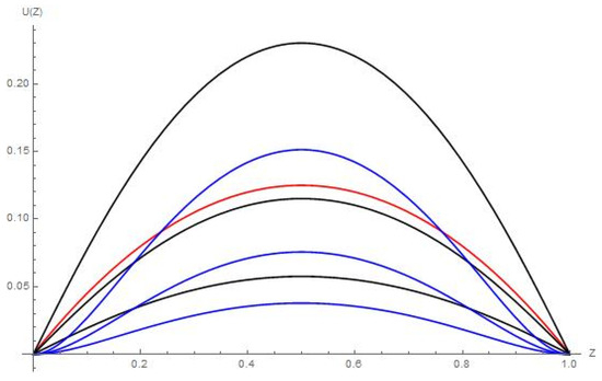
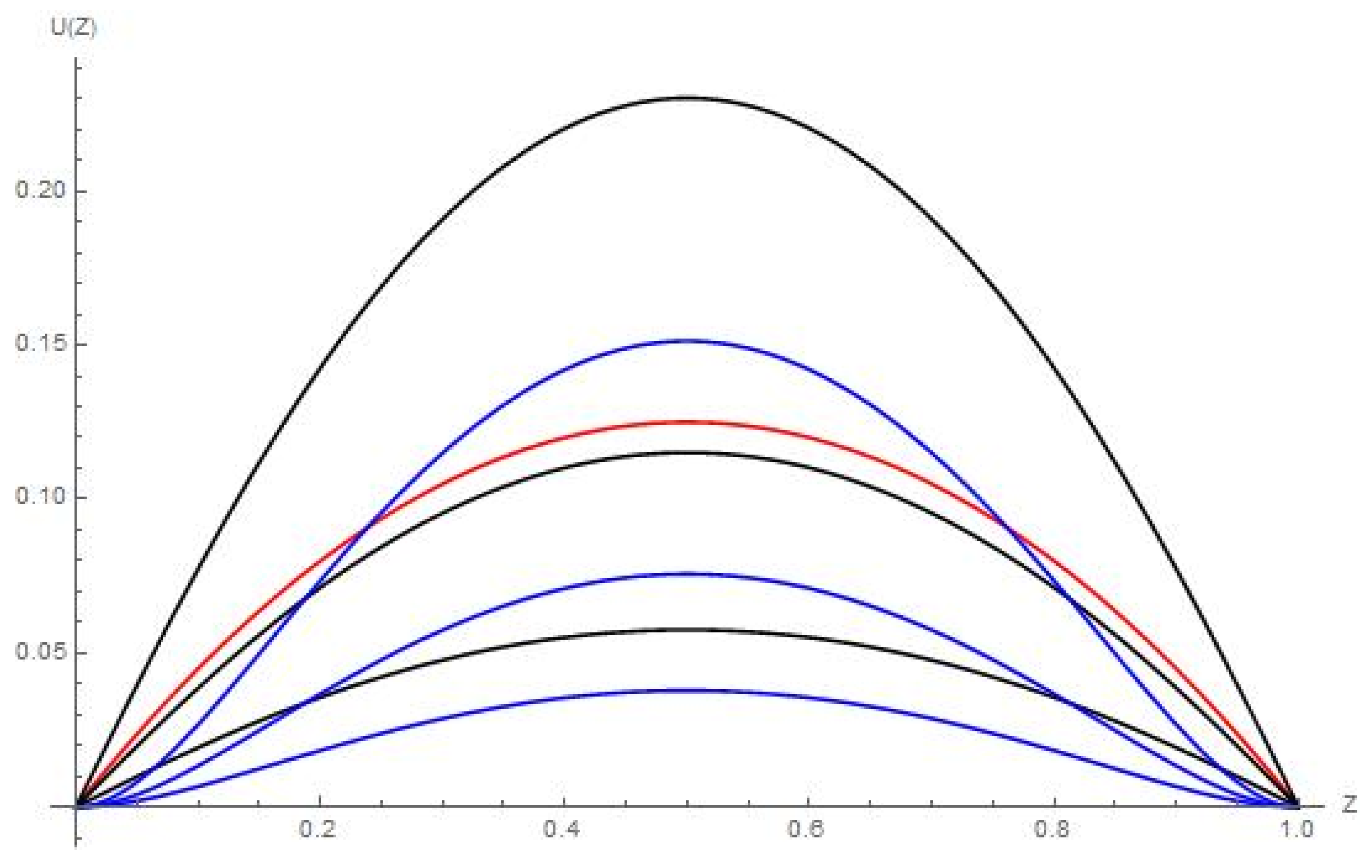
at the layer boundaries is used. Figure 1 shows velocity profiles illustrating solutions the two boundary-value problems.

Figure 1. Fluid velocity profiles for the first and second boundary-value problems: the red line shows the classical fluid, the black line shows the flow of micropolar fluid for boundary-value problem I, the blue line shows the flow of micropolar fluid for boundary-value problem II. See text for details.

The boundary conditions used in this study are classical [1,5,8,10,12,17]. They are used to illustrate the novelty of the exact solution. The exact solutions obtained can be used for new types of boundary conditions reported in Refs. [19,20,27,29,30], but is a separate study beyond this paper.

In Figure 1, the velocity profiles are presented for the same values of the Reynolds number (the parameter characterizing the Newtonian effects of the fluid) and for a constant value of the pressure gradient. It is understandable that the velocity profile changes relative to both boundary value-problems if the parameter of moment (couple) stresses is varied. This signifies that for fluids with couple stresses it is possible to regulate the fluid flow rate over the cross section of the channel. Note that the obtained profiles are consistent with the studies published in Refs. [1,9,10,11,12,13,14,15,31].

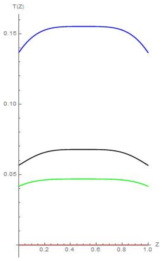
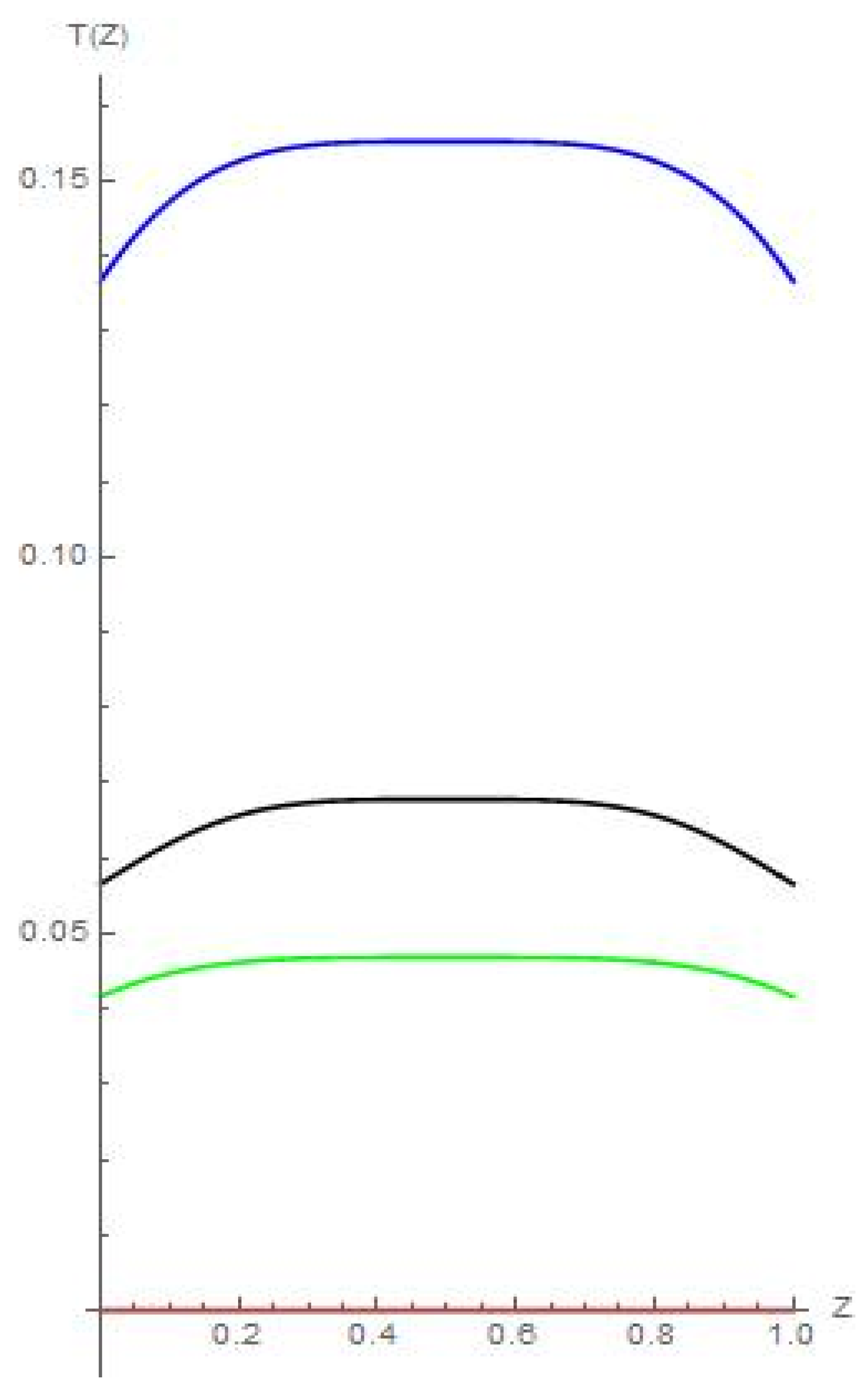
If moment stresses are taken into account when describing liquids, then with a fixed pressure gradient it becomes possible to control the flow and its consumption. This is the main difference from a Newtonian liquid with translational degrees of freedom. The ability to vary the velocity profile of the liquid and the use of energy dissipation allows us to study the change in temperature for a moving liquid (Figure 2).

Figure 2. Temperature profiles for the first and second boundary-value problems: red line—isothermal flow, green line—classical fluid, black line—micropolar fluid flow for boundary value-problem I, blue line—micropolar fluid flow for boundary-value problem II.

The temperature profiles shown in Figure 2 illustrate not only the importance of the rheological characteristics of the fluid, but also the conditions at the flow boundary. The choice of boundary conditions requires each time additional physical justification and the design of technical devices with possible “switching” of boundary conditions during operation. The construction of exact solutions for simple regions in which steady-state unidirectional fluid flow can be realized demonstrates the need to obtain new governing equations and boundary conditions for modeling and simulating flows of complex fluids. The study of temperature profiles allows us to conclude that taking into account the transformation of energy in liquids allows better heat removal from heated elements by a flow of micropolar liquids.

Figure 1 and Figure 2 are given for the only Reynolds number $\mathrm{Re}=10$ and illustrate the importance of choosing the type of coolant and the method for treating the surfaces over which the fluid flows. The resulting precise solutions allows quite simple physical experiments to select coatings that implements complex three-dimensional flows [20,21].

5. Three-Dimensional Fluid Flows

Let us proceed to the study of three-dimensional flows of micropolar viscous incompressible fluids. We construct an exact solution to the nonlinear system of partial differential Equation (6) and consider a velocity field with a linear dependence on two spatial coordinates [8,29,30,40,41]. In other words, we use the first family of polynomial exact Lin–Sidorov–Aristov solutions [16,17,19,47,48,49,50]. Let us represent the velocity field for a three-dimensional velocity vector as follows:

$$\begin{gathered} V_1=U\left(x_3,t\right)+U_1\left(x_3,t\right)x_1+U_2\left(x_3,t\right)x_2, \\ {V}_2=W\left(x_3,t\right)+W_1\left(x_3,t\right)x_1+W_2\left(x_3,t\right)x_2, \\ {V}_3=w\left(x_3,t\right). \end{gathered}$$

(17)

Expressions (4) for the velocities are linear forms relative to the horizontal (longitudinal) coordinates $x_1$ and $x_2$ with coefficients U, U₁, U₂, W, W₁, W₂, and w, depending on the vertical (transverse) coordinate $x_3$ and time $t$. The pressure and temperature field are described by quadratic forms:

$$\begin{gathered} P=P_0\left(x_3,t\right)+P_1\left(x_3,t\right)x_1+P_2\left(x_3,t\right)x_2 \\ +P_{11}\left(x_3,t\right){\displaystyle \frac{x_1^2}{2}}+P_{12}\left(x_3,t\right)x_1{x}_2+P_{22}\left(x_3,t\right){\displaystyle \frac{x_2^2}{2}}, \\ T=T_0\left(x_3,t\right)+T_1\left(x_3,t\right)x_1+T_2\left(x_3,t\right)x_2+ \\ +T_{11}\left(x_3,t\right){\displaystyle \frac{x_1^2}{2}}+T_{12}\left(x_3,t\right)x_1{x}_2+T_{22}\left(x_3,t\right){\displaystyle \frac{x_2^2}{2}}. \end{gathered}$$

(18)

To analyze and study the properties of fluid flows, it is necessary to calculate the coefficients of forms (17) and (18). Let us calculate the partial derivatives of functions with respect to spatial coordinates and time, describing the velocity field (17) and the pressure and temperature fields (18):

$$\begin{gathered} {\displaystyle \frac{𝜕V_1}{𝜕t}}={\displaystyle \frac{𝜕U}{𝜕t}}+{\displaystyle \frac{𝜕U_1}{𝜕t}}{x}_1+{\displaystyle \frac{𝜕U_2}{𝜕t}}{x}_2, \\ {\displaystyle \frac{𝜕V_1}{𝜕x_1}}=U_1,{\displaystyle \frac{𝜕V_1}{𝜕x_2}}=U_2, \\ {\displaystyle \frac{𝜕V_1}{𝜕x_3}}={\displaystyle \frac{𝜕U}{𝜕x_3}}+{\displaystyle \frac{𝜕U_1}{𝜕x_3}}{x}_1+{\displaystyle \frac{𝜕U_2}{𝜕x_3}}{x}_2, \\ {\displaystyle \frac{𝜕P}{𝜕x_1}}=P_1+P_{11}{x}_1+P_{12}{x}_2,{\displaystyle \frac{𝜕P}{𝜕x_2}}=P_2+P_{12}{x}_1+P_{22}{x}_2, \\ {\displaystyle \frac{𝜕P}{𝜕x_3}}={\displaystyle \frac{𝜕P_0}{𝜕x_3}}+{\displaystyle \frac{𝜕P_1}{𝜕x_3}}{x}_1+{\displaystyle \frac{𝜕P_2}{𝜕x_3}}{x}_2+{\displaystyle \frac{𝜕P_{11}}{𝜕x_3}}{\displaystyle \frac{x_1^2}{2}}+{\displaystyle \frac{𝜕P_{12}}{𝜕x_3}}{x}_1{x}_2+{\displaystyle \frac{𝜕P_{22}}{𝜕x_3}}{\displaystyle \frac{x_2^2}{2}}, \\ {\displaystyle \frac{{𝜕}^2{V}_1}{𝜕x_1^2}}=0,{\displaystyle \frac{{𝜕}^2{V}_1}{𝜕x_2^2}}=0,{\displaystyle \frac{{𝜕}^2{V}_1}{𝜕x_3^2}}={\displaystyle \frac{{𝜕}^{2}U}{𝜕x_3^2}}+{\displaystyle \frac{{𝜕}^2{U}_1}{𝜕x_3^2}}{x}_1+{\displaystyle \frac{{𝜕}^2{U}_2}{𝜕x_3^2}}{x}_2, \\ {\displaystyle \frac{𝜕V_2}{𝜕t}}={\displaystyle \frac{𝜕W}{𝜕t}}+{\displaystyle \frac{𝜕W_1}{𝜕t}}{x}_1+{\displaystyle \frac{𝜕W_2}{𝜕t}}{x}_2, \\ {\displaystyle \frac{𝜕V_2}{𝜕x_1}}=W_1,{\displaystyle \frac{𝜕V_2}{𝜕x_2}}=W_2, \\ {\displaystyle \frac{𝜕V_2}{𝜕x_3}}={\displaystyle \frac{𝜕W}{𝜕x_3}}+{\displaystyle \frac{𝜕W_1}{𝜕x_3}}{x}_1+{\displaystyle \frac{𝜕W_2}{𝜕x_3}}{x}_2, \\ {\displaystyle \frac{{𝜕}^2{V}_2}{𝜕x_1^2}}=0,{\displaystyle \frac{{𝜕}^2{V}_2}{𝜕x_2^2}}=0,{\displaystyle \frac{{𝜕}^2{V}_2}{𝜕x_3^2}}={\displaystyle \frac{{𝜕}^{2}W}{𝜕x_3^2}}+{\displaystyle \frac{{𝜕}^2{W}_1}{𝜕x_3^2}}{x}_1+{\displaystyle \frac{{𝜕}^2{W}_2}{𝜕x_3^2}}{x}_2, \\ {\displaystyle \frac{𝜕V_3}{𝜕t}}={\displaystyle \frac{𝜕w}{𝜕t}},{\displaystyle \frac{𝜕V_3}{𝜕x_3}}={\displaystyle \frac{𝜕w}{𝜕x_3}},{\displaystyle \frac{𝜕V_3}{𝜕x_1}}=0,{\displaystyle \frac{𝜕V_3}{𝜕x_2}}=0,{\displaystyle \frac{{𝜕}^2{V}_3}{𝜕x_1^2}}=0,{\displaystyle \frac{{𝜕}^2{V}_3}{𝜕x_2^2}}=0,{\displaystyle \frac{{𝜕}^2{V}_3}{𝜕x_3^2}}={\displaystyle \frac{{𝜕}^{2}w}{𝜕x_3^2}}, \\ {\displaystyle \frac{{𝜕}^4{V}_1}{𝜕x_1^4}}=0,{\displaystyle \frac{{𝜕}^4{V}_1}{𝜕x_2^4}}=0,{\displaystyle \frac{{𝜕}^4{V}_1}{𝜕x_1^2𝜕x_2^2}}=0,{\displaystyle \frac{{𝜕}^4{V}_1}{𝜕x_1^2𝜕x_3^2}}=0,{\displaystyle \frac{{𝜕}^4{V}_1}{𝜕x_2^2𝜕x_3^2}}0, \\ {\displaystyle \frac{{𝜕}^4{V}_2}{𝜕x_1^4}}=0,{\displaystyle \frac{{𝜕}^4{V}_2}{𝜕x_2^4}}=0,{\displaystyle \frac{{𝜕}^4{V}_2}{𝜕x_1^2𝜕x_2^2}}=0,{\displaystyle \frac{{𝜕}^4{V}_2}{𝜕x_1^2𝜕x_3^2}}=0,{\displaystyle \frac{{𝜕}^4{V}_2}{𝜕x_2^2𝜕x_3^2}}0,{\displaystyle \frac{{𝜕}^4{V}_3}{𝜕x_1^4}}=0,{\displaystyle \frac{{𝜕}^4{V}_3}{𝜕x_2^4}}=0, \\ {\displaystyle \frac{{𝜕}^4{V}_3}{𝜕x_1^2𝜕x_2^2}}=0,{\displaystyle \frac{{𝜕}^4{V}_3}{𝜕x_1^2𝜕x_3^2}}=0,{\displaystyle \frac{{𝜕}^4{V}_3}{𝜕x_2^2𝜕x_3^2}}0,{\displaystyle \frac{{𝜕}^4{V}_1}{𝜕x_3^4}}={\displaystyle \frac{{𝜕}^{4}U}{𝜕x_3^4}}+{\displaystyle \frac{{𝜕}^4{U}_1}{𝜕x_3^4}}{x}_1+{\displaystyle \frac{{𝜕}^4{U}_2}{𝜕x_3^4}}{x}_2, \\ {\displaystyle \frac{{𝜕}^4{V}_2}{𝜕x_3^4}}={\displaystyle \frac{{𝜕}^{4}W}{𝜕x_3^4}}+{\displaystyle \frac{{𝜕}^4{W}_1}{𝜕x_3^4}}{x}_1+{\displaystyle \frac{{𝜕}^4{W}_2}{𝜕x_3^4}}{x}_2,{\displaystyle \frac{{𝜕}^4{V}_3}{𝜕x_3^4}}={\displaystyle \frac{{𝜕}^{4}w}{𝜕x_3^4}}, \\ {\displaystyle \frac{𝜕T}{𝜕t}}={\displaystyle \frac{𝜕T_0}{𝜕t}}+{\displaystyle \frac{𝜕T_1}{𝜕t}}{x}_1+{\displaystyle \frac{𝜕T_2}{𝜕t}}{x}_2+{\displaystyle \frac{𝜕T_{11}}{𝜕t}}{\displaystyle \frac{x_1^2}{2}}+{\displaystyle \frac{𝜕T_{12}}{𝜕t}}{x}_1{x}_2+{\displaystyle \frac{𝜕T_{22}}{𝜕t}}{\displaystyle \frac{x_2^2}{2}}, \\ {\displaystyle \frac{𝜕T}{𝜕x_1}}=T_1+T_{11}{x}_1+T_{12}{x}_2,{\displaystyle \frac{𝜕T}{𝜕x_2}}=T_2+T_{12}{x}_1+T_{22}{x}_2, \\ {\displaystyle \frac{𝜕T}{𝜕x_3}}={\displaystyle \frac{𝜕T_0}{𝜕x_3}}+{\displaystyle \frac{𝜕T_1}{𝜕x_3}}{x}_1+{\displaystyle \frac{𝜕T_2}{𝜕x_3}}{x}_2+{\displaystyle \frac{𝜕T_{11}}{𝜕x_3}}{\displaystyle \frac{x_1^2}{2}}+{\displaystyle \frac{𝜕T_{12}}{𝜕x_3}}{x}_1{x}_2+{\displaystyle \frac{𝜕T_{22}}{𝜕x_3}}{\displaystyle \frac{x_2^2}{2}}, \\ {\displaystyle \frac{{𝜕}^{2}T}{𝜕x_1^2}}=T_{11};{\displaystyle \frac{{𝜕}^{2}T}{𝜕x_2^2}}=T_{22}, \\ {\displaystyle \frac{{𝜕}^{2}T}{𝜕x_3^2}}={\displaystyle \frac{{𝜕}^2{T}_0}{𝜕x_3^2}}+{\displaystyle \frac{{𝜕}^2{T}_1}{𝜕x_3^2}}{x}_1+{\displaystyle \frac{{𝜕}^2{T}_2}{𝜕x_3^2}}{x}_2+{\displaystyle \frac{{𝜕}^2{T}_{11}}{𝜕x_3^2}}{\displaystyle \frac{x_1^2}{2}}+{\displaystyle \frac{{𝜕}^2{T}_{12}}{𝜕x_3^2}}{x}_1{x}_2+{\displaystyle \frac{{𝜕}^2{T}_{22}}{𝜕x_3^2}}{\displaystyle \frac{x_2^2}{2}}. \end{gathered}$$

Substituting the obtained expressions into the system of Equation (17), one obtains the following equations of motion of a viscous incompressible fluid, taking into account local heat generation, which affects the transfer of momentum:

$$\begin{gathered} {\displaystyle \frac{𝜕U}{𝜕t}}+{\displaystyle \frac{𝜕U_1}{𝜕t}}{x}_1+{\displaystyle \frac{𝜕U_2}{𝜕t}}{x}_2+\left(U+U_1{x}_1+U_2{x}_2\right)U_1+\left(W+W_1{x}_1+W_2{x}_2\right)U_2 \\ +w\left({\displaystyle \frac{𝜕U}{𝜕x_3}}+{\displaystyle \frac{𝜕U_1}{𝜕x_3}}{x}_1+{\displaystyle \frac{𝜕U_2}{𝜕x_3}}{x}_2\right)=-\left(P_1+P_{11}{x}_1+P_{12}{x}_2\right) \\ +\nu \left({\displaystyle \frac{{𝜕}^{2}U}{𝜕x_3^2}}+{\displaystyle \frac{{𝜕}^2{U}_1}{𝜕x_3^2}}{x}_1+{\displaystyle \frac{{𝜕}^2{U}_2}{𝜕x_3^2}}{x}_2\right)-\eta \left({\displaystyle \frac{{𝜕}^{4}U}{𝜕x_3^4}}+{\displaystyle \frac{{𝜕}^4{U}_1}{𝜕x_3^4}}{x}_1+{\displaystyle \frac{{𝜕}^4{U}_2}{𝜕x_3^4}}{x}_2\right), \\ {\displaystyle \frac{𝜕W}{𝜕t}}+{\displaystyle \frac{𝜕W_1}{𝜕t}}{x}_1+{\displaystyle \frac{𝜕W_2}{𝜕t}}{x}_2+\left(U+U_1{x}_2+U_2{x}_2\right)W_1+\left(W+W_1{x}_1+W_2{x}_2\right)W_2 \\ +w\left({\displaystyle \frac{𝜕W}{𝜕x_3}}+{\displaystyle \frac{𝜕W_1}{𝜕x_3}}{x}_1+{\displaystyle \frac{𝜕W_2}{𝜕x_3}}{x}_2\right)=-\left(P_2+P_{12}{x}_1+P_{22}{x}_2\right) \\ +\nu \left({\displaystyle \frac{{𝜕}^{2}W}{𝜕x_3^2}}+{\displaystyle \frac{{𝜕}^2{W}_1}{𝜕x_3^2}}{x}_1+{\displaystyle \frac{{𝜕}^2{W}_2}{𝜕x_3^2}}{x}_2\right)-\eta \left({\displaystyle \frac{{𝜕}^{4}W}{𝜕x_3^4}}+{\displaystyle \frac{{𝜕}^4{W}_1}{𝜕x_3^4}}{x}_1+{\displaystyle \frac{{𝜕}^4{W}_2}{𝜕x_3^4}}{x}_2\right), \\ {\displaystyle \frac{𝜕w}{𝜕t}}+w{\displaystyle \frac{𝜕w}{𝜕x_3}}=-\left({\displaystyle \frac{𝜕P_0}{𝜕x_3}}+{\displaystyle \frac{𝜕P_1}{𝜕x_3}}{x}_1+{\displaystyle \frac{𝜕P_2}{𝜕x_3}}{x}_2+{\displaystyle \frac{𝜕P_{11}}{𝜕x_3}}{\displaystyle \frac{x_1^2}{2}}+{\displaystyle \frac{𝜕P_{12}}{𝜕x_3}}{x}_1{x}_2+{\displaystyle \frac{𝜕P_{22}}{𝜕x_3}}{\displaystyle \frac{x_2^2}{2}}\right)+\nu {\displaystyle \frac{{𝜕}^{2}w}{𝜕x_3^2}}-\eta {\displaystyle \frac{{𝜕}^{4}w}{𝜕x_3^4}}, \\ {\displaystyle \frac{𝜕T_0}{𝜕t}}+{\displaystyle \frac{𝜕T_1}{𝜕t}}{x}_1+{\displaystyle \frac{𝜕T_2}{𝜕t}}{x}_2+{\displaystyle \frac{𝜕T_{11}}{𝜕t}}{\displaystyle \frac{x_1^2}{2}}+{\displaystyle \frac{𝜕T_{12}}{𝜕t}}{x}_1{x}_2+{\displaystyle \frac{𝜕T_{22}}{𝜕t}}{\displaystyle \frac{x_2^2}{2}} \\ +\left(U+U_1{x}_1+U_2{x}_2\right)\left(T_1+T_{11}{x}_1+T_{12}{x}_2\right)+\left(W+W_1{x}_1+W_2{x}_2\right)\left(T_2+T_{12}{x}_1+T_{22}{x}_2\right) \\ +w\left({\displaystyle \frac{𝜕T_0}{𝜕x_3}}+{\displaystyle \frac{𝜕T_1}{𝜕x_3}}{x}_1+{\displaystyle \frac{𝜕T_2}{𝜕x_3}}{x}_2+{\displaystyle \frac{𝜕T_{11}}{𝜕x_3}}{\displaystyle \frac{x_1^2}{2}}+{\displaystyle \frac{𝜕T_{12}}{𝜕x_3}}{x}_1{x}_2+{\displaystyle \frac{𝜕T_{22}}{𝜕x_3}}{\displaystyle \frac{x_2^2}{2}}\right) \\ =\chi \left(T_{11}+T_{22}+{\displaystyle \frac{{𝜕}^2{T}_0}{𝜕x_3^2}}+{\displaystyle \frac{{𝜕}^2{T}_1}{𝜕x_3^2}}{x}_1+{\displaystyle \frac{{𝜕}^2{T}_2}{𝜕x_3^2}}{x}_2+{\displaystyle \frac{{𝜕}^2{T}_{11}}{𝜕x_3^2}}{\displaystyle \frac{x_1^2}{2}}+{\displaystyle \frac{{𝜕}^2{T}_{12}}{𝜕x_3^2}}{x}_1{x}_2+{\displaystyle \frac{{𝜕}^2{T}_{22}}{𝜕x_3^2}}{\displaystyle \frac{x_2^2}{2}}\right) \\ +{\displaystyle \frac{\nu }{c_p}}\left[2\left(U_1^2+W_2^2\right)+{\left(U_2+W_1\right)}^2+2{\left({\displaystyle \frac{𝜕w}{𝜕x_3}}\right)}^2\right] \\ +{\displaystyle \frac{\nu }{c_p}}\left[{\left({\displaystyle \frac{𝜕U}{𝜕x_3}}+{\displaystyle \frac{𝜕U_1}{𝜕x_3}}{x}_1+{\displaystyle \frac{𝜕U_2}{𝜕x_3}}{x}_2\right)}^2+{\left({\displaystyle \frac{𝜕W}{𝜕x_3}}+{\displaystyle \frac{𝜕W_1}{𝜕x_3}}{x}_1+{\displaystyle \frac{𝜕W_2}{𝜕x_3}}{x}_2\right)}^2\right]; \\ {U}_1+W_2+{\displaystyle \frac{𝜕w}{𝜕x_3}}=0. \end{gathered}$$

(19)

In the system of Equation (19), we open the brackets, group the expressions with the same powers of the horizontal coordinates $x_1$ and $x_2$, then apply the method of undetermined coefficients and obtain a system of equations for determining nineteen unknown functions from the representations of hydrodynamic fields (17) and (18):

$$\begin{gathered} {\displaystyle \frac{𝜕U_1}{𝜕t}}+U_1^2+U_2{W}_1+w{\displaystyle \frac{𝜕U_1}{𝜕x_3}}=-P_{11}+\nu {\displaystyle \frac{{𝜕}^2{U}_1}{𝜕x_3^2}}-\eta {\displaystyle \frac{{𝜕}^4{U}_1}{𝜕x_3^4}}, \\ {\displaystyle \frac{𝜕U_2}{𝜕t}}+U_1{U}_2+U_2{W}_2+w{\displaystyle \frac{𝜕U_2}{𝜕x_3}}=-P_{12}+\nu {\displaystyle \frac{{𝜕}^2{U}_2}{𝜕x_3^2}}-\eta {\displaystyle \frac{{𝜕}^4{U}_2}{𝜕x_3^4}}, \\ {\displaystyle \frac{𝜕U}{𝜕t}}+U_{1}U+U_{2}W+w{\displaystyle \frac{𝜕U}{𝜕x_3}}=-P_1+\nu {\displaystyle \frac{{𝜕}^{2}U}{𝜕x_3^2}}-\eta {\displaystyle \frac{{𝜕}^{4}U}{𝜕x_3^4}}, \\ {\displaystyle \frac{𝜕W_1}{𝜕t}}+U_1{W}_1+W_2{W}_1+w{\displaystyle \frac{𝜕W_1}{𝜕x_3}}=-P_{12}+\nu {\displaystyle \frac{{𝜕}^2{W}_1}{𝜕x_3^2}}-\eta {\displaystyle \frac{{𝜕}^4{W}_1}{𝜕x_3^4}}, \\ {\displaystyle \frac{𝜕W_2}{𝜕t}}+W_1{U}_2+W_2^2+w{\displaystyle \frac{𝜕W_2}{𝜕x_3}}=-P_{22}+\nu {\displaystyle \frac{{𝜕}^2{W}_2}{𝜕x_3^2}}-\eta {\displaystyle \frac{{𝜕}^4{W}_2}{𝜕x_3^4}}, \\ {\displaystyle \frac{𝜕W}{𝜕t}}+W_{1}U+W_{2}W+w{\displaystyle \frac{𝜕W}{𝜕x_3}}=-P_2+\nu {\displaystyle \frac{{𝜕}^{2}W}{𝜕x_3^2}}-\eta {\displaystyle \frac{{𝜕}^{4}W}{𝜕x_3^4}}, \\ {\displaystyle \frac{𝜕P_1}{𝜕x_3}}=0,{\displaystyle \frac{𝜕P_{11}}{𝜕x_3}}=0,{\displaystyle \frac{𝜕P_2}{𝜕x_3}}=0,{\displaystyle \frac{𝜕P_{22}}{𝜕x_3}}=0,{\displaystyle \frac{𝜕P_{12}}{𝜕x_3}}=0, \\ {\displaystyle \frac{𝜕w}{𝜕t}}+w{\displaystyle \frac{𝜕w}{𝜕x_3}}=-{\displaystyle \frac{𝜕P_0}{𝜕x_3}}+\nu {\displaystyle \frac{{𝜕}^{2}w}{𝜕x_3^2}}-\eta {\displaystyle \frac{{𝜕}^{4}w}{𝜕x_3^4}}, \\ {\displaystyle \frac{𝜕w}{𝜕x_3}}=-\left(U_1+W_2\right), \\ {\displaystyle \frac{𝜕T_1}{𝜕t}}+U{T}_{11}+U_1{T}_1+W{T}_{12}+W_1{T}_2+w{\displaystyle \frac{𝜕T_1}{𝜕x_3}}=\chi {\displaystyle \frac{{𝜕}^2{T}_1}{𝜕x_3^2}}+{\displaystyle \frac{2\nu }{c_p}}\left({\displaystyle \frac{𝜕U}{𝜕x_3}}{\displaystyle \frac{𝜕U_1}{𝜕x_3}}+{\displaystyle \frac{𝜕W}{𝜕x_3}}{\displaystyle \frac{𝜕W_1}{𝜕x_3}}\right), \\ {\displaystyle \frac{𝜕T_{11}}{𝜕t}}+2U_1{T}_{11}+2W_1{T}_{12}+\omega {\displaystyle \frac{𝜕T_{11}}{𝜕x_3}}=\chi {\displaystyle \frac{{𝜕}^2{T}_{11}}{𝜕x_3^2}}+{\displaystyle \frac{\nu }{c_p}}\left[{\left({\displaystyle \frac{𝜕U_1}{𝜕x_3}}\right)}^2+{\left({\displaystyle \frac{𝜕W_1}{𝜕x_3}}\right)}^2\right], \\ {\displaystyle \frac{𝜕T_2}{𝜕t}}+U{T}_{12}+U_2{T}_1+W{T}_{22}+W_2{T}_2+w{\displaystyle \frac{𝜕T_2}{𝜕x_3}}=\chi {\displaystyle \frac{{𝜕}^2{T}_2}{𝜕x_3^2}}+{\displaystyle \frac{2\nu }{c_p}}\left({\displaystyle \frac{𝜕U}{𝜕x_3}}{\displaystyle \frac{𝜕U_2}{𝜕x_3}}+{\displaystyle \frac{𝜕W}{𝜕x_3}}{\displaystyle \frac{𝜕W_2}{𝜕x_3}}\right), \\ {\displaystyle \frac{𝜕T_{12}}{𝜕t}}+U_1{T}_{12}+U_2{T}_{11}+W_1{T}_{22}+W_2{T}_{12}+w{\displaystyle \frac{𝜕T_{12}}{𝜕x_3}}=\chi {\displaystyle \frac{{𝜕}^2{T}_{12}}{𝜕x_3^2}}+{\displaystyle \frac{2\nu }{c_p}}\left({\displaystyle \frac{𝜕U_2}{𝜕x_3}}{\displaystyle \frac{𝜕U_1}{𝜕x_3}}+{\displaystyle \frac{𝜕W_2}{𝜕x_3}}{\displaystyle \frac{𝜕W_1}{𝜕x_3}}\right), \\ {\displaystyle \frac{𝜕T_{22}}{𝜕t}}+2U_2{T}_{12}+2W_2{T}_{22}+w{\displaystyle \frac{𝜕T_{22}}{𝜕x_3}}=\chi {\displaystyle \frac{{𝜕}^2{T}_{22}}{𝜕x_3^2}}+{\displaystyle \frac{\nu }{c_p}}\left[{\left({\displaystyle \frac{𝜕U_2}{𝜕x_3}}\right)}^2+{\left({\displaystyle \frac{𝜕W_2}{𝜕x_3}}\right)}^2\right], \\ {\displaystyle \frac{𝜕T_0}{𝜕t}}+U{T}_1+W{T}_2+w{\displaystyle \frac{𝜕T_0}{𝜕x_3}}=\chi \left(T_{11}+T_{22}\right)+\chi {\displaystyle \frac{{𝜕}^2{T}_0}{𝜕x_3^2}} \\ +{\displaystyle \frac{\nu }{c_p}}\left(2\left(U_1^2+W_2^2\right)+{\left(U_2+W_1\right)}^2+2{\left({\displaystyle \frac{𝜕w}{𝜕x_3}}\right)}^2+{\left({\displaystyle \frac{𝜕U}{𝜕x_3}}\right)}^2+{\left({\displaystyle \frac{𝜕W}{𝜕x_3}}\right)}^2\right). \end{gathered}$$

(20)

The system (20) consists of thirteen non-homogeneous equations in partial derivatives of parabolic type with a convective term and six equations of gradient type. Thus, the system (20) is divided into two weakly coupled subsystems. As soon as the functions describing the velocity and pressure field are found, one needs to integrate the remaining equations to find the temperature (function) of heat distribution.

Exact solutions (17) and (18), as well as solutions with functional arbitrariness obtained in Refs. [12,16], describe the transverse structure of hydrodynamic fields in flows where direct measurements of physical characteristics are impossible or highly complicated. Exact solutions (12) and (16)–(18) satisfy the initial and boundary conditions described by linear differential operators. Discussion of the use of exact solutions (12) and (16)–(18) for the velocity field, pressure field and temperature field for special cases can be found in Refs. [1,7,9,10,11,12,13,14,15,16,17,18,19,20,21,22,31,32,51].

6. Easily Integrable Special Cases

We first note that some of the equations in the system (20) are explicitly integrated:

$${\displaystyle \frac{𝜕P_1}{𝜕x_3}}=0,{\displaystyle \frac{𝜕P_{11}}{𝜕x_3}}=0,{\displaystyle \frac{𝜕P_2}{𝜕x_3}}=0,{\displaystyle \frac{𝜕P_{22}}{𝜕x_3}}=0,{\displaystyle \frac{𝜕P_{12}}{𝜕x_3}}=0.$$

It is understandable that the functions $P_1$, $P_2$, $P_{11}$, $P_{12}$ and $P_{22}$ depend only on time; therefore, expression (18) for pressure can be refined:

$$P=P_0\left(x_3,t\right)+P_1\left(t\right)x_1+P_2\left(t\right)x_2+P_{11}\left(t\right){\displaystyle \frac{x_1^2}{2}}+P_{12}\left(t\right)x_1{x}_2+P_{22}\left(t\right){\displaystyle \frac{x_2^2}{2}}.$$

Note that the background pressure can be obtained by integrating the equation

$${\displaystyle \frac{𝜕w}{𝜕t}}+w{\displaystyle \frac{𝜕w}{𝜕x_3}}=-{\displaystyle \frac{𝜕P_0}{𝜕x_3}}+\nu {\displaystyle \frac{{𝜕}^{2}w}{𝜕x_3^2}}-\eta {\displaystyle \frac{{𝜕}^{4}w}{𝜕x_3^4}}$$

with the following quadrature up to an additive function:

$$P_0=\int \left(\eta {\displaystyle \frac{{𝜕}^{4}w}{𝜕x_3^4}}+\nu {\displaystyle \frac{{𝜕}^{2}w}{𝜕x_3^2}}-{\displaystyle \frac{𝜕w}{𝜕t}}-w{\displaystyle \frac{𝜕w}{𝜕x_3}}\right)d{x}_3+f\left(t\right).$$

The system of Equation (20) describes a wide class of flows. Note that it can be simplified by linearizing the convective derivative contained in the Navier–Stokes equations and in the heat equation [7,29,30,31]. When using the Stokes approximation (the Reynolds or Grashof number is considerably small), the term $\left(V\cdot 𝛻\right)V$ in the Navier–Stokes Equation (1) is neglected. In this case, the contribution of convective mixing in the heat transfer equation can be taken into account or ignored by analogy with creeping flows. A similar remark is valid for Oseen-type flows. For this, the velocity vector $V$ in the convective derivatives $\left(V\cdot 𝛻\right)V$ and $\left(V\cdot 𝛻\right)T$ is approximated by a constant vector $U=\left(A,B,C\left(\right)\right)$. After that, the procedure for deriving the system of Equation (20) is repeated, as one in the literature [7,16,17,29,30,31].

7. Exact Solutions for Shear Flows

We consider an essential special case of isothermal flows of viscous liquids with the Rayleigh function. Homogeneous and non-homogeneous shear flows are often used to describe complex natural and technological processes [7,16,17,22,23,24,25,26,27,28,29,30]. Shear flows are characterized by zero vertical (transverse) velocity, i.e., the velocity $V_3$ in Equation (2) is set to zero.

As a result of this reduction, the system of equations of motion (20) turns out to be overdetermined. Thus, the problem of integrating the Navier–Stokes system of Equation (20) for non-uniform shear flows becomes more complicated with formal simplification. The system (20), in this case, contains one “extra” equation, which must be found in the studied class of exact solutions. Thus, an intermediate reduction to zero of a part of the velocity field components does not always simplify the solution of the problem.

We show now that there exists a non-trivial exact solutions (17) and (18) in the Lin–Sidorov–Aristov class for shear flows of the form $\left(V_1\left(t,x_1,x_2,x_3\right),V_2\left(t,x_1,x_2,x_3\right),0\right)$ using the mathematical apparatus developed in Refs. [8,19,29,30,41,42]. In this case, the solution of the system (20) is equivalent to the study of the solvability of the following overdetermined system of equations for spatial gradients:

$$\begin{gathered} {\displaystyle \frac{𝜕U_1}{𝜕t}}+{\left(U_1\right)}^2+W_1{U}_2=-P_{11}+\nu {\displaystyle \frac{{𝜕}^2{U}_1}{𝜕x_3^2}}-\eta {\displaystyle \frac{{𝜕}^4{U}_1}{𝜕x_3^4}}, \\ {\displaystyle \frac{𝜕U_2}{𝜕t}}+U_1{U}_2+W_2{U}_2=-P_{12}+\nu {\displaystyle \frac{{𝜕}^2{U}_2}{𝜕x_3^2}}-\eta {\displaystyle \frac{{𝜕}^4{U}_2}{𝜕x_3^4}}, \\ {\displaystyle \frac{𝜕W_1}{𝜕t}}+U_1{W}_1+W_1{W}_2=-P_{12}+\nu {\displaystyle \frac{{𝜕}^2{W}_1}{𝜕x_3^2}}-\eta {\displaystyle \frac{{𝜕}^4{W}_1}{𝜕x_3^4}}, \\ {\displaystyle \frac{𝜕W_2}{𝜕t}}+U_2{W}_1+{\left(W_2\right)}^2=-P_{22}+\nu {\displaystyle \frac{{𝜕}^2{W}_2}{𝜕x_3^2}}-\eta {\displaystyle \frac{{𝜕}^4{W}_2}{𝜕x_3^4}}, \\ {W}_2=-U_1. \end{gathered}$$

(21)

By analogy with the studies given in Refs. [8,16,17,29,30,41,42], we obtain a solvability condition for the system (21) which connects the spatial gradients and terms for the curvature of the pressure field:

$${\left(U_1\right)}^2+W_1{U}_2=-{\displaystyle \frac{P_{11}+P_{22}}{2}}.$$

(22)

Taking into account the compatibility condition (22), the system (21) can be represented as

$$L{u}_1=-{\displaystyle \frac{P_{11}-P_{22}}{2}},L{u}_2=-P_{12},L{v}_1=-P_{12},$$

(23)

where the linear partial differential operator is introduced:

$$L={\displaystyle \frac{𝜕}{𝜕t}}-\nu {\displaystyle \frac{{𝜕}^2}{𝜕x_3^2}}+\eta {\displaystyle \frac{{𝜕}^4}{𝜕x_3^4}}.$$

Results of this type for isobaric flows of classical Newtonian fluids were studied in Refs. [16,17,29,30,41,42]. In other words, the studies [8,19,31] ignored the rotational degrees of freedom of the representative volume of the continuous medium. The importance of studies of shear flows is due to the fact that they approximate hydrodynamic processes in thin layers of liquid with a satisfactory degree of accuracy.

By analogy with the results of Refs. [16,17,29,30,42,43], the class of exact solutions (15) for the system of Equations (17)–(19) can be expanded. Note that the velocity field,

$$V_1={\sum }_{k=0}^n{U}_k\left(x_3,t\right){\displaystyle \frac{x_2^k}{k!}},V_2=W\left(x_3,t\right),$$

satisfies the reduced system of Navier–Stokes equations and the incompressibility equation. If a rotation transformation for coordinates and velocities is performed such as

$$\begin{gathered} x\to x\cos \phi -y\sin \phi , \\ y\to x\sin \phi +y\cos \phi , \\ {V}_x\to V_x\cos \phi -V_y\sin \phi , \\ {V}_y\to V_x\sin \phi +V_y\cos \phi , \end{gathered}$$

one obtains a family of exact solutions of the form with a nonlinear dependence on two horizontal coordinates. The pressure field and the temperature field are determined by Equations (16) or (18). The type of the temperature field is determined by the boundary conditions.

8. Conclusions

The paper reports on new exact solutions to the equations of hydrodynamics of isothermal flows of micropolar fluids. The flow of fluids with rotational degrees of freedom is described with the influence of energy transformation according to the law of the Rayleigh dissipative function. In the Rayleigh function, only the term for the sum of squares of the symmetric strain tensor is taken into account. Unidirectional, shear and three-dimensional flows are considered. It is shown that a wide class of exact solutions for three-dimensional fluid flows taking into account heat transfer coincides with the Lin–Sidorov–Aristov family of solutions for Newtonian incompressible fluid and for isothermal flows of micropolar fluids. The reported families of exact solutions for inhomogeneous unidirectional flows have a significant functional arbitrariness for hydrodynamic fields. The paper briefly reports on an algorithm for studying overdetermined systems for describing inhomogeneous shear flows. Velocity fields with a nonlinear dependence on one and two spatial coordinates are constructed. The exact solutions presented in this paper are believed to help with developing algorithms for controlling nonlinearities with different relaxation times and spatial scales, due to the consideration of the convective derivative and the sum of squares of tangential stresses in the equations of motion.

References

- Aero, E.L.; Bulygin, A.N.; Kuvshinski, E.V. Asymmetric hydromechanics. J. Appl. Math. Mech. 1965, 29, 333–346. [Google Scholar] [CrossRef] [Scilit]
- Pukhnachev, V.V. Mathematical model of an incompressible viscoelastic Maxwell medium. J. Appl. Mech. Tech. Phys. 2010, 51, 546–554. [Google Scholar] [CrossRef] [Scilit]
- Pukhnachev, V.V. Exact solutions of the equations of motion for an incompressible viscoelastic Maxwell medium. J. Appl. Mech. Tech. Phys. 2009, 50, 181–187. [Google Scholar] [CrossRef] [Scilit]
- Pukhnachev, V.V. Symmetries in the Navier–Stokes equations. Uspekhi Mekhaniki (Adv. Mech.) 2006, 6, 6–76. (In Russian) [Google Scholar]
- Ladyzhenskaya, O.A. Sixth problem of the millennium: Navier–Stokes equations, existence and smoothness. Russ. Math. Surv. 2003, 58, 251–286. [Google Scholar] [CrossRef] [Scilit]
- Fefferman, C.L. Existence and smoothness of the Navier–Stokes equation. In The Millennium Prize Problems; Carlson, J., Jaffe, A., Wiles, A., Eds.; Clay Mathematics Institute: Cambridge, MA, USA; Ameicam Mathematical Society: Providence, RI, USA, 2006; pp. 57–67. Available online: https://www.claymath.org/library/monographs/MPPc.pdf (accessed on 23 December 2025).
- Drazin, P.G.; Riley, N. The Navier–Stokes Equations: A Classification of Flows and Exact Solutions; Cambridge University Press: New York, NY, USA, 2006. [Google Scholar] [CrossRef] [Scilit]
- Baranovskii, E.S.; Burmasheva, N.V.; Prosviryakov, E.Y. Exact solutions to the Navier–Stokes equations with couple stresses. Symmetry 2021, 13, 1355. [Google Scholar] [CrossRef] [Scilit]
- Cosserat, E.; Cosserat, F. Théorie des Corps Déformables; A. Hermann et Fils: Paris, France, 1909. [Google Scholar]
- Stokes, V.K. Couple stresses in fluids. Phys. Fluids 1966, 9, 1709–1715. [Google Scholar] [CrossRef] [Scilit]
- Stokes, V.K. Theories of Fluids with Microstructure: An Introduction; Springer: Berlin/Heidelberg, Germany, 1984. [Google Scholar] [CrossRef] [Scilit]
- Stokes, V.K. Effects of couple stresses in fluids on hydromagnetic channel flows. Phys. Fluids 1968, 11, 1131–1133. [Google Scholar] [CrossRef] [Scilit]
- Stokes, V.K. On some effects of couple stresses in fluids on heat transfer. J. Heat Transf. 1969, 91, 182–184. [Google Scholar] [CrossRef] [Scilit]
- Eringen, A.C. Simple microfluids. Int. J. Engin. Sci. 1964, 2, 205–207. [Google Scholar] [CrossRef] [Scilit]
- Eringen, A.C. Theory of micropolar fluids. J. Math. Mech. 1966, 16, 1–18. Available online: https://www.jstor.org/stable/24901466 (accessed on 23 December 2025). [CrossRef]
- Ershkov, S.V.; Prosviryakov, E.Y.; Artemov, M.A.; Leshchenko, D.D. Non-stationary helical flows for incompressible couple stress fluid. Mathematics 2023, 11, 4999. [Google Scholar] [CrossRef] [Scilit]
- Baranovskii, E.S.; Ershkov, S.V.; Prosviryakov, E.Y.; Yudin, A.V. Exact solutions to the Oberbeck–Boussinesq equations for describing three-dimensional flows of micropolar liquids. Symmetry 2024, 16, 1669. [Google Scholar] [CrossRef] [Scilit]
- Baranovskii, E.S. The stationary Navier–Stokes–Boussinesq system with a regularized dissipation function. Math. Notes 2024, 115, 670–682. [Google Scholar] [CrossRef] [Scilit]
- Abbatiello, A.; Bulíček, M.; Kaplický, P. On solutions for a generalized Navier–Stokes–Fourier system fulfilling the entropy equality. Philos. Trans. R. Soc. A 2022, 380, 20210351. [Google Scholar] [CrossRef] [Scilit]
- Palani, G.; Kim, K.-Y. Viscous dissipation effects on heat transfer in flow over an inclined plate. J. Appl. Mech. Tech. Phys. 2010, 51, 241–248. [Google Scholar] [CrossRef] [Scilit]
- Baranov, A.V. Nonisothermal dissipative flow of viscous liquid in a porous channel. High Temp. 2017, 55, 414–419. [Google Scholar] [CrossRef] [Scilit]
- Devakar, M.; Iyengar, T.K.V. Stokes’ problems for an incompressible couple stress fluid. Nonlinear Anal. Model. Control 2008, 1, 181–190. [Google Scholar] [CrossRef] [Scilit]
- Toupin, R.A. Elastic materials with couple-stresses. Arch. Rational Mech. Anal. 1962, 11, 385–414. [Google Scholar] [CrossRef] [Scilit]
- Subin, P. Joseph Some exact solutions for incompressible couple stress fluid flows. Malaya J. Mat. 2020, 1, 648–652. [Google Scholar] [CrossRef] [Scilit]
- Khan, W.; Yousafzai, F. On the exact solutions of couple stress fluids. Adv. Trends Math. 2014, 1, 27–32. Available online: https://www.researchgate.net/publication/289643277_On_the_Exact_Solutions_of_Couple_Stress_Fluids (accessed on 23 December 2025).
- Münch, I.; Neff, P.; Madeo, A.; Ghiba, I.-D. The modified indeterminate couple stress model: Why Yang et al.’s arguments motivating a symmetric couple stress tensor contain a gap and why the couple stress tensor may be chosen symmetric nevertheless. J. Appl. Math Mech/Z. Angew. Math. Mech. (ZAMM) 2017, 97, 1254–1554. [Google Scholar] [CrossRef] [Scilit]
- Hadjesfandiari, A.R.; Dargush, G.F. Evolution of generalized couple-stress continuum theories: A critical analysis. arXiv 2014, arXiv:1501.03112. [Google Scholar] [CrossRef] [Scilit]
- Reggiani, P.; Sivapalan, M.; Hassanizadeh, S.M.; Gray, W.G. Coupled equations for mass and momentum balance in a stream network: Theoretical derivation and computational experiments. Proc. R. Soc. Lond. A 2001, 457, 157–189. [Google Scholar] [CrossRef] [Scilit]
- Abbatiello, A.; Bulíček, M.; Lear, D. On the existence of solutions to generalized Navier–Stokes–Fourier system with dissipative heating. Meccanica 2024, 59, 1703–1730. [Google Scholar] [CrossRef] [Scilit]
- Abbatiello, A.; Bulíček, M.; Kaplický, P. On the exis tence of classical solution to the steady flows of generalized Newtonian fluid with concentration dependent power-law index. J. Math. Fluid. Mech. 2019, 21, 15–22. [Google Scholar] [CrossRef] [Scilit]
- Rosales-Vera, M. A Note on the Cartesian Graetz problem with viscous dissipation. Case Stud. Therm. Eng. 2021, 28, 101391. [Google Scholar] [CrossRef] [Scilit]
- Baranovskii, E.S.; Prosviryakov, E.Y.; Ershkov, S.V. Mathematical analysis of steady non-isothermal flows of a micropolar fluid. Nonlin. Anal. Real World Appl. 2025, 84, 104294. [Google Scholar] [CrossRef] [Scilit]
- Gershuni, G.Z.; Zhukhovitskii, E.M. Convective Stability of Incompressible Fluids; Keter Publishing House: Jerusalem, Israel, 1976. [Google Scholar]
- Ostroumov, G.A. Free Convection Under the Conditions of the Internal Problem; GITTL [State House Publ. Techn. –Theor. Liter.]: Moscow–Leningrad, Russia, 1952; English translation: Technical Memorandum 1407 (NACA TM 1407); National Advisory Committee for Aerounatics (NACA): Washington, DC, USA, 1958. Available online: https://ntrs.nasa.gov/citations/20030068786 (accessed on 23 December 2025).
- Birikh, R.V. Thermocapillary Convection in a Horizontal Layer of Liquid. J. Appl. Mech. Tech. Phys. 1966, 7, 43–44. [Google Scholar] [CrossRef] [Scilit]
- Ortiz-Pérez, A.S.; Dávalos-Orozco, L.A. Convection in a horizontal fluid layer under an inclined temperature gradient. Phys. Fluids 2011, 23, 084107. [Google Scholar] [CrossRef] [Scilit]
- Smith, M.K.; Davis, S.H. Instabilities of dynamic thermocapillary liquid layers: Part. 1. Convective instabilities. J. Fluid Mech. 1983, 132, 119–144. [Google Scholar] [CrossRef] [Scilit]
- Andreev, V.K.; Bekezhanova, V.B. Stability of non-isothermal fluids (Review). J. Appl. Mech. Tech. Phys. 2013, 54, 171–184. [Google Scholar] [CrossRef] [Scilit]
- Goncharova, O.N.; Kabov, O.A. Gas flow and thermocapillary effects of fluid flow dynamics in a horizontal layer. Micrograv. Sci. Technol. 2009, 21, 129–137. [Google Scholar] [CrossRef] [Scilit]
- Pukhnachev, V.V. Non-stationary analogues of the Birikh solution. Izv. Alt. Gos. Univ. [Bull. Altay State Univ.] 2011, 69, 62–69. (In Russian) [Google Scholar]
- Lebo, I.G.; Obruchev, I.V. The modeling of two-dimensional vortex flows in a cylindrical channel using parallel calculations on a supercomputer. Russ. Technol. J. 2022, 10, 60–67. [Google Scholar] [CrossRef] [Scilit]
- Prosviryakov, E.Y. New class of exact solutions of Navier–Stokes equations with exponential dependence of velocity on two spatial coordinates. Theor. Found. Chem. Eng. 2019, 53, 107–114. [Google Scholar] [CrossRef] [Scilit]
- Zubarev, N.M.; Prosviryakov, E.Y. Exact solutions for layered three-dimensional nonstationary isobaric flows of a viscous incompressible fluid. J. Appl. Mech. Tech. Phys. 2019, 60, 1031–1037. [Google Scholar] [CrossRef] [Scilit]
- Subin, P.J. Different families of new exact solutions for planar and nonplanar second grade fluid flows. Chin. J. Phys. 2022, 77, 1225–1235. [Google Scholar] [CrossRef] [Scilit]
- Joseph, S.P. New classes of periodic and non-periodic exact solutions for Newtonian and non-Newtonian fluid flows. Int. J. Eng. Sci. 2022, 180, 103740. [Google Scholar] [CrossRef] [Scilit]
- Meleshko, S.V. A particular class of partially invariant solutions of the Navier–Stokes equations. Nonlinear Dyn. 2004, 36, 47–68. [Google Scholar] [CrossRef] [Scilit]
- Meleshko, S.V.; Pukhnachev, V.V. On a class of partially invariant solutions of the Navier–Stokes equations. J. Appl. Mech. Tech. Phys. 1999, 40, 208–216. [Google Scholar] [CrossRef] [Scilit]
- Lin, C.C. Note on a class of exact solutions in magneto-hydrodynamics. Arch. Ration. Mech. Anal. 1957, 1, 391–395. [Google Scholar] [CrossRef] [Scilit]
- Sidorov, A.F. Two classes of solutions of the fluid and gas mechanics equations and their connection to traveling wave theory. J. Appl. Mech. Tech. Phys. 1989, 30, 197–203. [Google Scholar] [CrossRef] [Scilit]
- Aristov, S.N.; Knyazev, D.V.; Polyanin, A.D. Exact solutions of the Navier–Stokes equations with the linear dependence of velocity components on two space variables. Theor. Found. Chem. Eng. 2009, 43, 642–662. [Google Scholar] [CrossRef] [Scilit]
- Hadjesfandiari, A.R.; Hajesfandiari, A.; Dargush, G.F. Skew-symmetric couple-stress fluid mechanics. Acta Mech. 2015, 226, 871–895. [Google Scholar] [CrossRef] [Scilit]
Disclaimer/Publisher’s Note: The statements, opinions and data contained in all publications are solely those of the individual author(s) and contributor(s) and not of MDPI and/or the editor(s). MDPI and/or the editor(s) disclaim responsibility for any injury to people or property resulting from any ideas, methods, instructions or products referred to in the content. |
© 2026 by the authors. Licensee MDPI, Basel, Switzerland. This article is an open access article distributed under the terms and conditions of the Creative Commons Attribution (CC BY) license.