


Abstract
Landslide hazard potential is high across the St. Lawrence lowlands of Québec, Canada, due to sensitive glaciomarine clay deposits and the presence of moderate seismic activity, causing slope failures in the region. The main objectives of the study are to develop a working database for landslides in the region and use that database to improve regional landslide susceptibility analysis. Using high-resolution (1 m by 1 m cells) digital terrain models dated from 2009 and validated with satellite photogrammetry from 2012, a landslide inventory of 263 cases related to the 2010 Val-des-Bois earthquake (moment magnitude 5.0) is created. Relationships between landslide susceptibility factors, such as slope angle, and seismic conditioning factors, such as peak ground acceleration, are examined through machine learning methods. For landslide detection, an overall accuracy of approximately 85% (AUC 0.914) is achieved using random forest and logistic regression models cross-validated through 5-fold analysis, showing improvement over the currently employed Hazus method, which achieves an accuracy of approximately 67%. From a regional perspective, the developed inventory and resultant susceptibility models are unique and form the foundation for future studies to improve the understanding of earthquake-induced landslides in the Western Québec Seismic Zone, which historically lacks detailed landslide inventories.
1. Introduction
1.1. Study Site
The St. Lawrence lowlands of Québec, Canada, meet the criteria for catastrophic damage and loss in landslide scenarios due to the presence of sensitive glaciomarine materials, known as Leda clay, high seismicity, and substantial population-infrastructure exposure [1,2]. Although fatal events are rare in Leda clay landslides, the sensitivity of Leda clay slopes means that many slopes in the region are potentially hazardous, as demonstrated in a landslide susceptibility map by [3], where 58% of the St. Lawrence lowlands were classified as highly or very highly susceptible. In this region, there are two moderately active seismic zones, i.e., the Charlevoix Seismic Zone, which can produce earthquakes greater than moment magnitude (Mw) 7.0, such as the 1663 Charlevoix earthquake, and the Western Québec Seismic Zone (WQSZ) [4]. Historically, the WQSZ hosted the Val-des-Bois earthquake in 2010 with Mw 5.0 and other seismic events in 1732, 1935, and 1944 [5,6]. This paper focuses on the WQSZ due to the study site being within this region, as well as the WQSZ causing known earthquake-triggered landslides (ETL).
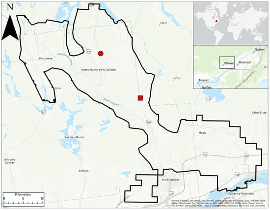
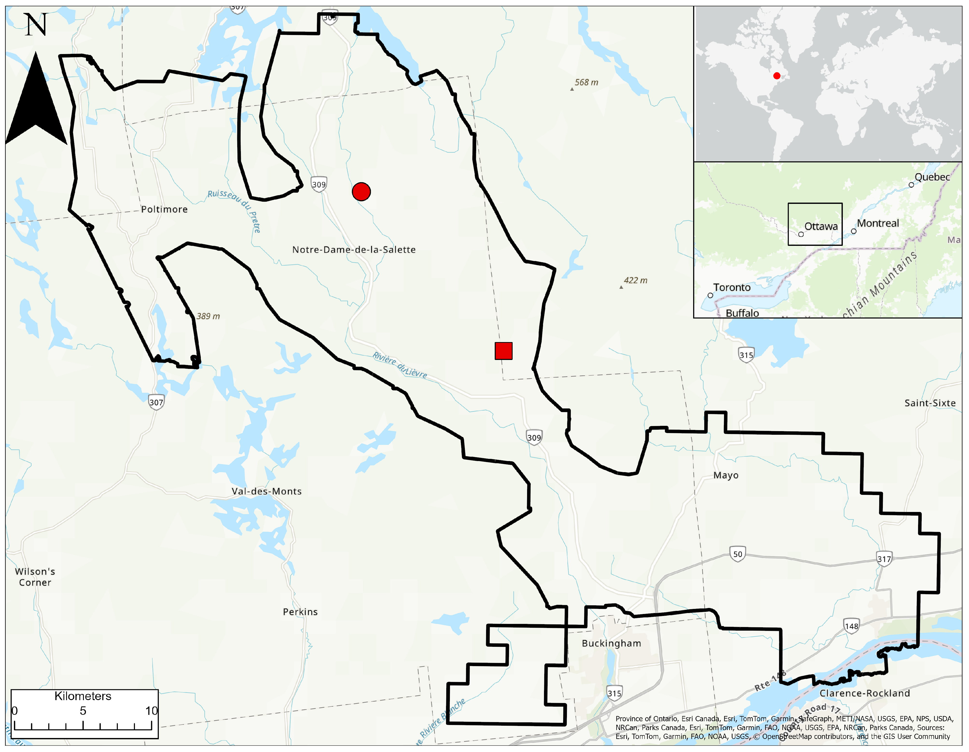
The study site is located approximately 30 km north of Ottawa in the WQSZ and is approximately 526 km2. Figure 1 below shows the extent of the study site alongside the Notre Dame de la Salette and Mulgrave and Derry landslides. The region is predominantly flat with only gently sloping terrain rarely exceeding 30 degrees, although short, steep slopes do exist near running water bodies. Geology is dominated by glacial sediments split between glacial tills and sensitive glaciomarine sediments (Leda clay).
Figure 1.
Study site located north of Ottawa city in the St. Lawrence lowlands showing the Notre Dame de la Salette landslide (red circle) and the Mulgrave and Derry landslide (red square).
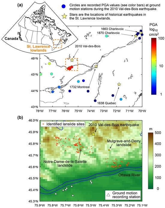
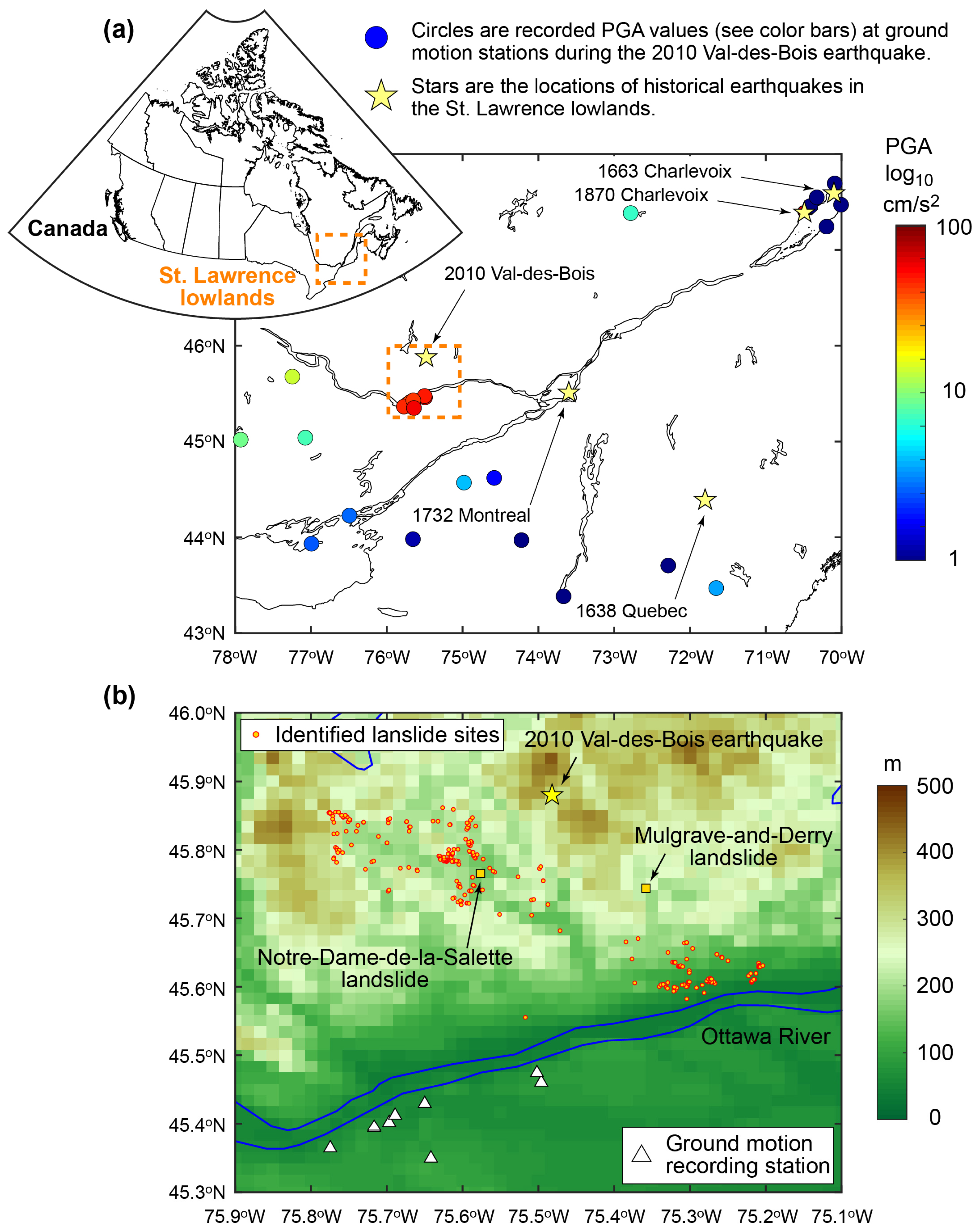
The 2010 Val-des-Bois earthquake occurred 50 km north of Ottawa in the WQSZ, but shaking was felt widely across the St. Lawrence lowlands with observable minor structural damage (e.g., chimney damage) in Ottawa [7]. The extent of shaking and landslide damage was limited because of the remote location in which the earthquake took place [8]. However, landslides in Leda clay were observed at Mulgrave-and-Derry (75.4874° W, 45.7202° N) and Notre-Dame-de-la-Salette (75.5807° W, 45.7931° N) areas (Figure 1 and Figure 2b) [9]. The aforementioned landslides are well-studied ETLs; however, no trigger-specific landslide inventories for the 2010 Val-des-Bois ETLs are available.
Figure 2.
(a) Regional map of the St. Lawrence lowlands and (b) local elevation map of the Western Québec Seismic Zone. In the regional map, the locations of the epicenter and ground motion recording stations are included. In the local map, the Mulgrave-and-Derry and Notre-Dame-de-la-Salette landslide sites, as well as the locations of the 263 identified landslides for the 2010 Val-des-Bois earthquake, are indicated on the map.
The closest ground motion recordings were made at seismographic stations in Ottawa, 45 to 50 km away from the epicenter, with a peak ground acceleration (PGA) less than 0.07 g [7] (Figure 2a below). It is hypothesized that many landslides were triggered in the near-fault region (epicentral distances of less than 25 km). Figure 2b shows seismic monitoring stations within the study site alongside potential ETLs in the context of the WQSZ elevation profile.
1.2. Background
Creating a landslide inventory, accompanied by relevant landslide parameters, such as slope angle and earthquake shaking characteristics, is important for evaluating trigger-specific landslide susceptibility and predicting the future occurrence of landslides in the region [3]. Traditionally, landslide inventories are created through literature review, field observations, aerial photography, and satellite imagery [10,11,12]. While helpful in demonstrating the extent of landslides in the region, landslide inventories such as these have difficulties in dating events and subsequently identifying the triggering mechanisms [13]. Incorporating triggering mechanisms into a landslide inventory, such as seismic loading, is useful when specifying the conditions that could initiate future landslides [14]. An investigation into the possible effects of ground motion on landslide initiation is presented to better understand the causes of these recorded landslides. To investigate a causal relationship between earthquake shaking and these near-fault landslides, it is necessary to estimate the level of ground shaking at the ETL locations. However, simple interpolation from observed ground motion is not appropriate because there are no seismic observations in the near-fault region [8]. Therefore, a ground motion model (GMM) consistent with the observed ground motions during the 2010 event can be adopted [8].
A potential use of a trigger-specific landslide inventory is to develop or calibrate a susceptibility model for regional landslide hazard assessments. [3] performed such an assessment for the St. Lawrence lowlands by using the Hazus method [15]. The Hazus method is a qualitative tool that evaluates landslide susceptibility based on relationships between slope angle, soil moisture content, and surficial geological material [15]. Adapted from works by [16,17,18], the Hazus method is traditionally focused on ground failures that are represented by a sliding rigid block. When applied to the St. Lawrence lowlands, the Hazus method results in a majority (58%) of the area being classified as “high” or “very high,” and the model shows limited predictive ability [3]. This means that for the region, the Hazus method is not necessarily a poor predictive model, but it is incapable of performing local predictions due to its reliance on a slope angle as a dominant predictor variable.
For instance, Refs. [1,19] conducted landslide susceptibility modeling using statistical regression and machine learning methods. The advantages of these methods are the incorporation of more landslide conditioning variables, such as geological shear strength, pore pressure, and wetness and the correlations between each variable and the occurrence of landslides, which allows for the addition of more distinguishing features between slopes. In such analyses, it is important to be aware of how many variables one includes to ensure the most accurate result is seen [19]. Ref. [20] applied random forest and artificial neural network techniques to their regression analyses and demonstrated significant improvements in landslide susceptibility analysis compared to conventional qualitative methods. Ref. [21] combined geographical information system (GIS)-based techniques and machine learning methods to identify landslide conditioning factors spatially. The use of conditioning factors included a maximum of fifteen factors, as well as a second analysis with seven factors to ensure accuracy [21].
1.3. Objectives
The current challenges for landslide susceptibility modeling in the St. Lawrence lowlands are the limited availability of a comprehensive database of ETLs (including local earthquake shaking intensities) and the lack of calibrated statistical and machine learning methods for the regional landslide data. This study makes several novel contributions to understanding ETLs in the WQSZ by achieving three objectives.
First, no earthquake-specific inventory exists for the WQSZ. We aim to develop the first trigger-specific, high-resolution (1 m) digital terrain model (HRDTM)-based landslide inventory for the 2010 Val-des-Bois earthquake. Second, we aim to capture both temporal changes (pre- vs. post-Val-des-Bois earthquake) and the detection of previously unmapped failures using difference-in-elevation HRDTMs, which is a novel approach for this region. Third, the incorporation of calibrated ground-motion estimates from GMMs to associate shaking intensity with each mapped landslide aims to add novel and rarely included seismic data to the landslide inventory.
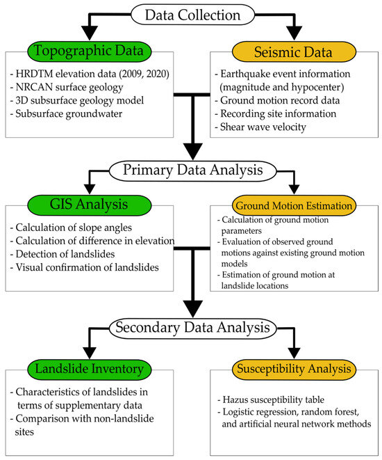
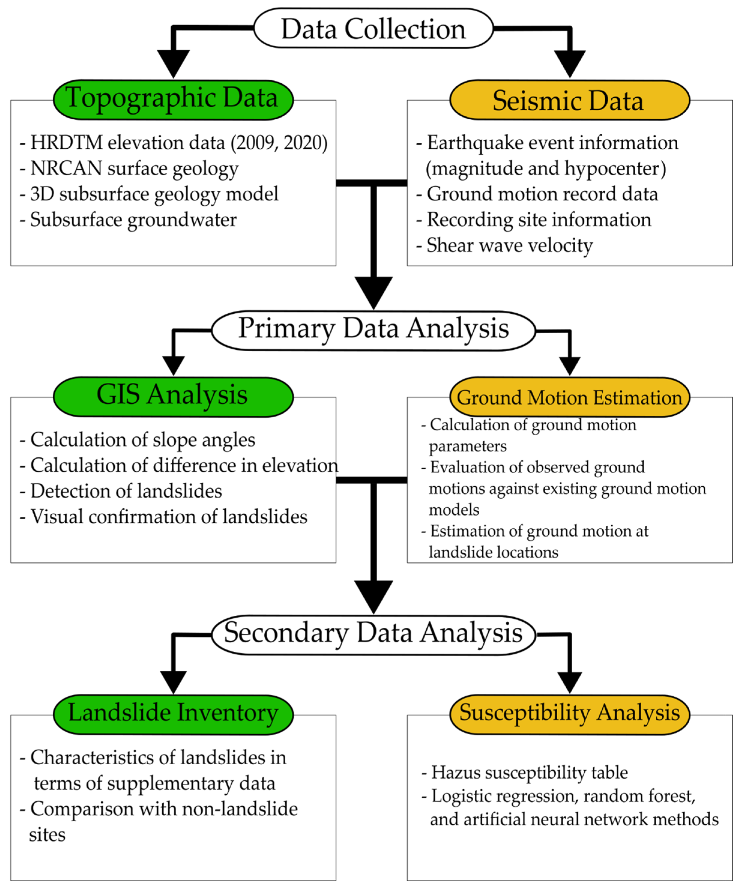
Based on the above objectives, the paper follows the flowchart in Figure 3. Section 2 introduces available data that are relevant for the study (e.g., topography, geological conditions, and seismic data) and develops a landslide database for the 2010 Val-des-Bois earthquake. Section 3 describes the methodologies used to achieve the three goals mentioned above. Namely, how the landslide inventory is created, how GMMs are selected, and how statistical and machine learning methods are applied to the inventory. Section 4 will cover the results of the susceptibility analysis. Finally, in Section 4 and Section 5, a discussion and conclusion surrounding the generation of an ETL inventory will be explored.
Figure 3.
Outline of the landslide inventory development and landslide susceptibility analysis for the 2010 Val-des-Bois earthquake.
This work presents the first HRDTM-derived, trigger-specific inventory for the 2010 Val-des-Bois earthquake, using pre- and post-event elevation differencing to identify and date landslides. The integration of calibrated ground-motion estimates with machine-learning susceptibility models represents a new methodology for the St. Lawrence lowlands, outperforming existing regional approaches such as Hazus. Finally, we demonstrate that integrating these datasets into machine learning models, namely logistic regression (LR), random forest (RF), and artificial neural network (ANN), can yield substantially more accurate susceptibility maps than Hazus for this region.
2. Materials and Methods
2.1. Data for Landslide Susceptibility Analysis
The data Sources for elevation, geological, soil characteristics, and water table are summarized in Table 1.
Table 1.
Sources for elevation, geological, soil characteristics, and water table data were used for developing a landslide inventory.
2.1.1. High-Resolution Digital Terrain Models
HRDTM data are provided through light detection and ranging (LiDAR) imaging data via the CanElevation Series [22]. For the WQSZ (Figure 2b), LiDAR images are grouped into 10 km by 10 km zones projected to the UTM NAD83 coordinate system and are presented at 1 m by 1 m resolution. HRDTM data for the study site are dated 2009 (pre-event) and 2020 (post-event). Both 2009 and 2020 HRDTM data are modified using the slope tool in ArcGIS Pro 3.30. Additionally, the elevations from 2009 and 2020 are subtracted from one another to create a difference-in-elevation raster at 1 m by 1 m resolution, which enables visual identification of potential landslides by showing areas of erosion and deposition. This difference-in-elevation raster represents topography before and after the 2010 Val-des-Bois earthquake and confines topographical changes to an approximate date of initiation, which can be hypothesized to have occurred during the Val-des-Bois earthquake.
2.1.2. Surface Geology
Geological data are obtained from the Geological Society of Canada (GSC) [23,24] and serve for different purposes in the analysis of landslide identification. Ref. [23] is used for classifying the surficial geological layer within the study site, but it does not provide information regarding the depth or thickness of geological materials. The surficial geological data used in this paper are available from the GSC Surficial Geology map [23]. The primary use of geological models is to identify prominent Leda clay deposits, as they are the assumed sliding layers due to their high sensitivities [27].
There are five classes of geology being considered. Offshore and littoral glaciomarine sediments, which are characterized by their abundance of Leda clay. Alluvial and glaciofluvial sediments, which may contain traces of Leda clay, and glacial sediments represent a veneer layer [23]. The second geological database, used for the purposes of shear wave velocity assignment, was a subsurface, 3D geological model [24,27]. The following explains the shear wave velocity (Vs, in m/s) equations and values used, where z refers to the depth of the geological layer in meters. Readers are referred to [25] for explanations on how these equations and values were developed.
- Surface sand (Vs = 119 + 8.1 × z0.5)
- Clay (Vs = 119 + 8.1 × z0.5)
- Basal till (Vs = 1500)
- Bedrock (Vs = 2500)
2.1.3. Shear Wave Velocity Profile
Average shear wave velocity in the upper 30 m (Vs30) is used to aid in the understanding of local site conditions relative to shaking intensity. Softer soils, such as Leda clay, typically experience higher intensity shaking than harder soils, such as gravel, since their Vs30 is lower [28]. The Vs30 model used in this study is adopted from [25] and is based on the 3D geological model created by an earlier version of [24]. Representative values of shear wave velocity for surficial sand, clay, basal till, and bedrock layers are assigned to calculate the Vs30 values for individual sites. When comparing Vs30 to the surficial geological classifications of [23], it is expected that Vs30 is consistent with the landslide susceptibility ranking of geologies, such that a higher Vs30 corresponds to a harder geology or shallow surficial soil layers.
2.1.4. Well Data
Water table data are interpreted from borehole data from the hydrogeological information system (HIS), maintained by the Government of Québec [26]. Interpretation is derived from taking the depth to water measurement at each borehole and applying the natural neighbor function in ArcGIS to it. This creates a 2-dimensional plane across the study site with cells at a resolution of 1 m by 1 m, with each cell representing the depth to the water table. This value can be used as a proxy for soil wetness by classifying water table depths greater than 10 m as dry and shallower tables as wet [15].
2.2. Development of the Landslide Inventory with Pre- and Post-Event HRDTM Imagery
Ground failures potentially caused by the 2010 Val-des-Bois earthquake that occurred in the WQSZ are identified by examining the difference in elevation map based on the 2009 and 2020 HRDTMs and by inspecting Google Earth images at different times (before and after the earthquake) to confirm that the identified landslides can be associated with the 2010 earthquake with confidence. The following sections describe this process using various examples, such as the Notre-Dame-de-la-Salette landslide (Figure 4).
Figure 4.
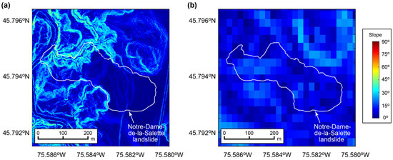
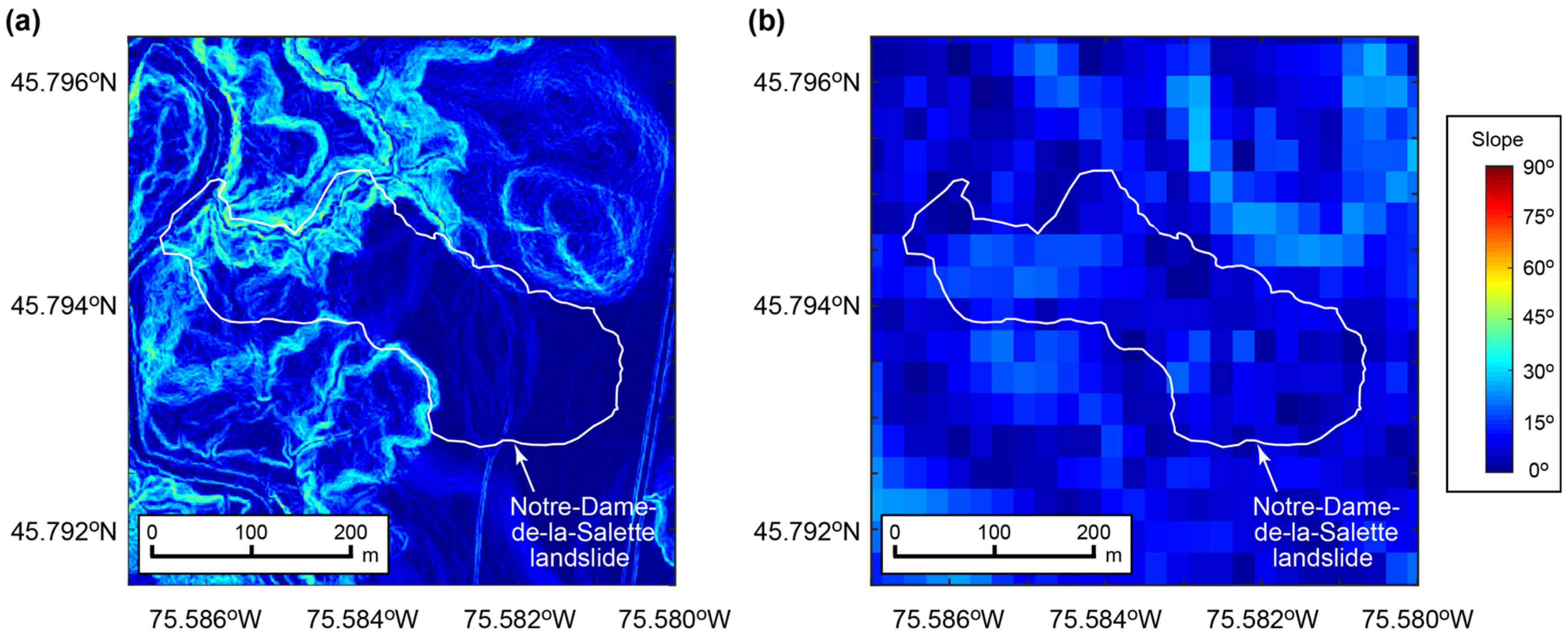
Slope angles at the Notre-Dame-de-la-Salette landslide location in: (a) 1 m resolution HRDTM and (b) 20 m resolution.
2.2.1. Notre-Dame-de-la-Salette Landslide
Figure 4a,b show slope angle maps based on the 1 m and 20 m DTM datasets for the location of the Notre-Dame-de-la-Salette landslide. Using high-resolution topographical data is important in aiding the identification of potential landslide triggers and features previously invisible at lower resolutions (e.g., rivers). In the 20 m resolution imagery, slopes between 40 and 50 degrees are not clearly visible or defined. This becomes important for landslide analysis as riverine features are known landslide initiation locations due to erosion and steep embankments [29]. Moreover, due to the unique retrogressive behavior of Leda clay landslides, where short, steep slopes can trigger a failure that moves into more stable terrain, being able to visualize these slopes and the surrounding terrain is important for landslide hazard analysis [29,30]. For the Notre-Dame-de-la-Salette landslide, the maximum difference in elevation (from 2009 to 2020) is 14.4 m. The positive elevation differences (i.e., erosion) appear in the crown part of the landslide, while negative differences (i.e., deposition) are mainly located at the foot part of the landslide.
2.2.2. Development of the Entire Landslide Inventory
Key identifiers of landslides from the HRDTM perspective are sections of reduced (erosion) and increased (deposition) elevation, as demonstrated for the Notre-Dame-de-la-Salette landslide in Figure 4. Therefore, the first step is to detect the landslide features using the difference-in-elevation data based on the 2009 and 2020 HRDTM raster maps. Potential landslides are identified visually across the study site, and their footprint boundaries are digitized individually in ArcGIS. The difference in elevation data serves as novel pre- and post-event imagery, as the hypothesized trigger for landslides in the study site is the 2010 Val-des-Bois earthquake.
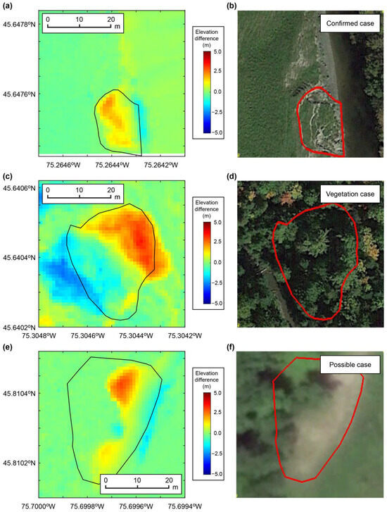
Once a preliminary landslide inventory is generated by identifying locations of notable erosion and deposition, each potential landslide is verified with Google Earth imagery. Through the verification process, each landslide site is carefully examined and is classified into three categories. Figure 5 shows examples of the three categories. First is whether the landslide appears at the earliest available image following 2010. A landslide visible in the 2012 imagery but not visible in the 2009 imagery is considered to have been caused by the 2010 Val-des-Bois earthquake and is labeled as a “confirmed case” in Figure 5a,b. On the other hand, a landslide absent in the 2009 and the 2012 Google Earth images (note: in most cases, 2012 is the earliest available imagery), but visible in the 2015 imagery, is considered not to have occurred as a direct result of the 2010 Val-des-Bois earthquake. These events are then discarded.
Figure 5.
Elevation difference color maps (a,c,e) and Google Earth images (b,d,f) of three landslide categories. (a,b) confirmed case, (c,d) vegetation case, and (e,f) possible case.
Second is how visible the landslides are. In many cases, vegetation obstructs the bare earth, and landslides are not clearly visible. In these cases, the landslides are kept as potential events and are labeled as a “vegetation case” due to the HRDTM difference in elevation data showing a change in elevation that could represent a landslide, but visual confirmation was not possible. This highlights the usefulness of a high-resolution bare-earth topographical dataset for landslide identification. These potential landslides are currently being tentatively kept. The third case corresponds to situations where other obstructions or topographical features make landslides difficult to identify. These are also kept but labeled as “possible cases” in Figure 5e,f. Additionally, the landslide shape is analyzed. In some cases, large changes in elevation are caused by excavation or other anthropogenic sources. These events are discarded.
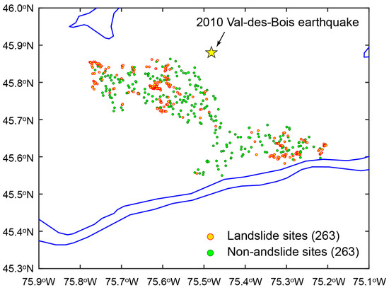
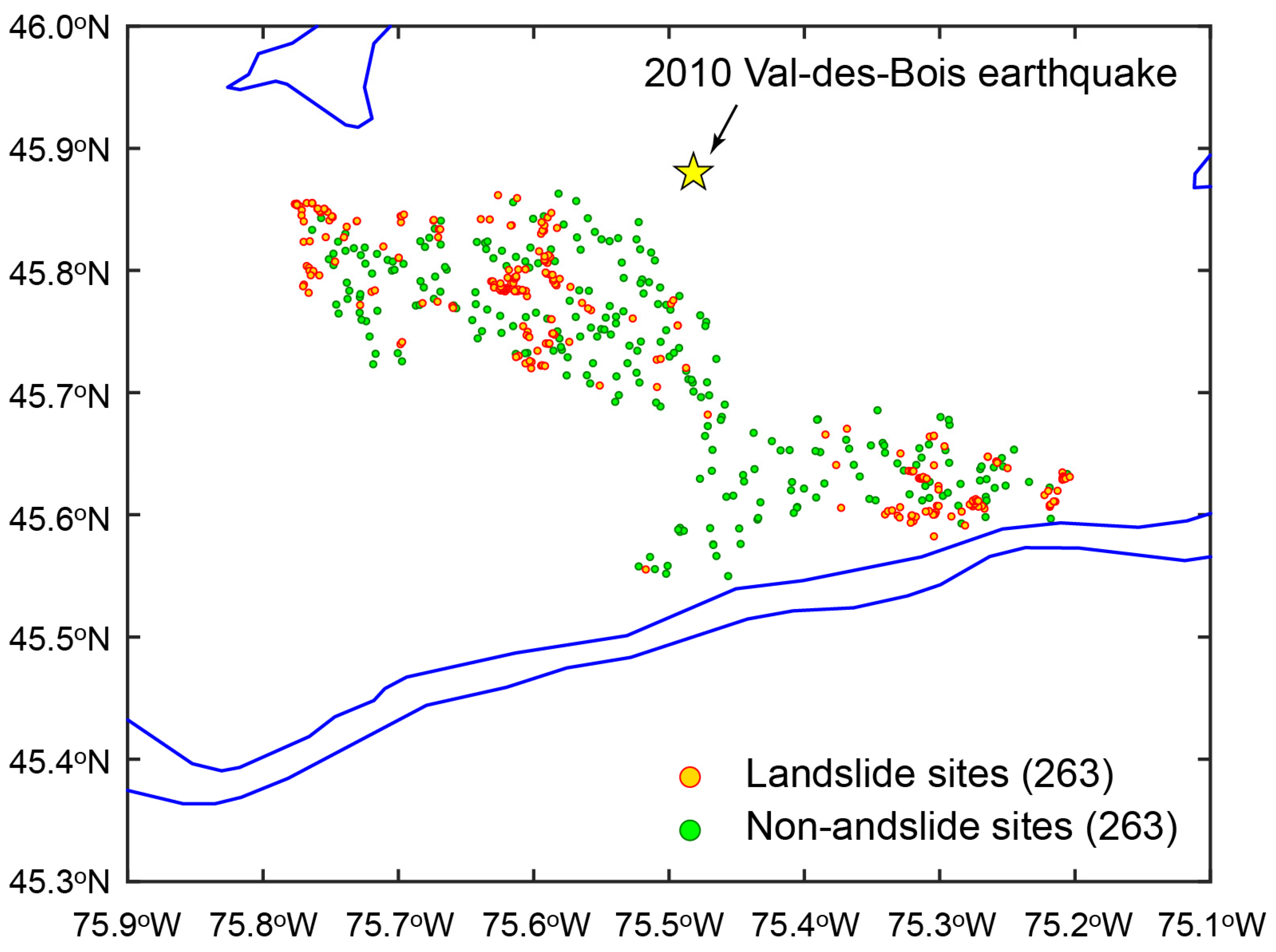
For landslide susceptibility methods, similar data for non-landslide locations are necessary. 263 non-landslide sites were randomly selected within the study site and were visually inspected to ensure they did not intersect with the landslide sites nor were within waterbodies. These are combined with the previously identified 263 landslides in the WQSZ to create the final landslide inventory and can be seen in Figure 6.
Figure 6.
Map of the landslides and non-landslide locations.
2.3. Estimation of Ground Shaking at Landslide Sites and Ground Motion Model Selection for the 2010 Val-des-Bois Earthquake
This section presents a method to estimate ground shaking experienced at the identified landslide sites. Although ground motions were recorded during the 2010 Val-des-Bois earthquake (see colored circles in Figure 2a), there were no direct ground motion measurements in the near-source region where most of the landslides were triggered. For this purpose, available ground motion records were processed and compared with ground motion models that are applicable to Eastern Canada [31,32]. As a ground motion parameter, PGA is considered because it is often adopted for the sliding rigid block analysis by [16]. Through such comparisons, the best-fitting ground motion model can be identified and used for estimating PGA values for the landslide inventory. The information on landslide triggering factors can be useful for evaluating the minimum seismic loading to trigger landslides in the St. Lawrence lowlands and for investigating a relationship between the landslide occurrence and earthquake shaking level as part of landslide susceptibility analysis [14].
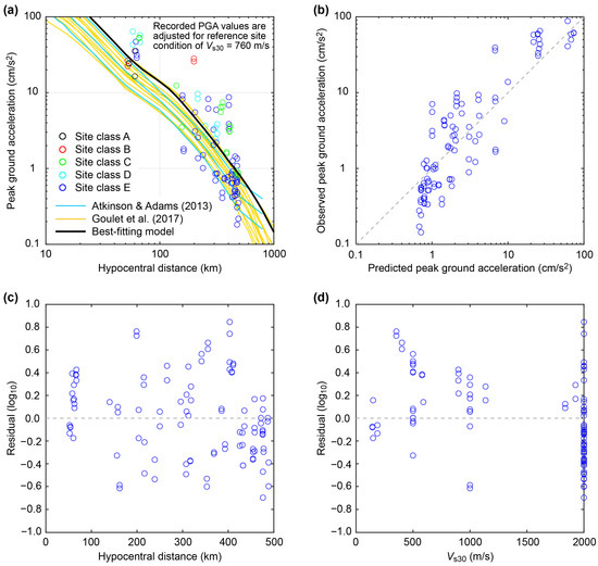
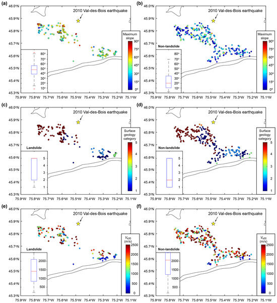
Ref. [8] compiled accelerograms that were recorded at seismographic stations in Eastern North America during the 2010 Val-des-Bois earthquake. By analyzing these available ground motion data, the observed PGA values are plotted against hypocentral distance in Figure 7a. Since the moment magnitude of the 2010 Val-des-Bois earthquake is estimated as Mw 5.0 [7], the point source approximation of the rupture is suitable (i.e., the source-to-site distance can be well represented by the hypocentral distance instead of the rupture distance). PGA data are distinguished based on-site classes A to E as specified by the National Building Code of Canada [33].
Figure 7.
(a) Comparison of the observed PGA values with ground motion models of [31,32]. The observed PGA values are adjusted for the reference site condition of Vs30 = 760 (m/s), while the ground motion models are set for the same Vs30 value. (b) Comparison of the observed and predicted PGA values. (c) Ground motion residuals with respect to hypocentral distance. (d) Ground motion residuals with respect to Vs30.
In Eastern Canada, the most recent seismic hazard assessment [34] adopts two sets of ground motion models that are applicable to the WQSZ. The ground motion model by [31] specifies three median models to capture epistemic uncertainty, while the ground motion model by [32] comprises thirteen median models. Figure 7a includes, in total, sixteen median PGA prediction equations by considering the reference site condition of Vs30 = 760 m/s. After adjusting the site conditions of the recording stations for hypocentral distances of less than 500 km (in total, 100 recordings were adopted), PGA observations are corrected and then compared with predicted PGA values based on the sixteen ground motion models. The root mean square errors in logarithmic space are evaluated for all sixteen ground motion models to identify the best-fitting prediction equation.
The identified best-fitting ground motion model is shown with the thick solid curve in Figure 7a. This model fits well with the observed ground motion data in Ottawa (which are shown at hypocentral distances between 50 km and 70 km). To demonstrate the goodness of the fit of the identified ground motion model, Figure 7b shows a scatter plot of the observed and predicted PGA values. The agreement between the observations and predictions is judged to be satisfactory, especially for larger PGA values. In addition, to show the unbiased trends of the best-fitted ground motion model against hypocentral distance and Vs30, residual plots for these two explanatory variables are shown in Figure 7c,d. No obvious trends are detected in these residual plots. Overall, it is concluded that the identified ground motion model can be used to extrapolate ground motion for the near range, which is applicable to the landslide sites.
2.4. Landslide Susceptibility Modeling Methods
A landslide susceptibility analysis evaluates the relative landslide occurrence likelihood in terms of environmental variables [1,3,20]. In developing such relationships between landslide occurrence and explanatory variables, different forms of mathematical functions can be adopted (i.e., logistic regression). For instance, Hazus [22], which is one of the widely accepted approaches to susceptibility for ETLs, employs a table format to categorize potential landslide cases into indices. With larger sets of explanatory variables, more complex functional forms can be considered [19,20]. Three machine learning algorithms, namely, logistic regression, random forest, and artificial neural network, are implemented to evaluate landslide susceptibility of the developed inventory for the 2010 Val-des-Bois earthquake. All three methods are implemented using MATLAB R2023a. Additionally, all models, including Hazus, are tested on the same data sets with the same resolutions for consistency purposes.
In evaluating the performance (goodness of fit) of a model, the root mean squared error is computed by considering five-fold cross-validation (i.e., the dataset is divided into 80% training data and 20% testing data, and this training-testing process is repeated five times by considering different non-overlapping testing data). Five-fold validation was selected to ensure all parts of the data at some point are used to both train and test the model. Landslides in the inventory are categorized as 1 (landslide) or 0 (non-landslide), and analysis is done where all potential landslide cases (i.e., confirmed, vegetation obscured, and possible) are classified as landslides, as well as the various permutations possible from that set. This checks the quality of our inventory for susceptibility modeling and prediction.
2.4.1. Hazus Method
The Hazus landslide susceptibility method produces discrete landslide indices (I to X or None) based on three conditioning factors, i.e., geological type, soil wetness, and slope angle (Table 2). The influences of the geological type (A, B, and C) and the slope angle are significant on the final landslide index, noting that Leda clays are classified into Group C (i.e., high susceptibility). A limitation of the Hazus method for Leda clay sediments in the St. Lawrence lowlands is that a high index value of VII is assigned to flat areas (slope angles less than 10 degrees), while when slopes are steeper than 10 degrees, the index values of IX and X are given. Consequently, the Hazus method will serve as a conservative approach, generating many false positives. On the other hand, it does not have the ability to distinguish the relative landslide potentials within the same category. From regional landslide assessment perspectives, despite the limitations, the Hazus method serves as a benchmark, as this method has been adopted by [3] for the St. Lawrence lowlands.
Table 2.
Landslide susceptibility classification based on slope angle, geological group, and soil moisture content [15].
2.4.2. Logistic Regression
A binomial logistic regression [35] is carried out to characterize the landslide occurrence Y (1: landslide occurrence and 0: no landslide) by considering explanatory variables X, consisting of slope angle, surface geology, groundwater depth, Vs30, sediment layer thicknesses, and PGA. The relationship between Y and X is expressed as:
where p(Y) is the probability of one category (e.g., landslide occurrence). The parameter estimation is performed by maximizing the loglikelihood function. Logistic regression is particularly useful for three aspects in interpreting the model fitting results. First, model coefficients can be estimated with their confidence intervals, thereby, the statistical significance for each explanatory variable can be assessed. Second, the sign of the regression coefficient gives a sense of dependence. Third, the model performance metric, such as root mean squared error, can be used and compared with results from other fitting methods.
2.4.3. Random Forest Method
Random forest utilizes decision trees to make predictions and is applicable to addressing both regression and classification problems [36]. Its primary advantage is that it does not make assumptions about the distribution of the data and can capture complex patterns in the data based on an ensemble of decision trees [19]. A random forest model constructs multiple decision trees during training using a bootstrap sample drawn from the dataset, and outputs the mean predicted value of individual trees (i.e., bagging). Bagging reduces overfitting and improves the accuracy and stability of the model. When creating a decision tree, the algorithm calculates the root mean squared error of each possible split for each feature. Then, the algorithm searches for a feature that best splits the data by achieving the lowest root mean squared error. The splitting process of the decision tree stops when the root mean squared error cannot be improved, or the split times reach the maximum number. In this study, the quantity of decision trees is set to 500 (note: a sensitivity test regarding the tree size is carried out and the results do not depend on this setup). The final landslide prediction of the trained random forest model is acquired by taking the mean of predictions made by all decision trees within the forest.
2.4.4. Artificial Neural Network
An artificial neural network has a layered structure consisting of interconnected nodes (i.e., neurons) and can be trained based on suitable training algorithms by adjusting the weights of the interconnected nodes adaptably [19]. A well-calibrated neural network model can recognize patterns, classify data, and forecast future events. To avoid overfitting, the performance of the trained neural network is evaluated by using testing data. By adopting the cross-validation scheme for the root mean squared error evaluation, the training-testing process is repeated five times in this study. A so-called feedforward neural network, consisting of an input layer, 10 hidden layers with 30 nodes, and an output layer, is employed. Preliminary sensitivity tests indicate that the results do not change significantly by considering different configurations of neural network (varied in the range of 5 to 30 layers and 10 to 50 nodes). Within the MATLAB R2023a computing environment, several training algorithms are available. Among those tested, the Levenberg–Marquardt algorithm (damped least squares) is used in this study, which results in stable performances.
3. Results
3.1. Characteristics of the Landslide Inventory
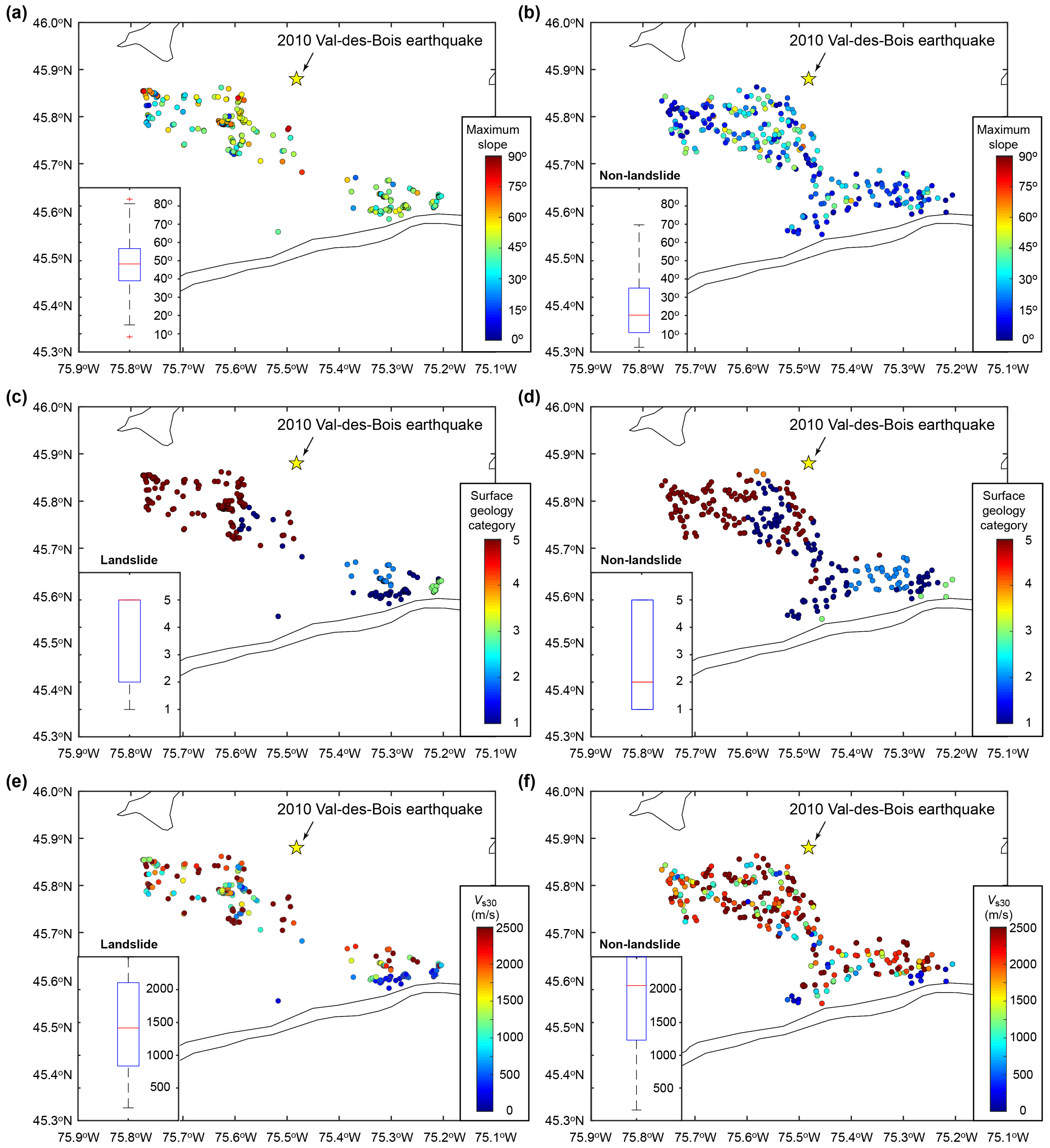
Traditional characteristics of landslide and non-landslide sites are investigated. Figure 8 shows maps of the maximum slope, surface geology, and Vs30, accompanied by the corresponding box plots of the data in the subpanels. The landslide and non-landslide data are visualized separately. Of the selected variables, the maximum slope is the strongest predictor for landslides in the WQSZ. Landslide sites are associated with steeper slopes than non-landslide sites based on the comparison of Figure 8a,b. The influence of surface geology is more complex, as demonstrated in Figure 8c,d. In the northwestern part of the WQSZ, there are areas with glacial sediments (surface geology class 5), where many landslides occurred.
Figure 8.
Data characteristics of the landslide (a,c,e) and non-landslide (b,d,f) sites. (a,b) Maximum slope, (c,d) surface geology, and (e,f) average shear-wave velocity in the top 30 m.
In these areas, typically thin layers of till were mobilized, while in the southeastern part of the WQSZ, more areas had mobilized Leda clay (surface geology classes 1 to 4). When the sites contain steep slopes (i.e., Figure 8a vs. Figure 8b), landslides tend to be triggered. Note that even when Leda clay sediments are present in shallow slopes (less than 30 degrees), slopes may not fail despite the high sensitivity of the geology (see area between 75.5° W and 75.6° W and between 45.7° N and 45.8° N). Therefore, the presence of Leda clay alone may not be the primary predictor for landslide triggering. Finally, the comparison of Figure 8e,f indicates that Vs30, which represents the stiffness of near-surface soil, affects the landslide occurrence. The landslide sites are associated with lower Vs30 values than the non-landslide sites. These differences may reflect various features of near-surface soil deposits (e.g., thickness of sedimentary layers and presence of Leda clays).
The creation of the trigger-specific landslide inventory demonstrates how HRDTM data can be used effectively in identifying potential mass movement events. Specifically, the use of the difference in elevation data in adding temporal detail to landslide inventories. Since a difference in elevation requires pre- and post-event data, any potential landslides must have occurred between the dates when the HRDTM was created. This allows inventories created through this method to estimate the age of the landslides as well as identify potential triggering events, such as the 2010 Val-des-Bois earthquake in our case. Additionally, the use of HRDTM gives high-quality results about topography from a remote sensing perspective, such as identifying slope conditions near riverine features where short and steep slopes are present; something not possible at lower resolutions. The landslide inventory is also large, with 263 probable cases ranging in size from a few meters in diameter to upwards of 200 m, showing the ability of the HRDTM to aid in identifying difficult-to-spot landslides, which may be too small to identify using traditional methods.
3.2. Estimation of PGA at the Landslide Sites and Ground Motion Model Selection for the 2010 Val-des-Bois Earthquake
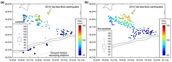
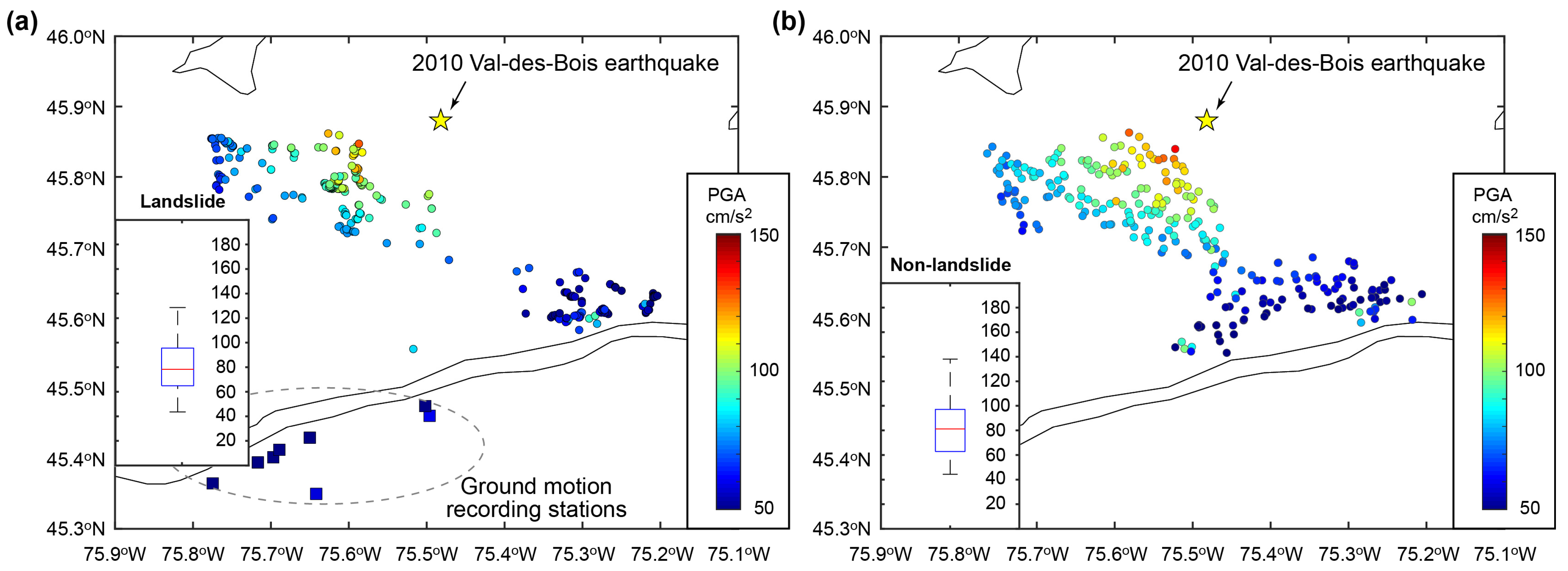
The estimation of the PGA values at the landslide sites for the 2010 earthquake is carried out by using the best-fitting ground motion model. The predicted PGAs for the landslide sites can be evaluated by adopting the median PGA model and by adjusting for local site conditions based on Vs30 [8]. As such, median PGA shake maps at landslide and non-landslide sites are shown in Figure 9, accompanied by box plots of the PGA data. The results show that in the near-source region, PGA values at the sites in the landslide inventory reach 0.15 g, which decreases to 0.05 g farther away from the epicenter. Because the landslide and non-landslide sites are distributed within the same region, PGA values of these two groups overlap. It is noteworthy that the PGA values shown in Figure 9 are the deterministic predictions. Since variability associated with the prediction models is generally large (see Figure 7a,b), probabilistic estimates of the PGA values at the landslide and non-landslide sites can also be produced [37]. When such variability is considered, PGA values at the landslide locations could reach 0.25 g. In interpreting the estimated (median) PGA values for the 2010 earthquake, such variability should be considered. Another important observation from Figure 8 is that some of the Leda clay slopes could fail with low PGA disturbances of less than 0.1 g (when other conditioning factors, such as steep slopes, are present).
Figure 9.
Predicted PGA values of the (a) landslide and (b) non-landslide locations.
3.3. Results Based on the Benchmark Hazus Method
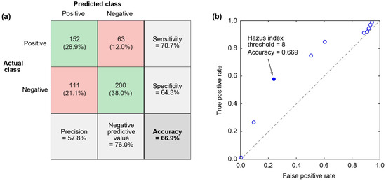
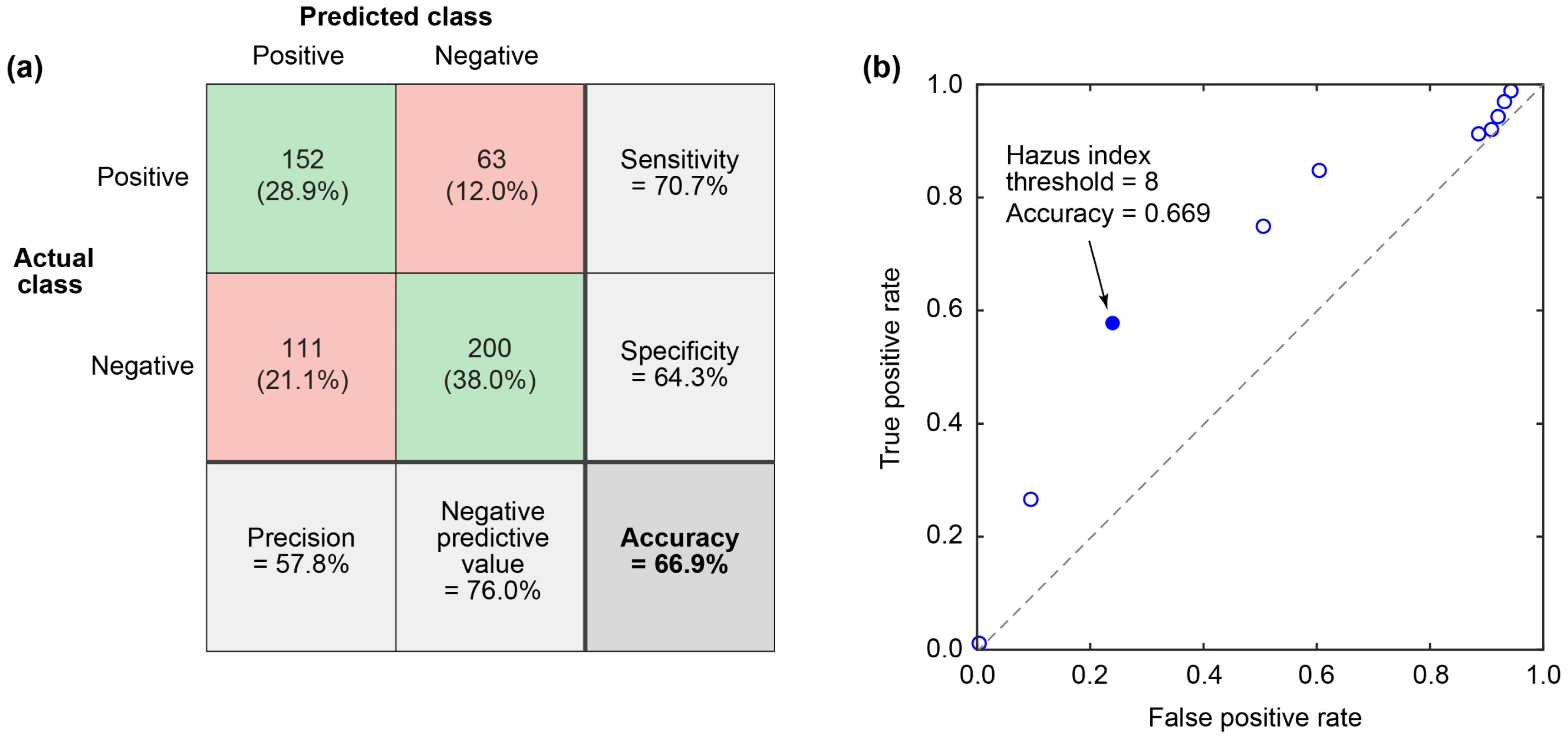
The landslide susceptibility analysis is first conducted using the Hazus method. The outputs from the Hazus method are expressed in terms of landslide susceptibility indicators I to X [15]. To convert these to binary outcomes, a threshold to predict the occurrence or non-occurrence of a landslide is varied from I to X and then for each threshold value, a confusion table is generated. An illustration of a confusion table is shown in Figure 10a, which is developed for a threshold of XIII. From a confusion table, several performance metrics can be calculated, including accuracy, sensitivity, and precision [37]. Moreover, when true positive rates and false positive rates from individual confusion tables with different threshold values are plotted, a receiver operating characteristic (ROC) curve can be obtained, as shown in Figure 10b. The area under the ROC curve (AUC) can be adopted to quantify the overall performance of the method [38]. For the Hazus method together with the developed landslide inventory, the optimal threshold is found to be VIII with an accuracy of 66.9%, indicating that the Hazus method is most accurate when calculated sensitivities are within the threshold range of VIII–X. This accuracy is considered a benchmark in evaluating the relative performance of the machine learning-based landslide susceptibility analysis results. It is important to note that the accuracy of the Hazus method varies depending on the threshold of susceptibility used. In other words, the Hazus method drops in accuracy to approximately 50% (i.e., chance) when it considers landslides of susceptibilities across all possible discrete susceptibilities from None to X.
Figure 10.
(a) Confusion matrix and (b) receiver operating characteristic plot for the Hazus method.
3.4. Logistic Regression Results
The logistic regression method offers a clear interpretation of the landslide susceptibility analysis. For this reason, results from logistic regression are discussed first. Table 3 summarizes the logistic regression analysis results (i.e., coefficients, standard errors, and p-values) with and without PGA as an explanatory variable. Inspecting the results without PGA indicates that the coefficients for surface geology, maximum slope angle, and Vs30 are statistically significant and have direct and inverse relationships, respectively. The positive trend of landslide susceptibility with respect to surface geology type reflects the frequent occurrence of shallow landslides in till deposits, whereas its positive trend with respect to maximum slope angle is consistent with the physical situation [3]. On the other hand, the negative trend of landslide susceptibility with respect to increasing Vs30 is plausible as the presence of hard rock closer to the ground surface would reduce the chance of landslide occurrence [28]. The other two variables, i.e., depth to water table and sediment thickness, are not significant factors in the models developed herein. Note that when Vs30 is removed from the predictor variables, sediment thickness shows statistical significance. A high negative correlation between sediment thickness and Vs30, as seen in Figure 11, can explain this outcome, as seismic waves generally travel more slowly through thicker and softer material.
Table 3.
Logistic regression model coefficients.
Figure 11.
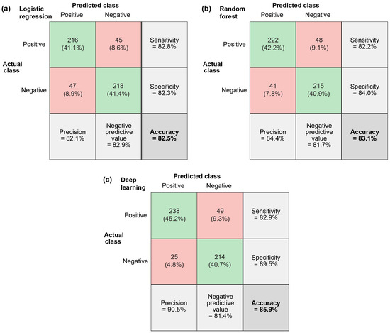
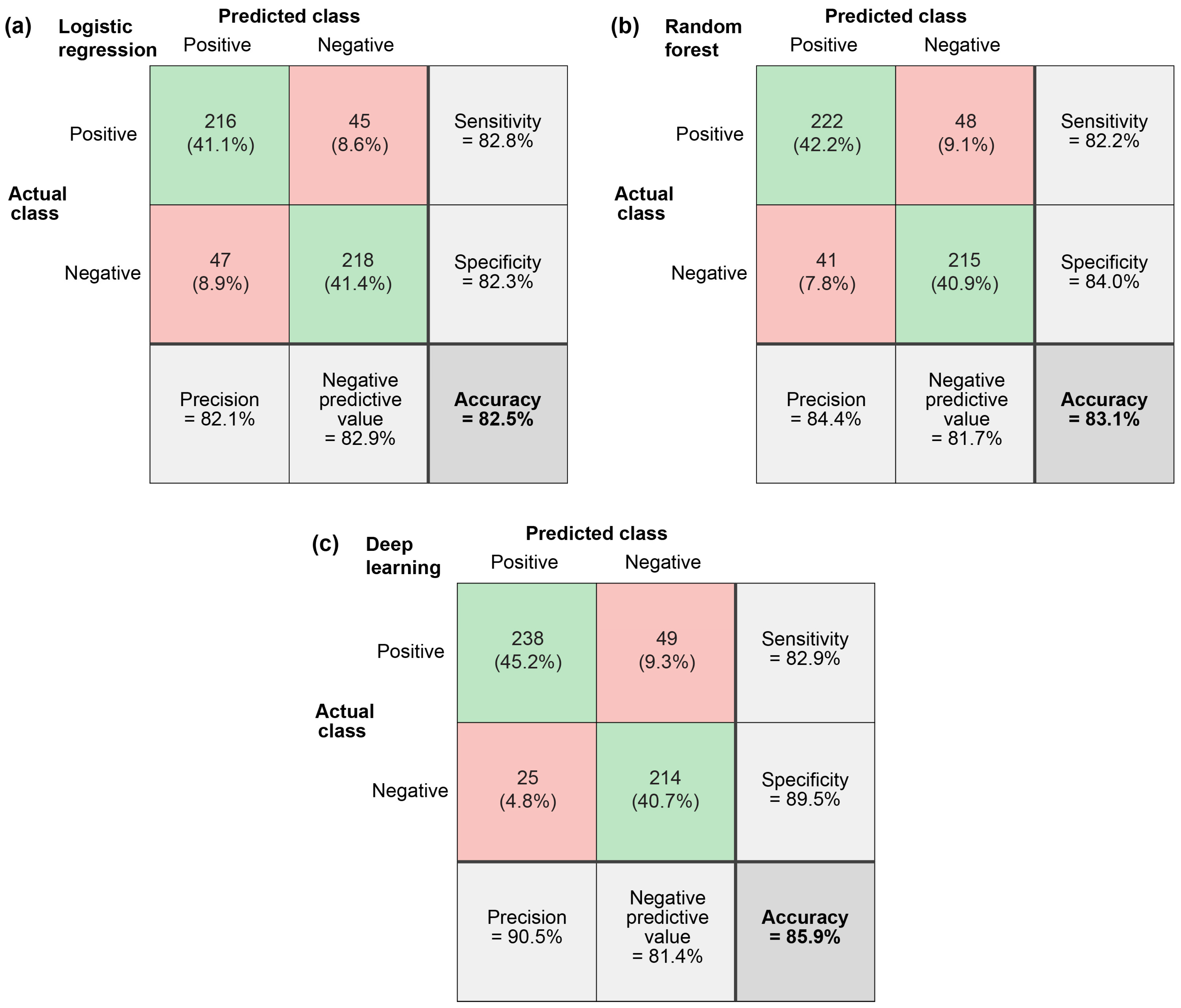
Confusion matrix results of landslide susceptibility models based on: (a) logistic regression, (b) random forest, and (c) artificial neural network.
Next, logistic regression analysis is conducted, and PGA is added as a predictor variable in Table 3. The results of the variables related to the sliding slopes are largely unchanged in terms of significance and sign of the estimated coefficients. The coefficient for PGA is statistically significant but with a negative sign. This contradictory result seems to be caused by two conditions. One is that median PGA values of the landslide and non-landslide sites overlap, causing a discrepancy as to their effect on the predictions, as can be seen in the maps of landslide locations and the respective predicted PGA values (Figure 8). Note also that actual PGA values experienced at these sites may be different from the median PGA values. The second condition can be attributed to the occurrence of shallow landslides of till sediment in the northwestern part of the study site, where PGA values become inherently small but sufficient (along with steep slopes) to trigger landslides. While some explanations could be offered for the landslide susceptibility model, including PGA, the results are still counterintuitive. Although the depth to the water table and sediment thickness do not show significant regression coefficients, these two variables are retained for random forest and neural network methods because they can predict landslide occurrence by capturing complex patterns and nonlinear effects. It should be emphasized, however, that when logistic regression models are used for prediction purposes, the depth to the water table and sediment thickness variables should be removed from the analysis.
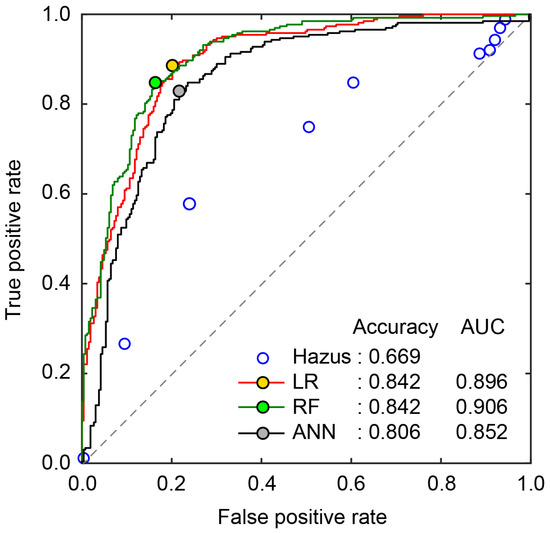
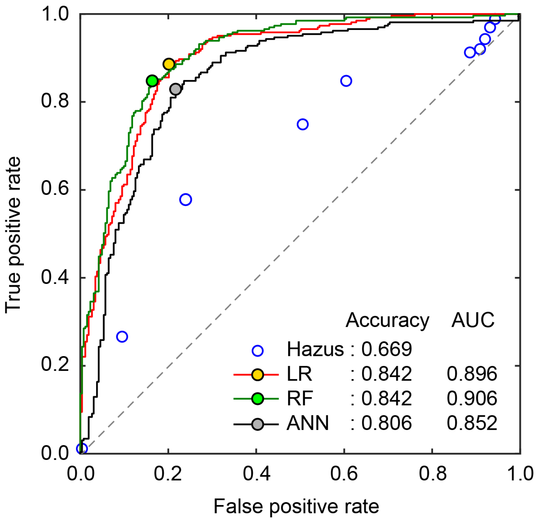
The performance of the logistic regression model is evaluated using the confusion matrix in Figure 11a and the ROC curve in Figure 12, noting that PGA is not included in the conditioning variables. Since landslide occurrence is a binary value (i.e., 0 for non-landslide and 1 for a landslide), the statistical models use simple rounding with a threshold of 0.5 to ensure outputs are either 0 or 1. The accuracy of the logistic regression is 82.5%, as shown in Figure 11a. When the threshold is adjusted to achieve the highest accuracy, the accuracy value reaches to 82.5% with AUC = 0.896. Note that the logistic regression model outperforms the Hazus method significantly, as the ROC curve is closer to the top-left corner (i.e., prediction capability of 100%).
Figure 12.
Comparison of receiver operating characteristic plots for the Hazus, logistic regression (LR), random forest (RF), and artificial neural network (ANN) methods.
It is also useful to report the accuracy and AUC values for cases where different conditioning variables are included in the model. Table 4 lists the accuracy and AUC values for two additional cases. The first case includes PGA as a conditioning variable, while the second case adopts the average slope angle, rather than the maximum. The latter case is more useful in situations where high-resolution data are not available for calculating slope angles, resulting in more gentle values of slope angles similar to what is expected with lower resolution topographical data. The inclusion of PGA leads to slightly improved values of accuracy and AUC values, which may be questionable given that landslide locations are not uniform throughout the study site. This can cause PGA to be skewed towards the lower end of PGA values because there is a clustering of landslide locations further away from the epicenter than the more uniform (randomly generated) non-landslide locations. Using the average slope angles to characterize the pre-failure condition of the slopes results in lower accuracy and AUC values compared to when the maximum slope angles are used.
Table 4.
Summary of the performance metrics for different landslide susceptibility modeling cases.
3.5. Random Forest Results
The same set of landslide susceptibility analyses was conducted using the random forest method. The results are shown in Figure 11 and Figure 12, and Table 4. The overall results of the random forest method are similar to those of the logistic regression method, but with slightly higher accuracy and AUC values. However, these differences are relatively small, and therefore, the logistic regression and random forest methods are equally capable of predicting the landslide occurrence using the selected predictor variables. One interesting feature is seen by inspecting the results shown in Table 4. The inclusion of PGA does not result in increased accuracy, unlike the logistic regression method, potentially indicating that the negative relationship between landslide susceptibility and PGA, seen for logistic regression, is not robust. The consideration of the average slope angle results in smaller accuracy and AUC values compared to when the maximum slope angle is used. However, the decrement of these performance metrics is smaller than that of the logistic regression.
3.6. Artificial Neural Network Results
The set of landslide susceptibility analyses that were previously discussed is repeated using the artificial neural network method, and the results are shown in Figure 11 and Figure 12 and Table 4. It is observed that the predictive performance of the ANN model is lower than that of the logistic regression and random forest methods, but still significantly higher than the Hazus method.
4. Discussion
4.1. Machine Learning vs. Hazus Susceptibility Model
Machine learning techniques were performed and compared to the Hazus method for accuracy using (1) only the Hazus variables of slope, geology, and moisture content, (2) all tested variables (see Supplementary Materials), and (3) only seismic variables. It was determined that Hazus is the least accurate method and that it typically underperforms the machine learning methods by 15 to 30%, depending on the threshold used. This metric comes from overall accuracy assessment, as well as being supported by the AUC values described in Table 4 and Figure 12.
It is possible that slope angle, while important, may not be sufficient as a sole predictor in landslide susceptibility analysis specifically for Leda clay due to the high sensitivity. Instead, the interactions between multiple conditioning factors may be better at predicting susceptibility. For future susceptibility analysis, identifying ways to incorporate the retrogressive nature of Leda clay slopes, where nearby stable terrain can become mobilized, could be useful in better identifying potential landslide risk. However, the methods proposed in this study show the applicability of a remote sensing-based approach for landslide susceptibility analysis in the St. Lawrence lowlands.
4.2. Incorporation of Landslide Conditioning Variables into Prediction Models
Despite improvements in predictive ability, machine learning techniques in this study indicated that seismic parameters (i.e., PGA) are not capable of solely predicting landslides. Instead, the coordination of multiple landslide parameters, along with seismic parameters, is needed to accurately represent landslide hazard. It was demonstrated that median PGA was not well correlated with landslide identification. There can be many reasons for this. Specifically, the estimated ground motions are deterministic (i.e., median) and may not reflect locally experienced actual shaking intensity at the landslide sites. Additionally, there can be a threshold PGA, also known as the yield acceleration, beyond which a slope in Leda clay would fail. It may be possible that this threshold was reached in many circumstances throughout the inventory, and because the PGA threshold was not only reached, but exceeded, the relationship disappears following exceedance of the threshold. Therefore, a seismic slope stability assessment of slopes in the inventory is recommended.
However, analysis using machine learning techniques also demonstrated that the inclusion of many variables does not necessarily correlate with stronger predictive ability. It was found that incorporating the maximum slope angle, the depth to water, the geology type and thickness, as well as the Vs30 and PGA, resulted in the highest accuracy.
4.3. Difference in Elevation in Landslide Inventories and Susceptibility Analysis
One of the key characteristics of the landslide inventory created in this study is the inclusion of differences in elevation through overlapping HRDTM datasets. The difference in elevation data is useful in two main ways. First is aiding in the identification of landslides, and second is through its potential use in landslide susceptibility modeling. When creating a landslide inventory, visualization of landslides can be challenging due to obscurities such as vegetation that limit traditional methods. LiDAR DTMs ignore this issue by showing only bare earth topography. Through this data, we were able to remotely create a landslide inventory that included previously unknown ground failures. Another benefit of using HRDTM data in this capacity is the ability to identify a relative date of initiation for landslides. In our case, confirmed landslides are dated to have occurred between the years 2009 and 2012 from satellite verification. This can be combined with inventories of meteorological, seismic, or other events capable of initiating failure to create trigger-specific inventories. In the case of the inventory created here, the potential for seismic initiation is present with the 2010 Val-des-Bois earthquake occurring within the range of dates available through our data.
In addition to the identification and trigger classification of landslide inventories, a landslide inventory created through the difference in elevation can serve future work in susceptibility analysis. This is because one of the primary landslide indicators is the presence of older post-failure sediments. Older landslides demonstrate a post-failure environment where properties of the soil mass may exhibit less stability due to reduced shear strengths. In the case of landslides in sensitive clays, residual shear strengths are likely present due to strain softening, leading to the original failure. In the context of susceptibility analysis, incorporating the presence of previous ground failures identified via differences in elevation into a susceptibility model can add an additional predictor variable to the analysis. This could be similarly done with existing inventories, but due to the aforementioned benefits of landslide inventories made from differences in elevation DTMs—relative age date, trigger-specific—susceptibility analysis could be tailored for specific types of failures or trigger-specific failures. Unlike previous inventories in the WQSZ, which relied on visual interpretations, the change to HRDTM methods provides a reproducible and quantitative detection of erosion and deposition patterns. This is the first application of HRDTM differencing for earthquake-specific landslide detection in Leda clay.
5. Conclusions
A landslide inventory of 263 likely landslides was created using two HRDTM datasets at 1 m resolution, the first of its kind for the WQSZ. These HRDTM datasets were used to create a difference in elevation DTM, which aided in inventory creation and susceptibility analysis by way of quantifying common landslide predictor variables: previous slope failures. Additionally, seismic parameters from the 2010 Val-des-Bois earthquake were incorporated to further the susceptibility analysis when compared to traditional methods, such as Hazus.
The St. Lawrence lowlands are known to be relatively flat with only gently sloping terrain, indicating that many landslides occurred in shallower than expected terrain. This means that traditional susceptibility methods may not accurately capture seismically induced landslide hazard. To resolve this, machine learning methods were employed to improve the susceptibility analysis by up to 18% in overall accuracy. Marked improvements were seen when employing machine learning methods over the traditional Hazus method, although seismic parameters did not show much significance in landslide prediction.
The three main objectives of this study, the use of HRDTM data in the creation of a trigger-specific landslide inventory, the incorporation of seismic and temporal data, and the improvements over the Hazus method in terms of landslide prediction through the use of machine learning techniques, were all achieved. A detailed seismic-specific landslide inventory was created using state-of-the-art GIS techniques for the region, highlighting the unique geological characteristics of the St. Lawrence lowlands. In summary, this study provided the first landslide triggering inventory for the WQSZ and the first to integrate HRDTMs, calibrated ground-motion estimation, and machine-learning models for susceptibility assessment in Leda clay. These methodological advances directly address the gap in previous studies and offer a reproducible framework for future ETL hazard evaluations.
Supplementary Materials
The landslide inventory for the 2010 Val-des-Bois earthquake is provided as Supplementary Material. Ground motion data for the 2010 Val-des-Bois earthquake were obtained from the seismological toolbox (https://www.seismotoolbox.ca/ (accessed on 6 January 2024); [8]).
Author Contributions
Conceptualization, K.P., K.G. and A.S.; methodology, K.P., K.G. and A.S.; software, K.P.; validation, K.P., K.G. and A.S.; formal analysis, K.P.; investigation, K.P. and K.G.; resources, K.G.; data curation, K.P.; writing—original draft preparation, K.P.; writing—review and editing, K.P., K.G. and A.S.; visualization, K.P. and K.G.; supervision, K.G. and A.S.; project administration, K.G. and A.S.; funding acquisition, K.G. All authors have read and agreed to the published version of the manuscript.
Funding
This study is supported by the Canada Research Chair program (CRC-2022-00081) and the NSERC Discovery Grant (RGPIN-2024-04428).
Data Availability Statement
The data presented in this study are available on request from the corresponding author (the data are not publicly available due to the large file size of the database).
Conflicts of Interest
The authors declare no conflicts of interest.
Abbreviations
The following abbreviations are used in this manuscript:
| Mw | Moment Magnitude |
| WQSZ | Western Quebec Seismic Zone |
| ETL | Earthquake Triggered Landslide |
| PGA | Peak Ground Acceleration |
| GMM | Ground Motion Model |
| Vs30 | Shear Wave Velocity Within Top 30 m |
| GIS | Geographical Information System |
| LiDAR | Light Detection and Ranging |
| HRDTM | High Resolution Digital Terrain Model |
| GSC | Geological Survey of Canada |
| HIS | Hydrological Information System |
| RF | Random Forest |
| LR | Logistic Regression |
| ANN | Artificial Neural Network |
| ROC | Receiver Operating Characteristic |
| AUC | Area Under ROC Curve |
References
- Ayalew, L.; Yamagishi, H. The application of GIS-based logistic regression for landslide susceptibility mapping in the Kakuda-Yahiko Mountains, Central Japan. Geomorphology 2005, 65, 15–31. [Google Scholar] [CrossRef] [Scilit]
- Perret, D.; Pugin, A.; Mompin, R.; Demers, D. The possible role of topographic and basin-edge effects in triggering the Mulgrave & Derry landslide during the 2010 Val-des-Bois earthquake, Québec (Canada). In Proceedings of the 70th Canadian Geotechnical Conference, Ottawa, ON, Canada, 1–4 October 2017. [Google Scholar]
- Farzam, A.; Nollet, M.-J.; Khaled, A. Susceptibility modelling of seismically induced effects (landslides and rock falls) integrated to rapid scoring procedures for bridges using GIS tools for the Lowlands of the Saint-Lawrence Valley. Geomat. Nat. Hazards Risk 2018, 9, 589–607. [Google Scholar] [CrossRef] [Scilit]
- Goda, K.; Rimando, J.; Peace, A.L.; Sirous, N.; Rosset, P.; Chouinard, L. Regional seismic loss estimation and critical earthquake scenarios for the Western Quebec seismic zone. Georisk Assess. Manag. Risk Eng. Syst. Geohazards 2023, 17, 678–697. [Google Scholar] [CrossRef] [Scilit]
- Cassidy, J.F.; Rogers, G.C.; Lamontagne, M.; Halchuk, S.; Adams, J. Canada’s earthquakes: The good, the bad, and the ugly. Geosci. Can. 2010, 37, 1–16. [Google Scholar]
- Lamontagne, M.; Halchuk, S.; Cassidy, J.F.; Rogers, G.C. Significant Canadian earthquakes 1600–2017. Geol. Surv. Can. Open File 2018, 8285, 34. [Google Scholar] [CrossRef] [Scilit]
- Natural Resources Canada (NRCAN). The 2010 Val-des-Bois Quebec Earthquake. 2010. Available online: https://www.seismescanada.rncan.gc.ca/pprs-pprp/pubs/GF-GI/GEOFACT_ValdesBois2010.pdf (accessed on 5 January 2024).
- Atkinson, G.M.; Assatourians, K. Attenuation and source characteristics of the 23 June 2010 M 5.0 Val-des-Bois, Quebec, earthquake. Seismol. Res. Lett. 2010, 81, 849–860. [Google Scholar] [CrossRef] [Scilit]
- Perret, D.; Mompin, R.; Demers, D.; Lefebvre, G. Two Large Sensitive Clay Landslides Triggered by the 2010 Val-Des-Bois Earthquake, Quebec (Canada) Implications for Risk Management. In Proceedings of the First International Workshop on Landslides in Sensitive Clays, Quebec, QC, Canada, 28–30 October 2013. [Google Scholar]
- Martha, T.R.; Kamala, P.; Jose, J.; Kumar, K.V.; Sankar, G.J. Identification of new landslides from high-resolution satellite data covering a large area using object-based change detection methods. J. Indian Soc. Remote Sens. 2016, 44, 515–524. [Google Scholar] [CrossRef] [Scilit]
- Stumpf, A.; Malet, J.P.; Delacourt, C. Correlation of satellite image time-series for the detection and monitoring of slow-moving landslides. Remote Sens. Environ. 2017, 189, 40–55. [Google Scholar] [CrossRef] [Scilit]
- Shahabi, H.; Homayouni, S.; Perret, D.; Giroux, B. Mapping complete landslide scars using deep learning and high-resolution topographic derivatives from LiDAR data in Quebec, Canada. Can. J. Remote Sens. 2024, 50, 2418087. [Google Scholar] [CrossRef] [Scilit]
- Brooks, G.R.; Perret, D. A long-term context for the 1663 Charlevoix CE earthquake interpreted from the postglacial landslide record in the Gouffre Valley, Quebec, Canada. Quat. Sci. Rev. 2023, 309, 108096. [Google Scholar] [CrossRef] [Scilit]
- Beyabanaki, S.A.R.; Bagtzoglou, A.C.; Anagnostou, E.N. Effects of groundwater table position, soil strength properties and rainfall on instability of earthquake-triggered landslides. Environ. Earth Sci. 2016, 75, 358. [Google Scholar] [CrossRef] [Scilit]
- Federal Emergency Management Agency (FEMA). Hazus Earthquake Model Technical Manual (Hazus 5.1); Federal Emergency Management Agency (FEMA): Washington, DC, USA, 2022; 467p.
- Newmark, N.M. Effects of earthquakes on dams and embankments. Geotechnique 1965, 15, 139–160. [Google Scholar] [CrossRef] [Scilit]
- Youd, T.L.; Perkins, D.M. Mapping liquefaction-induced ground failure potential. J. Geotech. Eng. Div. 1978, 104, 433–446. [Google Scholar] [CrossRef] [Scilit]
- Wilson, R.C.; Keefer, D.K. Predicting areal limits of earthquake induced landsliding. U.S. Geol. Surv. Prof. Pap. 1985, 1360, 317–346. [Google Scholar]
- Achu, A.L.; Aju, C.D.; Di Napoli, M.; Prakash, P.; Gopinath, G.; Shaji, E.; Chandra, V. Machine-learning based landslide susceptibility modelling with emphasis on uncertainty analysis. Geosci. Front. 2023, 14, 101657. [Google Scholar] [CrossRef] [Scilit]
- Merghadi, A.; Yunus, A.P.; Dou, J.; Whiteley, J.; ThaiPham, B.; Bui, D.T.; Avtar, R.; Abderrahmane, B. Machine learning methods for landslide susceptibility studies: A comparative overview of algorithm performance. Earth-Sci. Rev. 2020, 207, 103225. [Google Scholar] [CrossRef] [Scilit]
- Rabby, Y.W.; Ishtiague, A.; Rahman, M.S. Evaluating the effects of digital elevation models in landslide susceptibility mapping in Rangamati district, Bangladesh. Remote Sens. 2020, 12, 2718. [Google Scholar] [CrossRef] [Scilit]
- Natural Resources Canada (NRCAN). High-resolution Digital Elevation Model (HRDEM). 2022. Available online: https://open.canada.ca/data/en/dataset/957782bf-847c-4644-a757-e383c0057995 (accessed on 5 January 2024).
- Geological Survey of Canada (GSC). Surficial Geology of Canada—Canadian Geoscience Map 195. 2014. Available online: https://publications.gc.ca/site/eng/9.819294/publication.html (accessed on 5 January 2024).
- Parent, M.; Ross, M.; Howlett, D.; Bédard, K. 3-D model of the Quaternary sediments in the St. Lawrence valley and adjacent regions, southern Quebec and eastern Ontario. Geol. Surv. Can. Open File 2021, 8832, 28. [Google Scholar] [CrossRef] [Scilit]
- Nastev, M.; Parent, M.; Benoît, N.; Ross, M.; Howlett, D. Regional VS30 model for the St. Lawrence Lowlands, Eastern Canada. Georisk Assess. Manag. Risk Eng. Syst. Geohazards 2016, 10, 200–212. [Google Scholar] [CrossRef] [Scilit]
- Natural Resources Canada (NRCAN). Hydrogeological Information System (SIH). 2020. Available online: https://open.canada.ca/data/en/dataset/2a0df569-5b31-49ea-a558-89b3e4c933d6 (accessed on 5 January 2024).
- Mayne, P.; Cargill, E.; Miller, B. Geotechnical characteristics of sensitive Leda clay at Canada test site in Gloucester, Ontario. AIMS Geosci. 2019, 5, 390–411. [Google Scholar] [CrossRef] [Scilit]
- Motazedian, D.; Hunter, J.A.; Pugin, A.; Crow, H. Development of a Vs30 (NEHRP) map for the city of Ottawa, Ontario, Canada. Can. Geotech. J. 2011, 48, 458–472. [Google Scholar] [CrossRef] [Scilit]
- Locat, A.; Leroueil, S.; Bernander, S.; Demers, D.; Jostad, H.P.; Ouehb, L. Progressive failures in eastern Canadian and Scandinavian sensitive clays. Can. Geotech. J. 2011, 48, 1696–1712. [Google Scholar] [CrossRef] [Scilit]
- Bernander, S. Progressive Landslides in Long Natural Slopes. Doctoral Thesis, Luleå University of Technology, Luleå, Sweden, 2011. [Google Scholar]
- Atkinson, G.M.; Adams, J. Ground motion prediction equations for application to the 2015 Canadian national seismic hazard maps. Can. J. Civ. Eng. 2013, 40, 988–998. [Google Scholar] [CrossRef] [Scilit]
- Goulet, C.A.; Bozorgnia, Y.; Kuehn, N.; Al Atik, L.; Youngs, R.R.; Graves, R.W.; Atkinson, G.M. NGA-East Ground-Motion Models for the U.S. Geological Survey National Seismic Hazard Maps; PEER Report No. 2017/03; Pacific Earthquake Engineering Research Center: Berkeley, CA, USA, 2017; 180p. [Google Scholar]
- Humar, J. Background to some of the seismic design provisions of the 2015 National Building Code of Canada. Can. J. Civ. Eng. 2015, 42, 940–952. [Google Scholar] [CrossRef] [Scilit]
- Kolaj, M.; Halchuk, S.; Adams, J. Sixth Generation seismic hazard model of Canada: Final input files used to generate the 2020 National Building Code of Canada seismic hazard values. Geol. Surv. Can. Open File 2023, 8924, 14. [Google Scholar] [CrossRef] [Scilit]
- Agresti, A. An Introduction to Categorical Data Analysis; Wiley-Interscience: Oxford, UK, 2007; 400p. [Google Scholar]
- Breiman, L. Random forest. Mach. Learn. 2001, 45, 5–32. [Google Scholar] [CrossRef] [Scilit]
- Goda, K.; Atkinson, G.M. Intraevent spatial correlation of ground-motion parameters using SK-net data. Bull. Seismol. Soc. Am. 2010, 100, 3055–3067. [Google Scholar] [CrossRef] [Scilit]
- Figueiredo, R.; Martina, M.L.V.; Stephenson, D.B.; Youngman, B.D. A probabilistic paradigm for the parametric insurance of natural hazards. Risk Anal. 2018, 38, 2400–2414. [Google Scholar] [CrossRef] [Scilit] [PubMed]

Disclaimer/Publisher’s Note: The statements, opinions and data contained in all publications are solely those of the individual author(s) and contributor(s) and not of MDPI and/or the editor(s). MDPI and/or the editor(s) disclaim responsibility for any injury to people or property resulting from any ideas, methods, instructions or products referred to in the content. |
© 2026 by the authors. Licensee MDPI, Basel, Switzerland. This article is an open access article distributed under the terms and conditions of the Creative Commons Attribution (CC BY) license.