


Abstract
Watermelons account for 7% of the world’s fruit vegetable production. In the European market, Spain contributes around 35% of total watermelon supply, with the majority grown in greenhouses in Almería, Southern Spain. This study presents experimental results from the first agrivoltaic watermelon trial conducted in a raspa-y-amagado greenhouse during the 2024 growing season in Almería, Spain. Watermelons were cultivated under two shading treatments with 30% and 50% of the roof area covered with PV modules and compared against an unshaded control group. Throughout the experiment, temperature values in the 30% and 50% zones were 2.2 °C and 4.3 °C lower than in the control zone, respectively. The unshaded control zone and the 30% shading treatment maintained DLI conditions within the optimal range between 21 mol m−2 d−1 and 32 mol m−2 d−1 for most of the crop cycle, while the 50% shading zone remained largely above the minimum threshold of 15 mol m−2 d−1 required for adequate crop growth. No statistically significant differences were observed in fruit weight, rind width, fruit firmness, or soluble solids content at harvest. In addition, the experimentally measured irradiance data from this study were compared with simulations from a previously established irradiance model. The model was applied to the raspa-y-amagado greenhouse, and the experimental data were used to perform a long-term comparison between simulated and measured irradiance for 265 days of data. The irradiance model accurately reproduced shading effects from both the PV modules and greenhouse structure, achieving nRMSE values of 0.09, 0.18, and 0.27 for the control, 30% shading, and 50% shading zones, respectively.
Keywords:
agrivoltaic; photovoltaic greenhouse; watermelon; shading; microclimate; yield; fruit quality 1. Introduction
The rapidly increasing global temperature due to climate change [1,2,3] and its associated consequences pose significant challenges to agricultural systems, which must adapt to changing climatic conditions while ensuring stable food production. At the same time, overall food production has to be increased by about 70% until 2050 [4] in order to meet the global food demand of an increasing global population [5]. The expansion of renewable energies requires large portions of land, which might also affect food security. Although correlations between energy production and food security are complex and still being discussed [6], concerns about the land-use conflict between food and energy production are reasonable given a present and prospective land scarcity. To address this land-use conflict, new approaches to use areas of land simultaneously for both food and energy production have emerged. Agrivoltaics (APV) integrates PV systems into agriculture, making the simultaneous crop cultivation and solar energy production on the same area of land possible.
APV offers especially high potential in semi-arid and arid regions, where various positive side effects can be expected. Firstly, a PV system provides the farmer with an additional source of income, as surplus energy can be sold to the grid and used to supply industrial demand [7,8]. Additionally, APV systems can offer protection for crops from extreme weather events, such as heavy rainfall or droughts [7,8]. Furthermore, several studies have shown that water use efficiency is improved underneath PV panels in APV systems [7,9,10]. These findings are becoming even more relevant as water demand for irrigation in agriculture is expected to increase in prospective future climatic conditions [10,11]. Crops cultivated in arid climates may also directly benefit from the reduction in solar radiation through the PV panels [12,13]. A recent study assessed future climate scenarios for two European wine-growing sites affected by climate change and found that APV systems can reduce air and soil temperatures while improving soil moisture levels [14]. Therefore, APV can be an important component of future renewable energy production systems while simultaneously ensuring food production and the economic viability of agriculture [13].
One particularly promising application of APV systems is their integration into greenhouse (GH) agriculture. GH cultivation is expanding rapidly worldwide to help meet the rising food demand associated with a growing global population [15]. Recent global estimates report 1.3 million hectares of GHs worldwide, distributed across 119 countries [15]. Globally, GH cultivation continues to grow at an estimated 6% per year [16]. Therefore, plastic-covered, low-tech GHs remain essential for GH farming worldwide, yet represent one of the main sources of agricultural plastic pollution when not recycled properly [17,18,19]. Given the global scale of GH agriculture, the application of APV systems to GHs has gained attention as a promising approach to simultaneously address energy demand, plastic reduction, and sustainable food production. In recent years, research on APV GHs has developed as a distinct field of study and is the focus of several review articles [20,21,22,23]. Figure 1 combines the work of [15] who used satellite image mapping to identify major clusters of GHs worldwide, and [20] whose work includes a review of 122 studies on APV GHs worldwide from 2010 to 2025.
Figure 1.
Global distribution of GH production clusters and locations of published APV GH studies. The basemap and data on GH clusters is taken from [15]. Green stars indicate the locations of APV GH studies summarized by [20].
Figure 1 demonstrates that regions with a high density of already existing GH infrastructures are particularly suitable for the application of APV [24], where PV modules could (partially) replace plastic films or shading elements. Numerous studies emphasize that well-designed APV systems can maintain or even improve crop performance while contributing to farm-level energy self-sufficiency [22,25]. However, several studies also point out that the integration of PV panels into the GH roof can create a significant reduction in solar radiation inside the GH with possible effects on microclimate and subsequently crop production [26,27,28]. It is therefore crucial to study the effect of shading caused by PV panels in APV GHs and the availability and distribution of PAR inside APV GHs. In recent years, different technical approaches to integrate PV into GHs have been developed. The integration of conventional PV modules into GHs has been described for both traditional and thin-film crystalline silicon modules [29,30,31,32,33,34]. The review paper of [20] summarized 24 studies (experimental and modeling studies) about integrating conventional, opaque PV modules into the roofs of APV GHs. However, as in the case of c-Si solar cells, the non-homogeneous illumination beneath the module, the low performance in diffuse light conditions, the rigidity and toxicity still remain important issues, restricting their future potential for higher market penetration [35]. Therefore, semi-transparent PV modules offer more advantages in APV GH applications. The study of [36,37] examined the effects of semi-transparent PV modules installed on a GH with cultivated lettuce and tomatoes inside. Although the measurements indicated that modules block 35–40% more irradiance than the polyethylene cover and decrease the air temperature, no significant variations in the growth trends of the lettuce or tomatoes were observed. In another study [38], the growth of lettuce was investigated experimentally under a small-scale pilot GH with semi-transparent PV modules and with a light diffusion film underneath the PV modules. The results indicated that the growth trend of the lettuce plant is comparable to the case without PV and that the diffuse film improves agricultural yield. Comparably, the study conducted by [39] also focused on cultivating lettuce in a prototype GH. Their findings showed that the PV system resulted in a 20% shading effect within the GH.
Another option to realize APV concepts for GHs is the integration of flexible, semi-transparent PV modules on the roof of GHs [40]. The study of [40] used semi-transparent dye-sensitized solar cells as an alternative GH cover material for agrivoltaic applications. Their spectral transmission can be tuned to avoid major chlorophyll absorption bands while preserving high transmittance in the red wavelength region required for photosynthesis [40]. In addition, a full-scale prototype PV GH using dye-sensitized solar modules as the cladding material has been studied in Greece [35,41]. The spectral engineered, semi-transparent material showed a high external quantum efficiency (higher than 70%) in the whole blue–green region of the visible light, while allowing high transparency (up to 55%) in the red region [41].
Furthermore, wavelength-selective PV systems were tested at the University of California, where scientists developed a semi-transparent system combining a luminescent solar concentrator with conventional crystalline silicon solar cells [42,43,44]. The wavelength-selective PV system can directly substitute the plastic and glass coverings of GHs, which offers the opportunity for electricity production and light control for the plants at the same time. The luminescent material used in the wavelength-selective PV system can increase the panel’s efficiency and adapt the light to the needs of plants [42,43,44].
Overall, new techniques and methods to combine PV and GHs are constantly emerging. The authors of [35] summarized that each case is different and the design of the APV system cannot always follow a standard approach. System adaptations to the local climate, crop type, land shape and power needs should be implemented [35]. While crystalline silicon modules are the most commonly applied technique so far, novel high-tech PVs offering high performance, transparency and wavelength-selective absorption are counted as valuable alternatives in the last years [35].
In Europe, the largest continuous concentration of GHs is located in the region of Almería; see Figure 2. It is the second largest area of GHs worldwide, representing a fraction of 5.6% of global GHs. Southern Spain combines some of Europe’s driest conditions with abundant sunlight and groundwater resources, which creates ideal conditions for year-round crop production. Annual global horizontal irradiation in the Almería region ranges from 1900 kW h m−2 to 2100 kW h m−2, according to the European Commission’s PVGIS database [45,46].
Figure 2.
The “Campo de Dalías” greenhouse (GH) area surrounding El Ejido, a town in the southeast of Almería, Spain. Image credit: European Union, Copernicus Sentinel-2 imagery [47].
Due to its climatic conditions and already established infrastructure, the region is particularly suited for the application of APV, where PV panels are installed on the roof or inside the already existing GH structures [48,49]. In the Almería region, the so-called plastic-covered raspa-y-amagado GHs represent the majority of GHs [50]. Due to the high solar radiation in Almería, crop cultivation inside the raspa-y-amagado GHs can suffer from adverse effects, and farmers are often required to manually reduce light transmission of the plastic covers. The implementation of APV systems can support light management, while simultaneously generating energy, which would lead to a higher profitability for GH owners [51]. It has been shown that even for a tomato crop cycle during winter months with low light availability a profit increase of up to +22% can be hypothetically expected for a raspa-y-amagado GH with 50% of the roof area covered with PV modules, while a 30% PV coverage could already result in a +15% increase in profit for the grower [52].
Based on the previously reviewed studies, it is evident that APV research for GH applications is expanding. However, the impact of APV related shading on crop development and yield in Mediterranean GHs has so far been investigated only by a limited number of experimental studies [31,32,52,53,54,55,56]. In particular, APV installations in Almería-typical raspa-y-amagado GHs have been studied only by a few studies up to now. The experimental studies of [32,53] investigated tomato crop in a raspa-y-amagado APV GH with shading ratios below 10% during the 2009–2010 growing season. The low shading ratio and limited size of the APV GH did not affect marketable crop yield at the end of harvest [32,53]. The study of [52] experimentally evaluated the impact of shading on GH microclimate and subsequent tomato yield in a raspa-y-amagado APV GH during the 2023–2024 growing campaign. In that study, shading ratios of 30% and 50% of the roof area covered with PV modules were compared against an unshaded control zone. The high shading levels of the APV GH altered the microclimate, which in turn affected yield, fruit quality, and harvest timing. The 30% and 50% shading zones led to yield reductions of 15% and 26%, respectively, in fresh weight at the end of the crop cycle compared with the control zone. These reductions in yield were mostly attributed to the low light availability during the winter months of the experimental study. However, shading of PV modules in APV GHs becomes particularly helpful in the summer months when the naturally higher irradiation levels might become harmful for the crops and photosynthetic saturation can occur.
This study presents an experimental investigation of shading effects on watermelon cultivation in the same APV GH system described by [52], conducted during the late spring and summer of 2024. Although watermelon is a larger industrial crop than GH crops such as tomato and pepper, studies on the effect of the environment on crop growth during the growing season are rare [57,58]. We present the first experimental study on watermelon crops in an agrivoltaic setting, with preliminary results previously presented in a conference poster [59]. To date, the effects of shading on GH-grown watermelons have been only sparsely investigated. The study of [60] examined the role of the fruits themselves in active photosynthesis, while another study explored the impact of light supplementation using light-emitting diodes (LEDs) on watermelon crops [57]. In the presented APV GH experiment, high shading levels have been selected to expand the range of available experimental data for raspa-y-amagado GHs. This study contributes novel results for a GH crop that has not previously been investigated in an APV context. An expanded dataset will help the scientific community move closer to identifying shading thresholds that still allow for optimal crop growth.
Furthermore, this study presents simulation results of the irradiance distribution inside the raspa-y-amagado APV GH and compares them with experimentally measured irradiance data over the entire growing period. In the presented study, the arrangement of the PV panels on the GH roof was developed and determined based on theoretical ray-tracing simulations prior to the experimental crop trial. These simulations were carried out using the simulation framework introduced in [61] in order to determine the positioning of the zones within the GH by minimizing shade overlap in the simulated irradiance distributions for different tested PV panel arrangements. In the study of [61], the methodology was calibrated and validated for a Venlo-type GH using a single-day dataset from an APV GH experiment reported in the literature [56]. Building on the monitoring period of the tomato growing cycle described in [52], as well as the present watermelon trial, the experimentally measured irradiance data from the raspa-y-amagado GH were used for a long-term comparison with simulated irradiance values at this specific test site. The novelty of this work lies in the application of the methodology to a different GH geometry and GH cover material, which demonstrates the flexibility and transferability of the model across different configurations and sites. In addition, this study provides the first comparison of ray-tracing-based irradiance simulations with experimental data for multiple months across different seasons and crop cycles.
Section 2 presents the study methodology, including the GH characteristics and microclimate monitoring system (Section 2.1 and Section 2.2), the fruit quality and yield measurements (Section 2.3), and the irradiance model applied to the raspa-y-amagado GH (Section 2.4). Section 3 presents the results of the study, including the effects of shading on GH microclimate (Section 3.1), crop yield (Section 3.2), and the results of the irradiance simulations (Section 3.3). Section 4 discusses the results in the context of the current state-of-the-art, while Section 5 summarizes the main findings and provides an outlook on future research directions for the application of APV in GHs.
2. Materials and Methods
2.1. Greenhouse Characteristics
The experiment was conducted in a raspa-y-amagado GH in Almería at Fundación Finca Experimental UAL-Anecoop (36.864° N, −2.282° E, 180 m above sea level, 1765 m2) [52] during the watermelon growing cycle in 2024. As this is the follow-up growing cycle of the study presented in [52], the GH and the microclimate monitoring system remained identical to those described in [52]. The combination of a longer tomato crop cycle during winter (180 days [52]) followed by a shorter watermelon crop cycle reflects a typical growing campaign in the Almería region [50]. This section summarizes the main GH characteristics relevant for interpreting the results, with emphasis on the aspects that differ from [52].
The cultivation inside the GH started with the transplantation of a Diploid watermelon variety with microseeds developed by ANECOOP S.COOP [62], on 22 March 2024. This variety is characterized by sweet flavor and minimal seed content [62]. Before transplantation, the watermelon seedlings were raised outside the GH in a nursery. Harvesting of all fully developed fruits took place on 10 June 2024 (80 days after transplantation). In each treatment zone, 57 plants were planted in total with 19 plants per row. As each zone covered 440 m2, this leads up to a plant density of 0.13 plants per m2. As the examined crop of the trial is an almost seedless variety (62-CM3229), two additional watermelon pollinators were added to the GH, i.e., the SM225514 variety and the CM2455 variety. These pollinator crops flower early and continuously throughout the pollination period. One pollinator plant was planted for every three seedless plants. Irrigation was controlled according to the growers’ expertise using a single irrigation system serving the entire GH. Therefore, all treatment zones received the same irrigation and were not managed separately. Fertigation was applied throughout the crop cycle via drip irrigation using water-soluble mineral fertilizers supplying macronutrients (nitrogen, phosphorus, and potassium), calcium, magnesium, and micronutrients such as iron, zinc, manganese, boron, and molybdenum, following common horticultural practices in the Almería region. Pest management included a disinfection of the GH soil prior to the transplantation of the seedlings, sticky traps for monitoring and reducing flying insect populations, and localized flower strips to support natural enemies. No artificial pest-control treatments or pesticides were applied to the crops during the trial.
Opaque polyethylene sheets (1.0 m × 1.7m) were attached to the GH roof to mimic the shading effect of hypothetical PV modules [52]. The design of the GH and the arrangement of the PV modules were defined prior to the study period using the methodology developed in [61]. Based on a three-dimensional (3D) geometric representation of the GH developed using the model described in [61], and climatic conditions derived from PVGIS data [45,46], the GH was divided into three zones, i.e., one unshaded control zone and two test zones with 50% and 30% shading by the PV modules installed on the roof. The terms “30% shading” and “50% shading” refer to the two GH zones and are defined by the fraction of the roof area covered by PV modules. Throughout the article, the terms “30% zone” and “50% zone” are used to describe the test zones. Figure 3 shows an image of the real APV GH and the according virtual geometric representation.
Figure 3.
(a) View over the experimental APV GH and the facilities of Fundacion UAL-Anecoop [52]. (b) Virtual 3D-representation of the geometry of the GH and the arrangement of the PV modules in the two shaded zones. Red, green and yellow stars: pyranometers. Blue squares: temperature and relative humidity (RH) sensors.
Based on the 3D representation of the GH and the irradiance simulations based on PVGIS data, the PV modules were arranged in a checkerboard pattern. This aimed to improve light homogeneity inside the three zones and to avoid shade overlapping issues throughout the year [52]. In the 50% shading zone, 140 panels were installed (14 per row with 0.56 m gaps between modules), whereas the 30% zone contained 90 panels (9 per row with 1.44 m gaps) [52]. Figure 4 shows the PV pattern from the inside of the GH.
Figure 4.
Pictures from inside the GH. (a) Control zone. (b) 30% shading zone. (c) 50% shading zone.
The GH structure consisted of galvanized steel tubes, featuring a central corridor and two parcels 8 m in width expanding towards each side of the corridor [52]. The roof’s lowest points (the corridor) were at a height of 3.4 m, while the highest points at the gables reached 4.5 m [52]. The GH cover consisted of a multilayer polyethylene film with a thickness of 200 μm and a light transmission of 89% within the 400 nm to 700 nm spectral range [52]. Three zenithal windows, each 0.8 m in width and fitted with insect-proof nets, provided passive ventilation [52]. Following the procedure carried out during the previous tomato cycle in [52], the windows were opened when the temperature difference between indoor and outdoor conditions exceeded 10 °C. A centralized irrigation system was used across the entire GH without distinction between test zones [52], while overall GH operation and crop management (ventilation, irrigation, fertilization, and pest control) were performed by Fundación UAL-Anecoop [52].
2.2. Microclimate Monitoring System
Global horizontal irradiance (GHI), relative humidity (RH), and temperature were monitored at one-minute intervals, following the methodology of the microclimate monitoring system presented in [52]. Sensor locations are illustrated in Figure 3, with measurement specifications summarized in Table 1.
Table 1.
Measurement devices used in the greenhouse (GH). Table taken and adapted from [52].
Unlike tomatoes, which are grown vertically, watermelons are cultivated directly on the GH floor, with the fruits resting on the ground. Therefore, to match the canopy height of the watermelons in this study, all microclimate sensors were lowered from 2.8 m [52] to 0.5 m above the GH floor.
2.3. Fruit Quality and Yield Measurements
The quality of the fruits and the yield was determined after harvest on 10 June 2024 (80 days after transplantation). The total number of harvested fruits and the total yield per zone was documented. Then, for each treatment zone, ten fruits were selected randomly for detailed examination.
First, a visual assessment of the external fruit quality was conducted, evaluating shape, rind condition, and color. Fruit firmness was then measured using a digital penetrometer. Subsequently, the fruits were cut in half to determine rind width. The soluble solids content (SSC), expressed in units of °Brix, was measured by extracting a small sample of fruit flesh and analyzing it with a refractometer according to the AOAC method no. 932.12 [63]. Table 2 summarizes the measured parameters.
Table 2.
Measured fruit quality parameters. Table taken and adapted from [52].
2.4. Methodology of the Irradiance Model
The GH design and PV module arrangement were defined using the ray-tracing-based irradiance model developed by [61]. Originally created to simulate irradiance distribution within APV GHs, this methodology considers both the PV layout and the transmission properties of the GH cover material. In [61], the model was calibrated and validated for a Venlo-type GH by comparing simulations to a single-day dataset from an APV GH experiment reported in the literature [56]. A direct comparison of the simulated irradiance distribution with experimentally measured data was only feasible for that specific day. The overall reduction in radiation was calculated with simulation results covering the entire crop cycle of [56] and compared to the values reported in [56]. However, a more comprehensive comparison with experimentally measured data across different climatic conditions and over longer time periods remained open.
For the experiment planning in this study, a novel geometrical representation of the raspa-y-amagado APV GH and an implementation of the new GH cover material were incorporated into the model framework. Irradiance conditions at the test site were then simulated based on PVGIS data [45,46], as experimentally measured data were not yet available at that stage prior to the experiment. These simulations were therefore carried out without comparison to real-world GHI measurements.
In the presented study, we use experimentally measured GHI data from the raspa-y-amagado GH for a detailed long-term comparison with the simulated GHI values. The irradiance sensors used in this study were the CMP10 Class A pyranometers manufactured by Kipp and Zonen. These pyranometers have a spectral range of 285 nm to 3000 nm, and their relative error due to temperature sensitivity is below 1% [64]. The analysis is based on GHI data from the tomato growing cycle described in [52], as well as the watermelon trial presented here. The simulations are driven by satellite-based irradiance data covering the time period of the experiment, with a temporal resolution of 15 min. This section briefly outlines the methodology of [65] and addresses the challenges involved in integrating the new GH cover material into the model.
The methodology of [61] is implemented using the C++-based ray-tracing software Radiance (version 5.4) [66], a widely used tool for backward ray tracing in photovoltaics [67,68,69,70,71]. In the first step, the geometry of the APV system using 3D representations using standard Radiance object primitives is defined. The light sources, i.e., the sun and the sky dome, are then incorporated based on irradiance data from the Copernicus Atmosphere Monitoring Service (CAMS) [72,73], using user-defined timestamps and temporal resolution. The model simulates GHI at any given coordinate point within the scene [61], with simulations for APV applications typically performed at the height of crop canopy or rear- and/or front-side of the PV system. The following section describes the challenges related to the implementation of GH cover materials for plastic-covered APV GHs.
2.4.1. Implementation of the Raspa-y-Amagado Greenhouse Cover Material
For plant growth, the most relevant fraction of solar radiation is the photosynthetically active radiation (PAR, in units of μmol m−2 s−1). PAR designates the spectral range of solar radiation from 400 nm to 700 nm that photosynthetic organisms are able to use in the process of photosynthesis [74]. This spectral region aligns with the range of light visible to the human eye (380 nm to 750 nm). Figure 5 shows the AM1.5 solar spectrum (direct + circumsolar component) based on the ASTM G173-03 reference spectrum (ASTM International, 2008) obtained via NREL [75], overlaid with the absorption spectra of chlorophyll a, chlorophyll b, and -carotene, as well as the photosynthetic action spectrum.
Figure 5.
Spectral distribution of the ASTM G173 AM1.5 direct+circumsolar irradiance [75], overlaid with the absorption spectra of chlorophyll a, chlorophyll b, and -carotene, as well as the photosynthetic action spectrum. The visible range between 380 and 750 nm is highlighted with a color gradient corresponding to wavelength. The PAR range between 400 nm and 700 nm is marked in gray with black, dashed lines.
Within the PAR region, not all wavelengths contribute equally to photosynthesis, as indicated by the absorption spectra in Figure 5. The primary photosynthetic pigments exhibit distinct absorption maxima in the blue and red parts of the spectrum: chlorophyll a absorbs most strongly near 430 nm and 662 nm, while chlorophyll b absorbs mostly around 453 nm and 642 nm [74]. These regions are therefore most efficiently used for the photochemical reactions of photosynthesis. At the canopy scale, however, plants make use of a broad spectrum of photons across the PAR wavelengths to drive photosynthetic carbon gain [16]. Beyond chlorophyll a and chlorophyll b, several accessory pigments, such as carotenoids and nonphotosynthetic photoreceptor pigments, including phytochromes, cryptochromes, and phototropins, also absorb in specific spectral bands [16]. Even at relatively low light intensities, these receptors regulate numerous developmental and metabolic processes, which influence seed germination, plant architecture, flavor formation, and nutritional quality [16]. Most of the activating wavelengths fall within the blue (400 nm to 500 nm), red (600 nm to 700 nm), and far-red (700 nm to 800 nm) regions of the spectrum. Green light (500 nm to 600 nm) is absorbed less strongly by these pigments but it plays a meaningful physiological role due to its deeper penetration into plant canopies [16]. By reaching shaded lower leaves more effectively than blue or red wavelengths, green light can support photosynthesis in inner canopy layers [76].
PAR reaching the ground surface has two primary incoming streams, i.e., “diffuse” and “direct”. Their share is essentially affected by the quantity of clouds and aerosols in the atmosphere, and for GHs by the composition of the GH covering material. Besides light intensity, the directional light distribution in the GH throughout the canopy also plays an important role [77]. Several studies showed that plants use diffuse PAR, which leads to a more homogeneous light profile in the plant canopy, more efficiently than direct PAR [78,79,80]. This means that maximized PAR transmission with a high fraction of diffuse light is one of the most crucial considerations in GH design for most crops.
In the presented study, the GH cover material is made from a transmissive low-density polyethylene film, which is the most common cover material for GH in the Mediterranean region [50]. To increase the diffuse light distribution inside the GHs, these materials have high haze values, i.e., the fraction of transmitted light, which deviates from the incident direction [81]. Overall light transmission in the PAR range is typically between 80% and 89%, which aligns well with the values reported in this study (multilayer polyethylene film, 89% transmission in PAR range; see Section 2.1). According to various manufacturers, the fraction of diffuse PAR transmission is typically between 55% and 60% [82]; however, for this study it has not been given.
As described in [61], transmissive materials for GH covers can be defined using the Radiance material category trans. The theoretical background on radiative transfer modeling and the material scattering model in Radiance is given in detail in Appendix A and will be summarized here. To calculate irradiance at a specific point in the scene, Radiance solves the rendering equation (Equation (A1)) for that point [83]. In this equation, the surface material at that specific point is described by a bidirectional reflectance–transmittance distribution function, which characterizes both reflection and transmission. Radiance approximates the bidirectional reflectance–transmittance distribution function with a material-dependent parameterization [66], meaning that each material in the software can be described using a physically based scattering model [66].
The Radiance modifier of a trans material is defined by seven parameters, i.e., , , , , , , and , which the user has to manually set for each GH cover material [61]. Setting the values of all seven parameters of the trans material to realistically describe transmissive polymers is a complex process. As described in detail in Appendix A.2, the trans material follows the Radiance scattering model described by [84]. The seven parameters defined by the user are used in Equations (A4)–(A9) to describe the decomposition of the bidirectional reflectance–transmittance distribution function of the trans material. The scattering behavior of the material is then approximated using Equation (A2), and the rendering equation is solved in the form of Equation (A3) to calculate irradiance at a given point in the scene.
Usually, the only available information of commercially available plastic sheets for GHs is the transmittance value, without separation into direct and diffuse fractions, which is also the case in the presented study. For a realistic implementation of a GH cover material in the software, the correct definition of the two parameters and is crucial, as they influence transmission characteristics in the scattering model.
The methodology of [61] already included a workflow to relate the overall transmittance of a given material to a combination of and in Radiance. This workflow is now extended to correlate combinations of and in the simulation with the diffuse light transmission of a material. Similar to the methodology developed in [61], a simulation test environment for trans materials was set up with a rectangular surface of the GH plastic material at a specific height; see Figure 6. A point-like light source was placed directly above the trans material and emitted a direct ray with constant intensity vertically onto the trans material’s surface.
Figure 6.
Test environment for trans materials to investigate transmittance behavior under defined simulation conditions. Yellow arrow: direct light beam emitted vertically onto the trans material. Dashed, yellow arrow: specular fraction of transmitted light. Dashed, blue arrows: diffuse fraction of transmitted light. Transmitted irradiance is spatially evaluated along the ground below the trans material.
First, the test environment of Figure 6 was used to separate the direct light transmission from the diffuse component. The position of the direct beam was determined by simulating only the vertical light beam without a trans material between the light source and the ground surface, where the irradiance is evaluated. The position and spatial extent of this direct beam is indicated by the red rectangle in Figure 7.
Figure 7.
(a) Without trans material: extraction of position of direct beam, i.e., white spot inside the red rectangle. (b) With trans material: separation of direct (inside red rectangle) and diffuse (outside of red rectangle) components of light transmission. The color scheme depicts the transmitted irradiance under the trans material.
For the analysis of different parameter combinations to potentially describe GH plastics, the first five parameters of the trans material definition were kept constant whilst iterating through combinations of and . and were both varied in range [0, 1] in steps of 0.01 with a total of combinations. Then, the combinations of and were tested again while separating the diffusely transmitted rays from the direct components of the beam inside and outside the red rectangle. Figure 7 on the right visualizes the separation of direct and diffuse components in the simulation for one exemplary tested parameter combination.
The total transmitted irradiance under the trans material was evaluated for each of the tested combinations. The direct and diffuse transmission were determined by distinguishing between direct transmitted irradiance () and diffusely transmitted irradiance (). Then, haze was determined according to Equation (1).
Figure 8 depicts the results of the sensitivity analysis for the haze effect.
Figure 8.
Haze analysis of Radiance trans materials depending on and . The color scheme relates to the haze of the tested material, i.e., the ratio of diffusely transmitted irradiance to total transmittance.
Figure 8 reveals clear structures for the dependency of haze on the choice of and . For , the direct transmission is dominant, leading to haze equal to zero. Haze increases gradually while decreasing and . For low , diffuse transmission is overall dominant independent of the actual choice of , resulting in high haze values. Notably, for and = 0, a high haze value is still maintained, contrary to the assumption that specular transmission would dominate after a certain threshold, resulting in a decrease in haze. However, in Radiance’s way of sampling direct rays, purely specular transmission with zero diffuse contribution leads to both the numerator and denominator in Equation (1) equal to zero, so is modeled.
Intriguingly, diagonal contour lines can be identified throughout the plot where haze decreases instead of increasing. These curvatures are sampling artifacts which are mostly caused by the roughness value of 0, which was kept constant for the simulations. In the case of zero roughness materials, Radiance classifies each ray as transmitted inside (specular) or outside (diffuse) of a 3°-wide cone, as given by default internal Radiance settings [66]. Decreasing or stepwise from 1.00 to 0.00 means that those discrete rays may be accounted inside or outside of the cone, producing the contour lines rather than a completely smooth gradient.
Following the analysis for the overall transmittance in [61] and the here-presented haze analysis in Figure 8, the characteristics of the cover material of the raspa-y-amagado GH (89% light transmission [52], diffuse light transmission between 55% and 60% as reported in [82]) are transferred to the simulation environment and approximated with the parameter combination given in Table 3.
Table 3.
Parameters of the trans material to match the description of the raspa-y-amagado GH.
2.4.2. Statistical Error Metrics to Evaluate Long-Term Comparison
Several statistical error metrics are used to evaluate model performance in the comparison between experimentally measured GHI and simulated GHI. Here, the metrics are introduced and summarized using general terminology, where
- n is the number of observations;
- is the observed value;
- is the simulated value;
- is the mean of the observed values, calculated as .
The root mean square error (RMSE) quantifies the average magnitude of the simulation error and is defined in Equation (2).
The normalized RMSE (nRMSE) expresses the RMSE relative to the mean of the observed values and is calculated as in Equation (3).
The mean bias error (MBE) indicates the average bias in the simulations and is defined in Equation (4).
The normalized MBE (nMBE) expresses this bias as a fraction of the mean observed value and is calculated as in Equation (5).
The mean absolute error (MAE) reflects the average magnitude of the errors in a set of simulations, without considering their direction, and is defined in Equation (6).
The normalized mean absolute error (nMAE) expresses the MAE relative to the mean of the observed values and is typically reported as a fraction, as given in Equation (7).
3. Results
Section 3.1 discusses the effect of shading on the GH microclimate, while Section 3.2 focuses on its impact on watermelon yield and fruit quality. Section 3.3 presents the comparison between experimentally measured GHI and simulated GHI, based on the methodology and the novel implementation of the GH plastic described in Section 2.4.
Irradiance data from inside the APV GH are presented in Section 3.1 and Section 3.3. As described in Section 2.2, GHI was monitored using four pyranometers at different locations within each of the three zones. For clarity and a cleaner visualization, data from the CMP10 pyranometers, marked with green stars in Figure 3, are shown as a representative example for all presented irradiance data.
3.1. Effect of Shading on Greenhouse Microclimate
As described in Section 2.4.1, PAR is the primary driver of photosynthesis for crop growth. As the pyranometers in the GH measured GHI, these GHI values were converted into PPFD using the linear regression model from Vindel et al. [85]. This method has previously been applied by [86] to calculate radiation levels in APV GHs in Southern Spain using satellite-derived GHI data. It was also used in the earlier study on tomatoes in the same GH [52] to present microclimate measurements. According to [85], GHI [W m−2] is converted into PAR [μmol m−2 s−1] using Equation (8).
The conversion factor has a constant value of 4.6 μmol J−1 [74]. For the region of southern Spain, the coefficients of [85], shown in Table 4, are applied.
Table 4.
Coefficients a and b for the region of southern Spain taken from [85].
Figure 9 shows the daily mean PPFD and the relative fraction of the 30% and 50% zones compared to the control zone. To relate the measurements to the climatic conditions outside the GH at the test site, daily mean PPFD values derived from satellite-based CAMS data are also presented.
Figure 9.
(a) PPFD values in the three zones. The daily mean of the CMP10 pyranometer of each zone is presented. In addition, the outside radiation conditions are included with daily mean PPFD values derived from satellite-based CAMS data. (b) Fractional quantities with respect to the 0% control zone.
The daily average PPFD shows that irradiance levels remained stable among the three zones in the GH throughout the study period and the absolute irradiance levels did not increase significantly towards the end of the study period. Days with low PPFD values in all three zones were primarily associated with cloudy and rainy conditions at the test site, which is confirmed by the CAMS data (gray data points in Figure 9) with equally low PPFD values outside of the GH. In the 30% shading zone, the mean reduction in radiation over the study period is 31%. The term “radiation reduction” is used here to quantify the reduction in irradiance levels relative to the unshaded control zone, where 100% of the incident radiation is measured inside the GH. In the 50% shading zone, radiation levels were reduced on average by 52%.
The PPFD is then used to calculate the daily light integral (DLI) [74]. According to the study of Jeon et al. [57], watermelons are classified as high light-demanding crops requiring DLI values between 21 mol m−2 d−1 and 32 mol m−2 d−1 for optimal crop development. A minimum threshold for sufficient growth of high light-demanding crops has been reported as 15 mol m−2 d−1 by Cossu et al. [87]. Figure 10 illustrates the temporal evolution of the average DLI in the three zones over the study period. For comparison with external conditions, the outside DLI is derived from CAMS data.
Figure 10.
DLI values calculated from the mean PPFD of the three zones. The dashed line refers to the threshold for sufficient crop growth taken from [87]. The DLI range for optimal crop growth is taken from [57].
For the unshaded control zone, the measured DLI values were above the minimum threshold of 15 mol m−2 d−1 on 92.6% of the days (75 days), while on 49.4% of the days (40 days) the measured DLI values fell within the optimal DLI range of 21 mol m−2 d−1 to 32 mol m−2 d−1. In the 30% shading zone, 80.2% of days (65 days) exceeded the minimum threshold, while 46.9% (38 days) were within the optimal range. While for the 50% shading zone none of the days reached the optimal range, the measured DLI values exceeded the minimum threshold on 38.3% of the days (31 days).
In addition to GHI, temperature and RH were also monitored and measured at two distinct points in the center of each zone (labeled with blue squares in Figure 3). According to the study of Jeon et al. [57], watermelon growth slows down or stops in temperatures higher than 40 °C or temperatures lower than 12 °C. Figure 11 shows the diurnal mean temperature and RH, calculated between 9:00 and 18:00 of each day, and the temperature and RH difference with respect to the control zone.
Figure 11.
(a) Temperature values in the three zones. The diurnal mean of the two temperature sensors of each zone is presented, calculated between 9:00 and 18:00 for each day. (b) Temperature difference with respect to the 0% control zone for daily mean temperature values. (c) Diurnal mean RH in the three shading zones, calculated between 9:00 and 18:00 for each day. The mean of the two sensors per zone is presented. (d) RH difference with respect to the 0% control zone for daily mean RH values.
During the study period, the temperature in the two shaded zones was consistently lower than the values recorded in the unshaded control zone (except for three days for the 30% zone). On average, temperatures in the 30% and 50% zones were 2.2 °C and 4.3 °C lower than in the control zone, respectively. The highest temperatures occurred on 5 April 2024, reaching 44.6 °C, 40.6 °C, and 39.2 °C for the 0%, 30%, and 50% zones, respectively. The lowest temperatures were recorded on 31 March 2024, with 22.0 °C, 20.6 °C, and 18.9 °C, respectively.
As the RH inside the GH naturally correlates with temperature, the curves for the diurnal mean RH show an opposite trend, increasing with shading. On average, diurnal mean RH values of the 30% shading zone are 2.1 percentage points (p.p.) higher than in the control zone. For the 50% shading zone, the diurnal mean RH values are on average 5.5 p.p. higher than in the control zone. Days with lower RH in the shaded zone than the control occurred on 10 days for the 30% shading zone and on 4 days in the 50% shading zone. Maximum RH values were reached in all three zones on 31 March 2024, at 69.4%, 75.6%, and 79.4% in the 0%, 30%, and 50% zones, while minimum RH occurred on 5 April 2024, at 16.2%, 18.5%, and 20.7%, respectively.
3.2. Effect of Shading on Fruit Quality and Yield
This section presents the results of the fruit quality and yield measurements. As indicated in Section 2.3, all fruits in the GH were harvested on the same day. Ten fruits per treatment were sampled as subsamples within each zone (control with 0% shading, 30% shading and 50% shading) for fruit quality analysis. Therefore, fruits do not represent independent experimental replicates, but, rather, subsamples of the same treatment unit. Statistical interpretation of treatment effects was conducted with this limitation in mind and should be interpreted cautiously.
A visual examination was conducted on all 30 fruits to assess rind condition, shape, and color. According to the United Nations Economic Commission for Europe Standard FFV-37 for the marketing and quality control of watermelons [88], fruits classified as “Class Extra” must be of the highest quality and free from defects, except for very slight superficial imperfections that do not affect their overall appearance. For “Class I”, minor defects in shape and color are permitted compared to “Class Extra”, while the rind must remain completely intact [88]. All 30 fruits examined from this experiment showed no visible defects and developed the expected color for the cultivar across all replicates. Therefore, no reduction in appearance of the crops due to shading was observed during the visual examination.
Then, the fruits were measured according to the protocol described in Section 2.3, using the devices listed in Table 2. Figure 12 summarizes the results for fruit weight, rind width, SSC, and fruit firmness. For each shading zone, the mean of the ten replicates is shown, with error bars representing one standard deviation of the mean.
Figure 12.
Mean values and standard deviations of watermelon fruit quality parameters across the three shading treatments (0%, 30%, and 50%). Bars represent the mean of the examined fruits per treatment, while error bars indicate standard deviation. The control treatment (0% shading) is shown in red with forward-slash hatching, the 30% shading treatment is shown in green with backslash hatching, and the 50% shading treatment is shown in blue with vertical bar hatching. Shown variables include fruit weight (kg), rind width (mm), fruit firmness (kg cm−3), and soluble solids content (SSC) (°Brix). (a) Fruit weight. (b) Rind width. The width was determined at three different points of the rind. For each repetition, the mean of these three measurements was considered. (c) SSC. (d) Fruit firmness. The firmness was determined at three different points of the rind. For each repetition, the mean of these three measurements was considered.
Watermelon fruit quality parameters showed only minor variation among shading treatments. Mean fruit weight was () in the control treatment, () under 30% shading, and () under 50% shading. Mean rind width ranged from () mm in the control to () mm and () mm under 30% and 50% shading, respectively. Fruit firmness values were () kg cm−3, () kg cm−3, and () kg cm−3 for the 0%, 30%, and 50% shading treatments, respectively. SSC remained comparable across treatments, with values of () °Brix, () °Brix, and () °Brix for the control, 30%, and 50% shading zones, respectively.
To assess the statistical significance of shading effects on watermelon fruit quality, the four measured parameters under shaded treatments (30% and 50% shading) were compared with the control (0% shading) using Dunnett’s test at a significance level of [89,90]. Prior to applying Dunnett’s multiple comparison test, the assumptions of normality and homogeneity of variances were evaluated using the Shapiro–Wilk test and Levene’s test, respectively. No significant deviations from normality or homogeneity of variance were detected (p > 0.05).
Table 5 summarizes the mean values and standard deviations of the four fruit quality parameters, together with adjusted p-values and 95% confidence intervals obtained from Dunnett’s multiple comparison test comparing the 30% and 50% shading treatments against the control.
Table 5.
Mean values and standard deviations of watermelon fruit quality parameters. The last four columns report the adjusted p-values and 95% confidence intervals (CI) from Dunnett’s multiple comparison test relative to the control treatment (0% shading).
None of the measured fruit quality parameters in the shaded treatments showed statistically significant deviations from the control at . Mean fruit weight under 50% shading was comparable to the control, while fruits grown under 30% shading showed a tendency toward lower weight; still, this difference was not statistically significant (). The applied shading also had no effect on rind characteristics, with rind width and fruit firmness remaining similar across all treatments.
Fruit sweetness, expressed as SSC, was likewise unaffected by the applied shading. SSC is one of the main quality indicators in watermelons. For the European market, a SSC of 8°Brix is defined as minimum acceptable quality standard [88], which is fulfilled in all three zones of the GH. The SSC represents sugars, organic acids, soluble amino acids and other compounds in the fruits and is therefore closely associated with perceived sweetness and overall consumer acceptance [91].
In addition to the presented quality measurements, the total marketable yield of the three zones was also determined. While in the control zone 60 fruits and in the 50% shading zone 64 fruits were harvested (509 kg and 444 kg total yield, respectively), only 21 fruits were harvested in the 30% shading zone (177 kg total yield). The reduced yield in the 30% shading zone was caused by a localized pest outbreak of powdery mildew that specifically affected the area of the 30% shading zone in the GH. The pest outbreak was likely caused by already contaminated GH soil prior to the transplantation of the watermelon seedlings. It was already pointed out by [59] that the consequences of such a contamination disease can be an “all or nothing” factor for the grower. In that case, APV can mean financial security for farmers due to additional income from generating and selling energy with the PV system [59]. In the presented study, the pest outbreak is not considered to be related to the shading treatment; however, because the yield of the 30% shading zone was strongly affected by powdery mildew, direct comparisons of yield between the 30% zone and the other treatments should be interpreted with caution, and no firm conclusions regarding the effect of 30% shading on yield can be drawn.
3.3. Irradiance Modeling for the Raspa-y-Amagado Greenhouse
The long-term performance of the irradiance model is evaluated using continuous measurements of GHI collected in two successive GH crop cycles in the experimental APV GH presented in Section 2.1. The 185-day cycle with tomatoes ran from 14 September 2023 to 15 March 2024 [52]. The 80-day watermelon cycle took place in the experimental APV GH from 22 March to 10 June 2024. The simulations presented in this manuscript cover the time period of both crop cycles. During the watermelon cycle, the pyranometers in the GH were lowered from a height of 2.8 m to 0.5 m to align with the lower canopy of the watermelon plants. Consequently, the simulations for the tomato crop cycle estimate GHI at a height of 2.8 m, while those for the watermelon crop cycle estimate GHI at 0.5 m inside the GH.
3.3.1. Single-Day Irradiance Modeling
This section compares simulated and experimentally measured GHI for the clear-sky day of 11 April 2024 as an example day because clear-sky conditions facilitate a better understanding of both the ray-tracing capabilities and the limitations. Figure 13, Figure 14 and Figure 15 show the GHI curves for this example day.
Figure 13.
Comparison of outside, experimentally measured, and simulated GHI at the CMP10 pyranometer location in the 0% shading zone. GHI input from CAMS (black dashed), minutely GH measurements (blue), 15 min means of experimental data standard deviation (green), and 15 min interval simulated GHI (red).
Figure 14.
Comparison of outside, experimentally measured, and simulated GHI at the CMP10 pyranometer location in the 30% shading zone. GHI input from CAMS (black dashed), minutely GH measurements (blue), 15 min means of experimental data standard deviation (green), and 15 min interval simulated GHI (red).
Figure 15.
Comparison of outside, experimentally measured, and simulated GHI at the CMP10 pyranometer location in the 50% shading zone. GHI input from CAMS (black dashed), minutely GH measurements (blue), 15 min means of experimental data standard deviation (green), and 15 min interval simulated GHI (red).
In Figure 13 it can be seen that the experimentally measured data follows the shape of the input GHI curve but is attenuated by 15–20%, which aligns with the overall transmittance of the GH plastic cover described in Section 2.1. In addition, a decrease in GHI between 10:00 and 11:00 is measured, which is caused by the shading of structural elements of the GH itself.
The simulation captures the overall diurnal trend of the experimentally measured data and also reproduces the decrease in GHI caused by structural elements, which means that the overall GH 3D representation aligns well with the experimental GH. Nevertheless, the simulations underestimated the measured 15 min mean GHI values by approximately 10%, particularly around solar noon. This underestimation can be attributed to the way Radiance models solar radiation. Radiance uses three broadband red–green–blue (RGB) channels that represent the visible range of the spectrum (see Figure 5, approximately 380 nm to 780 nm). When using the rtrace sky generators (gendaylit, gensky), as described in [61], Radiance internally assumes that the solar spectrum is fixed without any spectral variations with air mass and that the scaling of the three RGB channels follows an approximate daylight chromaticity [66]. Consequently, the three RGB channels in the rtrace output are weighted broadband integrals over the visible range and do not track how the solar spectrum shifts with changing solar zenith. Energy-wise, the near-infrared (NIR) radiation of the solar spectrum is implicitly included in the broadband direct normal irradiance input parameter and is therefore not neglected in the simulation; however, it is distributed according to the fixed visible spectral shape assumed by Radiance [66]. As a result, when comparing the mean of the three RGB values to the broadband GHI measured by the pyranometers, which measure the full spectrum, the NIR contribution is only weakly represented due to this spectral weighting. Consequently, the simulated GHI underestimates the experimentally measured GHI inside the GH, particularly during midday hours, when the NIR fraction of the solar spectrum is naturally higher.
Thus far, approaches to increase the fraction of NIR around solar noon in Radiance daylight simulations to obtain a better agreement with experimentally measured GHI values have not been reported in the literature. In general, an air-mass-dependent spectral correction accounting for the NIR contribution could be added to the post-processing of the simulated GHI by Radiance. Theoretically, such a correction model can be either based on a known reference solar spectrum model, e.g., the ASTM G173 solar spectrum [75] (depicted in Figure 5), or based on the coupling of Radiance with a spectral model such as SMARTS (Simple Model of the Atmospheric Radiative Transfer of Sunshine) [92]. Nevertheless, the development of such a correction would require further experimental testing and data, which is beyond the scope of the present study and could be further elaborated in future.
In Figure 14, for the 30% shading zone, the shading pattern caused by the PV modules is clearly visible in the experimentally measured data and is reproduced by the simulation. However, the experimentally measured GHI rises more steeply during the early morning hours, reflecting the model’s general tendency to underestimate irradiance due to the spectral weighting and lower contribution of NIR irradiance by Radiance.
In Figure 15, for the 50% shading zone, the measurements of the pyranometer display distinct shading patterns, corresponding to the movement of shadows cast by the PV modules. The simulated GHI curve successfully reproduces both the number and approximate timing of these shading events. In general, the shading pattern is reproduced by the simulation, in particular after 12:00. One mismatch is apparent between 11:00 and 12:00 when the simulation rises but the experimental measurements suggest a shaded time interval. This indicates a slight misalignment in the PV layout geometry or model configuration. Such minor discrepancies are to be expected, as the GH model used in the simulation is ideally symmetrical, while the real GH has a slightly inclined roof, which likely causes a shift in the shading pattern.
3.3.2. Irradiance Modeling for Two Complete Crop Cycles
For each day of the experiment, simulations with 15 min temporal resolution were performed at the previously defined sensor positions to obtain GHI inside the GH within the three shading zones. Figure 16 presents the comparison of the experimentally measured GHI by the three CMP10 pyranometers with the simulated GHI at the specified coordinate sets.
Figure 16.
Comparison between experimentally measured GHI by the three CMP10 pyranometers and simulated GHI at the previously defined coordinate points. Dashed line: line of equality where GHIsim = GHIexp. (a) 0% shading. (b) 30% shading. (c) 50% shading.
The comparison between simulated and experimentally measured GHI shows a general agreement for all three shading zones. In all three scatter plots, the GHI data points are distributed homogeneously around the agreement line, which indicates that the model does not show a consistent trend of either overestimating or underestimating the experimentally measured values.
For the 0% shading zone, the model tends to underestimate the measurements for higher irradiance levels (above 500 W m−2), which is consistent with the discussion in the previous section. In the 30% shading zone, on the other hand, a slight tendency of the model to overestimate the measured values can be observed for irradiance values above 300 W m−2. For the 50% shading zone, both measured and simulated values show the expected decrease in irradiance magnitude due to the stronger shading by the PV modules. Again, for GHI values above 300 W m−2, the model tends to overestimate the experimentally measured values.
The simulation reproduces well the magnitude of irradiance across the three zones, reflecting the gradual decrease in light availability with increasing shading due to the PV modules. This indicates that the model successfully represents the general lighting conditions inside the GH, including the contribution of diffuse light transmitted through and around the shading structures.
In order to evaluate the model accuracy for the extended time frame of the experiment, the nRMSE, as defined in Equation (3), was calculated for each day of the crop cycle between experimentally measured GHI of the CMP10 pyranometers and simulated GHI. Figure 17 shows the nRMSE values for the three shading zones of the APV GH for each day of the experiment.
Figure 17.
Long-term nRMSE values of the irradiance model with experimentally measured GHI of the CMP10 pyranometers in the three shading zones. The nRMSE values are calculated for each day and zone. Red circles, solid curve: 0% control zone. Green triangles, dashed curve: 30% shading zone. Blue squares, dashed–dotted curve: 50% shading zone.
The day-wise comparison shows that within each zone, the nRMSE values behave consistently without larger differences. For the 0% control zone, the nRMSE values accumulate around 0.1, with some higher values above 0.2 at the beginning of December 2023. As the shading ratio increases, the nRMSE values per zone also increase due to the increased shading pattern of the PV modules. For the 30% shading zone, the nRMSE values generally stay below 0.3, with the majority below 0.2. The 50% shading zones show the highest deviation between simulation and experiment, with values around 0.3 for the tomato cycle and values below 0.3 for the watermelon cycle. This is mostly caused by the model’s sensitivity to the sun position so that misalignments in the geometric positioning of the PV modules in the simulation compared to the real-world APV GH can lead to deviations.
Additionally, a slight decrease in nRMSE values and greater uniformity among the shading zones is observed when transitioning from the tomato cycle to the watermelon cycle (indicated by the gray area). Here, the nRMSE values of the 50% shading zone decrease from below 0.4 during December 2023 to consistently below 0.3 after 15 March 2024. For the 30% shading zone, the nRMSE values consistently decrease below 0.2 after March 2024. Intriguingly, the 0% control zone is not affected by the changes, which means that the effect is related to the PV modules. During the watermelon cycle, the pyranometers in the GH were lowered from a height of 2.8 m to 0.5 m, increasing the distance between the sensors and the diffusing GH plastic cover. In the simulation, this increased distance means that more diffused rays reach the sensor positions and the dominant contribution of the direct sun rays is reduced compared to measurements and simulations taken at 2.8 m.
In order to assess the accuracy of the irradiance simulations for the presented case study, the error metrics nRMSE, nMAE, nMBE, RMSE, MAE and MBE, as defined in Equations (2)–(7), are calculated for the entire timeframe of the experiment and summarized in Table 6.
Table 6.
Error metrics for the comparison between simulated and experimentally measured GHI for the three zones in the APV GH.
For the unshaded control zone, the irradiance model shows the lowest relative errors (nRMSE = 0.09, nMAE = 0.13), which indicates a very good agreement between simulated and experimentally measured GHI. The small negative bias (MBE = −6.4 W m−2, nMBE = −2.4%) confirms the underestimation of GHI by the irradiance model, but the deviation remains small over the two crop cycles. In the 30% shading zone, the nRMSE increases to 0.18, which was discussed previously due to the greater geometric and material complexity caused by the PV system. Here, the bias is almost zero (MBE = +0.8 W m−2, nMBE = +0.4%), which demonstrates that the model reproduces the experimentally measured GHI very well on average. Under 50% shading, the nRMSE further increases to 0.27, which, again, reflects the higher uncertainty associated with the denser PV system and more complex light interactions such as reflections and side-wall contributions. Notably, the absolute RMSE remains small (31 W m−2) because irradiance levels in this zone are generally lower, which was also observed in Figure 16. The MBE (MBE = −6.7 W m−2, nMBE = −6.2%) indicates a slight underestimation by the model. This deviation is within the range typically considered acceptable for radiative transfer or daylight modeling studies, where MBE values within are generally regarded as satisfactory [93,94]. As described in Section 2, the GH cover exhibited an overall transmittance of 89% and a diffuse transmittance of approximately 55%. In Radiance, direct irradiance is modeled using deterministic rays originating from the sun, whereas diffuse irradiance is simulated through Monte Carlo sampling based on the Perez sky model [61]. The simulation results indicate that diffuse light transmission was reproduced accurately, as demonstrated by the strong agreement between simulated and experimentally measured irradiance values inside the GH, particularly during periods when the pyranometers were directly shaded by the PV modules. However, the simulation error increases with higher shading ratios imposed by the PV system. Under the 50% shading configuration, the PV modules were positioned closer together, reducing the open spacing between modules and increasing the relative contribution of direct solar irradiance in the simulation. Under these conditions, accurately reproducing the pyranometer field of view became more challenging, and minor geometric misalignments between the real GH and its 3D representation in the simulation likely contributed to the larger discrepancies observed between measured and simulated irradiance values.
4. Discussion
Watermelons are nutritious and widely consumed summer fruits around the world [91]. Botanically, watermelon is classified as a vegetable crop [95]. They account for 7% of the world’s fruit vegetable production [96]. In the European market, Spain contributes around 35% of total watermelon supply, with the majority grown in GHs in Almería, Southern Spain [95]. Thus far, studies on the effect of the environment on crop growth and fruit quality during the growing season are rare [57,58]. In general, the quantity and quality of fruit vegetables are considerably influenced by meteorological factors, such as the amount of sunlight, rainfall, and temperature during the maturity stage after the fruit set, as well as the root zone environment of the cultivation area [57,97]. Light availability and temperature are the most influential factors directly related to plant development and yield [98].
In the context of APV, the integration of PV panels into the GH roof can create a reduction in solar radiation inside the GH with possible effects on microclimate and, subsequently, crop production [26,27,28]. This effect of reduced radiation can be particularly helpful in semi-arid and arid regions [7,8], where light intensity might be higher than the crops’ needs, and additional shading can then lead to a positive impact on crop growth [12,13]. The specific case of the raspa-y-amagado GH has so far only been investigated in an APV setting in the two studies of [32,53] with a shading ratio of 10%. In their studies, the shading did not affect total marketable tomato yield. Furthermore, the study of [52] investigated tomato crops in the same experimental setup as presented here and experienced a negative impact of shading on tomato yield due to low light availability during the winter months.
In the presented study during the spring/summer months of 2024, the mean reduction in radiation over the study period was determined to be 31% in the 30% shading zone. In the 50% shading zone, radiation was reduced on average by 52%. This is in alignment with the theoretical calculations of Cossu et al. [99], who found that each 1% of roof coverage by PV modules reduces transmitted irradiance by approximately 0.8%. A checkerboard PV arrangement and a north–south orientation of the GH enhance light uniformity beneath the panels, which can potentially reduce shading stress on crops [99]. In the presented study, the single-day irradiance measurements and simulations showed clear transitions between shaded and unshaded conditions, despite the checkerboard arrangement of the PV modules on the GH roof. Typically, Mediterranean GH cover materials exhibit high haze values and are designed to create a more homogeneous light distribution inside the GH [50]. Although opaque PV modules were used during the trial, diffuse light still reached the crops through the gaps between the PV modules and through the side walls of the GH. In this case, the high haze of the cover material (≈55%) dominated the light environment, resulting in predominantly diffuse radiation beneath the roof. This is beneficial for crop development, as plants generally utilize diffuse light more efficiently than direct light [78,79,80].
Furthermore, the photosynthetic rate of leaves exhibits a nonlinear response to light flux density, approaching a saturation point beyond which additional PAR radiation does not significantly increase photosynthetic activity [100]. Nevertheless, opaque PV modules still create alternating patterns of shaded and unshaded direct sunlight. To address this limitation, advanced approaches such as wavelength-selective and dye-sensitized PV technologies are increasingly being investigated [35,41]. Future research could therefore explore the integration of different types of semi-transparent PV modules in raspa-y-amagado GHs to further mitigate abrupt transitions between shaded and unshaded areas caused by direct solar radiation.
Jeon et al. [57] proposed a DLI range between 21 mol m−2 d−1 and 32 mol m−2 d−1 for optimal crop development, as the watermelon is classified as a high light-demanding crop. Furthermore, a threshold for sufficient growth of high light-demanding crops is reported by Cossu et al. [87] with 15 mol m−2 d−1. In the presented study, 38 days of the 30% shading zone, i.e., 46.9% of the crop cycle, were within the optimal range. In particular, days in the second half of the crop cycle leading up to the harvest were almost consistently in the optimal range. For the unshaded control zone, only two days more fell in the optimal DLI range, while days in the second half of the crop cycle were mostly above the optimal range. For the 50% shading zone, 31 days were above the minimum threshold for sufficient crop growth. The reduction in radiation did also affect temperature and RH in the two shading zones. On average, temperatures in the 30% and 50% zones were 2.2 °C and 4.3 °C lower than in the control zone, respectively. In addition, diurnal mean RH values of the 30% and 50% shading zone were 2.1 p.p. or 5.5 p.p. higher than in the control zone, respectively. It should be noted that the operation of real PV modules can also lead to an increase in indoor temperatures instead of a temperature decrease, as measured in the presented study [21].
Yield and quality of the cultivated watermelons were assessed with measurements of fruit weight, rind width, fruit firmness and SSC after harvest. The watermelon is a fruit that must be harvested when fully mature, because once separated from the vine, neither the sugar content nor the internal coloration increase [101]. Fruit ripeness and SSC is directly related to the eating quality of fruits. In the presented study, the crops cultivated in the GH were considered ripe and harvested all on the same day, according to the expertise of the GH maintenance personnel. The quality measurements showed no significant differences in all four assessed parameters, i.e., fruit weight, rind with, SSC, and fruit firmness. Nevertheless, the 30% shading zone was affected by a localized pest outbreak, which reduced total yield of the fruits and makes conclusions between this zone and the control zone difficult. The total yield was 509 kg yield in the control zone and 444 kg in the 50% shading zone. Due to the outbreak of powdery mildew in the 30% shading zone, the final yield of that zone was determined to be 177 kg. The mean SSC for all three zones was approximately 10°Brix, which is 2°Brix above the minimum desirable value for watermelon in the European market [88]. These findings agree well with the study of Marrou et al. [102], who observed that when mean daily air temperature and RH in a GH were similar to full-sun conditions, the growth rate of some crops, such as lettuce and cucumber in summer, was not significantly different. Moreover, no reduction in lettuce yield was observed under a 50% and 70% reduction in incoming radiation in summer [103].
The total marketable yield of the three zones was also determined. While in the control zone 60 fruits and in the 50% shading zone 64 fruits were harvested (509 kg and 444 kg total yield, respectively), only 21 fruits were harvested in the 30% shading zone (177 kg total yield) due to a localized pest outbreak in that zone. This yield reduction was not caused by the applied shading; however, the financial consequences for the growers, if the crop yield is less than expected, can be tremendous in any case. In that case, APV can mean financial security for farmers due to additional income from generating and selling energy with the PV system [59]. This aligns with the studies of [32,53], who applied a 10% shading ratio to a raspa-y-amagado GH in Almería and were affected by the pest “Tuta absoluta” in the control zone.
The irradiance conditions inside the APV GH were simulated using the methodology developed in [61]. The comparison with the experimental data from the raspa-y-amagado APV GH experiment was feasible for 265 days, combining the study periods of [52] and the presented watermelon trial. The geometry and the cover material of the raspa-y-amagado GH were added to the model workflow, and the model successfully reproduced the irradiance measured inside the APV GH. The nRMSE of the GHI of the irradiance model was determined to be 0.09 for the control zone, 0.18 for 30% shading and 0.27 for 50% shading. The model is able to reproduce the shading patterns caused by the PV modules and also simulate shading related to the GH structure itself.
Even though ray-tracing-based models are a widely applied approach for the simulation of irradiance in photovoltaics and agrivoltaics [67,68,69,70,71,104,105,106], their application to GHs has been so far tested only by a few studies. The study of Laue [107] used Radiance for glass GHs in the Netherlands. The study of Isied et al. [108] presented a ray-tracing engine for the design of APV GHs, which tracks direct rays and does not model diffuse refraction. Both studies simulated hypothetical GHs and did not present a validation with experimentally measured irradiance data from a real GH. The irradiance model used in this study was previously calibrated and validated for a Venlo-type GH [61] by comparing simulations to a single-day dataset from an APV GH experiment [56]. A direct comparison of the simulated irradiance distribution with experimentally measured data was only feasible for that specific day, and the applicability of the model to different meteorological conditions and over longer time periods remained an open question. The present study compares simulations with experimentally measured irradiance of a real-world APV GH for 265 days, depicting different seasonal varieties. In the context of irradiance models for APV GHs, the here-presented results represent the first detailed long-term comparison of simulated irradiance with real-world data.
Experimental studies and pilot sites across Europe show that the design of APV solutions always has to be adapted to location-specific climatic conditions [109]. For GHs, different studies indicate that checkerboard patterns and semi-transparent PV modules improve light uniformity [31,110]. Furthermore, small and fast-moving shade patterns can be more beneficial to plant growth [111]. The simulation results confirmed that light homogeneity improved with the placement of the PV modules in a checkerboard pattern, and changes between shaded and unshaded periods were less pronounced. Depending on the position in the GH, irradiance distribution inside the GH is not only influenced by the PV shading, but the structure itself can also lead to an inhomogeneous irradiance distribution.
5. Conclusions
The presented study describes the first experimental trial on watermelon crop in an APV GH. The study was conducted in an Almería typical raspa-y-amagado GH. Given the global scale of GH agriculture and the importance of low-tech plastic GHs, the study results can be transferred to similar GH systems and climates. High shading levels have been selected to expand the range of available experimental data for raspa-y-amagado GHs. This study contributes novel results for a GH crop that has not previously been investigated in an APV context. An expanded dataset will help the scientific community move closer to identifying shading thresholds that still allow for optimal crop growth. The static pattern of the opaque PV modules created inhomogeneities in the irradiance distribution inside the GH and caused a reduction in temperature in the two shading zones of the GH in comparison to the unshaded control zone. Future studies could focus on semi-transparent PV modules in order to create a more homogeneous light profile inside the GH or dynamic PV tracking systems.
In addition, the irradiance model can be used in the future to optimize PV module layouts to maintain light homogeneity inside the GH and minimize yield losses due to shading. Its application can support the development of efficient and sustainable APV GH designs in future research and practice. In the next step, the irradiance model can be applied to develop dynamic shading strategies for APV GHs with tracked PV modules. This approach is particularly promising, because in conventional GHs the roof transmittance is typically adjusted according to crops’ needs and market demands.
Author Contributions
Conceptualization, A.K., N.H., M.J.B. and R.P.-P.; methodology, A.K., N.H., S.G.R., L.H., M.J.B., L.B.Á., A.M.G., A.A.G., M.C.F., F.J.P.L., M.L.G., M.d.C.A.-G., J.A.C., L.F.Z.T., C.C. and R.P.-P.; software, A.K., S.G.R. and L.H.; validation, A.K., N.H., S.G.R. and L.H.; formal analysis, A.K., S.G.R., L.B.Á., A.M.G. and A.A.G.; investigation, A.K., N.H., S.G.R., L.H., M.J.B., L.B.Á., A.M.G., A.A.G. and F.J.P.L.; resources, A.K., N.H., S.G.R., L.H., M.J.B., L.B.Á., A.M.G., A.A.G., M.C.F., F.J.P.L., M.L.G., M.d.C.A.-G., J.A.C., L.F.Z.T., C.C. and R.P.-P.; data curation, A.K., S.G.R., L.H., L.B.Á., A.M.G. and A.A.G.; writing—original draft preparation, A.K.; writing—review and editing, A.K., N.H., S.G.R., L.H., M.J.B., L.B.Á., A.M.G., A.A.G., M.C.F., F.J.P.L., M.L.G., M.d.C.A.-G., J.A.C., L.F.Z.T., C.C. and R.P.-P.; visualization, A.K., S.G.R., L.H., L.B.Á., A.M.G., A.A.G. and F.J.P.L.; supervision, N.H., C.C. and R.P.-P.; project administration, N.H., M.J.B., M.C.F., M.L.G., C.C. and R.P.-P.; funding acquisition, N.H., M.J.B. and R.P.-P. All authors have read and agreed to the published version of the manuscript.
Funding
This research was funded by DLR internal funds.
Institutional Review Board Statement
Not applicable.
Informed Consent Statement
Not applicable.
Data Availability Statement
The dataset is available upon request from the authors.
Conflicts of Interest
Leontina Berzosa Álvarez, Ana Martínez Gallardo, Adoración Amate González, and Marina Casas Fernandez were employed by the company Anecoop S. Coop, Valencia, Spain. The remaining authors declare that the research was conducted in the absence of any commercial or financial relationships that could be construed as potential conflicts of interest.
Abbreviations
The following abbreviations are used in this manuscript:
| 3D | Three-dimensional |
| APV | Agrivoltaics |
| CAMS | Copernicus Atmosphere Monitoring Service |
| EU | European Union |
| GH | Greenhouse |
| GHI | Global horizontal irradiance |
| LED | Light-emitting diode |
| MAE | Mean absolute error |
| MBE | Mean bias error |
| NIR radiation | Near-infrared radiation |
| nMAE | Normalized mean absolute error |
| nMBE | Normalized mean bias error |
| nRMSE | Normalized root mean square error |
| RGB channels | Red–green–blue channels |
| RH | Relative humidity |
| RMSE | Root mean square error |
| PAR | Photosynthetically active radiation |
| PV | Photovoltaic |
Appendix A. Theory of Radiative Transfer Modeling and Scattering Model in Radiance
Radiance was developed as a research tool for predicting the distribution of visible radiation in illuminated spaces [112]. It takes as input a three-dimensional geometric model of the physical environment, and produces a map of spectral radiance values in a color image [112]. Because it can produce realistic images from a simple description, Radiance has a wide range of applications in graphic arts, lighting design, computer-aided engineering, and architecture [112].
Appendix A.1. Kajiya’s Rendering Equation
Radiance is a physically based rendering system tailored to the demands of lighting design and architecture [113]. The theoretical foundation underlying such physically based systems is the rendering equation, an integral equation introduced by James Kajiya in 1986 that describes the amount of light leaving a point on a surface as the sum of emitted light and incoming light that is subsequently scattered or reflected [83].
Equation (A1) shows Kajiya’s rendering equation [83] with the notion of energy transfer between two points replaced by energy passing through a point in a specific direction [113]. Radiance uses ray-tracing in a recursive evaluation of Equation (A1) at each surface point x [113].
where x denotes a surface point, and are unit direction vectors for incoming and outgoing directions, respectively, and is the outward unit surface normal at x. The variable describes the hemisphere above the surface, defined by , and is the differential solid angle element (in units of sr). The term describes the outgoing radiance from point x in direction , describes the emitted radiance of point x in direction , and describes incident radiance at point x from direction (all in units of W sr−1 m−2). The function describes the bidirectional reflectance–transmittance distribution function of the material at surface point x (in units of sr−1).
Appendix A.2. Scattering Model of the trans Material
According to Kajiya’s rendering equation (Equation (A1)), the outgoing radiance in direction is given by the sum of the emitted radiance and the integral of the incoming radiance over the hemisphere, weighted by the surface’s bidirectional reflectance–transmittance distribution function . Consequently, all information describing a material’s scattering behavior, including reflection, transmission, diffusion, and specular effects, is contained in . In order to solve the rendering equation, Radiance does not require a continuous function for each material model. Instead, Radiance provides a set of physically based material models, such as dielectric, plastic, glass, and trans, which represent parameterized approximations of the bidirectional reflectance–transmittance distribution function [114]. GH cover materials as a transmissive material are represented by the material category trans [65].
The scattering behavior of a transmissive trans material is approximated by a decomposition into four components, i.e., , , and , as in Equation (A2).
where describes the diffuse reflection component, describes the specular reflection component, describes the diffuse transmission component, and describes the specular transmission component.
Therefore, at each interaction point x of a ray with a trans material, Radiance evaluates the integral in Equation (A3) to obtain the outgoing radiance in direction .
Appendix A.3. Parameterization of the trans Material
In order to define a trans material as a user of Radiance, seven parameters have to be specified, i.e., , , , , , , and , as below.
The seven parameters of the trans material control the relative weights of the four scattering components , , , and (Equation (A2)). The diffuse reflectance term is scaled by the three color parameters , which define the overall color of the material and relate to the diffuse reflectance in the three color channels, RGB. They can each take values from 0.00 to 1.00: all three parameters equal 0.00 refers to a black color while all three parameters equal to 1.00 refers to a white color [66]. The specular reflection term is controlled by the specularity parameter, which refers to the gloss of the material. Values can range from 0.00 (matte) to a suggested maximum of 0.07 (satin) [66]. The reflected specularity of common uncoated glass is around 0.06 [66]. The angular spread of the specular scattering lobe is controlled by the roughness parameter, which describes the surface roughness and can take values from 0.00 to a suggested maximum of 0.02. A value of 0.00 means polished, and a value of 0.02 refers to a low gloss [66].
The last two parameters and describe the transmissive behavior of the material and refer to the diffuse and specular transmission of the material, respectively. The diffuse transmittance coefficient scales the diffuse transmission term , representing the fraction of incident radiance that is transmitted through the material and scattered diffusely. The specular transmittance coefficient scales the specular transmission term , representing the fraction of incident radiance that is transmitted specularly. Both parameters can take values between 0.00 and 1.00. refers to a completely opaque material while describes a completely transparent material. means solely diffuse transmission and means a completely clear material without diffuse transmission.
Internally, the trans material follows the Radiance scattering model described by [84]. Let denote the diffuse reflectance color vector and let denote the reflected specularity parameter. The total transmissivity is defined in Equation (A4).
The transmitted specularity fraction is defined in Equation (A5).
References
- Umweltbundesamt Deutschland. Indikator: Globale Lufttemperatur. 2025. Available online: https://www.umweltbundesamt.de/daten/umweltindikatoren/indikator-globale-lufttemperatur#die-wichtigsten-fakten (accessed on 12 September 2025).
- NASA’s Goddard Institute for Space Studies (GISS). Global Temperature. 2025. Available online: https://climate.nasa.gov/vital-signs/global-temperature/?intent=121 (accessed on 12 September 2025).
- Working Group I. Climate Change 2021—The Physical Science Basis: Contribution to the Sixth Assessment Report of the Intergovernmental Panel on Climate Change; Intergovernmental Panel on Climate Change (IPCC); Cambridge University Press: Cambridge, UK, 2023. [Google Scholar]
- Food and Agriculture Organization of the United Nations. How to Feed the World in 2050; Briefing paper; High-Level Expert Forum: Rome, Italy, 2009; Available online: https://www.fao.org/fileadmin/templates/wsfs/docs/expert_paper/How_to_Feed_the_World_in_2050.pdf (accessed on 3 October 2025).
- United Nations, Department of Economic and Social Affairs, Population Division. World Population Prospects 2022: Summary of Results; Technical Report UN DESA/POP/2022/TR/NO. 3; United Nations: New York, NY, USA, 2022; Available online: https://www.un.org/development/desa/pd/sites/www.un.org.development.desa.pd/files/wpp2022_summary_of_results.pdf (accessed on 10 November 2025).
- Food and Agriculture Organization of the United Nations. Biofuels and Food Security. A Report by the High Level Panel of Experts on Food Security and Nutrition; Technical report; United Nations: New York, NY, USA, 2013. Available online: https://www.osti.gov/biblio/22110315 (accessed on 3 October 2025).
- Marrou, H.; Dufour, L.; Wery, J. How does a shelter of solar panels influence water flows in a soil–crop system? Eur. J. Agron. 2013, 50, 38–51. [Google Scholar] [CrossRef] [Scilit]
- Ravi, S.; Macknick, J.; Lobell, D.; Field, C.; Ganesan, K.; Jain, R.; Elchinger, M.; Stoltenberg, B. Colocation opportunities for large solar infrastructures and agriculture in drylands. Appl. Energy 2016, 165, 383–392. [Google Scholar] [CrossRef] [Scilit]
- Hassanpour Adeh, E.; Selker, J.; Higgins, C. Remarkable agrivoltaic influence on soil moisture, micrometeorology and water-use efficiency. PLoS ONE 2018, 13, e0203256. [Google Scholar] [CrossRef] [Scilit]
- Elamri, Y.; Cheviron, B.; Lopez, J.M.; Dejean, C.; Belaud, G. Water budget and crop modelling for agrivoltaic systems: Application to irrigated lettuces. Agric. Water Manag. 2018, 208, 440–453. [Google Scholar] [CrossRef] [Scilit]
- Hannah, L.; Roehrdanz, P.R.; Ikegami, M.; Shepard, A.V.; Shaw, M.R.; Tabor, G.; Zhi, L.; Marquet, P.A.; Hijmans, R.J. Climate change, wine, and conservation. Proc. Natl. Acad. Sci. USA 2013, 110, 6907–6912. [Google Scholar] [CrossRef] [Scilit]
- Barron-Gafford, G.A.; Pavao-Zuckerman, M.A.; Minor, R.L.; Sutter, L.F.; Barnett-Moreno, I.; Blackett, D.T.; Thompson, M.; Dimond, K.; Gerlak, A.K.; Nabhan, G.P.; et al. Agrivoltaics provide mutual benefits across the food–energy–water nexus in drylands. Nat. Sustain. 2019, 2, 848–855. [Google Scholar] [CrossRef] [Scilit]
- Dinesh, H.; Pearce, J.M. The potential of agrivoltaic systems. Renew. Sustain. Energy Rev. 2016, 54, 299–308. [Google Scholar] [CrossRef] [Scilit]
- Hanrieder, N.; Wilbert, S.; Fernández Solas, Á.; Kujawa, A.; Weil, R.; Garstka, L.; Kammann, C.; Stoll, M.; Meier, M.; del Carmen Alonso Garcia, M.; et al. Agrivoltaic System Potential to Mitigate Effects of Climate Change in Viticulture. Adv. Energy Sustain. Res. 2026, 7, e70185. [Google Scholar] [CrossRef] [Scilit]
- Tong, X.; Zhang, X.; Fensholt, R.; Jensen, P.R.D.; Li, S.; Larsen, M.N.; Reiner, F.; Tian, F.; Brandt, M. Global area boom for greenhouse cultivation revealed by satellite mapping. Nat. Food 2024, 5, 513–523. [Google Scholar] [CrossRef] [Scilit] [PubMed]
- Mishra, K.; Stanghellini, C.; Hemming, S. Technology and Materials for Passive Manipulation of the Solar Spectrum in Greenhouses. Adv. Sustain. Syst. 2023, 7, 2200503. [Google Scholar] [CrossRef] [Scilit]
- Liu, E.K.; He, W.Q.; Yan, C. ’White revolution’ to ’white pollution’—Agricultural plastic film mulch in China. Environ. Res. Lett. 2014, 9, 091001. [Google Scholar] [CrossRef] [Scilit]
- MacLeod, M.; Arp, H.; Tekman, M.; Jahnke, A. The global threat from plastic pollution. Science 2021, 373, 61–65. [Google Scholar] [CrossRef] [Scilit]
- Zhang, D.; Ng, E.L.; Hu, W.; Wang, H.; Galaviz, P.; Yang, H.; Sun, W.; Li, C.; Ma, X.; Fu, B.; et al. Plastic pollution in croplands threatens long-term food security. Glob. Change Biol. 2020, 26, 3356–3367. [Google Scholar] [CrossRef] [Scilit] [PubMed]
- Kashif, M.; Thakur, A.K.; Abir, T.M.; Islam, M.S.; Hossain, M.I.; Qarony, W.; Salvador, M.; Ahamed, M.S. Food-energy-water nexus with agrivoltaics integration in greenhouses for sustainable food production: A review. Energy Nexus 2025, 19, 100469. [Google Scholar] [CrossRef] [Scilit]
- Yao, H.; Liang, J.; Wang, Y.; Li, M.; Fan, F.; Ma, X.; Xiao, X. The influence of photovoltaic modules on the greenhouse micro-environment—A review. Renew. Sustain. Energy Rev. 2025, 210, 115214. [Google Scholar] [CrossRef] [Scilit]
- Zahrawi, A.A.; Aly, A.M. A Review of Agrivoltaic Systems: Addressing Challenges and Enhancing Sustainability. Sustainability 2024, 16, 8271. [Google Scholar] [CrossRef] [Scilit]
- Aroca-Delgado, R.; Pérez-Alonso, J.; Callejón-Ferre, A.J.; Velázquez-Martí, B. Compatibility between Crops and Solar Panels: An Overview from Shading Systems. Sustainability 2018, 10, 743. [Google Scholar] [CrossRef] [Scilit]
- Fernández, E.F.; Villar-Fernández, A.; Montes-Romero, J.; Ruiz-Torres, L.; Rodrigo, P.M.; Manzaneda, A.J.; Almonacid, F. Global energy assessment of the potential of photovoltaics for greenhouse farming. Appl. Energy 2022, 309, 118474. [Google Scholar] [CrossRef] [Scilit]
- Seme, S.; Simonič, E.; Sredenšek, K. Agrivoltaic—A Photovoltaic System on a Greenhouse. In Proceedings of the AgriVoltaics World Conference 2024; IEEE: New York, NY, USA, 2024; pp. 121–124. [Google Scholar] [CrossRef] [Scilit]
- Abdel-Ghany, A.; Al-Helal, I. Solar energy utilization by a greenhouse: General relations. Renew. Energy 2011, 36, 189–196. [Google Scholar] [CrossRef] [Scilit]
- Medrano, E.; Lorenzo, P.; Sánchez-Guerrero, M.; Montero, J. Evaluation and modelling of greenhouse cucumber-crop transpiration under high and low radiation conditions. Sci. Hortic. 2005, 105, 163–175. [Google Scholar] [CrossRef] [Scilit]
- Kadowaki, M.; Yano, A.; Ishizu, F.; Tanaka, T.; Noda, S. Effects of greenhouse photovoltaic array shading on Welsh onion growth. Biosyst. Eng. 2012, 111, 290–297. [Google Scholar] [CrossRef] [Scilit]
- Al-Ibrahim, A.; Al-Abbadi, N.; Al-Helal, I. PV greenhouse system—System description, performance and lesson learned. Acta Hortic. 2006, 710, 251–264. [Google Scholar] [CrossRef] [Scilit]
- Campiotti, C.A.; Bibbiani, C.; Dondi, F.; Scoccianti, M.; Viola, C. Energy efficiency and photovoltaic solar for greenhouse agriculture. J. Sustain. Energy 2011, 2, 51. [Google Scholar]
- Cossu, M.; Murgia, L.; Ledda, L.; Deligios, P.; Sirigu, A.; Chessa, F.; Pazzona, A. Solar radiation distribution inside a greenhouse with south-oriented photovoltaic roofs and effects on crop productivity. Appl. Energy 2014, 133, 89–100. [Google Scholar] [CrossRef] [Scilit]
- Urena-Sanchez, R.; Callejon-Ferre, A.J.; Perez-Alonso, J.; Carreño-Ortega, A. Greenhouse tomato production with electricity generation by roof-mounted flexible solar panels. Sci. Agric. 2011, 69, 233–239. [Google Scholar] [CrossRef] [Scilit]
- Yano, A.; Furue, A.; Kadowaki, M.; Tanaka, T.; Hiraki, E.; Miyamoto, M.; Ishizu, F.; Noda, S. Electrical energy generated by photovoltaic modules mounted inside the roof of a north–south oriented greenhouse. Biosyst. Eng. 2009, 103, 228–238. [Google Scholar] [CrossRef] [Scilit]
- Yano, A.; Onoe, M.; Nakata, J. Prototype semi-transparent photovoltaic modules for greenhouse roof applications. Biosyst. Eng. 2014, 122, 62–73. [Google Scholar] [CrossRef] [Scilit]
- Chalkias, D.; Stathatos, E. The Emergence of Agrivoltaics: Current Status, Challenges and Future Opportunities; Springer: Cham, Switzerland, 2024. [Google Scholar] [CrossRef] [Scilit]
- Hassanien, R.; Ming, L. Influences of greenhouse-integrated semi-transparent photovoltaics on microclimate and lettuce growth. Int. J. Agric. Biol. Eng. 2017, 10, 11–22. [Google Scholar] [CrossRef] [Scilit]
- Hassanien, R.; Li, M.; Yin, F. The integration of semi-transparent photovoltaics on greenhouse roof for energy and plant production. Renew. Energy 2018, 121, 377–388. [Google Scholar] [CrossRef] [Scilit]
- Tani, A.; Shiina, S.; Nakashima, K.; Hayashi, M. Improvement in lettuce growth by light diffusion under solar panels. J. Agric. Meteorol. 2014, 70, 139–149. [Google Scholar] [CrossRef] [Scilit]
- Trypanagnostopoulos, G.; Kavga, A.; Souliotis, M.; Tripanagnostopoulos, Y. Greenhouse performance results for roof installed photovoltaics. Renew. Energy 2017, 111, 724–731. [Google Scholar] [CrossRef] [Scilit]
- Magadley, E.; Teitel, M.; Peretz, M.F.; Kacira, M.; Yehia, I. Outdoor behaviour of organic photovoltaics on a greenhouse roof. Sustain. Energy Technol. Assess. 2020, 37, 100641. [Google Scholar] [CrossRef] [Scilit]
- Chalkias, D.A.; Charalampopoulos, C.; Aivali, S.; Andreopoulou, A.K.; Karavioti, A.; Stathatos, E. A Di-Carbazole-Based Dye as a Potential Sensitizer for Greenhouse-Integrated Dye-Sensitized Solar Cells. Energies 2021, 14, 1159. [Google Scholar] [CrossRef] [Scilit]
- Corrado, C.; Leow, S.W.; Osborn, M.; Carbone, I.; Hellier, K.; Short, M.; Alers, G.; Carter, S.A. Power generation study of luminescent solar concentrator greenhouse. J. Renew. Sustain. Energy 2016, 8, 043502. [Google Scholar] [CrossRef] [Scilit]
- Loik, M.E.; Carter, S.A.; Alers, G.; Wade, C.E.; Shugar, D.; Corrado, C.; Jokerst, D.; Kitayama, C. Wavelength-Selective Solar Photovoltaic Systems: Powering Greenhouses for Plant Growth at the Food-Energy-Water Nexus. Earth’s Future 2017, 5, 1044–1053. [Google Scholar] [CrossRef] [Scilit]
- Corrado, C.; Leow, S.W.; Osborn, M.; Chan, E.; Balaban, B.; Carter, S.A. Optimization of gain and energy conversion efficiency using front-facing photovoltaic cell luminescent solar concentratordesign. Sol. Energy Mater. Sol. Cells 2013, 111, 74–81. [Google Scholar] [CrossRef] [Scilit]
- Huld, T.; Müller, R.; Gambardella, A. A new solar radiation database for estimating PV performance in Europe and Africa. Sol. Energy 2012, 86, 1803–1815. [Google Scholar] [CrossRef] [Scilit]
- European Commission. Photovoltaic Geographical Information System (PVGIS). 2025. Available online: https://re.jrc.ec.europa.eu/pvg_tools/en/tools.html (accessed on 20 March 2025).
- European Union, Copernicus Sentinel-2 imagery. The Sea of Greenhouses—Almería. 2020. Available online: https://www.copernicus.eu/en/media/image-day-gallery/sea-greenhouses-almeria (accessed on 27 January 2026).
- Marucci, A.; Gusman, A.; Pagniello, B.; Cappuccini, A. Limits and prospects of photovoltaic covers in Mediterranean greenhouses. J. Agric. Eng. 2013, 44, e1. [Google Scholar] [CrossRef] [Scilit]
- Carlini, M.; Honorati, T.; Castellucci, S. Photovoltaic Greenhouses: Comparison of Optical and Thermal Behaviour for Energy Savings. Math. Probl. Eng. 2012, 2012, 743–764. [Google Scholar] [CrossRef] [Scilit]
- Martínez, D.; Ureña, L.; Aiz, F.; Martínez, A. Los Invernaderos de Almería, Análisis de su Tecnología y Rentabilidad; Cajamar Caja Rural: Almeria, Spain, 2014; p. 504. [Google Scholar]
- Kujawa, A.; Hanrieder, N.; Wilbert, S.; Wolfertstetter, F.; Carballo, J.; Osterthun, N.; Polo, J.; Alonso, C.; Pitz-Paal, R. Economic study of agrivoltaic greenhouses in Spain and the Netherlands. In Proceedings of the AgriVoltaics2022, Piacenza, Italy, 15–17 June 2022; Available online: https://elib.dlr.de/189270/ (accessed on 10 November 2025).
- Kujawa, A.; Kornas, J.; Hanrieder, N.; González Rodríguez, S.; Hristov, L.; Fernández Solas, Á.; Wilbert, S.; Blanco, M.J.; Berzosa Álvarez, L.; Martínez Gallardo, A.; et al. Tomato Yield Under Different Shading Levels in an Agrivoltaic Greenhouse in Southern Spain. AgriEngineering 2025, 7, 178. [Google Scholar] [CrossRef] [Scilit]
- Aroca-Delgado, R.; Perez-Alonso, J.; Callejon-Ferre, A.J.; Diaz-Perez, M. Morphology, yield and quality of greenhouse tomato cultivation with flexible photovoltaic rooftop panels (Almería-Spain). Sci. Hortic. 2019, 257, 108768. [Google Scholar] [CrossRef] [Scilit]
- Ezzaeri, K.; Fatnassi, H.; Bouharroud, R.; Gourdo, L.; Bazgaou, A.; Wifaya, A.; Demrati, H.; Bekkaoui, A.; Aharoune, A.; Poncet, C.; et al. The effect of photovoltaic panels on the microclimate and on the tomato production under photovoltaic Canarian greenhouses. Sol. Energy 2018, 173, 1126–1134. [Google Scholar] [CrossRef] [Scilit]
- Ezzaeri, K.; Fatnassi, H.; Wifaya, A.; Bazgaou, A.; Aharoune, A.; Poncet, C.; Bekkaoui, A.; Bouirden, L. Performance of photovoltaic canarian greenhouse: A comparison study between summer and winter seasons. Sol. Energy 2020, 198, 275–282. [Google Scholar] [CrossRef] [Scilit]
- Lopez-Diaz, G.; Carreno-Ortega, A.; Fatnassi, H.; Poncet, C.; Diaz-Perez, M. The Effect of Different Levels of Shading in a Photovoltaic Greenhouse with a North–South Orientation. Appl. Sci. 2020, 10, 882. [Google Scholar] [CrossRef] [Scilit]
- Jeon, Y.; Youn, C.; Kim, E.J.; Lee, K.H.; Oh, M.M.; Son, K.H. Growth and Fruit Quality of Watermelon Affected by Different Supplemental Light Sources in a Greenhouse. Horticulturae 2026, 12, 358. [Google Scholar] [CrossRef] [Scilit]
- Woo, S.; Kim, G.; Lim, J.; Jeong, J.; Cho, S.; Ahn, B.; Lee, E.; Bae, J.; Kim, H.C. Growth Environmental Factors and Fruit Enlargement of Seedless Watermelon according to Directions of Single-Span Greenhouse. Korean J. Hortic. Sci. Technol. 2022, 40, 525–538. [Google Scholar] [CrossRef] [Scilit]
- Hanrieder, N.; Kujawa, A.; Fernández Solas, Á.; Wilbert, S.; GonzÁlez Rodríguez, S.; Amate González, A.; Martinez Gallardo, A.; Berzosa Álvarez, L.; Casas Fernández, M.; Palmero Luque, F.J.; et al. First Watermelon Experiment in an Agrivoltaic Greenhouse in Southern Spain. In Proceedings of the AgriVoltaics Conference 2025, Freiburg, Germany, 30 June 2025; Available online: https://elib.dlr.de/215940/ (accessed on 24 November 2025).
- Hossain, M.M.; Shibasaki, Y.; Goto, F. Assessment of watermelon (Citrullus lanatus) fruit photosynthetic performance based on chlorophyll fluorescence parameter and its impact on yield and quality. Sci. Hortic. 2026, 357, 114685. [Google Scholar] [CrossRef] [Scilit]
- Kujawa, A.; Hanrieder, N.; Wilbert, S.; Fernández Solas, Á.; Gonzalez Rodríguez, S.; Alonso-García, M.d.C.; Polo, J.; Carballo, J.; Lopez-Diaz, G.; Cornaro, C.; et al. A Ray-Tracing-Based Irradiance Model for Agrivoltaic Greenhouses: Development and Application. Agronomy 2025, 15, 665. [Google Scholar] [CrossRef] [Scilit]
- eComercio Agrario. The Seedless Watermelon Bouquet Leads the Consumption of Watermelon in Europe. 2018. Available online: https://ecomercioagrario.com/en/the-seedless-watermelon-bouquet-leads-the-consumption-of-watermelon-in-europe/ (accessed on 28 March 2026).
- Kavanagh, F. Official methods of analysis of the Association of Official Analytical Chemists, 13th ed. Edited by WILLIAM HORWITZ. The Association of Official Analytical Chemists, 1111 N. 19th St., Arlington, VA 22209. 1980. 1038 pp. 22 × 28 cm. 2.4 kg. Price $78.00. J. Pharm. Sci. 1981, 70, 468. [Google Scholar] [CrossRef] [Scilit]
- Campbell Scientific. The CMP10 pyranometer by Kipp & Zonen. Available online: https://www.campbellsci.de/cmp10-l (accessed on 24 May 2026).
- Pulido-Mancebo, J.S.; López-Luque, R.; Fernández-Ahumada, L.M.; Ramírez-Faz, J.C.; Gómez-Uceda, F.J.; Varo-Martínez, M. Spatial Distribution Model of Solar Radiation for Agrivoltaic Land Use in Fixed PV Plants. Agronomy 2022, 12, 2799. [Google Scholar] [CrossRef] [Scilit]
- Ward, G.; Shakespeare, R. Rendering with Radiance: The Art and Science of Lighting Visualization; Morgan Kaufmann Publishers Inc.: San Francisco, CA, USA, 1998. Available online: https://radsite.lbl.gov/radiance/book/ (accessed on 10 September 2025).
- Andres, C.; Ruben, C.; David, G.; Pavel, B.; Patrizio, M.; Miro, Z.; Olindo, I. Time-varying, ray tracing irradiance simulation approach for photovoltaic systems in complex scenarios with decoupled geometry, optical properties and illumination conditions. Prog. Photovoltaics Res. Appl. 2023, 31, 134–148. [Google Scholar] [CrossRef] [Scilit]
- Pelaez, S.A.; Deline, C. bifacial_radiance: A python package for modeling bifacial solar photovoltaic systems. J. Open Source Softw. 2020, 5, 1865. [Google Scholar] [CrossRef] [Scilit]
- Horvath, I.T.; Manganiello, P.; Goverde, H.; Anagnostos, D.; Aldalali, B.; Voroshazi, E.; Catthoor, F.; Poortmans, J. Towards efficient and accurate energy yield modelling of bifacial PV systems. In Proceedings of the EUPVSEC 2018, Brussels, Belgium, 24–28 September 2018; Available online: https://www.researchgate.net/publication/329702025_Towards_efficient_and_accurate_energy_yield_modelling_of_bifacial_PV_systems (accessed on 3 October 2025).
- Pelaez, S.A.; Deline, C.; Greenberg, P.; Stein, J.S.; Kostuk, R.K. Model and Validation of Single-Axis Tracking With Bifacial PV. IEEE J. Photovolt. 2019, 9, 715–721. [Google Scholar] [CrossRef] [Scilit]
- Pelaez, S.A.; Deline, C.; MacAlpine, S.M.; Marion, B.; Stein, J.S.; Kostuk, R.K. Comparison of Bifacial Solar Irradiance Model Predictions With Field Validation. IEEE J. Photovolt. 2019, 9, 82–88. [Google Scholar] [CrossRef] [Scilit]
- Copernicus Atmosphere Monitoring Service. CAMS Solar Radiation Documentation. Available online: https://atmosphere.copernicus.eu/solar-radiation-supplementary-products (accessed on 29 February 2024).
- Copernicus Atmosphere Monitoring Service (CAMS) Radiation Service: Product User Manual. 2023. Available online: https://ads.atmosphere.copernicus.eu/datasets/cams-solar-radiation-timeseries?tab=overview (accessed on 1 August 2024).
- McCree, K.J. The action spectrum, absorptance and quantum yield of photosynthesis in crop plants. Agric. Meteorol. 1971, 9, 191–216. [Google Scholar] [CrossRef] [Scilit]
- ASTM G173-03; Standard Tables for Reference Solar Spectral Irradiances: Direct Normal and Hemispherical on 37° Tilted Surface. ASTM International: West Conshohocken, PA, USA, 2008. Available online: https://www.nlr.gov/grid/solar-resource/spectra-am1.5 (accessed on 11 June 2026).
- Smith, H.L.; McAusland, L.; Murchie, E.H. Don’t ignore the green light: Exploring diverse roles in plant processes. J. Exp. Bot. 2017, 68, 2099–2110. [Google Scholar] [CrossRef] [Scilit]
- Li, T.; Yang, Q. Advantages of diffuse light for horticultural production and perspectives for further research. Front. Plant Sci. 2015, 6, 704. [Google Scholar] [CrossRef] [Scilit]
- Gu, L.; Baldocchi, D.; Verma, S.B.; Black, T.A.; Vesala, T.; Falge, E.M.; Dowty, P.R. Advantages of diffuse radiation for terrestrial ecosystem productivity. J. Geophys. Res. Atmos. 2002, 107, ACL 2-1–ACL 2-23. [Google Scholar] [CrossRef] [Scilit]
- Mercado, L.M.; Bellouin, N.; Sitch, S.A.; Boucher, O.; Huntingford, C.; Wild, M.; Cox, P.M. Impact of changes in diffuse radiation on the global land carbon sink. Nature 2009, 458, 1014–1017. [Google Scholar] [CrossRef] [Scilit]
- Li, T.; Heuvelink, E.; Dueck, T.A.; Janse, J.; Gort, G.; Marcelis, L.F.M. Enhancement of crop photosynthesis by diffuse light: Quantifying the contributing factors. Ann. Bot. 2014, 114, 145–156. [Google Scholar] [CrossRef] [Scilit]
- Zheng, L.; Zhang, Q.; Zheng, K.; Zhao, S.; Wang, P.; Cheng, J.; Zhang, X.; Chen, X. Effects of Diffuse Light on Microclimate of Solar Greenhouse, and Photosynthesis and Yield of Greenhouse-grown Tomatoes. HortScience Horts 2020, 55, 1605–1613. [Google Scholar] [CrossRef] [Scilit]
- Ginegar. Cubierts Invernaderos. Available online: https://ginegar.es/ (accessed on 6 May 2024).
- Kajiya, J.T. The rendering equation. SIGGRAPH Comput. Graph. 1986, 20, 143–150. [Google Scholar] [CrossRef] [Scilit]
- Ward, G.J. Behavior of Materials in RADIANCE. Radiance Technical Reference note on Material Models. 2022. Available online: https://radsite.lbl.gov/radiance/refer/materials.pdf (accessed on 24 January 2026).
- Vindel, J.M.; Valenzuela, R.X.; Navarro, A.A.; Zarzalejo, L.F.; Paz-Gallardo, A.; Souto, J.A.; Méndez-Gómez, R.; Cartelle, D.; Casares, J.J. Modeling Photosynthetically Active Radiation from Satellite-Derived Estimations over Mainland Spain. Remote Sens. 2018, 10, 849. [Google Scholar] [CrossRef] [Scilit]
- Hanrieder, N.; Kujawa, A.; Seychelles, A.B.; Blanco, M.; Carballo, J.; Wilbert, S. Estimation of maximum photovoltaic cover ratios in greenhouses based on global irradiance data. Appl. Energy 2024, 365, 123232. [Google Scholar] [CrossRef] [Scilit]
- Cossu, M.; Yano, A.; Solinas, S.; Deligios, P.; Tiloca, M.; Cossu, A.; Ledda, L. Agricultural sustainability estimation of the European photovoltaic greenhouses. Eur. J. Agron. 2020, 118, 126074. [Google Scholar] [CrossRef] [Scilit]
- United Nations Economic Commission for Europe. UNECE Standard FFV-37 for the Marketing and Quality Control of Watermelons. Available online: https://unece.org/fileadmin/DAM/trade/agr/standard/fresh/FFV-Std/German/37_Watermelons-de.pdf (accessed on 30 March 2026).
- Upton, G.; Cook, I.; Cook, I. A Dictionary of Statistics; Oxford paperback reference; Oxford University Press: Oxford, UK, 2004; Available online: https://books.google.de/books?id=0ll_QgAACAAJ (accessed on 24 September 2025).
- Everitt, B.; Skrondal, A. The Cambridge Dictionary of Statistics; Cambridge University Press: Cambridge, UK, 2010; Available online: https://books.google.de/books?id=C98wSQAACAAJ (accessed on 28 November 2025).
- Zeb, A.; Qureshi, W.S.; Ghafoor, A.; Malik, A.; Imran, M.; Iqbal, J.; Alanazi, E. Is this melon sweet? A quantitative classification for near-infrared spectroscopy. Infrared Phys. Technol. 2021, 114, 103645. [Google Scholar] [CrossRef] [Scilit]
- Gueymard, C. SMARTS2, a Simple Model of the Atmospheric Radiative Transfer of Sunshine: Algorithms and Performance Assessment; Florida Solar Energy Center: Cocoa, FL, USA, 1995. [Google Scholar]
- Perez, R.; Ineichen, P.; Seals, R.; Michalsky, J.; Stewart, R. Modeling daylight availability and irradiance components from direct and global irradiance. Sol. Energy 1990, 44, 271–289. [Google Scholar] [CrossRef] [Scilit]
- Reinhart, C.F.; Walkenhorst, O. Validation of dynamic RADIANCE-based daylight simulations for a test office with external blinds. Energy Build. 2001, 33, 683–697. [Google Scholar] [CrossRef] [Scilit]
- Rachele Rossi, European Parliamentary Research Service. The EU fruit and Vegetable Sector. Main Features, Challenges and Prospects. 2019. Available online: https://www.europarl.europa.eu/RegData/etudes/BRIE/2019/635563/EPRS_BRI(2019)635563_EN.pdf (accessed on 30 March 2026).
- Guo, S.; Zhao, S.; Sun, H.; Wang, X.; Wu, S.; Lin, T.; Ren, Y.; Gao, L.; Deng, Y.; Zhang, J.; et al. Resequencing of 414 cultivated and wild watermelon accessions identifies selection for fruit quality traits. Nat. Genet. 2019, 51, 1616–1623. [Google Scholar] [CrossRef] [Scilit]
- Ahmed, A.F.; Yu, H.; Yang, X.; Jiang, W. Deficit Irrigation Affects Growth, Yield, Vitamin C Content, and Irrigation Water Use Efficiency of Hot Pepper Grown in Soilless Culture. HortScience 2014, 49, 722–728. [Google Scholar] [CrossRef] [Scilit]
- van der Ploeg, A.; Heuvelink, E. Influence of sub-optimal temperature on tomato growth and yield: A review. J. Hortic. Sci. Biotechnol. 2005, 80, 652–659. [Google Scholar] [CrossRef] [Scilit]
- Cossu, M.; Cossu, A.; Deligios, P.A.; Ledda, L.; Li, Z.; Fatnassi, H.; Poncet, C.; Yano, A. Assessment and comparison of the solar radiation distribution inside the main commercial photovoltaic greenhouse types in Europe. Renew. Sustain. Energy Rev. 2018, 94, 822–834. [Google Scholar] [CrossRef] [Scilit]
- Marshall, B.; Biscoe, P.V. A Model for C 3 Leaves Describing the Dependence of Net Photosynthesis on Irradiance: I. DERIVATION. J. Exp. Bot. 1980, 31, 29–39. [Google Scholar] [CrossRef] [Scilit]
- Sun, T.; Huang, K.; Xu, H.; Ying, Y. Research advances in nondestructive determination of internal quality in watermelon/melon: A review. J. Food Eng. 2010, 100, 569–577. [Google Scholar] [CrossRef] [Scilit]
- Marrou, H.; Guilioni, L.; Dufour, L.; Dupraz, C.; Wery, J. Microclimate under agrivoltaic systems: Is crop growth rate affected in the partial shade of solar panels? Agric. For. Meteorol. 2013, 177, 117–132. [Google Scholar] [CrossRef] [Scilit]
- Marrou, H.; Wery, J.; Dufour, L.; Dupraz, C. Productivity and radiation use efficiency of lettuces grown in the partial shade of photovoltaic panels. Eur. J. Agron. 2013, 44, 54–66. [Google Scholar] [CrossRef] [Scilit]
- Bruno, M. Tracking Optimization in Agrivoltaic Systems: A Comparative Study for Apple Orchards. Master’s Thesis, KTH Royal Institute of Technology, Stockholm, Sweden, 2023. Available online: https://urn.kb.se/resolve?urn=urn:nbn:se:kth:diva-333634 (accessed on 24 November 2025).
- Sánchez, H.; Bruhwyler, R.; Dittmann, S.; Cook, N.; Lebeau, F.; Meza, C.; Gottschalg, R. A Computational Comparison and Validation Between Ray Tracing Techniques Under Special Light-Sharing Trade off Scenarios in Photovoltaics. In Proceedings of the EUPVSEC 2024, Vienna, Austria, 23–27 September 2024. [Google Scholar] [CrossRef]
- Ovaitt, S. NREL/Bifacial_Radiance: V0.4.1. 2022. Available online: https://zenodo.org/records/6342434 (accessed on 24 November 2025).
- Laue, T. Using Ray Tracing to Model Agri-PV Greenhouse Energy Production and PAR Levels. Master’s Thesis, University of Oslo, Oslo, Norway, 2022. [Google Scholar]
- Isied, R.S.; Mengi, E.; Zohdi, T.I. A digital-twin framework for genomic-based optimization of an agrophotovoltaic greenhouse system. Proc. R. Soc. A Math. Phys. Eng. Sci. 2022, 478, 20220414. [Google Scholar] [CrossRef] [Scilit]
- Willockx, B.; Lavaert, C.; Cappelle, J. Geospatial assessment of elevated agrivoltaics on arable land in Europe to highlight the implications on design, land use and economic level. Energy Rep. 2022, 8, 8736–8751. [Google Scholar] [CrossRef] [Scilit]
- Moreno, A.; Chemisana, D.; Fernández, E. Energy performance and crop yield production of a semitransparent photovoltaic greenhouse. Appl. Energy 2025, 382, 125285. [Google Scholar] [CrossRef] [Scilit]
- Minuto, G.; Tinivella, F.; Dani, E.; Gimelli, F.; Minuto, A. Serre fotovoltaiche a duplice attitudine. Colt. Protette 2010, 39, 70–77. [Google Scholar]
- Lawrence Berkeley National Laboratory, Building Technologies Department. The Radiance 6.0 Synthetic Imaging System; Radiance v6.0 Documentation; Regents of the University of California: Berkeley, CA, USA, 2025. Available online: https://radsite.lbl.gov/radiance/refer/refman.pdf (accessed on 12 January 2026).
- Ward, G.J. The RADIANCE lighting simulation and rendering system. In Proceedings of the the 21st Annual Conference on Computer Graphics and Interactive Techniques; Association for Computing Machinery: New York, NY, USA, 1994; pp. 459–472. [Google Scholar]
- RTRACE—Radiance Manual. Available online: https://radsite.lbl.gov/radiance/man_html/rtrace.1.html (accessed on 14 January 2026).
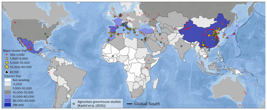
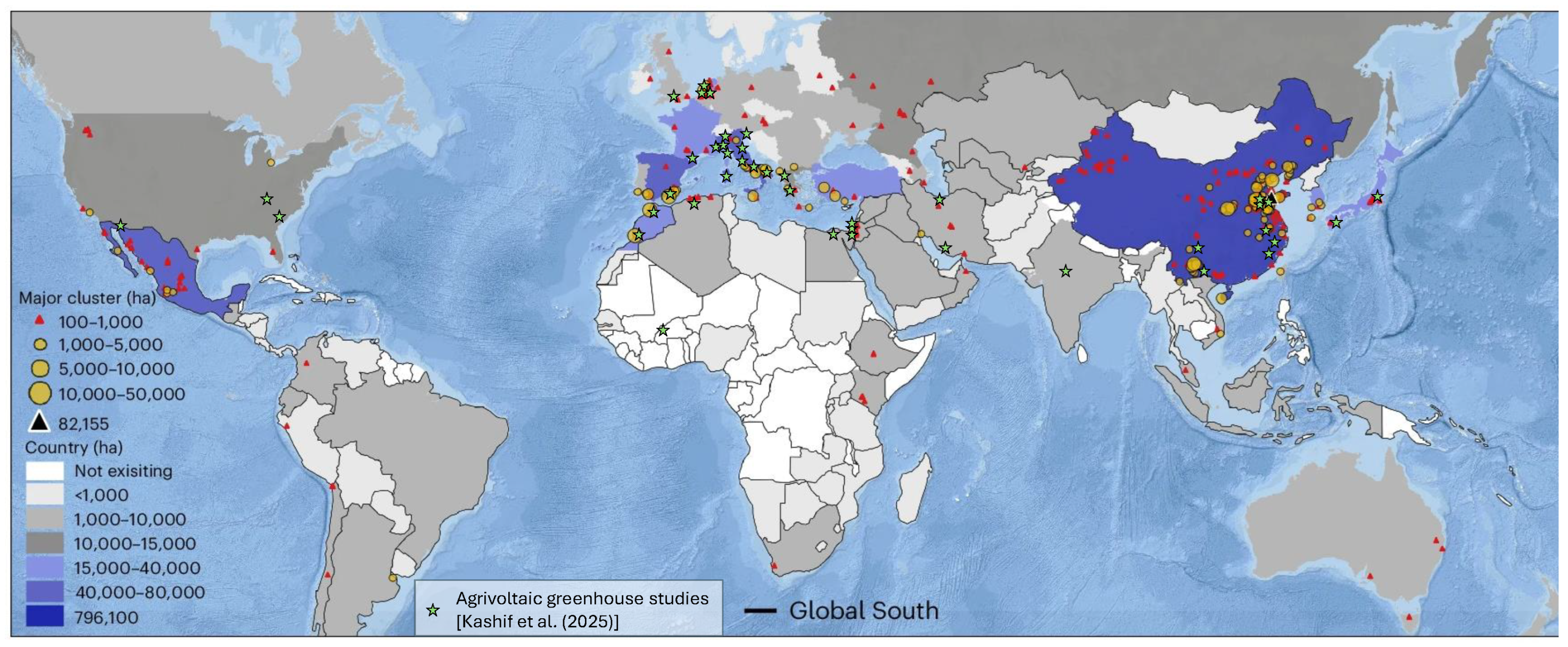
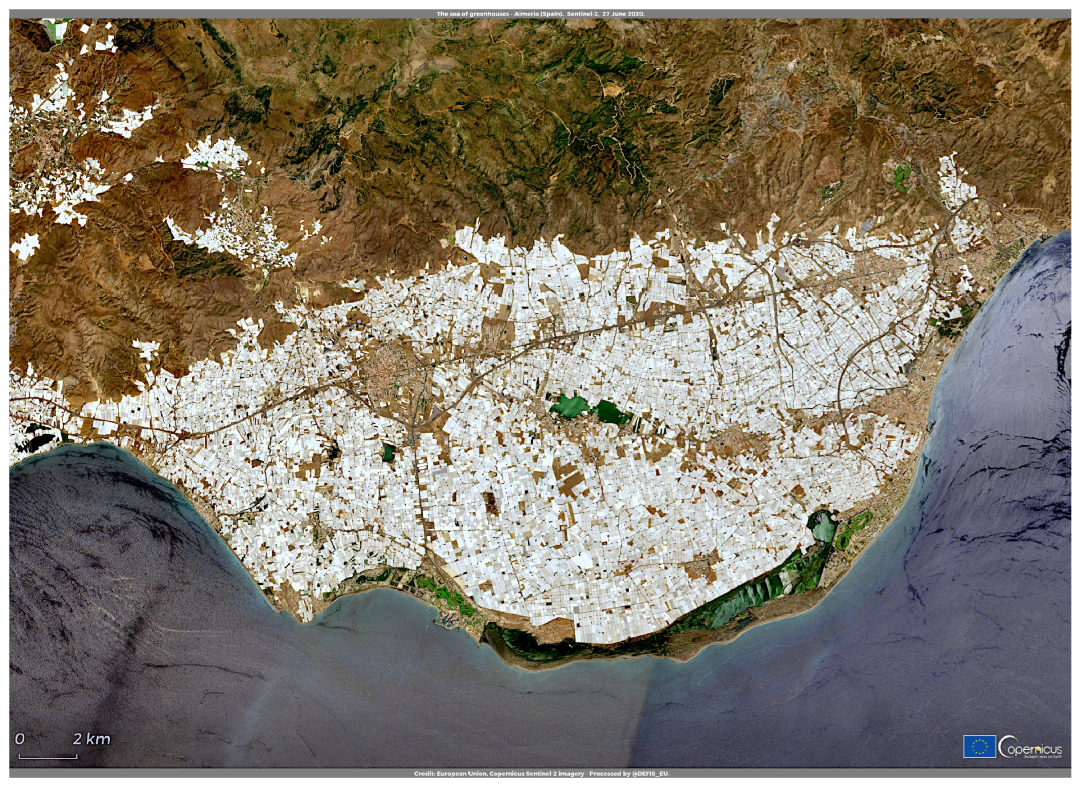
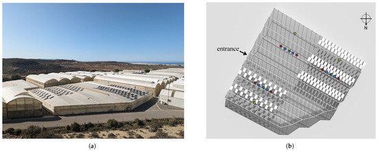
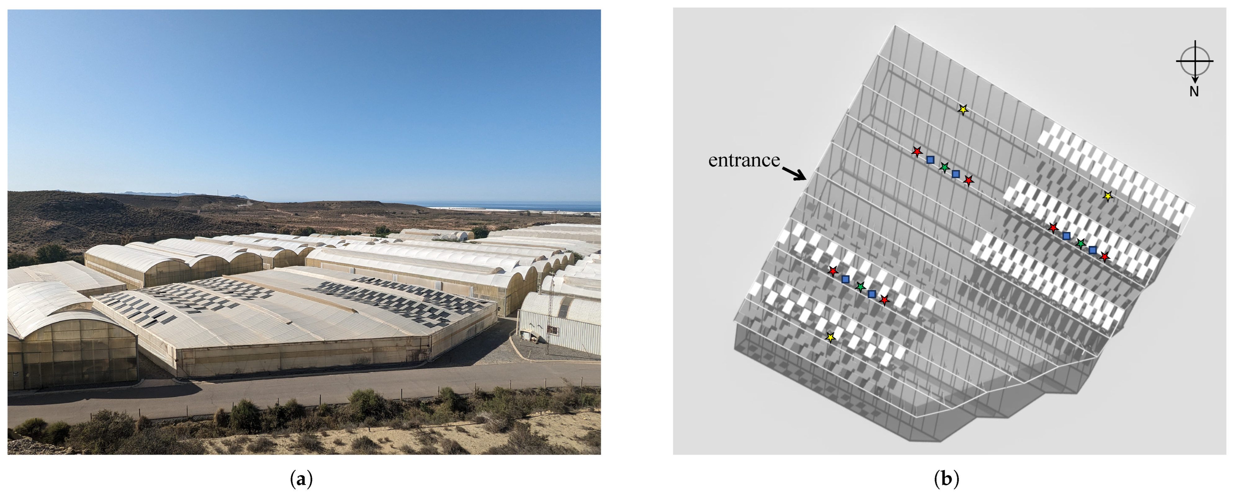
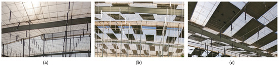
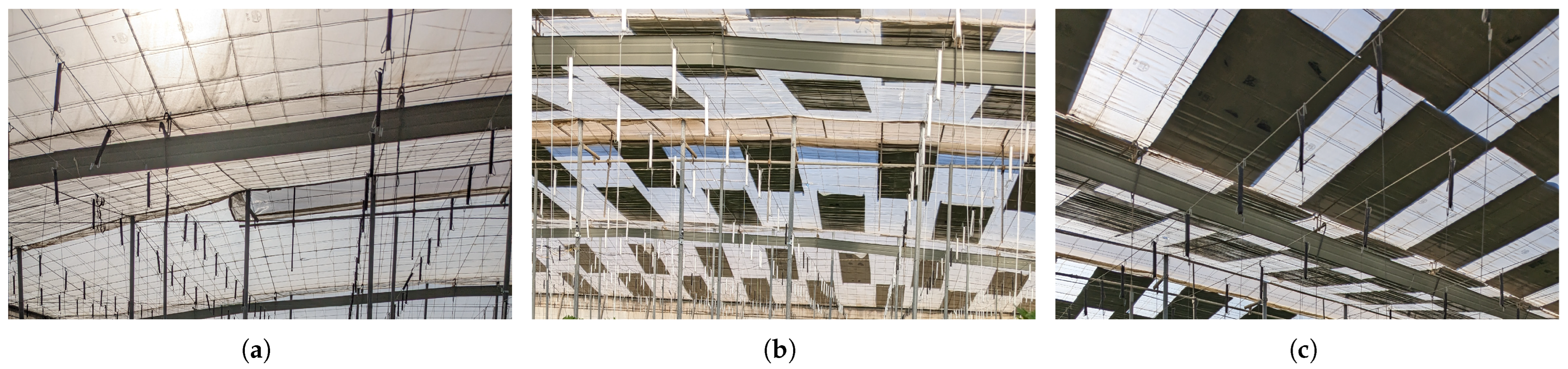
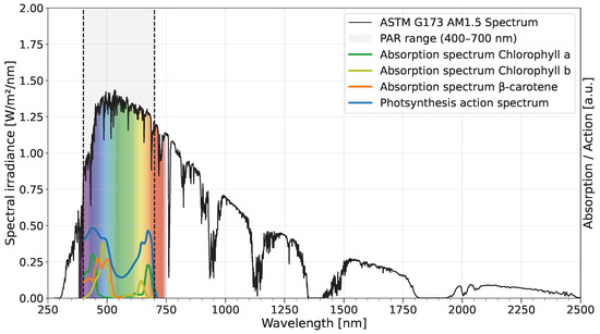
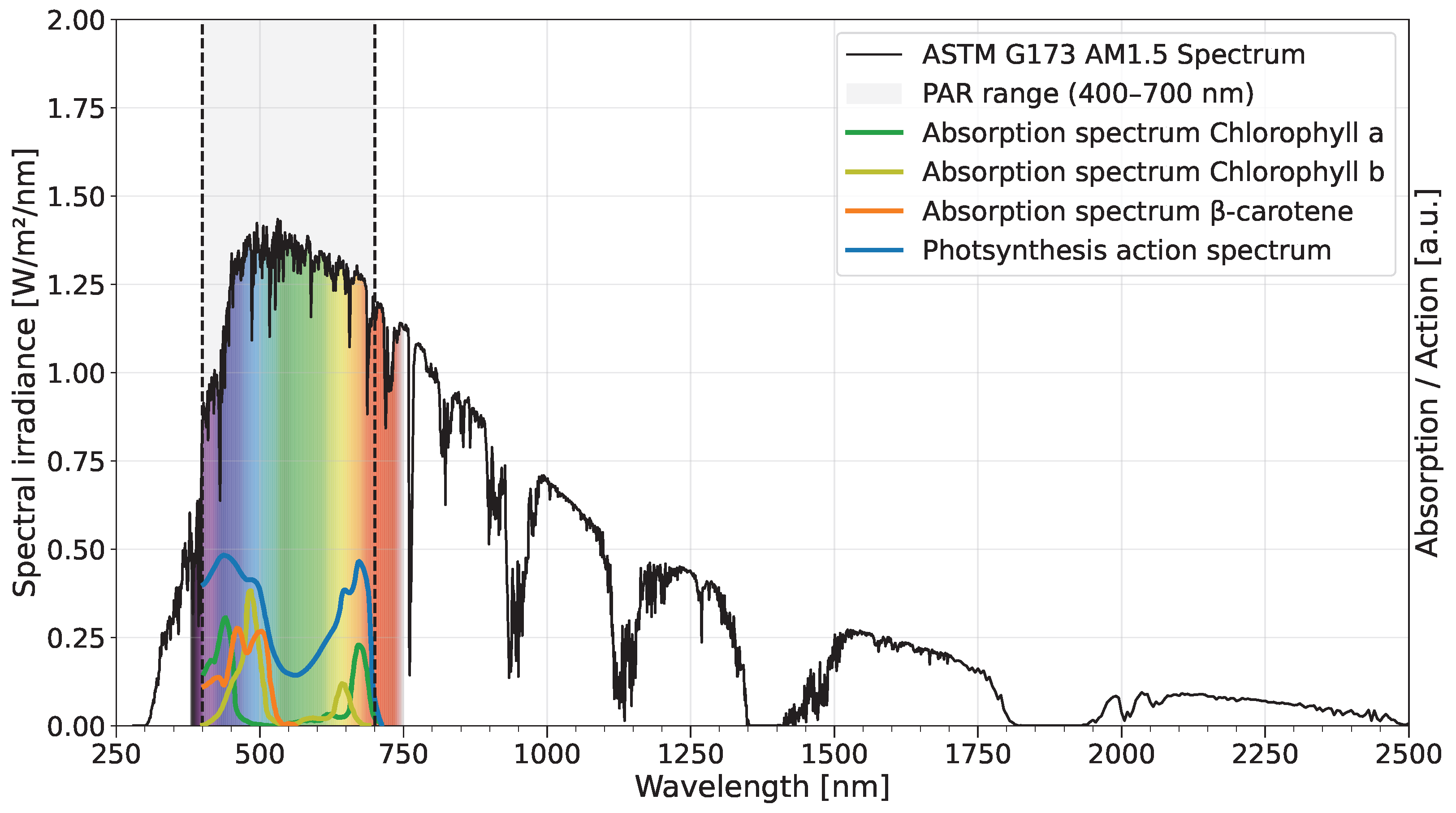
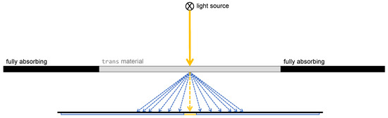
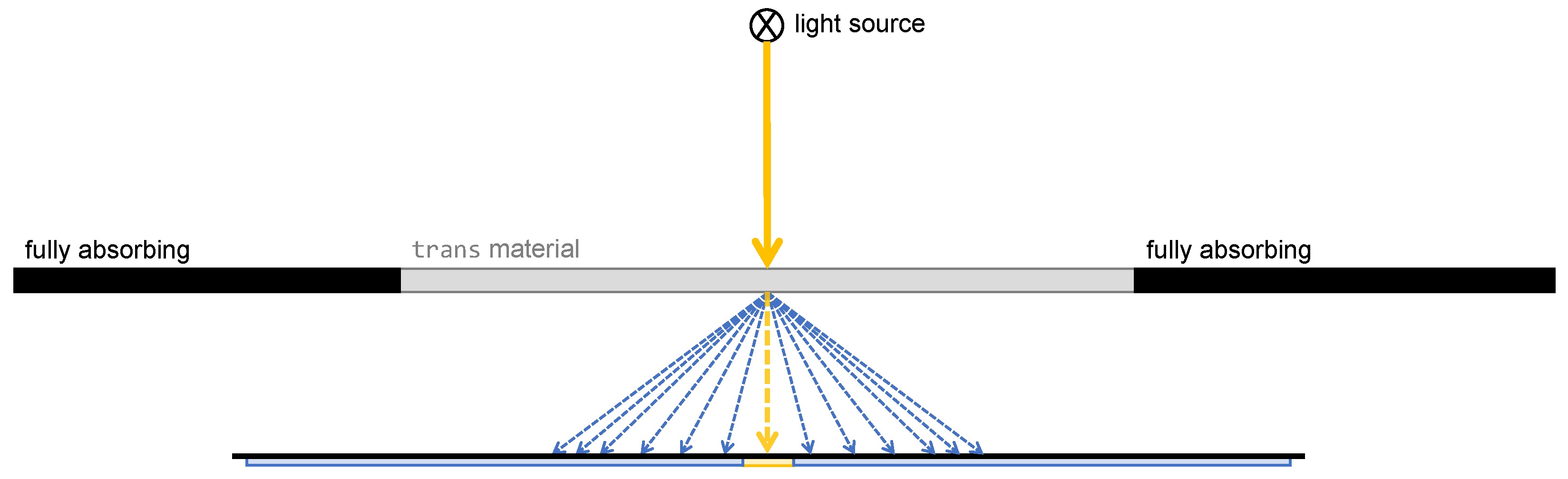
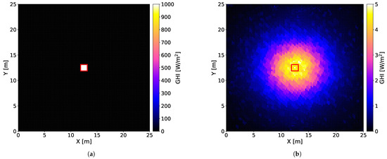
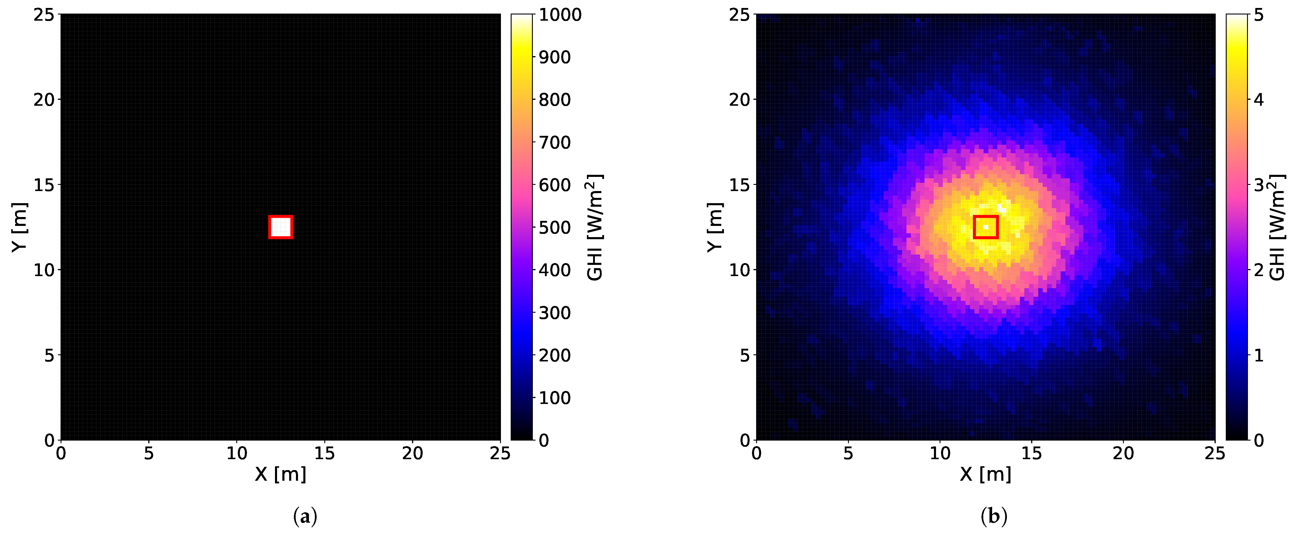
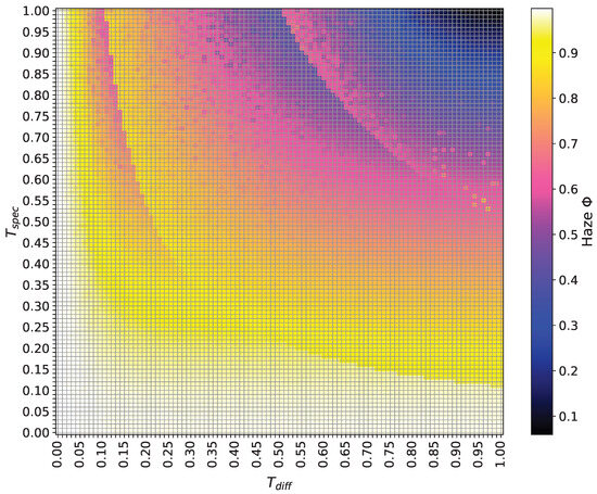
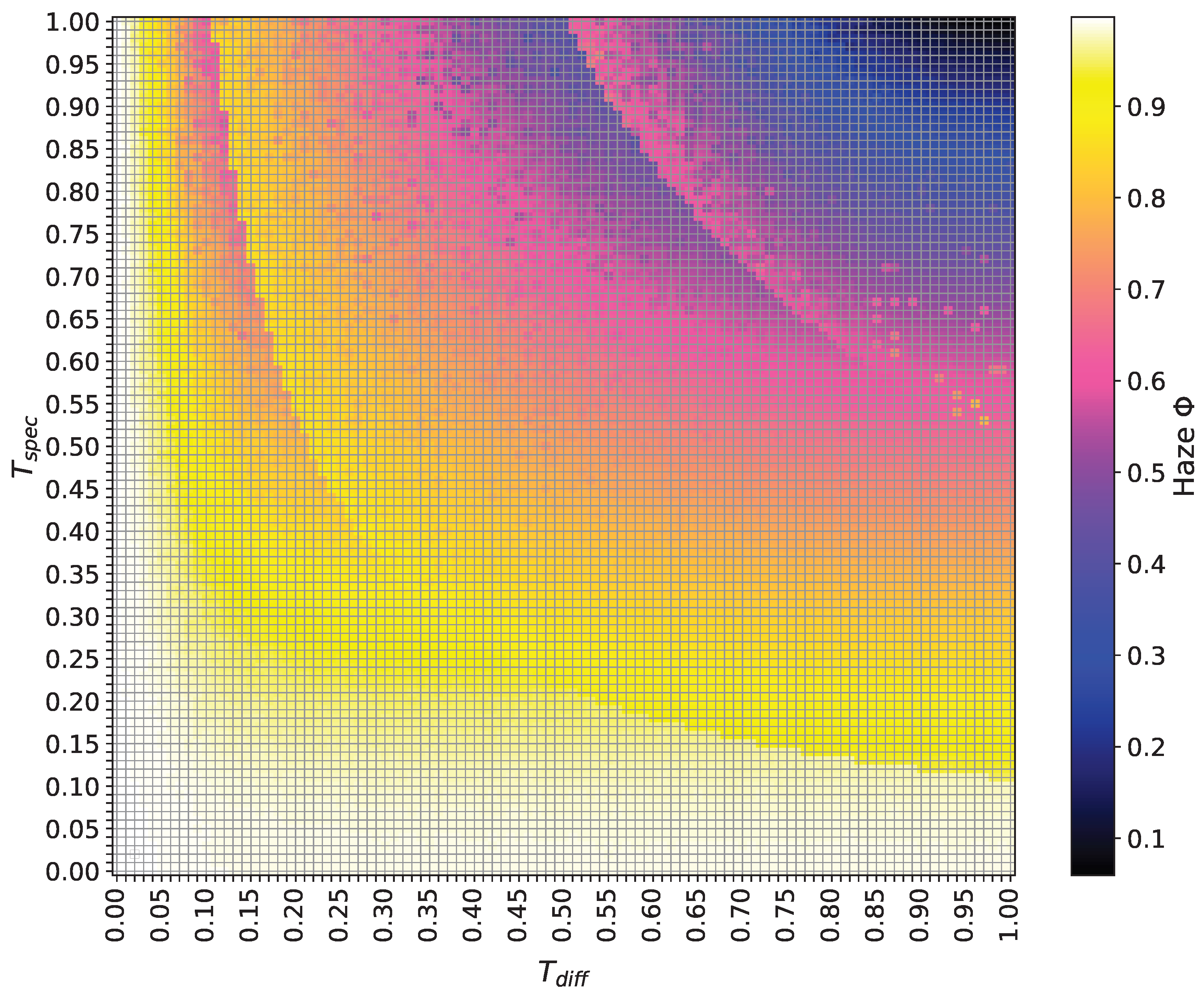
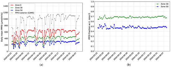
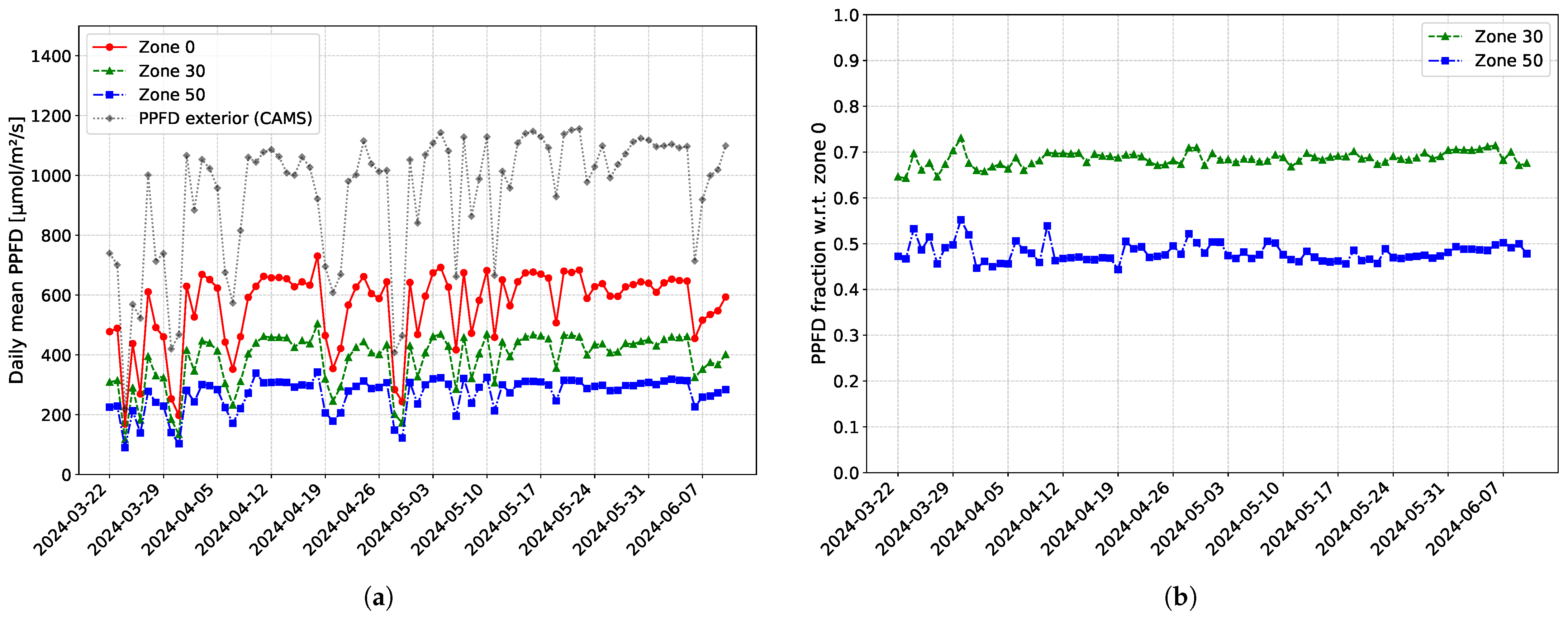
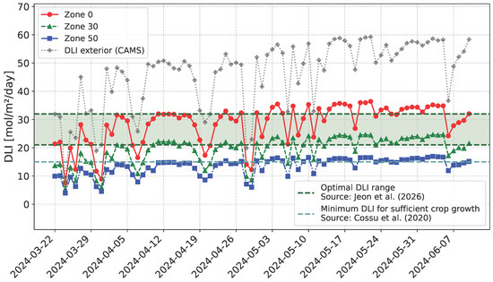
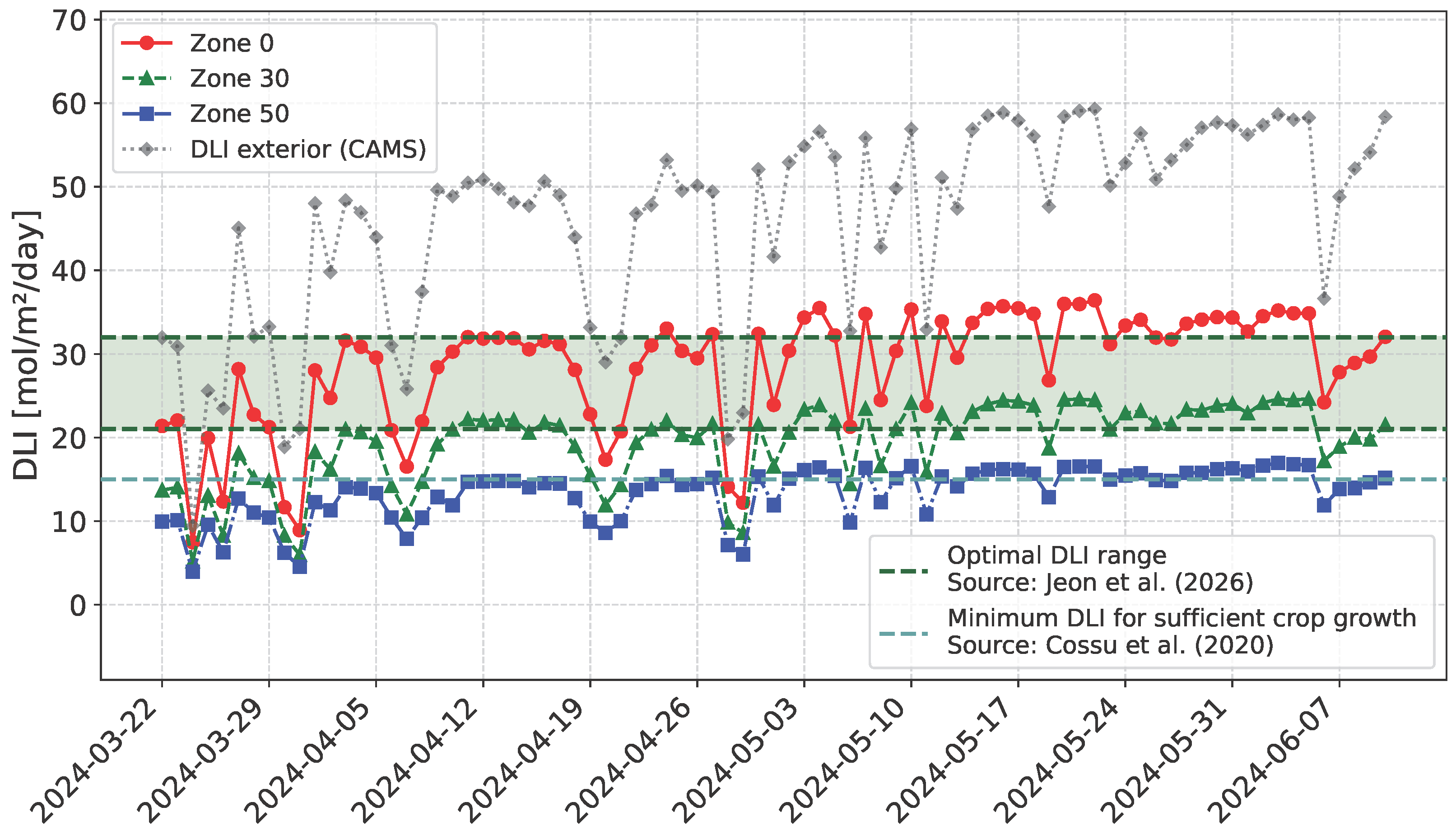
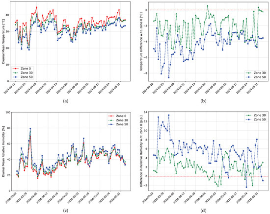
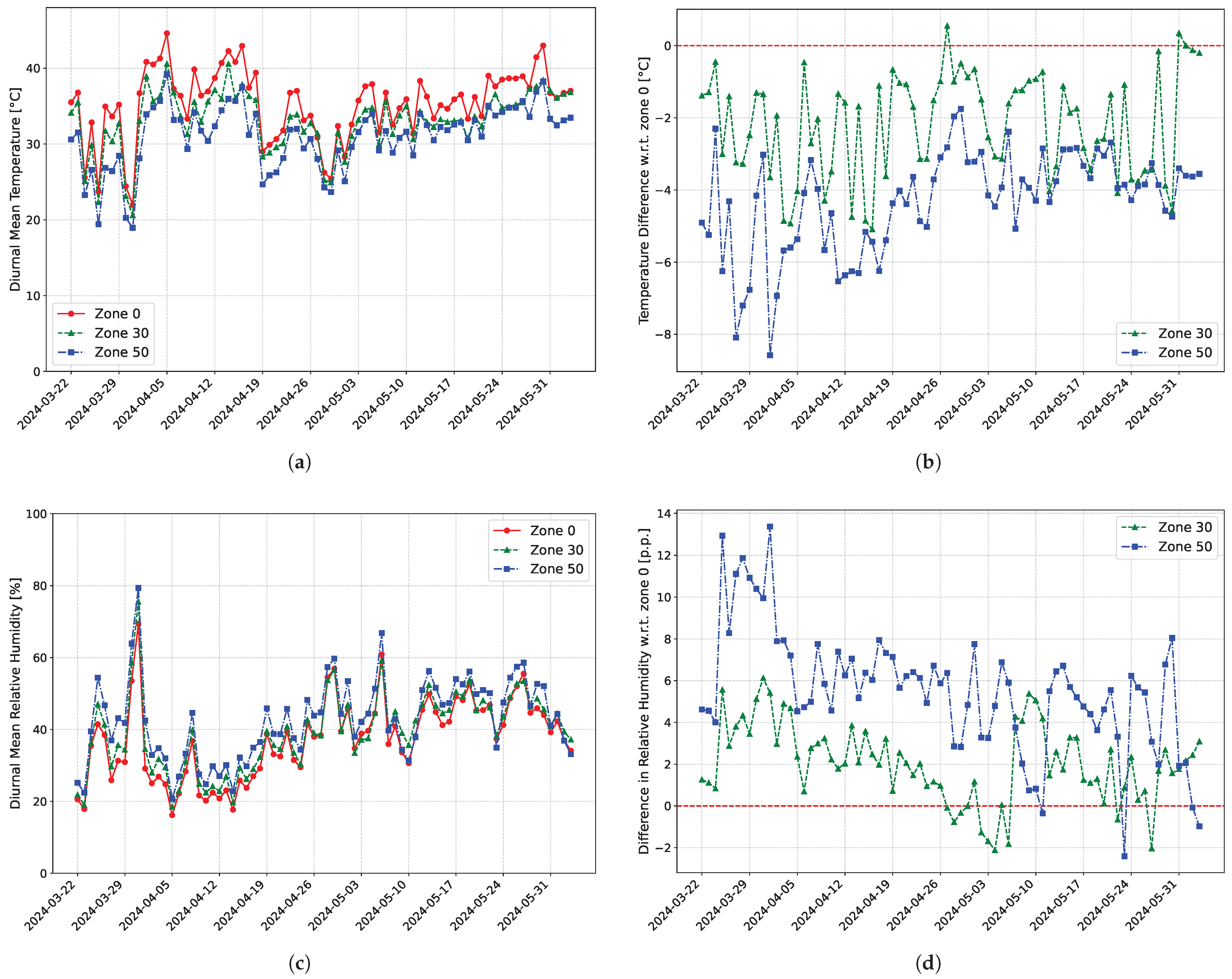
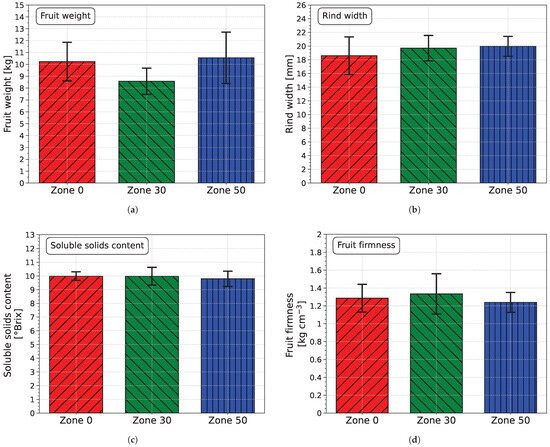
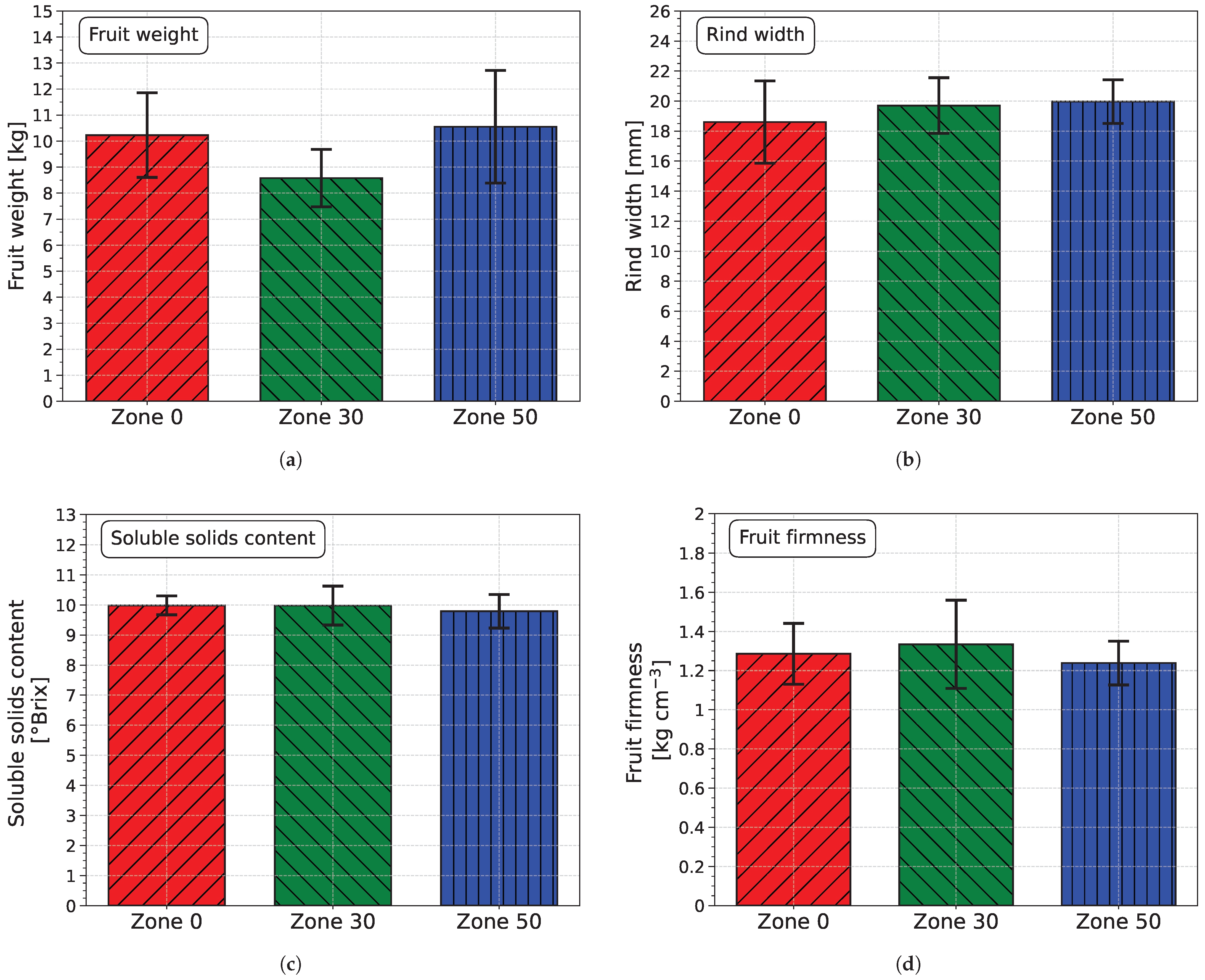
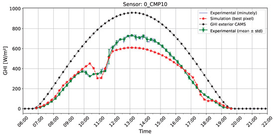
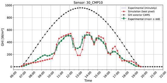
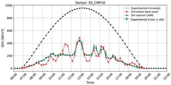
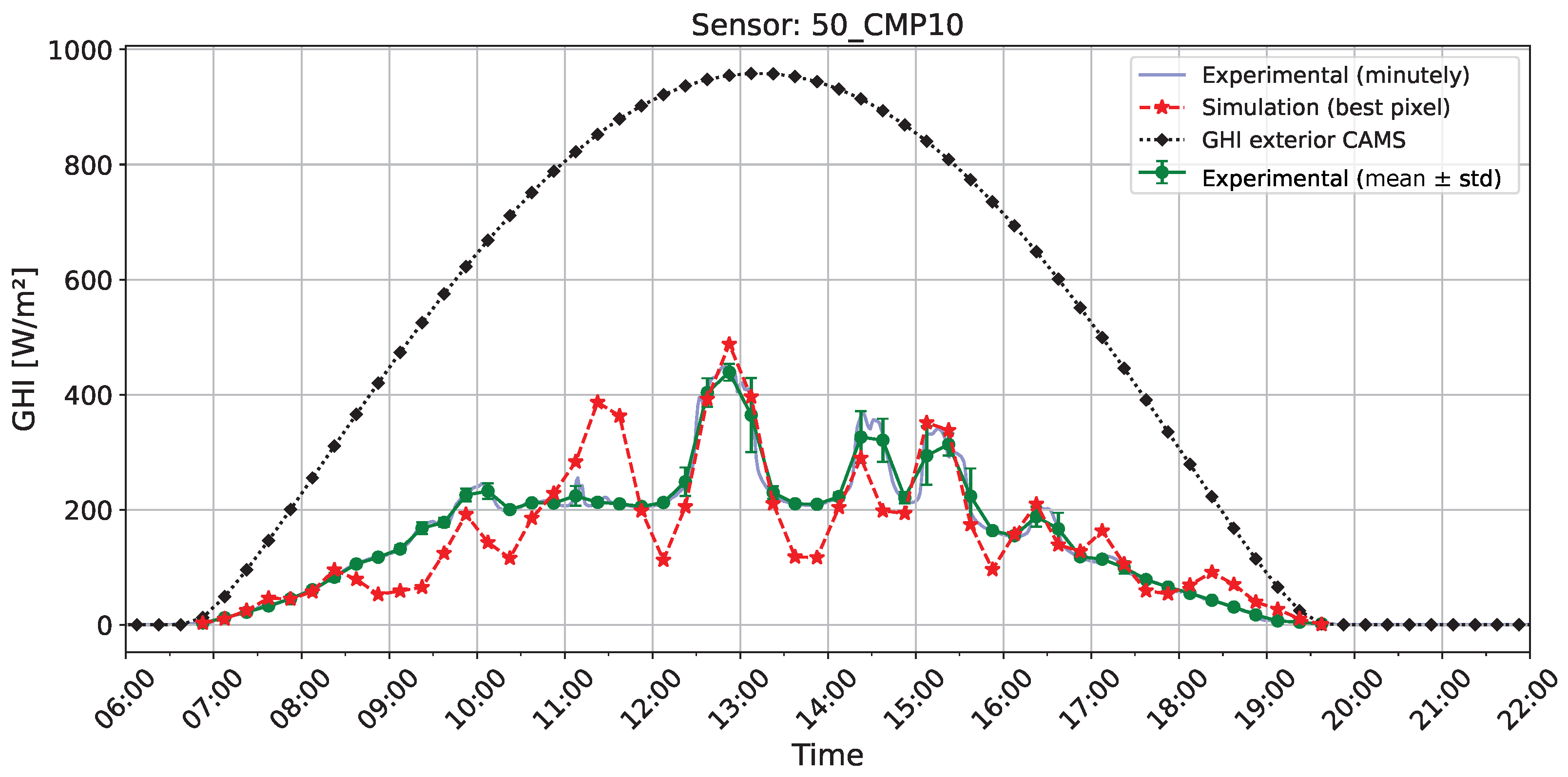
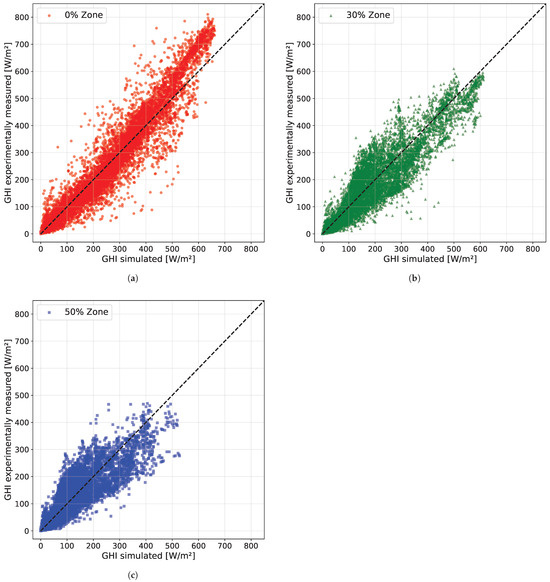
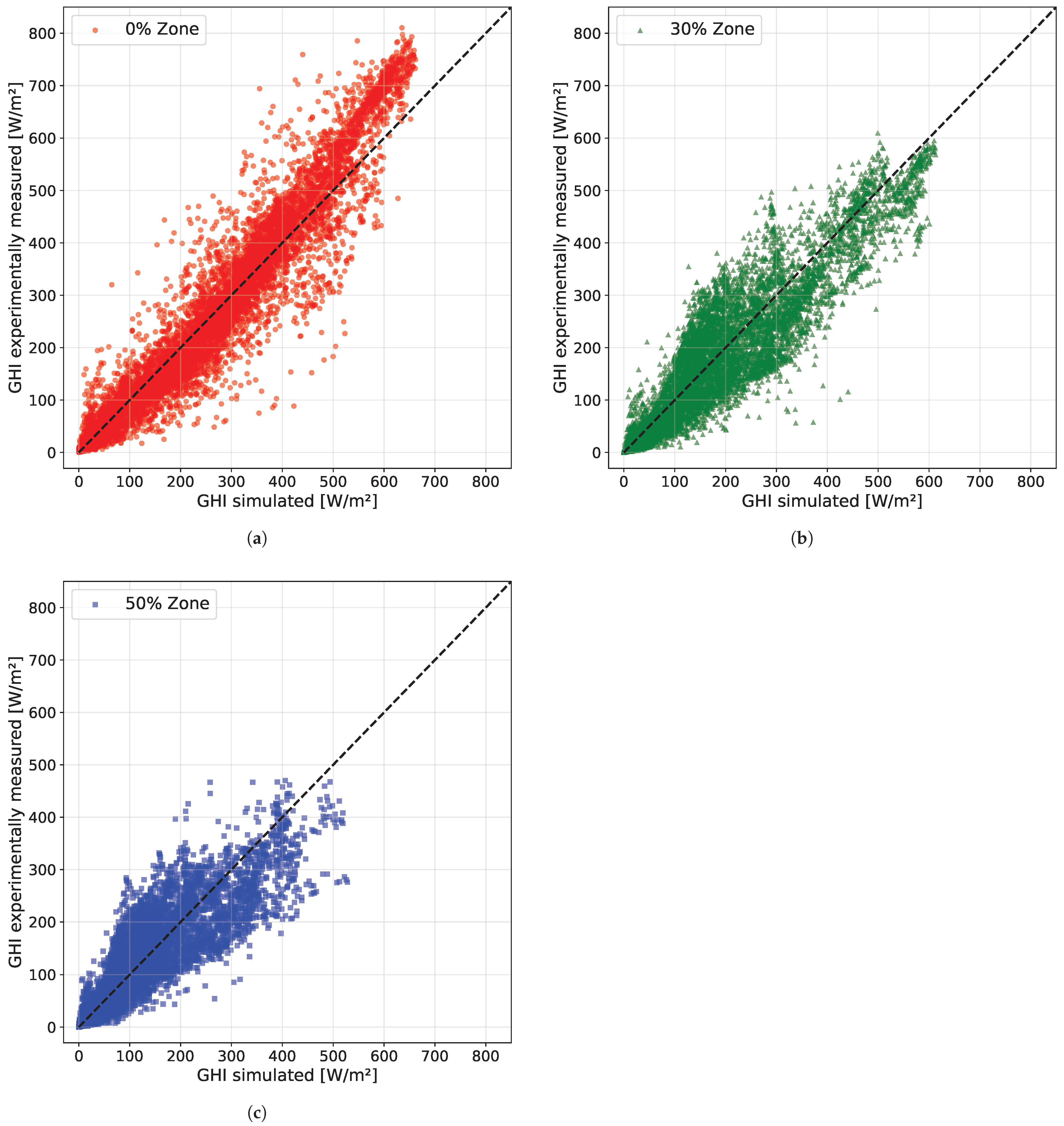
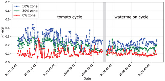
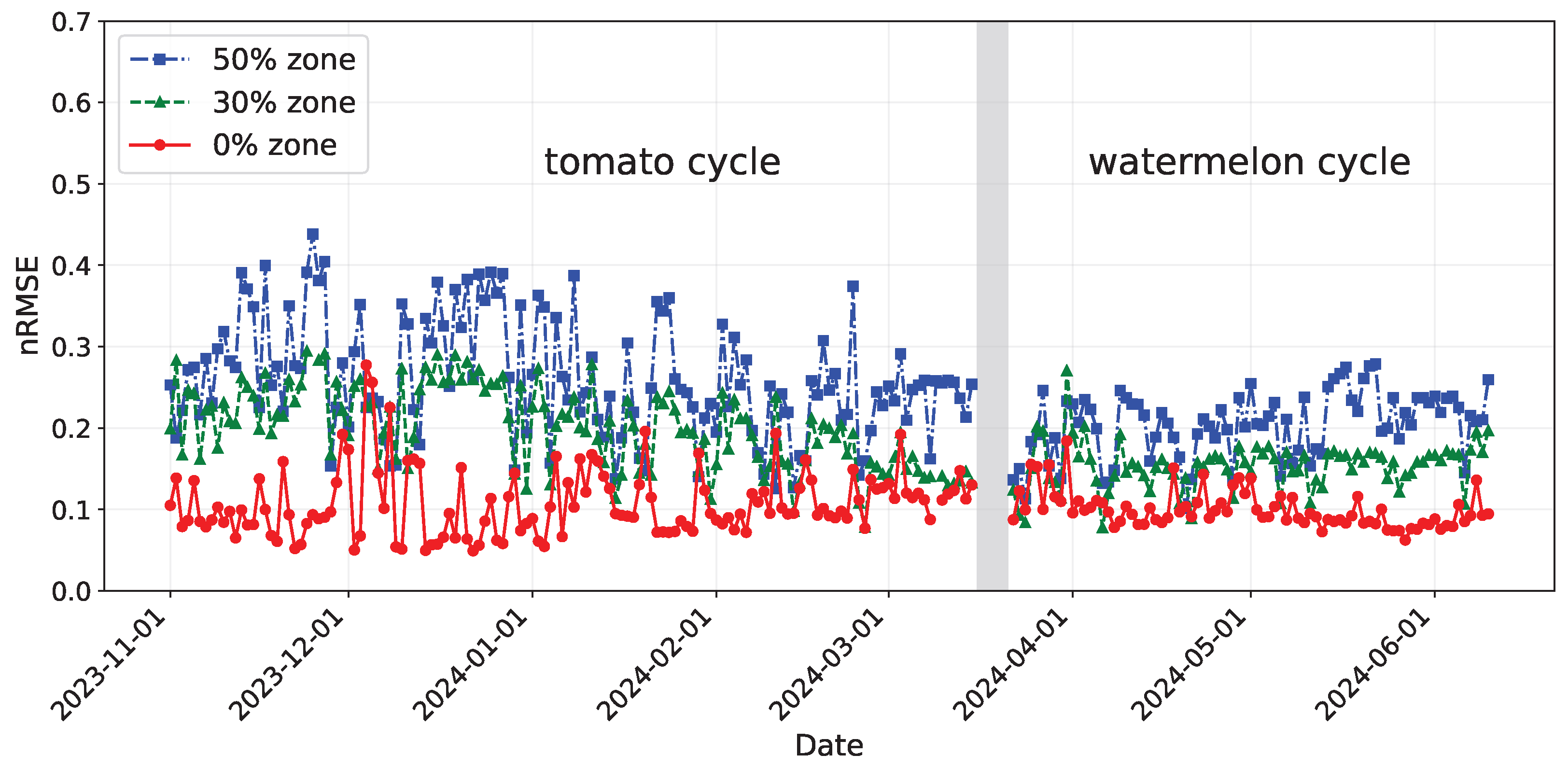

Disclaimer/Publisher’s Note: The statements, opinions and data contained in all publications are solely those of the individual author(s) and contributor(s) and not of MDPI and/or the editor(s). MDPI and/or the editor(s) disclaim responsibility for any injury to people or property resulting from any ideas, methods, instructions or products referred to in the content. |
© 2026 by the authors. Licensee MDPI, Basel, Switzerland. This article is an open access article distributed under the terms and conditions of the Creative Commons Attribution (CC BY) license.