Does Machine Learning Improve Wind Power Forecasting? An Experimental Investigation

Highlights

What are the main findings?

• The performance benefits of machine learning are task-dependent. For wind speed correction, tree-based ensemble and gradient boosting methods yield superior performance across all four feature configurations. For wind power forecasting, deep learning architectures substantially and consistently outperform traditional machine learning approaches on both datasets.
• No single model achieves universal superiority across different wind regimes. Attention-based models exhibit the strongest robustness against regime variations, whereas recurrent architectures are the most sensitive to wind regime shifts.

What are the implications of the main findings?

• Practitioners should implement task-oriented model selection. For wind speed correction, tree-based learners paired with deliberate feature engineering are recommended; for wind power forecasting, attention-based deep learning architectures are preferred. One should not assume that higher model complexity necessarily delivers better performance.
• Multi-site evaluation is indispensable for deriving reliable and generalizable model rankings. Studies relying solely on a single dataset may yield overly definitive and misleading conclusions.

Abstract

Accurate wind power forecasting is essential for the stable and economic operation of power systems with high renewable penetration. Although machine learning models have been widely adopted for this task, the assumption that greater model complexity invariably yields superior forecasting accuracy has received insufficient scrutiny. This paper presents a systematic experimental investigation that covers two complementary stages, i.e., wind speed correction and wind power forecasting. For wind speed correction, we compare 10 machine learning methods, including spanning linear, instance-based, and tree-based ensemble learners, under four newly proposed progressively enriched feature configurations. For wind power forecasting, we benchmark 20 methods spanning traditional machine learning, time-series deep learning, and Transformer-based architectures on two geographically distinct wind farms. Our results reveal a clear task-dependent pattern. In wind speed correction, tree-based ensemble methods, particularly gradient boosting variants, consistently dominate, and feature engineering contributes more to accuracy gains than model selection. In wind power forecasting, deep learning architectures substantially and consistently outperform traditional methods, with attention-based models generalizing the most robustly across regimes and recurrent networks proving to be the most sensitive to regime shifts. These findings provide actionable task-specific guidance for model selection in operational wind power forecasting systems.

1. Introduction

Wind energy has become a cornerstone of the global transition toward low-carbon energy systems. The inherent variability and intermittency of wind, however, pose significant challenges to power system operations, particularly with respect to balancing supply and demand, managing reserve capacity, and participating in electricity markets. Accurate wind power forecasting is therefore not merely an academic pursuit but a practical necessity for enabling high-penetration wind integration [1].

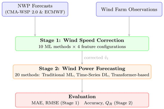
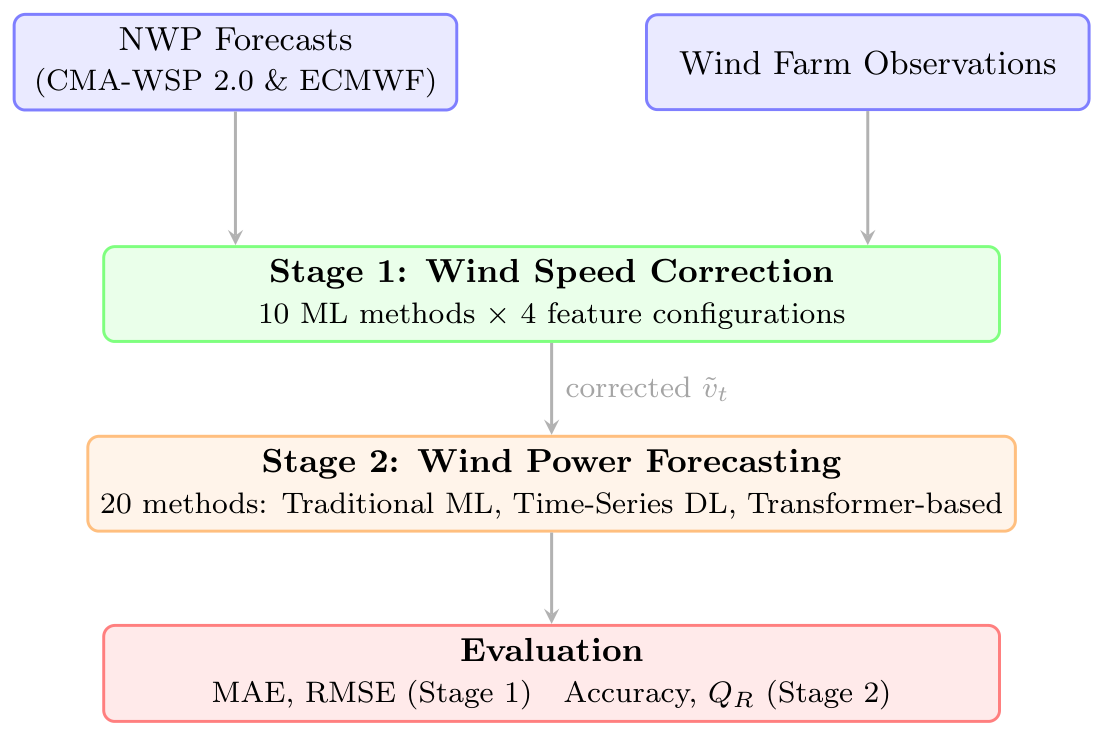
The wind power forecasting pipeline typically comprises two stages, as illustrated in Figure 1. In the first stage, numerical weather prediction (NWP) models provide forecasts of meteorological variables such as wind speed, wind direction, temperature, and air density at the wind farm location. NWP outputs are nevertheless known to contain systematic biases arising from coarse grid resolution, imperfect parameterization of physical processes, and local topographic effects [2]. A wind speed correction step is consequently applied to mitigate these errors, such as day-ahead correction via dynamic feature weighting of multi-source information [3], state-based correction with a modified hidden Markov model [4], downscaling correction in complex terrain [5], EOF-based correction of the leading bias modes [6], and regional bias correction [7]. In the second stage, the corrected meteorological variables serve as inputs to a power forecasting model that maps them to wind power outputs [8]. This research includes the application of large pretrained time-series foundation models to wind power [9], ML-based short-term forecasting [10], deep neural network approaches [11], and modern forecasting technologies [8].

Figure 1. Overall framework of the two-stage wind power forecasting pipeline.

The rapid advancement of machine learning has profoundly influenced both stages of this pipeline. On the wind speed correction front, methods ranging from linear regression to tree-based ensembles have increasingly been adopted. On the power forecasting front, an even wider array of deep learning architectures have been explored, including long short-term memory (LSTM) [12], gated recurrent units (GRUs) [13], temporal convolutional networks (TCNs) [14], and Transformer [15], often with impressive reported results.

Despite this proliferation of increasingly sophisticated methods, a critical question remains insufficiently addressed: Does machine learning actually improve wind power forecasting relative to simpler well-tuned alternatives? There are several reasons to doubt an unqualified affirmative answer. First, several recent studies have reported that the performance differences among competing deep learning architectures are surprisingly small. For instance, Zhang et al. [15] found that LSTM, GRU, TCN, and Transformer all achieved nearly identical mean absolute errors within a narrow range. Second, in the domain of wind speed correction, traditional machine learning methods such as random forest (RF) and XGBoost have been shown to match or exceed deep learning performance in multiple studies [16,17]. Winter et al. [18] further observed that varying neural network architectures had only a minor impact on forecast bias correction performance, suggesting that architectural complexity may matter less than data quality and feature engineering. Third, and most fundamentally, the relative efficacy of model families appears to be task-dependent rather than universal. The tabular feature-driven nature of wind speed correction may favor different inductive biases than the sequential temporally correlated dynamics of power generation, yet most existing studies evaluate only one of these stages in isolation. Beyond wind forecasting, machine learning techniques have demonstrated promising performance across broader renewable energy research domains. For instance, mechanistic machine learning approaches that integrate lignocellulosic structure, thermal severity, and multi-objective optimization have enabled data-driven optimization of biomass pyrolysis for enhanced organic bio-oil yield [19]. In the field of solar photovoltaic energy, hybrid frameworks combining machine learning with PVLib have been developed to optimize monthly PV tilt angles and improve energy yield under diverse global climate conditions [20]. Such cross-domain achievements highlight that the selection and complexity of machine learning models constitute a critical research topic in renewable energy, which motivates the present investigation focusing specifically on wind power forecasting pipelines.

Motivated by these observations, this paper presents a systematic experimental investigation designed to rigorously evaluate whether machine learning improves wind power forecasting. We decompose this overarching question into two concrete sub-questions:

• RQ1: How do different machine learning methods compare for NWP wind speed error correction?
• RQ2: How do deep learning and traditional machine learning methods compare for wind power forecasting?

To answer these questions, we conduct extensive experiments on real-world datasets collected from operational wind farms. Our contributions are summarized as follows:

• We provide a comprehensive head-to-head comparison of more than 20 machine learning methods across both critical tasks of the wind power forecasting pipeline.
• For wind speed correction, we systematically compare linear regression, ridge regression, k-nearest neighbors (KNN), decision tree, extra trees, gradient boosting decision tree (GBDT), random forest, XGBoost, CatBoost, and LightGBM, revealing that tree-based ensemble methods consistently outperform linear and instance-based alternatives in terms of both accuracy and robustness.
• For wind power forecasting, we benchmark 20 methods spanning three families, including traditional machine learning, time-series deep learning, and Transformer-based architectures, on two geographically and climatologically distinct wind farms, finding that deep learning models consistently and substantially outperform traditional machine learning methods.
• We conduct systematic multi-stage feature engineering for wind speed correction and devise four progressively enriched feature configurations that hierarchically integrate surface meteorological variables, vertical isobaric atmospheric profiles, and multi-NWP ensemble outputs, quantifying the relative contributions of feature engineering and model selection.

The remainder of this paper is organized as follows. Section 2 reviews the related work on wind speed correction and wind power forecasting. Section 3 details the datasets. Section 4 describes the methodological framework and the models evaluated in our experiments. Section 5 presents and discusses the experimental results. Section 6 concludes the paper with a summary of the findings and directions for future work.

2. Related Work

2.1. Wind Speed Correction

The accuracy of wind power forecasts is fundamentally constrained by the quality of the input wind speed forecasts. NWP models, despite their physical sophistication, produce wind speed predictions that contain systematic biases arising from multiple sources, including limited horizontal resolution that cannot resolve local terrain effects, simplified boundary-layer parameterizations, and errors in the initial conditions [2]. Wind speed correction, also referred to as model output statistics (MOS) or post-processing, aims to statistically remove these biases.

Early approaches to wind speed correction relied on classical statistical methods. The MOS approach [21] applies linear regression to establish a relationship between NWP outputs and observations. While simple and interpretable, linear MOS fails to capture the nonlinear structure of NWP errors. Subsequent improvements include autoregressive integrated moving average (ARIMA) models and Kalman filtering techniques, which exploit the temporal structure of forecast errors [2].

The past decade has witnessed a shift toward machine learning-based correction methods, with tree-based ensemble methods proving to be particularly effective. Sun et al. [22] compared LASSO regression, RF, and deep learning for correcting ECMWF 10 m wind speed forecasts over northern China, finding that all three machine learning methods outperformed traditional MOS, with RF achieving the best overall performance. Fang et al. [23] proposed the WSFBC-XGB model for wind speed bias correction in the Hangzhou area, achieving notable RMSE reduction relative to a raw NWP output. Ren et al. [24] applied an XGBoost-based multi-model ensemble to complex terrain, reducing 10 m wind speed errors. More recently, Zeng et al. [17] demonstrated that a stacking ensemble of LightGBM, CatBoost, and XGBoost, augmented with spatial information from neighboring grid points, improved wind speed forecast accuracy.

2.2. Wind Power Forecasting

The application of deep learning to wind power forecasting has been an active area of research. Early deep learning approaches for wind power forecasting primarily employed recurrent neural networks (RNNs) and their variants. LSTM networks, designed to address the vanishing gradient problem of vanilla RNNs, became the de facto standard. Wang et al. [12] proposed C-LSTM, which embeds an adaptive wind speed calibration mechanism within the LSTM framework, demonstrating consistent improvements over standard LSTM across several wind turbines. BiLSTM, which processes sequences in both forward and backward directions, has been shown to further improve accuracy [25].

Convolutional neural networks, originally designed for image processing, have been adapted for time-series forecasting by employing one-dimensional convolutions that slide along the temporal dimension. TCNs, which use dilated causal convolutions, offer an alternative to recurrent architectures with the advantages of parallel computation and stable gradients. Chen et al. [14] proposed a TCN–FAM–Transformer model that demonstrated superior performance under peak fluctuation scenarios.

The Transformer architecture, introduced by Vaswani et al. [26], has increasingly been adopted for wind power forecasting. Its multi-head self-attention mechanism enables the model to capture long-range dependencies more effectively than recurrent architectures. Wang et al. [27] proposed GCNInformer, combining graph convolutional networks with the Informer, which significantly outperformed LSTM, RNN, Transformer, and the vanilla Informer by incorporating spatial correlations among wind turbines. The Fast-Powerformer [28] achieved MSE reduction relative to the standard Transformer baseline for mid-term forecasting. More recently, large time-series models have been explored as foundation forecasters for wind power [9], broadening the spectrum of available architectures.

2.3. Comparative Studies and Benchmarking Efforts

Several recent studies have conducted systematic comparisons across multiple methods, providing valuable insights for the field. Elmousalami et al. [29] evaluated a wide range of machine learning and deep learning algorithms for wind speed and power prediction. Liu et al. [1] provided a comprehensive survey of data-driven wind power prediction methods, covering spatial scales from individual turbines to regional wind farms, and identified attention mechanisms and Transformer variants as the most promising research direction.

Despite these efforts, existing comparative studies frequently suffer from one or more limitations: evaluating methods on a single dataset or geographic location, using inconsistent evaluation protocols across methods, or focusing on only one stage of the forecasting pipeline. Our work addresses these gaps by conducting a unified multi-site evaluation of both wind speed correction and wind power forecasting under consistent experimental conditions.

3. Datasets

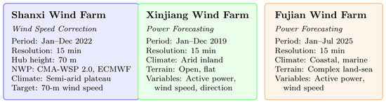
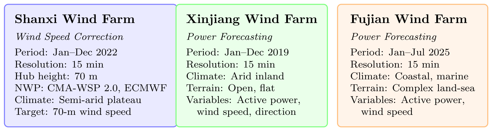
To ensure the generalizability of our findings, we employ three real-world datasets collected from geographically and climatologically distinct wind farms in China, as summarized in Table 1 and illustrated in Figure 2, i.e., wind speed correction on the Shanxi and wind power forecasting on the Xinjiang and Fujian datasets. This decoupled design allows each stage to be evaluated under the most appropriate data conditions for its task while retaining the conceptual coherence of the overall pipeline.

Table 1. Summary of the three datasets used in this study.

Dataset	Period	Resolution	Task
Shanxi	January–December 2022	15 min	Wind speed correction
Xinjiang	January–December 2019	15 min	Power forecasting
Fujian	January–July 2025	15 min	Power forecasting

Figure 2. Geographic and climatological overview of the three wind farm datasets.

3.1. Wind Speed Correction Dataset

The wind speed correction experiments are conducted using forecasts from CMA-WSP 2.0 and ECMWF, with observations from a wind farm in Shanxi, China. The wind farm meteorological mast provides 70 m hub-height wind speed observations at 15 min intervals, covering the period from January to December 2022.

From CMA-WSP 2.0, we obtain forecasts at 9 km spatial resolution and 15 min temporal resolution, with lead times up to 72 h. The variables include

• Surface meteorology: 2 m temperature, 2 m specific humidity, 2 m relative humidity, skin temperature, boundary-layer height, and surface pressure.
• Near-surface wind fields: Wind speed and direction at 10 m, 30 m, 50 m, 70 m, 80 m, 100 m, and 120 m above ground level.
• Radiation and energy: Surface downward shortwave radiation, normal shortwave radiation, surface downward direct radiation, clear-sky surface downward direct radiation, surface diffuse radiation, surface downward longwave radiation, and albedo.
• Convective parameters: Convective available potential energy (CAPE) and convective inhibition (CIN).
• Pressure-level variables: Wind speed, wind direction, vertical velocity ($\omega$), temperature, geopotential height, relative humidity, and specific humidity at pressure levels 200 hPa, 500 hPa, 700 hPa, 850 hPa, 925 hPa, and 1000 hPa.

The corresponding ECMWF forecast variables at matching pressure and surface levels are also included. The target variable for correction is the observed 70 m wind speed from the meteorological mast.

3.2. Wind Power Forecasting Datasets

For wind power forecasting, we employ two geographically distinct datasets to ensure that our findings are not biased toward a single climate regime or terrain type.

Dataset I: Xinjiang Wind Farm. The first dataset originates from a wind farm in Xinjiang, China, covering the full year of 2019 at 15 min intervals. The dataset records the wind farm’s active power output together with meteorological variables including wind speed and wind direction.

Dataset II: Fujian Wind Farm. The second dataset covers Fujian, China, from 1 January to 14 July 2025, at 15 min intervals. The dataset includes timestamped short-term reported power and short-term reported wind speed.

The use of two geographically distant wind farms is a deliberate experimental design choice. It mitigates the risk of dataset-specific overfitting and ensures that any performance ranking among the deep learning architectures reflects genuine modeling capability rather than idiosyncrasies of a single location. The climatological, topographical, and seasonal differences between the two sites provide a robust testbed for assessing model consistency.

4. Methodology

4.1. Problem Formulation

We formulate the wind power forecasting problem as a two-stage pipeline. In the first stage (wind speed correction), we aim to learn a mapping $f_{\mathrm{corr}}$ that corrects the NWP-predicted wind speed ${\widehat{v}}_t$ to better approximate the observed wind speed $v_t$,

$${\tilde{v}}_t=f_{\mathrm{corr}}({\widehat{v}}_t,{\mathbf{x}}_t^{\mathrm{NWP}}),$$

(1)

where ${\mathbf{x}}_t^{\mathrm{NWP}}$ denotes auxiliary NWP variables (e.g., wind direction, temperature, pressure, and humidity) at time t, and ${\tilde{v}}_t$ is the corrected wind speed.

In the second stage (wind power forecasting), we learn a mapping $f_{\mathrm{power}}$ from the corrected meteorological variables to wind power output $p_t$,

$${\widehat{p}}_t=f_{\mathrm{power}}({\tilde{v}}_t,{\mathbf{x}}_t^{\mathrm{other}}),$$

(2)

where ${\mathbf{x}}_t^{\mathrm{other}}$ may include additional features such as historical power output, wind direction, and air density.

For both tasks, we consider a multi-step-ahead forecasting setting. Given a look-back window of length $T_{\mathrm{in}}$, the model predicts the target variable for the next $T_{\mathrm{out}}$ time steps,

$${\mathbf{y}}_{t+1:t+T_{\mathrm{out}}}=F\left({\mathbf{X}}_{t-T_{\mathrm{in}}+1:t}\right),$$

(3)

where $\mathbf{X}$ denotes the input feature matrix and $\mathbf{y}$ denotes the target variable (corrected wind speed or wind power). We should note that these two tasks are complementary but independently evaluated.

4.2. Feature Engineering for Wind Speed Correction

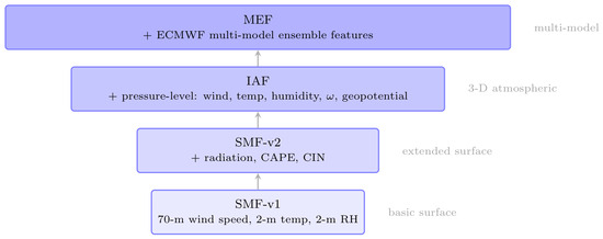
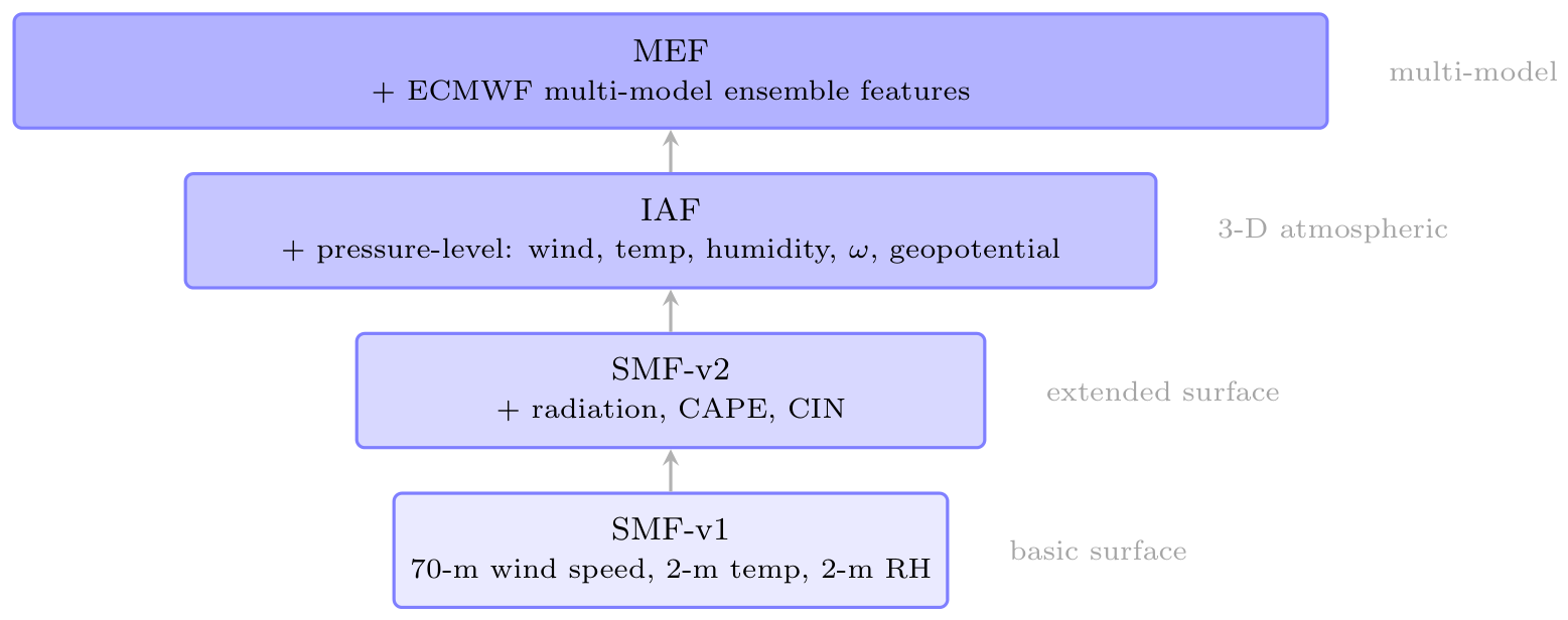
The design of input features is a critical factor that influences the effectiveness of data-driven wind speed correction. Rather than treating wind speed as an isolated variable, we exploit the well-established coupling relationships among meteorological variables to construct feature sets of increasing richness. We design four progressively enriched feature configurations, as summarized in Figure 3.

Figure 3. Hierarchical structure of the four feature engineering configurations.

4.2.1. Surface Meteorological Features (SMF-v1 and SMF-v2)

Wind speed does not exist in isolation but interacts with numerous other meteorological variables through well-understood physical mechanisms. Temperature directly influences air density and atmospheric dynamics, temperature changes alter vertical motion and wind field structure, while warm and cold advection, particularly during frontal passages, can cause significant wind speed variations. Relative humidity reflects the moisture content of the atmosphere and interacts with wind speed through boundary-layer turbulent exchange and precipitation processes. Changes in humidity can trigger evaporative cooling or condensational heating, further modulating local wind speed.

Building on these physical considerations, we define two surface-level feature configurations. SMF-v1 uses only the three most basic surface variables, i.e., 70 m wind speed, 2 m temperature, and 2 m relative humidity. SMF-v2 extends SMF-v1 by incorporating additional atmospheric parameters that capture higher-order physical processes, including surface shortwave and longwave radiation, CAPE, and CIN.

4.2.2. Isobaric Atmospheric Features (IAFs)

Beyond surface observations, the three-dimensional structure of the atmosphere carries essential information for wind speed prediction. The coupling between upper-level and lower-level atmospheric states is governed by fundamental dynamical and thermodynamic processes. At different pressure levels, wind speed and direction profiles reflect the combined effects of the pressure gradient force, the Coriolis force, and thermal processes.

We therefore construct the IAF configuration by augmenting SMF-v2 with upper-air variables at multiple isobaric levels (e.g., 500 hPa, 700 hPa, 850 hPa, and 925 hPa), including wind speed and direction, temperature, relative and specific humidity, vertical velocity, and geopotential height. By incorporating these multi-level features, the model gains a three-dimensional perspective on the atmospheric state, enabling it to capture vertical coupling mechanisms that surface observations alone cannot resolve.

4.2.3. Multi-Model Ensemble Features (MEFs)

Individual NWP systems each carry inherent biases arising from their respective model physics, grid resolutions, and data assimilation strategies. Combining forecasts from multiple NWP sources can reduce these systematic errors through diversity-driven error cancellation. We construct the MEF configuration by merging the CMA-WSP 2.0 and ECMWF forecast products. The MEF configuration concatenates the full IAF feature vectors from both systems, effectively doubling the input dimensionality. This allows the correction model to learn the systematic differences between the two NWP systems and exploit their complementary information content.

4.3. Wind Speed Correction Methods

For wind speed correction, we evaluate 10 methods spanning linear regression (LR), ridge regression, decision tree (DT), k-nearest neighbors (KNN), random forest (RF), extra trees and four gradient boosting variants, GBDT, XGBoost, CatBoost, and LightGBM.

4.4. Wind Power Forecasting Methods

For wind power forecasting, we benchmark 20 machine learning methods organized into three families. The traditional machine learning family comprises seven methods including extra trees, SVR, random forest, ridge regression, LightGBM, XGBoost, and GBDT. The time-series deep learning family comprises seven models, i.e., LSTM and GRU, TCN, DLinear, LightTS, TimeMixer, and TSMixer. The Transformer-based family comprises six attention-based architectures including Autoformer, Informer, FEDFormer, Crossformer, iTransformer, and Transformer–BiLSTM.

4.5. Experimental Setup

All the experiments follow a consistent evaluation protocol. For each dataset, we adopt a chronological split to preserve the temporal ordering of the data: the first 70% of samples for training, the next 10% for validation, and the final 20% for testing. This approach prevents data leakage and simulates real-world operational deployment conditions. The pseudocode can be found in Algorithm 1.

For wind speed correction, the input window $T_{\mathrm{in}}$ is set to 1. For wind power forecasting, the model input comprises the multivariate history of wind speed over a look-back window of $T_{\mathrm{in}}=96$ (24 h at 15 min resolution), and the prediction horizon is $T_{\mathrm{out}}=96$. Traditional machine learning methods are implemented using scikit-learn, and the default settings were used. Specifically, the $l_2$ regularizer for ridge regression is $\alpha =1.0$, the number of neighbors of KNN is 5, the number of estimators for all the tree-based methods is set to be 100, and the learning rates for GBDT, XGBoost, LightGBM and CatBoost are $0.1$, $0.5$, $0.1$ and $auto$. We adopted a direct multi-output strategy for all the traditional machine learning models. Deep learning models are implemented in PyTorch V2.10.0. A uniform reproducible protocol was adopted for all the models to ensure a fair comparison, i.e., using the Adam optimizer with an initial learning rate of $1\times {10}^{-3}$, which was decayed by a factor of 0.5 when the validation loss plateaued. The mean squared error (MSE) was adopted as the loss function, the batch size was set to 256, and the maximum training epochs were limited to 100. An early-stopping strategy was implemented with a patience of 10 epochs monitored on the validation loss, a dropout rate of 0.1 was applied for regularization, and the hidden dimension was configured as 256.

For Xinjiang wind farm, 10 m wind speed, 10 m wind direction, 30 m wind speed, 30 m wind direction, 50 m wind speed, 50 m wind direction, 70 m wind speed, 70 m wind direction, temperature, pressure and relative humidity are employed. For Fujian wind farm, only 10 m wind speed, 30 m wind speed, 50 m wind speed, 70 m wind speed, pressure and relative humidity are used.

Algorithm 1 Pipeline for wind speed correction and wind power forecasting.

Require:  Raw series $\mathcal{D}={\left\{(X_t,y_t)\right\}}_{t=1}^N$ with d features; look-back $T_{\mathrm{in}}$; horizon $T_{\mathrm{out}}$; model pool $\mathcal{M}$; seed s; patience P; max epochs E; batch size B; online capacity C; task $\in \{\mathrm{corr},\mathrm{power}\}$ Ensure:  Test-set predictions and metrics $\{\mathrm{MAE},\mathrm{RMSE}\}$ or $\{C_R,Q_R\}$   1: remove corrupt/missing samples; align timestamps in $\mathcal{D}$   2: split $\mathcal{D}$ chronologically: ${\mathcal{D}}_{\mathrm{tr}}$ (first $70\%$), ${\mathcal{D}}_{\mathrm{val}}$ (next $10\%$), ${\mathcal{D}}_{\mathrm{te}}$ (last $20\%$)   3: fit min–max scaler $\varphi \left(x\right)={\displaystyle \frac{x-x_{\min }}{x_{\max }-x_{\min }}}$ on ${\mathcal{D}}_{\mathrm{tr}}$ only; apply $\varphi$ to ${\mathcal{D}}_{\mathrm{tr}},{\mathcal{D}}_{\mathrm{val}},{\mathcal{D}}_{\mathrm{te}}$   4: for each model $m\in \mathcal{M}$ do   5:       if m is deep learning then   6:             initialize Adam optimizer; set learning rate ${10}^{-3}$ with ReduceLR   7:             for epoch $=1$ to E do   8:                   train m on mini-batches of ${\mathcal{D}}_{\mathrm{tr}}$; evaluate validation loss ${\mathsf{\ell }}_{\mathrm{val}}$ on ${\mathcal{D}}_{\mathrm{val}}$   9:                   if ${\mathsf{\ell }}_{\mathrm{val}}$ improved then  10:                        reset patience counter; store weights  11:                   else  12:                        increment patience counter  13:                   end if  14:                   if patience counter $>P$ then  15:                        break  16:                   end if  17:             end for  18:       else  19:             fit m on flattened windows of ${\mathcal{D}}_{\mathrm{tr}}$ (multi-output regression)  20:       end if  21: end for  22: select best model per family $m^{*}=\arg {\min }_m{\mathsf{\ell }}_{\mathrm{val}}\left(m\right)$ on ${\mathcal{D}}_{\mathrm{val}}$  23: for each model m (or $m^{*}$) do  24:       predict ${\widehat{\mathbf{Y}}}^{\left(t\right)}=m\left({\mathbf{X}}^{\left(t\right)}\right)$ on ${\mathcal{D}}_{\mathrm{te}}$  25:       de-normalize: $\widehat{y}\leftarrow {\varphi }^{-1}\left(\widehat{\mathbf{Y}}\right)$;   $y\leftarrow {\varphi }^{-1}\left(\mathbf{Y}\right)$  26:       if task = correction then  27:             Calculate ${\displaystyle \mathrm{MAE}}$;   ${\displaystyle \mathrm{RMSE}}$  28:       else  29:             Calculate ${\displaystyle C_R}$;   $Q_R$  30:       end if  31: end for  32: return predictions and $\{\mathrm{MAE},\mathrm{RMSE}\}$ or $\{C_R,Q_R\}$

4.6. Evaluation Metrics

We employ task-specific metrics for evaluation.

• For wind speed correction:

• Mean absolute error (MAE): $\mathrm{MAE}={\displaystyle \frac{1}{n}}{\sum }_{i=1}^n|v_i-{\tilde{v}}_i|$.
• Root mean square error (RMSE): $\mathrm{RMSE}=\sqrt{{\displaystyle \frac{1}{n}}{\sum }_{i=1}^n{(v_i-{\tilde{v}}_i)}^2}$.

• For wind power forecasting:

We adopt the standard operational metrics of forecast accuracy and qualification rate.

• Forecast accuracy ($C_R$) measures the overall agreement between predicted and actual power output, normalized by the installed capacity at each time step,

  $$C_R=\left(1-\sqrt{{\displaystyle \frac{1}{n}}{\sum }_{i=1}^n{\left({\displaystyle \frac{P_{Pi}-P_{Mi}}{C}}\right)}^2}\right)\times 100\%,$$

  (4)

  where $P_{Pi}$ is the actual power at time step i, $P_{Mi}$ is the predicted power, C is the online capacity, and n is the total number of samples. A higher $C_R$ indicates smaller overall prediction deviations and better model performance.
• Qualification rate ($Q_R$) measures the proportion of samples whose prediction errors fall within a specified tolerance threshold,

  $$Q_R={\displaystyle \frac{N_q}{N}}\times 100\%,$$

  (5)

  where $N_q$ is the number of qualified samples and N is the total number of samples. A forecast point is deemed “qualified” when its absolute error is ${\displaystyle \frac{|P_{Pi}-P_{Mi}|}{C}}<0.25$ of the online capacity C at that timestep. The installed capacities of the two wind farms for Xinjiang and Fujian are 49.5 MW and 30 MW, respectively. A higher $Q_R$ indicates that the model meets operational error requirements more consistently, reflecting better stability and operational applicability.

5. Results and Discussion

5.1. Results of Wind Speed Correction

5.1.1. Surface Features: SMF-v1

Table 2 presents the correction performance using the SMF-v1 feature set. All the correction models reduce the forecast errors to varying degrees, with RMSE decreasing by 0.17–0.88 m/s and MAE by 0.12–0.70 m/s. Among the ten methods, LightGBM achieves the best overall performance, followed closely by CatBoost. Notably, the four gradient boosting methods together with RF and extra trees form a tight cluster, all achieving RMSE values between 2.53 and 2.60 m/s, substantially outperforming decision tree and KNN. The linear models produce identical results, indicating that the three surface variables exhibit a predominantly linear relationship with the observed wind speed under this basic feature configuration.

Table 2. Wind speed correction performance using the SMF-v1 feature set.

Method	RMSE (m/s)	MAE (m/s)
CMA-WSP 2.0 (Baseline)	3.41	2.50
Random Forest	2.59	1.83
Extra Trees	2.58	1.84
XGBoost	2.60	1.85
CatBoost	2.56	1.81
LightGBM	2.53	1.80
KNN	2.73	1.97
GBDT	2.58	1.85
Decision Tree	3.24	2.38
Ridge Regression	2.56	1.85
Linear Regression	2.56	1.85

5.1.2. Extended Surface Features: SMF-v2

Table 3 reports the results when radiation, CAPE, and CIN are added to the surface features (SMF-v2). With a single striking exception, all the models benefit from the additional atmospheric parameters, with RMSE decreasing by 0.23–0.97 m/s relative to the baseline. The best-performing model shifts to extra trees, with GBDT a close second. Relative to SMF-v1, the inclusion of radiation and convective instability parameters yields further RMSE reductions across the well-performing models, confirming that these higher-order atmospheric features carry additional predictive information for wind speed correction.

Table 3. Wind speed correction performance using the SMF-v2 feature set.

Method	RMSE (m/s)	MAE (m/s)
CMA-WSP 2.0 (Baseline)	3.41	2.50
Random Forest	2.51	1.75
Extra Trees	2.44	1.70
XGBoost	2.57	1.81
CatBoost	2.55	1.79
LightGBM	2.54	1.78
KNN	2.99	2.16
GBDT	2.49	1.76
Decision Tree	3.18	2.30
Ridge Regression	4.96	3.88
Linear Regression	2.48	1.75

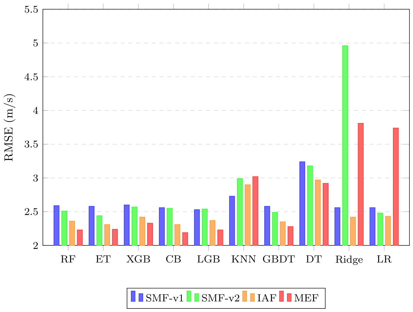
A notable anomaly is ridge regression, whose RMSE degrades sharply to 4.96 m/s—worse even than the uncorrected NWP baseline. This severe collapse indicates that the expanded feature set introduces multicollinearity and nonlinear feature interactions that the rigid linear model cannot accommodate. In contrast, linear regression maintains stable performance. This finding underscores the risk of applying regularized linear models to high-dimensional meteorological feature spaces without careful feature selection or dimensionality reduction.

5.1.3. Isobaric Atmospheric Features: IAFs

Table 4 presents the results with the IAF configuration, which incorporates upper-air variables at multiple pressure levels. The addition of three-dimensional atmospheric information yields further improvements across all the models, with RMSE decreasing by 0.44–1.10 m/s relative to the baseline. CatBoost emerges as the best model, closely followed by extra trees. The consistent improvement across all the methods confirms that vertical atmospheric structure, including wind shear, temperature stratification, and upper-level circulation patterns, provides valuable information for surface wind speed correction that is not captured by surface observations alone.

Table 4. Wind speed correction performance using the IAF feature set.

Method	RMSE (m/s)	MAE (m/s)
CMA-WSP 2.0 (Baseline)	3.41	2.50
Random Forest	2.36	1.63
Extra Trees	2.31	1.59
XGBoost	2.42	1.67
CatBoost	2.31	1.58
LightGBM	2.37	1.64
KNN	2.90	2.06
GBDT	2.35	1.64
Decision Tree	2.97	2.17
Ridge Regression	2.42	1.68
Linear Regression	2.43	1.69

Particularly noteworthy is the behavior of the weaker models. Decision tree improves substantially from an RMSE of 3.18 m/s to 2.97 m/s and KNN improves from 2.99 to 2.90 m/s, suggesting that the upper-air features provide more discriminative information that even simple models can leverage. Ridge regression also recovers from its SMF-v2 collapse, returning to a reasonable RMSE of 2.42 m/s.

5.1.4. Multi-Model Ensemble Features: MEFs

Table 5 reports the results with the full MEF configuration, which integrates forecasts from both CMA-WSP 2.0 and ECMWF. The tree-based ensemble and gradient boosting methods achieve their best performance under this configuration, with RMSE decreasing by 0.49–1.22 m/s relative to the baseline. CatBoost achieves the lowest overall error, with random forest and LightGBM tied for second.

Table 5. Wind speed correction performance using the MEF feature set.

Method	RMSE (m/s)	MAE (m/s)
CMA-WSP 2.0 (Baseline)	3.41	2.50
Random Forest	2.23	1.50
Extra Trees	2.24	1.54
XGBoost	2.33	1.62
CatBoost	2.19	1.50
LightGBM	2.23	1.51
KNN	3.02	2.22
GBDT	2.28	1.55
Decision Tree	2.92	2.12
Ridge Regression	3.81	2.15
Linear Regression	3.74	2.12

The multi-model features, however, do not benefit all the methods uniformly. KNN, ridge regression, and linear regression all degrade relative to the IAF configuration. This divergence reveals a critical insight. When the feature space becomes high-dimensional through multi-model concatenation, methods that rely on distance metrics in the full feature space or assume a global linear relationship suffer from the curse of dimensionality, whereas tree-based methods are inherently more robust to high-dimensional inputs.

5.1.5. Summary of Wind Speed Correction Results

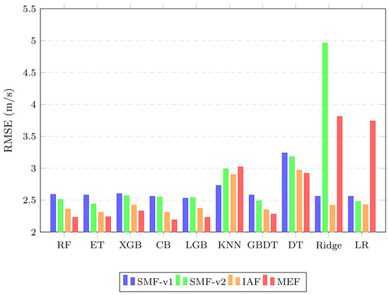
Table 6 summarizes the best achievable result at each feature engineering level, and Figure 4 provides a visual comparison of all the methods across the four configurations. The progressive enrichment of features yields consistent gains. The best RMSE decreases monotonically from 2.53 m/s to 2.19 m/s, a cumulative improvement of 0.34 m/s from feature engineering alone. The best overall configuration, CatBoost with the MEF feature set, reduces the RMSE by 1.22 m/s and the MAE by 1.00 m/s relative to the uncorrected CMA-WSP 2.0 forecast.

Table 6. Best-performing model at each feature engineering level for 70 m wind speed correction.

Features	Best Model	RMSE (m/s)	MAE (m/s)
Baseline (CMA-WSP 2.0)	—	3.41	2.50
SMF-v1	LightGBM	2.53	1.80
SMF-v2	Extra Trees	2.44	1.70
IAFs	CatBoost	2.31	1.58
MEFs	CatBoost	2.19	1.50

Figure 4. Wind speed correction RMSE for all ten methods across the four feature configurations.

Several important patterns emerge from these results. First, the six tree-based methods consistently form the top-performing group across all the feature configurations. This suggests that the marginal differences among boosting implementations are small relative to the gains that are achievable through feature engineering. This indicates that, within the recommended model class, feature engineering contributes more to accuracy than the choice among competitive tree-based learners. This observation does not extend to the clearly underperforming single-tree and distance-based methods, whose errors remain large regardless of feature enrichment. Second, model robustness to feature dimensionality is highly asymmetric. KNN degrades monotonically as features are added, and ridge regression collapses catastrophically under SMF-v2 and MEFs, whereas tree-based methods remain robust or continue to improve.

5.2. Results of Wind Power Forecasting

5.2.1. Xinjiang Wind Farm

Table 7 presents the overall performance on the Xinjiang wind farm dataset. Among the traditional ML models, extra trees achieves the best performance, while GBDT ranks last. Within the time-series family, DLinear outperforms recurrent architectures such as LSTM and GRU. TSMixer and TCN also demonstrate strong performance, suggesting that models specifically designed for time series are well suited to wind power forecasting. Among the Transformer-based models, Transformer–BiLSTM achieves the highest accuracy and qualification rate, followed closely by Informer and Autoformer. The hybrid architecture of Transformer–BiLSTM, which combines bidirectional LSTM temporal encoding with Transformer self-attention, appears to effectively capture both local temporal dynamics and long-range dependencies in the Xinjiang wind regime.

Table 7. Wind power forecasting performance on the Xinjiang wind farm dataset.

Family	Model	Accuracy (%)	Qualification Rate (%)
Traditional ML	Extra Trees	66.52	53.31
	SVR	65.88	52.70
	Random Forest	65.98	52.80
	Ridge	64.14	51.06
	LightGBM	64.80	51.68
	XGBoost	64.22	51.13
	GBDT	63.02	50.00
Time-Series DL	DLinear	83.72	69.55
	LightTS	80.48	66.49
	TimeMixer	81.28	67.24
	TSMixer	82.18	68.09
	LSTM	79.82	65.86
	GRU	80.70	66.69
	TCN	81.38	67.34
Transformer-based	Autoformer	82.64	68.53
	Crossformer	82.20	68.11
	FEDFormer	80.34	66.36
	Informer	82.74	68.62
	iTransformer	81.74	67.68
	Transformer–BiLSTM	84.20	70.00

5.2.2. Fujian Wind Farm

Table 8 presents the results on the Fujian wind farm dataset. Several important differences from the Xinjiang results emerge.

Table 8. Wind power forecasting performance on the Fujian wind farm dataset.

Family	Model	Accuracy (%)	Qualification Rate (%)
Traditional ML	Extra Trees	66.04	54.34
	SVR	62.92	51.07
	Random Forest	61.90	50.00
	Ridge	68.76	57.20
	LightGBM	73.56	62.24
	XGBoost	67.12	55.48
	GBDT	69.58	58.06
Time-Series DL	DLinear	78.22	67.12
	LightTS	78.82	67.75
	TimeMixer	79.24	68.20
	TSMixer	74.08	62.78
	LSTM	71.48	60.05
	GRU	73.52	62.19
	TCN	77.68	66.56
Transformer-based	Autoformer	80.96	70.00
	Crossformer	78.52	67.44
	FEDFormer	77.96	66.85
	Informer	78.24	67.15
	iTransformer	80.64	69.66
	Transformer–BiLSTM	78.96	67.90

First, the overall accuracy levels are lower across all the model families. The best-performing model on this dataset is Autoformer rather than Transformer–BiLSTM. This dataset-dependent performance variation suggests that no single architecture dominates universally. Rather, the relative suitability of a model depends on the characteristics of the wind regime.

Second, the performance gap between model families narrows. The best traditional ML model narrows the gap with the deep learning models. The recurrent architectures are disproportionately affected. By contrast, iTransformer, Autoformer, and TimeMixer decline more slowly. This pattern indicates that models relying on sequential state propagation are more sensitive to regime shifts than attention-based or multi-scale mixing architectures.

5.2.3. Cross-Dataset Comparison and Key Insights

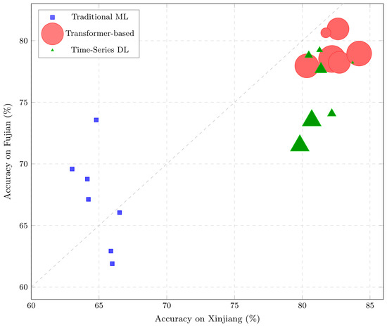
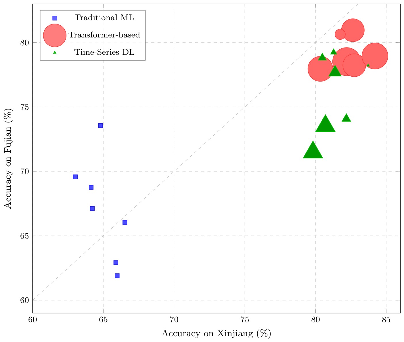
The comparative analysis across the two datasets, visualized in Figure 5, yields three key insights for wind power forecasting:

Figure 5. Cross-dataset stability analysis: accuracy on the Xinjiang dataset (x-axis) versus accuracy on the Fujian dataset (y-axis) for each model. The marker size of each point is proportional to the model’s weight memory. Points near the dashed diagonal line exhibit stable performance across wind regimes. Points below the line perform better on Xinjiang, while points above it perform better on Fujian.

• Deep learning models consistently and substantially outperform traditional ML. On both Xinjiang and Fujian, the average accuracy of the time-series and Transformer-based families exceeds that of traditional ML by a wide margin. This confirms that, for the temporal and nonlinear dynamics of wind power generation, deep learning architectures provide genuine modeling advantages that cannot be replicated by tree-based or linear methods alone.
• The model rankings are dataset-dependent, underscoring the value of multi-site evaluation. Transformer–BiLSTM ranks first on Xinjiang but falls to third among the Transformer-based models on Fujian. Conversely, Autoformer rises from third to first within the Transformer-based family, and iTransformer improves from fifth to second while exhibiting the smallest cross-dataset accuracy decline among all the deep learning models. A single-dataset study would therefore have produced misleadingly definitive rankings, validating our choice to evaluate models on geographically distant sites.
• Recurrent architectures are among the most sensitive to wind regime shifts. LSTM, GRU, and TSMixer exhibit the largest cross-dataset accuracy declines, whereas attention-based iTransformer and Autoformer are the most stable. Notably, Transformer–BiLSTM is markedly less stable across regimes than purely attention-based Autoformer and iTransformer, a pattern that is consistent with the hypothesis that its bidirectional recurrent branch retains the regime sensitivity of recurrent models.

In summary, deep learning models outperform the best traditional machine learning methods by a wide margin on both datasets, and this cross-farm gap is consistent across two geographically and climatologically distinct wind regimes.

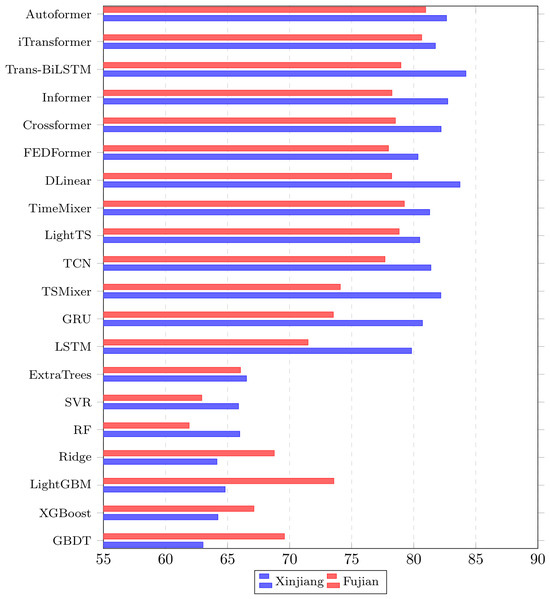
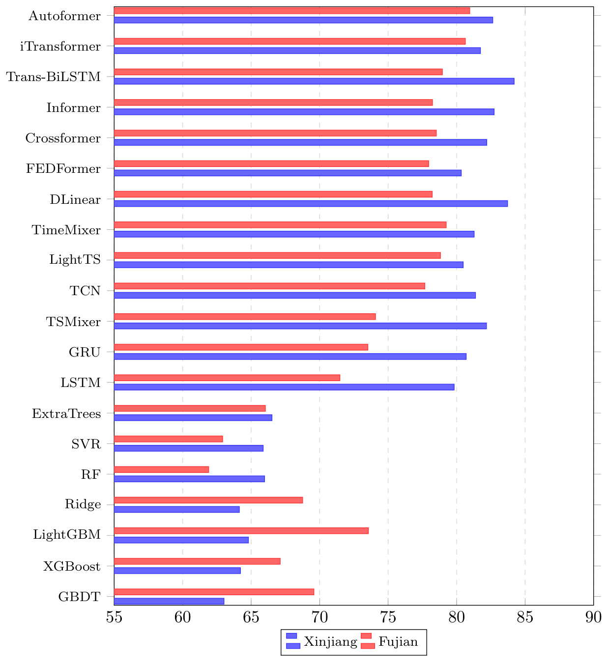
Figure 6 provides a visual comparison across all the models and both datasets. The results reveal a clear hierarchical pattern. The Transformer-based models achieve the highest accuracy, followed by the time-series deep learning models, with the traditional ML models lagging substantially.

Figure 6. Wind power forecasting accuracy for all 20 models on both datasets.

5.3. Discussion

5.3.1. RQ1: Machine Learning Methods for Wind Speed Correction

• Tree-based ensemble and gradient boosting methods consistently dominate. Across all four feature configurations, the six tree-based methods occupy the top six positions. This result is consistent with the findings of Sun et al. [16], who reported that RF and SVR outperformed deep learning for wind speed post-processing.
• Feature engineering matters more than model selection within the competitive model class. The gain that is attributable to feature enrichment exceeds the spread among the leading methods at any fixed feature level. This reinforces the argument of Zeng et al. [17] that enriching input features, particularly with spatial information from neighboring sources, is a more effective strategy for improving correction accuracy than pursuing increasingly complex model architectures.
• Model robustness varies dramatically with feature dimensionality. Under the basic SMF-v1 configuration, even simple models perform competitively. As feature dimensionality increases, however, some methods degrade monotonically. Tree-based methods, in contrast, are inherently robust to high-dimensional inputs owing to their implicit feature selection through recursive partitioning.

5.3.2. RQ2: Deep Learning for Wind Power Forecasting

• Deep learning models deliver substantial and consistent improvements over traditional ML. Across both datasets, the deep learning models achieve accuracy that far exceeds that of the traditional ML methods. On Xinjiang the improvement is particularly pronounced, while on Fujian the gap narrows but remains significant. This confirms that wind power forecasting, a task that is characterized by complex temporal dependencies and nonlinear power curve dynamics, benefits genuinely from deep learning architectures.
• No single architecture dominates across all the wind regimes. Transformer–BiLSTM ranks first on Xinjiang but only third among the Transformer-based models on Fujian, whereas Autoformer moves from third to first and iTransformer from fifth to second. This pattern is consistent with the hypothesis that attention-based representations, which compute temporal dependencies globally within each input window rather than through sequential state propagation, are less disrupted by the distributional shift between inland and coastal regimes.
• Recurrent architectures are the most sensitive to dataset characteristics. LSTM and GRU experience the largest cross-dataset performance declines among the recurrent models, falling behind not only other deep learning models but also the best traditional ML model. This vulnerability likely stems from the recurrent architecture’s reliance on sequential state propagation, which is more susceptible to disruption by the higher volatility and non-stationarity of the coastal wind regime.

5.3.3. Synthesis: Does Machine Learning Improve Wind Power Forecasting?

• For wind speed correction: The tree-based ensemble and gradient boosting methods consistently outperform or match all the other model families across the four feature configurations. Moreover, the performance gains from enriching meteorological features substantially exceed the gains from switching between model architectures within any fixed feature set. In this regime, the added complexity of deep learning is unwarranted.
• For wind power forecasting: Deep learning models consistently and substantially outperform traditional ML. However, no single architecture dominates universally. Among the deep learning architectures, attention-based models exhibit the greatest cross-regime robustness, while recurrent architectures are the most sensitive to regime shifts.
• Overall: The two stages of the wind power forecasting pipeline exhibit fundamentally different characteristics. Wind speed correction operates on structured tabular data with physically meaningful features, where tree-based methods excel and complexity yields diminishing returns. Wind power forecasting involves temporal dependencies and nonlinear power curve dynamics that favor deep learning approaches, with attention-based architectures offering the best trade-off between accuracy and cross-regime robustness.

6. Conclusions

In this paper, we conducted a systematic experimental investigation to evaluate whether machine learning improves wind power forecasting. We decomposed this question into two sub-tasks, i.e., wind speed correction and wind power forecasting, and evaluated a comprehensive set of methods on real-world datasets under consistent experimental protocols. Our study provides robust evidence that the question of whether machine learning improves wind power forecasting does not admit a simple yes-or-no answer. The answer depends on the specific task, the characteristics of the data, and the performance criteria of interest. We hope that these findings encourage more nuanced task-specific benchmarking in the wind power forecasting community and help practitioners to make informed decisions about model selection.

References

- Liu, Y.; Wang, Y.; Wang, Q.; Zhang, K.; Qiang, W.; Wen, Q.H. Recent advances in data-driven prediction for wind power. Front. Energy Res. 2023, 11, 1204343. [Google Scholar] [CrossRef] [Scilit]
- Zhao, X.; Sun, Q.; Tang, W.; Yu, S.; Wang, B. A comprehensive wind speed forecast correction strategy with an artificial intelligence algorithm. Front. Environ. Sci. 2022, 10, 1034536. [Google Scholar] [CrossRef] [Scilit]
- Yang, M.; Guo, Y.; Wang, B.; Wang, Z.; Chai, R. A day-ahead wind speed correction method: Enhancing wind speed forecasting accuracy using a strategy combining dynamic feature weighting with multi-source information and dynamic matching with improved similarity function. Expert Syst. Appl. 2025, 263, 125724. [Google Scholar] [CrossRef] [Scilit]
- Li, M.; Yang, M.; Yu, Y.; Lee, W.J. A Wind Speed Correction Method Based on Modified Hidden Markov Model for Enhancing Wind Power Forecast. IEEE Trans. Ind. Appl. 2022, 58, 656–666. [Google Scholar] [CrossRef] [Scilit]
- Liu, X.; Li, Z.; Shen, Y. Study on Downscaling Correction of Near-Surface Wind Speed Grid Forecasts in Complex Terrain. Atmosphere 2024, 15, 1090. [Google Scholar] [CrossRef] [Scilit]
- Xu, Y.; Yuan, H.S.; Sun, Z.D.; Chang, Y.; Shen, C. EOF-Based Bias Correction of Near-Surface Wind Speed Over China Reveals Stronger Future Trends and Variability. Geophys. Res. Lett. 2026, 53, e2025GL120559. [Google Scholar] [CrossRef] [Scilit]
- Guo, Z.; Lyu, Z.; Liu, Y. Challenge and Bias Correction for Surface Wind Speed Prediction: A Case Study in Shanxi Province, China. Climate 2025, 13, 150. [Google Scholar] [CrossRef] [Scilit]
- Hanifi, S.; Liu, X.; Lin, Z.; Lotfian, S. A Critical Review of Wind Power Forecasting Methods—Past, Present and Future. Energies 2020, 13, 3764. [Google Scholar] [CrossRef] [Scilit]
- Yan, J.; Li, Y.; Wang, H.; Han, S.; Shang, W.; Liu, Y. Wind Power Forecasting Based on Large Time Series Model. Engineering 2025. [Google Scholar] [CrossRef] [Scilit]
- Guo, X.; Zeng, P.; Xiong, X.; Wang, G.; Cui, Y. Short-term wind power forecasting methods based on machine learning: A review and case study. Energy Rep. 2025, 14, 3753–3782. [Google Scholar] [CrossRef] [Scilit]
- Wang, Y.; Zou, R.; Liu, F.; Zhang, L.; Liu, Q. A review of wind speed and wind power forecasting with deep neural networks. Appl. Energy 2021, 304, 117766. [Google Scholar] [CrossRef] [Scilit]
- Wang, D.; Xu, M.; Guangming, Z.; Luo, F.; Gao, J.; Chen, Y. Enhancing wind power forecasting accuracy through LSTM with adaptive wind speed calibration (C-LSTM). Sci. Rep. 2025, 15, 5352. [Google Scholar] [CrossRef] [Scilit] [PubMed]
- Wang, S.; Liu, H.; Yu, G. Short-term wind power combination forecasting method based on wind speed correction of numerical weather prediction. Front. Energy Res. 2024, 12, 1391692. [Google Scholar] [CrossRef] [Scilit]
- Yang, S.; Tang, J.; Ye, L.; Liu, J.; Zhao, W. An Improved Wind Power Forecasting Model Considering Peak Fluctuations. Electronics 2025, 14, 3050. [Google Scholar] [CrossRef] [Scilit]
- Zhang, Y. TSG-Net: A Multiscale Decomposition and Spatio-Temporal Graph Neural Network Framework for High-Precision Wind Power Forecasting. Wind Energy 2026, 29, e70100. [Google Scholar] [CrossRef] [Scilit]
- Sun, L.; Lan, Y.; Sun, X.; Liang, X.; Wang, J.; Su, Y.; He, Y.; Xia, D. Deterministic forecasting and probabilistic post-processing of short-term wind speed using statistical methods. J. Geophys. Res. Atmos. 2024, 129, e2023JD040134. [Google Scholar] [CrossRef] [Scilit]
- Zeng, Z.; Wu, H.; Liu, Z.; Zhao, L.; Liang, Z.; Liang, Z.; Wang, Y. Enhancing short-term wind speed prediction capability of numerical weather prediction through machine learning methods. J. Geophys. Res. Atmos. 2024, 129, e2024JD041822. [Google Scholar] [CrossRef] [Scilit]
- Jonas, S.; Winter, K.; Brodbeck, B.; Meyer, A. Bias correction of wind power forecasts with SCADA data and continuous learning. J. Phys. Conf. Ser. 2024, 2767, 092061. [Google Scholar] [CrossRef] [Scilit]
- Aye, H.Y.; Scala, F.; Štěpanec, L.; Lin, O.Z.; Juchelkova, D. Mechanistic machine learning for biomass pyrolysis: Integrating lignocellulosic structure, thermal severity, and multi-objective optimization for organic bio-oil yield. Energy Convers. Manag. X 2026, 31, 102137. [Google Scholar] [CrossRef] [Scilit]
- Lin, O.Z.; Štěpanec, L.; Koutroulis, E.; Juchelkova, D.; Aye, H.Y. Optimizing monthly solar PV tilt angles and energy yield across global climate zones: A hybrid machine learning and PVLib approach. Renew. Energy 2026, 260, 125163. [Google Scholar] [CrossRef] [Scilit]
- Glahn, H.R.; Lowry, D.A. The use of model output statistics (MOS) in objective weather forecasting. J. Appl. Meteorol. Climatol. 1972, 11, 1203–1211. [Google Scholar] [CrossRef] [Scilit] [PubMed]
- Sun, Q.; Jiao, R.; Xia, J.; Yan, Z.; Li, H.; Sun, J.; Wang, L.; Liang, Z. Adjusting wind speed prediction of numerical weather forecast model based on machine learning methods. Meteorol. Mon. 2019, 45, 426–436. (In Chinese) [Google Scholar] [CrossRef]
- Fang, Y.; Wu, Y.; Wu, F.; Yan, Y.; Liu, Q.; Liu, N.; Xia, J. Short-term wind speed forecasting bias correction in the Hangzhou area of China based on a machine learning model. Atmos. Ocean. Sci. Lett. 2023, 16, 100339. (In Chinese) [Google Scholar] [CrossRef] [Scilit]
- Ren, P.; Chen, M.; Cao, W.; Wang, Z.; Han, L.; Song, L.; Yang, L. Error analysis and correction of short-term numerical weather prediction under complex terrain based on machine learning. Acta Meteorol. Sin. 2020, 78, 1002–1020. (In Chinese) [Google Scholar] [CrossRef]
- He, H.; He, W.; Guo, J.; Wu, K.; Zhao, W.; Wan, Z. Research on New Energy Power Generation Forecasting Method Based on Bi-LSTM and Transformer. Energies 2025, 18, 5165. [Google Scholar] [CrossRef] [Scilit]
- Vaswani, A.; Shazeer, N.; Parmar, N.; Uszkoreit, J.; Jones, L.; Gomez, A.N.; Kaiser, Ł.; Polosukhin, I. Attention is all you need. In Advances in Neural Information Processing Systems; Curran Associates, Inc.: Red Hook, NY, USA, 2017; Volume 30. [Google Scholar] [CrossRef] [Scilit]
- Wang, H.K.; Li, D.; Chen, F.; Du, J.; Song, K. GCNInformer: A combined deep learning model based on GCN and Informer for wind power forecasting. Energy Sci. Eng. 2023, 11, 3836–3854. [Google Scholar] [CrossRef] [Scilit]
- Zhu, M.; Li, Z.; Lin, Q.; Ding, L. Fast-powerformer: A memory-efficient transformer for accurate mid-term wind power forecasting. arXiv 2025, arXiv:2504.10923. [Google Scholar] [CrossRef] [Scilit]
- Elmousalami, H.; Elmesalami, H.H.; Maxi, M.; Farid, A.A.K.M.; Elshaboury, N. A comprehensive evaluation of machine learning and deep learning algorithms for wind speed and power prediction. Decis. Anal. J. 2024, 13, 100527. [Google Scholar] [CrossRef] [Scilit]
Disclaimer/Publisher’s Note: The statements, opinions and data contained in all publications are solely those of the individual author(s) and contributor(s) and not of MDPI and/or the editor(s). MDPI and/or the editor(s) disclaim responsibility for any injury to people or property resulting from any ideas, methods, instructions or products referred to in the content. |
© 2026 by the authors. Licensee MDPI, Basel, Switzerland. This article is an open access article distributed under the terms and conditions of the Creative Commons Attribution (CC BY) license.