


Highlights
What are the main findings?
- The GRU architecture provides superior robustness and forecasting capability under highly volatile and nonstationary conditions, as supported by both error metrics and Diebold–Mariano statistical tests.
- Forecasting performance depends strongly on the temporal characteristics and variability of local dynamics rather than on model complexity alone, with no single architecture consistently dominating across all provinces.
What are the implications of the main findings?
- The findings suggest that recurrent architecture selection should be guided by the temporal volatility regime of the target environment rather than architectural complexity alone, providing practical guidance for forecasting model deployment in severely polluted regions of Southeast Asia.
- The systematic behavioural differences identified across recurrent architectures under heterogeneous volatility regimes establish a reproducible methodological baseline for future development of advanced hybrid, ensemble, or probabilistic forecasting frameworks for in northern Thailand.
Abstract
Forecasting concentrations remains a challenging data science problem because of strong nonlinearity, temporal dependence, and pronounced nonstationarity associated with seasonal and episodic pollution events. This study presents a comparative evaluation of recurrent neural network architectures for one-day-ahead forecasting using daily observations from four provinces in northern Thailand with varying pollution dynamics. Standard RNN, LSTM, and GRU models were developed within a unified forecasting framework using historical concentrations and meteorological variables as predictors. Model performance was evaluated on an independent test dataset using , , and , together with Diebold–Mariano tests based on forecast error series. The experimental results indicate that the GRU model provides more robust forecasting performance under conditions of strong volatility and nonstationary behaviour, while the LSTM and RNN models remain competitive in comparatively more stable environments. No single model consistently dominated across all provinces, indicating that forecasting effectiveness depends strongly on the temporal characteristics of local air pollution dynamics rather than on architectural complexity alone. While all models capture the overall seasonal structure of variation, extreme pollution peaks are systematically underestimated partly because MSE-based training biases predictions toward the central tendency of the data distribution. However, gated architectures show improved responsiveness to abrupt concentration changes relative to the standard RNN. These findings highlight the importance of matching recurrent architectural design to the temporal regime of the target environment.
1. Introduction
air pollution has become one of the most serious environmental and public health challenges worldwide. According to the World Health Organization (WHO), nearly 99% of the global population was exposed to unhealthy levels of fine particulate matter in 2019, contributing to approximately 7 million premature deaths annually [1]. Fine particulate matter with aerodynamic diameters smaller than 2.5 micrometres () has attracted increasing global attention because of its severe impacts on human health, environmental sustainability, and social welfare [2,3,4]. Exposure to elevated concentrations is strongly associated with respiratory and cardiovascular diseases, chronic respiratory disorders, and premature mortality [5,6]. Beyond health consequences, severe pollution also disrupts transportation, tourism, economic activity, and quality of life. In Thailand, the problem becomes particularly severe in the northern region during the dry season, when biomass burning and transboundary haze pollution generate extreme and rapidly changing episodes [7]. Satellite-derived observations from the Geo-Informatics and Space Technology Development Agency (GISTDA) reported that more than 10 million rai of land across 17 northern provinces were affected by burning activities between January and May 2024, with Mae Hong Son, Chiang Mai, Lampang, and Tak among the most severely affected areas [8]. These conditions create highly dynamic patterns characterised by strong temporal variability, abrupt fluctuations, and pronounced seasonal peaks. While short-term forecasting can support early-warning systems, pollution mitigation planning, and public health protection, time series often exhibit strong nonlinearity, temporal dependence, seasonal heterogeneity, and nonstationary behaviour, making accurate forecasting a difficult problem.
Previous studies have demonstrated strong relationships between concentrations and meteorological variables such as temperature, relative humidity, wind speed, wind direction, and precipitation [9,10,11]. These meteorological factors influence pollutant dispersion, accumulation, atmospheric transport, and chemical transformation processes [12,13]. Consequently, a wide range of statistical forecasting, numerical forecasting, machine learning (ML), and deep learning (DL) approaches have been developed for prediction. Statistical forecasting methods commonly rely on regression and time series analyses, while numerical forecasting methods employ physics-based atmospheric simulation models. With the rapid advancement of artificial intelligence, data-driven approaches, particularly ML and DL methods, have become increasingly important because of their ability to learn complex nonlinear relationships and temporal dependencies directly from data. Previous studies have applied ML approaches such as support vector machines (SVMs), random forests (RF), artificial neural networks (ANNs), k-nearest neighbours, extreme gradient boosting (XGBoost), generalised regression neural networks, and ensemble learning frameworks for prediction in different regions [9,11,14].
More recently, DL approaches have gained increasing attention for environmental time series forecasting. Recurrent neural network architectures, including recurrent neural networks (RNNs), long short-term memory (LSTM) networks [15,16], and gated recurrent unit (GRU) models [17], have been adopted because of their ability to capture temporal dependencies in sequential data [18]. Several studies have reported improved forecasting performance using gated recurrent architectures and hybrid DL frameworks that integrate convolutional neural networks, decomposition methods, and attention mechanisms [3,19,20,21,22,23,24,25,26,27]. In Thailand, ML and DL approaches have increasingly been applied to air quality forecasting [28,29,30]. Previous studies explored LSTM, CNN–LSTM, ConvLSTM, and spatiotemporal ensemble frameworks for prediction in Bangkok, Southern Thailand, and the Bangkok metropolitan region [31,32,33,34,35]. These studies demonstrated the potential of DL approaches for forecasting, particularly for capturing nonlinear and spatiotemporal patterns in air pollution data.
Recent advances in forecasting have increasingly emphasised complex hybrid and ensemble deep learning architectures aimed at maximising predictive accuracy. In contrast, comparatively less attention has been given to understanding how recurrent neural network architectures behave under highly volatile and nonstationary conditions. Although advanced architectures are highly effective, recurrent models remain important because they are simpler, more interpretable, computationally efficient, suitable for limited environmental datasets, and provide a practical baseline for forecasting concentrations under nonstationary conditions.
This study uses daily concentrations and meteorological variables from Mae Hong Son, Chiang Mai, Lampang, and Tak provinces to develop a unified comparative forecasting framework based on standard RNN, LSTM, and GRU architectures. No previous study has comprehensively compared these three architectures for one-day-ahead forecasting across multiple northern provinces of Thailand under identical data and training conditions. The novelty of this study lies in providing a systematic comparative analysis of recurrent neural network behaviour under distinct temporal variability regimes using a unified framework. Rather than emphasising architectural complexity, this work focuses on isolating the effects of recurrent architectural design on forecasting robustness and responsiveness to abrupt pollution changes. By examining recurrent model behaviour across distinct temporal regimes, this study provides practical insights for short-term air quality forecasting and contributes to a broader understanding of recurrent neural network behaviour under nonlinear and nonstationary environmental conditions. Finally, notwithstanding the fact that is affected by transboundary pollution, regional transport, and biomass-burning emissions, wind direction was excluded from the meteorological predictor set because of data incompleteness and the additional complexity associated with circular variable encoding; this is acknowledged as a limitation of the current study.
2. Materials and Methods
In this section, the data collection process—including study locations, variables and data splitting—is explained, and the deep learning methods used, loss function, hyperparameter optimisation, overfitting prevention, and performance measures are described. Moreover, the workflow for developing the deep learning models is presented.
2.1. Data Collection
The four provinces studied in this research, Mae Hong Son, Chiang Mai, Lampang, and Tak, are considered to experience the highest heat levels in the northern region of Thailand, primarily due to extensive burning activities exceeding one million rai, as reported in the 2024 GISTDA report [8]. The data used in this study are secondary data obtained from observation stations operated by Thai government agencies. The environmental variable considered is the daily average concentration (24 h average, in µg/m3), collected from the websites of the Pollution Control Department, Air Quality and Noise Management Bureau, Ministry of Natural Resources and Environment of Thailand [36], and GISTDA [37]. The Pollution Control Department measures concentrations primarily using standard instruments and techniques, mainly through automatic monitoring systems. The main technologies employed include the beta-ray attenuation method, a widely used approach in major air quality monitoring stations (e.g., the MetOne BAM1020); the light scattering method, which utilises US-EPA-certified sensors (e.g., Teledyne T640); and the gravimetric method, the reference standard for particulate matter analysis, which is used to calibrate and validate automatic instruments to ensure high data accuracy. The GISTDA applies space-based technologies to measure and predict concentrations, primarily using satellite observations. These include data from the Himawari satellite, the MODIS (Moderate Resolution Imaging Spectroradiometer) instruments on Terra and Aqua satellites, the VIIRS (Visible Infrared Imaging Radiometer Suite), the GEMS (Geostationary Environment Monitoring Spectrometer) onboard the KOMPSAT-2B satellite, and the Sentinel-5P satellite. The measurement mechanism is based on the analysis of atmospheric light reflection and absorption, expressed as aerosol optical depth. These data are integrated with artificial intelligence techniques to estimate real-time concentrations, which are then disseminated through web platforms and mobile applications.
Meteorological variables were obtained from the website of the Meteorological Information Subdivision, Northern Meteorological Center, Thai Meteorological Department (TMD) [38], and the Thai Meteorological Department Automatic Weather System [39]. The annual total number of observations for each province is provided in Table 1. The variables used to forecast daily average concentrations include season, 24 h average temperature (°C), 24 h average relative humidity (%), maximum wind speed (km/h), 24 h average air pressure (hPa), and precipitation (mm). In particular, our models forecast concentration at day t using the observed concentration at day (informed by the PACF analysis in Section 3), together with observed meteorological variables at day .
Table 1.
Number of daily average observations and missing records by province and year, covering the period from 1 January 2022 to 31 March 2026.
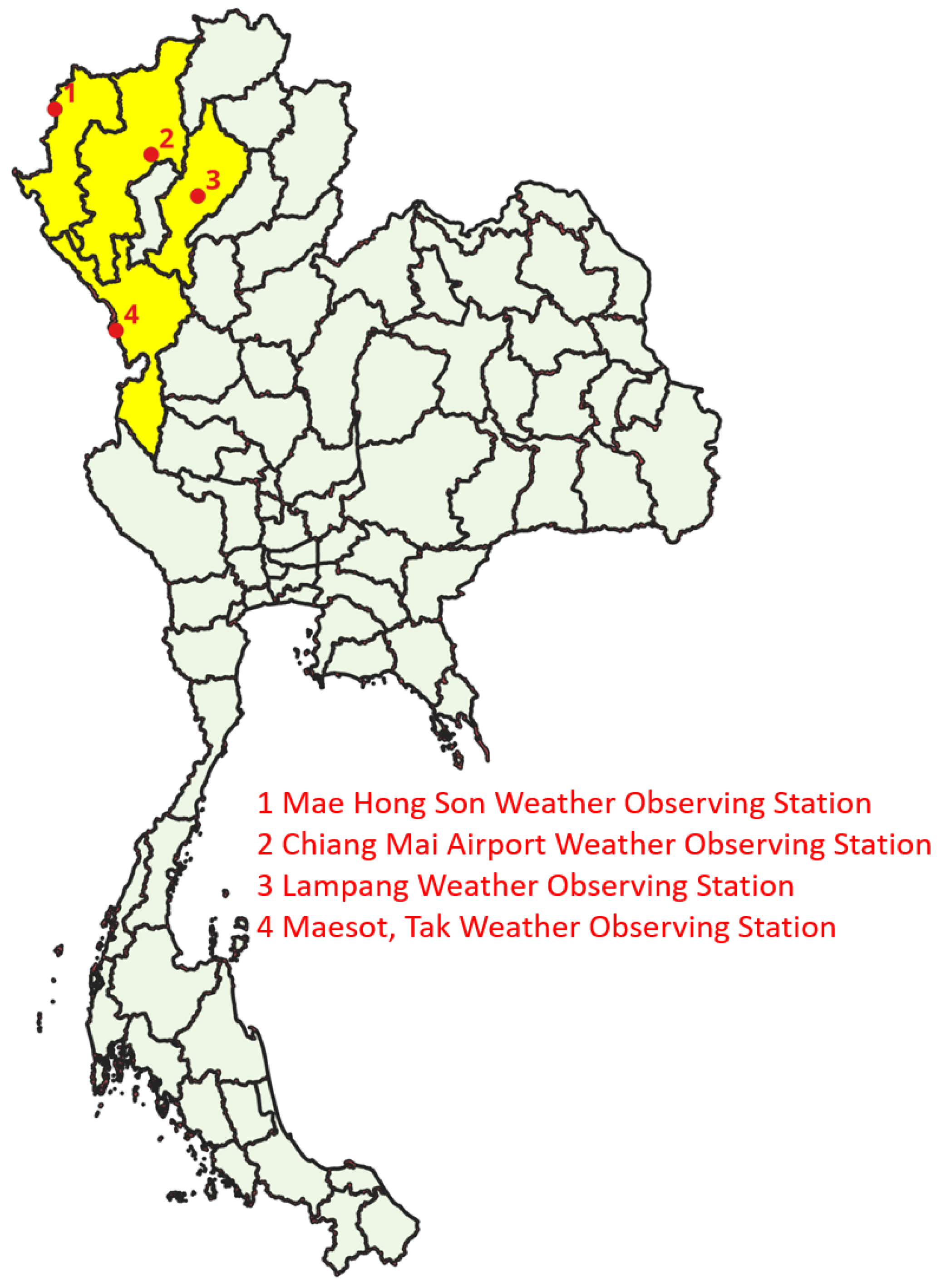
The locations of the four observing stations are as follows: Mae Hong Son Weather Observing Station (19.3° N, 97.97° E); Chiang Mai Airport Weather Observing Station (18.767° N, 98.967° E); Lampang Weather Observing Station (18.28° N, 99.52° E); and Mae Sot, Tak Weather Observing Station (16.67° N, 98.55° E). These are shown in the location map in Figure 1, which was created using QGIS software (version 4.0) [40] and a shapefile from the OCHA Services website [41]. Although all four provinces are located in the mountainous upper northern region of Thailand and are subject to the same seasonal biomass-burning cycle [8], they differ in physical setting in ways that are relevant to their dynamics. Mae Hong Son and Tak both lie along the Thailand–Myanmar border and are therefore directly exposed to transboundary smoke transported from agricultural and forest burning in neighbouring Myanmar and Shan State [7], in addition to local burning activity; their narrow, mountain-enclosed valley topography further restricts atmospheric dispersion, allowing pollutants to accumulate rather than disperse. Chiang Mai lies in a broader intermontane basin and combines local agricultural burning with urban and vehicular emissions, while Lampang, situated further from the international border, is comparatively more exposed to local and regional biomass burning than to direct transboundary transport. These differences in topography and source proximity are consistent with the province-level differences in variability reported in Table 2 and are revisited when interpreting model performance in Section 4.
Figure 1.
Map of Thailand showing locations of measurement stations in the northern region.
Table 2.
Descriptive statistics of daily average PM2.5 concentration (µg/m3) by province, 1 January 2022 to 31 March 2026.
2.2. Deep Learning Methods
This study compares three recurrent neural network architectures, the standard RNN [42,43], the LSTM [15,16,43], and the GRU [17], all of which process the input sequence by updating a hidden state at each time step using the current input and the previous hidden state. The LSTM extends the basic RNN with three gates (forget, input, output) and a separate cell state to mitigate the vanishing-gradient problem, while the GRU simplifies this design using only two gates (update, reset) and no separate cell state. Full mathematical definitions of the hidden-state update equations for all three architectures, together with the sum-of-squared-errors loss function used in training, are provided in Supplementary Material S1 for readers requiring the complete derivations.
Loss Function
For the RNN method with a quantitative output, training is achieved by minimising the sum-of-squares error loss function [42],
using a dataset consisting of n input–output sequence pairs , where is the input vector, is the observed output and is the last prediction in the sequence at time t. The parameters of both LSTM and GRU are estimated by minimising , where (see Supplementary Materials) represents the updated hidden state (or output vector) at time t.
2.3. Performance Measures
All models were trained using the R programming language. The results of different models were evaluated according to the coefficient of determination (), root mean squared error (), and mean absolute error (). Adapting the standard forms of these statistics, is defined as
where n is the number of input–output sequence pairs, denotes the observed output at time t, denotes the predicted output at time t of sequence length L, and denotes the average of observed output. Similarly, , given by
is the norm of the vector of differences between the observed and predicted output values, while , given by
is the norm.
In addition to , RMSE, and MAE, forecasting accuracy between pairs of competing models was compared using the Diebold–Mariano (DM) test [44]. This test evaluates the null hypothesis of equal predictive accuracy between two forecasts by testing whether the mean of the loss-differential series, i.e., the difference between the loss functions applied to each model’s forecast errors, is significantly different from zero. To assess whether conclusions about relative forecasting accuracy are sensitive to the choice of loss function, the DM statistics are computed under both a squared-error loss and an absolute-error loss. Additionally, because three pairwise model comparisons (RNN vs. LSTM, RNN vs. GRU, LSTM vs. GRU) were conducted within each of the four provinces, a Bonferroni-corrected significance threshold of was applied to control the family-wise error rate.
2.4. Study Workflow
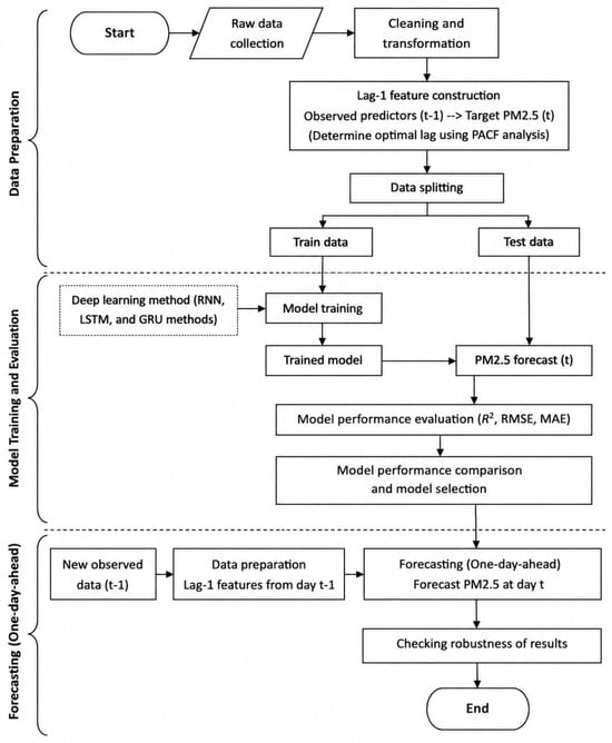
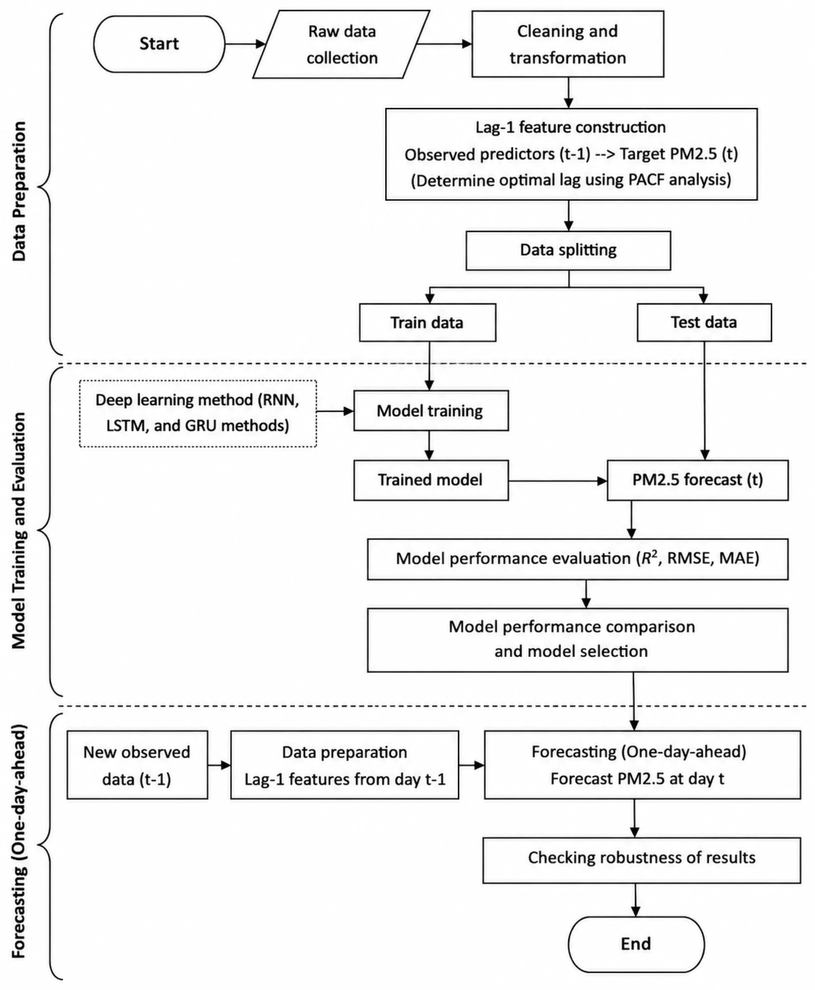
Comprehensive data preprocessing was applied to ensure quality and reliability, including systematic handling of missing values. Missing observations accounting for less than 5% of the dataset (see Table 1) were removed during preprocessing. Complete-case analysis was considered acceptable because the proportion of missing data was relatively small, consistent with the recommendation of Graham [45], who suggested that this approach may be appropriate when missing data are below approximately 5%. The dataset, divided into training (January 2022 to December 2024) and testing (January 2025 to March 2026) sets, as shown in Table 1, was organised into a supervised learning time series format suitable for deep neural networks. Because all predictor variables used for one-day-ahead forecasting were observed at day rather than forecast, the proposed framework did not rely on a separate meteorological forecasting model, and no error propagation from forecasted meteorological inputs was introduced into the forecasting process. Using the keras3 and tensorflow packages in the R programming language, multiple deep learning models were trained, with hyperparameters optimised through validation to improve forecasting robustness and evaluated on the test sets. Finally, a comparative analysis was conducted to benchmark and critically assess the predictive capability of the proposed models (see Figure 2).
Figure 2.
Process of the proposed forecasting framework.
3. Results
The descriptive statistics of daily average concentration for each province are summarised in Table 2. Mae Hong Son records the lowest mean concentration (25.25 µg/m3) and the largest standard deviation (39.49 µg/m3), together with the highest observed maximum (321.00 µg/m3), consistent with its exposure to intense and variable biomass-burning episodes. Lampang and Chiang Mai show higher variability (SD of 27.00 and 24.71 µg/m3, respectively), while Tak records the lowest variability (21.40 µg/m3).
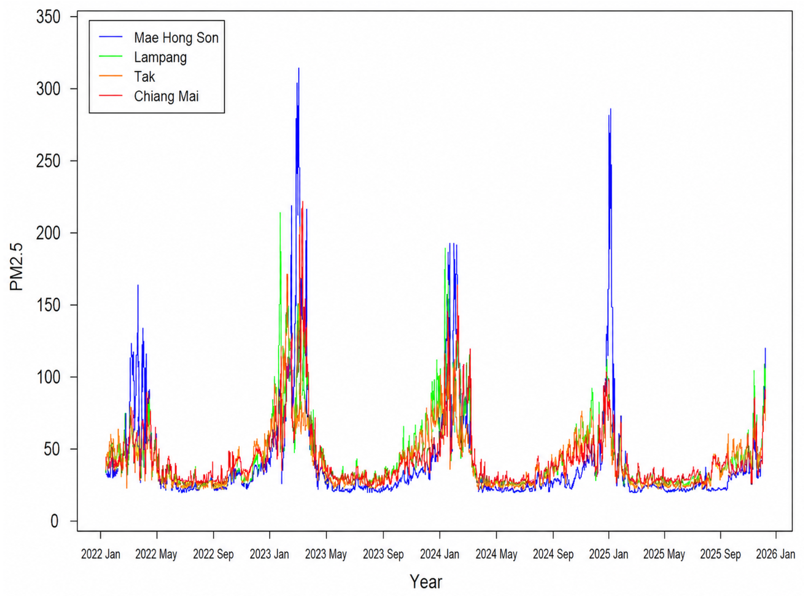
The trends in daily concentrations in Mae Hong Son, Lampang, Tak, and Chiang Mai provinces in upper northern Thailand from January 2022 to March 2026 are shown in Figure 3. concentrations across all provinces exhibit a clear seasonal pattern, characterised by pronounced peaks during the dry season (February–April) and substantial reductions during the rainy season (May–October). This pattern is consistent with regional biomass burning and meteorological conditions that limit atmospheric dispersion during dry periods, while precipitation and increased humidity during the wet season enhance pollutant removal. From a time series perspective, the data exhibit clear nonstationarity, with seasonal mean shifts and time-varying variance. During the dry season, levels exhibit substantially increased variance, indicating heteroscedasticity and heightened volatility. In contrast, concentrations during the rainy season are lower and more stable, reflecting a low-variance regime. This alternating high-variance and low-variance structure suggests regime-dependent dynamics that are important for forecasting model design.
Figure 3.
Annual concentration (µg/m3) trends across four provinces in northern Thailand from January 2022 to March 2026.
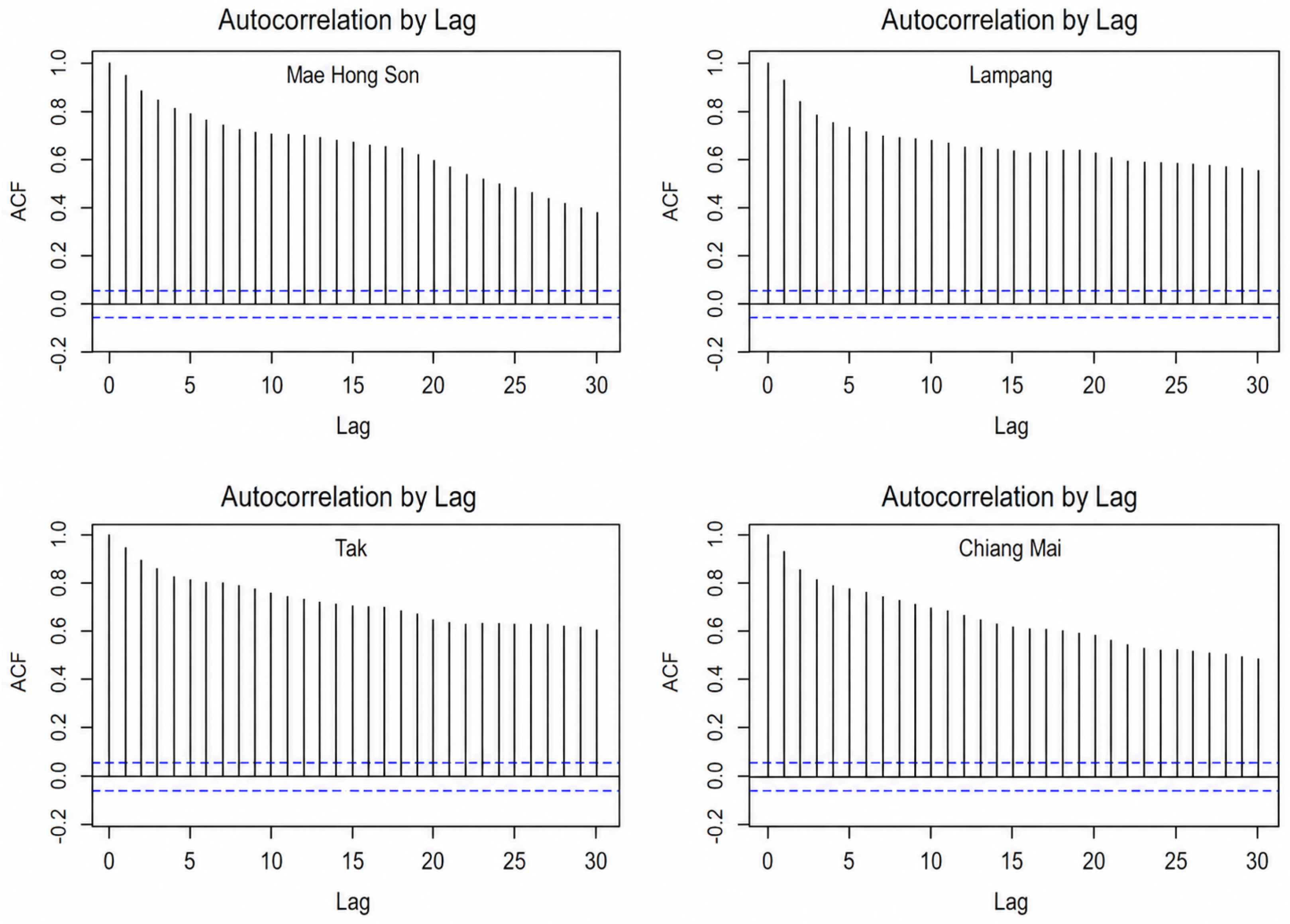
Before building the models, the autocorrelation function (ACF) and partial autocorrelation function (PACF) were used to examine the temporal characteristics of the data, reduce prediction errors, and improve forecasting accuracy. The ACF shows strong positive autocorrelation at short lags (1–5), with coefficients exceeding 0.6 and gradually decaying over time, indicating pronounced temporal dependence and persistent nonstationary behaviour in the series across all provinces. Current concentrations are therefore strongly influenced by recent observations, as shown in Figure 4.
Figure 4.
Autocorrelation function for of all four provinces by lag (days).
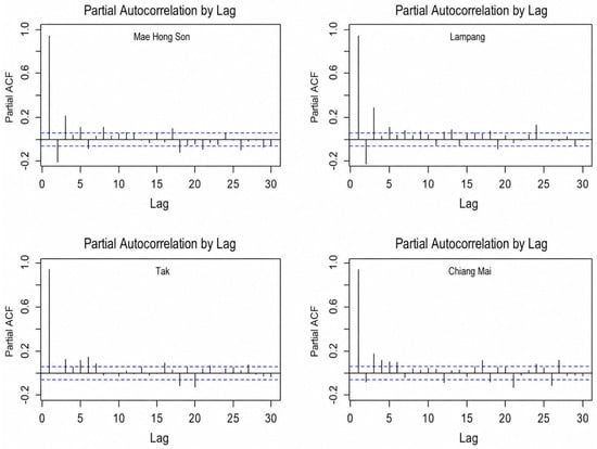
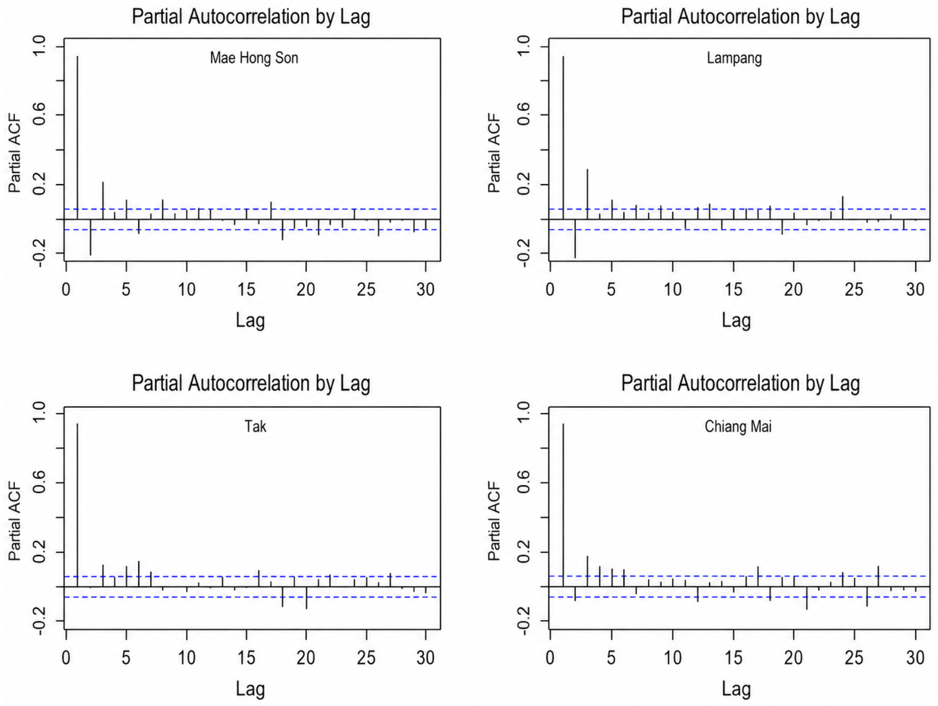
By contrast, the PACF exhibits a clear and dominant spike at lag-1, while most higher-order lags remain within the confidence bounds without a consistent pattern. This indicates that the primary temporal dependence is concentrated at the first lag, as shown in Figure 5. Therefore, a lag-1 input structure was selected for all forecasting models, as it effectively captures the main temporal dependency while maintaining model simplicity and reducing the risk of overfitting.
Figure 5.
Partial autocorrelation function for of all four provinces by lag (days).
3.1. Hyperparameter Optimisation and Overfitting Prevention
Hyperparameter settings for the deep learning models are summarised in Table 3, which lists the corresponding ranges used to identify the optimal model. The hyperparameters of the RNN, LSTM, and GRU models were optimised using a grid search approach based on validation performance, assessed using a cumulative (expanding-window) rolling cross-validation scheme. In other words, at each successive fold, the training window was expanded to include all observations up to a given time point, the model was fit on this expanding training set, and the immediately following six-month period was used to evaluate validation loss, after which the window boundary was rolled forward in time, and the training set expanded further. This procedure preserves the temporal ordering of the PM2.5 series and avoids the data leakage that would arise from randomly shuffled validation splits, while still providing multiple validation estimates. To produce more stable estimates, the cross-validation process was repeated 100 times. Variations in the number of hidden units, batch size, and number of epochs resulted in a total of 48 possible hyperparameter combinations. The optimal hyperparameter configuration was identified by selecting the configuration that achieved the lowest average validation loss across all folds and repetitions. This hyperparameter selection strategy aimed to balance model complexity, training stability, and generalisation performance.
Table 3.
Hyperparameters and ranges.
The learning rate was fixed at 0.001, a commonly adopted value that provides stable convergence when combined with the Root Mean Square Propagation (RMSprop) optimiser. To mitigate overfitting, a dropout rate of 0.5 was applied to randomly deactivate a subset of neurons during training. The sigmoid activation function was employed in the hidden layers to introduce nonlinearity, which is suitable for recurrent neural network models. Mean squared error () was selected as the loss function, as it is widely used for regression problems and effectively measures the discrepancy between predicted and observed values. A deterministic seed configuration was applied across R (version 4.6.0), Python (version 3.9), and TensorFlow (version 2.16.0) to ensure reproducibility, training stability, and consistency throughout the process. The final model configurations were selected to balance predictive performance and computational efficiency.
3.2. Performance Evaluation
This section evaluates the performance of the trained models on the test dataset and compares their relative suitability for one-day-ahead forecasting across the four northern provinces. Model performance was quantitatively assessed using standard regression metrics defined in Equations (1)–(3). Based on the results presented in Table 4, the predictive performance of the RNN, LSTM, and GRU models for one-day-ahead concentration forecasting exhibits variation across provinces. Table 5 reports the Diebold–Mariano (DM) test statistics, which are used to compare the forecasting accuracy of competing models.
Table 4.
Comprehensive evaluation of RNN, LSTM and GRU model performance on the test dataset.
Table 5.
The DM test statistics and p-values for comparing the forecasting accuracy between competing models.
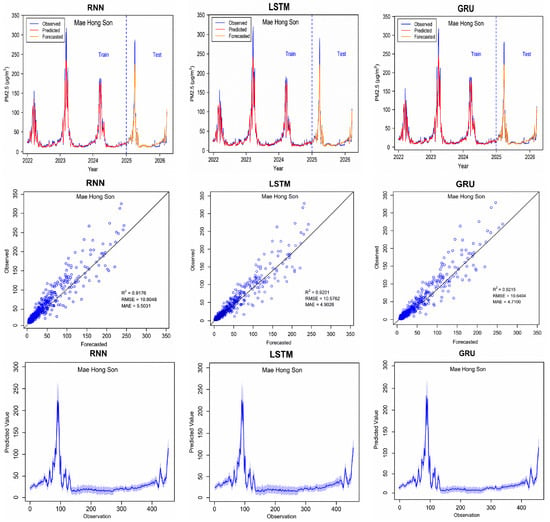
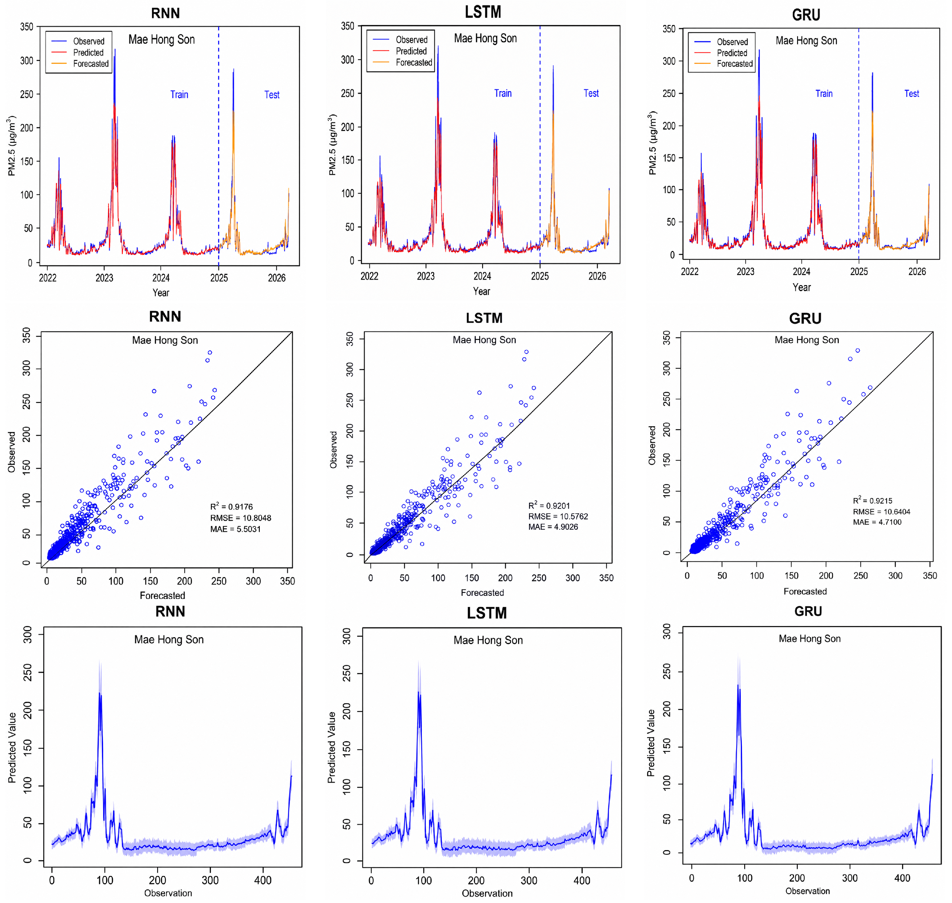
In Mae Hong Son, both the GRU and LSTM models demonstrate more robust forecasting performance under extreme pollution variability, achieving higher and lower and than the RNN model. This finding was statistically supported by the Diebold–Mariano tests after Bonferroni correction (), which indicated significant differences in accuracy based on the forecast error series using the absolute-error loss function. There is no evidence for a difference between the LSTM and GRU models using either squared-error or absolute-error loss functions. Figure 6 illustrates the temporal dynamics and model performance for this province, which exhibits the greatest variability and the most extreme episodes amongst the four provinces considered here. These extremes are particularly pronounced during the dry season, with sharp spikes reflecting the influence of intense biomass burning and transboundary pollution. The regression curve of observed and forecasted values for one-day-ahead forecasting exhibits moderate forecasting uncertainty under highly variable and extreme pollution conditions. The confidence interval bands in Mae Hong Son are generally wider than those observed in the other provinces, reflecting substantial predictive variability under these extreme conditions. Nevertheless, the GRU model produces noticeably narrower bands than the RNN and LSTM models, indicating greater stability and robustness during abrupt concentration changes.
Figure 6.
Performance of the RNN, LSTM, and GRU models for one-day-ahead forecasting in Mae Hong Son. The top-row panels show the observed and predicted (µg/m3) time series; the middle-row panels show observed versus forecasted (µg/m3) values; and the bottom-row panels show the confidence interval bands of the predicted values based on 500 replications.
Although all models capture the overall seasonal pattern, extreme peaks are frequently underestimated, particularly by the standard RNN. Two factors contribute to this: first, high-pollution observations are scarce relative to the full training dataset (data imbalance); second, the MSE loss function penalises large deviations quadratically and therefore biases predictions toward the central tendency of the data distribution, systematically smoothing out peak values.
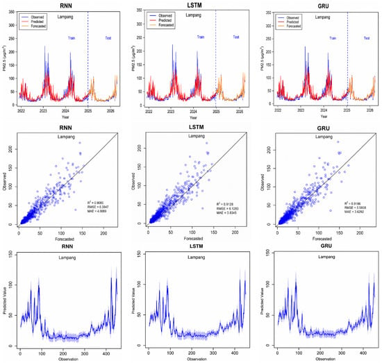
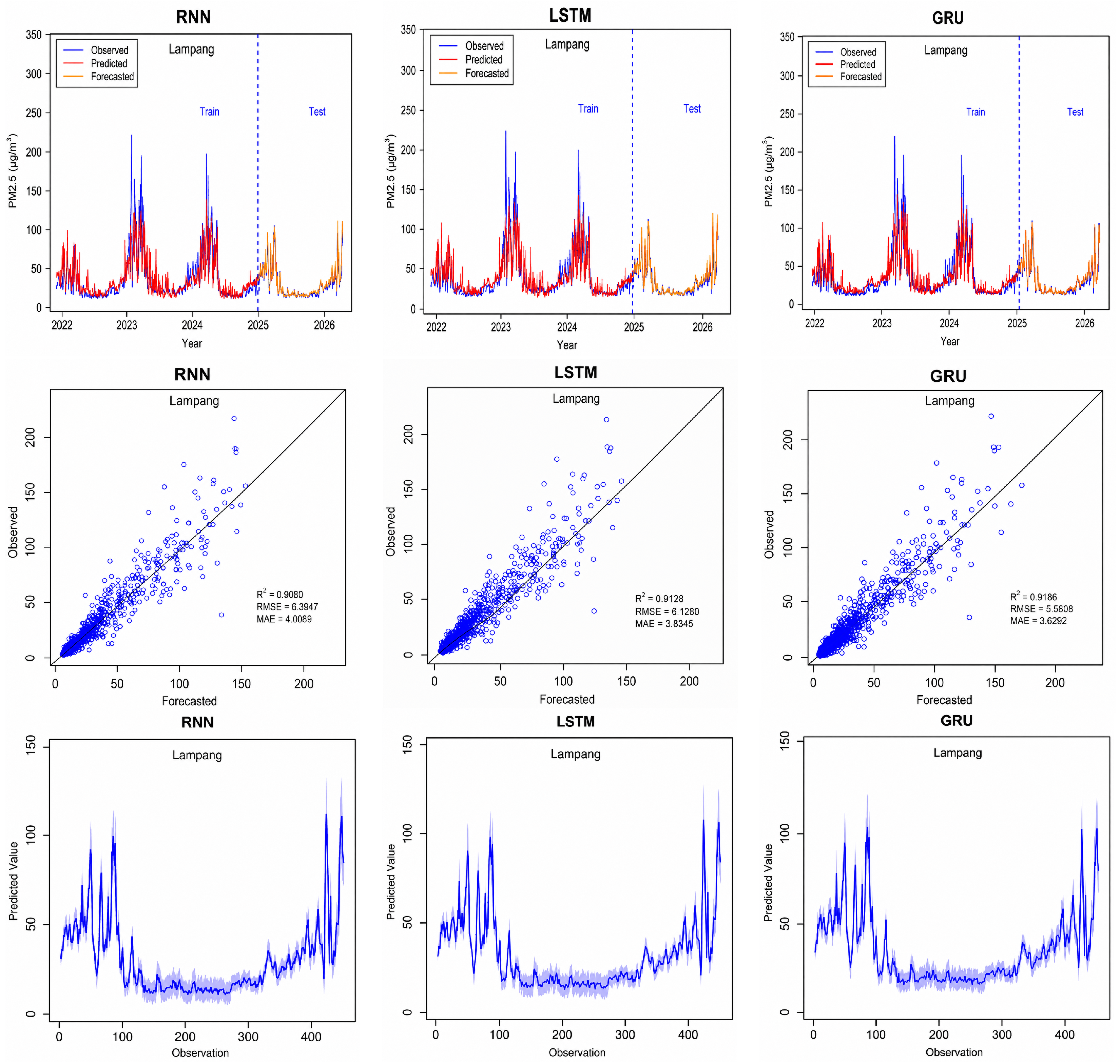
Lampang, along with Mae Hong Son, exhibits the highest overall predictive accuracy among the evaluated provinces. The GRU model slightly outperforms the others in terms of all three measures. The Diebold–Mariano test indicated significant differences in accuracy using squared-error and absolute-error loss functions, except for the comparison between the LSTM and GRU models under the absolute-error loss function. Lampang exhibits intermediate behaviour, characterised by clear seasonal peaks of lower intensity than those observed in Mae Hong Son. Consistent with this pattern, higher pollution levels occur during the dry season, while the rainy season is associated with relatively low and stable concentrations.
The corresponding time series plots for Lampang in Figure 7 illustrate that all models successfully capture the overall seasonal structure. The regression curves of observed versus predicted values for one-day-ahead forecasting exhibit increased dispersion at higher concentration levels, indicating greater uncertainty during elevated pollution episodes. Compared with Mae Hong Son, the confidence interval bands in Lampang are noticeably more compact, indicating reduced predictive variability under comparatively smoother temporal dynamics. Among the evaluated models, the GRU model maintains relatively narrower bands during elevated pollution periods. Moderate peak underestimation remains evident during abrupt high-pollution episodes across all models, particularly at extreme concentration levels.
Figure 7.
Performance of the RNN, LSTM, and GRU models for one-day-ahead forecasting in Lampang. The top-row panels show the observed and predicted (µg/m3) time series; the middle-row panels show observed versus forecasted (µg/m3) values; and the bottom-row panels show the confidence interval bands of the predicted values based on 500 replications.
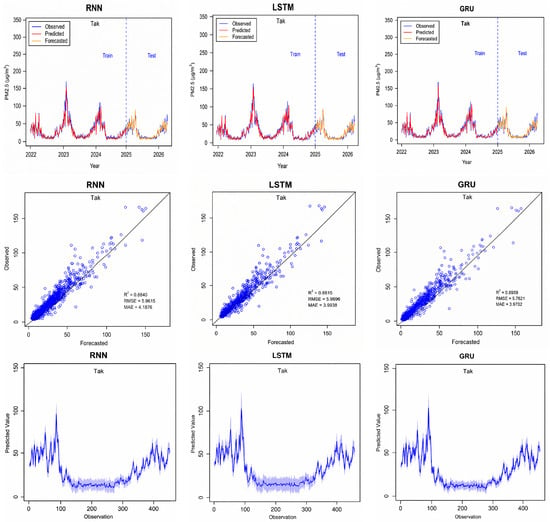
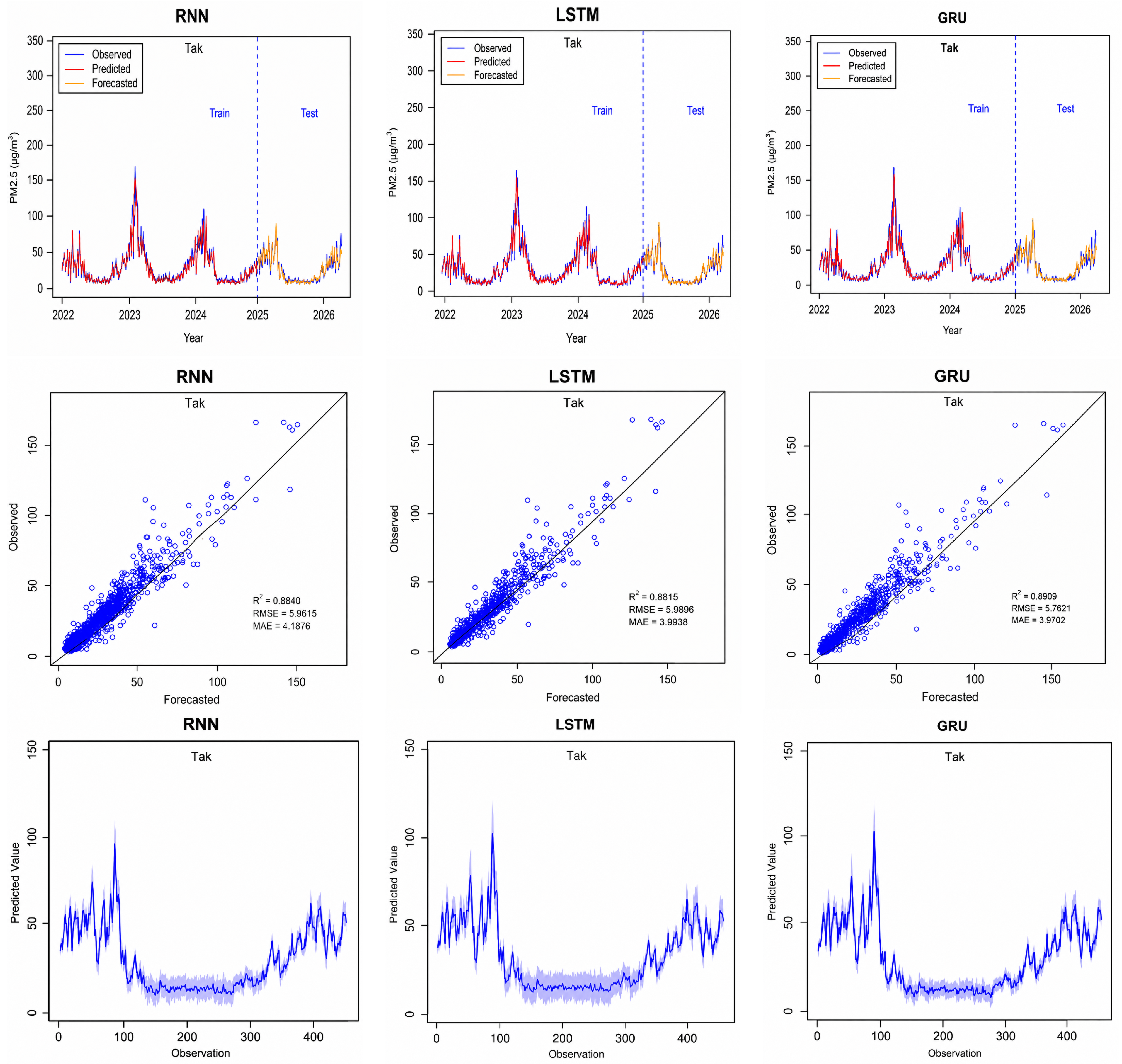
For Tak, the GRU model demonstrates marginally stronger predictive performance than the other evaluated models, achieving the best error metrics (, and ). The Diebold–Mariano test indicates statistically significant differences in predictive accuracy between the GRU and the RNN models under both squared-error and absolute-error loss functions (p-value ). The GRU and LSTM models are significantly different under the squared-error but not under the absolute-error loss, while the opposite is true for the comparison of the RNN and LSTM models.
concentrations exhibit substantial temporal variability and seasonal fluctuations, although extreme pollution episodes are generally less severe than those observed in Mae Hong Son and Lampang. As illustrated in Figure 8, the predicted series from all three models closely follow the observed dynamics during both the training and test periods, with only minor visual differences among the models. The regression curves of observed versus predicted values for one-day-ahead forecasting show relatively tight clustering around the reference line, indicating stable predictive performance. The confidence interval bands in Tak remain relatively consistent across all models, reflecting stable forecasting behaviour under less extreme temporal variability. Although the differences are visually subtle, the GRU model exhibits marginally narrower bands during several high-concentration periods.
Figure 8.
Performance of the RNN, LSTM, and GRU models for one-day-ahead forecasting in Tak. The top-row panels show the observed and predicted (µg/m3) time series; the middle-row panels show observed versus forecasted (µg/m3) values; and the bottom-row panels show the confidence interval bands of the predicted values based on 500 replications.
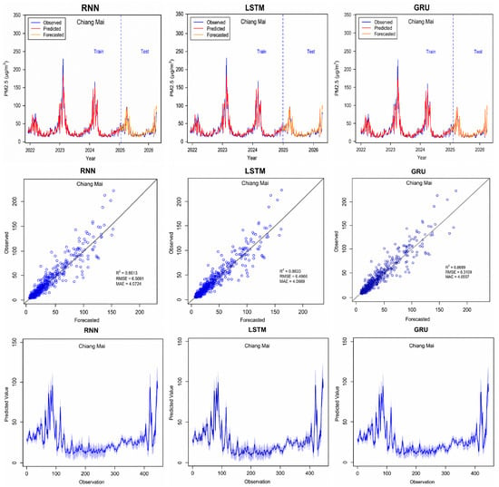
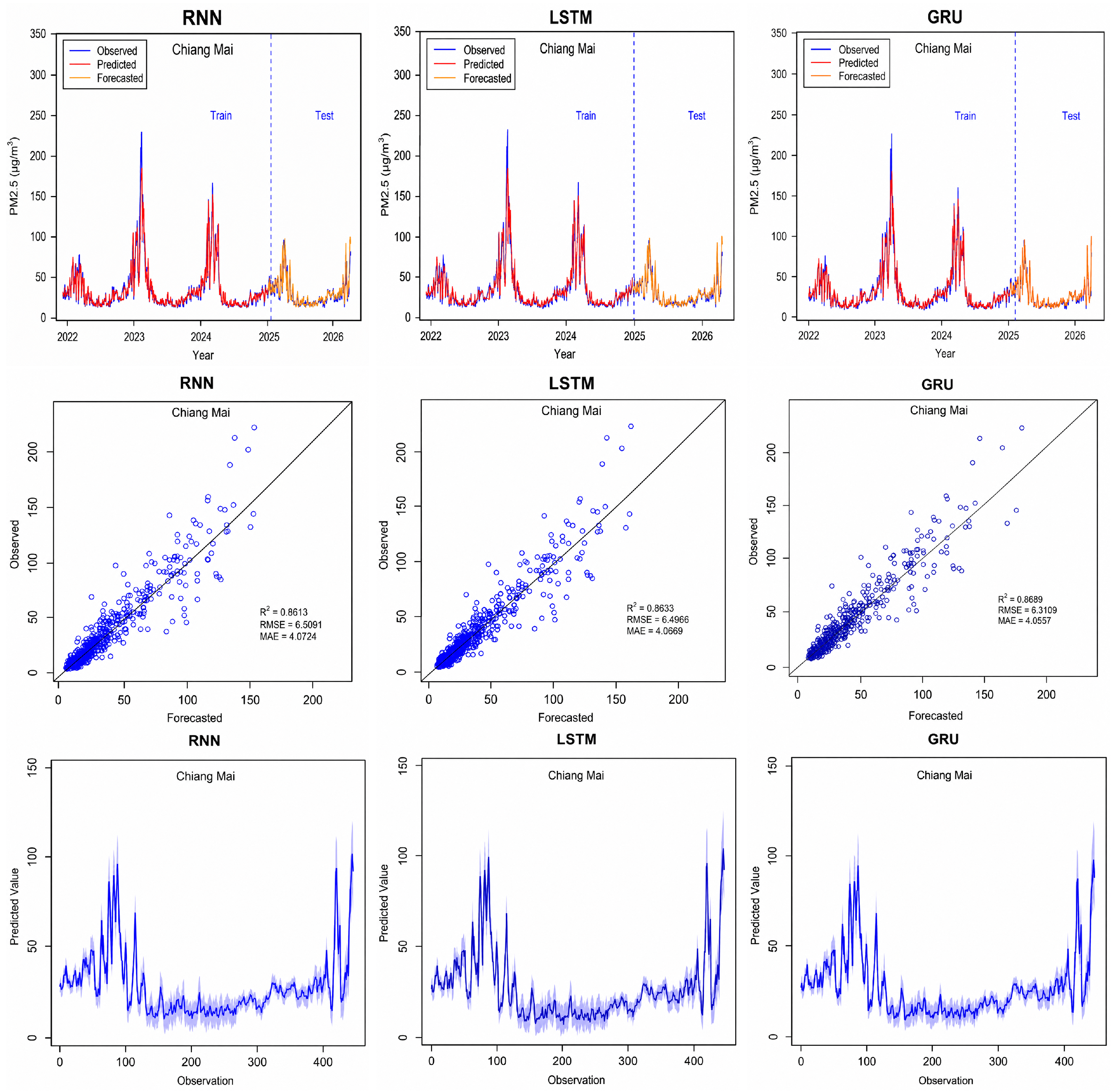
Chiang Mai also exhibits a clear seasonal structure consistent with the other northern provinces. Consistent with the performances observed for Lampang and Tak, the GRU model here is again the best model based on the three evaluation metrics. However, here the Diebold–Mariano test indicates no statistically significant differences in predictive accuracy. Overall, these results suggest relatively comparable predictive capability among the models under the temporal characteristics of this province.
Figure 9 illustrates close agreement between observed and predicted trajectories across both the training and test periods in Chiang Mai. Nevertheless, some underestimation remains during high episodes. The regression curves of observed versus predicted values for one-day-ahead forecasting exhibit increased dispersion at higher concentration levels, indicating greater forecasting uncertainty during severe pollution conditions. Compared with Mae Hong Son, Chiang Mai exhibits generally smoother temporal variability, indicating noticeably more stable forecasting behaviour across all models. In Chiang Mai, the confidence interval bands remain relatively stable across the forecasting horizon, suggesting consistent model generalisation under moderate temporal variability. The GRU model produces comparatively narrower bands than the other models, indicating reduced predictive fluctuation across repeated simulations.
Figure 9.
Performance of the RNN, LSTM, and GRU models for one-day-ahead forecasting in Chiang Mai. The top-row panels show the observed and predicted (µg/m3) time series; the middle-row panels show observed versus forecasted (µg/m3) values; and the bottom-row panels show the confidence interval bands of the predicted values based on 500 replications.
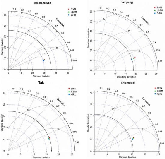
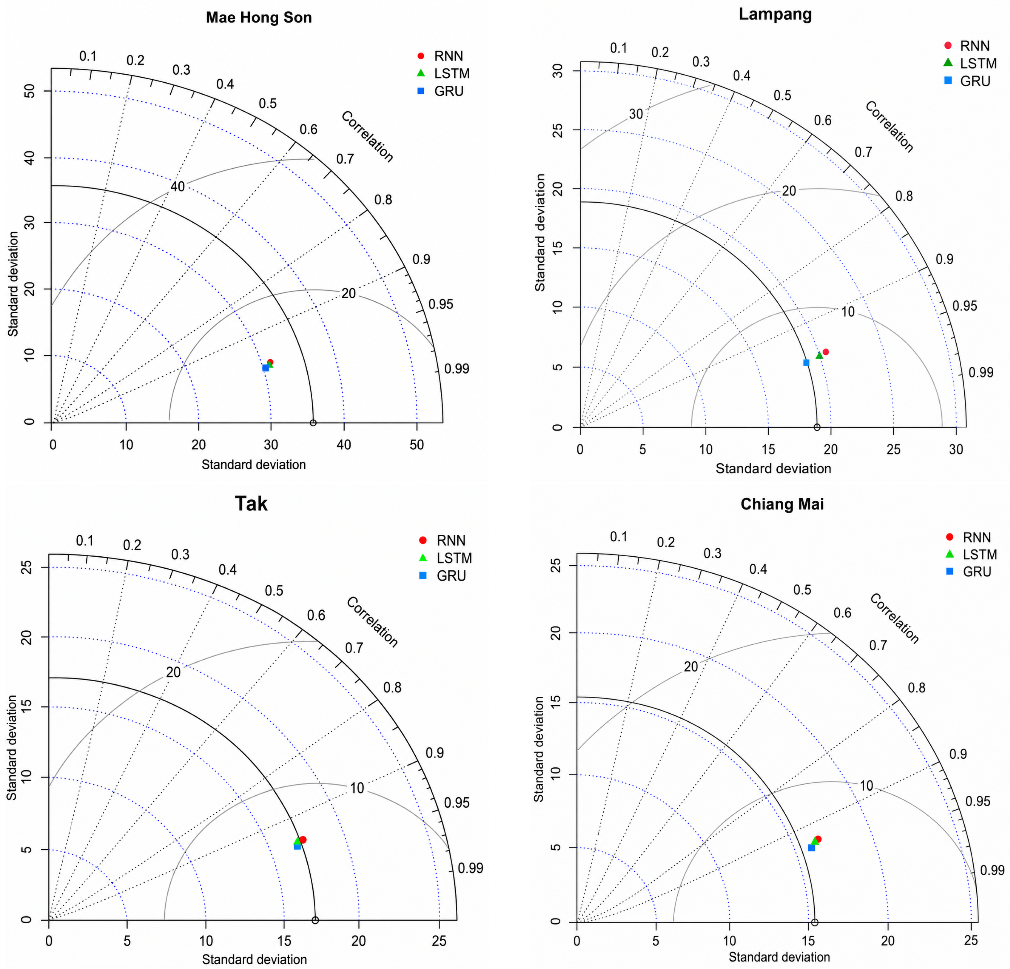
The Taylor diagrams in Figure 10 summarise the high correlation between observed and forecasted values across all models and regions. The standard deviations of all models are consistent with those of the observations, although there is a small underestimation for Mae Hong Son. The model points are closely clustered across all four provinces, suggesting broadly comparable performance, although GRU and LSTM appear slightly closer to the observed reference point in some provinces. No single model clearly dominates across all locations based on the Taylor diagrams alone.
Figure 10.
Taylor diagram summarising correlation, standard deviation (µg/m3), and centred RMSE for RNN, LSTM, and GRU forecasts across the four provinces, relative to observed concentrations.
Overall, the forecasting performance of the recurrent architectures depends strongly on the volatility and temporal characteristics of the underlying series. The GRU model demonstrates greater robustness under highly nonstationary conditions, whereas performance differences among models become less pronounced in provinces with comparatively smoother temporal dynamics. Practitioners may therefore find the GRU architecture preferable when local series are characterised by high temporal variability and frequent abrupt peaks, while the standard RNN offers comparable accuracy at a lower computational cost in more stable environments. It is worth noting that model performance was evaluated under hindcast conditions using observed values. The use of predicted values as model inputs would introduce additional uncertainty not reflected in the reported metrics.
4. Discussion
The present study focuses on one-day-ahead forecasting of daily average concentrations. Although hourly observations can capture within-day variability and diurnal patterns, aggregation to a 24 h average smooths short-term fluctuations and therefore does not explicitly represent the diurnal cycle or transient hourly pollution peaks. Accordingly, the findings discussed below should be interpreted specifically in the context of daily-scale forecasting, rather than as a characterisation of sub-daily air quality dynamics.
The deep learning models, particularly the GRU architecture, demonstrate the strongest one-day-ahead forecasting performance for concentrations, as summarised in Table 6 (derived from Table 4 and Table 5). The magnitude of the GRU’s advantage over the standard RNN is not constant across provinces: it is largest in Mae Hong Son, where GRU reduces MAE by 14.4% relative to RNN (4.7100 vs. 5.5031 µg/m3), moderate in Lampang (9.5% reduction; 3.6292 vs. 4.0089 µg/m3) and Tak (5.2% reduction; 3.9702 vs. 4.1876 µg/m3), and negligible in Chiang Mai (0.4% reduction; 4.0557 vs. 4.0724 µg/m3). This ordering mirrors the relative volatility of the four provinces, with Mae Hong Son exhibiting the most extreme and rapidly changing episodes and Chiang Mai the most stable dynamics (see Table 2 and Figure 3).
Table 6.
Summary of best-performing model per evaluation metric and the relative improvement of GRU over the standard RNN (based on Table 4), ordered by decreasing volatility.
The Diebold–Mariano test results in Table 5 support this pattern. Under the absolute-error loss, GRU significantly outperforms RNN in Mae Hong Son (, p-value < ), Lampang (, p-value = ), and Tak (, p-value = ) but shows no significant difference in Chiang Mai (, p-value = ). The comparison between LSTM and GRU is less pronounced, being significant only in Lampang and Tak under the squared-error loss function (, p-value = and , p-value = , respectively), with no significant difference in Chiang Mai. This indicates that while GRU reliably improves on the plain RNN in volatile regimes, its advantage over LSTM specifically is more limited and province-dependent (consistent with Park et al. [10] and Wongrin et al. [32], who report similar gains for gated architectures under nonlinear and nonstationary conditions). In Chiang Mai, the standard RNN remains competitive across all three evaluation metrics, while the DM tests confirm no significant pairwise differences among any of the three models, suggesting that in comparatively stable temporal regimes, the added architectural complexity of gated units yields little measurable benefit, aligned with the findings of Ayturan et al. [18].
While the deep learning models demonstrate strong forecasting performance, it is important to note that the models were trained using historical data, consistent with the work of Wongrin et al. [32]. In addition to model architecture, the forecasting performance was also influenced by the selected temporal input structure. A lag-1 input structure was selected to capture the dominant short-term temporal dependence in and to avoid unnecessary model complexity, which agrees with the work of Zaini et al. [24]. Although longer lag structures may provide additional temporal information, they may also introduce noise and increase the risk of overfitting, particularly in highly nonlinear and nonstationary environments, in agreement with the findings of Rutyna, I. [46].
Model performance tends to decrease during the dry season, when biomass burning and long-range pollutant transport contribute to highly variable concentrations and abrupt extreme peaks, similar to findings reported by Pak et al. [12] and Thaweephol and Wiwatwattana [31]. In this regime, all models tend to underestimate extreme concentration levels, indicating limitations in capturing sudden emission-driven events. These forecasting differences may reflect the greater temporal variability and increased pollution instability observed during the dry season. These findings suggest that model accuracy is strongly regime-dependent and highlight the importance of incorporating seasonal or process-based information in future forecasting frameworks.
The performance differences observed across provinces are consistent with their distinct physical settings described in Section 2.1. Mae Hong Son and Tak, both bordering Myanmar and confined by mountain valley topography that limits pollutant dispersion, exhibit the highest variability (Table 2) and are also where the GRU’s improvement over the standard RNN is largest (Table 6). This is consistent with these two provinces being most exposed to long-range, transboundary transport of smoke, a process governed substantially by wind direction and regional atmospheric circulation, neither of which is included in the current predictor set. Wind speed alone captures the intensity of local mixing and dispersion but cannot indicate whether incoming air is importing pollution from active fire regions upwind or clean air from an unaffected direction. This omission is a plausible explanation for the systematic underestimation of extreme peaks noted earlier in Mae Hong Son and Tak; without knowledge of wind direction, none of the three architectures can anticipate a transboundary smoke incursion before it manifests directly in the series itself and can only react to it one step after it appears in the lagged input.
By contrast, Chiang Mai, whose profile combines local agricultural and urban sources within a broader basin rather than being dominated by cross-border transport, shows the lowest variability of the four provinces. Under these more stable conditions, the RNN, LSTM, and GRU models deliver comparable forecasting performance (Table 5). It can therefore be inferred that where local sources dominate over long-range transport, the temporal dynamics captured by a lag-1 structure and locally observed meteorology appear largely sufficient, and the added gating mechanisms of the LSTM and GRU provide little additional benefit. Lampang falls between these two regimes; it is less directly exposed to transboundary transport than Mae Hong Son or Tak but still experiences substantial local and regional biomass burning, consistent with its intermediate variability and its intermediate (but still statistically significant) GRU improvement over RNN (9.5% MAE reduction, Table 6).
Altogether, these results suggest that the value of gated recurrent architectures over the standard RNN is not universal but depends on the extent to which a province’s dynamics are governed by transboundary, wind-direction-dependent transport rather than by local, more temporally regular sources. Models that explicitly incorporate wind direction, together with satellite- or reanalysis-derived indicators of long-range transport, such as air-mass back trajectories and transboundary fire-count indices, would be able to anticipate, rather than only react to, incoming pollution episodes and represent the most direct route to improving forecasting performance, specifically in the provinces where the current models perform least reliably. Furthermore, forecasting accuracy may be enhanced by integrating information from neighbouring monitoring stations using spatiotemporal deep learning architectures that jointly model both temporal and spatial dependencies.
5. Conclusions
For all forecasting models, a lag-1 input structure was selected based on the PACF analysis to provide a parsimonious and consistent framework across provinces. The hyperparameters of the RNN, LSTM, and GRU models were optimised using a grid search and cumulative (expanding-window) rolling cross-validation, and the final configurations were selected to balance forecasting accuracy, training stability, and forecasting robustness. The experimental results demonstrate that the GRU model provides more robust one-day-ahead forecasting performance under highly volatile and nonstationary conditions. Specifically, the GRU is preferable when the local series exhibits frequent abrupt peaks and strong regime-switching behaviour, whereas performance differences among the recurrent architectures become less pronounced under comparatively smoother temporal conditions. The LSTM model demonstrates competitive performance across all provinces but does not consistently outperform either alternative. These results indicate that the choice of recurrent architecture should be guided by the temporal volatility of the target environment rather than by architectural complexity alone.
As noted in Section 4, this study has several limitations that should be acknowledged. First, wind direction was excluded from the meteorological predictor set because of data incompleteness and the added complexity of circular variable encoding, which may limit the models’ ability to capture transboundary transport effects known to influence in the region. Second, the proposed models produce point forecasts and do not explicitly quantify predictive uncertainty in a probabilistic manner, even though confidence bands were examined through repeated simulations. Third, spatial dependencies, such as neighbouring monitoring station data, satellite-derived variables, or regional atmospheric circulation, were not explicitly modelled, despite their relevance to dynamics in northern Thailand. Fourth, because model training relies on an MSE-based loss function, all three architectures systematically underestimate extreme pollution peaks, which is particularly consequential for early-warning applications where correctly capturing extremes is often more important than minimising average error. The models’ implicit assumption that day ()’s meteorology is a reasonable proxy for day t is another potential source of this underestimation, particularly in provinces exposed to fast-moving transboundary smoke events. Adapting the current framework to redress this requires forecasting the meteorological predictors and introduces an additional source of error not present in the current design.
Despite its limitations, this study highlights the practical applicability of GRU-based frameworks for short-term air quality prediction in northern Thailand and provides a methodological baseline for future development of advanced deep learning and hybrid forecasting approaches. Future work may extend the analysis to transformer-based, convolutional, or ensemble forecasting models and could address the identified limitations by incorporating spatiotemporal dependencies, satellite-derived variables, and probabilistic forecasting methods. Future studies could also extend the proposed framework to hourly-resolution forecasting to explicitly characterise diurnal variability and short-term PM2.5 dynamics. Promising directions for addressing the systematic underestimation of extreme pollution peaks also include asymmetric or quantile-based loss functions that penalise underprediction more heavily than overprediction, and the replacement of the standard MSE output layer with a parametric extreme value distribution estimated directly through the network’s training objective. Beyond methodological contributions, this study also supports the broader framework of the United Nations Sustainable Development Goals (SDGs), particularly SDG 3 (Good Health and Well-being) and SDG 11 (Sustainable Cities and Communities). Accurate short-term forecasting of concentrations can support early-warning systems, public health risk communication, and air quality management strategies in regions frequently affected by severe haze pollution. By improving short-term forecasting capability under highly volatile and nonstationary conditions, the proposed deep learning framework may contribute to reducing pollution exposure, supporting evidence-based environmental policy, and strengthening environmental resilience in pollution-prone regions.
Supplementary Materials
The following supporting information can be downloaded at https://www.mdpi.com/article/10.3390/forecast8050080/s1, Figure S1. Recurrent architectures used in this study.
Author Contributions
Conceptualisation, N.J. and S.S.; methodology, N.J. and S.S.; software, N.J. and S.S.; validation, N.J., S.S. and M.F.B.; formal analysis, N.J., S.S. and M.F.B.; resources, S.S.; data curation, N.J. and S.S.; writing—original draft preparation, S.S.; writing—review and editing, N.J. and S.S.; visualisation, N.J. and S.S.; supervision, S.S.; project administration, S.S. All authors have read and agreed to the published version of the manuscript.
Funding
This research was supported by Walailak University International Mobility for Publication and Collaboration funding by grant number WU-CIA06106/2025.
Institutional Review Board Statement
Not applicable.
Informed Consent Statement
Not applicable.
Data Availability Statement
The datasets on concentrations are publicly available from the websites of the Pollution Control Department, Ministry of Natural Resources and Environment of Thailand, at http://air4thai.pcd.go.th/webV3/#/History (accessed on 24 August 2026), and the Air Quality and Noise Management Bureau, Ministry of Natural Resources and Environment of Thailand, at https://pm25.gistda.or.th/download (accessed on 24 August 2026). Meteorological variables were obtained from the websites of the Meteorological Information Subdivision, Northern Meteorological Center, Thai Meteorological Department, at https://cmmet.tmd.go.th/forecast/pt/pt_Data/Northern_Metdata.php (accessed on 24 August 2026), and the Thai Meteorological Department Automatic Weather System at http://www.aws-observation.tmd.go.th (accessed on 24 August 2026).
Acknowledgments
We would like to thank the Pollution Control Department, Air Quality and Noise Management Bureau, Ministry of Natural Resources and Environment of Thailand and Northern Meteorological Center of Thailand for providing the valuable data used in this study.
Conflicts of Interest
The authors declare no conflicts of interest.
Abbreviations
The following abbreviations are used in this manuscript:
| PM | Particulate matter |
| WHO | World Health Organization |
| ML | Machine learning |
| DL | Deep learning |
| RNN | Recurrent neural network |
| LSTM | Long short-term memory |
| GRU | Gated recurrent unit |
| Coefficient of determination | |
| Root mean square error | |
| Mean absolute error | |
| SVMs | Support vector machines |
| RF | Random forests |
| ANNs | Artificial neural networks |
| XGBoost | Extreme gradient boosting |
| CNNs | Convolutional neural networks |
| BiLSTM | Bi-directional long short-term memory |
| AQI | Air quality index |
| ARIMA | Autoregressive integrated moving average |
| GISTDA | Geo-Informatics and Space Technology Development Agency (Public Organisation) |
| RNNs | Recurrent neural networks |
| PACF | Partial autocorrelation functions |
| ACF | Autocorrelation functions |
| RMSprop | Root mean square propagation |
| MSE | Mean squared error |
| SDGs | Sustainable Development Goals |
References
- World Health Organization (WHO). World Health Statistics. Available online: https://www.who.int/data/gho/publications/world-health-statistics (accessed on 12 August 2025).
- Shu, X.; Cao, J.; Liu, Q.; Wang, Y.; Jiang, F.; Wu, C.; Shu, J. Global trends and hotspots in the research of the effects of PM2.5 on asthma: A bibliometric and visualized analysis. Epidemiol. Glob. Health 2024, 14, 1720–1736. [Google Scholar] [CrossRef] [Scilit] [PubMed]
- Dong, L.; Hua, P.; Gui, D.; Zhang, J. Extraction of multi-scale features enhances the deep learning-based daily PM2.5 forecasting in cities. Chemosphere 2022, 308, 136252. [Google Scholar] [CrossRef] [Scilit] [PubMed]
- Ma, X.; Chen, T.; Ge, R.; Xv, F.; Cui, C.; Li, J. Prediction of PM2.5 concentration using spatiotemporal data with machine learning models. Atmosphere 2022, 14, 1517. [Google Scholar] [CrossRef] [Scilit]
- World Health Organization (WHO). What Are Health Consequences of Air Pollution on Populations. Available online: https://www.who.int/news/item/25-06-2024-what-are-health-consequences-of-air-pollution-on-populations (accessed on 12 August 2025).
- Joharestani, M.Z.; Cao, C.; Ni, X.; Bashir, B.; Talebiesfandarani, S. PM2.5 prediction based on random forest, XGBoost, and deep learning using multisource remote sensing data. Atmosphere 2019, 10, 373. [Google Scholar] [CrossRef] [Scilit]
- Inlaung, K.; Chotamonsak, C.; Macatangay, R.; Surapipith, V. Assessment of transboundary PM2.5 from biomass burning in Northern Thailand using the WRF-Chem model. Toxics 2024, 12, 462. [Google Scholar] [CrossRef] [Scilit] [PubMed]
- Rocket Media Lab. The 5 Northern Provinces with the Largest Areas of Forest Fires. Available online: https://www.lannernews.com/18022568-01/ (accessed on 6 December 2025).
- Masood, A.; Ahmad, K. Data-driven predictive modeling of PM2.5 concentrations using machine learning and deep learning techniques: A case study of Delhi, India. Environ. Monit. Assess. 2023, 195, 60. [Google Scholar] [CrossRef] [Scilit] [PubMed]
- Park, S.-Y.; Woo, S.-H.; Lim, C. Predicting PM10 and PM2.5 concentration in container ports: A deep learning approach. Transp. Res. Part D 2023, 115, 103601. [Google Scholar] [CrossRef] [Scilit]
- Nguyen, P.H.; Dao, N.K.; Nguyen, L.S.P. Development of machine learning and deep learning prediction models for PM2.5 in Ho Chi Minh City, Vietnam. Atmosphere 2024, 15, 1163. [Google Scholar] [CrossRef] [Scilit]
- Pak, U.; Son, Y.; Kim, K.; Kim, J.; Jang, M.; Kim, K.; Pak, G. Novel particulate matter (PM2.5) forecasting method based on deep learning with suitable spatiotemporal correlation analysis. J. Atmos. Sol.-Terr. Phys. 2024, 264, 106336. [Google Scholar] [CrossRef] [Scilit]
- Liu, K.; Zhang, Y.; He, H.; Xiao, H.; Wang, S.; Zhang, Y.; Li, H.; Qian, X. Time series prediction of the chemical components of PM2.5 based on a deep learning model. Chemosphere 2023, 342, 140153. [Google Scholar] [CrossRef] [Scilit] [PubMed]
- Mohammadi, F.; Teiri, H.; Hajizadeh, Y.; Abdolahnejad, A.; Ebrahimi, A. Prediction of atmospheric PM2.5 level by machine learning techniques in Isfahan, Iran. Sci. Rep. 2024, 14, 2109. [Google Scholar] [CrossRef] [Scilit] [PubMed]
- Hochreiter, S.; Schmidhuber, J. Undersuchungen zu Dynamischen Neuronalen Netzen. Diploma Thesis, Technical University of Munich, Munich, Germany, 1991. [Google Scholar]
- Hochreiter, S.; Schmidhuber, J. Long short-term memory. Neural Comput. 1997, 9, 1735–1780. [Google Scholar] [CrossRef] [Scilit] [PubMed]
- Dey, R.; Salem, F.M. Gate-variants of gated recurrent unit (GRU) neural networks. In Proceedings of the 60th IEEE International Midwest Symposium on Circuits and Systems (MWSCAS), Boston, MA, USA, 6–9 August 2017; pp. 1597–1600. [Google Scholar]
- Ayturan, Y.A.; Ayturan, Z.C.; Altun, H.O.; Kongoli, C.; Tuncez, F.D.; Dursun, S.; Ozturk, A. Short-term prediction of PM2.5 pollution with deep learning methods. Glob. NEST J. 2020, 22, 126–131. [Google Scholar] [CrossRef] [Scilit]
- Pak, U.; Ma, J.; Ryu, U.; Ryom, K.; Juhyok, U.; Pak, K.; Pak, C. Deep learning-based PM2.5 prediction considering the spatiotemporal correlations: A case study of Beijing, China. Sci. Total Environ. 2020, 699, 133561. [Google Scholar] [CrossRef] [Scilit] [PubMed]
- Xiao, F.; Yang, M.; Fan, H.; Fan, G.; Al-qaness, M.A.A. An improved deep learning model for predicting daily PM2.5 concentration. Sci. Rep. 2020, 10, 20988. [Google Scholar] [CrossRef] [Scilit] [PubMed]
- Yang, J.; Yan, R.; Nong, M.; Liao, J.; Li, F.; Sun, W. PM2.5 concentrations forecasting in Beijing through deep learning with different inputs, model structures and forecast time. Atmos. Pollut. Res. 2021, 12, 101168. [Google Scholar] [CrossRef] [Scilit]
- Yeo, I.; Choi, Y.; Lops, Y.; Sayeed, A. Efficient PM2.5 forecasting using geographical correlation based on integrated deep learning algorithms. Neural Comput. Appl. 2021, 33, 15073–15089. [Google Scholar] [CrossRef] [Scilit]
- Li, D.; Liu, J.; Zhao, Y. Forecasting of PM2.5 concentration in Beijing using hybrid deep learning framework based on attention mechanism. Appl. Sci. 2022, 12, 11155. [Google Scholar] [CrossRef] [Scilit]
- Zaini, N.; Ean, L.W.; Ahmed, A.N.; Malek, M.A.; Chow, M.F. PM2.5 forecasting for an urban area based on deep learning and decomposition method. Sci. Rep. 2022, 12, 17565. [Google Scholar] [CrossRef] [Scilit] [PubMed]
- Cui, B.; Liu, M.; Li, S.; Jin, Z.; Zeng, Y.; Lin, X. Deep learning methods for atmospheric PM2.5 prediction: A comparative study of transformer and CNN-LSTM-attention. Atmos. Pollut. Res. 2023, 14, 101833. [Google Scholar] [CrossRef] [Scilit]
- Suriya; Natsagdorj, N.; Aorigele; Zhou, H.; Sachurila. Prediction of PM2.5 concentration in Ulaanbaatar with deep learning models. Urban Clim. 2023, 47, 101357. [Google Scholar] [CrossRef] [Scilit]
- Wu, K.-Y.; Hsia, I.-W.; Kow, P.-Y.; Chang, L.-C.; Chang, F.-J. High-spatiotemporal-resolution PM2.5 forecasting by hybrid deep learning models with ensembled massive heterogeneous monitoring data. J. Clean. Prod. 2023, 433, 139825. [Google Scholar] [CrossRef] [Scilit]
- Srikamdee, S.; Onpans, J. Forecasting daily air quality in northern Thailand using machine learning techniques. In Proceedings of the 2019 4th International Conference on Information Technology (InCIT), Amman, Jordan, 3–5 June 2019; pp. 259–263. [Google Scholar]
- Punpukdee, P.; Winijkul, E.; Kyaw, P.P.; Virdis, S.G.P.; Xue, W.; Nguyen, T.P.L. Estimation of hourly one square kilometer fine particulate matter concentration over Thailand using aerosol optical depth. Front. Environ. Sci. 2024, 11, 1303152. [Google Scholar] [CrossRef] [Scilit]
- Kawichai, S.; Sripan, P.; Rerkasem, A.; Rerkasem, K.; Srisukkham, W. Long-term retrospective predicted concentration of PM2.5 in upper northern Thailand using machine learning models. Toxics 2025, 13, 170. [Google Scholar] [CrossRef] [Scilit] [PubMed]
- Thaweephol, K.; Wiwatwattana, N. Long short-term memory deep neural network model for PM2.5 forecasting in the Bangkok urban area. In Proceedings of the 17th International Conference on Knowledge Engineering (ICT&KE), Bangkok, Thailand, 20–22 November 2019; pp. 1–6. [Google Scholar]
- Wongrin, W.; Chaisee, K.; Suphawan, K. Comparison of statistical and deep learning methods for forecasting PM2.5 concentration in northern Thailand. Pol. J. Environ. Stud. 2023, 32, 1419–1431. [Google Scholar] [CrossRef] [Scilit] [PubMed]
- Laohakiat, S.; Klerkkidakan, S.; Wiwatwattana, N. Visually estimating and forecasting PM2.5 levels using hybrid architecture deep neural network. Curr. Appl. Sci. Technol. 2023, 24, e0258074. [Google Scholar] [CrossRef] [Scilit]
- Damkliang, K.; Chumnaul, J. Deep learning and statistical approaches for area-based PM2.5 forecasting in Hat Yai, Thailand. J. Big Data 2025, 12, 36. [Google Scholar] [CrossRef] [Scilit]
- Kaewbundit, V.; Churngam, C.; Wongchaisuwat, P. A spatiotemporal deep learning ensemble for multi-step PM2.5 prediction: A case study of Bangkok metropolitan region in Thailand. Atmos. Pollut. Res. 2025, 16, 102406. [Google Scholar] [CrossRef] [Scilit]
- Air Quality and Noise Management Bureau, Ministry of Natural Resources and Environment of Thailand. Archived Data of the Daily Average PM2.5 Concentration. Available online: http://air4thai.pcd.go.th/webV3/#/History (accessed on 7 April 2026).
- Geo-Informatics and Space Technology Development Agency. The PM2.5 Database System. Available online: https://pm25.gistda.or.th/download (accessed on 7 April 2026).
- Northern Meteorological Center. Meteorological Information Service. Available online: https://cmmet.tmd.go.th/forecast/pt/pt_Data/Northern_Metdata.php (accessed on 8 April 2026).
- Thai Meteorological Department Automatic Weather System. Search of Past Data of Climate Data. Available online: http://www.aws-observation.tmd.go.th (accessed on 8 April 2026).
- QGIS Geographic Information System, Version 4.0, Open Source Geospatial Foundation Project. 2026. Available online: http://qgis.org (accessed on 17 April 2026).
- Thailand-Subnational Administrative Boundaries. OCHA Services. Available online: https://data.humdata.org/dataset/cod-ab-tha (accessed on 17 April 2026).
- James, G.; Witten, D.; Hastie, T.; Tibshirani, R. An Introduction to Statistical Learning: With Applications in R, 2nd ed.; Springer: New York, NY, USA, 2023. [Google Scholar]
- Elsworth, S.; Güttel, S. Time series forecasting using LSTM networks: A symbolic approach. arXiv 2020, arXiv:2003.05672. [Google Scholar]
- Diebold, F.X.; Mariano, R.S. Comparing predictive accuracy. J. Bus. Econ. Stat. 1995, 13, 253–263. [Google Scholar] [CrossRef] [Scilit]
- Graham, J.W. Missing data analysis: Making it work in the real world. Annu. Rev. Psychol. 2009, 60, 549–576. [Google Scholar] [CrossRef] [Scilit] [PubMed]
- Rutyna, I. Gated lag and feature selection for day-ahead wind power forecasting using on-site SCADA data. Wind 2025, 4, 28. [Google Scholar] [CrossRef] [Scilit]

Disclaimer/Publisher’s Note: The statements, opinions and data contained in all publications are solely those of the individual author(s) and contributor(s) and not of MDPI and/or the editor(s). MDPI and/or the editor(s) disclaim responsibility for any injury to people or property resulting from any ideas, methods, instructions or products referred to in the content. |
© 2026 by the authors. Licensee MDPI, Basel, Switzerland. This article is an open access article distributed under the terms and conditions of the Creative Commons Attribution (CC BY) license.