Heterogeneous-Horizon Conformal Ensembles for Online Prediction Under Distribution Shift: An Empirical Comparison with Strongly Adaptive Methods

Highlights

What are the main findings?

• PACE improves extreme-regime coverage over five adaptive conformal baselines across all five evaluated datasets.
• PACE and Strongly Adaptive Online Conformal Prediction (SAOCP), a benchmark that combines calibration experts across multiple time intervals, have comparable coverage overall. PACE usually uses wider intervals and tends to perform relatively better as extreme events persist longer.

What are the implications of the main findings?

• Combining online conformal calibrators across multiple horizons is a practical way to reduce undercoverage during distribution shifts.
• PACE is most appropriate when coverage is the main priority, whereas SAOCP remains preferable when interval sharpness and formal strongly adaptive guarantees are more important.

Abstract

Online conformal prediction methods such as Adaptive Conformal Inference (ACI) and Fully Adaptive Conformal Inference (FACI) adjust prediction intervals under distribution shift, but their calibration is based on a common stream of recent nonconformity scores. We introduce Population-based Adaptive Conformal Ensembles (PACE), a heuristic method that maintains online conformal quantile calibrators with different window sizes, decay rates, and quantile scales. PACE combines the best-calibrated members through fitness-weighted top-K averaging and periodically refreshes the population using clonal selection. For context, Strongly Adaptive Online Conformal Prediction (SAOCP) is a benchmark method that combines online calibration experts operating over different time intervals and provides a formal strongly adaptive regret guarantee. PACE is heuristic and does not provide an analogous regret or coverage guarantee. We evaluate the method on two synthetic datasets and three real-world time series. Against five adaptive conformal baselines, PACE achieves higher empirical coverage during extreme regimes. Compared with SAOCP, it generally obtains higher coverage by producing wider intervals, resulting in less favorable interval scores on most datasets.

1. Introduction

Conformal prediction provides distribution-free prediction intervals with finite-sample coverage guarantees when the observations are exchangeable [1,2]. In many applications, however, the data distribution changes over time. Financial markets move between calm and volatile periods, energy prices respond to shocks, climate series evolve, and sensor streams may drift or fail. Under such shifts, the classical exchangeability-based guarantee no longer applies. Adaptive Conformal Inference (ACI) [3] responds by updating the miscoverage level ${\alpha }_t$ online, while Fully Adaptive Conformal Inference (FACI) [4] combines updates at several learning rates. Both methods adapt using a shared stream of nonconformity scores and have established long-run coverage properties. More recent work studies a stronger form of adaptation, commonly described as strongly adaptive coverage. The aim is to control performance not only over the full data stream but also over every contiguous sub-interval. Bhatnagar et al. [5] develop two methods in this setting: Scale-Free Online Gradient Descent (SF-OGD) and Strongly Adaptive Online Conformal Prediction (SAOCP). SAOCP creates SF-OGD experts on dyadic active intervals and combines them using coin-betting weights, yielding an $\tilde{O}\left(\sqrt{k}\right)$ regret bound against any comparator on a contiguous window of length k. Because SAOCP couples online adaptation with a formal strongly adaptive guarantee, it serves as our primary comparator.

This paper investigates a different heuristic approach. We propose Population-based Adaptive Conformal Ensembles (PACE), which maintains a heterogeneous population of online quantile calibrators. Every member receives the same normalized nonconformity scores but uses its own window size $w_i$, decay rate ${\lambda }_i$, and quantile-scaling factor ${\kappa }_i$. At each step, PACE selects the members whose recent coverage is closest to the target and combines their quantiles through fitness-weighted top-K averaging. The population is periodically refreshed by replacing poorly calibrated members with mutated clones of stronger ones. PACE is not covered by existing strongly adaptive analyses, and we make no claim of a strongly adaptive regret or coverage guarantee.

The main motivation is that a single calibration horizon is unlikely to be appropriate throughout a non-stationary stream. Short windows can respond quickly after a regime change, but their estimates are variable. Longer windows are more stable, but they may react too slowly. PACE keeps calibrators at both short and long horizons available at the same time and changes their influence as their empirical calibration improves or deteriorates. SAOCP creates adaptivity along a different axis. It keeps a common scoring rule but varies the lifetime of its experts: new experts are introduced continually, and younger experts respond most strongly to the current regime. PACE instead uses a persistent population whose members have different response speeds. It does not recall old regimes in the sense of storing a library of past states. Its distinction is that it distributes calibration across several time scales.

1.1. Contributions

We make three contributions.

• We introduce PACE, a heuristic ensemble of online conformal quantile calibrators operating over heterogeneous horizons. On five datasets, PACE achieves higher empirical coverage during extreme regimes than ACI, FACI, PID-Conformal, AgACI, and SF-OGD.
• We provide preliminary evidence that the difference between PACE and SAOCP depends on event duration. Across retrospectively identified extreme regimes, the per-event coverage gap tends to move in favor of PACE as events become longer.
• We use ablation studies to examine the source of PACE’s gains. Removing clonal selection, top-K weighting, or quantile-scale diversity does not eliminate the improvement on its own.

1.2. Outline

Section 2 reviews related work and develops the comparison with SAOCP. Section 3 describes PACE. Section 4 presents the main experiments on five datasets, including the baseline comparison and event-duration analysis. Section 5 reports robustness studies, and Section 6 discusses limitations and open questions.

2. Related Work

2.1. Conformal Prediction and Exchangeability

Conformal prediction [1,2] provides distribution-free prediction sets with finite-sample coverage guarantees under the sole assumption that the data are exchangeable. Split conformal prediction [6] makes the framework computationally practical, and conformalized quantile regression [7] adapts intervals to heteroscedasticity. Angelopoulos and Bates [8] gives a modern overview. A key limitation is the reliance on exchangeability: when the data-generating distribution shifts, finite-sample coverage guarantees no longer hold. Barber et al. [9] generalizes to weighted exchangeability and Tibshirani et al. [10] addresses known covariate shift, but neither addresses the online setting with unknown recurring distributional changes.

2.2. Online Adaptive Conformal Inference

Gibbs and Candès [3] introduced ACI, which updates the target miscoverage level online via gradient descent. Gibbs and Candès [4] extended this to FACI, running multiple ACI experts at different learning rates and aggregating them via exponential weights. Zaffran et al. [11] proposed AgACI, a parameter-free aggregation of ACI instances using Bernstein Online Aggregation on lower and upper bounds separately. Angelopoulos et al. [12] drew an analogy with PID control, using proportional, integral, and derivative terms to adapt prediction intervals. All these methods maintain a single stream of nonconformity scores; when a previously visited regime recurs, the score window is overwritten, and the method must re-learn from scratch.

2.3. Strong Adaptation

Bhatnagar et al. [5] introduced SF-OGD and SAOCP, among the strongest online conformal methods for arbitrary distribution shift. SF-OGD is a Scale-Free Online Gradient Descent algorithm on the pinball quantile loss, with an anytime regret bound against any fixed comparator. SAOCP runs a logarithmic number of SF-OGD experts on dyadic active intervals: each expert is born at a given step, lives for a length that depends on how many times two divides that step, and is combined with the others through coin-betting weights, achieving a strongly adaptive regret bound on every contiguous interval. SAOCP is the leading comparator in this paper and the primary point of reference for PACE; we discuss the methodological relationship at length in Section 3.

2.4. Ensemble-Based Conformal Prediction for Time Series

A separate line of work uses ensembles of base predictors to construct conformal intervals. Xu and Xie [13] introduced EnbPI, which wraps around bootstrap ensemble estimators; Xu and Xie [14] extended this with SPCI. Stankeviciute et al. [15] proposed conformal forecasting RNNs. These methods ensemble the point-prediction step and then calibrate a single score; PACE, instead, ensembles the score computation and quantile estimation step. In a related direction, Millard et al. [16] extends split conformal prediction to function-valued outputs via neural operator learning.

2.5. Regime-Switching Models and Change-Point Detection

The challenge of recurring distributional regimes has a long history, beginning with Hamilton’s [17] Markov-switching model. Change point detection methods [18] and dependent-data conformal methods [19] address related problems, but they either assume a parametric regime structure or focus on detecting single change points. PACE uses a lightweight heuristic regime detector to gate an optional memory-recall mechanism, deliberately avoiding strong parametric assumptions.

2.6. Evolutionary and Immune-Inspired Algorithms

PACE’s population-level dynamics draw on the artificial immune systems literature, particularly the clonal selection algorithm [20,21]. The ensemble literature has long established that diversity among members is key to ensemble performance [22,23,24]. Hierarchical extensions of conformal prediction to multi-scale and multi-resolution settings are discussed in Baheri and Amiri Shahbazi [25], Amiri Shahbazi et al. [26]. PACE’s clonal-selection mechanism operationalizes the diversity principle for online conformal calibration.

3. Method

3.1. Setting and Notation

We work in the standard online conformal prediction framework. At each time t, the forecaster constructs a prediction interval $C_t\subseteq \mathbb{R}$ before observing the outcome $y_t$. The objective is to achieve the long-run coverage target

$$\underset{T\to \infty }{\lim \inf }{\displaystyle \frac{1}{T}}{\displaystyle \sum _{t=1}^T}\mathbf{1}[y_t\in C_t]\ge 1-\alpha ,$$

(1)

where $\alpha \in (0,1)$ denotes the target miscoverage rate. As in Gibbs and Candès [3], we do not require the observations to be exchangeable, and the data-generating process may change abruptly over time. Our main interest is in extreme-event regimes, in which a process that usually remains in a base regime occasionally enters one of several extreme states, such as a market crash, heatwave, or storm. These regimes may exhibit higher variance, heavier tails, or both. Accordingly, our primary evaluation metric is empirical coverage computed only over observations that belong to an extreme regime.

3.2. Shared Adaptive Location-Scale Normalization

To isolate differences in calibration, every method in the comparison, including all baselines, uses the same adaptive location-scale model to construct normalized nonconformity scores. At each step, the exponentially weighted location and scale estimates are updated according to

$${\widehat{\mu }}_{t\mid t-1}=(1-{\eta }_{\mu }){\widehat{\mu }}_{t-1\mid t-2}+{\eta }_{\mu }{y}_{t-1},{\widehat{\sigma }}_{t\mid t-1}^2=(1-{\eta }_{\sigma }){\widehat{\sigma }}_{t-1\mid t-2}^2+{\eta }_{\sigma }{(y_{t-1}-{\widehat{\mu }}_{t-1\mid t-2})}^2,$$

(2)

with smoothing rates ${\eta }_{\mu }=0.05$ and ${\eta }_{\sigma }=0.08$. The initial estimates are obtained from a calibration segment consisting of 150 observations for synthetic finance, 96 for synthetic energy, and between 50 and 250 for the real datasets. Given these estimates, the normalized nonconformity score is $s_t=|y_t-{\widehat{\mu }}_{t\mid t-1}|/{\widehat{\sigma }}_{t\mid t-1}$, and the corresponding prediction interval has the form

$$C_t=[{\widehat{\mu }}_{t\mid t-1}-q_t{\widehat{\sigma }}_{t\mid t-1},{\widehat{\mu }}_{t\mid t-1}+q_t{\widehat{\sigma }}_{t\mid t-1}],$$

(3)

where $q_t$ is a non-negative scalar determined entirely by previously observed scores. Thus, the methods differ only in the rule used to compute $q_t$, allowing the empirical comparison to focus on the effect of the calibration mechanism.

3.3. The PACE Method

PACE replaces ACI’s single quantile tracker with a population of $N=30$ score functions, $\mathcal{S}=\{S_1,\dots ,S_N\}$. Member $S_i$ is characterized by the parameter triple ${\theta }_i=(w_i,{\lambda }_i,{\kappa }_i)$, comprising a window size $w_i\in [10,150]$, a decay rate ${\lambda }_i\in [0.8,1.0]$, and a quantile-scaling factor ${\kappa }_i\in [0.5,1.8]$. At initialization, each parameter is sampled uniformly from its admissible range. The resulting variation across members provides the main source of diversity in the population.

3.3.1. Per-Member Quantile

Each member $S_i$ stores the most recent $\min (w_i,t-1)$ normalized scores. Scores within this buffer receive exponentially decaying weights: the score $s_{t-1-j}$ is assigned weight ${\omega }_j={\lambda }_i^j/{\sum }_{k=0}^{n-1}{\lambda }_i^k$. The raw weighted quantile ${\tilde{q}}_i^{\left(t\right)}$ is defined as the smallest score s for which the cumulative weight ${\sum }_{j:s_{t-1-j}\le s}{\omega }_j$ exceeds $1-\alpha$. The quantile reported by the member is

$${\widehat{q}}_i^{\left(t\right)}={\kappa }_i·{\tilde{q}}_i^{\left(t\right)},$$

(4)

so the factor ${\kappa }_i$ controls the scale of that member’s contribution to the final prediction interval.

3.3.2. Fitness Tracking

Each member measures its recent calibration through the exponential moving average $f_i^{\left(t\right)}=(1-{\eta }_f)f_i^{(t-1)}+{\eta }_f\mathbf{1}[s_t\le {\widehat{q}}_i^{\left(t\right)}]$, where ${\eta }_f=0.07$. Values of $f_i$ close to the target coverage level $1-\alpha$ indicate better empirical calibration.

3.3.3. Fitness-Weighted Top-K Aggregation

At each prediction step, PACE selects the $K=5$ members whose fitness values are closest to $1-\alpha$. Their quantiles are then combined using

$$q_t^{\mathrm{agg}}=\sum _{i\in \mathrm{top}\text{-}K}{\tilde{w}}_i·{\widehat{q}}_i^{\left(t\right)},{\tilde{w}}_i={\displaystyle \frac{{(|f_i-(1-\alpha )|+\epsilon )}^{-1}}{{\sum }_{j\in \mathrm{top}\text{-}K}{(|f_j-(1-\alpha )|+\epsilon )}^{-1}}},$$

(5)

where $\epsilon ={10}^{-3}$ is a regularization constant. PACE also applies a slowly varying multiplicative correction $c_t$, giving the prediction interval

$$C_t=[{\widehat{\mu }}_{t\mid t-1}-q_t^{\mathrm{agg}}{c}_t{\widehat{\sigma }}_{t\mid t-1},{\widehat{\mu }}_{t\mid t-1}+q_t^{\mathrm{agg}}{c}_t{\widehat{\sigma }}_{t\mid t-1}].$$

(6)

The correction is increased multiplicatively when rolling coverage falls below $0.88$ and decreased when it rises above $0.93$, with $c_t$ clipped to $[0.85,1.25]$. We use this global multiplicative adjustment instead of an ACI-style update to ${\alpha }_t$. Applying a common ${\alpha }_t$ update to every member would reduce the distinction among their calibration dynamics, whereas $c_t$ adjusts the overall interval width while preserving the member-specific effects of $(w_i,{\lambda }_i,{\kappa }_i)$. Equation (6) is therefore the PACE-specific counterpart of the generic interval in Equation (3), with the scalar $q_t$ replaced by $q_t^{\mathrm{agg}}{c}_t$.

3.3.4. Clonal Selection

Every $\mathsf{\Delta }=15$ step, the population is ranked by $|f_i-(1-\alpha )|$. The least well-calibrated third is replaced by mutated copies of the best-calibrated members. Each parameter is perturbed independently with Gaussian noise, using standard deviations 12, $0.02$, and $0.12$ for w, $\lambda$, and $\kappa$, respectively, and the resulting values are clipped to their admissible ranges. A child inherits the parent’s recent score history, truncated when necessary to match the child’s window size, along with a discounted version of the parent’s fitness. Algorithm 1 summarizes the complete procedure.

Algorithm 1 PACE: Population-based Adaptive Conformal Ensemble

Require: Miscoverage rate $\alpha$, population size N, top-K, selection interval $\mathsf{\Delta }$

1: Initialize $\mathcal{S}=\{S_1,\dots ,S_N\}$ with parameters drawn uniformly; initialize $c\leftarrow 1$   2: for $t=1,2,\dots$ do   3:       Stage 1 (Predict): compute ${\widehat{\mu }}_{t\mid t-1},{\widehat{\sigma }}_{t\mid t-1}$ via Equation (2)   4:       Select top-K members from $\mathcal{S}$ by minimal $|f_i-(1-\alpha )|$   5:       $q_t^{\mathrm{agg}}\leftarrow {\sum }_{i\in \mathrm{top}\text{-}K}{\tilde{w}}_i·{\widehat{q}}_i^{\left(t\right)}$                ▹ Equations (4) and (5)   6:       Output $C_t=[{\widehat{\mu }}_{t\mid t-1}\pm q_t^{\mathrm{agg}}·c·{\widehat{\sigma }}_{t\mid t-1}]$   7:       Stage 2 (Observe and score): observe $y_t$; compute $s_t=|y_t-{\widehat{\mu }}_{t\mid t-1}|/{\widehat{\sigma }}_{t\mid t-1}$   8:       Stage 3 (Update): for each $S_i\in \mathcal{S}$: append $s_t$ to buffer, update fitness $f_i$   9:       Update rolling coverage; adjust c 10:       if $t\mathrm{mod}\mathsf{\Delta }=0$ then 11:        Replace worst fraction in $\mathcal{S}$ with mutated clones of best members 12:       end if 13: end for

3.4. Relationship to SAOCP

PACE and the SAOCP method of Bhatnagar et al. [5] both combine multiple online quantile calibrators, but they introduce diversity along different dimensions. SAOCP keeps the scoring rule fixed, using SF-OGD to minimize pinball loss, and varies the lifetime of each expert. It creates a new expert at every step with an active interval length $g·2^{u\left(t\right)}$, where $u\left(t\right)$ is the largest power of two dividing t, and combines the active experts through coin-betting weights relative to a dyadic-interval prior. PACE instead keeps the basic estimation rule fixed, a weighted quantile computed from a recent score buffer, and varies the response speed through the member-specific window $w_i$ and decay rate ${\lambda }_i$. Its population persists over time and is gradually modified through clonal selection. The methods, therefore, respond to regime changes in different but complementary ways. SAOCP adapts by changing its active expert set, while PACE adjusts the influence of its existing heterogeneous population. This difference motivates the empirical analyses in Section 4.3, which compares their coverage, and Section 4.4, which studies how the coverage difference changes with the duration of a regime change.

4. Experiments

4.1. Setup

4.1.1. Methods

We evaluate PACE and its optional memory-augmented variant, PACE+M (reported in Table 1 and discussed in Section 4.8), alongside six baselines.

Table 1. Extreme-event coverage by method and dataset, in percent (target $1-\alpha =90$%). These values are from the main experiment suite. Synthetic-data entries are mean ± standard deviation across 20 seeds; real-data baselines are deterministic single runs (no standard deviation reported), while PACE and PACE+M on real data are mean ± standard deviation across 10 seeds. Independent robustness reruns in Section 5 use new random seeds and data-generation draws, so their absolute coverage values are not expected to reproduce this table. The best entry in each row is shown in bold. PACE dominates the five pre-SAOCP baselines on every dataset (all 25 pairwise tests significant at $p<0.05$, 22 at $p<0.001$); the head-to-head against SAOCP is summarized in Table 2.

Dataset	ACI	FACI	PID	AgACI	SF-OGD	SAOCP	PACE	PACE+M
Synth. Finance	$79.4\pm 4.2$	$81.5\pm 3.3$	$79.3\pm 4.7$	$81.4\pm 3.0$	$81.7\pm 2.1$	$\mathbf{85}.\mathbf{9}\pm \mathbf{2}.\mathbf{6}$	$85.1\pm 2.8$	$85.4\pm 2.5$
Synth. Energy	$87.7\pm 0.7$	$88.4\pm 0.6$	$89.8\pm 1.5$	$87.8\pm 1.1$	$88.9\pm 0.6$	$88.8\pm 0.9$	$\mathbf{90}.\mathbf{9}\pm \mathbf{1}.\mathbf{0}$	$90.5\pm 0.7$
S&P 500 (real)	$87.3$	$87.5$	$87.5$	$87.5$	$87.5$	$88.9$	$\mathbf{89}.\mathbf{1}\pm \mathbf{0}.\mathbf{9}$	$88.9\pm 0.4$
WTI Oil (real)	$85.8$	$86.3$	$85.6$	$86.8$	$86.1$	$\mathbf{88}.\mathbf{1}$	$87.3\pm 0.5$	$87.6\pm 0.6$
Sunspots (real)	$76.6$	$78.7$	$78.7$	$83.0$	$85.1$	$85.1$	$\mathbf{87}.\mathbf{5}\pm \mathbf{2}.\mathbf{0}$	$86.6\pm 2.1$

• ACI [3]: a single sliding-window method with an online update of ${\alpha }_t$.
• FACI [4]: a collection of multi-rate ACI experts combined through exponentially weighted aggregation.
• PID-Conformal [12]: a quantile-adjustment method based on proportional, integral, and saturating-derivative feedback.
• AgACI [11]: a BOA-style aggregation of ACI experts that applies pinball loss separately to the lower and upper bounds.
• SF-OGD [5]: Scale–Free Online Gradient Descent applied to the pinball quantile loss.
• SAOCP [5]: Strongly Adaptive Online Conformal Prediction using SF-OGD experts on dyadic intervals.

4.1.2. Datasets

The evaluation includes two synthetic and three real-world datasets selected to represent substantially different regime geometries:

• Synthetic Finance (1800 steps). The series consists of GARCH(1,1) returns divided into 15 regime-dependent segments. Three crash regimes, lasting $\{20,15,25\}$ days, have $55\%$ annualized volatility, Student-t innovations with $\nu =3$, and leverage effects. These extreme events are short relative to the score window. More precisely, the base process is $r_t={\sigma }_t{\epsilon }_t$, where ${\sigma }_t^2=\omega +a{r}_{t-1}^2+b{\sigma }_{t-1}^2$ and $(\omega ,a,b)=(0.05,0.08,0.90)$. Because $a+b<1$, the unconditional variance exists. The standardized Student-t innovations ${\epsilon }_t$ use $\nu =8$ in calm segments and the heavier-tailed value $\nu =3$ during crashes; crash segments also multiply the emitted return by an additional volatility factor. The resulting process captures volatility clustering, conditional heteroscedasticity, and heavy tails, three standard features of financial returns without imposing a closed-form marginal distribution.
• Synthetic Energy (1650 half-hours, or approximately 34 days). This series represents half-hourly demand for a regional grid operator and contains daily (48-step) and weekly (336-step) cycles. Its event schedule includes two heatwaves of 96 and 120 half-hours, two cold snaps of 96 and 72 half-hours, two storms of 36 and 48 half-hours, and one 24-step grid-stress event. These extreme events are long relative to the score window.
• S&P 500 (5030 days). We use daily log-returns from 5 January 1999 to 31 December 2018, as bundled with the arch package. The period covers the dot-com aftermath, the 2008 Global Financial Crisis, the 2010 flash crash, the 2015 China sell-off, and the 2018 “Volmageddon”. Extreme regimes are identified heuristically from the top-$10\%$ rolling-volatility decile using a 21-step window, yielding 22 regimes with a mean duration of $22.9$ steps and a range of $[2, 86]$.
• WTI Crude Oil (8320 days). The dataset contains daily log-returns from 1986 to 2019 and spans the 1990 Gulf War, the 1998 Asian crisis, the 2008 oil shock, and the 2014–2016 collapse. We identify 37 extreme regimes, with a mean duration of $19.1$ steps and a range of $[1, 154]$.
• Sunspots (309 years). This annual series covers the years 1700 to 2008. It includes the Dalton minimum (approximately 1790 to 1830) and the Modern Maximum (approximately 1950 to 2000). Defining extreme regimes through the top-$15\%$ rolling-volatility decile gives four regimes with a mean duration of $11.8$ years.

4.1.3. Protocol

All experiments set $\alpha =0.10$, corresponding to a target coverage of $90\%$. The calibration segments contain 150 observations for synthetic finance, 96 for synthetic energy, 250 for both S&P 500 and WTI, and 50 for sunspots. We evaluate PACE and PACE+M over 20 random seeds on the synthetic datasets and 10 seeds on the real datasets. The baselines are deterministic on the real datasets; where relevant, we report mean ± std and use one-sample t-tests against the PACE seed distribution when comparing PACE with a deterministic baseline. Two features of this protocol are important. First, every prediction is out-of-sample in the online sense. At time t, the interval $C_t$ is constructed only from observations available through $t-1$, and $y_t$ is revealed only after the interval has been fixed. The calibration segment is used exclusively to initialize the location-scale state and the score buffers; it is not reused for tuning, and no future observation contributes to an interval. We do not create a separate held-out test split because, under this online protocol, the full post-calibration stream already serves as a rolling out-of-sample test, as is standard in evaluations of adaptive conformal methods. Second, the datasets were chosen to cover a broad range of regime geometries. They include a short synthetic series with brief crashes (synthetic finance), a synthetic series with longer cyclical events (synthetic energy), two heavy-tailed financial series with volatility clustering but different horizons and sample sizes, and a non-financial natural series with slow multi-decade cycles (sunspots). This diversity allows us to distinguish settings in which PACE achieves higher coverage from those in which SAOCP does.

The minimum useful series length is governed mainly by calibration. PACE requires enough initial observations to estimate the location-scale state and populate the buffers of its longer-window members. A member whose window exceeds the calibration length can still operate with a partially filled buffer, but its early estimates are less reliable until more observations arrive. For the short sunspot record, we use a 50-observation calibration segment even though the maximum member window is 150. This compromise preserves more observations for evaluation, but it also contributes to the noisy per-event estimates and wide error bars.

4.1.4. Metrics

Our primary metric is extreme-event coverage, defined as empirical coverage over time steps assigned to an extreme regime. We additionally report overall coverage (target $\ge 0.90$), mean interval width, interval score (IS) [27], coverage stability measured by the standard deviation of 80-step rolling coverage, and coverage within each individual extreme event. Because the extreme-regime labels are retrospective and used only for evaluation, we define their construction explicitly. At each time t, we calculate the trailing volatility statistic $v_t=\mathrm{std}(y_{t-w+1},\dots ,y_t)$ over w observations, with $w=21$ for the daily financial series and $w=11$ for the annual sunspot series. The current observation $y_t$ is included in $v_t$. We then set a fixed threshold $\tau$ equal to the 90th percentile of $\left\{v_t\right\}$ over the complete series, except for sunspots, where the 85th percentile is used because the record is short. A time point is labeled extreme when $v_t\ge \tau$, and each contiguous run of extreme labels defines one regime; gaps are not bridged, so a single non-extreme point ends the regime. These labels are computed once before the methods are run and are never available at prediction time. They are applied only after each interval has been committed to define the evaluation subgroup. Extreme-regime coverage is therefore a retrospective subgroup statistic, not an online conditional-coverage guarantee, and PACE does not claim $90\%$ coverage conditional on an observation belonging to an extreme regime.

4.2. PACE Versus Simpler Baselines

Table 1 reports extreme-event coverage for all eight methods on the five datasets. PACE achieves higher coverage than each of the five non-SAOCP baselines on every dataset, with the following ranges:

• Relative to ACI, from $+1.5$ pp on WTI to $+10.9$ pp on sunspots;
• Relative to FACI, from $+1.0$ pp on WTI to $+8.8$ pp on sunspots;
• Relative to PID-Conformal, from $+1.1$ pp on synthetic energy to $+8.8$ pp on sunspots;
• Relative to AgACI, from $+0.5$ pp on WTI to $+4.5$ pp on sunspots;
• Relative to SF-OGD, from $+1.2$ pp on WTI to $+3.4$ pp on synthetic finance.

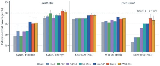
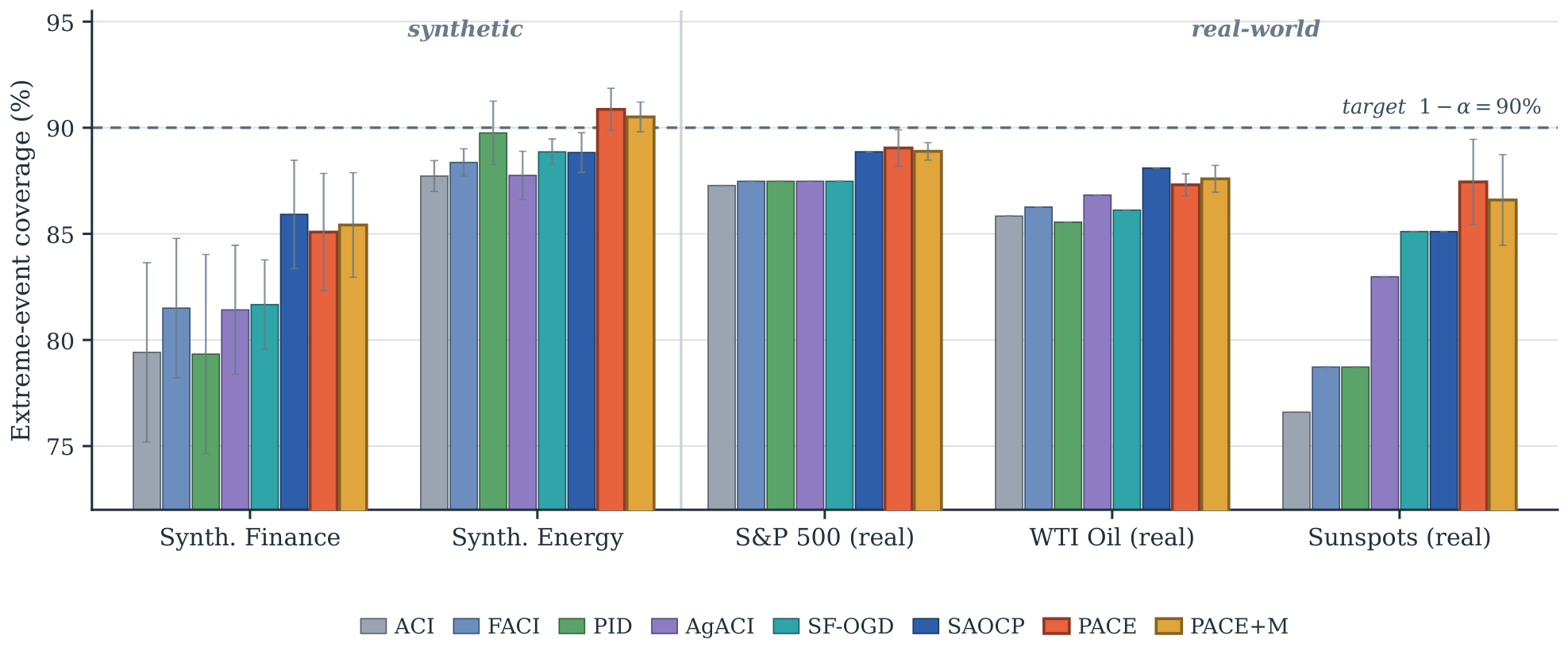
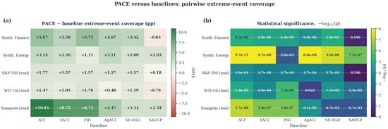
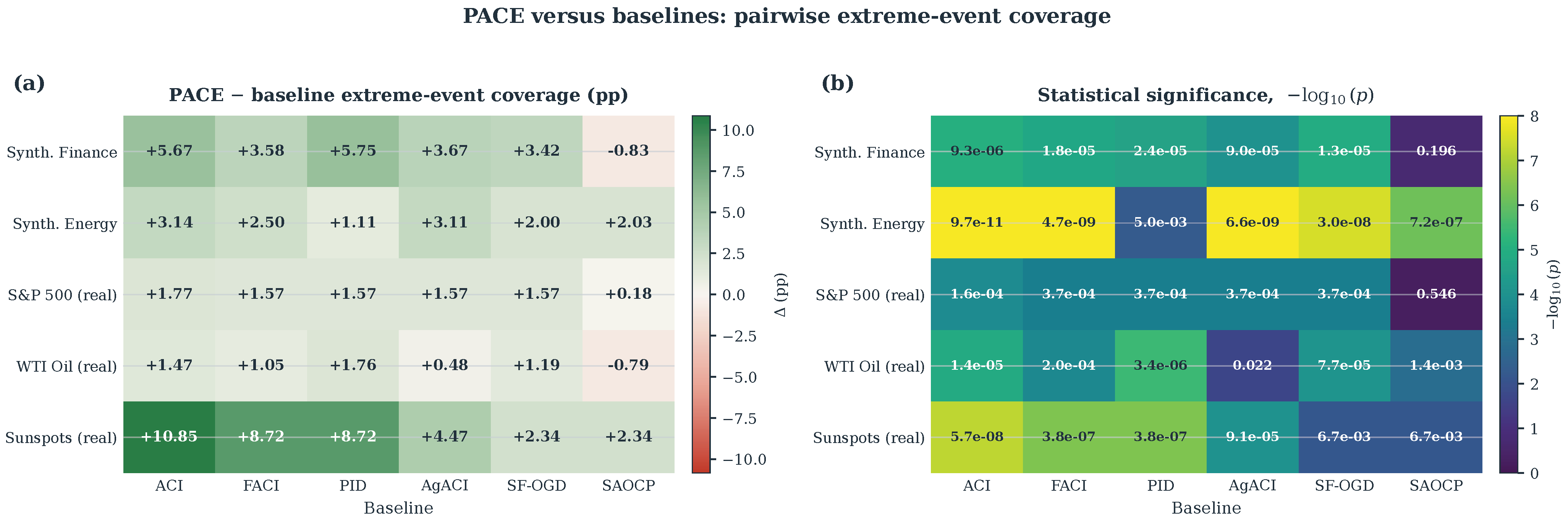
All 25 pairwise comparisons are significant at $p<0.05$, and 22 remain significant at $p<0.001$. The three exceptions to the latter threshold are PACE versus PID on synthetic energy ($p=0.005$), AgACI on WTI ($p=0.022$), and SF-OGD on sunspots ($p=0.007$). Figure 1 summarizes the comparison across datasets and methods, while Figure 2 presents the corresponding significance grid. These results show that PACE’s extreme-regime coverage advantage over single-calibrator adaptive methods is consistent across synthetic and real data and across both short and long regime structures. This pattern also holds against the strongest single-calibrator baselines, PID-Conformal and SF-OGD. Section 4.6 reports the interval-score results, which are less favorable to PACE and provide an important counterpoint to the coverage comparison.

Figure 1. Extreme-event coverage across methods and datasets. Error bars show the standard deviation across seeds; they are zero for deterministic baselines on the real datasets. The dotted line indicates the target $1-\alpha =0.90$. PACE achieves higher coverage than all five non-SAOCP baselines on every dataset. PACE and SAOCP remain competitive throughout, with PACE leading on three datasets and SAOCP on two.

Figure 2. Pairwise significance results for PACE against each comparator. (a) Difference in coverage, in percentage points, computed as PACE minus the baseline. (b) Statistical significance shown as $-{\log }_{10}\left(p\right)$. The only cells in which PACE does not have significantly higher coverage are the two datasets where SAOCP attains higher extreme-regime coverage—synthetic finance (not significant) and WTI ($p=0.001$)—and the near-tie on S&P 500 ($p=0.55$). The reported p-values are not adjusted for multiple comparisons; see Section 4.1.

4.3. PACE Versus SAOCP: The Central Comparison

Table 2 gives the head-to-head results. The two synthetic datasets are especially useful because their regime structures are known by construction. Synthetic Finance contains crashes lasting $\{15,20,25\}$ steps, all short relative to PACE’s median window of approximately 80, and SAOCP obtains higher coverage in this setting. Synthetic Energy contains heatwaves and cold snaps lasting $\{72,96,120\}$ steps, which are long relative to the median window, and PACE leads by $2.0$ pp. The real datasets do not divide as neatly according to mean event duration. WTI has the longest mean duration among them ($19.1$ steps) but favors SAOCP, whereas sunspots has a shorter mean duration ($11.8$ steps) and favors PACE. The reason is that a dataset-level mean can conceal a heavy-tailed mixture of short and long events. For example, one multi-month oil crisis raises WTI’s mean even though most WTI extreme regimes are brief. We therefore move from dataset averages to an event-level analysis.

Table 2. Head-to-head comparison of PACE and SAOCP on extreme-event coverage in the main experiment suite. Significance is assessed with a paired t-test on the synthetic datasets, where SAOCP is run with 20 seeds, and a one-sample t-test on the real datasets, where SAOCP is deterministic. Independent robustness reruns in Section 5 use new random seeds and data-generation draws and are reported separately.

Dataset	PACE (%)	SAOCP (%)	$\mathbf{\Delta }$ (pp)	p	Winner
Synthetic Finance	$85.08\pm 2.76$	$85.92\pm 2.55$	$-0.83$	$0.196$	SAOCP (n.s.)
Synthetic Energy	$90.86\pm 0.99$	$88.83\pm 0.93$	$+2.03$	<${10}^{-6}$	PACE
S&P 500	$89.05\pm 0.85$	$88.87$ (det.)	$+0.18$	$0.546$	tie (n.s.)
WTI Crude Oil	$87.31\pm 0.52$	$88.10$ (det.)	$-0.79$	$0.001$	SAOCP
Sunspots	$87.45\pm 2.01$	$85.11$ (det.)	$+2.34$	$0.007$	PACE

4.4. The Duration Heuristic

The dataset-level results point to event duration as a possible factor separating PACE from SAOCP. The methodological discussion in Section 3.4 leads to the same prediction. SAOCP creates and warms up a new expert after each regime change, incurring a delay related to that expert’s lifetime. PACE, by contrast, already has short-window members running when the change occurs, but it needs observations from the new event to accumulate fitness on the appropriate members. These mechanisms suggest an advantage for SAOCP during short extreme events and for PACE during longer ones. We test this hypothesis at the level of individual events.

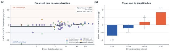
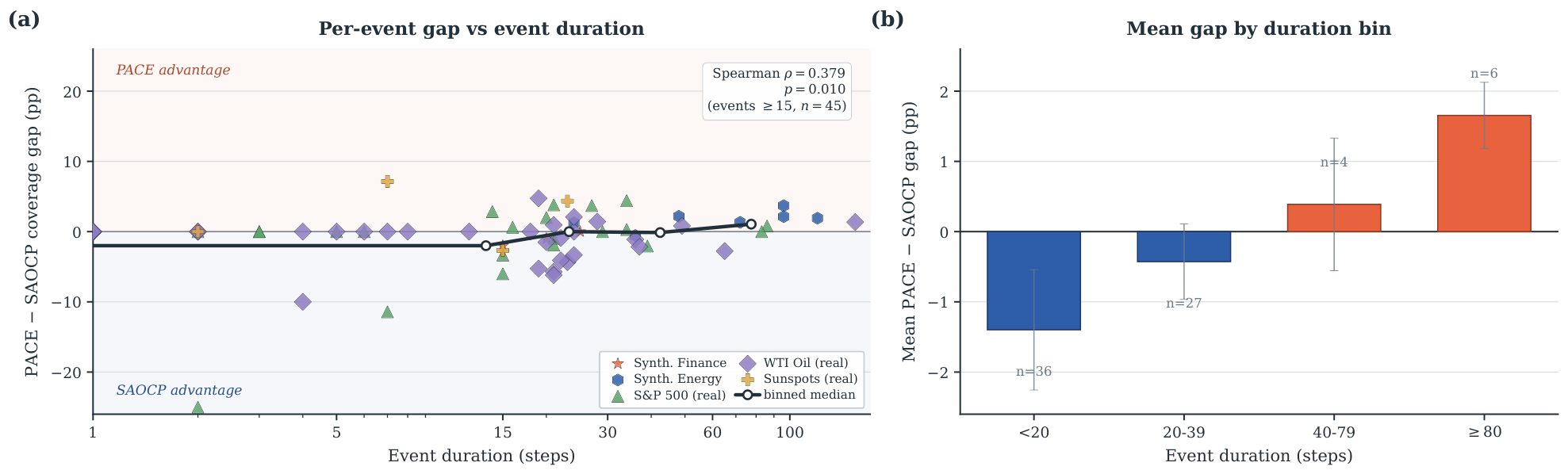
We pool the 73 extreme regimes from all five datasets and, for each regime, compute mean PACE coverage minus mean SAOCP coverage. Figure 3a plots this difference against event duration on a logarithmic duration axis. The pattern is noisy for short events, where coverage is estimated from only a few observations, but it becomes clearer as event duration increases. We quantify the association using Spearman rank correlation between event duration and the PACE–SAOCP coverage gap. Across all 73 events, the correlation is $\rho =0.231$ ($p=0.049$). Restricting the analysis to events lasting at least 15 steps, for which per-event coverage is more stable, increases the correlation to $\rho =0.379$. Pearson correlation has the same sign but somewhat larger p-values. We therefore emphasize the rank correlation, which is better suited to the heavy-tailed duration distribution. Figure 3b and Table 3 report the mean coverage difference within four duration bins. The bin averages increase monotonically with duration.

Figure 3. Event duration as an empirical heuristic. (a) Per-regime difference between PACE and SAOCP coverage, plotted against event duration for all five datasets ($n=73$). Marker shape identifies the dataset, as shown in the inset legend, and the dashed gray curve gives a five-bin mean trend. (b) Mean coverage difference within duration bins, with error bars showing $\pm 1$ SE. The mean favors SAOCP for events shorter than 40 steps and PACE for longer events. Spearman correlation between duration and the coverage difference is $\rho =0.379$, $p=0.010$ for events lasting at least 15 steps ($n=45$), and $\rho =0.231$, $p=0.049$ for the full set of 73 events.

Table 3. Mean per-event difference between PACE and SAOCP extreme-event coverage within four event-duration bins, pooled over the 73 extreme regimes identified across the five datasets. Positive values favor PACE.

Event Duration (Steps)	Mean PACE–SAOCP Gap (pp)
<20 ($n=36$)	$-1.40$
$[20,40)$ ($n=27$)	$-0.43$
$[40,80)$ ($n=4$)	$+0.39$
≥80 ($n=6$)	$+1.65$

The sign of the bin average changes from negative, indicating a SAOCP advantage for shorter events, to positive, indicating a PACE advantage for longer events. Two qualifications are important. First, the correlation in the full event pool is only borderline significant ($\rho =0.231$, $p=0.049$, $n=73$). Restricting attention to events of at least 15 steps strengthens the association to $\rho =0.379$ ($p=0.010$), but removes 28 short events. Second, the two longest-duration bins contain few events ($n=4$ for $[40,80)$ and $n=6$ for ≥80), so their positive means are estimated imprecisely. In this event pool, the average difference changes sign in the $[20,40)$ bin. That location should be interpreted as the center of a noisy transition. The more robust conclusion is that the population-of-rules and population-of-intervals strategies capture complementary forms of temporal structure, and their relative performance depends on the duration of an extreme event compared with the score window.

4.5. Adaptation Dynamics

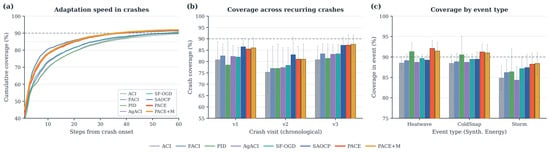
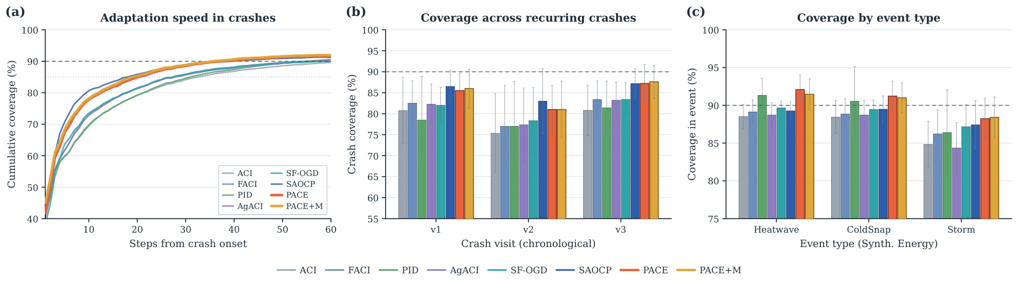
Figure 4a tracks cumulative coverage from the start of an extreme event, averaged over events and seeds in the synthetic-finance benchmark. ACI and PID require approximately 30 steps to reach $85\%$ coverage after event onset. FACI, AgACI, and SF-OGD reach that level after roughly 15 to 18 steps, whereas SAOCP and PACE do so within about 7 to 10 steps. The curves for PACE and SAOCP are nearly indistinguishable. Figure 4b,c report crash coverage by visit number and coverage by event type, respectively.

Figure 4. Adaptation dynamics on the synthetic datasets. (a) Cumulative coverage after event onset, averaged over events and 20 seeds on synthetic finance. (b) Crash coverage by visit number: v1, v2, and v3 refer to the first, second, and third crash regimes encountered chronologically in the synthetic-finance series. The panel therefore indicates whether coverage on a recurring crash type changes across later visits. (c) Coverage by event type on synthetic energy. In panel (a), PACE and SAOCP follow almost identical trajectories and both adapt visibly faster than the five non-SAOCP baselines. In every panel the dashed horizontal line marks the target coverage $1-\alpha =0.90$; the dotted line in panel (a) marks the $85\%$ level referred to in the text. Error bars show $\pm 1$ standard deviation across seeds.

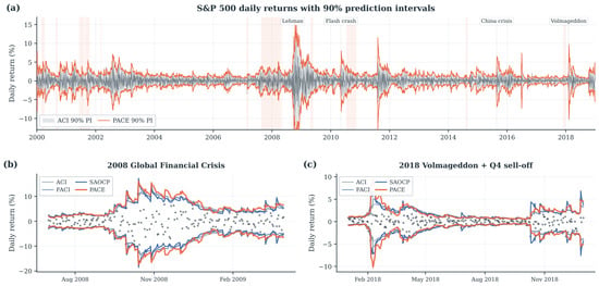
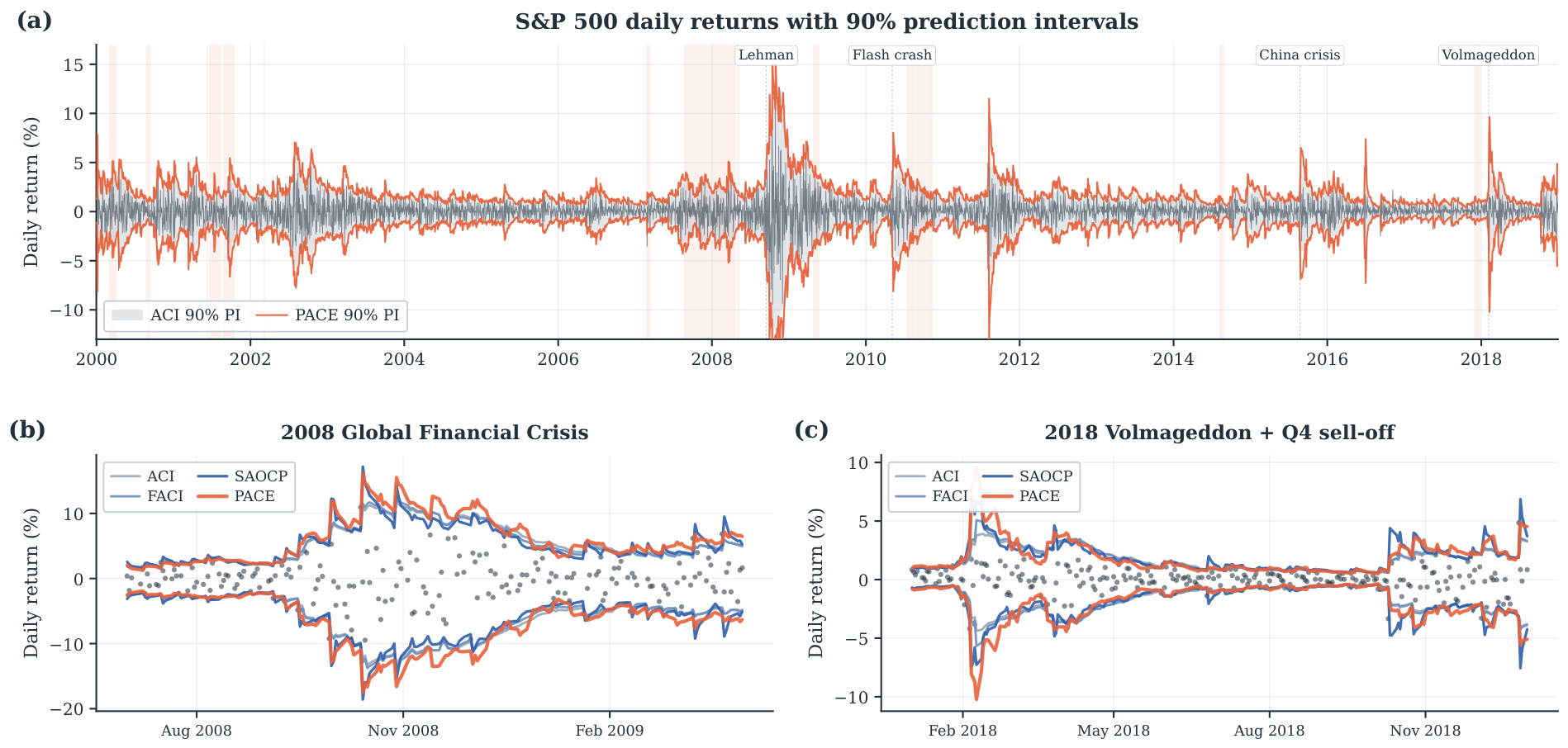
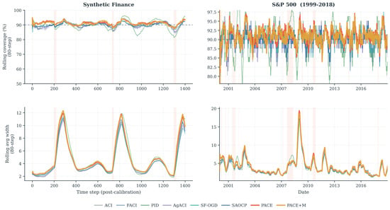
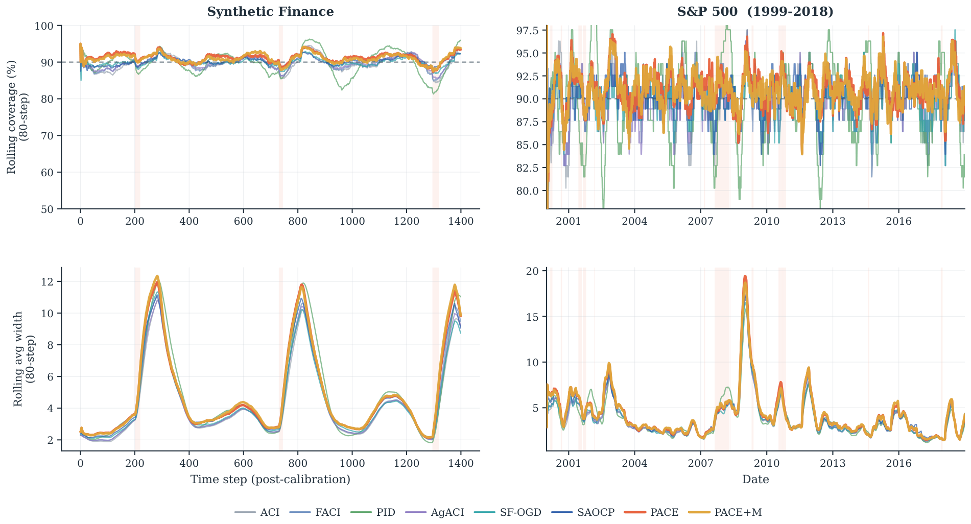
Figure 5 displays representative prediction intervals over the full 20-year S&P 500 evaluation period, with detailed views of the 2008 Global Financial Crisis and the 2018 “Volmageddon”. ACI widens too slowly during the GFC, whereas PACE and SAOCP both expand their intervals rapidly around the crash and contract them during the subsequent recovery. Figure 6 shows rolling coverage and rolling interval width over the complete S&P 500 series. PACE/PACE+M and SAOCP follow similar trajectories and generally maintain higher rolling coverage than the five non-SAOCP baselines.

Figure 5. Prediction intervals for the S&P 500. (a) The full 2000–2018 evaluation window, in which the red shading marks the retrospectively identified extreme regimes defined in Section 4.1. (b) The 2008 Global Financial Crisis, during which ACI and FACI under-cover for several months while PACE and SAOCP widen quickly and recover. (c) The 2018 “Volmageddon” volatility spike and fourth-quarter sell-off. In panels (b,c) the dots are the realized daily log-returns and the bands are the corresponding prediction intervals.

Figure 6. Rolling coverage and rolling interval width over the full evaluation periods for synthetic finance (left; mean over 20 seeds) and the S&P 500 (right). PACE and SAOCP generally remain above the five non-SAOCP baselines in rolling coverage, while their interval widths rise together during regime changes. Pink shading denotes extreme regimes.

4.6. Width-Coverage Trade-Off

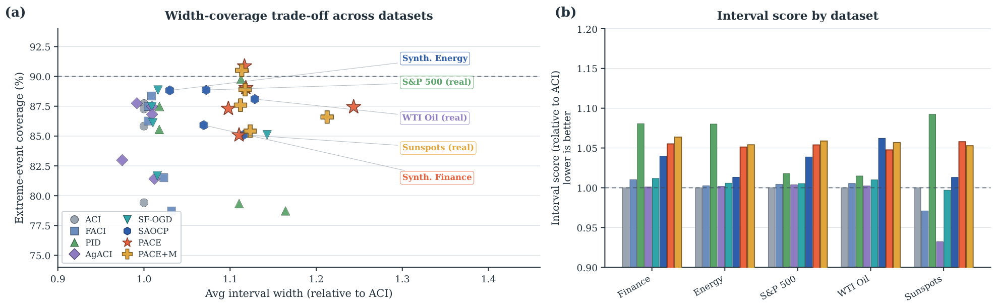
PACE usually obtains its coverage gains with moderately wider intervals, although the result is not a uniform width penalty. The ratio of PACE width to SAOCP width is $1.038$ on synthetic finance, $1.084$ on synthetic energy, $1.043$ on S&P 500, $0.973$ on WTI, where PACE is slightly narrower, and $1.114$ on sunspots. Thus, the relative width difference ranges from $-2.7\%$ to $+11.4\%$. The interval score jointly penalizes width and miscoverage and ranks SAOCP slightly ahead of PACE on every dataset except WTI, as shown in Figure 7b. On the Pareto frontier defined by extreme-event coverage and interval width, PACE and SAOCP both dominate the five non-SAOCP baselines, but neither dominates the other.

Figure 7. Trade-off between interval width and extreme-event coverage. (a) Extreme-event coverage plotted against average interval width relative to ACI, with one point per method and dataset. PACE (star) and SAOCP (hexagon) jointly dominate the simpler baselines in coverage. (b) Interval score, where lower values are better, relative to ACI for each dataset. SAOCP achieves a slightly better interval score than PACE on every dataset except WTI. The dashed reference line marks the target coverage $1-\alpha =0.90$ in panel (a) and the ACI baseline level of $1.00$ in panel (b).

4.7. Mechanism Ablations

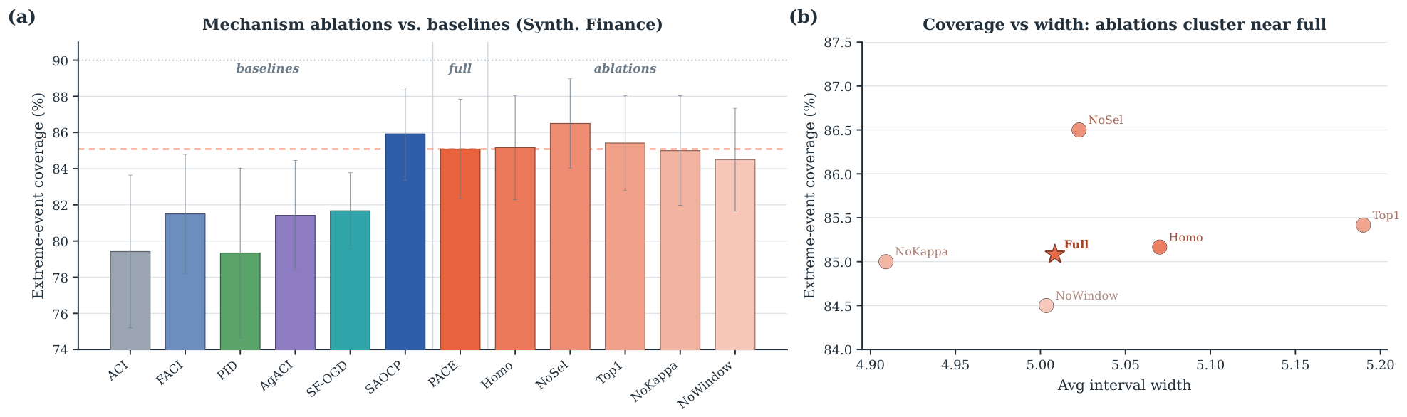
We examine five PACE ablations on the synthetic-finance benchmark (Figure 8):

Figure 8. Ablations of PACE mechanisms on synthetic finance. (a) Extreme-event coverage for the five non-SAOCP baselines, SAOCP, full PACE, and the five ablation variants. Every ablation lies within one standard deviation of full PACE. (b) Coverage plotted against interval width; the ablations cluster closely around full PACE. In panel (a), the dotted line marks the target coverage $1-\alpha =0.90$ and the dashed line marks the level attained by full PACE; error bars show $\pm 1$ standard deviation across seeds. In panel (b), the star marks full PACE and the circles mark the ablation variants, each labeled with its variant name.

• PACE-Homo: every member is initialized with the same parameters, $w=50$, $\lambda =0.95$, and $\kappa =1.0$;
• PACE-NoSel: clonal selection is disabled, leaving the randomly initialized population fixed;
• PACE-Top1: the prediction uses only the highest-fitness member rather than the top-K members;
• PACE-NoKappa: $\kappa$ is fixed at $1.0$;
• PACE-NoWindow: the window-length and decay-rate ranges are each reduced to a single value.

The ablations produce a notably tight cluster of results. Every variant remains within one standard deviation of full PACE, with extreme-event coverage between $85.0\%$ and $86.5\%$, compared with $85.1\%$ for full PACE (Table 4):

Table 4. Extreme-event coverage of the five PACE ablation variants on the synthetic-finance benchmark, in percent (mean ± standard deviation across 20 seeds; target $1-\alpha =90$%).

Variant	Extreme cov. (%)
PACE-Full	$85.08\pm 2.76$
PACE-Homo	$85.17\pm 2.88$
PACE-NoSel	$86.50\pm 2.47$
PACE-Top1	$85.42\pm 2.63$
PACE-NoKappa	$85.00\pm 3.03$
PACE-NoWindow	$84.50\pm 2.84$

These results do not identify any single mechanism as indispensable, but the PACE-Homo result requires care. PACE-Homo gives every member the same initial $(w,\lambda ,\kappa )$ values, yet it leaves clonal selection active. The members therefore begin identically but diverge as the periodic mutation step in Algorithm 1 replaces the lowest-fitness third with perturbed copies of the strongest members. After several hundred steps, the population is no longer homogeneous because selection has generated diversity. The fact that PACE-Homo matches full PACE therefore does not show that heterogeneity is unnecessary. Instead, it shows that the required heterogeneity can be created during learning. PACE-NoWindow is the closest approximation to a persistently homogeneous population because it fixes both window length and decay rate, and it shows the largest coverage reduction ($-0.58$ pp). Disabling clonal selection in PACE-NoSel raises coverage by $+1.42$ pp on this benchmark. We interpret this as evidence that the initial random diversity is already sufficient for this task, while selection adds variance without a corresponding gain in signal.

We therefore do not claim that any individual design choice is necessary by itself. The broader structural feature appears to be the aggregation of multiple quantile calibrators together with some source of heterogeneity, whether introduced at initialization, generated through selection, or supplied by both. SAOCP supports this interpretation: its ensemble has a different structure, based on per-step spawning over dyadic intervals, yet it achieves comparable extreme-regime coverage. We accordingly view ensemble aggregation of online quantile calibrators as a general design space in which PACE and SAOCP are two distinct constructions. PACE’s heterogeneous-horizon population is a natural member of this class, but the present evidence does not establish it as the only effective one. We repeat the ablation on synthetic energy in Section 5.4. The cross-dataset results identify different leading mechanisms: window and decay-rate diversity have the largest effect on synthetic finance, whereas quantile-scale diversity has the largest effect on synthetic energy. Removing clonal selection or top-K aggregation changes coverage by less than one seed standard deviation on both datasets. The relative importance of the mechanisms is therefore dataset-dependent.

4.8. The PACE+M Memory Bank: A Null Finding

An earlier version of PACE used an optional memory bank that stored high-fitness score functions and recalled them when the regime detector identified a familiar volatility level. The intended benefit was faster adaptation to short, recurring events. The experiments do not support this hypothesis. Across the five datasets, the difference in extreme-event coverage between PACE+M and PACE ranges from $-0.85$ pp on sunspots to $+0.34$ pp on synthetic finance, and none of the comparisons is significant at $p<0.05$. We retain PACE+M in Table 1 for transparency, but treat the result as a null finding. A likely difficulty is that each memory entry must be tagged with a regime descriptor that is informative enough to support useful recall while still being computable without access to ground-truth regime labels.

5. Robustness Experiments

We examine whether the paper’s conclusions are robust to several design and evaluation choices: the target level $\alpha$, the population size N, the dataset used for the ablation study, the distinction between plain ensembling and PACE’s specific mechanisms, event duration under a controlled design, and financial risk backtesting. The robustness experiments use a self-contained re-implementation of PACE and the adaptive baselines described in Section 3. Because they rely on independent random seeds and data-generation draws, their absolute coverage values are not expected to reproduce those in the main experiment tables. We therefore interpret them as checks of the qualitative findings.

5.1. Sensitivity to the Target Level $\alpha$

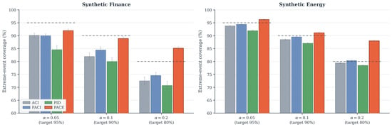
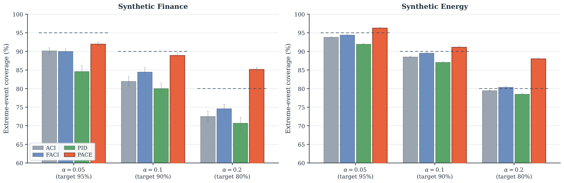
The experiments use $\alpha =0.10$. To assess whether the findings depend on this choice, Figure 9 repeats the comparison with ACI, FACI, and PID at $\alpha \in \{0.05,0.10,0.20\}$ on both synthetic datasets. PACE achieves the highest extreme-event coverage among the four methods at every target level on both datasets. On synthetic finance, its extreme-event coverage is $91.9\%$, $88.9\%$, and $85.1\%$ for $\alpha =0.05,0.10,0.20$, respectively, compared with targets of $95\%$, $90\%$, and $80\%$. The strongest baseline, either FACI or ACI, reaches only $90.0\%$, $84.4\%$, and $74.6\%$. The separation between PACE and the baselines becomes larger as $\alpha$ increases. This pattern is plausible because larger values of $\alpha$ produce narrower intervals, leaving a single tracker less room to absorb an abrupt regime change and increasing the value of pooling trackers. Since the ordering of the methods remains unchanged across all three values of $\alpha$, the main conclusion does not appear to be an artifact of selecting a $90\%$ target.

Figure 9. Extreme-event coverage at target levels $\alpha \in \{0.05,0.10,0.20\}$ on the two synthetic datasets. Dotted lines indicate the corresponding $1-\alpha$ targets. PACE has the highest coverage among the four methods at every level, with a larger advantage at higher values of $\alpha$.

5.2. Sensitivity to the Population Size N

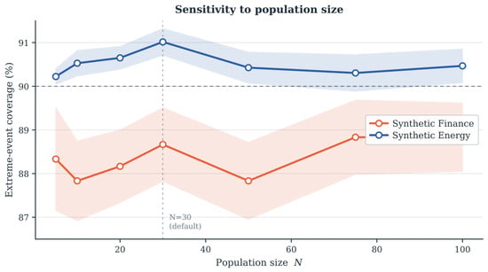
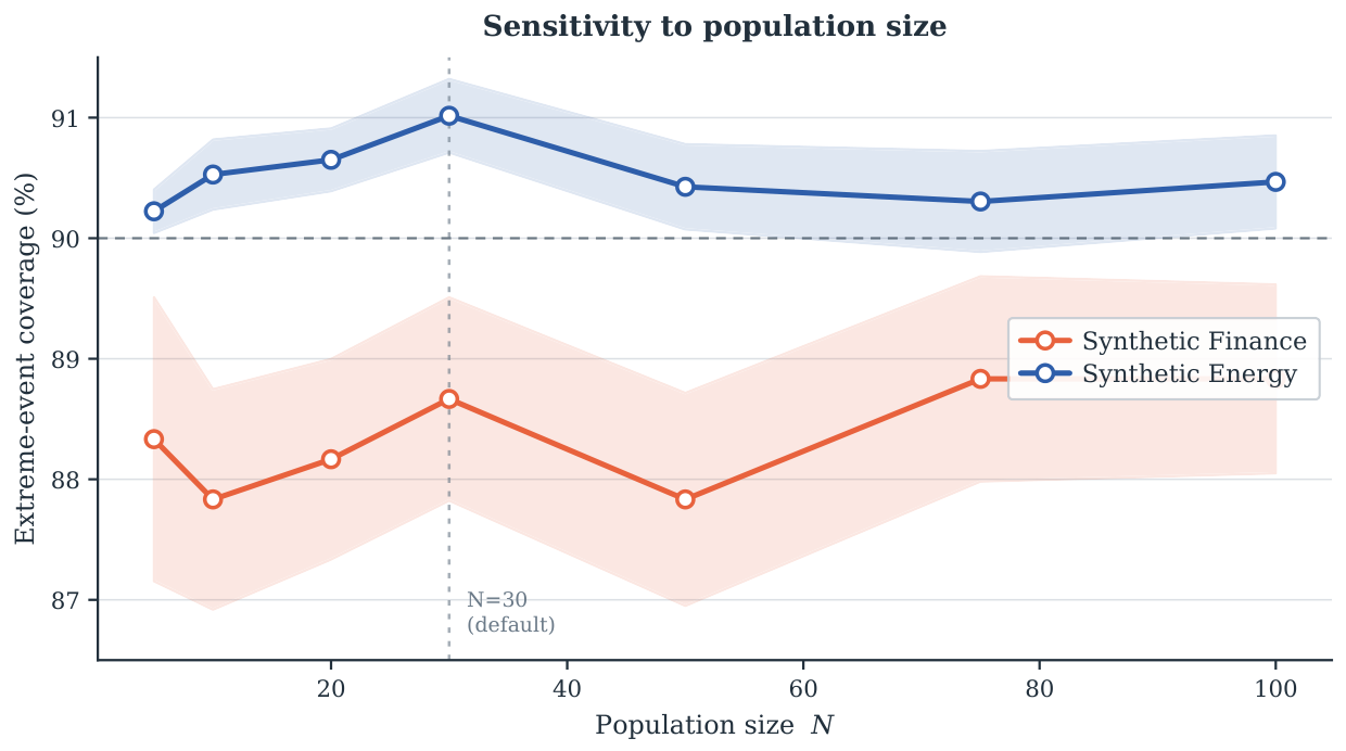
Figure 10 evaluates population sizes from $N=5$ to $N=100$. Extreme-event coverage changes very little over this range. On synthetic finance, it remains within approximately one percentage point of the value obtained with $N=30$, increasing from $88.3\%$ at $N=5$ to $88.8\%$ at $N=100$. On synthetic energy, the variation is also less than one percentage point, from $90.2\%$ at $N=5$ to $90.5\%$ at $N=100$. Performance largely saturates by $N\approx 20$, and even a population of only five members retains nearly all of the improvement. This insensitivity suggests that the gains do not arise from a large ensemble simply averaging away variance. Instead, they appear to come from maintaining a small set of trackers that operate at meaningfully different time scales. The result also indicates that the population can be reduced substantially when computational cost is a concern.

Figure 10. Extreme-event coverage as a function of population size N (mean ± 1 SE over 10 seeds). Coverage largely saturates by $N\approx 20$ and changes little thereafter; even $N=5$ retains most of the improvement. The horizontal dashed line marks the target coverage $1-\alpha =0.90$ and the vertical dashed line marks the default population size $N=30$.

5.3. Ensembling Versus PACE’s Mechanisms

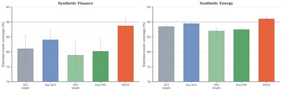
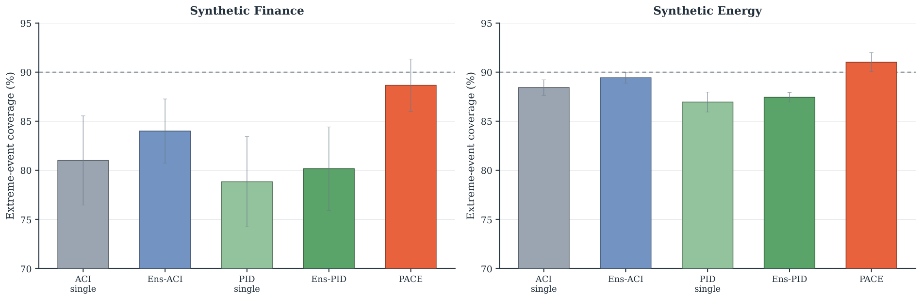
One possible explanation for PACE’s advantage is that it combines several trackers. To separate this general ensemble effect from the contribution of PACE’s selection and aggregation rules, we construct plain ensembles of ACI and PID. Each ensemble averages five instances with window sizes $\{20,50,80,120,150\}$ and uses no fitness weighting, selection, or quantile-scale diversity. Figure 11 compares these ensembles with their single-tracker counterparts and with PACE. Plain ensembling is beneficial: relative to a single ACI tracker, Ensemble-ACI increases extreme-event coverage by approximately $3.0$ pp on synthetic finance and $1.0$ pp on synthetic energy. PACE nevertheless improves further, reaching $88.7\%$ and $91.0\%$, compared with $84.0\%$ and $89.4\%$ for Ensemble-ACI. Thus, ordinary ensembling accounts for part of the gain, but not all of it. The additional improvement is associated with PACE’s heterogeneous windows and decay rates, quantile-scale diversity, and fitness-weighted top-K aggregation.

Figure 11. Plain ACI and PID ensembles, formed by averaging five window sizes, compared with the corresponding single-tracker methods and with PACE. Ensembling improves coverage, but PACE provides a further gain, indicating that its specific mechanisms contribute beyond averaging alone. The dashed horizontal line marks the target coverage $1-\alpha =0.90$ and the error bars show $\pm 1$ standard deviation across seeds.

5.4. Cross-Dataset Ablation

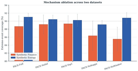
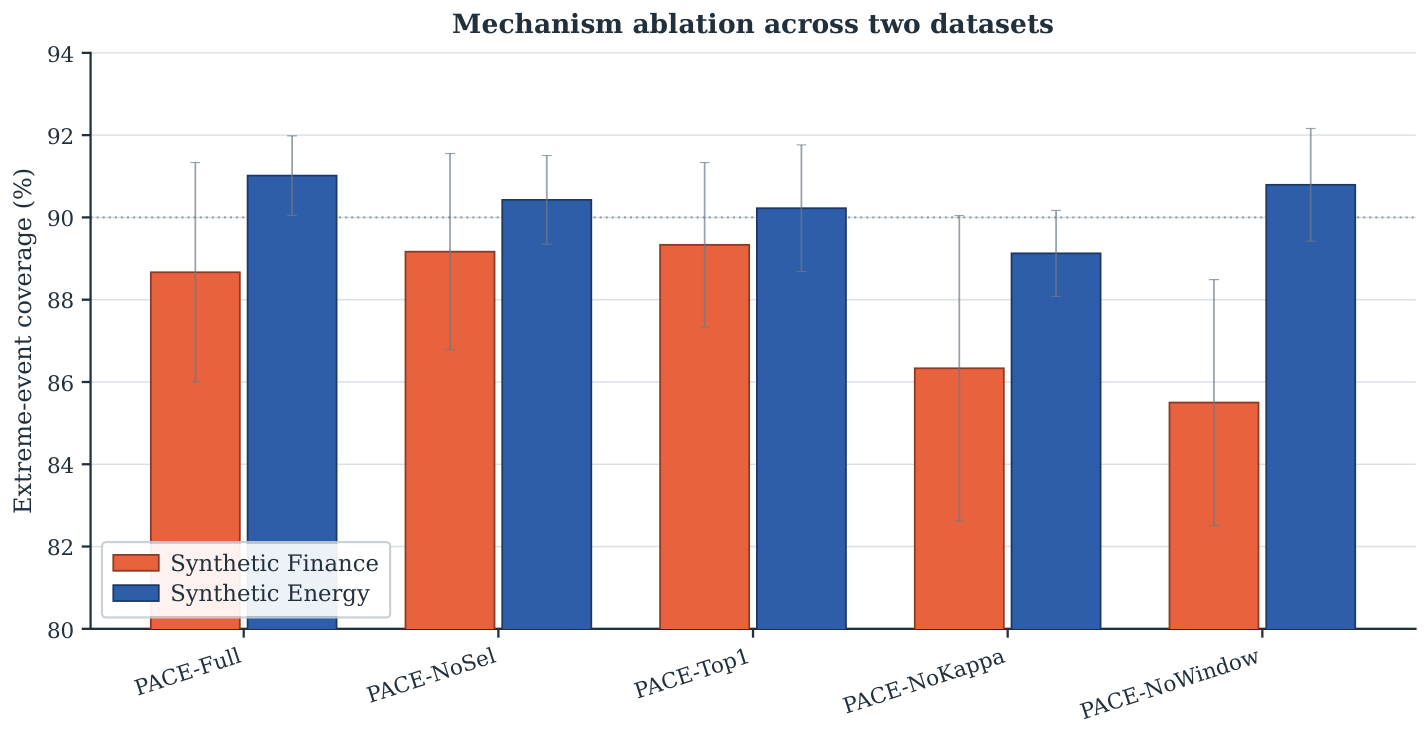
The mechanism ablation in Section 4.7 was conducted only on synthetic finance. Figure 12 repeats the analysis on synthetic energy to determine whether the same conclusions hold in a different setting. The most influential mechanism is dataset-dependent. On synthetic finance, removing window and decay-rate diversity in PACE-NoWindow produces the largest reduction in coverage, $-3.2$ pp, while PACE-NoKappa reduces coverage by $-2.3$ pp. On synthetic energy, removing quantile-scale diversity in PACE-NoKappa produces the largest reduction, $-1.9$ pp, whereas PACE-NoWindow has little effect. On both datasets, removing clonal selection or top-K aggregation changes coverage by less than the standard deviation across seeds. Thus, the two benchmarks support the broader importance of heterogeneous calibration, but they do not identify one universally dominant component.

Figure 12. Mechanism ablation on two datasets (mean ± 1 SD over 10 seeds). The leading mechanism is dataset-dependent: window and decay-rate diversity, removed in PACE-NoWindow, has the largest effect on synthetic finance, whereas quantile-scale diversity, removed in PACE-NoKappa, has the largest effect on synthetic energy. The dotted horizontal line marks the target coverage $1-\alpha =0.90$.

5.5. A Controlled Duration Sweep

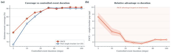
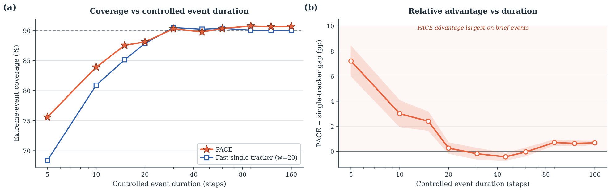
The duration analysis in Section 4.4 combines naturally occurring events of different lengths, so duration may be confounded with other event characteristics. To study duration in isolation, we generate a controlled synthetic series in which every extreme event has the same length D and vary D from 5 to 160 time steps. In this version, the controlled sweep compares PACE with a fast-adapting single tracker, implemented as an ACI instance with a window of 20 rather than with SAOCP. Because this comparator is not SAOCP, we use the experiment only to illustrate how PACE behaves across event durations; it does not validate the PACE-versus-SAOCP comparison. A controlled sweep in which both PACE and SAOCP are evaluated on identical streams remains the appropriate next experiment and is included among the limitations.

Figure 13 reveals a more nuanced pattern than a simple monotonic crossover. PACE’s advantage over the fast single tracker is greatest for very brief events, reaching $+7.2$ pp at $D=5$. The difference then decreases to approximately zero for $D=20$ to 45, before becoming modestly positive again for long events, at $+0.7$ pp for $D\ge 90$. A short-window tracker has too few observations to estimate an in-event quantile reliably when an event lasts only a handful of steps, whereas PACE can pool information across its population. Once the event persists long enough for the single tracker to recalibrate, the two methods perform similarly. The experiment therefore supports the view that PACE’s relative performance depends on event duration, but it also shows that the direction of the effect depends on the comparator. PACE is strongest on short events relative to a naive fast tracker. The opposite ordering observed in Section 4.4 is specific to the comparison with SAOCP, which is designed to respond to brief events by spawning fresh experts.

Figure 13. Controlled duration sweep in which every extreme event has a fixed length D. Panel (a) shows the extreme-event coverage of PACE and a fast single tracker with window 20; panel (b) shows their difference. PACE has its largest advantage on very brief events, and the gap narrows as events become longer. The dashed horizontal line in panel (a) marks the target coverage $1-\alpha =0.90$. In panel (b) the solid horizontal line at zero marks parity between the two methods and the shaded band shows $\pm 1$ standard error across 10 seeds.

5.6. Exploratory Financial Risk Diagnostic

For the financial series, coverage alone is not sufficient to determine whether a method is useful for risk management. As an exploratory diagnostic, we examine breaches of the lower endpoint of each interval on the S&P 500 return series. Because the intervals are symmetric, two-sided $90\%$ prediction intervals calibrated with absolute residuals, the lower endpoint is not a formally calibrated $10\%$ one-sided Value-at-Risk (VaR) estimate. We therefore compare breach frequencies with a $10\%$ reference rate and report the Kupiec proportion-of-failures and Christoffersen independence statistics only as descriptive diagnostics, not as formal VaR validation. Against this reference rate, ACI yields a breach rate of $10.8\%$ with a Kupiec p-value of $0.06$, whereas PACE yields a lower breach rate of $6.8\%$ with a Kupiec p-value below $0.01$. The Christoffersen test finds no significant serial dependence in the breaches of either method, with $p=0.44$ for ACI and $p=0.14$ for PACE. The lower breach frequency for PACE is consistent with its wider, more conservative intervals. A formal VaR backtest would require a one-sided tail-calibrated construction and is left for future work.

6. Discussion and Open Questions

Our experiments support three main conclusions. First, ensemble calibration is effective. Both SAOCP’s dyadic experts and PACE’s heterogeneous-horizon population achieve strong extreme-regime coverage, and neither method dominates across all datasets. The ablation results also suggest that PACE benefits from maintaining several calibration horizons. Second, the practical choice between PACE and SAOCP depends on the coverage–sharpness trade-off. PACE intervals are slightly narrower on WTI but about eleven percent wider on sunspots, and SAOCP has the better interval score on every dataset except WTI. Against the earlier baselines, however, PACE generally improves the coverage width frontier rather than gaining coverage only through wider intervals. PACE is therefore more suitable when avoiding undercoverage is the main priority, whereas SAOCP is preferable when sharper intervals matter more. Third, PACE appears to improve relative to SAOCP as event duration increases, but this pattern is exploratory because the transition is noisy and the evidence for long events is limited.

The main open question is that PACE has no long-run coverage guarantee, and analyses developed for single calibrators do not extend because its final quantile is a non-linear aggregate of members that need not be individually calibrated to the target. The outer multiplicative correction appears to pull rolling coverage back toward the target band, but delayed feedback, unbounded heavy-tailed scores, discontinuous top-K changes, and clipping prevent a simple ACI-style argument. We therefore treat this behavior as empirical and view a coverage bound for population-aggregated conformal predictors as the central theoretical problem. Other questions are whether the duration trend can be formalized as a threshold between dyadic and heterogeneous-horizon ensembles, and why the optional memory bank did not help. A likely difficulty is defining informative regime labels without access to ground-truth states.

Limitations

We evaluate five datasets at target coverage $0.90$. The robustness checks in Section 5 vary $\alpha \in \{0.05,0.10,0.20\}$, the population size N, and the ablation dataset without changing the main conclusions; alternative normalization schemes and multivariate prediction regions remain untested. The real-data baselines are deterministic, and the one-sample t-tests against PACE capture sensitivity to initialization. Block- or event-level resampling with multiplicity correction would provide stronger inference. The controlled duration sweep in Section 5.5 uses a fast single tracker rather than SAOCP. Finally, the 73-event analysis is dominated by synthetic-energy events, and the longest-duration bins contain limited observations.

7. Conclusions

We introduced PACE, a heuristic multi-horizon ensemble of online conformal quantile calibrators for prediction under distribution shift. Across two synthetic and three real-world datasets, PACE attains higher empirical extreme-regime coverage than five adaptive conformal baselines, and relative to SAOCP, it trades interval sharpness for coverage. The most confident contribution is the metric-explicit comparison of when each method is preferable, together with the finding that two very different ensemble structures reach comparable coverage on the same problem, which points to the aggregation of online quantile calibrators as a general and effective design space. PACE does not yet carry a strongly adaptive or long-run coverage guarantee, and its event-duration behavior and outer coverage correction warrant controlled study against SAOCP; establishing a coverage bound for population-aggregated conformal predictors is the most valuable direction this work opens.

References

- Vovk, V.; Gammerman, A.; Shafer, G. Algorithmic Learning in a Random World; Springer: New York, NY, USA, 2005. [Google Scholar]
- Shafer, G.; Vovk, V. A tutorial on conformal prediction. J. Mach. Learn. Res. 2008, 9, 371–421. [Google Scholar]
- Gibbs, I.; Candès, E. Adaptive conformal inference under distribution shift. In Proceedings of the Advances in Neural Information Processing Systems; Curran Associates, Inc.: Red Hook, NY, USA, 2021; Volume 34, pp. 1660–1672. [Google Scholar]
- Gibbs, I.; Candès, E. Conformal inference for online prediction with arbitrary distribution shifts. J. Mach. Learn. Res. 2024, 25, 1–36. [Google Scholar]
- Bhatnagar, A.; Wang, H.; Xiong, C.; Bai, Y. Improved online conformal prediction via strongly adaptive online learning. In Proceedings of the 40th International Conference on Machine Learning, Honolulu, HI, USA, 23–29 July 2023; PMLR: Cambridge, MA, USA, 2023; Volume 202, pp. 2337–2363. [Google Scholar]
- Lei, J.; G’Sell, M.; Rinaldo, A.; Tibshirani, R.J.; Wasserman, L. Distribution-free predictive inference for regression. J. Am. Stat. Assoc. 2018, 113, 1094–1111. [Google Scholar] [CrossRef] [Scilit]
- Romano, Y.; Patterson, E.; Candès, E.J. Conformalized quantile regression. In Proceedings of the Advances in Neural Information Processing Systems; Curran Associates, Inc.: Red Hook, NY, USA, 2019; Volume 32, pp. 3543–3553. [Google Scholar]
- Angelopoulos, A.N.; Bates, S. Conformal prediction: A gentle introduction. Found. Trends Mach. Learn. 2023, 16, 494–591. [Google Scholar] [CrossRef] [Scilit]
- Barber, R.F.; Candès, E.J.; Ramdas, A.; Tibshirani, R.J. Conformal prediction beyond exchangeability. Ann. Stat. 2023, 51, 816–845. [Google Scholar] [CrossRef] [Scilit]
- Tibshirani, R.J.; Barber, R.F.; Candès, E.J.; Ramdas, A. Conformal prediction under covariate shift. In Proceedings of the Advances in Neural Information Processing Systems; Curran Associates, Inc.: Red Hook, NY, USA, 2019; Volume 32, pp. 2530–2540. [Google Scholar]
- Zaffran, M.; Féron, O.; Goude, Y.; Josse, J.; Dieuleveut, A. Adaptive conformal predictions for time series. In Proceedings of the 39th International Conference on Machine Learning, Baltimore, MD, USA, 17–23 July 2022; PMLR: Cambridge, MA, USA, 2022; Volume 162, pp. 25834–25866. [Google Scholar]
- Angelopoulos, A.N.; Candès, E.J.; Tibshirani, R.J. Conformal PID control for time series prediction. In Proceedings of the Advances in Neural Information Processing Systems; Curran Associates, Inc.: Red Hook, NY, USA, 2023; Volume 36, pp. 23047–23074. [Google Scholar]
- Xu, C.; Xie, Y. Conformal prediction interval for dynamic time-series. In Proceedings of the 38th International Conference on Machine Learning, Virtual, 18–24 July 2021; PMLR: Cambridge, MA, USA, 2021; Volume 139, pp. 11559–11569. [Google Scholar]
- Xu, C.; Xie, Y. Sequential predictive conformal inference for time series. In Proceedings of the 40th International Conference on Machine Learning, Honolulu, HI, USA, 23–29 July 2023; PMLR: Cambridge, MA, USA, 2023; Volume 202, pp. 38707–38727. [Google Scholar]
- Stankeviciute, K.; Alaa, A.M.; van der Schaar, M. Conformal time-series forecasting. In Proceedings of the Advances in Neural Information Processing Systems; Curran Associates, Inc.: Red Hook, NY, USA, 2021; Volume 34, pp. 6216–6228. [Google Scholar]
- Millard, D.; Lindemann, L.; Baheri, A. Split Conformal Prediction in the Function Space with Neural Operators. arXiv 2025, arXiv:2509.04623. [Google Scholar]
- Hamilton, J.D. A new approach to the economic analysis of nonstationary time series and the business cycle. Econometrica 1989, 57, 357–384. [Google Scholar] [CrossRef] [Scilit]
- Aminikhanghahi, S.; Cook, D.J. A survey of methods for time series change point detection. Knowl. Inf. Syst. 2017, 51, 339–367. [Google Scholar] [CrossRef] [Scilit] [PubMed]
- Chernozhukov, V.; Wüthrich, K.; Zhu, Y. Exact and robust conformal inference methods for predictive machine learning with dependent data. In Proceedings of the 31st Conference on Learning Theory, Stockholm, Sweden, 6–9 July 2018; PMLR: Cambridge, MA, USA, 2018; Volume 75, pp. 732–749. [Google Scholar]
- Castro, L.N.; Von Zuben, F.J. Learning and optimization using the clonal selection principle. IEEE Trans. Evol. Comput. 2002, 6, 239–251. [Google Scholar] [CrossRef] [Scilit]
- Castro, L.N.; Timmis, J. Artificial Immune Systems: A New Computational Intelligence Approach; Springer: London, UK, 2002. [Google Scholar]
- Hansen, L.K.; Salamon, P. Neural network ensembles. IEEE Trans. Pattern Anal. Mach. Intell. 1990, 12, 993–1001. [Google Scholar] [CrossRef] [Scilit]
- Krogh, A.; Vedelsby, J. Neural network ensembles, cross validation, and active learning. In Proceedings of the Advances in Neural Information Processing Systems; Curran Associates, Inc.: Red Hook, NY, USA, 1994; Volume 7, pp. 231–238. [Google Scholar]
- Dietterich, T.G. Ensemble methods in machine learning. In Multiple Classifier Systems; Lecture Notes in Computer Science; Springer: Berlin/Heidelberg, Germany, 2000; Volume 1857, pp. 1–15. [Google Scholar]
- Baheri, A.; Amiri Shahbazi, M. Conformal prediction across scales: Finite-sample coverage with hierarchical efficiency. Results Appl. Math. 2025, 26, 100589. [Google Scholar] [CrossRef] [Scilit]
- Amiri Shahbazi, M.; Baheri, A.; Azadeh-Fard, N. A hierarchical conformal framework for uncertainty-aware length of stay prediction in multi-hospital settings. Sci. Rep. 2026, 16, 6564. [Google Scholar] [CrossRef] [Scilit] [PubMed]
- Gneiting, T.; Raftery, A.E. Strictly proper scoring rules, prediction, and estimation. J. Am. Stat. Assoc. 2007, 102, 359–378. [Google Scholar] [CrossRef] [Scilit]
Disclaimer/Publisher’s Note: The statements, opinions and data contained in all publications are solely those of the individual author(s) and contributor(s) and not of MDPI and/or the editor(s). MDPI and/or the editor(s) disclaim responsibility for any injury to people or property resulting from any ideas, methods, instructions or products referred to in the content. |
© 2026 by the authors. Licensee MDPI, Basel, Switzerland. This article is an open access article distributed under the terms and conditions of the Creative Commons Attribution (CC BY) license.