


Abstract
These notes comprise the material I presented during the International Workshop and School on Hadron Structure & Strong Interactions which took place in Nanjing in 2025. The aim of the lectures was to introduce and motivate the study of Generalised Parton Distributions (GPDs) for an audience of Master and Ph.D. students in hadron physics, with little to no background regarding the description of exclusive processes at high virtuality.
1. Foreword
The lectures presented in Nanjing over four hours were intended for an audience with little to no knowledge of exclusive processes, and their description in terms of Generalised Parton Distributions (GPDs) through collinear factorisation. Thus the reader should not expect to find an exhaustive array of technical details here, but rather loose arguments made to allow the students to build their physical intuitions. Some details are nevertheless provided on very specific topics (of personal choices), such as, for instance, the polynomiality property of GPDs. Experienced readers should rather refer to the standard review papers in the field, such as the one by M. Diehl [1] or the one by A. Radyushkin and A. Belitsky [2].
2. Motivation: Probing the Internal Structure of Matter
The aim of this section is to illustrate how scattering experiments allow us to “image” the inner structure of composite objects. Historically, this started with optical diffraction and culminates, for hadrons, in Deeply Virtual Compton Scattering (DVCS), which provides access to GPDs.
2.1. From Fraunhofer Diffraction to Rutherford Scattering
Scattering processes can be used at many different scales in order to map the internal structure of matter. We will start by considering an example that is familiar to all students, the one of Fraunhofer diffraction in optics.
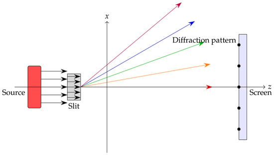
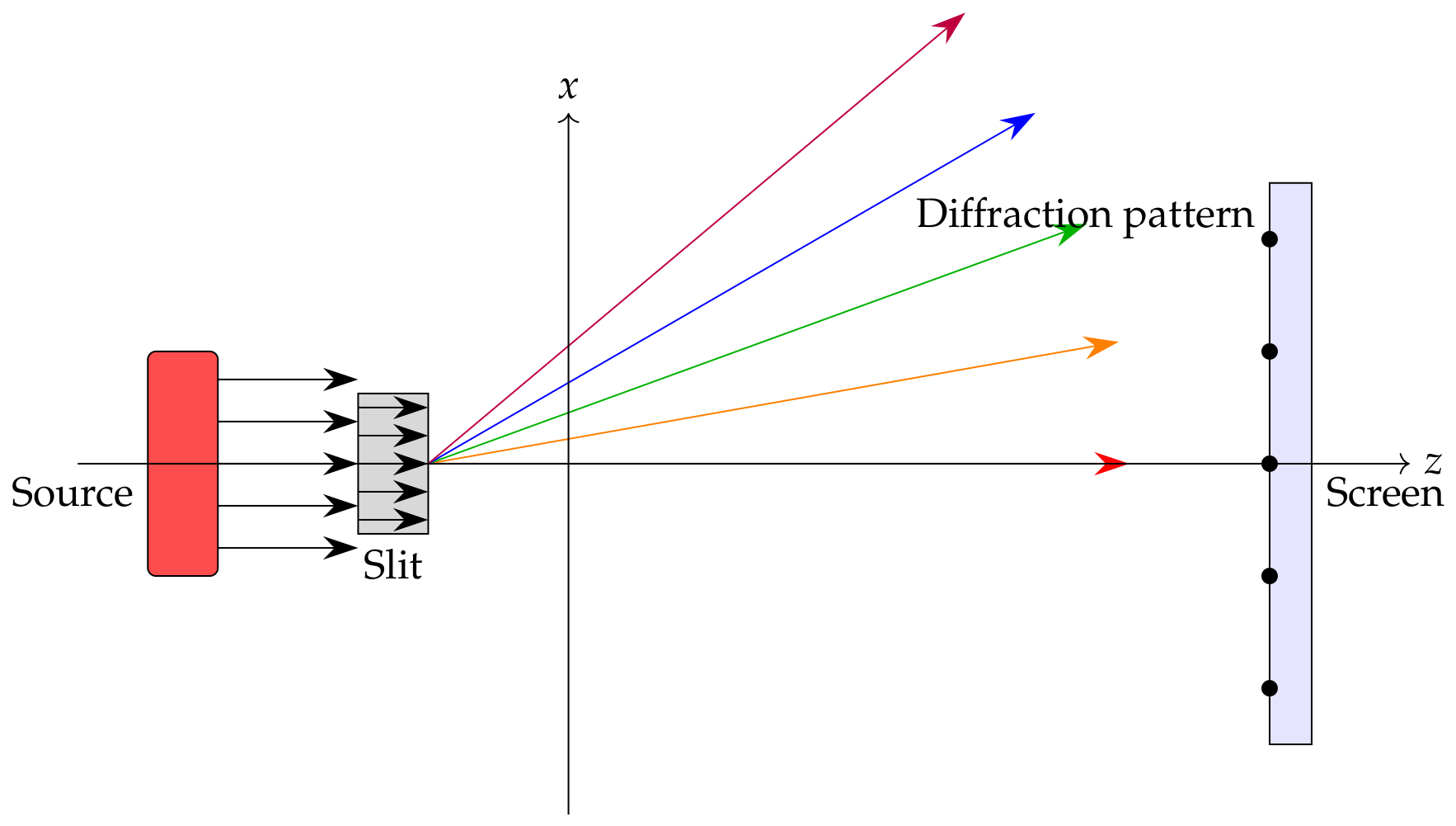
The Fraunhofer experimental setup is described in Figure 1. The diffraction of a light wave on a slit is observed in a far-field regime, i.e., when L, the distance along the z axis between the slit and the screen is much larger than the other length scales involved in the description of the diffraction. In this regime, the intensity along one axis on the screen for a monochromatic wave of wavelength is given as
with
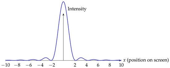
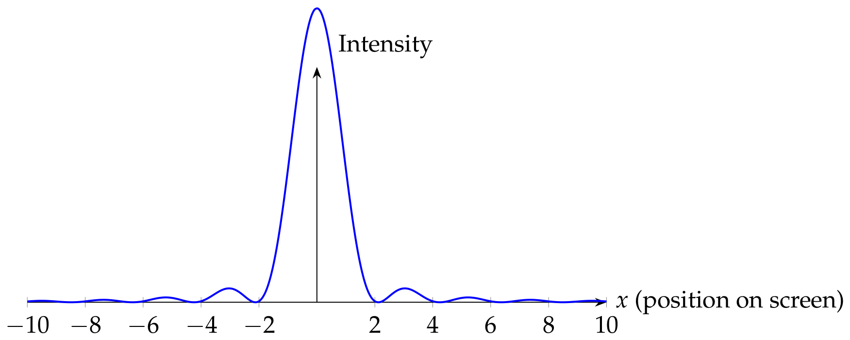
The intensity resulting from this interference phenomenon is illustrated in Figure 2. This result can be expressed in terms of the Fourier transform of the aperture as:
This result is the first in a series of scattering processes allowing us to connect the shape of the scattering target and a Fourier transform of the scattering figure.
Figure 1.
Scheme of Fraunhofer diffraction experimental setup. The coloured arrows show the directions of the scattered light.
Figure 2.
Fraunhofer diffraction pattern of a single rectangular slit.
The previous picture can be extended to a few orders of magnitude lower in wavelength. A typical example is X-ray diffraction on crystals. The periodic position of the atoms will create a typical periodic diffraction pattern, whose Fourier transform is once again related to the organisation of matter within the crystal.
Scattering can be used even at much lower length scales to probe the internal structure of matter. The famous example of the Rutherford experiment, in which particles are scattered on gold foil, invalidated the Thomson model (or plum pudding model) of the atom, paving the way for the planetary model.
2.2. Scaling the Idea Down to the Femtometer
The question we ask now is whether or not this idea can be pushed down to even lower length scales, in order to probe the content of the nucleon itself. Consider the following orders of magnitude:
- Typical nucleon radius: .
- To resolve structures of this size we need photons with , i.e., energies .
- The shortest laser wavelength obtained so far is still far from these scales.
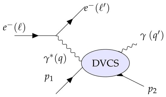
The issue of the photon source can be bypassed by looking at electron-proton scattering, where the content of the proton is probed by a highly virtual photon (see Figure 3). In such a configuration, the large virtuality can be experimentally controlled by selecting events whose recoiled electron momentum is such that is large compared to all other mass scales of the process. Then we can select events such that the proton remains intact through the process, and a final, real photon is also emitted. Such a process was suggested in ref. [3] and is known by the term DVCS.
Figure 3.
DVCS , where the incoming electron interacts with the nucleon through the exchange of a highly virtual photon .
In order to describe DVCS, which probes the Compton tensor in an off–forward kinematic configuration, we define the following momentum variables following ref. [1]:
Following an analysis “à la Brodsky–Lepage” [4], we will provide an intuitive, albeit non-rigorous, argument explaining why we can think about DVCS as the convolution of a local interaction between photons and partons, convoluted with a long-range matrix element bearing the information regarding the structure of the nucleon. The interested readers can find rigorous arguments regarding the factorisation of DVCS in [5,6,7].
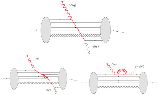
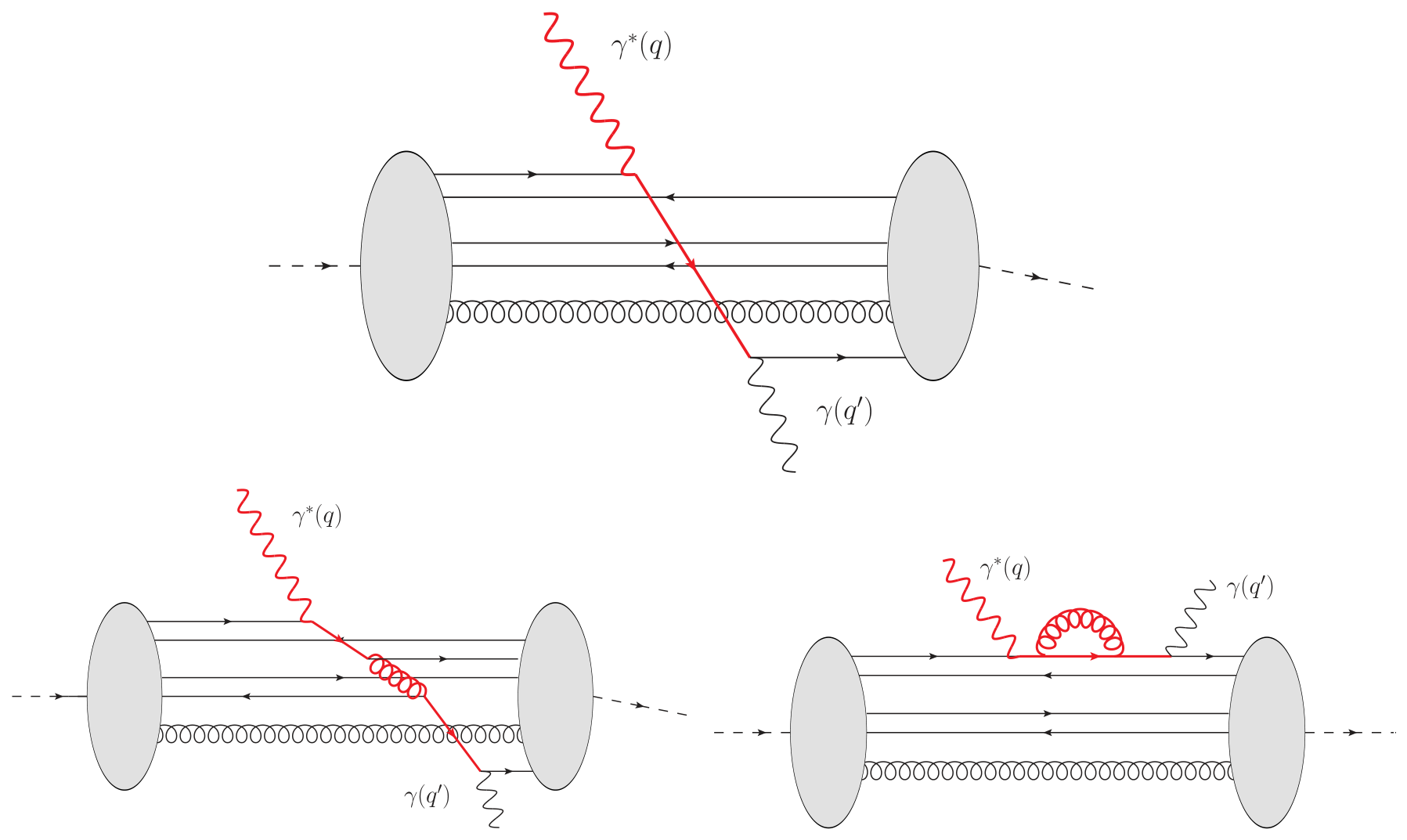
Following what happens in Deep Inelastic Scattering (DIS), the interaction of the nucleon with a highly virtual photon in DVCS selects configurations that are said to be “collinear”, i.e., where all constituents of the nucleon fly along the lightcone, carrying a longitudinal momentum fraction of the nucleon. The parton probed by the highly-virtual photon is then strongly shifted from this collinear direction (see top line of Figure 4). In order not to break the proton, the struck parton needs to release the off–forward momentum before reaching the edge of the proton (it needs to stay within the confinement range). This can be achieved by emitting a real photon, which yields the leading diagram describing the DVCS amplitude.
Figure 4.
Contributions to DVCS. On top, the leading contribution, in which the struck quark releases its “non-colinear” momentum by emitting a photon before escaping the “confinement range”, and thus breaking the proton.
Corrections to this leading case can be considered through the emission of gluons. Two types can be distinguished (bottom line of Figure 4). The first type is when the struck parton emits a gluon to release its off–forward momentum. The emitted gluon now becomes the highly virtual particle and needs to recombine with a quark before exiting the nucleon and thus breaking it. By doing so it transfers the off–forward momentum to the second quark, which itself needs to release it through a real photon. Such a contribution can thus be seen as a reshuffling of the off–forward momentum between the constituents of the nucleon. Because of the behaviour of the gluon propagator, one can show that it is power-suppressed in compared to the leading case.
Finally, the third contribution that one can consider is a loop correction to the propagation of the struck parton. Again, a hard gluon propagates, but since this time it is within a loop, all intermediate momentum degrees of freedom are integrated, leading to a logarithmic behaviour rather than a power suppression. There is no reshuffling of the momentum; this contribution has to be understood as a quantum correction to the propagation of the leading one. These logarithms can be computed using perturbation theory and resummed through evolution equations.
Finally, because of the power-suppressed reshuffling of the momentum, when is large, DVCS can be viewed as
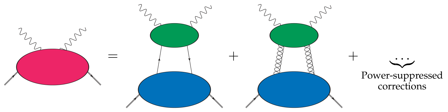 where the green ellipses are local interactions between the struck parton and the probe that can be computed in perturbation theory, while the blue ones encode non-perturbative physics and are parameterised in terms of GPDs.
In the following, we will provide a deeper study of GPDs. In Section 3, we will provide the definition and some basic properties of GPDs. Then in Section 4, we will explicitly show how to connect GPDs with the 3D number densities of partons within hadrons. The way GPDs are connected to the energy–momentum tensor will also be discussed. Both topics will come with more technical details that are usually not discussed in conferences, but I consider them important to keep in mind. Section 5 and Section 6 are more advanced, and suitable for students aiming at improving their detailed theoretical understanding of GPD physics. Finally, Section 7 explains how GPDs are connected to experimental processes and why it is challenging to extract them.
3. GPDs: Definitions and Properties
3.1. Formal Definitions of GPDs
GPDs were introduced independently in refs. [8,9,10] in the mid-1990s. They can be formally defined by looking at the tensor structure of the Fourier transform of a lightcone, off–forward matrix element
in the quark case. The integration runs over the lightcone separation , while the coordinates are fixed. The number of GPDs necessary to encode the information contained in a given matrix element depends on the spin of the targeted hadron. The higher the spin, the more GPDs are necessary. For the nucleon, other GPDs can be defined using other operators, such as polarised () or transversity () GPDs. But since I will not use them in the following, I will also skip introducing them. The interested reader can refer to ref. [1] for their definitions and properties.
Note that GPDs are Lorentz-invariant and that they also depend on three kinematic variables that are also Lorentz-invariant. We have already encountered , the Mandelstam variable. GPDs also depend on x, which is the Fourier conjugate to and stands for the average longitudinal momentum fraction carried by the probed parton. Note that . On the other hand, the skewness is half of the longitudinal momentum fraction transferred along the lightcone. Again, , although the kinematic phase space of DVCS probes only positive values of . Note that a Wilson line needs to be inserted to guarantee that the operator remains gauge-invariant. This Wilson line reduces to 1 in the specific case of the lightcone gauge.
Similarly to the quark sector, gluon GPDs can be defined as follows:
3.2. Properties of GPDs
The first property one would like to mention is the so-called forward limit, where (i.e., and ) such that the GPDs reduce to ordinary parton distribution functions (PDFs) q and g
where is the PDF of the quark flavour q, is the PDF of the antiquark of flavour q, and g is the gluon PDF.
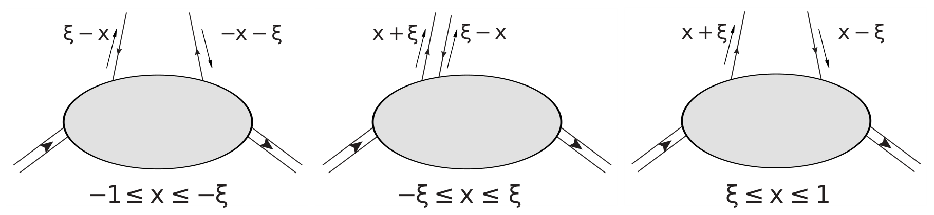
As illustrated in Figure 5, depending on the relative sign of , different interpretations can be built on the lightcone. Either one probes a quark in the kinematic area, an antiquark in the kinematic area or a pair of quark–antiquarks in the central area . The decomposition has important consequences, notably regarding the evolution equations driving the scale dependence of GPDs. Because of specific limits of these evolution equations, the outer regions are called the DGLAP regions, while the central region is called ERBL.
Figure 5.
Physical interpretation of the Dokshitzer–Gribov–Lipatov–Altarelli–Parisi (DGLAP) and Efremov–Radyushkin–Brodsky–Lepage (ERBL) regions.
Going back to Equation (6), we note that the matrix element defining GPDs would be the same as the one defining the electromagnetic form factors (EFFs) if we could make the operator local. This is achieved by integrating over x:
Thus, the first moment of GPDs yields the Dirac and Pauli EFF as:
Note that the first moment of GPDs is independent of . This can be derived from the polynomiality property we will discuss later on.
3.3. Experimental Connections
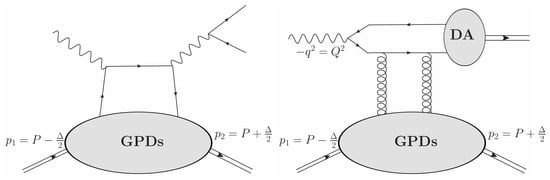
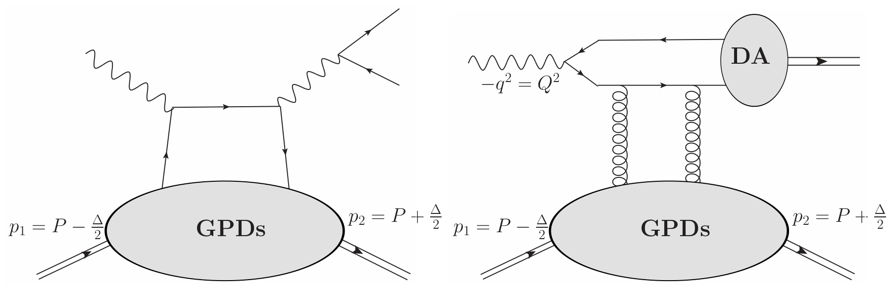
Several experimental processes are described in terms of GPDs, providing an experimental connection to these matrix elements. In addition to DVCS, already mentioned in the introduction, Deeply Virtual Meson Production (DVMP) and Timelike Compton Scattering (TCS) (see Figure 6) are also processes understood in the high limit in terms of GPDs. More details on how one can extract GPDs from exclusive processes (in particular DVCS) will be discussed in Section 7.
Figure 6.
Diagrammatic representation of TCS (left) and DVMP (right). Note that in the latter process, an additional non-perturbative object, the distribution amplitude, enters the description of the process.
4. Interpretation of GPDs
4.1. Probabilistic 1 + 2D Picture
In this section, we will prove that, as hinted in Section 2, GPDs contain the 1 + 2D number density of quarks and gluons within the nucleon, where 1 + 2D means 1D in momentum space and 2D in coordinate space (transverse plane). The analysis presented here mostly comes from ref. [11], though the first mention of the interpretation picture was made in ref. [12].
The first thing to ask before we discuss the connection between GPDs and spatial distribution of partons is how to define the centre of the nucleon in the transverse plane. The solution is provided by looking at a specific subclass of Lorentz boosts, called transverse boosts. These boosts are such that the component of the four-vector k is conserved, the transverse plane obeys Galilean transformation, and the component transform such that is left unchanged. Namely,
In the transverse plane, the transformation is formally the same as the so-called Galilean boosts [13], with playing the role of mass in Galilean transformation. This indicates that the non-relativistic centre of mass should be traded for the relativistic centre of + momentum defined as
where i labels the different components of the nucleon, is their momentum along the lightcone direction and their position in the transverse plane. This allows us to define a proton state whose centre of + momentum is localised at as:
Now, defining the transverse position dependent operator
one can show [11] that the following matrix element
corresponds to the amplitude of finding a quark at position in the transverse plane in a nucleon whose centre of plus momentum is shifted from to in the process. We immediately see that when , the matrix element becomes diagonal, and we recover a probabilistic interpretation. The number density can be expressed in terms of GPDs, by inserting (13) into (14). For a pion, one gets:
The resulting function gives the probability to find a parton with longitudinal momentum fraction x at transverse position relative to the centre of longitudinal momentum.
We note that this picture is significantly richer than the one coming from the EFF. First, it merges longitudinal momentum with the transverse plane position, thus providing a higher dimensional picture. Moreover, it also provides a way to map gluons within the nucleon, something that is out of reach at the level of the EFF.
4.2. Connection with the Energy–Momentum Tensor
In QCD, the energy–momentum tensor (EMT) matrix element is given as [14]
in its symmetric form. Note that the total EMT is scale-independent, and that different definitions and notations exist (The differences between canonical, kinematic and Belinfante EMT are discussed in detail in [14]. Belinfante EMT is the one presented here). We will stick to the present one. As in the case of GPDs, the number of EMT form factors necessary to parameterise the matrix element depends on the spin of the considered hadron. For the nucleon, four are necessary for the symmetric EMT. Constraints exist on these form factors:
- Because of momentum conservation, the total momentum fraction encoded in has to be 1. Thus:
- Because the total angular momentum , one should have:
- Because of the conservation of the total EMT, one obtains:
However, there is no constraint on C. Note that because the EMT is a conserved current, the properties highlighted in Equations (17)–(19) hold at any renormalisation scale and in any renormalisation scheme.
As previously, we will make a link between the EMT form factors and the GPDs through the integral over moments. Indeed, we note that the quark sector of the EMT is given by the operator
and where indicates that the operator is symmetrised and traceless. In the lightcone gauge, the covariant derivatives can be traded on the lightcone for the partial derivative. Going back again to Equation (6), and averaging over x, one gets:
where we now recognise the EMT operator in the quark sector, projected on the lightcone. Consequently the second moment of the GPDs maps directly onto the EMT form factors. The decomposition of the moment in terms of tensorial structures is performed, for instance, in [1]. Here we will just provide the result, which reads:
Consequently, in principle, if one can extract GPDs from experimental data (such as DVCS), one can also gain experimental access to the EMT form factors. Note again that this decomposition stems from the Lorentz structure of local operators and is independent of renormalisation scale or scheme. The scale and scheme dependence is to be found in the form factors , and .
From that point, the total angular momentum carried by quarks (or gluons) is obtained from H and E at zero-momentum transfer following Ji’s sum rule [9]:
On top of the Ji sum rules, mechanical properties of the nucleon can in principle be extracted from the form factor C [15]. However, one should keep in mind that the interpretation of the EMT form factor is frame-dependent. Indeed, we can look at the expression of the EMT in relativistic hydrodynamics [16,17]
where is the energy density, the radial pressure and the tangential pressure. From these quantities, one can define the so-called isotropic pressure p and the pressure anisotropy s as:
Following ref. [17], in the Breit frame, one can express the different pressure components and the energy density as for a parton type a:
As cannot be related to GPDs, only the total components of the energy and pressure can be extracted from DVCS, with the notable exception of the pressure anisotropy, which depends only on C and can be determined flavour by flavour.
5. Lorentz Covariance and Its Consequences
5.1. Mellin Moments as Local Matrix Elements
In this section we will start by generalising the study of Mellin moments; we started with the EFFs and EMT form factors. In the general case of a Mellin moment of order m, one has:
As one could have expected, the Mellin moments of GPDs can be expressed in terms of off–forward matrix elements of the local, twist-two operators. These operators are well-known and the same as in the PDF case:
However, due to the off–forward nature of the matrix element, we expect to get access to a richer tensorial structure for each moment. Proceeding with the tensorial decomposition of the matrix element, one sees that it can be parameterised using three types of form factors, A, B and C, weighting different tensorial structures. They are called generalised form factors and enter the decomposition of the matrix element as:
Using the Gordon identity
one can connect the generalised form factors with the moments of the GPDs H and E as:
This property is remarkable. Indeed, using simply the tensorial decomposition of the local matrix element, and its properties under Lorentz transformations, we have proven that the Mellin moments of GPDs are polynomials in of a degree controlled by the order of the Mellin moment computed [18,19].
From the connection between GPDs, PDFs, EFFs and the EMT, we can deduce the following properties:
- The are the moments of the PDF;
- is the Dirac form factor;
- is the Pauli form factor;
- The are the Mellin moments of a new object: the D-term.
5.2. The D-Term and the Radon Transform
Using the set of generalised form factors, we want to define a generating function D such that:
The question is now, how the variable y is connected with our physical momentum fractions x and . To answer this, we can rewrite the polynomiality property as:
where from the first to second line, we changed the variable such that , thereby answering the previous question. This provides us with another major outcome, namely that the D-term lives only in the so-called ERBL region. This depends only on two variables, just like the PDF, and we expect it to trigger some singular behaviours when (the limit depends on the direction in the ERBL region) and when .
Looking at Equation (41), we see that the structure has changed. By subtracting the D-term from the GPD, we find a polynomial in whose degree exactly matches the order of the selected Mellin moment. This has far-reaching consequences. Indeed, in mathematics, this relation is known as the Ludwig–Helgason consistency condition, and tells us that lives in the range of the Radon transform, i.e., there exists a function such that [20,21]
Reabsorbing the D-term into the integral, one can write
where we can now identify F with the Double Distribution (DD) [7,8] and D with the Polyakov–Weiss D-term [22].
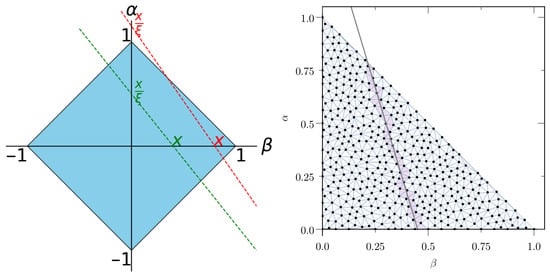
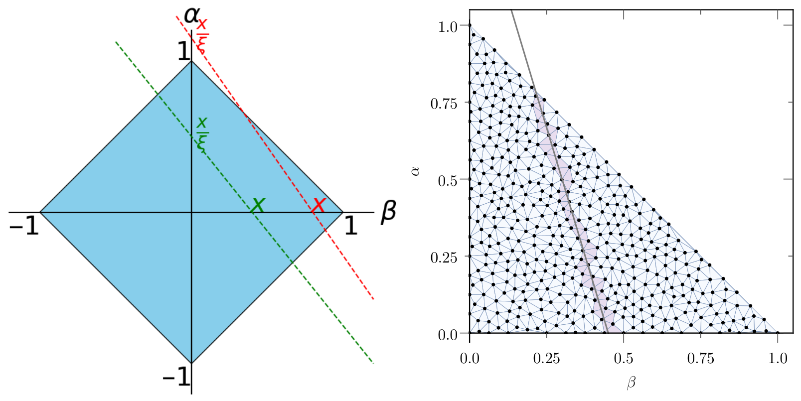
The properties of DDs are consistent with those of the GPDs. The support of on the one-ball (see Figure 7) guarantees the support in of the GPDs. The even parity in of the DD F guarantees the even parity in of the GPD. The generalised form factors can also be reinterpreted in terms of Mellin moments of the DD F:
Figure 7.
Double Distribution support crossed by lines of the type . Left-hand side: In red a DGLAP-type line, in green an ERBL-type line. Right-hand side: All cells of a discretised DD can be hit by infinitely many DGLAP-type lines, making the problem formally invertible.
A direct consequence is the link between the DD and the PDF:
Note that the same Radon representation applied to the GPD E, by introducing a DD usually labelled K:
5.3. Modelling Double Distributions
Double Distributions have enjoyed considerable success in attempts to model and extract GPDs, because they are in one-to-one correspondence with the polynomiality condition. Moreover, Musatov and Radyushkin developed an Ansatz that greatly facilitates the numerical implementation, and provides estimates based on the much better-known PDF [23]:
where is usually called the profile function. This model has been used under different forms in various analyses [24,25,26,27,28] and today remains an easy way to make assessments of experimental observations with the correct order of magnitude.
5.4. Addendum on Double Distributions
Some modern considerations developed in the last decade regarding Double Distributions are not available in the standard review papers in the field. Among them, let us mention the ability to fully determine the Double Distribution F by knowing the GPD solely in the DGLAP () region [21,29,30,31,32]. This was made possible by two key steps:
- The identification of the link between GPDs and DDs through the mathematically well-known Radon transform;
- The careful study of the mathematical properties of the incomplete Radon inverse problem and its consequences for compactly supported functions.
An intuitive picture can be built by looking at the discretised support of the DDs.
In this case, one can note that for each cell, it is possible to draw infinitely many DGLAP lines (i.e., lines that intersect the axis outside of the one-ball) hitting that cell. This means that, in principle, we can get infinitely many independent inputs coming from the DGLAP part of the GPDs to constrain the value of the DD on this cell (see Figure 7). This intuitively tells us that the incomplete inverse Radon problem is invertible. So far, this method has only been used to implement the GPDs model from Lightfront Wave Functions, but we expect it to play a significant role in future attempts to extract DDs from experimental data.
6. Evolution Equations of GPDs
In this section, we will briefly discuss the renormalisation and evolution equations of GPDs. This question has been studied since the 1990s, first at one loop [3,7,8], then two loops [33,34], and more recently three loops in the non-singlet case [35].
6.1. Renormalisation of Composite Operators
Returning to our matrix element definition of GPDs in Equation (6), one needs to realise that the matrix element is in fact singular in the limit , which is precisely the collinear limit in which we defined GPDs. In momentum space, this singularity is reached when one integrates over the transverse momentum degrees of freedom , and can thus be interpreted as a UV singularity. As usual, UV singularities are treated through the renormalisation programme. However, because the operator is a composite one, the simple renormalisation of the quark field as is not enough to remove the singularity of the non-local composite operators when approaching the lightcone. One needs to introduce a new renormalisation function that absorbs the singularities of the operator when . From that point, there are different ways to proceed, and we will briefly discuss only two: the OPE and renormalisation of local operators on the one hand, and the renormalisation of “in-partons” matrix elements in momentum space on the other hand.
Starting with the OPE approach, the idea is to “Taylor-expand” the operator as:
Then the dependence of in can be computed order by order in perturbation theory, together with the renormalisation constant of the local operator. Note that contrary to , does not depend on z, but one has to compute its general form for an arbitrary order of the expansion N. In other words, the z dependence is traded for an N dependence. Notwithstanding this difficulty, this formalism provides significant simplification as the renormalisation is multiplicative for all local operators, i.e., in momentum space, one handles products rather than convolutions. However it does not preclude some difficulties such as operator mixing, turning the renormalisation constant into “renormalisation matrices”.
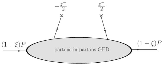
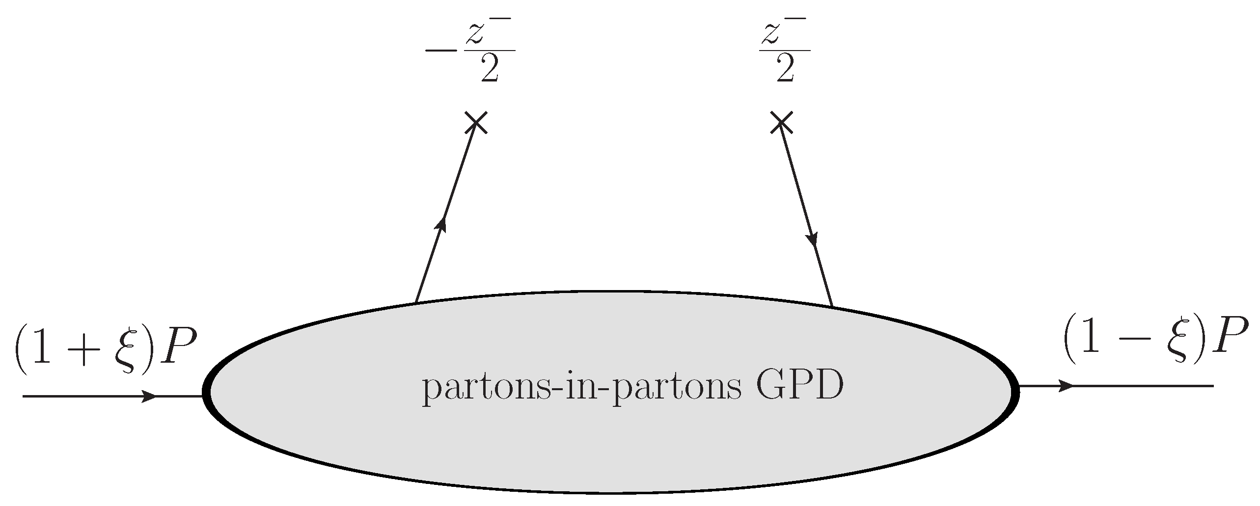
Another possibility is computing “in-partons” matrix elements (see Figure 8), i.e., to evaluate the operator contracted between states of partons with off-diagonal momenta. Trading a proton (or any hadron) state for a parton state is possible simply because the UV divergence is a universal property of the operator itself, and thus it does not depend on the nature of the incoming or outgoing state. This technique is described in great detail in ref. [36]. In the following, we will briefly describe such a method.
Figure 8.
In-parton GPDs that can be computed in pQCD.
The first thing to mention is that the computations are done in the scheme and in the lightcone gauge. The latter choice allows one to get rid of one-loop corrections coming from the Wilson line, at the price of introducing a more complicated gluon propagator. We are thus left with computing ladder graphs as those presented in Figure 9 and with self-energy-type graphs.
Figure 9.
Ladder graphs appearing in the renormalisation of the quark operator at one-loop in the lightcone gauge.
The computation then follows the standard rules when using the lightcone momentum decomposition:
- Integrate over to ensure momentum conservation;
- Integrate over using contour integration and the residue theorem;
- Integrate over in such that the poles in and its residue can be identified.
Once all computations are performed, the result takes the form of
where Z is the momentum-dependent renormalisation “function” of the GPD.
6.2. Evolution Equations
The result obtained in Equation (51) is interesting but cannot be directly used. Indeed, one cannot compute for a nucleon. Moreover, we expect that the validity will be rather restricted to a small range in as large logarithmic corrections may spoil this simple one-loop result. Fortunately, these logarithmic corrections can be resummed by using the Callan–Symanzik equation. To do so, we start by considering a small variation of the scale
and then take the logarithmic derivatives as:
Now inverting Equation (51) to get as a convolution of and H, we obtain a first-order integro-differential equation
where is the splitting function, the formal generalisation of the anomalous dimension in the Callan–Symanzik equation, and is given by:
Note that because of the first-order structure of the equation, the -dependence becomes “exponentiated” in the solution of this equation. This is critical, as it means that solving this equation resums a series of powers of , increasing the validity of the one-loop computation far beyond its initial range when simply computing Z.
Finally, let us discuss mixing between quark and gluon contributions. Figure 9 shows an example of an off-diagonal contribution, where a quark operator is evaluated between gluon states. In fact one can decompose the quark contribution into singlet and non-singlet combinations. Only the singlet combination will mix with gluons. We are thus left in the non-singlet sector with
where is the one-loop “quark-in-quark” splitting function. In the singlet case, the scalar structure of Equation (56) is replaced by a vector:
In this two-by-two splitting matrix, all terms can in principle be computed in perturbation theory. The explicit expression of the splitting function is not important for the following discussion, but can be found in a numerical implementation-friendly form in ref. [36].
Let us now discuss some limiting cases. Since the forward limit of the GPDs is given in terms of PDFs, we expect that the limit of the GPD splitting functions yields the DGLAP ones [37,38,39]:
Another limit can be identified, this time when . In this specific case, on the entire kinematic range, the GPD is interpreted as a quark–antiquark pair, just like in distribution amplitudes. We thus expect to recover the ERBL [4,40,41,42] and Chase [43] evolution kernels, and this is indeed what happens:
The reason why GPDs bridge the gap between DGLAP and ERBL evolution is simply that the operator considered is the same, and thus develops the same UV divergences when evaluated in the same kinematic configurations, regardless of the type of state that is probed. An illustration of this is readily given when looking at the anomalous dimensions of the evolution kernel. They are simpler to define when one rewrites Equation (54) as
where can be deduced from (see ref. [36]). Then we can define the eigenvalues and eigenvectors of as
We deduce from that, that the anomalous dimensions of the local operators diagonalising the non-singlet evolution kernel, are the same as the DGLAP and ERBL ones:
The eigenvectors , however, are different. They are given by the Gegenbauer- polynomials
which in the limit give back the monomials diagonalising the DGLAP equations and in the limit the standard diagonalising the ERBL evolution equation. The evolution of the conformal moments is thus given as
similarly to the Mellin moments of PDFs.
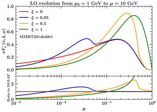
We will conclude this section with some numerical considerations. The simple evolution for conformal moments in Equation (64) is in fact challenging to invert, as an analytic continuation for , is needed; otherwise, the result is not unique [44]. On the other hand, numerically solving Equation (57) is fast and stable on modern computers, favouring (at least at one loop) this approach as illustrated in Figure 10.
Figure 10.
Example taken from ref. [36] of a numerical solution of the GPD evolution equations for various values of . Note that the evolution equation generates a cusp at .
We note that the evolution equations preserve the continuity at , which is a key condition to allow DVCS amplitude to be factorised. However, we also point out that a cusp is generated, and it comes from the different kinematic configurations between the DGLAP and ERBL region, making the splitting functions themselves non-differentiable at that point. However, this has no consequences on the most common exclusive processes.
7. Probing GPDs Through Exclusive Processes
For a more complete modern picture on this topic, I recommend reading the Ph.D. thesis by H. Dutrieux [45].
7.1. Extracting DVCS Amplitude
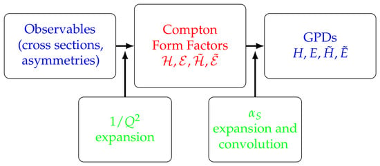
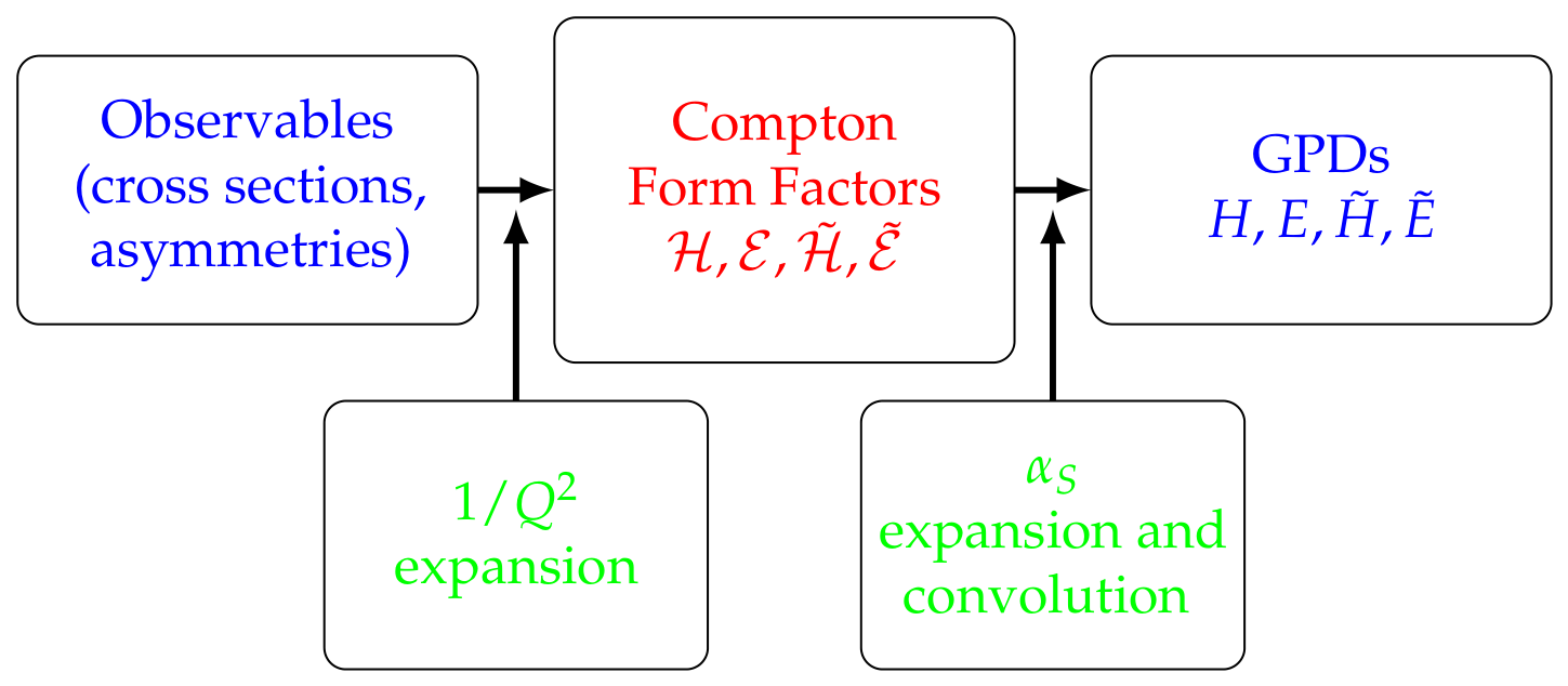
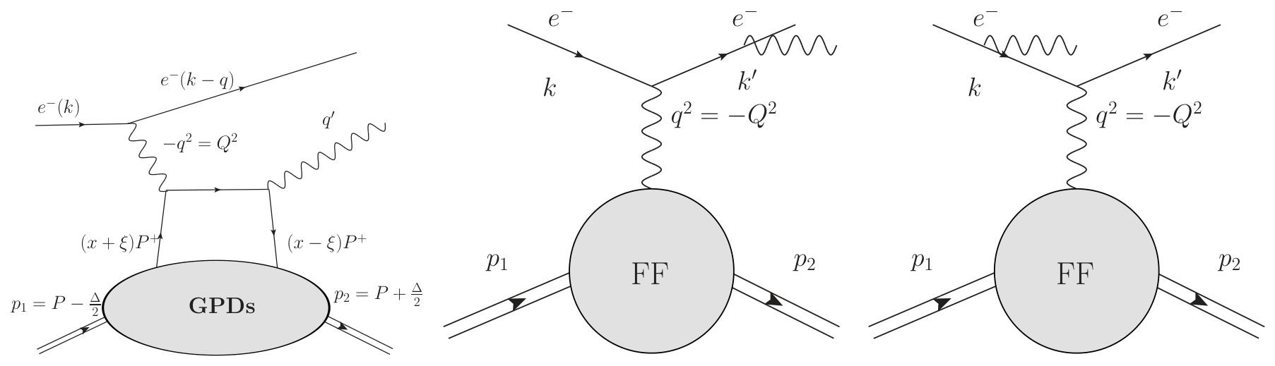
Unlike inclusive processes, where the cross section is directly connected to PDFs through the optical theorem, exclusive processes factorise at the amplitude level. Consequently, as illustrated in Figure 11, connecting GPDs to experimental data is a two-step process, with the computation or extraction of the amplitude acting as an intermediate step. This step is already challenging in itself, especially for DVCS, as at the level of cross sections, all processes with the same final state interfere. In the photon electroproduction case , DVCS competes with another process called the Bethe–Heitler process, in which the final photon is emitted by the Bremsstrahlung of the incoming or outgoing electron rather than by partons within the nucleon (see Figure 12).
Figure 11.
Structure connecting GPDs to experimental data.
Figure 12.
Diagrams of Bethe–Heitler and DVCS processes interfering in the process .
We are thus left with a cross section that is schematically written in terms of the amplitudes of the processes as
Moreover, the pure DVCS term is suppressed in with respect to the pure Bethe–Heitler term. The natural experimental goal is thus to characterise the interference term which is less suppressed (by ) than the pure DVCS one. This strategy is simplified by measuring the so-called beam-spin asymmetry, which directly probes the interference term. Before proceeding, one should realise that the total DVCS amplitude can be either decomposed in terms of helicity amplitudes (i.e., on the projection of photon and hadron helicities), or in terms of Compton Form Factors (CFFs), which encodes the non-perturbative content associated with a given tensorial structure. For example, the CFF is associated with the tensorial structure (which is the one attached to the GPD H, hence the notations). The definition of CFFs and the helicity amplitudes can be found, for instance, in [1]. The observable beam spin asymmetry has allowed various collaborations to extract GPDs with reasonable control of the imaginary part of the DVCS amplitude, and more precisely the Compton Form Factor dominating the DVCS process when the helicity of the photon and of the proton are conserved through the scattering. Global extractions can be found in refs. [46,47,48].
7.2. Extraction of GPDs
The CFFs are then expressed as a convolution between a scattering coefficient function computed in perturbation theory C and the associated GPDs. Typically one writes:
For DVCS, C has been computed up to next-to-next-to-leading order [49] and next-to-next-to-leading kinematic power [50]. However, at leading order and leading power, the imaginary part of C simply yields:
This form is problematic because it has an obvious kernel, i.e., an obvious subset of functions such that their convolution with will give zero. These functions are the ones vanishing on the diagonal . From this statement, one should ask whether this is still the case when the computation is refined by higher orders of or kinematic power corrections. The answer is yes, as shown in ref. [51], and can be understood through the concept of shadow GPDs. A candidate shadow GPD at order n in is a function fulfilling all theoretical properties of GPDs, and such that:
In order to find shadow GPDs, it is convenient to look for shadow DDs, as polynomiality is fulfilled by construction. A simple way to construct solutions is thus to look at
and expand on monomials of the type up to a maximal degree N. This provides a number of parameters that scale like . However, it involves adding the following constraints:
- The forward limit goes to zero;
- The imaginary part of the CFF goes to zero;
- The DD is continuous on the edges of the one-ball.
This provides sets of constraints that only scale like N. A shadow distribution is thus found at the LO of the coefficient function for and at NLO for .
Evolution equations were thought to be a solution to this problem, as they mix shadow GPDs with “detectable” GPDs [52]. However, in practice this is not the case, as the impact of shadow GPDs is still times smaller than of regular GPDs, even when evolving over a large lever arm in .
The strategy to bypass shadow GPDs can take several forms. In addition to DVCS, seep exclusive meson production also suffers from the shadow GPD problem. However, one idea is to realise that shadow GPDs are process-dependent, and thus performing a multi-channel extraction helps reduce the overall kernel. Even better, some channels, such as Double DVCS [53,54] or deep exclusive processes [55,56,57,58,59,60], are expected not to suffer from the shadow GPD problem. Although much harder to detect, they may nevertheless help constrain the inverse problem.
Another suggested possibility is to build models fulfilling by construction the positivity property [61,62,63]. Such a property, not mentioned in this document, strongly helps to mitigate the shadow GPD problem, as it reduces the ability of the model to fluctuate in the DGLAP region [64].
Lattice QCD has also been proposed as a possibility for solving the problem. While it does help, because one probes only low Fourier modes, the reduction of uncertainties due to the shadow space is noticeable but not dramatic [65]. In the best case, uncertainties are expected to be reduced by a factor of two.
Note that some collaborations have nevertheless extracted GPD models by strongly reducing the dimensionality of their own modelling strategy, and thus introducing significant bias [24,26,66,67,68], without taking into account the shadow GPD problem. Different tools are publicly available to perform GPDs analysis, such as PARTONS [69] and GeParD [70]. To date, however, no satisfactory solution has been implemented.
8. Conclusions
In these lecture notes I introduced the idea of using light scattering to determine experimentally the internal structure of the nucleon. We saw that deep exclusive processes allow one to perform such a task, as they factorise in terms of a local coefficient function describing the interaction between the probe and the struck parton, and the multidimensional structure of the nucleon encoded in GPDs. We discussed the various theoretical properties of GPDs, and their connection with better-known functions such as the EFF or the PDFs. Finally we discussed the practical ways to extract these GPDs from experimental data, and highlighted the real difficulties that preclude a reliable extraction of the latter today. This problem remains open today despite the numerous works dedicated to the topic.
Funding
This research received no external funding.
Institutional Review Board Statement
Not applicable.
Informed Consent Statement
Not applicable.
Data Availability Statement
No new data were created or analyzed in this study. Data sharing is not applicable to this article.
Acknowledgments
I am grateful to the Institute of Non-perturbative Physics (INP) of Nanjing University for their invitation to the International Workshop and School on Hadron Structure & Strong Interactions.
Conflicts of Interest
The author declares no conflicts of interest.
References
- Diehl, M. Generalized parton distributions. Phys. Rep. 2003, 388, 41–277. [Google Scholar] [CrossRef] [Scilit]
- Belitsky, A.; Radyushkin, A. Unraveling hadron structure with generalized parton distributions. Phys. Rep. 2005, 418, 1–387. [Google Scholar] [CrossRef] [Scilit]
- Ji, X.D. Deeply virtual Compton scattering. Phys. Rev. D 1997, 55, 7114–7125. [Google Scholar] [CrossRef] [Scilit]
- Lepage, G.P.; Brodsky, S.J. Exclusive Processes in Perturbative Quantum Chromodynamics. Phys. Rev. D 1980, 22, 2157. [Google Scholar] [CrossRef] [Scilit]
- Ji, X.D.; Osborne, J. One loop corrections and all order factorization in deeply virtual Compton scattering. Phys. Rev. D 1998, 58, 094018. [Google Scholar] [CrossRef] [Scilit]
- Collins, J.C.; Freund, A. Proof of factorization for deeply virtual Compton scattering in QCD. Phys. Rev. D 1999, 59, 074009. [Google Scholar] [CrossRef] [Scilit]
- Radyushkin, A. Nonforward parton distributions. Phys. Rev. D 1997, 56, 5524–5557. [Google Scholar] [CrossRef] [Scilit]
- Mueller, D.; Robaschik, D.; Geyer, B.; Dittes, F.; Hořeǰsi, J. Wave functions, evolution equations and evolution kernels from light ray operators of QCD. Fortschr. Phys. 1994, 42, 101–141. [Google Scholar] [CrossRef] [Scilit]
- Ji, X.D. Gauge-Invariant Decomposition of Nucleon Spin. Phys. Rev. Lett. 1997, 78, 610–613. [Google Scholar] [CrossRef] [Scilit]
- Radyushkin, A. Scaling limit of deeply virtual Compton scattering. Phys. Lett. B 1996, 380, 417–425. [Google Scholar] [CrossRef] [Scilit]
- Diehl, M. Generalized parton distributions in impact parameter space. Eur. Phys. J. C 2002, 25, 223–232. [Google Scholar] [CrossRef] [Scilit]
- Burkardt, M. Impact parameter dependent parton distributions and off forward parton distributions for 0. Phys. Rev. D 2000, 62, 071503, Erratum in Phys. Rev. D 2002, 66, 119903. https://doi.org/10.1103/PhysRevD.66.119903. [Google Scholar] [CrossRef] [Scilit]
- Susskind, L. Model of self-induced strong interactions. Phys. Rev. 1968, 165, 1535–1546. [Google Scholar] [CrossRef] [Scilit]
- Leader, E.; Lorcé, C. The angular momentum controversy: What’s it all about and does it matter? Phys. Rep. 2014, 541, 163–248. [Google Scholar] [CrossRef] [Scilit]
- Polyakov, M.V. Generalized parton distributions and strong forces inside nucleons and nuclei. Phys. Lett. B 2003, 555, 57–62. [Google Scholar] [CrossRef] [Scilit]
- Bayin, S.S. Anisotropic fluids and cosmology. Astrophys. J. 1986, 303, 101–110. [Google Scholar] [CrossRef] [Scilit] [PubMed]
- Lorcé, C.; Moutarde, H.; Trawiński, A.P. Revisiting the mechanical properties of the nucleon. Eur. Phys. J. C 2019, 79, 89. [Google Scholar] [CrossRef] [Scilit]
- Ji, X.D. Off forward parton distributions. J. Phys. G 1998, 24, 1181–1205. [Google Scholar] [CrossRef] [Scilit]
- Radyushkin, A. Symmetries and structure of skewed and double distributions. Phys. Lett. B 1999, 449, 81–88. [Google Scholar] [CrossRef] [Scilit]
- Teryaev, O. Crossing and radon tomography for generalized parton distributions. Phys. Lett. B 2001, 510, 125–132. [Google Scholar] [CrossRef] [Scilit]
- Chouika, N.; Mezrag, C.; Moutarde, H.; Rodríguez-Quintero, J. Covariant Extension of the GPD overlap representation at low Fock states. Eur. Phys. J. C 2017, 77, 906. [Google Scholar] [CrossRef] [Scilit]
- Polyakov, M.V.; Weiss, C. Skewed and double distributions in pion and nucleon. Phys. Rev. D 1999, 60, 114017. [Google Scholar] [CrossRef] [Scilit]
- Musatov, I.; Radyushkin, A. Evolution and models for skewed parton distributions. Phys. Rev. D 2000, 61, 074027. [Google Scholar] [CrossRef] [Scilit]
- Vanderhaeghen, M.; Guichon, P.A.; Guidal, M. Deeply virtual electroproduction of photons and mesons on the nucleon: Leading order amplitudes and power corrections. Phys. Rev. D 1999, 60, 094017. [Google Scholar] [CrossRef] [Scilit]
- Guidal, M.; Polyakov, M.; Radyushkin, A.; Vanderhaeghen, M. Nucleon form-factors from generalized parton distributions. Phys. Rev. D 2005, 72, 054013. [Google Scholar] [CrossRef] [Scilit]
- Goloskokov, S.; Kroll, P. The Role of the quark and gluon GPDs in hard vector-meson electroproduction. Eur. Phys. J. C 2008, 53, 367–384. [Google Scholar] [CrossRef] [Scilit]
- Goloskokov, S.; Kroll, P. The Longitudinal cross-section of vector meson electroproduction. Eur. Phys. J. C 2007, 50, 829–842. [Google Scholar] [CrossRef] [Scilit]
- Mezrag, C.; Moutarde, H.; Sabatié, F. Test of two new parameterizations of the Generalized Parton Distribution H. Phys. Rev. D 2013, 88, 014001. [Google Scholar] [CrossRef] [Scilit]
- Chouika, N.; Mezrag, C.; Moutarde, H.; Rodríguez-Quintero, J. A Nakanishi-based model illustrating the covariant extension of the pion GPD overlap representation and its ambiguities. Phys. Lett. B 2018, 780, 287–293. [Google Scholar] [CrossRef] [Scilit]
- Chavez, J.M.M.; Bertone, V.; De Soto Borrero, F.; Defurne, M.; Mezrag, C.; Moutarde, H.; Rodríguez-Quintero, J.; Segovia, J. Pion generalized parton distributions: A path toward phenomenology. Phys. Rev. D 2022, 105, 094012. [Google Scholar] [CrossRef] [Scilit]
- Chávez, J.M.M.; Bertone, V.; De Soto Borrero, F.; Defurne, M.; Mezrag, C.; Moutarde, H.; Rodríguez-Quintero, J.; Segovia, J. Accessing the Pion 3D Structure at US and China Electron-Ion Colliders. Phys. Rev. Lett. 2022, 128, 202501. [Google Scholar] [CrossRef] [Scilit] [PubMed]
- Dall’Olio, P.; De Soto, F.; Mezrag, C.; Morgado Chávez, J.M.; Moutarde, H.; Rodríguez-Quintero, J.; Sznajder, P.; Segovia, J. Unraveling generalized parton distributions through Lorentz symmetry and partial DGLAP knowledge. Phys. Rev. D 2024, 109, 096013. [Google Scholar] [CrossRef] [Scilit]
- Belitsky, A.V.; Freund, A.; Mueller, D. Evolution kernels of skewed parton distributions: Method and two loop results. Nucl. Phys. B 2000, 574, 347–406. [Google Scholar] [CrossRef] [Scilit]
- Braun, V.M.; Manashov, A.N.; Moch, S.; Strohmaier, M. Two-loop evolution equations for flavor-singlet light-ray operators. J. High Energy Phys. 2019, 2019, 191. [Google Scholar] [CrossRef] [Scilit]
- Braun, V.M.; Manashov, A.N.; Moch, S.; Strohmaier, M. Three-loop evolution equation for flavor-nonsinglet operators in off-forward kinematics. J. High Energy Phys. 2017, 2017, 37. [Google Scholar] [CrossRef] [Scilit]
- Bertone, V.; Dutrieux, H.; Mezrag, C.; Morgado, J.M.; Moutarde, H. Revisiting evolution equations for generalised parton distributions. Eur. Phys. J. C 2022, 82, 888. [Google Scholar] [CrossRef] [Scilit]
- Dokshitzer, Y.L. Calculation of the Structure Functions for Deep Inelastic Scattering and e+ e− Annihilation by Perturbation Theory in Quantum Chromodynamics. Sov. Phys. JETP 1977, 46, 641–653. [Google Scholar]
- Gribov, V.; Lipatov, L. Deep inelastic e p scattering in perturbation theory. Sov. J. Nucl. Phys. 1972, 15, 438–450. [Google Scholar]
- Altarelli, G.; Parisi, G. Asymptotic Freedom in Parton Language. Nucl. Phys. B 1977, 126, 298. [Google Scholar] [CrossRef] [Scilit]
- Efremov, A.; Radyushkin, A. Asymptotical Behavior of Pion Electromagnetic Form-Factor in QCD. Theor. Math. Phys. 1980, 42, 97–110. [Google Scholar] [CrossRef] [Scilit]
- Efremov, A.; Radyushkin, A. Factorization and Asymptotical Behavior of Pion Form-Factor in QCD. Phys. Lett. B 1980, 94, 245–250. [Google Scholar] [CrossRef] [Scilit]
- Lepage, G.P.; Brodsky, S.J. Exclusive Processes in Quantum Chromodynamics: Evolution Equations for Hadronic Wave Functions and the Form-Factors of Mesons. Phys. Lett. B 1979, 87, 359–365. [Google Scholar] [CrossRef] [Scilit]
- Chase, M.K. The Q2 evolution of flavor singlet wave functions in QCD. Nucl. Phys. B 1980, 174, 109–122. [Google Scholar] [CrossRef] [Scilit]
- Mueller, D.; Schafer, A. Complex conformal spin partial wave expansion of generalized parton distributions and distribution amplitudes. Nucl. Phys. B 2006, 739, 1–59. [Google Scholar] [CrossRef] [Scilit]
- Dutrieux, H. Phenomenology of Generalised Parton Distributions from Deeply Virtual Compton Scattering. Ph.D. Thesis, IRFU, Saclay, France, 2022. [Google Scholar]
- Moutarde, H.; Sznajder, P.; Wagner, J. Unbiased determination of DVCS Compton Form Factors. Eur. Phys. J. C 2019, 79, 614. [Google Scholar] [CrossRef] [Scilit]
- Čuić, M.; Kumerički, K.; Schäfer, A. Separation of Quark Flavors Using Deeply Virtual Compton Scattering Data. Phys. Rev. Lett. 2020, 125, 232005. [Google Scholar] [CrossRef] [Scilit] [PubMed]
- Almaeen, M.; Alghamdi, T.; Kriesten, B.; Adams, D.; Li, Y.; Lin, H.W.; Liuti, S. VAIM-CFF: A variational autoencoder inverse mapper solution to Compton form factor extraction from deeply virtual exclusive reactions. Eur. Phys. J. C 2025, 85, 499. [Google Scholar] [CrossRef] [Scilit]
- Braun, V.M.; Ji, Y.; Schoenleber, J. Deeply Virtual Compton Scattering at Next-to-Next-to-Leading Order. Phys. Rev. Lett. 2022, 129, 172001. [Google Scholar] [CrossRef] [Scilit] [PubMed]
- Braun, V.M.; Ji, Y.; Manashov, A.N. Kinematic power corrections to deeply virtual Compton scattering to twist-six accuracy. Phys. Rev. D 2025, 111, 076011. [Google Scholar] [CrossRef] [Scilit]
- Bertone, V.; Dutrieux, H.; Mezrag, C.; Moutarde, H.; Sznajder, P. The deconvolution problem of deeply virtual Compton scattering. Phys. Rev. D 2021, 103, 114019. [Google Scholar] [CrossRef] [Scilit]
- Freund, A. On the extraction of skewed parton distributions from experiment. Phys. Lett. B 2000, 472, 412–419. [Google Scholar] [CrossRef] [Scilit]
- Guidal, M.; Vanderhaeghen, M. Double deeply virtual Compton scattering off the nucleon. Phys. Rev. Lett. 2003, 90, 012001. [Google Scholar] [CrossRef] [Scilit] [PubMed]
- Deja, K.; Martinez-Fernandez, V.; Pire, B.; Sznajder, P.; Wagner, J. Phenomenology of double deeply virtual Compton scattering in the era of new experiments. Phys. Rev. D 2023, 107, 094035. [Google Scholar] [CrossRef]
- Boussarie, R.; Pire, B.; Szymanowski, L.; Wallon, S. Exclusive photoproduction of a γρ pair with a large invariant mass. J. High Energy Phys. 2017, 2017, 54, Erratum in J. High Energy Phys. 2018, 10, 29. [Google Scholar] [CrossRef] [Scilit]
- Grocholski, O.; Pire, B.; Sznajder, P.; Szymanowski, L.; Wagner, J. Collinear factorization of diphoton photoproduction at next to leading order. Phys. Rev. D 2021, 104, 114006. [Google Scholar] [CrossRef] [Scilit]
- Grocholski, O.; Pire, B.; Sznajder, P.; Szymanowski, L.; Wagner, J. Phenomenology of diphoton photoproduction at next-to-leading order. Phys. Rev. D 2022, 105, 094025. [Google Scholar] [CrossRef] [Scilit]
- Qiu, J.W.; Yu, Z. Exclusive production of a pair of high transverse momentum photons in pion-nucleon collisions for extracting generalized parton distributions. J. High Energy Phys. 2022, 2022, 103. [Google Scholar] [CrossRef] [Scilit]
- Qiu, J.W.; Yu, Z. Extraction of the Parton Momentum-Fraction Dependence of Generalized Parton Distributions from Exclusive Photoproduction. Phys. Rev. Lett. 2023, 131, 161902. [Google Scholar] [CrossRef] [Scilit] [PubMed]
- Duplančić, G.; Nabeebaccus, S.; Passek-Kumerički, K.; Pire, B.; Szymanowski, L.; Wallon, S. Probing chiral-even and chiral-odd leading twist quark generalized parton distributions through the exclusive photoproduction of a γρ pair. Phys. Rev. D 2023, 107, 094023. [Google Scholar] [CrossRef] [Scilit]
- Diehl, M.; Feldmann, T.; Jakob, R.; Kroll, P. The Overlap representation of skewed quark and gluon distributions. Nucl. Phys. B 2001, 596, 33–65. [Google Scholar] [CrossRef] [Scilit]
- Pobylitsa, P. Disentangling positivity constraints for generalized parton distributions. Phys. Rev. D 2002, 65, 114015. [Google Scholar] [CrossRef] [Scilit]
- Pobylitsa, P. Inequalities for generalized parton distributions H and E. Phys. Rev. D 2002, 65, 077504. [Google Scholar] [CrossRef] [Scilit]
- Dutrieux, H.; Dutrieux, H.; Grocholski, O.; Grocholski, O.; Moutarde, H.; Moutarde, H.; Sznajder, P.; Sznajder, P. Artificial neural network modelling of generalised parton distributions. Eur. Phys. J. C 2022, 82, 252, Erratum in Eur. Phys. J. C 2022, 82, 389. [Google Scholar] [CrossRef] [Scilit]
- Riberdy, M.J.; Dutrieux, H.; Mezrag, C.; Sznajder, P. Combining lattice QCD and phenomenological inputs on generalised parton distributions at moderate skewness. Eur. Phys. J. C 2024, 84, 201. [Google Scholar] [CrossRef] [Scilit]
- Moutarde, H.; Sznajder, P.; Wagner, J. Border and skewness functions from a leading order fit to DVCS data. Eur. Phys. J. C 2018, 78, 890. [Google Scholar] [CrossRef] [Scilit]
- Čuić, M.; Duplančić, G.; Kumerički, K.; Passek-K, K. NLO corrections to the deeply virtual meson production revisited: Impact on the extraction of generalized parton distributions. J. High Energy Phys. 2023, 2023, 192, Erratum in J. High Energy Phys. 2024, 2, 225. [Google Scholar] [CrossRef] [Scilit]
- Guo, Y.; Aslan, F.P.; Ji, X.; Santiago, M.G. First Global Extraction of Generalized Parton Distributions from Experiment and Lattice Data with Next-to-Leading-Order Accuracy. Phys. Rev. Lett. 2025, 135, 261903. [Google Scholar] [CrossRef] [Scilit] [PubMed]
- Berthou, B.; Binosi, D.; Chouika, N.; Colaneri, L.; Guidal, M.; Mezrag, C.; Moutarde, H.; Rodríguez-Quintero, J.; Sabatié, F.; Sznajder, P.; et al. PARTONS: PARtonic Tomography Of Nucleon Software. A computing framework for the phenomenology of Generalized Parton Distributions. Eur. Phys. J. C 2018, 78, 478. [Google Scholar] [CrossRef] [Scilit]
- Kumerički, K.; Müller, D. Description and interpretation of DVCS measurements. EPJ Web Conf. 2016, 112, 01012. [Google Scholar] [CrossRef] [Scilit]


Disclaimer/Publisher’s Note: The statements, opinions and data contained in all publications are solely those of the individual author(s) and contributor(s) and not of MDPI and/or the editor(s). MDPI and/or the editor(s) disclaim responsibility for any injury to people or property resulting from any ideas, methods, instructions or products referred to in the content. |
© 2026 by the author. Licensee MDPI, Basel, Switzerland. This article is an open access article distributed under the terms and conditions of the Creative Commons Attribution (CC BY) license.