


Abstract
Precision agriculture and sustainable farming practices require autonomous environmental monitoring systems capable of operating in remote areas with limited energy and connectivity. However, the high cost of existing professional technology remains a significant barrier to widespread adoption. This study presents the development of a solar-powered smart sensing node designed for autonomous operation that integrates TinyML and dual-mode wireless connectivity via LoRaWAN and Wi-Fi for intelligent monitoring. The system features a custom-designed cup anemometer and multispectral sensing capabilities integrated into a compact single-tower architecture. All structural components, including radiation shields and a modular PVC frame, were designed for low-cost manufacturing and mass production. A single hermetic housing protects the core control electronics and is designed to improve durability in harsh outdoor environments. A Multi-Layer Perceptron model was implemented on the edge to enable intelligent data fusion and compensation, while a dynamic sampling strategy optimized power consumption. Experimental results demonstrate the feasibility of the proposed architecture through adaptive spectral acquisition over a daily illumination cycle, embedded MLP-based sensor fusion, and telemetry-oriented data compression that substantially reduces the number of transmitted samples. The main contribution of this work is a system-level architecture that integrates sensing, embedded intelligence, solar-energy harvesting, hybrid wireless communication, and telemetry optimization into a compact, low-cost, and field-deployable prototype IoT platform for sustainable precision agriculture.
Keywords:
TinyML; LoRaWAN; precision agriculture; solar-powered; IoT; environmental monitoring; Wi-Fi 1. Introduction
Traditional agriculture faces severe climatic demands that limit crop yields, and population growth is putting unprecedented pressure on land resources. Due to the scarcity of land and water, facility-based agriculture, such as smart greenhouses and plant factories, has gained prominence to overcome the limitations of the external environment [1]. In these ecosystems, temperature, humidity, and nutrient levels are determining factors. In practical terms, temperature and relative humidity thresholds are directly linked to the thermal performance of insects and the risk of pest and disease outbreaks, while CO2 concentration, spectral radiation patterns, rainfall intensity, and accumulation provide information on photosynthetic activity, crop water status, and soil water balance that supports irrigation scheduling and canopy management decisions in precision agriculture. From the market and private-sector perspectives, the high cost of professional monitoring systems remains the primary barrier to their broader adoption. Traditional commercial soil and climate monitoring systems typically cost between USD $1800 and $3000 per station [2]. However, the current commercial trend points toward the democratization of agricultural technology through low-cost modular platforms, i.e., ESP32/ESP8266 microcontroller integrations, Arduino MEGA, and Raspberry Pi [3,4].
Historically, monitoring physical parameters in agriculture relied on analog instrumentation or digital data loggers, which were costly and inefficient [5]. The initial development of Wireless Sensor Networks (WSNs) laid the foundation for deploying small devices with computing and communication capabilities, e.g., the classic Mica nodes and the operating system TinyOS. More recently, with the rise of the Internet of Things (IoT) and Artificial Intelligence, traditional environmental monitoring has been transformed into Smart Environmental Monitoring (SEM) systems [6,7]. IoT-based environmental variable monitoring systems have gained increasing relevance across multiple sectors, including healthcare, industry, and agriculture, particularly in alternative cultivation approaches such as indoor, vertical, hydroponic, and aeroponic systems [8,9,10,11]. These ecosystems integrate Artificial Intelligence (AI), heterogeneous sensors, and wireless networks to predict, monitor, and control critical factors such as water quality, climate, and soil conditions, ensuring sustainable agricultural growth [6].
IoT-based systems not only enable continuous monitoring of plant conditions but also support the assessment of broader environmental parameters that influence both plant development and human health in urban contexts. IoT sensors allow the measurement of air quality, temperature, humidity, light conditions, precipitation, and the detection of harmful gases and particulate matter, among other variables [12,13,14,15,16]. In urban agriculture, such technologies are widely applied in hydroponic and aeroponic cultivation systems [17,18] to support applications including smart irrigation, pest control, fertilization, disease management, and overall environmental monitoring [19,20,21].
Climate control in IoT-based greenhouse systems typically relies on distributed sensor nodes and communication protocols such as Message Queuing Telemetry Transport (MQTT) and Zigbee [22]. To avoid inaccurate decisions due to sensor noise, recent literature has proposed advanced data fusion techniques [23], thereby ensuring highly reliable environmental control. The deployment of WSNs facilitates the fusion of data from multiple sources, including in situ sensors and satellite-based remote sensing platforms [23]. In addition, IoT systems can integrate remote sensing with Decision Support Systems (DSS) to support sensor calibration and data interoperability [24], thereby enhancing data-driven decision-making processes for farmers.
The integration of clean energy generation systems has become a key aspect of recent technological developments, particularly for outdoor monitoring devices that can exploit renewable energy sources such as solar power [25,26,27,28]. For example, Botero-Valencia et al. [29] present a solar-powered monitoring station designed for agricultural applications that measures humidity, temperature, atmospheric pressure, solar radiation, precipitation, and wind speed. Variations in the design and measured parameters of monitoring stations have been reported in the literature, as highlighted in [30,31]. A similar water-monitoring station is complemented with soil sensors to assess soil conditions, which are critical for informed irrigation decision-making. At the same time, to preserve energy autonomy without sacrificing AI-driven analytical capabilities, such as Convolutional Neural Networks (CNNs), edge computing has proven a promising solution [32,33]. Instead of transmitting raw images that quickly drain node batteries, lossy compression techniques (e.g., resolution reduction and color quantization) can reduce the volume of transmitted data and, proportionally, the energy consumption.
In this context, the limitations of current technologies are not focused solely on creating a more accurate sensor, but rather on how to design an architecture that can execute Artificial Intelligence at the edge (Edge AI) under severe energy and connectivity constraints, allowing a low-cost system to promote the democratization of access to Precision Agriculture. This research aims to develop an energy-autonomous, solar-powered smart sensing node for intelligent monitoring that integrates TinyML and dual-mode wireless connectivity (e.g., LoRaWAN and Wi-Fi). We propose a single-tower compact architecture comprising a custom-designed cup anemometer and edge multispectral sensing, with a dynamic sampling strategy that optimizes energy consumption for intelligent data fusion and compensation. The structural components of the system were designed for low-cost manufacturing and mass production, ensuring durability in harsh outdoor environments through a single sealed enclosure that protects the central electronic control components. Our proposal provides a framework that integrates embedded machine learning and IoT applications, supporting broader access to advanced environmental monitoring tools for diverse environmental and agricultural scenarios.
The main contribution of this work is articulated at the system-architecture level, where sensing, embedded intelligence, energy autonomy, hybrid communication, and telemetry optimization are jointly adapted into a unified field-deployable platform. Unlike approaches that address these components separately, the proposed node integrates them into an end-to-end edge-processing pipeline that transforms heterogeneous environmental measurements into calibrated, compressed, and transmission-ready data under practical outdoor deployment constraints.
The remainder of this paper is structured as follows. Section 2 provides a detailed description of the materials and methods used, including the hardware architecture, the structural design of the node, power consumption analysis, and the six phases of the intelligent edge processing pipeline. Section 3 analyzes the obtained experimental results, highlighting the performance of adaptive spectral reconstruction, calibration using TinyML, and the efficiency of the data compression strategy for telemetry. Section 4 discusses their practical significance, limitations, and comparison with existing monitoring platforms. Finally, Section 5 presents the main conclusions of the research and directions for future work.
2. Materials and Methods
2.1. System Description
The proposed system consists of a solar-powered smart sensing node designed for precision agriculture and environmental monitoring in remote outdoor scenarios. The architecture integrates multiple environmental sensing modalities into a compact single-tower structure, combining low-power embedded electronics, TinyML-based edge intelligence, and hybrid wireless communication through LoRaWAN and Wi-Fi. The sensing subsystem includes an AS7341 multispectral sensor for luminance and spectral condition analysis, an RG15 optical rain sensor for precipitation detection, BME688 and SCD40 sensors for temperature and relative humidity monitoring, and an SCD40 sensor for concentration measurement. Wind speed is acquired using a custom cup anemometer coupled with an encoder-based acquisition mechanism. Sensor data are processed locally by an embedded microcontroller that implements a Multi-Layer Perceptron (MLP) model for intelligent data fusion and compensation. At the same time, a dynamic sampling strategy reduces energy consumption according to environmental and operational conditions. The entire system is powered by a photovoltaic energy harvesting module with battery storage, designed to support autonomous operation. To facilitate modular expansion and outdoor deployment, all sensing and control electronics are enclosed in a hermetic housing integrated into a low-cost modular PVC structure designed for scalable manufacturing and long-term field operation.
The monitoring station was also designed with a compact, lightweight form factor that simplifies transportation, deployment, and field maintenance. Given its permanent outdoor operation, environmental durability was a central design criterion. The sensing tower incorporates radiation shields manufactured through 3D printing using Acrylonitrile Styrene Acrylate (ASA) material, selected for its high resistance to ultraviolet exposure and long-term weather degradation. Furthermore, the environmental sensors are integrated into a UV-resistant structural framework that minimizes the impact of solar radiation, precipitation, wind exposure, and thermal fluctuations on the electronic components, thereby improving operational reliability and extending system lifespan. Figure 1 illustrates the developed IoT-based environmental monitoring station.
Figure 1.
Assembly of the environmental data acquisition system.
2.2. Hardware Description
The station is built around a set of environmental sensors, interfaced with a processing unit suitable for IoT applications, and integrated with a solar-based power supply. The primary sensing modules communicate via the I2C protocol, enabling a modular architecture that supports system scalability and reconfiguration. Hardware components were selected based on ease of integration, programmability, and measurement stability under outdoor operating conditions. The sensing subsystem prioritizes key environmental variables, including optical radiation intensity across spectral bands, temperature, humidity, wind, , and precipitation, which serve as fundamental indicators for environmental characterization and analysis.
2.2.1. Processor
The control system was implemented using an M5Stack CoreS3 based on the ESP32-S3 (M5Stack, Shenzhen, China), which incorporates a dual-core Xtensa LX7 processor running at 240 MHz, making it suitable for applications requiring high processing capacity with low energy consumption. This device is particularly well-suited for remote deployments due to its integrated Wi-Fi connectivity and its compatibility with LoRaWAN communication modules, enabling long-range, low-power data transmission in areas with limited network infrastructure. Additionally, it integrates a 2.0-inch capacitive touchscreen that can be programmed to develop interactive user interfaces, display real-time sensor data, and present alert notifications.
The general-purpose input/output (GPIO) pins operate at 3.3 V, and the device provides native interfaces for communication via the I2C and Universal Asynchronous Receiver–Transmitter (UART) protocols, which are used for integrating environmental sensors. In addition, the system includes an SD card slot, used in this work to store system log files that contain information on system performance and operational errors.
2.2.2. Sensors
All data acquired from the sensors is stored locally on the controller’s SD card as a plain-text CSV (comma-separated values) file, ensuring data persistence and redundancy in case of communication failures. In parallel, the system transmits the data to a cloud platform, enabling remote access and real-time monitoring of environmental conditions. The sensors used in the system are as follows:
- AS7341 (Adafuit, Brooklyn, NY, USA): a 10-channel multispectral spectrometer used to measure optical radiation intensity across discrete visible and near-infrared spectral bands. It functions as a light and color sensor, detecting the presence and intensity of radiation across different wavelengths, including white light and near-infrared, and supports flicker detection in artificial lighting. In this work, the AS7341 is used to monitor ambient radiation at the deployment site, supporting the analysis of light-related variability in agricultural environments. To improve measurement stability and reduce angular dependency, the sensor is enclosed within a white diffusive dome that promotes uniform light distribution and mitigates the effects of direct solar incidence.
- AS5600 (ams-OSRAM, Premstätten, Austria): a magnetic encoder enables the detection of magnet rotation without requiring physical contact, providing a full 360° measurement range. In this project, it is used to measure wind speed. For this purpose, the magnet is attached to a rotating shaft connected to a set of cups, the movement of which indicates airflow speed.
- BME688 (Adafuit, Brooklyn, NY, USA): an environmental sensing module that integrates temperature, relative humidity, barometric pressure, and volatile organic compounds (VOCs), and can also function as an altimeter. It provides the primary data on the station’s operating environment, enabling assessment of climatic conditions and inference of local air quality.
- SCD40 (Adafuit, Brooklyn, New York, USA): a sensor designed to measure carbon dioxide () concentration in ambient air. It also provides temperature and relative humidity measurements, enabling comprehensive monitoring of indoor environmental conditions.
- RG-15 (Hydreon, Eden Prairie, MN, USA): an optical rain gauge employed is a low-power device that measures both rainfall intensity (mm/h) and accumulated precipitation (mm). Its data are used to analyze correlations with prevailing weather conditions.
2.2.3. Description of Connections
The system is powered by a commercial 10 W photovoltaic panel suitable for outdoor deployment (Shenzhen Huanjin Technology, Shenzhen, China). The panel is connected to a Solar Power Manager module, which regulates the charging of a 5800 mAh Li-ion battery and provides the regulated supply required by the sensing node. The module also includes Micro-USB and USB Type-C interfaces for auxiliary charging and system testing. The battery operates between approximately 4.2 V at full charge and 2.75 V at its minimum discharge level. Figure 2 illustrates the interconnection between the sensors, the processing unit, and the photovoltaic power subsystem.
Figure 2.
Sensor connection diagram. Blue lines and arrows indicate I2C sensor connections, green indicates the UART connection, and red indicates power connections.
The AS7341, AS5600, BME688, and SCD40 sensors communicate via the I2C protocol, allowing them to share a common bus topology and be connected in parallel to the same communication lines. Most sensors in this group feature Qwiic connectors, simplifying integration and reducing wiring complexity; the AS5600 is the exception, as it uses soldered terminal blocks that facilitate robust connections and allow straightforward cable replacement during maintenance. This set of sensors is installed along the monitoring station tower and interfaces directly with PORT.A, which manages I2C communication with the processor. In contrast, the RG-15 optical rain sensor uses UART communication and is connected to PORT.C, which is dedicated to handling this interface.
2.3. Edge Processing Architecture
The proposed edge processing architecture is structured as a sequential six-stage pipeline, illustrated in Figure 3. Each stage operates on the output of the previous one, progressively transforming raw, heterogeneous sensor readings into a compact, calibrated telemetry payload suitable for transmission over constrained Low-Power Wide-Area Networks (LPWAN). The pipeline begins with the acquisition of uncalibrated environmental data, which is then temporally aligned through causal synchronization, filtered to suppress measurement noise, calibrated via data-driven neural models, compressed to minimize transmission overhead, and finally encoded for LoRaWAN uplink delivery. The following sections describe each stage in detail.
Figure 3.
End-to-End Edge Node Processing Pipeline Flowchart.
2.3.1. Phase 1: Raw Data Acquisition
The data acquisition stage serves as the entry point to the processing pipeline, and its proper implementation directly determines the integrity of all subsequent stages. The data used in this work includes raw, uncalibrated environmental records captured by the sensors described above: BME688, SCD40, AS7341, and the RG-15.
An inherent characteristic of this sensor ensemble is that it operates at disparate sampling frequencies and asynchronous temporal intervals, introducing temporal heterogeneity into the data stream and posing a fundamental challenge for downstream processing. The values recorded by each sensor reflect physical signals without any correction applied and therefore incorporate hardware-specific error sources, including instrumental drift, cross-sensitivities between variables, and localized thermal offsets induced by residual heat dissipated from PCB components onto the co-located sensor elements.
Accordingly, the data at this stage are treated as raw environmental observations, preserving their original temporal and physical characteristics without any preprocessing or calibration. Maintaining the measurements in their unmodified form ensures full traceability of the acquired signals. It guarantees the reproducibility of the synchronization, filtering, fusion, and calibration processes implemented in the subsequent stages of the pipeline.
- Adaptive Gain Control for Spectral Acquisition
To optimize the dynamic range and avoid signal saturation, an adaptive gain control algorithm was implemented for the AS7341 spectral sensor. The AS7341 integrates multiple spectral channels distributed across the visible and near-infrared regions, each measured through an internal analog-to-digital converter (ADC). Since environmental illumination conditions can vary significantly throughout the day, the raw spectral responses may either saturate under intense illumination or become dominated by quantization noise under low-light conditions. Both situations reduce measurement reliability and compromise the quality of the extracted spectral information.
To mitigate these effects, the algorithm continuously evaluates the maximum spectral response among all channels, denoted as , and compares it against a predefined target level selected within the effective ADC operating range. Based on this comparison, the sensor gain is dynamically adjusted according to:
where represents the current gain configuration and represents the updated gain value applied during the next acquisition cycle. This proportional adjustment strategy keeps the spectral measurements centered within the optimal ADC dynamic range.
When the measured signal approaches the upper limit of the ADC range, the gain is reduced to prevent clipping and saturation effects, which would otherwise cause information loss in high-intensity spectral regions. Conversely, under low-light conditions, the gain is increased to improve sensitivity and enhance the signal-to-noise ratio (SNR), enabling more stable detection of weak spectral components.
This adaptive exposure mechanism allows the sensing node to maintain consistent spectral measurements despite rapid variations in ambient illumination, such as transitions between cloudy and sunny conditions or day–night cycles. As a result, the acquired spectral data preserve higher effective resolution and improved temporal stability, which are essential for reliable downstream processing and machine-learning inference tasks.
2.3.2. Phase 2: ZOH Causal Synchronization
Given that the sensors comprising the edge node operate inherently asynchronously and at disparate sampling frequencies, establishing a unified temporal reference before any inference stage is strictly necessary. The Zero-Order Hold (ZOH) is a signal reconstruction mechanism widely used in digital control and analog-to-digital conversion, whose operating principle is to hold the last sampled value of a signal constant until the next sample is received [34]. Formally, given a synchronization instant and a fixed period , the reconstructed signal is defined as:
yielding a piecewise-constant approximation of the underlying continuous signal [34]. In heterogeneous IoT node deployments, this property allows multiple data streams with disparate sampling rates to be aligned onto a common temporal grid without requiring interpolation or access to future observations [35].
In this work, the ZOH was applied by imposing a synchronized sampling instant at a fixed period of s, thereby emulating the firmware behavior executed on the node’s microcontroller. The temporal fusion follows a strictly causal backward merge policy: each synchronization instant adopts the last available value from each sensor, with no look-ahead into future samples. This constraint keeps the pipeline executable in real time on resource-constrained embedded hardware, since no observations acquired after the current tick are ever accessed during processing.
This synchronization framework is particularly relevant for event-driven sensors such as the RG-15 rain gauge, whose measurements are generated asynchronously as precipitation pulses rather than as continuously sampled signals.
The instantaneous precipitation intensity, expressed in mm/h, is derived dynamically from the RG-15 output. Its value is computed as the ratio between the accumulated rainfall volume and the elapsed time between consecutive synchronized intervals, thereby transforming irregular pulse events into a uniformly sampled precipitation signal. This procedure replicates the behavior of the pulse-counting mechanism implemented in the embedded microcontroller during field deployment.
2.3.3. Phase 3: Signal Conditioning
Due to the implementation of ZOH causal synchronization, each sampled value is held constant over its corresponding time interval until a new measurement becomes available. While this approach ensures temporal alignment between asynchronous data streams, it introduces a staircase-like structure in the reconstructed signal. As a result, transitions between consecutive samples may appear artificially abrupt, particularly when the underlying physical process evolves at a faster rate than the chosen sampling interval. These discontinuities, combined with the intrinsic noise in low-cost environmental sensors, can lead to signals that do not accurately reflect the true dynamics of the monitored variables. To address this issue, a Kalman filter is employed.
- Kalman Filter
The Kalman filter is an optimal recursive estimator for linear dynamic systems with Gaussian noise. It models the system through a state-space representation in which the state evolves according to a process model and measurements are related to the state through an observation model. Estimation proceeds by combining a prior prediction with each new measurement in a statistically optimal way to minimize the mean squared estimation error.
The algorithm operates in two alternating steps. In the prediction step, the current state estimate is projected forward using the process model, yielding an a priori state estimate and its associated uncertainty. In the update step, this prediction is corrected using the incoming measurement, weighted by the Kalman gain. The gain determines how much the new observation shifts the estimate relative to the predicted state: when measurement uncertainty is low, the correction is large; when process uncertainty is low, the prediction is trusted more heavily.
Two covariance parameters control the behavior of the filter. The process noise covariance Q captures the expected deviation in the true state from the predicted evolution; a small Q reflects the assumption that the monitored variable changes slowly. The measurement noise covariance R quantifies the expected variance of sensor noise; a large R reduces confidence in the measurements and increases reliance on the predicted state. In this implementation, the filter is configured with and , values selected to reflect slowly varying environmental conditions and moderate sensor noise. Increasing Q raises filter responsiveness at the cost of passing more noise; increasing R produces stronger smoothing at the cost of tracking speed.
Since the algorithm is recursive, each iteration requires only the previous state estimate and covariance matrix; no historical buffer is maintained. Memory complexity is therefore per variable, and the computational cost per step is constant, both of which are well-suited to continuous execution on low-power microcontrollers. The implementation used in this work is provided in model_kalman.h, compiled for direct firmware integration with no external dependencies.
The output of the Kalman filter stage feeds directly into the sensor fusion and calibration phase. By this point, each variable has been temporally aligned through ZOH synchronization and smoothed through recursive state estimation. The resulting signals retain the physical dynamics of the monitored variables while suppressing the staircase discontinuities and high-frequency noise introduced by the synchronization stage, conditions that would otherwise bias the MLP training toward acquisition artifacts rather than true sensor behavior.
2.3.4. Phase 4: MLP for Sensor Fusion and Calibration
The data processing steps described in the previous phases are focused on temporal synchronization, noise reduction, and signal smoothing. While these procedures improve the consistency and stability of the measurements, they do not guarantee that the sensor outputs accurately reflect the true environmental conditions. In practice, low-cost sensors often exhibit systematic errors such as bias, drift, and nonlinear response, which lead to deviations between the measured and the actual values.
To address this limitation, a data-driven calibration approach based on Multilayer Perceptrons (MLPs) is proposed. An MLP is a feedforward artificial neural network capable of approximating complex relationships between inputs and outputs. In this context, the MLP learns a mapping between the raw (or preprocessed) sensor readings and reference measurements, effectively compensating for sensor inaccuracies. Two configurations are considered: a linear MLP, which employs a linear activation function () and is suitable for modeling approximately linear sensor responses, and a nonlinear MLP, which uses the hyperbolic tangent activation function () to capture more complex, nonlinear behaviors in the sensor dynamics. These models are applied to calibrate , temperature, and relative humidity measurements.
All input variables for the MLP are first processed through the ZOH synchronization stage and subsequently filtered using a Kalman filter to reduce noise and improve temporal consistency. This preprocessing pipeline ensures that the model receives stable and temporally aligned data, which is essential for learning meaningful relationships.
Given the disparity in magnitude among the variables of interest, namely pressure, temperature, humidity, and gas resistance, applying gradient descent directly to the raw features would lead to an ill-conditioned optimization problem. Z-score normalization was therefore applied, computing the mean vector and standard deviation vector over the full training dataset of N samples:
Each component was then mapped to a standardized variable with zero mean and unit variance:
This transformation ensures that all features contribute equally to the gradient updates, improving the stability and convergence rate of the MLP. The parameters and were exported to the microcontroller to preprocess real-time sensor data during inference.
Once trained, the selected MLP models were optimized for deployment on resource-constrained embedded hardware using TinyML techniques. TinyML enables machine learning inference directly on low-power microcontrollers, eliminating the need for external cloud processing while reducing communication latency and bandwidth requirements.
For embedded integration, the trained networks were converted into lightweight C++ v.17.0 implementations compatible with real-time execution on the sensing node microcontroller. The model parameters, including weights and biases, were exported as static header files and integrated directly into the firmware, avoiding the use of external machine learning frameworks or dynamic memory allocation.
To satisfy the hardware constraints of the embedded platform, the inference architecture was designed using fixed network structures and pointer-based operations, minimizing both memory usage and computational overhead. This implementation enables deterministic real-time inference with an ultra-low memory footprint, making the proposed models suitable for continuous environmental monitoring on low-power IoT devices.
- MLP for Carbon Dioxide Compensation
The measurements from the SCD40 sensor are compensated using an MLP trained on auxiliary data from the BME688 sensor. Specifically, the deployed input features include temperature, relative humidity, atmospheric pressure, and gas-related measurements from the BME688, while the target variable is the reading from the SCD40.
The BME688 sensor estimates gas presence using a metal-oxide sensing element whose electrical resistance varies with the surrounding gas composition. This sensor incorporates an internal heater that can be configured to operate at different temperature setpoints, which directly affects the sensitivity and selectivity of the gas measurement. In this implementation, the heater configuration is controlled by an integer parameter ranging from 0 to 9, representing different operating conditions. Consequently, the dataset is enriched with gas resistance measurements obtained across all heater settings, capturing a broader representation of the environmental gas response.
Two input configurations are evaluated during training. The first one, denoted as MLP_Complete, uses the full set of available features. The second one, MLP_Correlated, includes only those variables exhibiting the highest correlation with , see Table 1.
Table 1.
Pearson correlation of BME688 features with .
The Pearson coefficients in Table 1 describe only pairwise linear relationships. Although each BME688 gas-resistance feature shows weak-to-moderate correlation with , the measurements obtained at different heater settings provide complementary information about the surrounding gas composition. The deployed MLP combines these features with temperature, relative humidity, and atmospheric pressure, capturing nonlinear interactions that are not reflected by individual Pearson coefficients. Therefore, the predictive performance results from multivariate nonlinear sensor fusion rather than from a strong correlation with a single BME688 channel.
This comparison aims to assess whether a reduced feature set can achieve comparable predictive performance while reducing computational cost, or whether including all available variables significantly improves model accuracy. Specifically, gas resistance measurements corresponding to heater indices were selected, as they represent distinct temperature setpoints and heating durations within the sensor duty cycle, providing a multi-dimensional fingerprint of the ambient air composition that correlates with concentration:
Since the BME688 outputs these resistance values sequentially over time (time-multiplexed), the data were pivoted and aligned to form a synchronous feature vector at each timestamp t, combining temperature , relative humidity , atmospheric pressure , and the selected gas resistances:
The MLP architecture consists of two hidden layers with 32 and 16 neurons, respectively, followed by a single output neuron that estimates the concentration. For each input configuration, two variants of the model are trained: a linear MLP with a linear activation function and a nonlinear MLP with the hyperbolic tangent (tanh) activation function to capture more complex relationships. As a result, a total of four trained models are obtained for evaluation and comparison, as shown in Section 3.2.
The CO2 dataset comprised 17,268 measurements acquired at 5 s intervals. These observations were randomly divided into 13,815 training samples (80%) and 3453 held-out test samples (20%) using a fixed random seed of 42. The models were trained using the Adam optimizer, an initial learning rate of , a batch size of 200, L2 regularization with , and a maximum of 5000 iterations. Training stopped when the improvement in the training loss remained below for 10 consecutive iterations or when the maximum iteration limit was reached. Validation-based early stopping was not employed.
- Temperature and Humidity Fusion
The edge node is affected by localized PCB heating and by the different thermal mass characteristics of the BME688 and SCD40 sensors. These effects introduce thermal bias and response mismatches between the sensors, causing the measured temperature and humidity values to deviate from the actual environmental conditions. To compensate for these distortions, a secondary multi-output MLP is implemented to fuse the raw temperature and humidity measurements from both sensors and estimate a single calibrated reference for each variable.
The model receives as input the temperature and humidity readings acquired from both sensors, enabling the network to learn the relationship between the biased local measurements and the reference environmental conditions. The final input vector provided to the MLP was defined as:
As in the compensation model described in the previous subsection, the MLP architecture used for temperature and humidity fusion consists of two hidden layers with 32 and 16 neurons, respectively. Two model variants were evaluated: a linear MLP with a linear activation function and a nonlinear MLP with a hyperbolic tangent (tanh) activation function to capture more complex relationships between sensor measurements and reference environmental conditions. Unlike the model, which produces a single scalar prediction, this network uses a multi-output configuration with two output neurons to estimate calibrated temperature and relative humidity simultaneously.
The reference temperature and humidity values used during training were obtained from the Sistema de Alerta Temprana de Medellín y el Valle de Aburrá (SIATA), using the closest station to the deployment site. The sensing node was installed approximately 1.3 km away from this station, and both systems were time-synchronized using NTP on the ESP32-S3, which aligned the local sensor timestamps with the SIATA records. Although the two locations share the same regional climate, local microclimatic factors such as vegetation cover, nearby buildings, and surface materials may introduce systematic differences between the measurements. This potential bias was mitigated by training the fusion MLP on data collected under a range of climatic conditions, but the calibrated models should still be interpreted as site-specific and may require retraining or fine-tuning when deployed in markedly different microclimatic settings [36].
The continuous node dataset comprised of 17,268 measurements acquired at 5 s intervals, while the SIATA reference variables were available at 5 min intervals. Exact timestamp alignment yielded 288 labeled observations, which were randomly divided into training and held-out test subsets at an 80:20 ratio and with a fixed random seed of 42. The models were trained using the Adam optimizer, an initial learning rate of , a batch size of 200, L2 regularization with , and a maximum of 5000 iterations. Training stopped when the loss improvement remained below for 10 consecutive iterations or when the maximum iteration limit was reached. No validation-based early stopping was used.
2.3.5. Phase 5: Data Compression for Telemetry
The final stage of the pipeline aims to reduce the volume of calibrated data before transmission over LPWAN, where available bandwidth is severely constrained, and the energy cost per transmitted byte is non-negligible. Two compression strategies were evaluated: the traditional Deadband (DB) method and the Swinging Door Compression (SDC) algorithm. Both operate on the calibrated pipeline output and share the same deviation parameter , but differ fundamentally in the signal property they monitor.
- Deadband Compression
The Deadband algorithm is a simple zero-order predictor that retains a new data point only when its absolute deviation from the last stored value exceeds the threshold :
where is the current sensor reading and is the last archived value. While computationally inexpensive and straightforward to implement on resource-constrained hardware, the Deadband method does not exploit temporal trends in the signal. As a result, it stores redundant points during monotonic transitions and is sensitive to measurement noise near the threshold boundary.
- Swinging Door Compression
The SDC algorithm maintains a dynamic angular corridor anchored at the last stored point. For each new data point , the upper and lower slope bounds relative to the last archived point are updated as follows:
where is the compression deviation parameter. The corridor remains open as long as . When this condition is violated, the preceding point is archived as a significant value and the process resets from that point. By representing monotonic or near-linear signal segments with two anchor points rather than storing every sample, SDC achieves higher compression ratios than Deadband on slowly varying signals.
The compression deviation parameter defines the maximum admissible reconstruction error on the compressed signal, and its selection is independent of the sensor’s intrinsic measurement uncertainty. For , the threshold values were set below the MLP calibration RMSE of 4.54 ppm, since the compression loss is applied to the already-calibrated pipeline output rather than to the raw sensor reading. Under this criterion, governs the fidelity of the compressed representation relative to the pipeline output, not relative to the physical ground truth.
The prior application of the Kalman filter in Phase 3 directly affected SDC performance. By eliminating the high-frequency variance in the synchronized signals, the Kalman output exhibits longer periods of near-linear evolution that the SDC corridor can span with fewer anchor points. This interaction between the filtering and compression stages is a deliberate architectural choice: noise suppression upstream translates directly into higher downstream compression ratios.
The compressed output produced by the SDC algorithm is not a final product in itself but rather the input to the telemetry stage. Each retained anchor point, together with its associated temporal offset, forms the minimal informational unit required to reconstruct the environmental trajectory at the backend. The transmission strategy described in the following section was designed around this property, treating the SDC output as the native unit of uplink communication over the LoRaWAN network.
2.3.6. Phase 6: LoRaWAN Telemetry Transmission
LoRaWAN networks impose hard constraints on payload size, channel occupancy, and energy budget per transmission. Under these conditions, forwarding the full set of synchronized 5 s samples is not viable. At one uplink per sample, a 24 h deployment would require 17,268 transmissions for thermal and gas variables alone, far exceeding the duty cycle limits of most regional LoRaWAN regulations. The telemetry stage was therefore built around the SDC output, so that only the anchor points retained by the compression algorithm are candidates for uplink transmission.
The 5 s synchronization period and the transmission interval were treated as independent design parameters. The former governs edge inference and local data acquisition; the latter is determined entirely by the SDC output rate, which varies with environmental dynamics and the selected tolerance threshold. During stable atmospheric periods, transmission activity drops to a minimum, reducing both channel occupancy and node energy consumption.
Three payload encoding formats were evaluated: JSON, CSV-like strings, and compact binary fixed-point encoding. Text-based formats were discarded due to their byte overhead, which is disproportionate for the short uplink frames characteristic of LoRaWAN Class A devices. Binary fixed-point encoding was selected because it maps each physical variable to a fixed number of bytes through a scale factor, preserving decimal resolution without requiring floating-point representation. Table 2 summarizes the evaluation criteria and the outcome for each format.
Table 2.
Comparison of telemetry payload encoding strategies for LoRaWAN transmission.
The transmitted variables correspond exclusively to the final outputs of the edge pipeline: calibrated , Kalman-filtered temperature, corrected humidity, rain intensity, the temporal offset required for trajectory reconstruction, and a node status byte. Raw sensor readings were excluded from the uplink frame, as they carry no additional information beyond what the calibration stage has already corrected and would increase the payload without improving the reconstructed environmental record. Table 3 details the encoding assigned to each variable.
Table 3.
Selected variables for LoRaWAN telemetry after edge processing.
The uplink frame was structured as a 13-byte binary message. The first two bytes carry frame metadata: a type identifier that distinguishes environmental uplinks from heartbeat frames, and a field indicating the compression method applied. The remaining bytes encode the temporal offset and the four physical variables in the order listed in Table 4. This layout allows the backend to parse each field at a fixed byte position, apply the corresponding inverse scale factor, and recover the engineering units without additional negotiation between the node and the server.
Table 4.
Proposed compact binary LoRaWAN uplink frame structure.
Two transmission triggers were defined. An event-driven uplink is generated each time the SDC algorithm retains a new anchor point, i.e., when the signal deviation from the current linear corridor exceeds the tolerance threshold. A periodic heartbeat frame is transmitted independently at a fixed interval to report node availability and diagnostics during extended stable periods when no environmental uplink has been issued. This dual-trigger scheme keeps the network load proportional to environmental variability while maintaining continuous operational visibility of the node.
At the backend, each received frame is decoded by applying the inverse scale factors to recover physical units. The compressed trajectory is reconstructed from the sequence of temporal offsets and variable values. The reconstructed series is stored in a time-series database for visualization and further analysis, completing the end-to-end pipeline from raw sensor acquisition to structured environmental records.
2.3.7. Embedded TinyML Computational Footprint
The computational footprint was characterized on the complete ESP32-S3 firmware rather than inferred only from the network definitions, see Table 5. The deployed CO2 compensation model uses eight inputs (temperature, relative humidity, pressure, and the gas-resistance values at heater indices 0, 5, 6, 8, and 9), two hidden layers with 32 and 16 neurons, and one output. Hyperbolic-tangent activations are applied to both hidden layers. The deployed temperature/relative-humidity fusion model uses a 4–32–16–2 linear architecture. The complete compiled application occupied 1,189,155 bytes of Flash (37.8% of 3,145,728 bytes) and 55,144 bytes of global RAM (16.83% of 327,680 bytes), leaving 272,536 bytes for the heap, stack, and local variables. During operation, approximately 253.5–254.2 KiB of internal heap and 8.36 MiB of PSRAM remained free.
Table 5.
Embedded resource footprint of the deployed MLP models.
The two deployed models contain 1555 trainable parameters and 24 normalization constants. Their numerical parameters occupy approximately 6.16 KiB of read-only Flash when represented as 32-bit floating-point values. The CO2 and temperature/relative-humidity models require approximately 240 and 232 bytes of activation storage, respectively; because they execute sequentially, their buffers do not need to coexist. The resulting peak additional working-memory requirement is approximately 0.30 KiB. Per processing cycle, the models perform 1456 multiply–accumulate operations and 48 nonlinear activation evaluations.
Execution time was measured with esp_timer_get_time() after 100 warm-up iterations and over 20,000 executions at each CPU frequency. Table 6 reports the mean latency of the CO2 MLP, the linear temperature/relative-humidity MLP, the Kalman stage, and their complete sequential chain.
Table 6.
Measured execution time at different ESP32-S3 CPU frequencies.
The results exhibit nearly inverse scaling with clock frequency: the product of execution time and frequency varied by less than 2% across the tested settings. Increasing the clock from 80 to 240 MHz accelerated the complete chain by 3.01× and reduced its latency by 66.75%. The nonlinear CO2 model consistently represented approximately 82% of the chain latency because its 48 hyperbolic-tangent evaluations are more costly than the linear matrix operations. Nevertheless, even at the lowest tested frequency, the complete chain occupied only 0.01446% of the 5 s processing interval. The firmware used in the power tests operated at 240 MHz; at this setting, the measured chain latency was 118.436 μs and its contribution to the processing-period occupancy was 0.00237%.
Relative to the 5 s processing interval, the measured model-chain utilization is expressed as:
where is the measured combined processing time and is the edge-processing period. At the 240 MHz operating point used in the complete firmware tests:
Thus, TinyML inference is not the computational bottleneck of the node at any evaluated frequency. Sensor communication, spectral acquisition, microSD access, and Wi-Fi or LoRaWAN activity dominate the remaining execution and energy demand. The low measured utilization also leaves substantial timing margin for future model extensions, although any such extension should be re-profiled within the complete firmware.
Table 7 provides an order-of-magnitude comparison with representative TinyML implementations reported in the literature. The two MLP models used in the proposed system require approximately 6.16 KiB for their numerical parameters and 0.30 KiB of peak additional working memory. Their complete sequential execution, including the Kalman stage, requires 0.118 ms at 240 MHz. Compared with the compact agricultural CNN reported by Hayajneh et al. [37], the proposed models use approximately 2.35 times less model storage and execute approximately 152 times faster. Relative to the uncompressed LeNet-5 ESP32 benchmark reported by Fanariotis et al. [38], the model footprint is approximately 39.8 times smaller and the execution time is approximately three orders of magnitude lower. These ratios should not be interpreted as task-level superiority, because the compared CNNs process images, whereas the proposed MLPs operate on low-dimensional environmental sensor vectors. The comparison instead demonstrates that the selected architectures impose a negligible computational and memory burden within the complete sensing-node firmware.
Table 7.
Quantitative comparison of embedded TinyML implementations reported in the literature.
2.4. Software Development
The data generated by the prototype is transmitted via a LoRaWAN gateway, which communicates with a ChirpStack v4 network server. To support this workflow, a distributed microservices architecture was deployed using Docker v29.2.1 and the MQTT protocol via a Mosquitto broker. This approach decouples data acquisition from processing, improving the scalability and robustness of the system.
Once the ChirpStack LNS receives the data, they are published to specific MQTT topics. From there, a custom service named LoRa_Ingestor (IngestorServer) subscribes to these topics, consumes messages in real time, and performs data transformation and structuring. This component acts as a bridge between the LoRaWAN communication layer and the persistence layer, as shown in Figure 4.
Figure 4.
Software architecture for the acquisition, processing, storage, and visualization of data from the LoRaWAN-based prototype.
Subsequently, the processed data are stored in a PostgreSQL database, independent of the internal ChirpStack database. This separation allows flexible management of the prototype data under custom schemas, optimized for analysis, traceability, and data exploitation.
In addition to this database, an API (API_LORA) is implemented to expose the data in a structured manner to external services. Finally, a graphical user interface (GUI) uses this API to visualize, monitor, and analyze the acquired variables.
Additionally, the system includes auxiliary components such as Redis (for internal ChirpStack management) and pgAdmin (for database administration), thereby consolidating a robust, scalable architecture aligned with best practices in distributed systems.
2.5. Daily Power-Consumption Estimate
2.5.1. Power-Consumption Scenario
The daily power budget was calculated using nominal currents measured on the assembled system under representative operating states and the corresponding engineering duty-cycle assumptions. Sensor acquisition, causal synchronization, edge processing, and local CSV storage are scheduled every 5 , corresponding to 17,280 cycles per day. LoRaWAN activity is evaluated independently because uplinks are generated by the SDC algorithm and periodic heartbeat messages. The design scenario allows up to 400 uplinks per day (24 hourly heartbeats and 376 event-driven frames), equivalent to one uplink every on average, with a compact 13-byte payload. Thus, Table 8 combines real nominal current measurements with estimated duty cycles to provide a flexible engineering overview. The resulting daily consumption may vary with environmental dynamics and with the activity of the adaptive sampling, compression, storage, and communication algorithms.
Table 8.
Estimated daily power consumption for the autonomous sensing node.
Additional measurements on the assembled node yielded mean currents of 182.01 mA at 80 MHz and 185.76 mA at 240 MHz during normal active operation, approximately 122 mA with the ESP32-S3 in light sleep while the peripherals remained powered, and approximately 54 mA in the lowest-power nominal state, with the peripheral low-power modes enabled and the Grove 5 V rail disabled. The latter measurement is 13.4% below, and therefore close to, the estimated average of 62.34 mA reported for the regulated 5 V loads in Table 8. If maintained continuously, 54 mA at 5 V would correspond to 6.48 Wh/day, compared with the engineering estimate of 7.48 Wh/day for the 5 V loads. This agreement supports the order of magnitude of the power budget while preserving the table as a flexible operating scenario, since the effective daily average depends on the time spent in each state and on the data-dependent execution of the acquisition, compression, storage, and telemetry algorithms.
2.5.2. LoRaWAN Daily Consumption
The U184-US915 radio remains in sleep mode between communication events. The daily sleep-state contribution is:
For each communication event, the budget assumes of transmission at , 2 in the idle state at , and of receive-window activity at . The additional charge per uplink, relative to the sleep state, is
For 400 uplinks per day, the total radio consumption is
The equivalent average radio current is therefore
2.5.3. Final Battery-Side Result
The electronic loads supplied from the regulated 5 output require
Their daily energy requirement is
Assuming a representative battery-to-5 conversion efficiency of 90%, the energy extracted from the battery to supply these loads is
For a nominal Li-ion battery voltage of , this corresponds to
The maximum quiescent consumption of the Waveshare Solar Power Manager Module (D) (Waveshare, Shenzhen, China) is then added directly at the battery side:
A 10% engineering margin is applied to account for current variation, breakout-board indicators, I2C pull-up currents, conversion variability, additional microSD current peaks, and variations in radio activity:
Thus, the recommended battery-side design values are
and
For the nominal 5800 battery, the theoretical autonomy without solar input is
Considering 80% usable battery capacity, the practical autonomy without solar contribution is
- Design interpretation.
The value of approximately d−1 is a conservative sizing target derived from the scenario in Table 8, including the allowance of 400 LoRaWAN uplinks per day, the assumed state durations, the maximum specified quiescent current of the solar power manager, and the 10% engineering margin. The measured minimum-state consumption of 6.48 Wh/day is close to and below the corresponding 7.48-Wh/day estimate for the regulated 5 V loads. This comparison supports the use of the table for engineering sizing without implying a single invariant daily consumption. In practice, the daily demand and autonomy vary with environmental conditions, the number of SDC events and LoRaWAN uplinks, and the effective activity of the adaptive acquisition and processing algorithms. The reported values therefore represent a nominal, conservative operating panorama that can be adjusted to the deployment profile.
2.5.4. Photovoltaic Generation and Safety Factor
Table 9 compares the measured photovoltaic generation with clear-sky and cloudy-sky modeled conditions. The measured irradiance reached a maximum of approximately at 13:00, producing a peak panel output of approximately . The measured daily electrical generation was .
Table 9.
Hourly measured and modeled solar irradiance and the corresponding electrical output of the nominal 10 W photovoltaic panel.
Under the modeled clear-sky condition, the panel reached a maximum output of approximately and generated . Under the modeled cloudy-sky condition, the peak output decreased to approximately , while the daily generation was . The similarity between the measured and cloudy-sky daily values indicates that the measured day was representative of a low-irradiance operating condition. The photovoltaic safety factor was calculated as the ratio between the daily panel generation and the final battery-side energy requirement:
where the final design consumption, including the 10% engineering margin, is
The resulting safety factors before considering solar charging losses are
These results indicate that the measured panel generation exceeds the daily design consumption by approximately 56%, whereas the cloudy-sky and clear-sky models provide approximately 59% and 486% excess generation, respectively.
To include losses in the photovoltaic charging path, an overall solar-to-battery efficiency of 90% was considered. The usable photovoltaic energy is therefore
The corresponding usable energy and effective safety factors are
Therefore, the measured condition provides an effective daily energy reserve of approximately
This reserve is sufficient to maintain the daily energy balance under the evaluated condition, but it provides only a moderate margin against additional losses caused by partial shading, dust accumulation, elevated panel temperature, unfavorable orientation, battery aging, or several consecutive days with very low solar irradiance. The battery consequently remains essential for compensating short-term generation deficits.
If a stricter effective photovoltaic safety factor of 1.50 is required, the minimum panel energy before charging losses would be
The measured generation of is therefore approximately below this more restrictive target. Accordingly, the nominal 10 W panel is adequate for the evaluated daily energy balance. However, a slightly larger panel or improved orientation would provide a stronger safety margin for long-term autonomous deployment.
3. Results
3.1. Adaptive Spectral Reconstruction
Figure 5 illustrates the performance of the AS7341 sensor over a complete daily cycle. Through the adaptive gain control mechanism, the detector response is maintained within an optimal operating range, preventing saturation while preserving measurement sensitivity. As ambient illumination conditions evolved throughout the day, the system performed 22 gain transitions between and (Figure 5). This dynamic adjustment ensured stable acquisition and optimal resolution across all spectral channels during the entire monitoring period.
Figure 5.
Comparison of daily spectral metrics for (a) channels and (b) gains.
Figure 6 validates the spectral reconstruction by comparing normalized snapshots in Figure 6a against the final irradiance output in Figure 6b. The on-device MLP corrects for sensor non-linearities, cross-channel interference, and PTFE-induced optical reflections, enabling real-time estimation of the solar spectral distribution (). This edge-based approach transforms discrete counts into continuous radiometric data without requiring external post-processing.
Figure 6.
Spectral reconstruction performance for (a) Linearized snapshots and (b) MLP predicted irradiance.
3.2. Multi-Layer Perceptrons for Data Fusion and Calibration
During training, both linear and nonlinear MLP variants were evaluated under two input configurations: a complete feature set and a reduced set comprising only the variables most strongly correlated with . As reported in Table 1, the selected features were the gas resistance measurements corresponding to heater indices , together with atmospheric pressure, which contributes an inverse linear correlation complementary to the gas resistance indices.
As shown in Table 10, the nonlinear MLP using the tanh activation function significantly outperforms the linear models, achieving an RMSE of 4.54 ppm. This result indicates that the joint relationship between the heater-dependent gas-resistance measurements, atmospheric pressure, and the SCD40 readings is better represented by a nonlinear model than by the evaluated linear alternatives. The inclusion of atmospheric-pressure and multi-setting gas-resistance measurements further validates the defined feature-selection strategy.
Table 10.
CO2 MLP calibration performance metrics. Bold values indicate the best performance for each metric.
MLP_Complete_Tanh achieved the best overall performance, but MLP_Correlated_Tanh was selected for embedded deployment due to its lower computational complexity: fewer input features reduce memory usage and processing demands on the microcontroller. The performance gap between the two models is minimal (RMSE: 4.54 vs. 4.99 ppm; R2: 0.963 vs. 0.955), confirming that the reduced feature set preserves most of the predictive capability while enabling efficient real-time operation.
In contrast, the relationship between temperature and humidity proved highly linear. As shown in Table 11, the Linear MLP significantly outperformed the Tanh variant, achieving a temperature RMSE of just 0.18 °C and R2 = 0.995.
Table 11.
Temperature and humidity MLP calibration performance. Bold values indicate the best performance for each variable and metric.
The final trained models prepared for embedded deployment are provided in model_co2.h and model_tyh.h.
3.3. SDC Data Compression
The compression thresholds for were selected based on the acceptable signal loss at the telemetry output stage. Since the SDC operates on the calibrated pipeline output, the tolerance parameter is not constrained by the sensor noise floor but by the application’s tolerance for reconstruction error in the transmitted record.
The experimental results, summarized in Table 12, show that SDC surpasses DB across all evaluated variables and thresholds. For the Kalman-filtered temperature at 0.2 °C, SDC reduced the original 17,268 samples to only 54 data points, reaching a compression ratio of 99.69% with an RMSE of 0.139 °C. At 1.0 °C, only 7 anchor points were retained (99.96%), confirming that the algorithm captures slow thermal trends with minimal storage overhead. For concentration, the higher signal variability yields lower compression ratios than thermal variables; nonetheless, SDC reduces the payload by a factor of 5.6× at 1 ppm relative to DB. For precipitation intensity, evaluated across 23,750 samples, SDC at 0.5 mm/h retained 220 points (99.07%) versus 395 for DB (98.34%), which is consistent with the sporadic nature of rainfall events. The difference in sample count between thermal and CO2 variables (17,268 samples) and precipitation intensity (23,750 samples) is due to the asynchronous operation of the RG-15 sensor, which was active over a longer deployment period. Since each variable is evaluated against its own baseline, this difference does not affect the compression results reported for each variable individually.
Table 12.
Compression Performance Metrics. Evaluated on 17,268 five-second samples for gas and thermal variables, and 23,750 samples for rainfall intensity.
3.4. Temperature and Humidity Fusion and Compression
Figure 7a shows the reconstruction of the signal using the values predicted by the MLP (red dashed line) compared with the original sensor measurements (black line). The results demonstrate the capability of the MLP to accurately estimate concentration using only input variables from the BME688 sensor. The close agreement between the predicted and reference signals indicates that the model successfully captures the nonlinear relationships between the gas resistance indices, environmental variables, and dynamics.
Figure 7.
Intelligent processing pipeline of (a) compensation and (b) compression.
Figure 7b presents the reconstruction of the signal using the proposed compression approaches, comparing the Deadband (DB, red line) and Swinging Door Compression (SDC, blue line) methods against the original signal (black line). The results demonstrate that both techniques preserve the main temporal dynamics and trends of the measurements despite the substantial reduction in the number of transmitted samples.
Using a strict compression threshold of 3 ppm, the DB algorithm reduced the original signal from 18,082 samples to 273 representative points, achieving a compression ratio of approximately 98.5% with an RMSE of 1.56 ppm. In contrast, the SDC algorithm further compressed the signal to only 77 samples while maintaining a low reconstruction error of 2.721 ppm, corresponding to a total data reduction of 99.6%. This represents a 71.79% improvement in compression efficiency over the DB method.
Although the SDC approach introduces a slightly higher reconstruction error, both algorithms maintain high-fidelity representations of the original behavior, demonstrating that aggressive data reduction can be achieved without significantly degrading the quality of the environmental information. These results validate the feasibility of combining TinyML-based estimation with lightweight compression algorithms for efficient low-bandwidth environmental monitoring systems.
Figure 8 illustrates the real-time inference results for temperature (a) and relative humidity (b). The proposed MLP integrates measurements from both the SCD40 and BME688 sensors to generate a fused calibrated signal, reducing individual sensor noise and compensating for discrepancies between the two sensing sources. In both figures, the orange line represents the SCD40 measurements, the green line represents the BME688 response, and the black line indicates the fused output generated by the MLP. The resulting signal provides a corrected estimation that combines the complementary characteristics of both sensors while mitigating thermal bias and measurement inconsistencies.
Figure 8.
Intelligent T/H processing pipeline: (a) Temperature fusion, (b) Humidity fusion, (c) Temperature compression ( °C), and (d) Humidity compression ().
For the temperature signal ( °C), the SDC algorithm (blue) achieved a 63.27% compression efficiency improvement compared to the Deadband method (red) by retaining only 54 significant samples while maintaining a reconstruction error of . Similarly, for relative humidity (), the SDC algorithm compressed the signal to only 37 samples, with an , corresponding to a 63.73% improvement over the Deadband approach and a total data reduction of 99.90% relative to the original raw signal, which comprised 38,185 samples. Despite this aggressive compression, the reconstructed signals preserve the main environmental trends and temporal dynamics with minimal loss of accuracy.
Figure 9 presents the rainfall measurements acquired using the RG-15 sensor. Figure 9a shows the accumulated rainfall over the course of a complete day, while Figure 9b highlights two rainfall events occurring within a shorter time interval.
Figure 9.
Rain data collection and processing: (a) rain accumulation and (b) rain events and compression.
In Figure 9b, the original rainfall intensity signal is shown in black, the reconstruction generated by the Deadband (DB) compression algorithm is represented in red, and the Swinging Door Compression (SDC) result is shown in blue. Both compression methods accurately follow the temporal behavior and intensity variations in the original rainfall signal.
Using a compression threshold of 0.5 mm/h, the DB algorithm achieved a reconstruction error of , while the SDC algorithm obtained an . At the same time, the compression ratios reached 98.34% and 99.07% for DB and SDC, respectively. These results demonstrate that both algorithms can significantly reduce the amount of transmitted rainfall data while preserving the principal characteristics and dynamics of precipitation events.
The performance evaluation of the cup anemometer under controlled wind conditions is presented in Figure 10. The black line represents the target reference wind speed, applied in discrete steps from 2 to 6 m/s, while the gray points correspond to the raw calibrated sensor measurements. Due to the intrinsic variability of the mechanical sensing mechanism and environmental turbulence, the raw measurements exhibit significant dispersion around the reference values.
Figure 10.
Wind speed adjustment.
To improve signal stability, the acquired measurements were processed using the ZOH block filter with a window size of 25 samples, producing the reconstructed signal shown in blue. The filtered response successfully captures the overall increasing trend of the applied wind speed and follows the step transitions between operating points. However, the reconstructed signal does not perfectly match the reference values, particularly at higher wind speeds, where an underestimation effect becomes evident. This behavior suggests the presence of nonlinearities, mechanical inertia, or calibration limitations in the anemometer response.
Despite these deviations, the results demonstrate that the sensing system can detect relative variations and transitions in wind speed while significantly reducing the variability in the raw measurements.
4. Discussion
The experimental results support the feasibility of integrating heterogeneous environmental sensing, embedded data processing, telemetry optimization, and solar-energy harvesting into a single autonomous monitoring platform. The adaptive gain mechanism of the AS7341 performed 22 transitions between and over the evaluated daily illumination cycle, allowing the sensor to preserve sensitivity under low-light conditions while avoiding saturation at higher irradiance levels. This result illustrates the advantage of adapting the acquisition process locally instead of transmitting unprocessed spectral counts for subsequent correction. Nevertheless, evaluation over additional days and weather conditions is required to characterize the repeatability of the spectral reconstruction under seasonal variations, cloud transitions, and different solar angles.
The MLP results show that the appropriate model complexity depends on the physical relationship represented by the input variables. For CO2 compensation, the nonlinear models clearly outperformed the linear configurations, indicating that a purely linear mapping cannot adequately capture the combined effect of temperature, relative humidity, atmospheric pressure, and heater-dependent gas-resistance measurements. Although the complete tanh model achieved the lowest RMSE of 4.54 ppm, the correlated-feature model was selected for embedded deployment because it reduced the number of inputs while maintaining a similar RMSE of 4.99 ppm. This represents a practical compromise between prediction performance and embedded implementation requirements. Conversely, the linear MLP provided the best temperature and relative-humidity estimates, with RMSE values of 0.18 °C and 0.63%, respectively. The results therefore show that additional nonlinear complexity does not necessarily improve performance when the relationship between the sensing sources and the reference variables is predominantly linear.
These TinyML results should be interpreted within the conditions represented by the training and test data. In particular, the temperature and relative-humidity references were obtained from the nearest SIATA station rather than from a collocated reference instrument. Consequently, part of the remaining prediction error may arise from spatial microclimatic differences in addition to sensor uncertainty. Moreover, the reported performance corresponds to the evaluated site and acquisition period and does not demonstrate generalization across seasons, altitudes, crop configurations, or agroecological regions. The main contribution of this stage is therefore the demonstrated feasibility of executing sensor fusion and compensation directly on the ESP32-S3 using compact statically implemented models, rather than establishing universally applicable calibration functions.
The compression experiments demonstrate a consistent trade-off between telemetry reduction and reconstruction error. SDC retained fewer representative samples than Deadband for all evaluated variables and thresholds, reaching reductions above 99% for several thermal, gas, and rainfall signals. For example, at a threshold of 0.2 °C, the temperature signal was reduced from 17,268 measurements to 54 SDC points with an RMSE of 0.139 °C. For CO2, the higher short-term variability resulted in a lower compressibility than that observed for temperature and humidity. This confirms that the compression threshold should be selected based on both the dynamics of each variable and the acceptable reconstruction error of the application. The higher compression achieved by SDC can reduce the number of LoRaWAN uplinks and the associated radio activity. However, the direct energy savings depend on the selected heartbeat period, the occurrence of environmental events, and the communication conditions.
The energy analysis further supports the feasibility of autonomous operation under the evaluated scenario. The estimated battery-side demand, including the engineering margin, was 9.92 Wh/day, while the measured photovoltaic output was 15.46 Wh/day before charging losses and 13.92 Wh/day after considering a 90% charging efficiency. The resulting effective safety factor of 1.40 indicates that the daily energy balance can be maintained under the evaluated low-irradiance condition. In the absence of solar contribution, the 5800 mAh battery provides an estimated practical autonomy of 1.73 days when 80% usable capacity is considered. The measured minimum-state consumption of 6.48 Wh/day was 13.4% below the corresponding 7.48-Wh/day engineering estimate for the regulated 5 V loads, supporting the order of magnitude of the power budget while confirming that the effective daily demand depends on the operating duty cycle and algorithm-driven acquisition, compression, and telemetry activity. However, the available energy reserve remains moderate and may be reduced by shading, panel contamination, unfavorable orientation, elevated temperature, battery aging, or consecutive days with particularly low solar radiation. A larger photovoltaic panel or improved orientation would therefore increase the robustness of long-term deployment.
Table 13 places these results in the context of previously published agricultural monitoring platforms. The comparison includes an earlier platform developed by members of the present research group as an architectural baseline, together with independent systems reported in the literature. Since the compared studies used different sensing devices, reference instruments, experimental periods, communication configurations, and performance metrics, the values should not be interpreted as a strict ranking. Instead, the table provides a quantitative context for assessing the practical characteristics of the proposed system.
Table 13.
Quantitative comparison with previously published agricultural monitoring platforms.
The comparison indicates that the sensing errors obtained for temperature and relative humidity are within the performance range reported for low-cost agricultural monitoring platforms. The proposed system additionally integrates on-device MLP inference, hybrid LoRaWAN/Wi-Fi connectivity, adaptive telemetry compression, and photovoltaic energy harvesting into a single node. These functions are commonly addressed independently in the compared platforms. Therefore, the principal advance of the proposed system is not the isolated superiority of an individual sensor or communication technology, but their integration into an end-to-end architecture that performs acquisition, synchronization, filtering, fusion, compression, storage, and communication at the edge.
The wind-speed experiments reveal a different level of maturity from that obtained for the electronic environmental sensors. The custom cup anemometer detected the applied variations and transitions between 2 and 6 m/s, and the filtering stage substantially reduced the dispersion of the raw measurements. However, the underestimation observed at higher wind speeds suggests the presence of mechanical inertia, nonlinear response, turbulence effects, or limitations in the calibration procedure. Further characterization against a traceable reference anemometer, across a wider range of steady and transient wind conditions, is required before the device can be used for accurate absolute wind-speed measurements.
The experimental results collectively validate the functional integration of the proposed sensing platform under the evaluated field conditions. The evaluated processing chain includes heterogeneous sensor acquisition, temporal synchronization, noise filtering, embedded MLP-based compensation and fusion, adaptive spectral acquisition, telemetry compression, local storage, and communication-oriented data preparation. In addition, the daily energy analysis combines the estimated demand for the entire node with measured solar irradiance, showing that the available photovoltaic energy exceeded the calculated daily consumption under the evaluated conditions. These results demonstrate the feasibility of the proposed end-to-end architecture for autonomous environmental monitoring. Extended field campaigns will complement the current validation by quantifying long-term battery behavior, packet delivery performance, end-to-end latency, and reliability under seasonal and adverse weather conditions.
Overall, the results validate the functional integration of the proposed processing and communication stages, but several limitations remain. The experiments were conducted at a single site and over restricted acquisition periods, and the generalization of the trained models to other environmental conditions has not yet been established. Long-term deployments should evaluate model drift, sensor aging, enclosure effects, communication reliability, and battery charge–discharge behavior over consecutive low-irradiance days. Future work should also include multisite datasets, collocated reference instruments, extended wind-tunnel calibration, and integration with agronomic decision-support functions. These evaluations will determine whether the architecture can maintain its sensing, computational, communication, and energy performance during prolonged operation in diverse agricultural environments.
5. Conclusions
This work presented a solar-powered environmental monitoring node designed for autonomous operation that integrates multivariable sensing, TinyML at the edge, and hybrid LoRaWAN/Wi-Fi connectivity in a compact single-tower architecture. Beyond the hardware design, the main contribution lies in the six-stage processing pipeline that combines causal synchronization, Kalman filtering, MLP-based fusion and calibration, and adaptive compression tailored to LPWAN links, providing an integrated prototype architecture for subsequent extended field deployment and system-level validation.
The obtained results indicate that the TinyML models implemented on the ESP32-S3 can compensate bias and drift in low-cost sensors, reducing the error in temperature, humidity, and CO2 to levels compatible with small-scale precision agriculture applications. In addition, the evaluated Deadband and Swinging Door Compression strategies show that telemetry volume can be substantially reduced without compromising the temporal consistency of key variables, which helps to extend the energy autonomy of the node and lowers the load on the communication infrastructure.
Despite these advances, the study has important limitations. The validation was carried out at a single agricultural site in the Aburrá Valley, under a specific local microclimate, so the generalization capability of the MLP models to other agroecological regions will require additional training or fine-tuning on datasets collected from fields with different altitudes, crop types, and soil configurations. Future work will include multi-site deployment campaigns, the incorporation of concept-drift detection techniques into the embedded models, integration with agronomic recommendation systems (for example, irrigation and plant protection alerts based on microclimate thresholds), and the investigation of federated learning schemes that allow updating TinyML models collaboratively without compromising the autonomy of the system.
Author Contributions
Conceptualization, J.S.B.-V. and E.O.-R.; methodology, J.S.B.-V.; software, J.S.B.-V. and J.C.M.-G.; validation, J.S.B.-V. and J.C.M.-G.; formal analysis, J.G.M.-C.; investigation, E.O.-R. and J.G.M.-C.; resources, J.S.B.-V.; data curation, J.C.M.-G.; writing—original draft preparation, E.O.-R., J.G.M.-C. and R.H.-G.; writing—review and editing, E.O.-R., J.G.M.-C. and R.H.-G.; visualization, E.O.-R., C.D.-V.-S., J.G.M.-C. and R.H.-G.; supervision, J.S.B.-V. and J.F.V.-B.; project administration, J.S.B.-V.; funding acquisition, J.S.B.-V. All authors have read and agreed to the published version of the manuscript.
Funding
This research was funded by the Ministry of Science, Technology and Innovation of Colombia (MinCiencias) through contract 112721-130-2024, project code 109922, and co-funded by the Instituto Tecnológico Metropolitano (ITM) under the project “Diversificación de fuentes de proteínas para uso alimentario mediante el empleo de terrazas de cultivo aeropónicas o hidropónicas, integradas con sistemas automatizados, inteligencia artificial y energía renovable para la creación de comunidades autosostenibles”.
Informed Consent Statement
Not applicable.
Data Availability Statement
The data presented in this study are available upon request from the corresponding author.
Acknowledgments
The authors acknowledge the “Grupo de Sistemas de Control y Robótica COL0123701” of the Instituto Tecnológico Metropolitano for the technical support and laboratory facilities provided during the development of this work.
Conflicts of Interest
The authors declare no conflicts of interest. The funders had no role in the study’s design; in the collection, analyses, or interpretation of data; in the writing of the manuscript; or in the decision to publish the results.
Abbreviations
The following abbreviations are used in this manuscript:
| ADC | Analog-to-Digital Converter |
| AI | Artificial Intelligence |
| CNN | Convolutional Neural Network |
| DSS | Decision Support Systems |
| GPIO | General-Purpose Input/Output |
| GPS | Global Positioning System |
| IoT | Internet of Things |
| LPWAN | Low-Power Wide-Area Network |
| MQTT | Message Queuing Telemetry Transport |
| MLP | Multi-Layer Perceptron |
| SEM | Smart Environmental Monitoring |
| SDC | Swinging Door Compression |
| UART | Universal Asynchronous Receiver–Transmitter |
| WSN | Wireless Sensor Network |
| ZOH | Zero-Order Hold |
References
- Zhang, H.; Zhang, L. A Reliable Data-Driven Control Method for Planting Temperature in Smart Agricultural Systems. IEEE Access 2023, 11, 38182–38193. [Google Scholar] [CrossRef] [Scilit]
- Abdelli, A.; Boujnah, W.; Salah, Y.B.; Issa, K.; Garrab, H.; Nengroo, S.H.; Machhout, M.; Lee, K. Field-Validated Hybrid ESP-NOW and Long-Range IoT Monitoring System for Energy-Autonomous Precision Agriculture. IEEE Access 2025, 13, 207511–207526. [Google Scholar] [CrossRef] [Scilit]
- Vandôme, P.; Leauthaud, C.; Moinard, S.; Sainlez, O.; Mekki, I.; Zairi, A.; Belaud, G. Making Technological Innovations Accessible to Agricultural Water Management: Design of a Low-Cost Wireless Sensor Network for Drip Irrigation Monitoring in Tunisia. Smart Agric. Technol. 2023, 4, 100227. [Google Scholar] [CrossRef] [Scilit]
- Giriraja, C.; Ramesh, T.; Bestak, R. Transforming Agriculture with IoT: A Comprehensive Review of Technologies, Applications, and Future Trends. J. Ambient. Intell. Humaniz. Comput. 2026, 17, 245–263. [Google Scholar] [CrossRef] [Scilit]
- Mampentzidou, I. Wireless Sensor Networks in Environmental Monitoring: Existing Applications and Basic Guidelines. Master’s Thesis, University of Macedonia, Thessaloniki, Greece, 2012. [Google Scholar]
- Ullo, S.L.; Sinha, G.R. Advances in Smart Environment Monitoring Systems Using IoT and Sensors. Sensors 2020, 20, 3113. [Google Scholar] [CrossRef] [Scilit] [PubMed]
- Kasereka, S.K.; Mbayandjambe, A.M.; Bazie, I.G.; Zeufack, H.F.; Ocama, O.V.; Hassan, E.; Kyamakya, K.; Tashev, T. From IoT to AIoT: Evolving Agricultural Systems Through Intelligent Connectivity in Low-Income Countries. Future Internet 2026, 18, 82. [Google Scholar] [CrossRef] [Scilit]
- Oztoprak, O.; Ryu, J.C. Development of a Mobile Health Monitoring and Alert Application for Agricultural Workers. Appl. Syst. Innov. 2025, 8, 133. [Google Scholar] [CrossRef] [Scilit]
- Wister, M.A.; Leon, E.; Alejandro-Carrillo, A.; Pancardo, P.; Hernandez-Nolasco, J.A. Using IoT for Cistern and Water Tank Level Monitoring. Appl. Syst. Innov. 2024, 7, 112. [Google Scholar] [CrossRef] [Scilit]
- Herrera-Arroyo, R.; Martínez-Nolasco, J.; Botello-Álvarez, E.; Sámano-Ortega, V.; Martínez-Nolasco, C.; Moreno-Aguilera, C. Smart Hydroponic Cultivation System for Lettuce (Lactuca sativa L.) Growth Under Different Nutrient Solution Concentrations in a Controlled Environment. Appl. Syst. Innov. 2025, 8, 110. [Google Scholar] [CrossRef] [Scilit]
- Oh, S.; Lu, C. Vertical Farming—Smart Urban Agriculture for Enhancing Resilience and Sustainability in Food Security. J. Hortic. Sci. Biotechnol. 2023, 98, 133–140. [Google Scholar] [CrossRef] [Scilit]
- Lei, W.; Lu, H.; Qi, X.; Tai, C.; Fan, X.; Zhang, L. Field Measurement of Environmental Parameters in Solar Greenhouses and Analysis of the Application of Passive Ventilation. Sol. Energy 2023, 263, 111851. [Google Scholar] [CrossRef] [Scilit]
- Naranjani, B.; Najafianashrafi, Z.; Pascual, C.; Agulto, I.; Chuang, P.Y.A. Computational Analysis of the Environment in an Indoor Vertical Farming System. Int. J. Heat Mass Transf. 2022, 186, 122460. [Google Scholar] [CrossRef] [Scilit]
- Kozai, T.; Niu, G.; Takagaki, M. Plant Factory: An Indoor Vertical Farming System for Efficient Quality Food Production; Academic Press: Cambridge, MA, USA, 2019. [Google Scholar]
- Vatistas, C.; Avgoustaki, D.D.; Bartzanas, T. A Systematic Literature Review on Controlled-Environment Agriculture: How Vertical Farms and Greenhouses Can Influence the Sustainability and Footprint of Urban Microclimate with Local Food Production. Atmosphere 2022, 13, 1258. [Google Scholar] [CrossRef] [Scilit]
- Abdelhakim, L.O.A.; Zhou, R.; Ottosen, C.O. Physiological Responses of Plants to Combined Drought and Heat under Elevated CO2. Agronomy 2022, 12, 2526. [Google Scholar] [CrossRef] [Scilit]
- Sankhalkar, S.; Jamuni, V. Hydroponics: A Sustainable Approach for Plant Cultivation. In Hydroponics: The Future of Sustainable Farming; Kumar, N., Ed.; Springer: New York, NY, USA, 2024; pp. 3–13. [Google Scholar] [CrossRef] [Scilit]
- Faisal, A.; Rajashekar, V.; Biswal, P.; Mukherjee, A.; Bhowmick, G.D. Advancing Agriculture with Aeroponics: A Critical Review of Methods, Benefits, and Limitations. In Hydroponics: The Future of Sustainable Farming; Kumar, N., Ed.; Springer: New York, NY, USA, 2024; pp. 311–322. [Google Scholar] [CrossRef] [Scilit]
- Raj, M.; Gupta, S.; Chamola, V.; Elhence, A.; Garg, T.; Atiquzzaman, M.; Niyato, D. A Survey on the Role of the Internet of Things for Adopting and Promoting Agriculture 4.0. J. Netw. Comput. Appl. 2021, 187, 103107. [Google Scholar] [CrossRef] [Scilit]
- Gamal, Y.; Soltan, A.; Said, L.A.; Madian, A.H.; Radwan, A.G. Smart Irrigation Systems: Overview. IEEE Access 2025, 13, 66109–66121. [Google Scholar] [CrossRef] [Scilit]
- Ospina-Rojas, E.; Botero-Valencia, J.; Betancur-Vasquez, D.; Pearce, J.M. Open-Source Three-Dimensional IoT Anemometer for Indoor Air Quality Monitoring. HardwareX 2025, 23, e00656. [Google Scholar] [CrossRef] [Scilit]
- Hosny, K.M.; El-Hady, W.M.; Samy, F.M. Technologies, Protocols, and Applications of the Internet of Things in Greenhouse Farming: A Survey of Recent Advances. Inf. Process. Agric. 2025, 12, 91–111. [Google Scholar] [CrossRef] [Scilit]
- Barrile, V.; Maesano, C.; Genovese, E. Optimization of Crop Yield in Precision Agriculture Using WSNs, Remote Sensing, and Atmospheric Simulation Models for Real-Time Environmental Monitoring. J. Sens. Actuator Netw. 2025, 14, 14. [Google Scholar] [CrossRef] [Scilit]
- Mehedi, I.M.; Hanif, M.S.; Bilal, M.; Vellingiri, M.T.; Palaniswamy, T. Remote Sensing and Decision Support System Applications in Precision Agriculture: Challenges and Possibilities. IEEE Access 2024, 12, 44786–44798. [Google Scholar] [CrossRef] [Scilit]
- Hermansyah, H.; Kasim, K.; Yusri, I.K. Solar Panel Remote Monitoring and Control System on Miniature Weather Stations Based on Web Server and ESP32. Int. J. Recent Technol. Appl. Sci. 2020, 2, 1–24. [Google Scholar] [CrossRef] [Scilit]
- Ahmed, S.M.; Kovela, B.; Gunjan, V.K. Solar-Powered Smart Agriculture and Irrigation Monitoring/Control System over Cloud—An Efficient and Eco-Friendly Method for Effective Crop Production by Farmers in Rural India. In Proceedings of the International Conference on Recent Trends in Machine Learning, IoT, Smart Cities and Applications; Springer: Singapore, 2021; pp. 279–290. [Google Scholar] [CrossRef] [Scilit]
- Qian, J.; Dong, Y.; Xiao, X. Solar powered wireless water quality monitoring system for ornamental fish. Results Eng. 2023, 17, 101016. [Google Scholar] [CrossRef] [Scilit]
- Jose, A.; Abraham, C.; Soman, A.K.; Ajumal, T.J.; Anandakrishna; Shibu, A. IoT-Based Solar-Powered Air Purifier with Air Quality Monitoring System. E3S Web Conf. 2024, 529, 04016. [Google Scholar] [CrossRef] [Scilit]
- Botero-Valencia, J.S.; Mejia-Herrera, M.; Pearce, J.M. Low-Cost Climate Station for Smart Agriculture Applications with Photovoltaic Energy and Wireless Communication. HardwareX 2022, 11, e00296. [Google Scholar] [CrossRef] [Scilit] [PubMed]
- Mokhtarzadeh, H.; Gorjian, S.; Minaei, S. Design, development, and evaluation of a low-cost smart solar-powered weather station for use in agricultural environments. Results Eng. 2025, 26, 104848. [Google Scholar] [CrossRef] [Scilit]
- Tenzin, S.; Siyang, S.; Pobkrut, T.; Kerdcharoen, T. Low-Cost Weather Station for Climate-Smart Agriculture. In Proceedings of the 2017 9th International Conference on Knowledge and Smart Technology (KST), Chonburi, Thailand, 1–4 February 2017; IEEE: Piscataway, NJ, USA, 2017; pp. 172–177. [Google Scholar] [CrossRef] [Scilit]
- Ahn, J.; Park, J.; Park, D.; Paek, J.; Ko, J. Convolutional Neural Network-Based Classification System Design with Compressed Wireless Sensor Network Images. PLoS ONE 2018, 13, e0196251. [Google Scholar] [CrossRef] [Scilit]
- Durgalakshmi, B.; Umapathi, S.; Priya, M.; Sabitha, M.S.; Ilakkiya, E.; Kumar, M.U.R. A Comprehensive Framework for Smart Agriculture: Integrating IoT, Edge Computing, and AI for Scalable, Transparent, and Adaptive Crop Management. In Proceedings of the 1st International Conference on Research and Development in Information, Communication, and Computing Technologies (ICRDICCT’25); SciTePress: Setúbal, Portugal, 2025; pp. 350–356. [Google Scholar] [CrossRef] [Scilit]
- Oppenheim, A.V.; Schafer, R.W. Discrete-Time Signal Processing, 2nd ed.; Prentice Hall: Upper Saddle River, NJ, USA, 1999. [Google Scholar]
- Haruna, M.; Kotopulos De Angelis, F.; Gebremeskel, K.G.; Tardo, A.; Pagano, P. Sensor Fusion-Based Machine Learning Algorithms for Meteorological Conditions Nowcasting in Port Scenarios. Sensors 2026, 26, 448. [Google Scholar] [CrossRef] [Scilit] [PubMed]
- Área Metropolitana del Valle de Aburrá; SIATA. Sistema de Alerta Temprana de Medellín y el Valle de Aburrá, 2026. Available online: https://siata.gov.co/siata_nuevo/ (accessed on 1 March 2026).
- Hayajneh, A.M.; Batayneh, S.; Alzoubi, E.; Alwedyan, M. TinyML Olive Fruit Variety Classification by Means of Convolutional Neural Networks on IoT Edge Devices. AgriEngineering 2023, 5, 2266–2283. [Google Scholar] [CrossRef] [Scilit]
- Fanariotis, A.; Orphanoudakis, T.; Kotrotsios, K.; Fotopoulos, V.; Keramidas, G.; Karkazis, P. Power Efficient Machine Learning Models Deployment on Edge IoT Devices. Sensors 2023, 23, 1595. [Google Scholar] [CrossRef] [Scilit]
- Vitelli, M.; Cerro, G.; Gerevini, L.; Miele, G.; Ria, A.; Molinara, M. SENSIPLUS-LM: A Low-Cost EIS-Enabled Microchip Enhanced with an Open-Source Tiny Machine Learning Toolchain. Computers 2023, 12, 23. [Google Scholar] [CrossRef] [Scilit]
- Donskoy, D.; Gvindjiliya, V.; Ivliev, E. TinyML Classification for Agriculture Objects with ESP32. Digital 2025, 5, 48. [Google Scholar] [CrossRef] [Scilit]
- Alcalá-Rodríguez, U.E.; Guerrero-Osuna, H.A.; García-Vázquez, F.; Nava-Pintor, J.A.; Luque-Vega, L.F.; Lopez-Neri, E.; Castro-Tapia, S.; Solís-Sánchez, L.O.; Martínez-Blanco, M.d.R. Design and Validation of a Solar-Powered LoRa Weather Station for Environmental Monitoring and Agricultural Decision Support. Technologies 2026, 14, 32. [Google Scholar] [CrossRef] [Scilit]
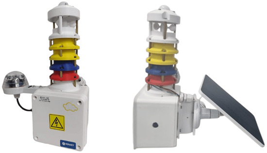
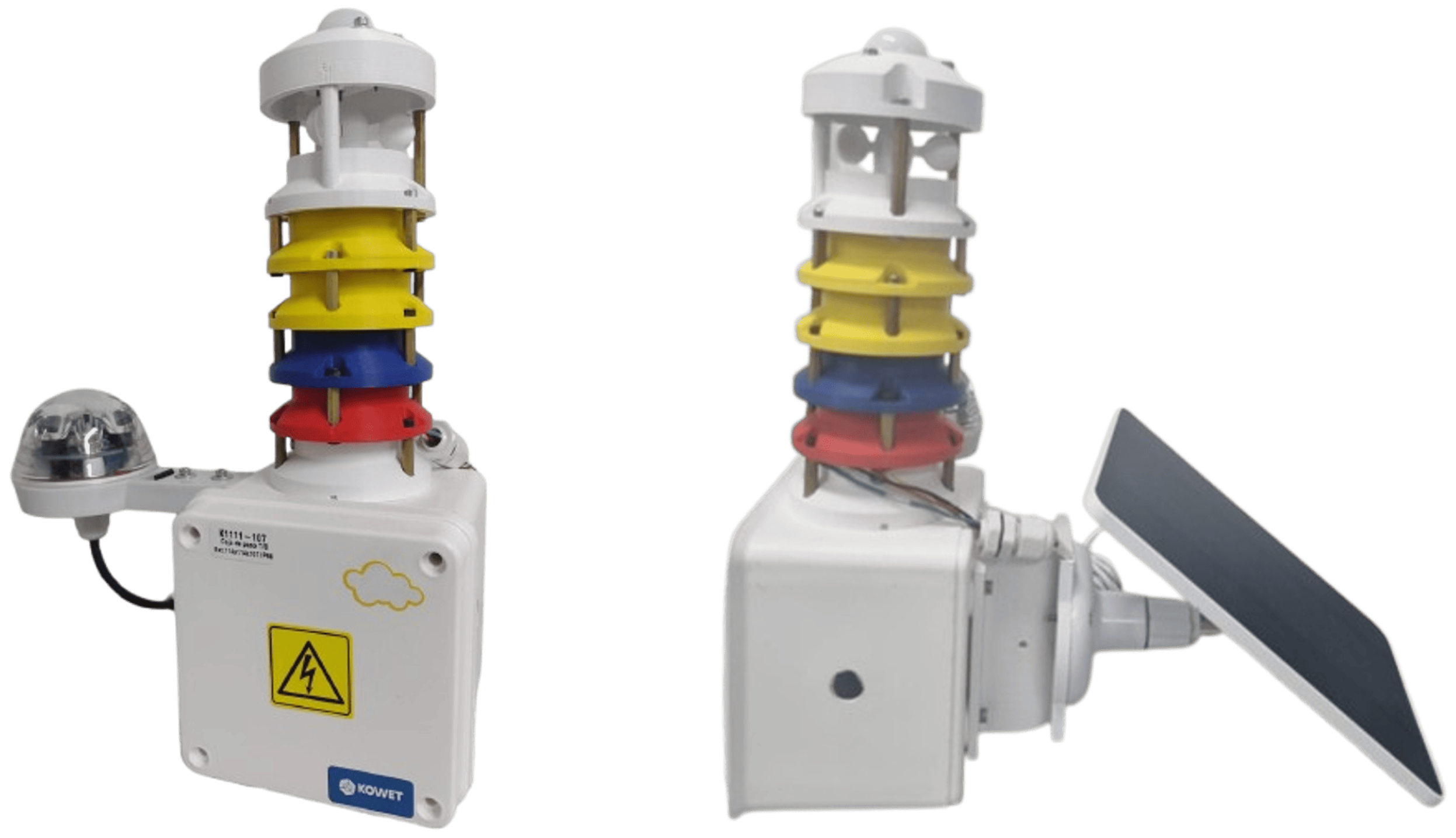
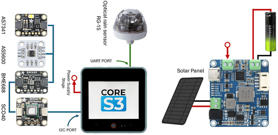
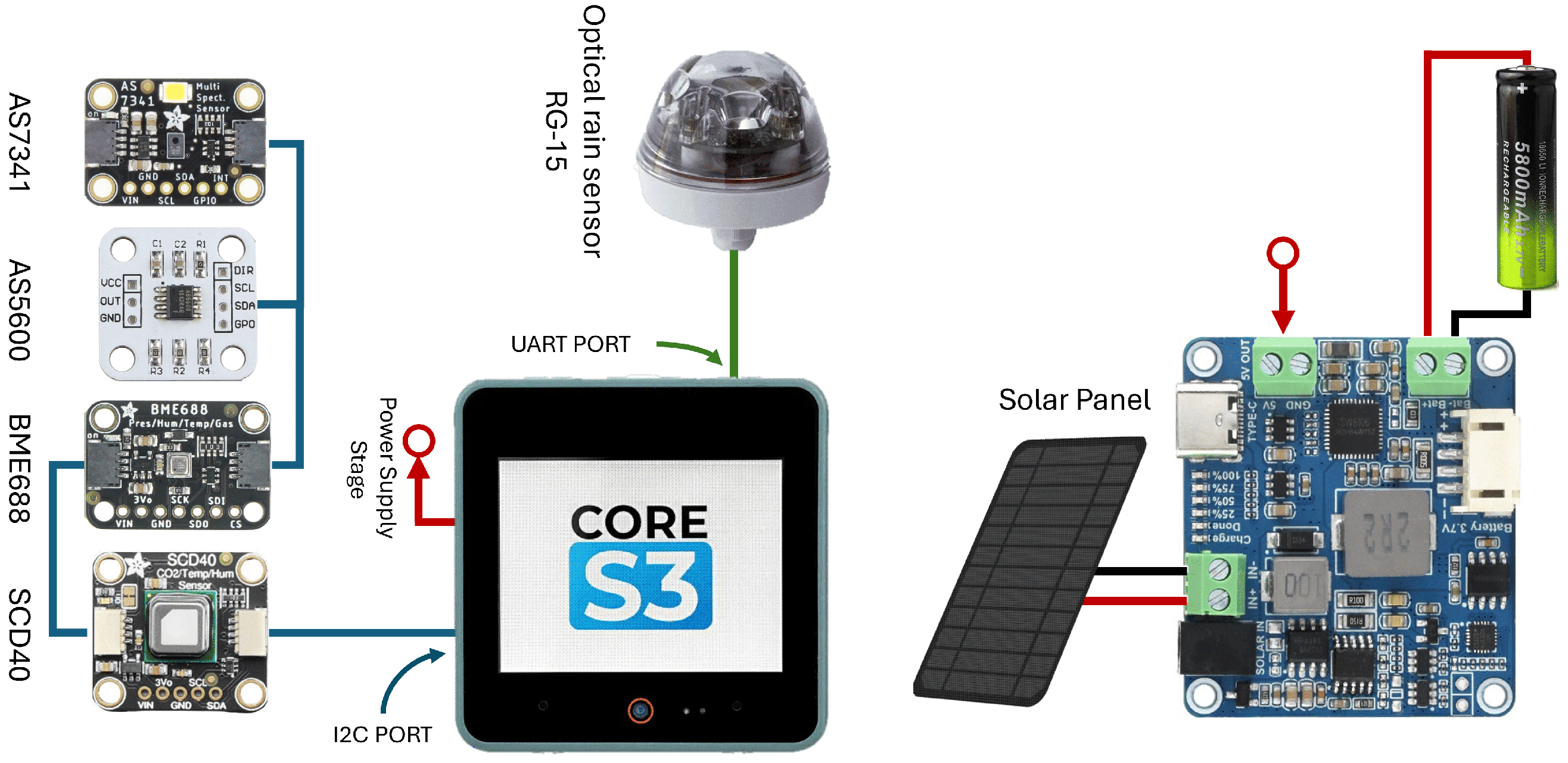
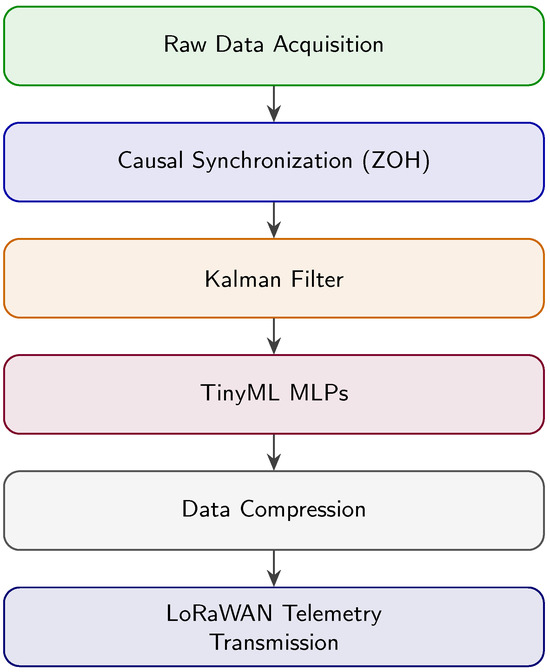
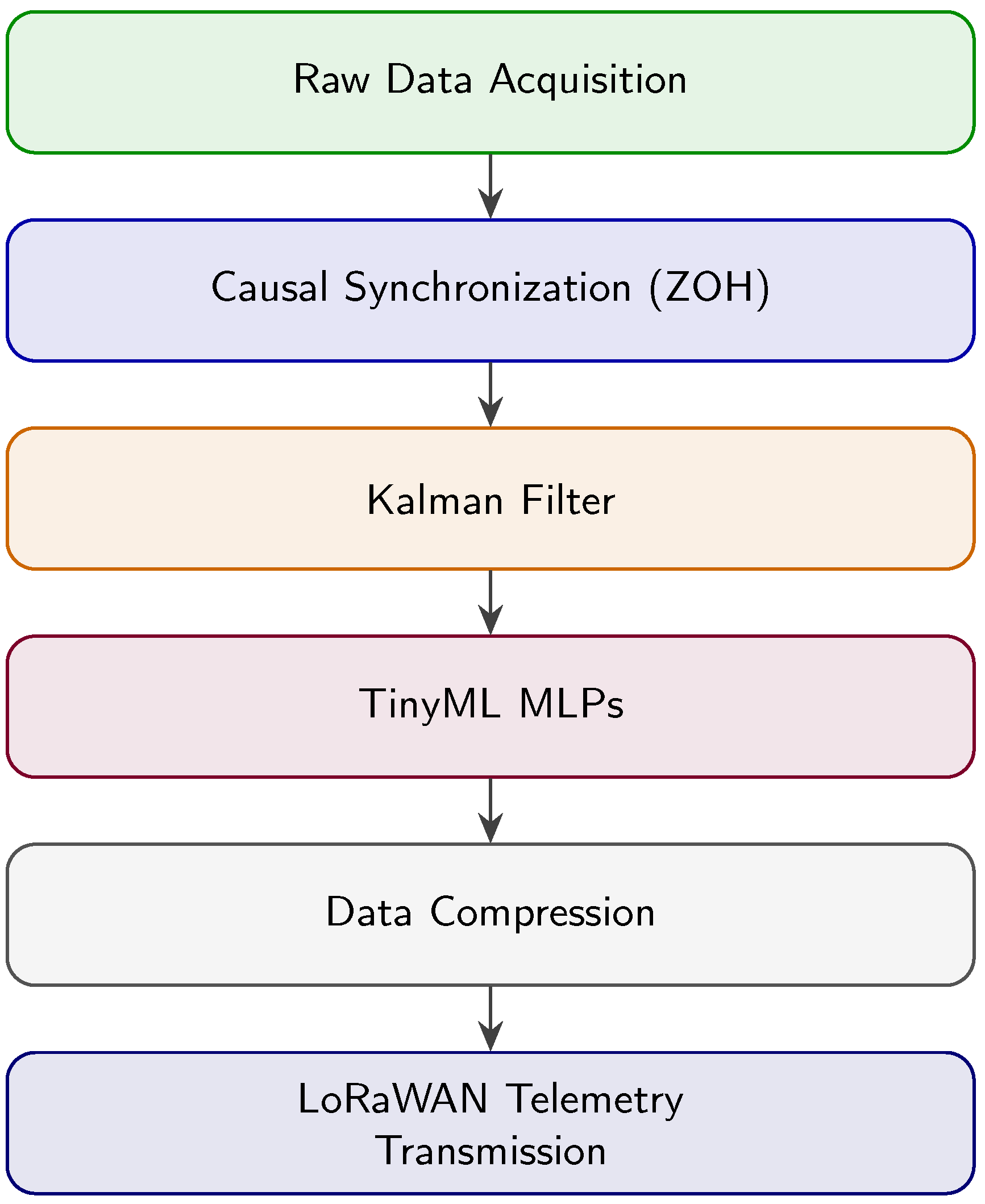
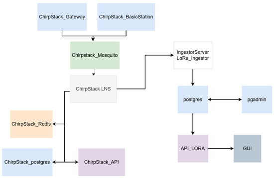
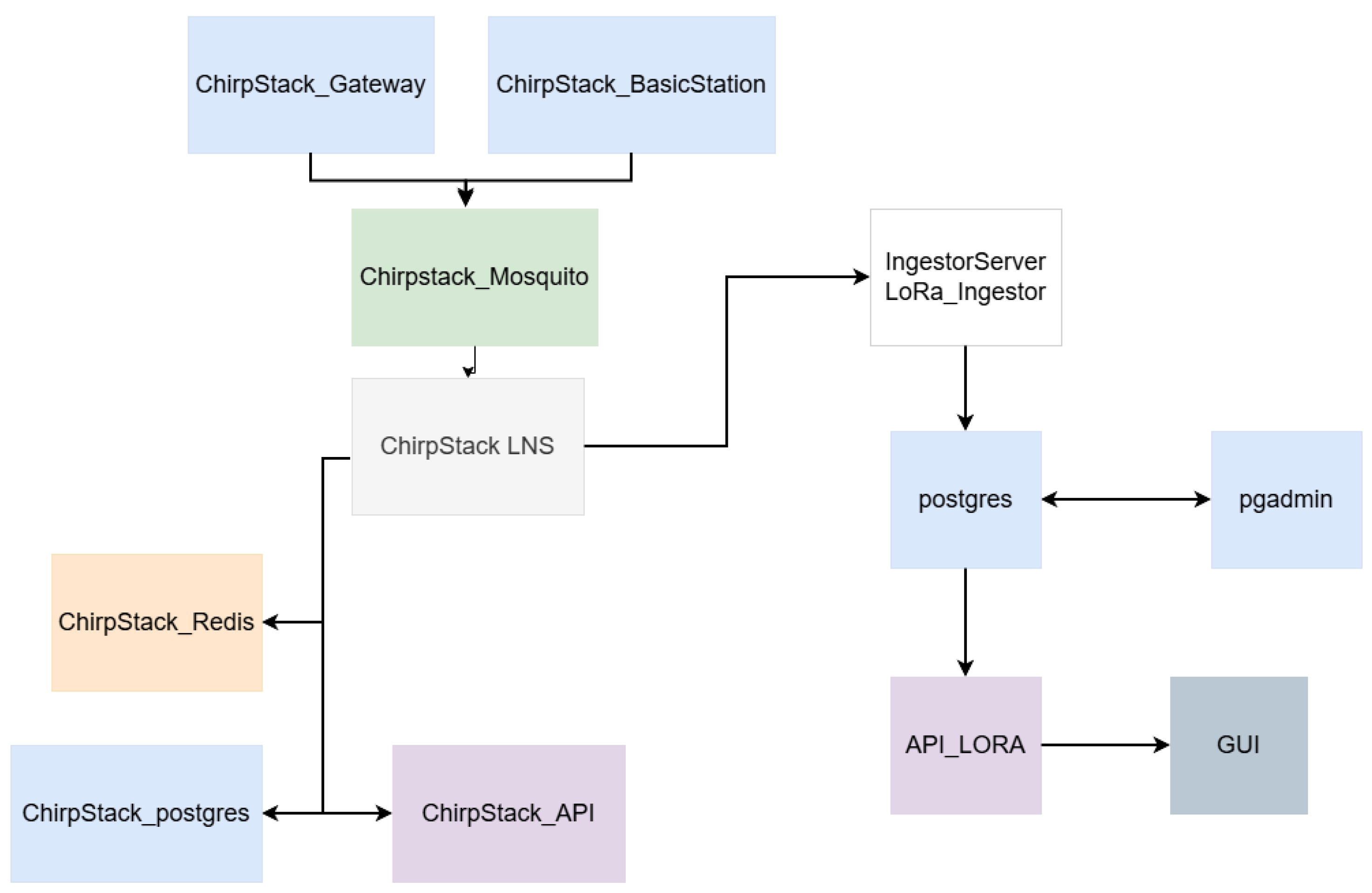
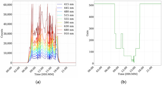
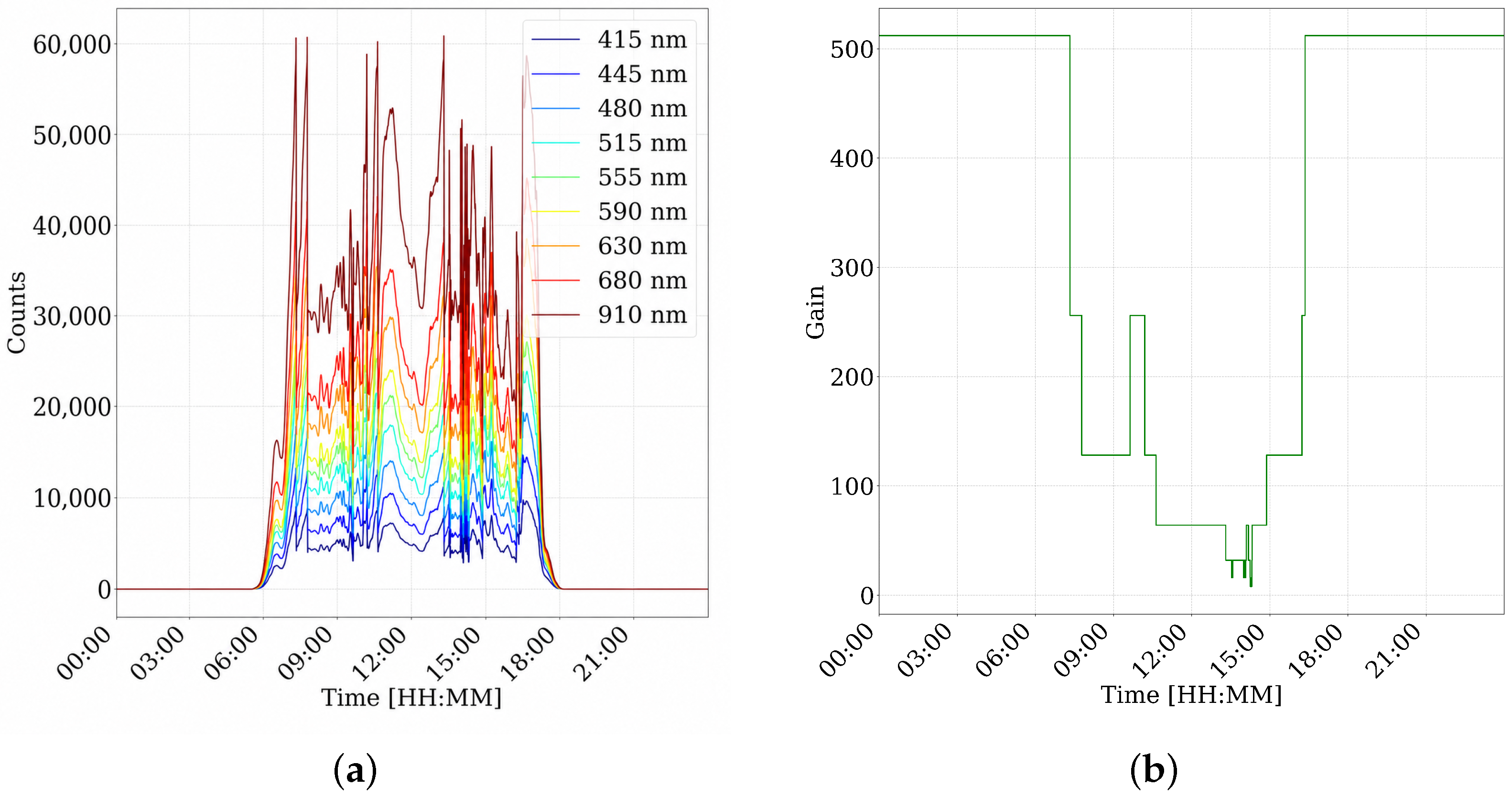
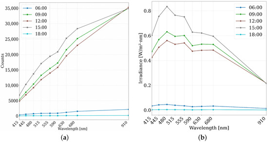
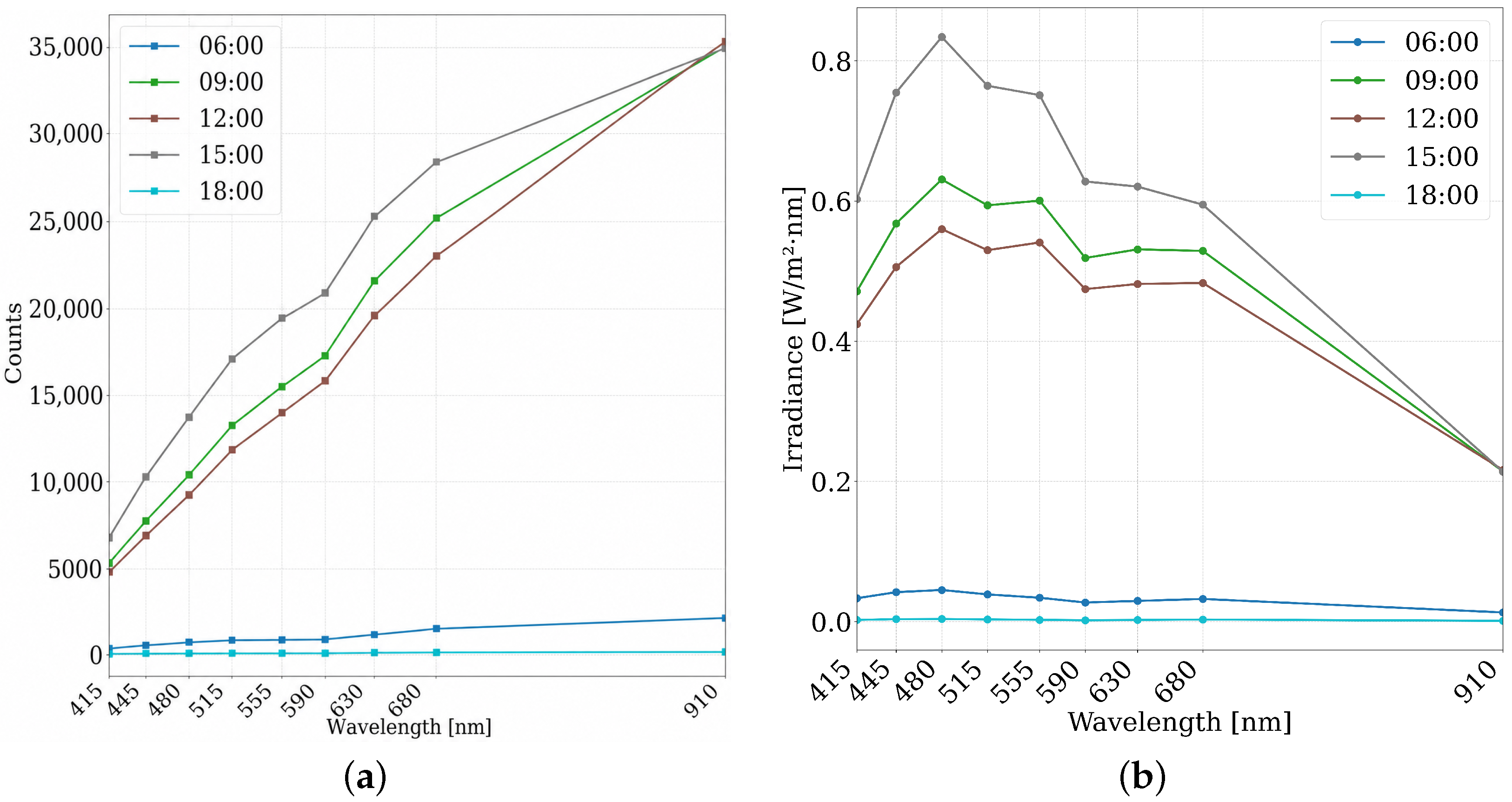
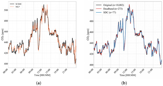
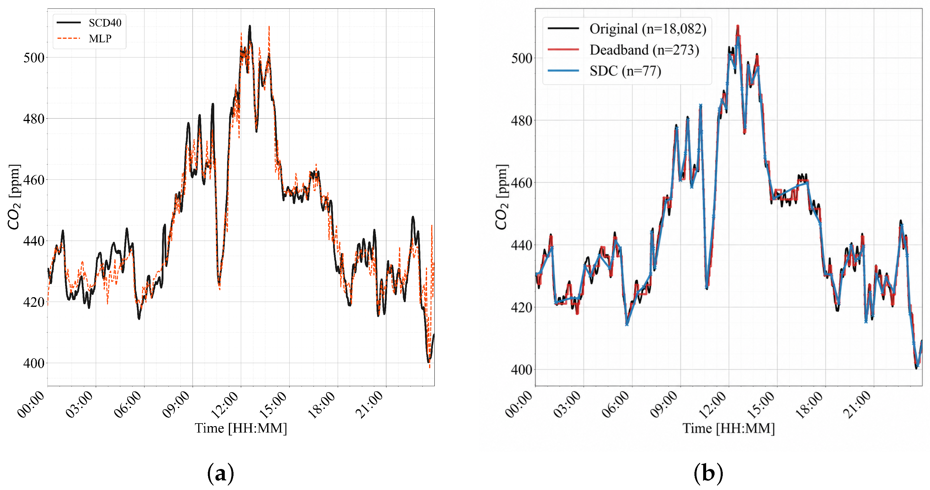
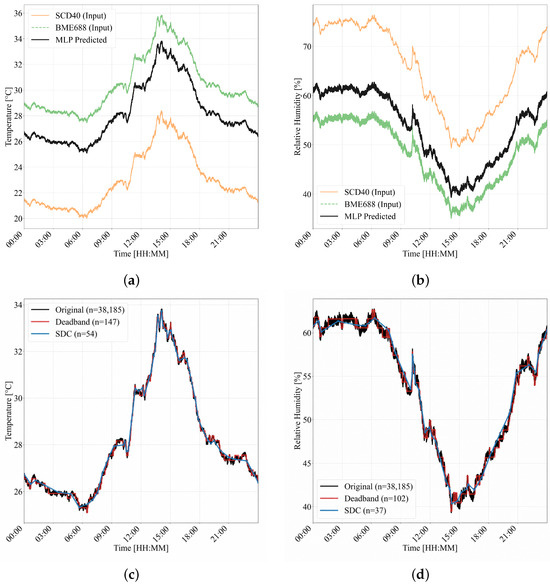
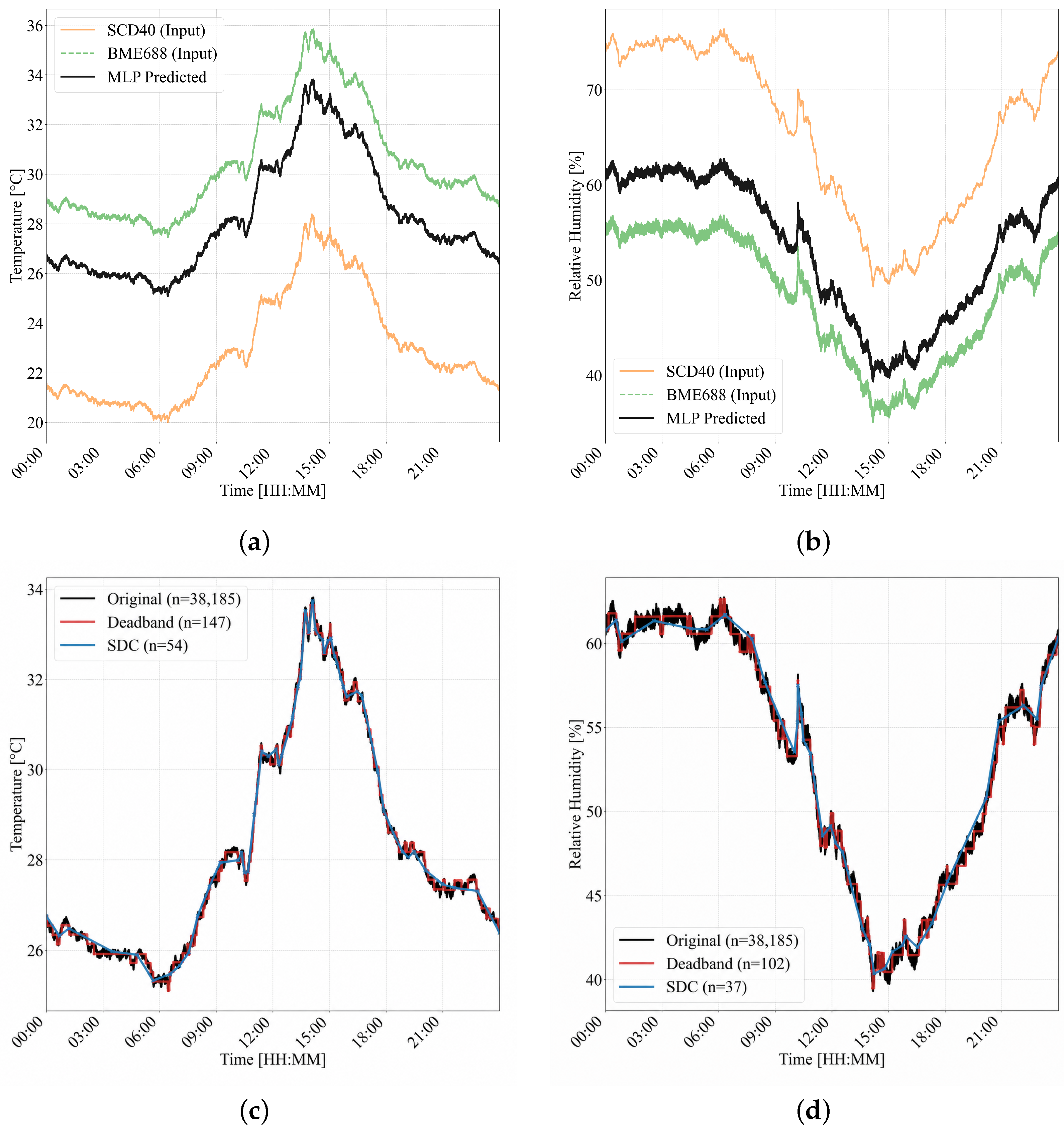
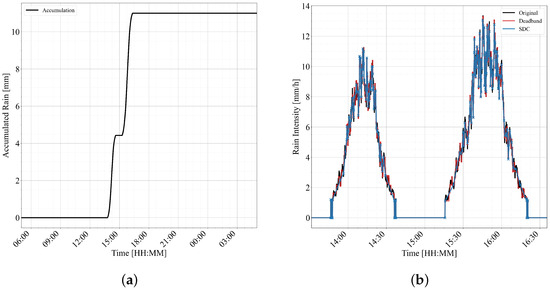
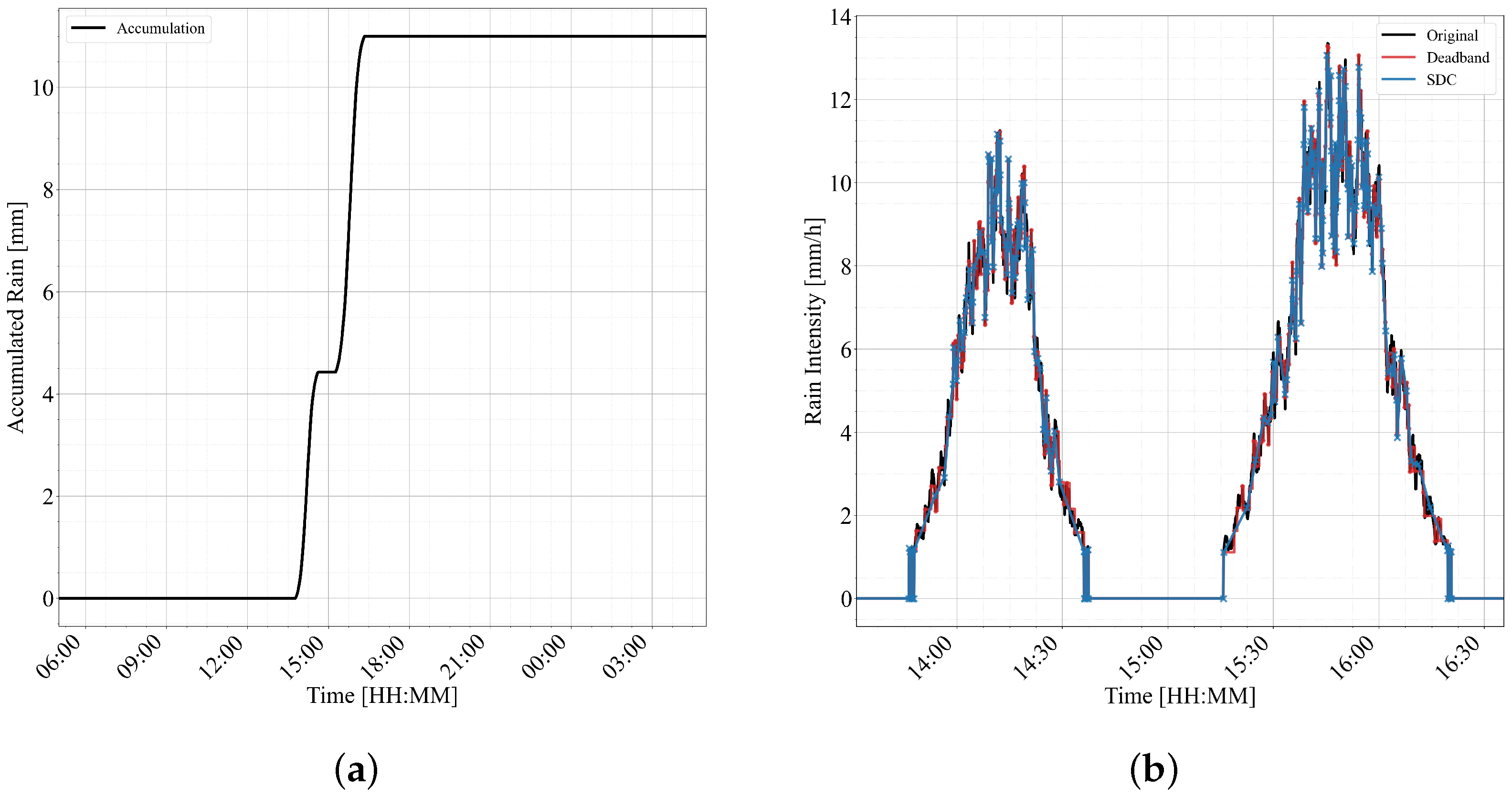
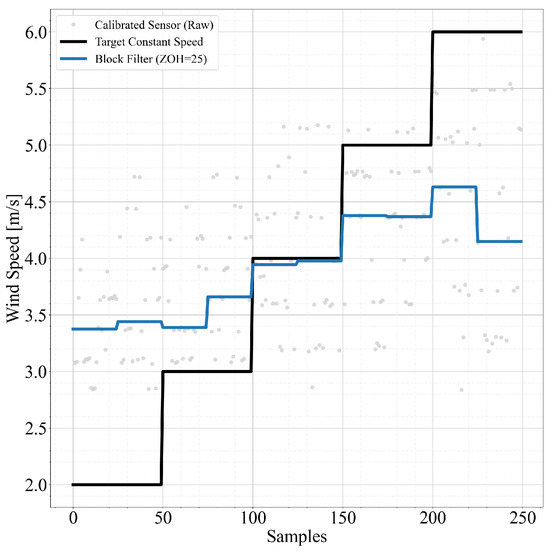
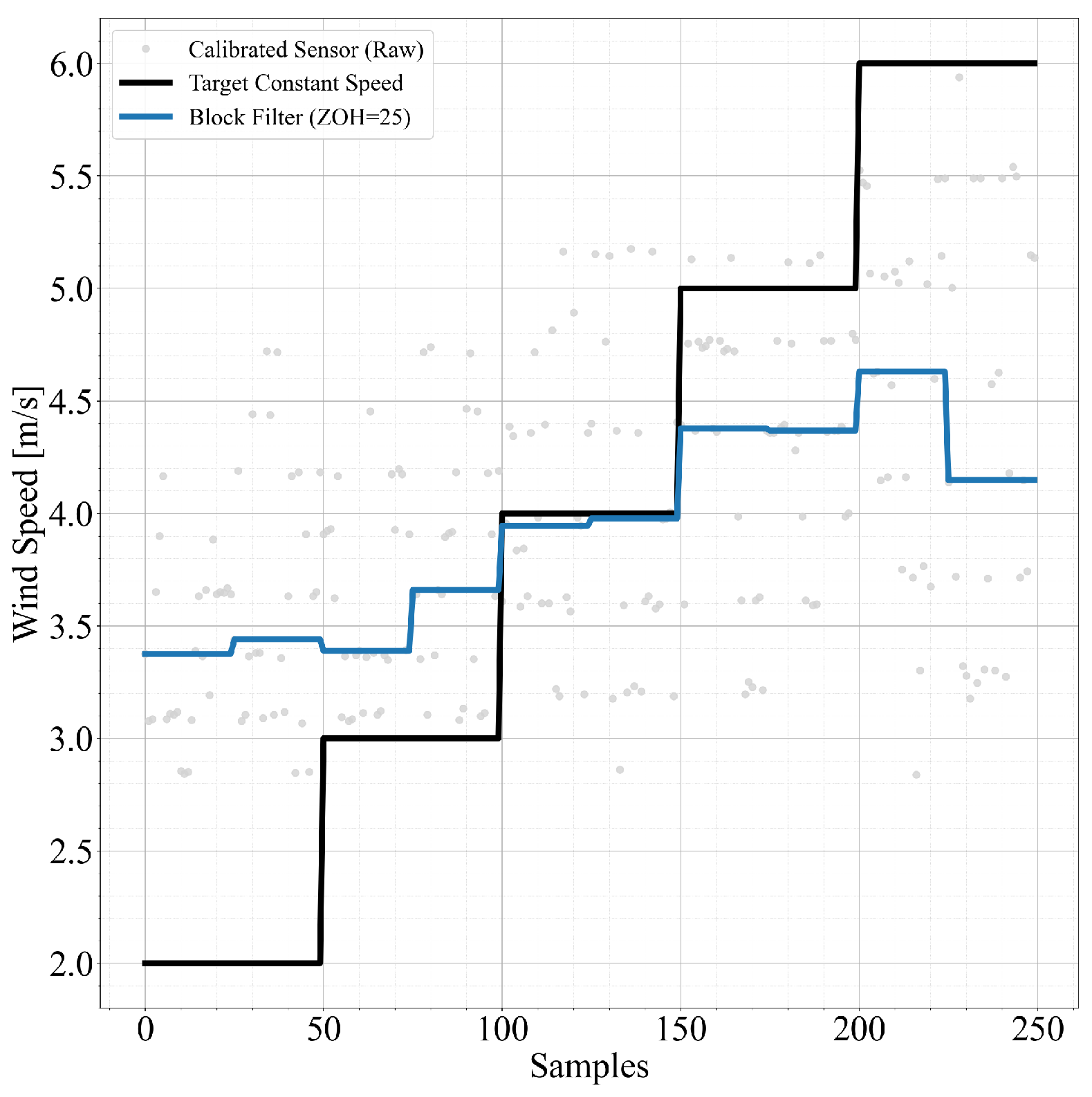

Disclaimer/Publisher’s Note: The statements, opinions and data contained in all publications are solely those of the individual author(s) and contributor(s) and not of MDPI and/or the editor(s). MDPI and/or the editor(s) disclaim responsibility for any injury to people or property resulting from any ideas, methods, instructions or products referred to in the content. |
© 2026 by the authors. Published by MDPI on behalf of the International Institute of Knowledge Innovation and Invention. Licensee MDPI, Basel, Switzerland. This article is an open access article distributed under the terms and conditions of the Creative Commons Attribution (CC BY) license.