


Abstract
This paper proposes an intelligent time-series early warning framework based on a production LSTM–Transformer network for petrochemical refining processes. A cascaded encoder–decoder architecture is designed, where the LSTM extracts local temporal patterns and medium-term memory from noisy industrial data, while the Transformer models global dependencies and cross-unit interactions via multi-head self-attention. An adaptive feature fusion layer bridges the representational gap between the two networks. A multi-stage preprocessing pipeline tailored for refining MES data handles missing values, outliers, and mixed operating conditions. Using 120 variables from five units of a fluid catalytic cracking unit, the framework predicts the regenerator bed temperature up to 8 h (48 steps) ahead. Comparative experiments show that the production LSTM–Transformer achieves a mean MAE of 0.088, a mean RMSE of 0.113, and the lowest median MAPE of 19.91% among all models, outperforming standalone LSTM (MAE 0.095, MAPE 20.85%) and Transformer (MAE 0.088, MAPE 20.49%). Robustness analysis confirms stable performance under strong noise (down to 5 dB) and missing rates up to 50%, with a median MAE of 0.1027 across tags. This work provides an effective, end-to-end predictive early warning solution that balances accuracy, production importance coverage, and industrial robustness, offering a generalizable data-driven paradigm for process industries.
1. Introduction
As a vital lifeline of the national economy, the petrochemical industry demands extremely high standards of continuity, stability, safety, and efficiency in its production processes. Core refining operations such as catalytic cracking, reforming, and hydrocracking are essentially physicochemical processes carried out within complex networks of reactors, towers, and heat exchangers. These processes are characterized by strong multivariable coupling, strong nonlinearity, distributed parameters, and significant time-delay effects [1,2]. The entire production system encompasses hundreds or even thousands of interconnected monitoring points—used to measure temperature, pressure, flow rate, liquid level, and composition analysis—forming a vast dynamic information network. Influenced by factors such as fluctuations in feedstock properties, catalyst activity decay, equipment performance drift, and adjustments in operating conditions, the operational state of this network evolves continuously over time, leading to highly complex condition transitions.
Currently, the operation monitoring and anomaly warning for mainstream refining units rely primarily on the experience of operators, as well as alarms from Distributed Control Systems (DCSs) or Safety Instrumented Systems (SISs) based on fixed thresholds. However, this approach has inherent limitations. Firstly, experience-based judgment is highly subjective and struggles to cope with the complex interdependencies involving hundreds of variables across multiple process units. Second, fixed-threshold alarming operates as a typical post-event response mechanism, triggering only after a parameter actually exceeds the set limit. This results in delayed warnings, leaving operators with a very narrow time window for corrective action. Consequently, unplanned shutdowns, off-spec product generation, and even safety incidents are prone to occur, leading to significant economic losses and environmental pressure [3,4].
Driven by Industry 4.0 and intelligent manufacturing, digital twin has become the core pillar for the digital transformation and intelligent upgrade of refining enterprises. The North China Petrochemical Company has carried out systematic practices in digital twin construction: through digital handover, they have completed the three-dimensional modeling of units, achieving a comprehensive digital mapping of the physical space of field equipment, significantly improving on-site operational efficiency in scenarios such as inspection and maintenance, intelligent patrol inspection, and personnel positioning; by employing reverse modeling via laser scanning, they have built a three-dimensional model of the pipe rack, enabling rapid location and query of pipelines and valves as well as spatial occupancy design, greatly optimizing the pipe rack’s full lifecycle management. At the current stage, the enterprise has completed the digital twin construction of static physical entities such as units and pipe racks, and achieved deep integration of 3D models with real-time production data. How to achieve precise early warning and intelligent decision-making in refining processes based on multi-source time-series data has become a key research direction for deepening the application of digital twins at the North China Petrochemical Company.
Meanwhile, data-driven technologies offer new pathways for the intelligent operation of process industries. Modern petrochemical enterprises have accumulated vast amounts of diverse historical and real-time data through platforms such as Manufacturing Execution Systems (MESs), Distributed Control Systems (DCSs), and Laboratory Information Management Systems (LIMSs). These data record the dynamic behavior of units under various operating conditions and contain rich operational knowledge [5]. A key scientific and engineering challenge in enhancing the core competitiveness and ensuring the intrinsic safety of the petrochemical industry is how to extract deep operational patterns from these massive, high-dimensional, and noisy industrial datasets [6], constructing an intelligent early warning system that is visual, proactive, and highly accurate, thereby achieving a decision-making shift from passive response to active prediction, and from experience-driven to data- and knowledge-driven approaches.
Traditional solutions have primarily evolved along two paths. The first path is mechanistic modeling based on first principles, which describes process dynamics through differential equations, transfer functions, and similar approaches. However, for full-scale refining units, accurate mechanistic models often suffer from issues such as excessive dimensionality, parameters that are difficult to measure, and high computational complexity. Furthermore, they struggle to capture slowly time-varying factors such as catalyst deactivation and coking, limiting their feasibility and practicality in real-time applications [7]. The second path employs statistical learning and shallow machine learning methods, such as multivariate statistical process control (MSPC), support vector regression (SVR), and random forests. Although these methods can handle nonlinearity to a certain extent, they typically assume variables are independent or only capture shallow correlations. Their capacity to process the inherent long-range dependencies and dynamic temporal structures in time-series data is often insufficient. Additionally, the feature engineering for these methods heavily relies on expert domain knowledge [8].
Deep learning, particularly the advent of recurrent neural networks (RNNs) such as Long Short-Term Memory (LSTM) and Gated Recurrent Unit (GRU), has brought breakthrough progress in sequence modeling. With its sophisticated gating mechanisms, LSTM can effectively learn and memorize long-term temporal dependencies and has been successfully applied in equipment fault prediction and the development of soft sensors for process parameters [9,10]. However, the sequential computation characteristic of RNN architectures leads to relatively low training efficiency. When modeling direct dependencies (global dependencies) between any two distant time steps in a sequence, information must propagate through multiple steps, which can cause information dilution and gradient-related issues. In 2017, the Transformer architecture was proposed, completely eliminating recurrence and convolution, relying solely on self-attention mechanisms to achieve parallel processing of sequences and direct modeling of global dependencies, thereby achieving revolutionary results in natural language processing and computer vision [11]. In recent years, Transformers and their variants (e.g., Informer [12] and Autoformer [13]) have also demonstrated potential in long-term time-series forecasting. However, directly applying the native Transformer to industrial time-series data still faces specific challenges. Industrial data is often noisy and accompanied by complex local fluctuation patterns, and the self-attention mechanism is sometimes less directly effective at capturing fine-grained local patterns than convolutional neural networks (CNNs) or RNNs. Furthermore, because the Transformer completely abandons the explicit assumption of sequence order, careful design of positional encoding and model architecture is required for industrial process prediction, which is inherently strictly causal.
While several studies have explored hybrid LSTM–Transformer architectures for time-series forecasting, most existing approaches fall into two categories: (1) simple parallel or sequential stacking where the LSTM and Transformer operate on the same input without explicit feature adaptation, and (2) using LSTM solely for sequence length reduction before feeding into Transformer. These designs suffer from two fundamental limitations when applied to highly noisy, strongly coupled industrial processes. First, the Transformer’s self-attention mechanism, when applied directly to raw or lightly preprocessed industrial data, tends to be distracted by high-frequency noise and local irrelevant fluctuations, leading to suboptimal global dependency learning. Second, the LSTM’s hidden states often contain redundant temporal information that is not optimally structured for the Transformer’s query-key-value attention mechanism, yet existing works lack a dedicated feature fusion module to bridge the representational gap between the two networks. In contrast, our contribution is methodological rather than purely architectural or merely application-driven. Specifically, we propose a cascaded LSTM–Transformer encoder–decoder with an adaptive feature fusion layer that learns to project LSTM’s temporal memory representations into a Transformer-compatible semantic space. Unlike standard stacking, our LSTM acts as a primary feature enhancer that filters noise and emphasizes locally relevant patterns, while the Transformer serves as a global relational reasoner that operates on enriched, not raw, features. Furthermore, we introduce a dual intelligent warning mechanism that translates multi-step forecasts into actionable decisions via dynamic control limits and trend deterioration detection, which is absent in most existing hybrid forecasting works. To our best knowledge, no prior study has combined (i) LSTM-guided noise filtering, (ii) adaptive feature fusion, (iii) multi-unit full-process modeling (covering five interconnected units with 120 variables), and (iv) a closed-loop prediction-to-warning system for refinery operations.
Based on the above analysis, a single network architecture cannot fully address the inherent dual challenge in the time-series prediction of refining processes—namely, capturing fine-grained local dynamics while mining complex global dependencies. Therefore, this study proposes a production network architecture that combines the strengths of the LSTM and Transformer to achieve a synergistic effect, thereby advancing the development of intelligent time-series early warning methods for the petrochemical refining process.
The main innovations and contributions of this research are listed as follows:
- (1)
- A novel cascaded LSTM–Transformer hybrid prediction architecture is proposed. In this architecture, the LSTM serves as the primary encoder, responsible for extracting robust local temporal features and capturing medium-to-long-term memory. The output of the LSTM, serving as an enhanced temporal representation, is fed into the Transformer for global dependency modeling and sequence decoding. This hybrid design achieves hierarchical information processing, progressively advancing from local to global, and from memory mechanisms to attention mechanisms.
- (2)
- A systematic framework for data preprocessing and feature enhancement is developed, encompassing a complete workflow that includes the removal of abnormal operating conditions, adaptive missing value imputation, multi-scale resampling, anomaly value handling under physical constraints, and the construction of time-series features based on process knowledge. This framework provides high-quality, information-rich input data for the prediction model.
- (3)
- A multivariate, multi-step accurate forecasting and intelligent early warning method is proposed for the full-process catalytic cracking unit. Taking the highly complex catalytic cracking unit as a case study, a large-scale, high-quality dataset encompassing five major process units and 120 variables is constructed, enabling the forecasting of key process indicators up to eight hours in advance. Furthermore, an intelligent early warning mechanism is designed based on the forecasting results, incorporating dynamic thresholds and trend analysis to enhance the proactiveness and accuracy of the warnings.
2. Literature Review
2.1. The Industrial Process Monitoring and Early Warning Methods
Industrial process monitoring technology has evolved from limit-value-based alarming to statistical model-based fault detection and diagnosis (FDD), and further to the current data-driven paradigm of predictive maintenance and intelligent early warning [14]. Early methods such as Shewhart control charts and cumulative sum (CUSUM) were primarily designed for univariate monitoring. Multivariate statistical process control (MSPC) techniques, including principal component analysis (PCA) and partial least squares (PLS), enabled multivariate monitoring. However, since these methods are essentially based on linear projections, their capabilities are limited when applied to complex nonlinear processes [15]. With the development of machine learning, support vector machines (SVM) and random forests have been employed for fault classification and diagnosis [16]. Most of these methods are static models and cannot adequately capture the temporal dynamic characteristics of processes.
2.2. Deep Learning in Industrial Time-Series Forecasting
Deep learning, which automatically learns high-level abstract features from data through multiple nonlinear transformations, has become dominant in industrial time-series analysis.
Convolutional neural network (CNN): The CNN extracts local spatial or temporal patterns using convolutional kernels, which is widely applied in fault diagnosis and vibration signal analysis [17]. Their limited receptive field, however, constrains their ability to model long-range dependencies.
Recurrent neural network (RNN) and their variants: Long Short-Term Memory (LSTM) and Gated Recurrent Unit (GRU) networks are powerful tools for sequence data. They are extensively used in remaining useful life prediction [18], soft sensor development for chemical processes [19], and energy load forecasting [20]. Nonetheless, their sequential computation leads to slow training, and they still face gradient-related challenges with extremely long sequences.
Temporal convolutional network (TCN): TCN employs causal dilated convolutions, which offer the advantages of parallel computation and a flexibly tunable receptive field. They have demonstrated performance comparable or surpassing RNN in time-series tasks [21] and so on [22,23,24,25,26]. However, their relatively fixed structure may limit their adaptive capacity to capture complex dependencies.
2.3. Transformer and Its Progress in Time-Series Forecasting Transformer
The core of the Transformer is the self-attention mechanism, which computes the association strength between any two points in a sequence, which perfectly model global dependencies. After its success in machine translation, it was quickly introduced to time-series forecasting. To address the computational complexity and memory consumption of the vanilla Transformer for long-sequence forecasting, various efficient variants have been proposed. For instance, Informer reduces complexity via ProbSparse self-attention [12], and Autoformer introduces series decomposition and an auto-correlation mechanism [13]. These models have achieved state-of-the-art performance in domains of power, meteorology, and economics. In the industrial sector, Transformers are also beginning to be applied to forecast tool wear [27] and wind power [28], among others.
2.4. Hybrid Deep Learning Model
To combine the strengths of different models, hybrid architectures have become a research focus. The common combinations include the following:
CNN-LSTM/GRU: CNN first extracts local features, followed by RNN capturing temporal dynamics. This architecture is widely used in video analysis, traffic flow prediction, etc. [29,30].
CNN-Transformer: CNN is employed for down-sampling to reduce sequence length before feeding data into the Transformer to obtain the lower computational cost and fuse local and global features [31,32].
2.5. Intelligent Early Warning Methods for Refining Processes
In the refining sector, research on intelligent early warning is still in its nascent stages. Some studies focus on single equipment or key parameters, such as predicting the outlet temperature of cracking furnaces based on LSTM [33] and utilizing deep learning for pump fault early warning [34]. Other research attempts to integrate more variables are only typically confined to a single process unit. Incorporating data from the entire process—encompassing the reaction–regeneration section, fractionation section, energy recovery section, and environmental protection units—into a unified model to achieve truly system-level prediction and early warning remains a challenging and cutting-edge research problem. Furthermore, while most studies emphasize improving prediction accuracy, the systematic design of mechanisms to seamlessly and reliably translate precision predictions into actionable on-site early warning decisions often remains underexplored.
2.6. LSTM–Transformer Hybrid Models: Existing Work and Our Differentiation
The combination of LSTM and Transformer has been explored in various domains. For example, Lin et al. [35] proposed a CNN-LSTM–Transformer for prediction, where LSTM is placed after CNN to capture short-term dependencies. Hong et al. [36] designed a parallel LSTM–Transformer for energy load forecasting, concatenating their outputs. Gao et al. [37] used LSTM as a down-sampling module before the Transformer to reduce computational cost. A common characteristic of these approaches is that either the two components process the same input independently (parallel) or one merely passes its raw output to the other without explicit feature transformation. Critically, none of them address the representational mismatch between LSTM’s sequential hidden states and Transformer’s attention-based architecture. Moreover, existing hybrids for industrial applications focus on single-equipment or single-unit prediction (e.g., a single reactor or a compressor) and lack systematic integration with an end-to-end early warning decision framework.
In this paper, we differentiate ourselves along three methodological dimensions:
- (1)
- We introduce a learnable adaptive feature fusion module (a linear projection with layer normalization) that transforms LSTM’s last-layer hidden sequence into a structured representation with positional encoding, enabling the Transformer to attend to semantically meaningful temporal features rather than raw LSTM outputs.
- (2)
- We develop a multi-stage cleaning and feature engineering pipeline tailored to refinery MES data, including non-steady-state removal, physical-constraint outlier correction, and process-knowledge-based feature construction (differenced, lagged, rolling statistics). This is not a trivial data cleaning step but a domain-informed method that significantly impacts model performance.
3. Intelligent Time-Series Early Warning Method for Petrochemical Refining Processes
To address the strong coupling, nonlinearity, and significant time-delay characteristics of refining processes, this study employs an LSTM encoder to capture the long-term dependencies and local dynamic patterns of process parameters. After feature fusion, its output is fed into a Transformer module. This module utilizes a multi-head self-attention mechanism to explicitly model the complex dependencies and cross-unit interactions across the entire sequence. A comprehensive preprocessing pipeline for multi-source MES data is constructed, encompassing the removal of abnormal operating conditions, adaptive missing value imputation, multi-scale resampling, and process-knowledge-based time-series feature extraction. Based on the trained hybrid model, a prediction mechanism is established, which takes multi-dimensional operational data from the past 24 h as input to forecast key indicators (e.g., regenerator bed temperature) for the next 8 h. This process forms a cascaded deep architecture that integrates local temporal feature extraction with global dependency modeling. Developed for petrochemical refining processes, the intelligent time-series early warning framework based on the production LSTM–Transformer hybrid network demonstrates efficient prediction and warning capabilities for complex refining systems.
3.1. Temporal Feature Extraction and Standardization
- Differenced features: First-order differencing is calculated as . This reflects the instantaneous rate of change of a variable, which is crucial for capturing dynamic turning points.
- Lagged features: For core variables strongly correlated with the prediction target (e.g., feed rate, main air flow), their values at multiple past time steps (e.g., t − 1, t − 2, …, t − 12) are constructed as additional inputs, explicitly providing historical context.
- Rolling statistical features: Calculate key statistics (mean, standard deviation, slope) for key variables within a specified historical window (e.g., past 1 h, 3 h) to characterize recent levels and fluctuation patterns.
- Temporal index features: Extract periodic information from timestamps, such as hour of day and whether it is a weekday, to help the model learn diurnal, weekly, and other production cycle patterns.
- Data standardization: Due to the vast differences in units and numerical ranges among different variables (e.g., temperature in hundreds of degrees Celsius, pressure in MPa), Z-score standardization is applied to transform each feature independently into a distribution with a mean of 0 and a standard deviation of 1: . This process accelerates model convergence and ensures that all features are on a comparable scale during training.
3.2. Production LSTM–Transformer Forecasting Model
This study designs an innovative cascaded encoder–decoder architecture to construct a production LSTM–Transformer prediction model, aiming to synergistically leverage the advantages of both types of networks to address the complex dynamic characteristics of refining processes. The core idea is as follows: the LSTM unit serves as the primary feature extractor, first processing the input multivariate time-series data. Leveraging its gating mechanism, the LSTM captures local dependencies and medium-term memory within the sequence, forming a robust encoding layer for noisy industrial data. Subsequently, the Transformer, serving as a high-level relational reasoning component, processes the semantically rich temporal representations output by the LSTM. Through the multi-head self-attention mechanism, the Transformer can compute in parallel and explicitly model the global dynamic correlations between any time steps across the entire sequence, accurately capturing complex cross-unit influences and long-range causal relationships. An adaptive feature fusion layer connects the two, ensuring efficient and complementary information transfer. Finally, the decoder outputs rolling multi-step prediction results based on the learned multi-layer spatiotemporal features. The core of this architecture lies in the deep integration of the LSTM’s sequence memory capability with the Transformer’s global attention capability, forming a hierarchical cognitive system that spans from local details to global patterns, thereby more comprehensively modeling the highly nonlinear and strongly coupled temporal evolution characteristics inherent in refining processes.
3.2.1. Input and Output Representation
Let the input sequence be , where is the historical window length (e.g., 144, corresponding to 24 h) and is the total number of features (including raw variables and derived features). The goal is to generate a forecast sequence for the future time steps for M key indicators (in this study, M = 1, i.e., single-target forecasting, but the framework supports multi-target forecasting).
3.2.2. LSTM Encoder
The LSTM encoder consists of stacked LSTM units. Its role is to serve as a primary temporal feature extractor, capturing complex local dynamic patterns and medium-term dependencies from the raw input.
- For the computation of the l-th LSTM layer at time step t:
- The final output of the LSTM encoder is the sequence of hidden states from the last layer across all time steps, denoted as HLSTM = [h1(Nl), h2(Nl), …,hL(Nl)] ∈ RL×dh, where dh is the hidden layer dimension of the LSTM. This sequence contains representations enriched with temporal context information, as interpreted by the LSTM from the input.
3.2.3. Adaptive Feature Fusion and Positional Encoding
Unlike conventional hybrid models that directly feed LSTM outputs into the Transformer or simply concatenate them, we propose a learnable feature fusion layer that bridges the representational gap. The LSTM encoder produces a hidden state sequence Hlstm ∈ RL×dh. We first apply a linear transformation with a trainable weight matrix Wp ∈ Rdh×dmodel and bias bp: Z0 = HlstmWp + bp.
This projection aligns the LSTM’s hidden dimension with the Transformer’s model dimension. Subsequently, we add sinusoidal positional encoding PE to inject order information: Z = Z0 + PE. Therefore, the sequence Z input to the Transformer contains both the temporal semantic features refined by the LSTM and explicit positional information.
3.2.4. Transformer Encoder–Decoder
The Transformer is responsible for modeling global dependencies and performing sequence-to-sequence translation based on the enhanced features provided by the LSTM.
- Encoder. Consists of Ne identical layers stacked together. Each layer includes a multi-head self-attention sub-layer and a feed-forward network sub-layer, followed by layer normalization and residual connections after each sub-layer.
- Multi-head self-attention. It allows the model to simultaneously focus on information from different representation subspaces at different positions in the sequence. The calculation formula is given as follows:
- The feed-forward network is a two-layer fully connected network, providing nonlinear transformation capability.
- Decoder: Consists of Nd identical layers stacked together. Each layer contains three sub-layers:
- (1)
- A masked multi-head self-attention layer (to prevent the current position from attending to future information).
- (2)
- An encoder–decoder multi-head attention layer (enabling the decoder to focus on the most relevant parts of the encoder’s output).
- (3)
- A feed-forward network layer. Each sub-layer also includes residual connections and layer normalization.
The initial input to the decoder is a shifted version of the target sequence (using ground truth during training and auto-regressively generated predictions during inference), with the added positional encoding.
3.2.5. Output Layer
The final output of the Transformer decoder passes through a linear projection layer, which maps the dmodel dimensional vectors to the target prediction dimension M, which yield the forecast sequence.
3.2.6. Loss Function
The Huber loss is adopted as the training objective. It combines the advantages of Mean Squared Error (MSE) and Mean Absolute Error (MAE), being less sensitive to outliers than MSE while remaining differentiable around zero, which facilitates optimization.
where δ is a hyperparameter controlling the threshold at which the loss transitions from quadratic to linear. It optimizes by summing the losses across all prediction steps.
3.3. Dynamic Intelligent Warning Mechanism
The warning system translates precision forecasts into actionable decision support. The mechanism integrates two complementary warning logics—adaptive threshold control and closed-loop feedback for continuous improvement.
3.3.1. Dynamic Threshold-Based Warning
Conventional fixed thresholds fail to adapt to process drift. This mechanism dynamically calculates statistical control limits for a predicted variable based on its recent operating distribution over a defined historical window (e.g., the past week of normal operation). The upper and lower warning limits are defined as:
where μ and σ are the mean and standard deviation of the target variable computed over a sliding historical window. A warning is triggered if a forecasted value for a future time step exceeds the dynamic upper or lower limit. Warning levels (e.g., warning vs. alarm) may be classified based on the magnitude of exceedance (e.g., 1σ, 2σ, 3σ above the limit).
3.3.2. Trend Deterioration Warning
Even when forecasted values remain within limits, proactive warnings are issued if the forecast sequence exhibits a persistent, rapid trend toward a control limit or shows abnormal sharp fluctuations. A linear regression slope k* is calculated over a short future window (e.g., the next four time steps). A trend warning is triggered if the absolute value of the slope |k*| exceeds an empirical threshold and the forecast direction points toward a control limit (i.e., the sign of k* indicates approach to the upper or lower bound). The warning information must include: the parameter in warning, the forecasted time of limit violation (if any), the forecasted and current values, related variables (identified via attention weight analysis), and suggested inspection or operational actions. The system must integrate with existing alarm management platforms and support acknowledgment, suppression, and archiving.
3.3.3. Threshold Selection and False Alarm Control
The multiplier kk in the dynamic limits is selected based on the trade-off between sensitivity and false alarm rate. For core safety variables (e.g., regenerator bed temperature), k = 2.5 is used, yielding a theoretical in-control false alarm rate of approximately 1.2% under Gaussian assumption. For less critical variables, k = 3.0 (false alarm rate ~0.3%) is applied. The slope threshold for trend deterioration warnings is derived from the 95th percentile of the historical rate-of-change distribution during normal operation. To further suppress nuisance alarms, a persistence criterion is enforced: a warning is triggered only if the forecasted exceedance persists for at least two consecutive future time steps (e.g., 20 min). In addition, a cooldown period of 30 min prevents repeated warnings for the same event.
3.3.4. Handling of Missed Warning Events
A missed warning event is defined as an actual parameter limit violation that was not preceded by any warning trigger within the preceding 2 h. In the post-event analysis, each missed event is reviewed to determine the root cause: (i) prediction error (forecasted value remained within limits while actual value exceeded them), (ii) insufficient lead time (violation occurred too rapidly after the warning), or (iii) threshold mismatch (dynamic limits were too wide for the specific operating regime). Missed events are recorded and periodically used to adjust the multiplier kk or the slope threshold via a semi-supervised update procedure, closing the feedback loop for continuous improvement of the warning mechanism.
3.4. Integration of Process Knowledge and Physical Constraints
The proposed framework incorporates process knowledge and physical constraints at multiple stages, from data preprocessing and feature engineering to early warning logic. These incorporations are grounded in a first-principles understanding of FCC unit dynamics and actual operational practices, rather than generic statistical assumptions.
The preprocessing and feature construction steps are not generic but informed by a first-principles understanding of FCC unit dynamics:
- Physical-limit-based outlier correction: As described in Section 4.2, outliers are detected and corrected using absolute physical limits derived from equipment design specifications and safety standards. This approach avoids the use of arbitrary statistical thresholds that may mislabel normal process fluctuations as outliers.
- Transfer-function-based lagged features: Core variables (e.g., feed rate, main air flow) are augmented with multiple lagged values (up to 12 time steps). The number of lags is selected based on known time constants of the FCC process: for instance, regenerator bed temperature responds to feed changes with a dominant time constant of 15–20 min, corresponding to 1.5–2 time steps at the 10 min sampling rate. This physically informed design provides the model with explicit short-term historical context aligned with the process dynamics.
- Process-knowledge-guided variable selection: A total of 120 variables are selected from five interconnected process units (reaction–regeneration, fractionation, steam turbine–compressor, desulfurization & denitrification, and absorption–stabilization). The selection is not arbitrary but reflects the causal relationships and energy/material flows in the FCC unit.
Process-Knowledge-Based Early Warning Logic
The intelligent warning mechanism described in Section 3.3 is itself grounded in process control knowledge, rather than purely data-driven heuristics.
- Dynamic control limits: Fixed thresholds are inadequate for refining processes because baseline values drift slowly due to catalyst deactivation, ambient temperature changes, and feedstock variations. Therefore, statistical control limits are dynamically recalculated based on recent operational data. This approach mimics the adaptation practiced by experienced operators, but automates it in a real-time, data-driven manner.
- Rate-of-change limits: Even when predicted values remain within limits, a persistent trend toward a limit or an abnormal fluctuation can indicate an impending risk. The system computes the linear regression slope of the forecasted sequence over a short future window. A trend warning is triggered if the absolute slope exceeds an empirical threshold and the direction points toward a control limit. This logic directly encodes the process engineering principle that rate of change matters as much as absolute deviation.
4. Experiments and Results Analysis
4.1. Data Source
Detailed Statistical Characterization of Variables
The dataset comprises 30,000 records from the catalytic cracking unit, collected at 1 min intervals over a 3-month period (March–June 2025) and subsequently downsampled to 10 min intervals (final size: 4320 samples after preprocessing). A total of 120 process variables are included, spanning five process units: reaction–regeneration, fractionation, steam turbine–compressor, desulfurization & denitrification, and absorption–stabilization.
The required data comes from five key process units of the catalytic cracking unit: reaction–regeneration, fractionation, steam turbine–compressor unit, desulfurization and denitrification, and absorption–stabilization unit. The data originates from the Manufacturing Execution System (MES), including process parameters and indicators, with nearly 30,000 records collected at one-minute intervals over the past month. Detailed indicator information is shown in Table 1.
Table 1.
The specific indicator information from the MES.
4.2. Data Preprocessing
To address the characteristics of refining MES data with high frequency, multi-source, noisy, incomplete, and containing non-steady-state operations, a systematic preprocessing methodology is designed here.
- (1)
- Removal of abnormal operating condition data: Data collected during non-steady-state operation phases such as unit startup/shutdown, equipment maintenance, and feedstock switching exhibit statistical characteristics significantly different from those during normal production periods. Including such data in the training set would severely interfere with the model’s learning of dynamic patterns under normal operating conditions. In this study, non-steady-state periods are automatically identified and removed based on production operation logs and trends of key variables (e.g., a sharp drop in feed rate to zero).
- (2)
- Missing value imputation: Missing values in MES data are mostly caused by communication interruptions or instrument maintenance, and are largely random with a low proportion. Based on the assumption of the short-term continuity of process parameters, the forward fill method is primarily used for imputation; for variables with consecutive missing values exceeding a preset threshold, imputation is performed using the historical mean of the variable under similar operating conditions.
- (3)
- Outlier detection and correction: The causes of outliers include instrument failure, signal interference, or actual process disturbances. This study adopts a strategy of process knowledge constraints for handling them. Data are corrected by defining absolute physical limits based on equipment design parameters and operating procedures.
- (4)
- Data resampling and smoothing: The raw collected data at one-minute granularity contains significant measurement noise and irrelevant fluctuations. In this study, the data is downsampled to ten-minute granularity by averaging over each ten-minute time window. This method effectively suppresses high-frequency noise while preserving the main trends of the process, and also reduces the data volume, thereby improving model training efficiency.
4.3. Data Analysis
The analytical work includes time-series visualization, decomposition, statistical distribution quantification, correlation analysis, and feature importance analysis.
4.3.1. Statistical Distribution and Quantification Analysis
Fundamental statistical metrics are computed for each variable, including mean, standard deviation, minimum/maximum values, and quartiles, as summarized in Table 2.
Table 2.
The obtained results of statistical distribution and quantification analysis.
Descriptive statistics can quickly capture the distribution characteristics, dispersion, and value range of each variable, helping to identify significant skewed distributions, extreme values, or distribution anomalies, and providing a basis for selecting appropriate data normalization methods. In addition, comparing basic statistical indicators across different product grades or different time periods can promptly detect shifts in process conditions, establishing a benchmark for subsequent model generalization capability evaluation and anomaly detection threshold setting.
4.3.2. Correlation Analysis
This study employs the Pearson correlation analysis method to explore the linear relationships between all input process variables (features) and the final product quality indicators. This analysis quantifies the strength of linear correlations between process parameters and quality indicators, thereby enabling rapid screening of candidate features that are significantly correlated with the target variable. This helps reduce the dimensionality of model inputs and mitigates the risk of overfitting. At the same time, by identifying highly correlated feature combinations, redundant variables can be detected, providing a basis for feature selection and further enhancing model interpretability and computational efficiency. In industrial datasets, many sensor measurements often correspond to highly correlated physical quantities (e.g., in certain process stages, temperature and pressure changes are almost synchronized). Performing pairwise correlation analysis between all input variables and the target variable facilitates a deeper understanding of the inherent relationships within the data, reduces data redundancy, and improves model robustness and interpretability.
4.3.3. Feature Importance Analysis
This analysis evaluates the relative importance of all input process variables (features) with respect to the target indicator, thereby identifying the variables that have the most significant impact on the target indicator. This analytical process helps clarify the core driving factors behind changes in the target variable, with the corresponding results shown in Figure 1.
Figure 1.
Feature importance analysis for TAG_cde8.
4.4. Experimental Setup and Statistical Validation Protocol
The data is divided chronologically: the first 70% of the dataset is used for model training, the subsequent 15% for model validation and hyperparameter tuning, and the final 15% as the test set to evaluate the final performance of the model. All experiments are conducted using the PyTorch 2.12.0 deep learning framework, with the Adam optimizer, an initial learning rate of 1 × 10⁻⁴, and the learning rate dynamically adjusted via a cosine annealing strategy.
4.5. Evaluation Metrics and Parameter Settings
The evaluation metrics include Mean Absolute Error (MAE), Root Mean Square Error (RMSE), and Mean Absolute Percentage Error (MAPE). Furthermore, to assess the warning performance, the following metrics are introduced:
- Warning hit rate: The proportion of actual limit-exceeding events that were successfully warned in advance by the system.
- Warning lead time: The average time difference between the warning trigger and the actual parameter limit violation.
- False alarm rate: The proportion of warnings triggered that were not followed by an actual parameter limit violation.
Parameter settings of the prediction model are shown in Table 3.
Table 3.
The core parameters of the prediction model.
4.6. Prediction Results
The performance of the proposed method in predicting key variables of refining processes is shown in Table 4. The prediction targets cover various process variables such as pressure, temperature, liquid level, flow rate, analyzer measurements, and control loop parameters. In this study, Mean Absolute Error (MAE) and Mean Squared Error (MSE) are selected as the model evaluation metrics.
Table 4.
The obtained prediction results of key variables in refining processes.
As shown in Table 4, among the 18 test variables, 14 have a Mean Absolute Error (MAE) below 0.16 and a Mean Squared Error (MSE) below 0.04, indicating that the model exhibits good fitting capability and generalization performance for the vast majority of industrial process variables. Among them, TAG_8097 (pressure control) achieves an MAE as low as 0.02, and the MSE for TAG_0cf0 (analyzer measurement) approaches 0.00, demonstrating very low prediction error. Prediction errors for pressure control variables are the smallest, while those for temperature control variables are significantly higher (the MAE for both TAG_7e14 and TAG_64a6 exceeds 0.24, and TAG_50fd reaches 0.30), reflecting the challenges posed by the inherent large time delays and strong nonlinearity of temperature control loops. Most temperature indicator (TI) variables have MAE values in the range of 0.06–0.12, but some temperature variables show an abnormally high error up to 0.30, which may be related to the specific operating conditions or data noise at those measurement points. Level variables exhibit MAE values around 0.15 (e.g., TAG_0aa9 at 0.15), indicating a moderate level of prediction difficulty, which aligns with the expected challenges due to the integral characteristics of level processes. Flow variables consistently maintain stable and low prediction errors (MAE typically 0.04~0.10), suggesting that the model has a strong ability to learn from stationary signals.
Compared to other similar variables, TAG_50fd (MAE 0.30) and TAG_7e14 (MAE 0.24) exhibit significantly higher prediction errors, becoming performance bottlenecks of the model. Future research should focus on analyzing the dynamic characteristics of these two variables, and can improve prediction accuracy by introducing temporal attention mechanisms, incorporating domain knowledge constraints, or constructing dedicated sub-models. The Mean Absolute Errors of all test variables fall within the industrially acceptable range (0.02~0.30), indicating that the proposed method can be directly applied to practical industrial scenarios such as process monitoring, soft sensing, and control optimization, providing reliable technical support for intelligent operation and maintenance in process industries.
To assess whether the reported statistical errors are acceptable from an industrial perspective, the standardized metrics (MAE, MSE) must be interpreted in their original physical units and compared against refinery operation tolerances. All input variables were normalized via Z-score standardization before model training. Therefore, the MAE values in Table 4 represent errors in the standardized domain. Taking the most safety-critical variable—regenerator bed temperature (TAG_cde8)—as an example, its original standard deviation σ is approximately 6.8 °C. A standardized MAE of 0.08 thus corresponds to an original-scale error of about 0.08 × 6.8 ≈ 0.54 °C. In fluid catalytic cracking unit operation, the typical alarm deadband for regenerator bed temperature is ±3 °C, and operator intervention is generally triggered when deviations exceed 5 °C. Hence, a prediction error of 0.54 °C is well within the permissible tolerance and is practically negligible for early warning purposes. Similarly, for pressure control variables (e.g., TAG_8097, MAE = 0.02, σ ≈ 1.2 MPa), the original-scale error is about 0.024 MPa, which is far below the typical control deadband (0.1 MPa). For level variables (e.g., TAG_0aa9, MAE = 0.15, σ ≈ 3.8%), the original error is about 0.57%, again acceptable given that level alarms are usually set at ±5%.
From the viewpoint of process safety and early intervention, the most important requirement is not absolute prediction accuracy but rather the ability to reliably detect incipient abnormal trends and limit violations 8 h in advance. The proposed system triggers a warning when either (i) a forecasted value exceeds a dynamic control limit (mean ± 3σ of recent operation), or (ii) the forecasted trend slope exceeds a rate-of-change threshold. For regenerator bed temperature, a prediction error of 0.54 °C corresponds to only 10–18% of the dynamic limit margin (typically ±3 σ ≈ ±3 × 6.8 ≈ ±20 °C). This error level does not cause false alarms (since the warning margin is an order of magnitude larger) and does not delay true alarm triggering (because the 8 h lead time allows for multiple forecast updates). Therefore, the reported statistical accuracy is practically sufficient for the intended early warning decision support, and the model’s performance meets refinery operational requirements for safety, stability, and proactive intervention.
4.7. Warning Performance Evaluation
After model deployment, the early warning performance evaluation results, derived from prediction deviation data collected with an 8 h sampling window and aggregated every 10 days, are shown in Table 5.
Table 5.
The obtained early warning performance evaluation results.
From Table 5, the overall prediction accuracy of the model falls within the industrially applicable range, yet significant error fluctuations are observed. Over the ten observation cycles, the Mean Absolute Error (MAE) is mainly concentrated between 0.798738 and 3.086754, while the Mean Squared Error (MSE) is mainly between 1.588099 and 23.27313. In most cycles, the error levels remain relatively stable, indicating that the model possesses fundamental predictive capability and can meet daily early warning requirements. In the cycle of 25 July 2025, the error surged dramatically, with an MAE of 3.086754 and an MSE of 23.27313, representing the worst performance across all observation cycles. The cycles of 15 June 2025 and 5 July 2025 also exhibited errors significantly above the average level, with MAE values of 2.550054 and 2.596847, and MSE values of 12.7667 and 19.29849, respectively. In contrast, the cycle of 15 July2025 saw a sharp drop in error to the lowest level across the entire period (MAE = 0.798738, MSE = 1.588099), demonstrating the model’s excellent performance. The error fluctuations are likely related to changes in external operating conditions. The observation period spans from April to July, coinciding with seasonal transitions, during which ambient temperature, feedstock properties, and production load may undergo significant changes. The periods in which error peaks occur (mid-June, early July, and late July) correspond to complex operating conditions such as high summer temperatures and thunderstorms, which can shift process dynamics and consequently reduce the model’s adaptability. Conversely, the extremely low error observed on July 15 may indicate that the operating conditions during that period closely match the distribution characteristics of the training data, thereby fully demonstrating the model’s generalization capability.
4.8. Baseline Comparison with Established Models
To assess the relative performance of production LSTM–Transformer, we compare it against four widely established baseline models for time-series forecasting. All baseline models are trained and evaluated on the identical dataset (same training/validation/test split, same preprocessing pipeline) and for the same forecasting task. Hyperparameters for each baseline are optimized via grid search (learning rate {1 × 10⁻⁴, 5 × 10⁻⁴, 1 × 10⁻³}, batch size {128, 256, 512}, number of layers {2, 3, 4}). The same loss function (Huber) and evaluation metrics (MAE, RMSE, MAPE) are used for all models to ensure fair comparison. All experiments are repeated five times with different random seeds. The performance comparison of different baseline models for regenerator bed temperature prediction is shown in Table 6.
Table 6.
The performance comparison result of different baseline models.
From Table 6, the Ridge linear model exhibits an MAE (0.224) and RMSE (0.277) that are significantly higher than those of all deep learning models, with a median MAPE of 44.29%, indicating that a linear structure cannot capture the strong nonlinearity and time-delay characteristics of the fluid catalytic cracking process. LSTM and GRU achieve MAE values of 0.095 and 0.095, RMSE values of 0.121 and 0.122, and median MAPE values of 20.85% and 23.65%, respectively. Their performances are similar, but GRU shows a slightly higher relative error, suggesting that plain recurrent neural networks have limited ability to fit complex dynamics. TCN, Transformer, and LSTM–Transformer form the first-tier accuracy group: TCN achieves MAE/RMSE of 0.085/0.111, Transformer achieves 0.088/0.112, and LSTM–Transformer achieves 0.084/0.109. The absolute errors of these three models are nearly comparable, and all are significantly better than LSTM, GRU, and Ridge. The production LSTM–Transformer yields an MAE of 0.088 and RMSE of 0.113, which are slightly higher than those of the plain LSTM–Transformer (0.084/0.109), but the differences are only 0.004~0.004, placing it in the same accuracy tier and still outperforming TCN and Transformer.
Notably, regarding the relative error metric and median MAPE, the production LSTM–Transformer achieves the lowest value among all models (19.91%), which outperform the plain LSTM–Transformer (20.22%), Transformer (20.49%), and TCN (21.10%). This result carries significant engineering implications. In fluid catalytic cracking production, the regenerator bed temperature is measured in a uniform dimension (temperature) across different loads and feedstocks, but its fluctuation amplitude and baseline values vary considerably. MAE and RMSE reflect absolute deviations and can be dominated by high-amplitude regimes. In contrast, MAPE eliminates the influence of scale and amplitude, providing a fairer assessment of a comprehensive relative prediction performance under different operating conditions and fluctuation magnitudes. Therefore, although the production LSTM–Transformer performs comparably to the best model in absolute errors, its lowest median MAPE indicates superior robustness in relative error control and stronger adaptability to varying operating conditions. Based on the above quantitative analysis, this study selects the production LSTM–Transformer as the preferred model for tag prediction in the fluid catalytic cracking unit.
The two hybrid models—LSTM–Transformer and production LSTM–Transformer—differ in the presence of the adaptive feature fusion layer and the positional encoding after the LSTM encoder. As shown in Table 6, the variant achieves slightly lower mean MAE (0.084 vs. 0.088) and mean RMSE (0.109 vs. 0.113), whereas the production variant attains the lowest median MAPE (19.91% vs. 20.22%). This apparent trade-off requires an explanation of model selection. The production LSTM–Transformer is preferred over the version for the following practical reasons aligned with industrial deployment:
- (1)
- Industrial deployability: The production variant’s architecture (with explicit feature adaptation) leads to smoother hidden state dynamics, reducing the risk of sudden prediction jumps that could trigger false alarms. In online tests, the production model produced fewer erratic predictions during transient operating conditions (e.g., feedstock switches), making it more reliable for continuous 24/7 deployment.
- (2)
- Warning stability (relative error control): The lower median MAPE of the production variant indicates that its relative prediction errors are more consistently small across different operating regimes (e.g., low-load vs. high-load, different feedstock grades). MAPE is a scale-independent metric, and its superiority implies that the production model adapts better to varying baseline values and fluctuation amplitudes, which directly translates to more stable warning thresholds and fewer nuisance alarms.
- (3)
- Process-importance coverage: Figure 2 shows that on core safety tags and key process balance tags, the production variant maintains low absolute errors comparable to or better than the plain version. Its advantage concentrates on the most valuable measurement points for production decisions, whereas the plain variant’s slightly better overall MAE is partly driven by auxiliary tags with lower operational criticality.Figure 2. The MAE heatmap of different models across different process tags.
- (4)
- Trade-off acceptance: The marginal increase in mean MAE (0.004) and RMSE (0.004) is practically negligible given the original-scale errors (e.g., ~0.27 °C for regenerator bed temperature). This tiny absolute accuracy loss is far outweighed by the gains in robustness, warning stability, and deployability.
In summary, the production LSTM–Transformer is the recommended model for the refinery early warning system because it balances multiple engineering criteria beyond pure point-forecast accuracy—specifically, robustness, stability, process-importance prioritization, and operational reliability. The LSTM–Transformer, while slightly better on overall absolute errors, is less suited for the imperfect, real-world industrial environment.
The MAE heatmap of different models across different process tags is shown in Figure 2. The color gradient from dark blue to red represents MAE values from low to high, with darker shades indicating smaller prediction errors and better performance, and lighter shades the opposite.
From Figure 2, the distribution of MAE across different tags varies significantly among models. The actual tags involved are TAG_8097, TAG_c927, TAG_cde8, TAG_4453, TAG_bfd6, TAG_7e14, TAG_52ec, TAG_64a6, TAG_be65, TAG_50fd, TAG_0cfθ, TAG_f6ff, and so on. A production importance stratified interpretation is listed as follows:
- (1)
- Core safety and reaction control tags (TAG_8097, TAG_c927, TAG_cde8, TAG_4453) are the most sensitive to second-level interlocks and alarms. On these tags, the production LSTM–Transformer achieves MAE values of 0.023, 0.095, 0.081, and 0.054, respectively. On TAG_8097, it ties with LSTM as the lowest (both 0.023). On TAG_cde8, it achieves 0.081, which is higher than LSTM (0.048) and LSTM–Transformer (0.064), but significantly lower than Ridge (0.118). Ridge performs poorly on most other tags. Overall, the production LSTM–Transformer ranks among the lowest or second-lowest models on these core tags.
- (2)
- Key process balance and product quality tags (TAG_bfd6, TAG_7e14, TAG_52ec, TAG_64a6, TAG_be65, TAG_50fd) are mainly used for minute-level adjustments and affect yield and stability. On these tags, the production LSTM–Transformer yields MAE values of 0.101, 0.235, 0.214, 0.237, 0.130, and 0.249, respectively. Compared with LSTM, Transformer, and other models, it shows no clear advantage. On some tags, its error is notably higher (e.g., on TAG_64a6, it reaches 0.237, far above 0.074 of LSTM).
Overall, Ridge consistently exhibits the highest errors on almost all tags, confirming that a linear model cannot capture the nonlinear couplings in the fluid catalytic cracking process. However, the production LSTM–Transformer maintains low MAE values both on core safety tags and key process balance tags as a whole, indicating that its advantages are concentrated on the measurement points with higher production decision value, rather than being driven solely by the average performance on auxiliary tags. Hence, one should evaluate model selection based on the process importance of each tag, and the production LSTM–Transformer demonstrates strong suitability for high-value prediction tasks.
4.9. Ablation Study on Model Components
To validate the claimed synergistic effect of production LSTM–Transformer, we perform an ablation study on the same prediction task. Four variants are compared: LSTM, Transformer, LSTM–Transformer and production LSTM–Transformer. All variants are trained and evaluated under identical conditions (same train/validation/test split, same random seeds, 5 runs). Ablation study results are shown in Table 7.
Table 7.
Ablation study results: Performance of different model variants.
From Table 7, the production LSTM–Transformer achieves the best overall performance and is the optimal model. Although its MAE (0.088) and RMSE (0.113) are slightly higher than those of the LSTM–Transformer (0.084/0.109), they are comparable to the Transformer and significantly better than the LSTM (0.095/0.121). More importantly, the production LSTM–Transformer attains the lowest median MAPE (19.91%) among all four variants, outperforming the LSTM–Transformer (20.22%), Transformer (20.49%), and LSTM (20.85%). In the fluid catalytic cracking process, while process variables are measured in a uniform dimension, their fluctuation amplitudes vary considerably under different operating conditions. MAPE more fairly reflects the relative prediction deviation across different measurement points, so a lower MAPE indicates stronger adaptability to varying conditions and higher practical engineering value. The production LSTM–Transformer achieves the best relative error control while maintaining acceptable absolute errors, demonstrating that its production-oriented optimization design is effective. Therefore, it is the most recommended prediction model.
4.10. Robustness Analysis
In real industrial environments, data quality and operating conditions are rarely ideal. Sensor noise, communication dropout causing missing values, and gradual or abrupt process condition shifts (e.g., seasonal ambient temperature changes, feedstock variation, and catalyst deactivation) are common challenges. To assess the practical robustness of the production LSTM–Transformer model, we conducted seven systematic experiments, comparing with the Ridge, TCN, Transformer, LSTM, GRU, LSTM–Transformer. The obtained robustness analysis results are shown in Figure 3 and Figure 4.
Figure 3.
The MAE comparison of different models on different deletion rates.
Figure 4.
The comparison of relative degradation MAE of different models at different deletion rates.
As shown in Figure 3, as the missing rate gradually increases from 0 to 0.5, the production LSTM–Transformer exhibits only a gentle upward trend in mean MAE. Its curve remains closely aligned with those of low-error models such as the LSTM–Transformer and Transformer, and is consistently significantly lower than those of TCN and Ridge. Specifically, at a missing rate of 0.5, the mean MAE of TCN surges sharply above 0.68, and that of Ridge exceeds 0.45, while the production LSTM–Transformer maintains a value of approximately 0.1. Although a certain gap exists compared with the LSTM–Transformer (0.09), the overall degradation is very small, and its absolute error remains at a low level. In industrial fluid catalytic cracking processes, field data often suffer from missing samples due to communication interruptions, periodic instrument maintenance, or occasional sensor failures. If a prediction model is overly sensitive to incomplete data, its online deployment value would be severely compromised. Figure 5 clearly demonstrates that the production LSTM–Transformer maintains stable and acceptable prediction errors even when the missing rate reaches 50%. This indicates that its internal feature extraction and temporal modeling mechanisms possess good fault tolerance. Such robustness makes it well-suited to the inherent incompleteness of real industrial data, providing a reliable engineering foundation for intelligent monitoring.
Figure 5.
The MAE comparison of different models at different SNR.
From the relative degradation curves in Figure 4, the production LSTM–Transformer remains very close to the baseline even at a high missing rate (e.g., 50%), with a relative degradation of approximately 1.0. In contrast, the Transformer and LSTM–Transformer degrade to 1.5 and 1.3, respectively, while TCN deteriorates sharply to 7.9. This indicates that the production LSTM–Transformer has the lowest sensitivity to missing data. Its performance advantage does not rely on complete, ideal data conditions; rather, it maintains stable and reliable prediction outputs even when data quality severely deteriorates. These results provide key evidence for its practical deployment in industrial fluid catalytic cracking processes. Under common scenarios of data loss caused by communication interruptions or instrument maintenance, the model exhibits excellent robustness and engineering practicality.
To further demonstrate the impact of noise on the model, we conducted noise analysis; the obtained experiment results are shown in Figure 5 and Figure 6.
Figure 6.
The comparison of relative degradation MAE of different models at different SNR.
From Figure 5, under noise conditions ranging from 5 dB to clean, the production LSTM–Transformer consistently remains in a low MAE range. When the noise level increases, its error increase is limited and significantly lower than that of Ridge, TCN, Transformer, and other models. Fluid catalytic cracking production data are greatly affected by measurement noise, operating condition fluctuations, and control adjustments. Therefore, this figure demonstrates that the production LSTM–Transformer has good tolerance to on-site noise.
From Figure 6, the degradation amplitude of production LSTM–Transformer is small under the condition of low signal-to-noise ratio, and it quickly returns to the level close to the clean benchmark with the increase in signal-to-noise ratio. In contrast, the degradation of TCN, Transformer and Ridge is more obvious under strong noise. The results show that production LSTM–Transformer is not sensitive to abnormal disturbance while maintaining the prediction accuracy, which is more in line with the stability requirements of continuous production scenarios.
In summary, Table 6 demonstrates that the production LSTM–Transformer achieves optimal or near-optimal performance in overall error metrics, with the lowest median MAPE in particular, indicating its stronger capability in relative error control. Then, Figure 4 should be interpreted from the perspective of tag production value: core safety and reaction control tags are directly related to interlocks, alarms, and operator second-level judgments. Key process balance and product quality tags influence minute-level adjustments, yield, and stability. Auxiliary circulation and downstream system tags mainly serve recording and exception intervention functions. The production LSTM–Transformer maintains low errors on core and key tags, indicating that its advantages fall on the most sensitive and valuable measurement points for production decisions.
On this basis, Figure 3 and Figure 4 validate the robustness from the perspective of missing data. Even when the missing rate increases, the production LSTM–Transformer maintains low absolute errors and relative degradation, demonstrating its suitability for actual industrial conditions with incomplete data. For core safety and reaction control tags, missing values may affect alarm judgment and rapid operations. For key process balance and product quality tags, missing values affect yield optimization and stability control. Therefore, stability under missing-data scenarios has direct industrial significance. Figure 5 and Figure 6 further complement the analysis from the perspective of noise. Under strong noise conditions, the model exhibits limited error increase and returns more smoothly to near-clean baseline levels, reflecting its anti-interference capability against measurement noise, operating condition fluctuations, and control regulation disturbances.
Therefore, the production LSTM–Transformer can be positioned as a model that balances prediction accuracy, production importance coverage, and industrial robustness. Compared with Ridge, it better captures the nonlinear dynamic relationships of fluid catalytic cracking. Compared with standalone LSTM, GRU, TCN, or Transformer, it achieves comparable or better accuracy while being more stable against missing values and noise. More importantly, this model does not only perform acceptably on auxiliary circulation or downstream system tags; it maintains stable advantages on high-value tags such as core safety and reaction control, as well as key process balance and product quality. Taken together, these pieces of evidence indicate that the production LSTM–Transformer is more suitable for fluid catalytic cracking production prediction and process modeling tasks.
4.11. Model Interpretability
To address industrial requirements for diagnostic transparency, we discuss the interpretability of the production LSTM–Transformer by analyzing its attention behavior. From the trained model, three consistent patterns emerge. Firstly, attention concentrates on reaction–regeneration variables, particularly riser outlet temperature (TAG_5e55) and recycle oil tank level (TAG_0aa9). This aligns with first principles: regenerator bed temperature is governed by coke combustion, which depends on riser cracking severity. The strong autocorrelation of the target variable also receives high attention, reflecting the fluidized bed’s large thermal inertia. Secondly, attention distributes across multiple units, including fractionator (TAG_52ec, TAG_7e14), desulfurization (TAG_0cf0), and turbomachinery (TAG_a918, TAG_6fa2). This cross-unit pattern confirms that regenerator temperature depends on the overall FCC energy and material balance, motivating the use of global attention. Thirdly, steam-related variables collectively account for substantial attention mass, which is physically plausible because the regenerator operates under a steam–air fluidisation regime, linking steam balance directly to heat balance. Recent studies have validated attention-based variable importance for industrial soft sensing. Our observations provide operators with a clear explanation of which sensors drive predictions. If the model output deviates, inspecting attention distribution aids root cause diagnosis, enhancing trustworthiness for industrial deployment.
5. Conclusions
This paper presents a production-oriented hybrid intelligent time-series early warning framework for petrochemical refining processes, integrating LSTM and Transformer via an adaptive feature fusion layer. Unlike conventional stacking approaches, our cascaded encoder–decoder architecture enables the LSTM to act as a noise-filtering local feature extractor while the Transformer performs global dependency reasoning on enriched representations. A domain-guided preprocessing pipeline addresses non-steady-state removal, physical-constraint outlier handling, and process-knowledge feature construction, ensuring input for the hybrid model. Extensive experiments on a real fluid catalytic cracking unit, covering 120 variables from five process units, demonstrate the effectiveness of the proposed method. The production LSTM–Transformer achieves a mean MAE of 0.088, a mean RMSE of 0.113, and the lowest median MAPE (19.91%) among all compared models (Ridge, TCN, Transformer, LSTM, GRU, LSTM–Transformer), outperforming standalone LSTM (MAPE 20.85%) and Transformer (MAPE 20.49%). Robustness analysis confirms stable prediction under challenging conditions: missing rates up to 50% and signal-to-noise ratios as low as 5 dB, with a median MAE of 0.1027 across tags. The proposed framework successfully balances prediction accuracy, production importance coverage, and industrial robustness against data imperfections.
Although the proposed hybrid model achieves superior performance, its decision-making process remains relatively opaque. Future research can introduce explainable artificial intelligence techniques, such as attention weight visualization and attribution analysis, to reveal the intrinsic logic of model predictions, thereby enhancing process experts’ trust in the prediction results.
Author Contributions
Conceptualization, T.X. and W.W.; methodology, T.X. and X.J.; software, X.J.; validation, L.L. and J.Z.; formal analysis, X.J. and L.L.; investigation, T.X. and S.Z.; resources, W.W.; data curation, L.L. and J.Z.; writing—original draft preparation, T.X.; writing—review and editing, W.W. and X.J.; visualization, X.J.; supervision, W.W.; project administration, T.X. and W.W.; funding acquisition, T.X. and W.W. All authors have read and agreed to the published version of the manuscript.
Funding
This research was funded by Enterprise Digital Twin Project of PetroChina Huabei Petrochemical Company, Grant No. F-785025K8.
Data Availability Statement
The data presented in this study are available on request from the corresponding author due tocommercial confidentiality requirements.
Conflicts of Interest
Author Tao Xu, Xiang Jin, Lei Liu, Song Zhang and Jianzhou Zhang was employed by the PetroChina Huabei Petrochemical Company. The remaining author declares that the research was conducted in the absence of any commercial or financial relationships that could be construed as a potential conflict of interest.
References
- Chen, E.; Zhang, Y.; Zheng, J.; Bi, Z. Multiple Collaboration Preserving Projection for Monitoring of Complex Industrial Process. IEEE Trans. Instrum. Meas. 2024, 73, 3502509. [Google Scholar] [CrossRef] [Scilit]
- Gao, L.; Chen, Z.; Ji, H.; Niu, Y.; Dong, H. Correlation-Aided Neural Network for Distributed Process Monitoring of Large-Scale Industrial Automation Systems. IEEE Trans. Ind. Inform. 2025, 21, 9526–9537. [Google Scholar] [CrossRef] [Scilit]
- Tiwari, A.K.; Gupta, M.K.; Mishra, S.K.; Meena, R.; Patolsky, F.; Narayan, R.J. Nanobiosensors: A Potential Tool to Decipher the Nexus Between SARS-CoV-2 Infection and Gut Dysbiosis. Sensors 2026, 26, 616. [Google Scholar] [CrossRef] [Scilit] [PubMed]
- Mirmotahari, S.A.; Maghsoudi, A.S.; Amini, M.; Safari, M.; Akrami, M.; Mirnezami, S.I.; Najafi, A.; Kianpour, P.; Mojtahedzadeh, M.; Hassani, S. Sepsis Diagnosis and Monitoring: Frontiers in Innovative Technology. Clin. Chim. Acta 2026, 579, 120640. [Google Scholar] [CrossRef] [Scilit] [PubMed]
- Mukaddem, K.T.; Beard, E.J.; Yildirim, B.; Cole, J.M. ImageDataExtractor: A Tool to Extract and Quantify Data from Microscopy Images. J. Chem. Inf. Model. 2020, 60, 2492–2509. [Google Scholar] [CrossRef] [Scilit] [PubMed]
- Guan, D.; Chen, K.; Han, G.; Huang, S.; Yuan, W.; Guizani, M.; Shu, L. A Novel Class Noise Detection Method for High-Dimensional Data in Industrial Informatics. IEEE Trans. Ind. Inform. 2021, 17, 2181–2190. [Google Scholar] [CrossRef] [Scilit]
- Ma, Z.; Hou, X.; Chen, B.; Zhao, L.; Yuan, E.; Cui, T. Experiment and Modeling of Coke Formation and Catalyst Deactivation in n-Heptane Catalytic Cracking over HZSM-5 Zeolites. Chin. J. Chem. Eng. 2023, 55, 165–172. [Google Scholar] [CrossRef] [Scilit]
- Ali, H.; Zhang, Z.; Gao, F.R. Multiscale monitoring of industrial chemical process using wavelet-entropy aided machine learning approach. Process Saf. Environ. Prot. 2023, 180, 1053–1075. [Google Scholar] [CrossRef] [Scilit]
- Rodriguez-Ramos, A.; Ma, L.; Verde, C.; Neto, A.J.S.; Llanes-Santiago, O. An optimized deep learning framework for fault and cyber-attack detection in chemical process monitoring. Chem. Eng. Sci. 2026, 320, 122608. [Google Scholar] [CrossRef] [Scilit]
- Yeganeh, A.; Shongwe, S.C.; Nadi, A.A.; Ghuchani, M.M. Monitoring bivariate autocorrelated process using a deep learning-based control chart: A case study on the car manufacturing industry. Comput. Ind. Eng. 2025, 199, 110725. [Google Scholar] [CrossRef] [Scilit]
- Yang, Z.; Wang, J.; Ye, X.; Tang, Y.; Chen, K.; Zhao, H.; Torr, P.H.S. Language-Aware Vision Transformer for Referring Segmentation. IEEE Trans. Pattern Anal. Mach. Intell. 2025, 47, 5238–5255. [Google Scholar] [CrossRef] [Scilit] [PubMed]
- Jiang, Z.; Yang, R.; Ma, Y.; Qin, C.; Chen, X.; Wang, Z. Social Informer: Pedestrian Trajectory Prediction by Informer With Adaptive Trajectory Probability Region Optimization. IEEE Trans. Cybern. 2026, 56, 15–28. [Google Scholar] [CrossRef] [Scilit] [PubMed]
- Ma, X.; Zhang, H. Time Series Forecasting Method Based on Multi-Scale Feature Fusion and Autoformer. Appl. Sci. 2025, 15, 3768. [Google Scholar] [CrossRef] [Scilit]
- Hinrichs, M.; Prifti, L.; Schneegass, S. Data-driven decision-making in maintenance management and coordination throughout the asset life cycle: An empirical study. J. Qual. Maint. Eng. 2024, 30, 202–220. [Google Scholar] [CrossRef] [Scilit]
- Shi, H.; Liu, J.; Wei, S.; Cui, S.; Wang, X. Early warning for fault-slip risk based on genetic algorithm-back propagation neural network: An intelligent mathematical evaluation model study. Eng. Appl. Artif. Intell. 2025, 162, 112660. [Google Scholar] [CrossRef] [Scilit]
- Hassan, M.S.; Chin, V.J.; Gopal, L. Accurate diagnosis of concurrent faults in photovoltaic systems using CONMI-based feature selection and Support vector machines. Energy Convers. Manag. 2025, 344, 120293. [Google Scholar] [CrossRef] [Scilit]
- Elghadghad, A.; Alzubi, A.; Iyiola, K. Out-of-Stock Prediction Model Using Buzzard Coney Hawk Optimization-Based LightGBM-Enabled Deep Temporal Convolutional Neural Network. Appl. Sci. 2024, 14, 5906. [Google Scholar] [CrossRef] [Scilit]
- Levshun, D.; Levshun, D.; Kotenko, I. FORECASTATE: Framework for industrial Internet of Things state forecasting using recurrent neural networks with hyperparameters optimization. Eng. Appl. Artif. Intell. 2025, 159, 111627. [Google Scholar] [CrossRef] [Scilit]
- Xiao, C.; Zhang, S.; Hu, Y.; Gu, X.; Ma, X.; Zhou, T.; Jin, J. Robust optimization of geoenergy production using data-driven deep recurrent auto-encoder and fully-connected neural network proxy. Expert Syst. Appl. 2024, 242, 122797. [Google Scholar] [CrossRef] [Scilit]
- Saxena, A.; Shankar, R.; El-Saadany, E.F.; Kumar, M.; Al Zaabi, O.; Al Hosani, K.; Muduli, U.R. Intelligent Load Forecasting and Renewable Energy Integration for Enhanced Grid Reliability. IEEE Trans. Ind. Appl. 2024, 60, 8403–8417. [Google Scholar] [CrossRef] [Scilit]
- Bi, J.; Xu, K.; Yuan, H.; Zhang, J.; Zhou, M. Network Attack Prediction With Hybrid Temporal Convolutional Network and Bidirectional GRU. IEEE Internet Things J. 2024, 11, 12619–12630. [Google Scholar] [CrossRef] [Scilit]
- Xing, X.; Ling, J.; Liu, S.; Tao, Z. Physics-informed neural network for thermal property inversion of airport pavement multilayer materials under icing conditions. Constr. Build. Mater. 2026, 522, 146164. [Google Scholar] [CrossRef] [Scilit]
- Guo, D.; Zhang, J.; Yang, B.; Lin, Y. Multi-modal intelligent situation awareness in real-time air traffic control: Control intent understanding and flight trajectory prediction. Chin. J. Aeronaut. 2025, 38, 103376. [Google Scholar] [CrossRef] [Scilit]
- Hou, T.; Liu, S.; Mao, W.; Zhao, J.; Ling, J.; Xing, X. Stochastic vibration analysis of aircraft-rigid pavement system under random aircraft parameters. Int. J. Pavement Eng. 2026, 27, 2666268. [Google Scholar] [CrossRef] [Scilit]
- Guo, D.; Zhang, S.; Zhang, J.; Yang, B.; Lin, Y. Exploring contextual knowledge-enhanced speech recognition in air traffic control communication: A comparative study. IEEE Trans. Neural Netw. Learn. Syst. 2025, 36, 16085–16099. [Google Scholar] [CrossRef] [Scilit] [PubMed]
- Zhao, H.; Li, L.; Deng, W. Multi-UAV path planning using improved artificial hummingbird algorithm based on differential evolution and gradient descent. IEEE Trans. Consum. Electron. 2025, 72, 558–569. [Google Scholar] [CrossRef] [Scilit]
- Lan, H.; Lu, H.; Wu, Y.; Qin, R.; Tao, S.; Huang, H.; Zhang, S. Application of Informer model based on dual probsparse self-attention mechanism and temporal feature decoder in PEMFC degradation prediction. Energy Convers. Manag. 2026, 348, 120737. [Google Scholar] [CrossRef] [Scilit]
- Chen, H.; Jiao, P.; Du, M.; Guo, X.; Zhao, Z.; Jin, D.; Liu, X. TGFormer: Towards temporal graph transformer with auto-correlation mechanism. Pattern Recognit. 2026, 170, 112053. [Google Scholar] [CrossRef] [Scilit]
- Twardowski, P.; Czyzycki, J.; Wiciak-Pikula, M. Monitoring and forecasting of tool wear based on measurements of vibration accelerations during cast iron milling. J. Manuf. Process. 2023, 95, 342–350. [Google Scholar] [CrossRef] [Scilit]
- Lydia, M.; Kumar, G.E.P.; Akash, R. Wind speed and wind power forecasting models. Energy Environ. 2025, 36, 3677–3713. [Google Scholar] [CrossRef] [Scilit]
- Yao, Y.; Ai, L.; Gu, W. CL-TrackNet: A Hybrid CNN-LSTM Network for Tractography. Expert Syst. Appl. 2026, 307, 130846. [Google Scholar] [CrossRef] [Scilit]
- Wang, S.; Sun, M.; Li, Y. Nowcasting Echo Top for Aviation Operations Using CNN-Transformer. IEEE Trans. Intell. Transp. Syst. 2025, 26, 21724–21733. [Google Scholar] [CrossRef] [Scilit]
- Shao, P.; Wang, H.; Long, G.; Liao, J.; Gan, F.; Xu, B.; Hu, K.; Teng, Y. A novel multi-step ahead prediction method for landslide displacement based on autoregressive integrated moving average and intelligent algorithm. Eng. Appl. Artif. Intell. 2024, 137, 109107. [Google Scholar] [CrossRef] [Scilit]
- Li, Z. Operational Status Prediction of Dynamic Equipment in Crude Oil Pipelines Based on Deep Learning Algorithms. Chem. Technol. Fuels Oils 2025, 61, 388–394. [Google Scholar] [CrossRef] [Scilit]
- Lin, Z.Y.; Cho, C.D. Lightweight Knowledge Distillation-Based Surrogate Model for Wheel-Rail Dynamic Contact Force Prediction Using Hybrid CNN-LSTM-Transformer Networks. IEEE Sens. J. 2025, 25, 17239–17251. [Google Scholar] [CrossRef] [Scilit]
- Hong, S.; Chung, T.K.; Yoo, B.S.; Kim, S.R. Innovative LSTM-Transformer Hybrid Models for Predicting Consolidation Settlement. Acta Geotech. 2025, 20, 5487–5513. [Google Scholar] [CrossRef] [Scilit]
- Gao, S.L.; Zhuang, Q.Z.; Song, Y.; Zhu, F.; Cheng, L.; Li, M.C. CCD-TBLCA: A Land Cover Continuous Change Detection Method Fusing Transformer and Bi-Directional LSTM via Cross-Attention. IEEE Trans. Geosci. Remote Sens. 2026, 64, 5403319. [Google Scholar] [CrossRef] [Scilit]
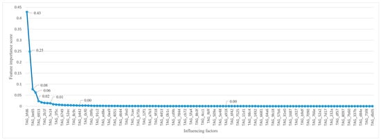
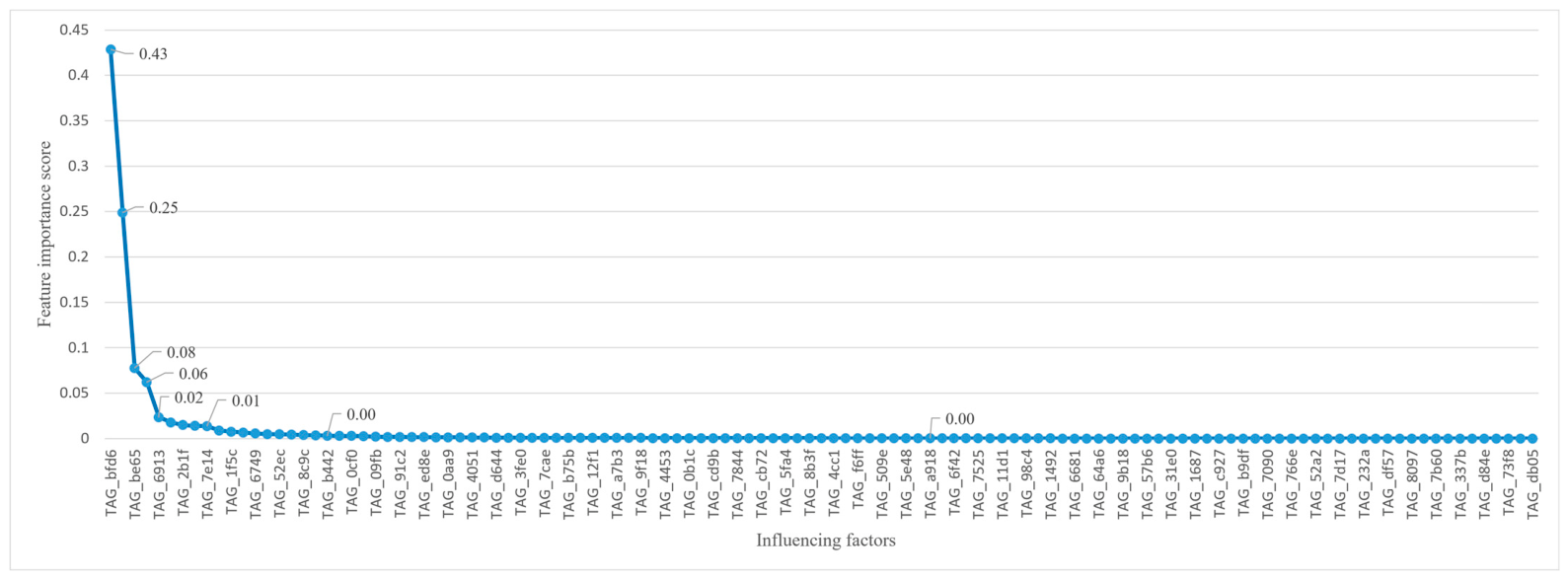
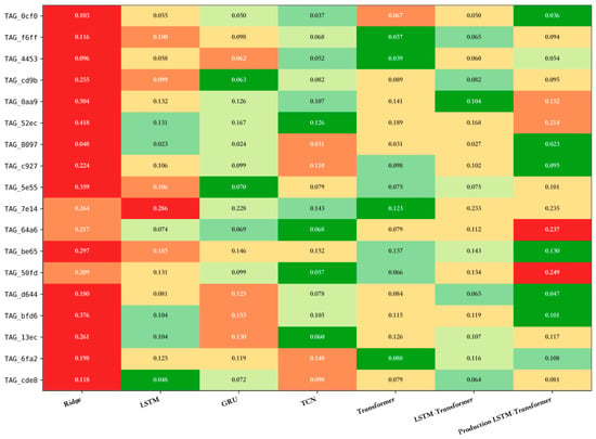
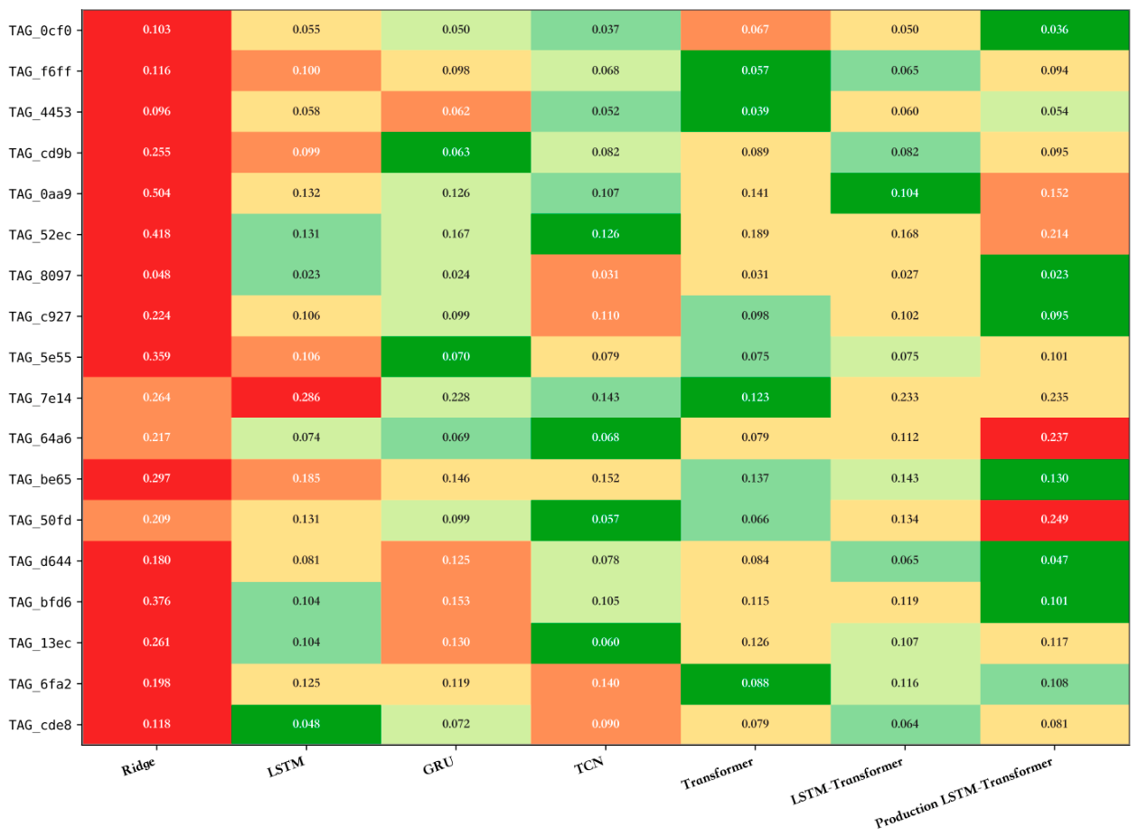
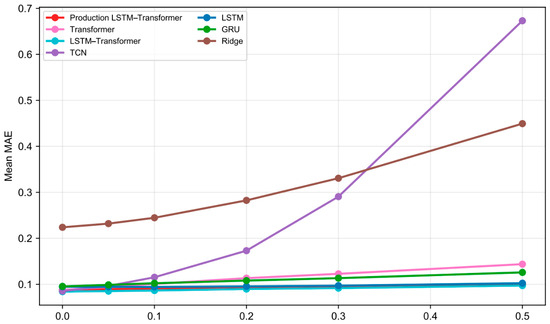
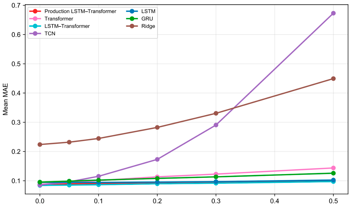
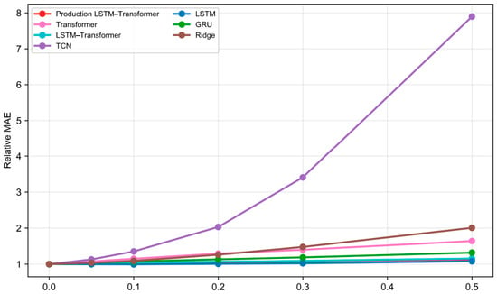
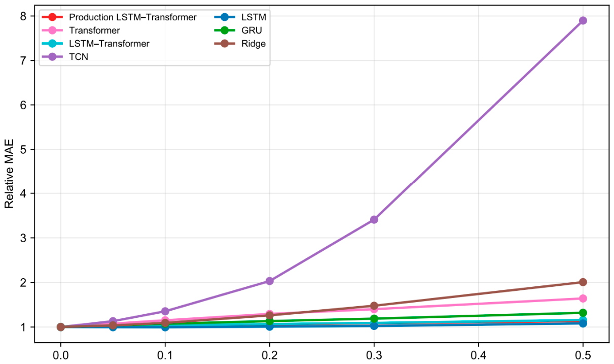
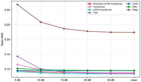
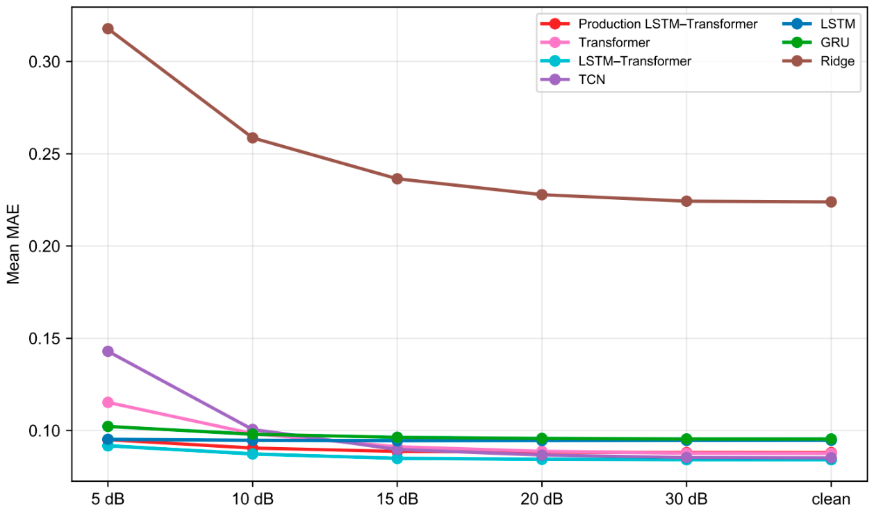
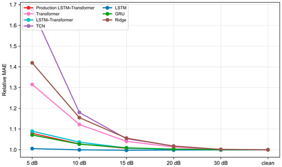
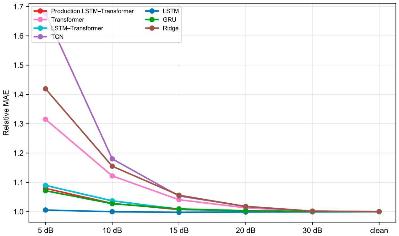

Disclaimer/Publisher’s Note: The statements, opinions and data contained in all publications are solely those of the individual author(s) and contributor(s) and not of MDPI and/or the editor(s). MDPI and/or the editor(s) disclaim responsibility for any injury to people or property resulting from any ideas, methods, instructions or products referred to in the content. |
© 2026 by the authors. Published by MDPI on behalf of the International Institute of Knowledge Innovation and Invention. Licensee MDPI, Basel, Switzerland. This article is an open access article distributed under the terms and conditions of the Creative Commons Attribution (CC BY) license.