


Abstract
Alzheimer’s disease (AD) is the most prevalent neurodegenerative disorder worldwide, affecting approximately 56.9 million people in 2021 and projected to reach 152 million by 2050. Its defining pathological features, amyloid-beta plaques and neurofibrillary tangles, accumulate for up to two decades before cognitive symptoms emerge, placing the preclinical and mild cognitive impairment (MCI) stages at the centre of the early detection problem. Despite this, current diagnostic practice in routine clinical settings remains unreliable, with post-mortem studies placing the specificity of clinical AD diagnosis between 44.3 and 70.8% even in specialist memory clinics. Machine learning (ML) and deep learning (DL) applied to neuroimaging and electrophysiological data have emerged as candidate tools for closing this diagnostic gap, yet whether the accuracy figures reported in published studies translate into clinically useful performance on independent data remains unresolved. This study presents a structured comparative review of machine learning and deep learning methods reported across four publicly available Alzheimer’s disease datasets, namely the Alzheimer’s Disease Neuroimaging Initiative (ADNI), the Open Access Series of Imaging Studies (OASIS), the OpenNeuro ds004504 electroencephalography (EEG) dataset, and the Kaggle Alzheimer’s magnetic resonance imaging (MRI) dataset. Thirteen model families are examined through the published literature rather than through new experiments, and for each model and dataset combination, the best accuracy reported in the source study is recorded alongside the model’s mathematical formulation. All performance figures reported in this abstract and throughout the paper are taken from the published studies reviewed, not from new experiments conducted by the authors. Across the reviewed studies, deep learning architectures pre-trained on ImageNet and fine-tuned on neuroimaging data are reported to produce the highest accuracy on MRI classification tasks. Residual Network (ResNet)-101 is reported at 98.21 percent on ADNI and 97.45 percent on OASIS, while the IncepRes fusion architecture reaches 98.35% on OASIS by combining multi-scale feature extraction from InceptionV3 with residual connectivity from ResNet152V2. Traditional machine learning classifiers remain competitive on tabular clinical and biomarker data, with Extreme Gradient Boosting (XGBoost) reaching 91% on ADNI multiclass features. Logistic Regression achieves 82 to 85% on binary ADNI classification and is the only classifier in this review that provides explicit per-feature prediction contributions without post hoc tooling. Gaussian Naïve Bayes achieves 80 to 83% on the same task. On the OpenNeuro EEG dataset, K-nearest neighbours (KNN) with singular value decomposition (SVD) entropy features achieves 91% binary accuracy, with feature engineering quality determining performance more reliably than classifier architecture. Eight principal findings emerge from the cross-dataset analysis. Binary classification consistently outperforms multiclass by 10 to 30% across all datasets, reflecting the genuine biological ambiguity of the mild cognitive impairment category. Dataset size and augmentation predict reported accuracy more reliably than model architecture. Ensemble methods outperform individual classifiers by 5 to 8% in nearly every imaging study. Deeper architectures can overfit small clinical cohorts. EEG models trail MRI models by approximately 10 to 15% on comparable binary tasks. Cross-dataset generalisation has not been systematically evaluated in most studies, and the few that have tested it report accuracy drops of 5 to 10% or more when models encounter data from different scanners or cohorts. Eight recurring limitations constrain the clinical utility of these findings. Small sample sizes and limited demographic diversity, severe class imbalance inflating raw accuracy metrics, poor cross-dataset generalisation driven by scanner heterogeneity, limited deep learning interpretability, the dominance of binary over multiclass tasks, the absence of longitudinal modelling despite available datasets, inadequate standardisation of preprocessing and evaluation protocols, and the signal-to-noise ratio constraints specific to EEG recordings of elderly patients collectively define the gap between benchmark performance and clinical readiness. Future work must prioritise multi-centre training cohorts, multimodal fusion architectures, longitudinal progression modelling, and standardised interpretability evaluation as non-optional requirements for any system intended for clinical deployment.
1. Introduction
1.1. Background and Significance
Alzheimer’s disease (AD) is the most common neurodegenerative disorder, characterised by its progressive nature and resulting in significant cognitive decline [1,2,3]. As a reforming disorder, AD is pathologically defined by the presence of β-amyloid (Aβ) plaques and neurofibrillary tangles (NFTs) [1,4]. It is an irreversible condition characterised by the gradual destruction of neuronal networks responsible for memory, language, executive function, and behavioural regulation, ultimately leaving affected individuals entirely dependent on full-time care [5]. Given that its prevalence is expected to be more than double the amount by 2050 due to the ageing global population, AD is among the most urgent health challenges of ageing societies [3]. A crucial element in managing this disease is early detection, as interventions and disease-modifying therapies are believed to be most effective if administered early in the disease course, prior to the onset of irreversible brain damage [1,2,6]. However, symptoms often progress gradually, leading to delayed diagnoses, with a substantial proportion of patients diagnosed only at the moderate stage [2].
The global scale of the condition is staggering and growing. As of 2021, approximately 56.9 million people worldwide were living with Alzheimer’s disease and other dementias, representing a 160 percent increase from the 21.9 million cases recorded in 1990 [7]. The World Health Organisation estimates that roughly 10 million new cases emerge each year, translating to one new diagnosis every three seconds [8]. Demographic projections intensify the urgency considerably. As the proportion of the global population aged 60 and over is expected to nearly double from 12% in 2015 to 22% by 2050, the number of people with Alzheimer’s disease is forecast to reach 152 million by the same year if no effective intervention is established [9].
Beyond its neurological devastation, the condition stands as the costliest of the twenty-first century. In the United States alone, total healthcare expenditures related to Alzheimer’s disease and related dementias reached an estimated 321 billion dollars in 2022, a figure projected to surpass one trillion dollars annually by 2050 [5]. As reported in the systematic review by Tay et al. [10], the global cost of dementia care is expected to reach two trillion dollars by 2030. Caregiving is the single largest cost component. An estimated 360 billion dollars was spent on health and long-term care in the United States in 2024 alone, with unpaid informal caregiving adding an additional 271 billion dollars in economic value [11]. The burden falls disproportionately on families and healthcare systems across low- and middle-income countries, where the infrastructure for diagnosis and management is most severely constrained [7].
Early detection in Alzheimer’s disease is constrained by the disease’s long preclinical phase, during which pathology accumulates without measurable cognitive change. Amyloid-beta plaques and hyperphosphorylated tau tangles start building up in the brain about two decades before a patient shows any clinical symptoms [12]. Amyloid PET imaging studies have shown that subtle markers of neurodegeneration, such as reduced glucose metabolism in temporal and parietal cortical regions, can be picked up more than 20 years before a patient crosses the amyloid positivity threshold that clinicians use as the diagnostic boundary for preclinical AD [13]. By the time memory loss and cognitive decline are clinically obvious, much of the underlying neuronal damage has already happened. Because the trajectory is progressive and irreversible, intervention strategies work better the earlier they start [14].
Between the extended asymptomatic preclinical phase and the overt dementia stage lies a transitional period known as mild cognitive impairment (MCI). Characterised by measurable deficits in memory and other cognitive domains that do not yet interfere significantly with daily living, MCI is widely understood as the most clinically actionable window for intervention [15]. Studies consistently report that between 10 and 15% of individuals with MCI progress to Alzheimer’s dementia annually, with cumulative conversion rates of 30 to 40% over five years [16]. Among those with amnestic MCI confirmed by amyloid biomarkers, progression can occur in more than 50% of cases within three years [13]. Identifying which MCI patients will convert, and how quickly, is therefore one of the central unsolved problems in Alzheimer’s disease research and the core motivation for applying machine learning to progression modelling [9].
1.2. The Diagnostic Challenge
The clinical diagnosis of Alzheimer’s disease in routine practice remains predominantly based on neuropsychological assessment tools such as the Mini-Mental State Examination (MMSE), the Montreal Cognitive Assessment (MoCA), and the Clinical Dementia Rating scale (CDR), supplemented where available by structural magnetic resonance imaging (MRI) showing hippocampal atrophy [17]. These approaches, while practical and accessible, carry substantial diagnostic uncertainty. As reported in the diagnostic review by Vyhnalek et al. [17], post-mortem neuropathological studies place the specificity of clinical AD diagnosis, even in specialist memory clinics, between only 44.3 and 70.8 percent. Memory impairment and hippocampal atrophy, the two most relied-upon clinical markers, are present in several other neurodegenerative conditions, including frontotemporal dementia, Lewy body dementia, and vascular dementia, limiting their diagnostic discriminative value [12].
Standard cognitive screens were built to catch moderate or severe dementia, not the subtle changes seen in early MCI, so they perform poorly at the stage where it matters most. Mekulu et al. [18] argue that by the time patients score positive on tests like the MMSE, they are often past the window where disease-modifying therapies do their best work. Patients in community settings often wait six to twelve months for a specialist neuropsychological assessment or imaging appointment, which is a long time given that the neuronal loss during this period cannot be reversed [18].
Biomarker-based diagnosis, incorporating cerebrospinal fluid (CSF) measurements of amyloid-beta 42, phosphorylated tau, and total tau, or amyloid and tau PET imaging, offers superior sensitivity and specificity. The 2024 Alzheimer’s Association revised diagnostic criteria formalised a biologically defined staging framework grounded in these markers [19]. However, CSF collection requires lumbar puncture, which carries procedural risk and patient reluctance. PET imaging is expensive, requires radiopharmaceutical infrastructure, and is unavailable in most low- and middle-income health systems [20]. Even in high-income settings, access to these investigations is unevenly distributed. The gap between what biomarker-based criteria can theoretically achieve and what routine clinical practice delivers at scale remains wide, and it is precisely this gap that computational approaches to diagnosis are positioned to address [21].
1.3. Machine and Deep Learning Approaches to Alzheimer’s Disease Detection
The past decade has seen a substantial surge in the application of machine learning (ML) and deep learning (DL) techniques to Alzheimer’s disease detection and classification. A scoping review covering 2018 to 2024 found that the majority of recent studies applied convolutional neural networks (CNNs) or transfer learning architectures and reported internal test accuracies above 90% across a variety of modalities [22]. The breadth of data modalities exploited has also expanded considerably, encompassing structural MRI, functional MRI, diffusion tensor imaging, FDG-PET, amyloid PET, electroencephalography (EEG), clinical cognitive scores, CSF biomarkers, and genetic markers such as APOE genotype [23].
Traditional ML classifiers, including Support Vector Machines (SVMs), Random Forests (RF), Extreme Gradient Boosting (XGBoost), K-Nearest Neighbours (KNN), Logistic Regression, and Gaussian Naïve Bayes, have been successfully applied to tabular clinical and biomarker data extracted from large repositories such as the Alzheimer’s Disease Neuroimaging Initiative (ADNI) [21,24,25,26,27]. Results demonstrated that XGBoost achieved 91% accuracy on ADNI multiclass clinical data, outperforming SVM and Random Forest by exploiting native handling of missing values and sequential error correction [24]. Ensemble voting approaches combining multiple classifiers have further extended performance, with results reporting 90.6% balanced accuracy on binary healthy control versus AD classification across both ADNI and OASIS cohorts [21].
Deep learning architectures operating directly on neuroimaging data have produced the highest reported accuracy figures in the study. Transfer learning approaches using architectures pre-trained on ImageNet, particularly ResNet variants and DenseNet, have proven especially effective when adapted to MRI classification tasks. Results reported 98.21% multiclass accuracy on ADNI and 97.45% on OASIS using ResNet-101 with ImageNet initialisation, outperforming shallower and deeper ResNet variants as well as DenseNet-201 and EfficientNet-B0 on the same datasets [28]. Ensemble architectures fusing multiple transfer learning backbones have pushed performance further still. IncepRes was used to combine the multi-scale parallel feature extraction of InceptionV3 with the residual connectivity of ResNet152V2, achieving 98.35% on OASIS and 96.96% on ADNI [29].
Electroencephalography offers a distinct and clinically valuable modality for Alzheimer’s disease research. EEG is non-invasive, lower in cost than MRI or PET, and can be recorded continuously, making it a natural candidate for longitudinal monitoring applications. The neurophysiological basis for EEG-based classification lies in well-documented changes in spectral power distribution in AD, particularly the reduction in alpha band power (8 to 13 Hz) and the elevation of delta and theta power relative to healthy controls [30]. The OpenNeuro ds004504 dataset, which contains resting-state EEG recordings from 36 AD patients, 23 frontotemporal dementia (FTD) patients, and 29 healthy controls, has become the principal open-access resource for EEG-based AD classification research [31]. Studies applying graph signal processing, microstate analysis, and functional connectivity features to this dataset have reported binary dementia versus healthy control accuracies ranging from 79 to 91 percent [32,33].
Although the reported accuracy figures appear high, several methodological factors limit how reliably they reflect performance on independent clinical data. Most studies train and test their models on the same dataset, using cross-validation or holdout splits drawn from the same cohort. This means the test accuracy reflects how well the model handles data that looks like the training set, not data from a new hospital or scanner. A survey of ML models for AD diagnosis found that within-dataset accuracies of 97 to 99% collapsed to 50 to 67% when tested on different cohorts or acquisition protocols [34]. The generalisation gap this exposes is arguably the biggest barrier to clinical use of these models. A model with 98% within-dataset accuracy that falls to 70% on a new hospital’s scanner is not useful in practice [22].
Further challenges stem from severe class imbalance in available datasets, the absence of standardised preprocessing pipelines across studies, the predominance of binary (AD versus healthy control) rather than clinically meaningful multiclass tasks, and the limited interpretability of complex deep learning models. Black-box architectures present a substantial barrier to clinical adoption, where clinicians require explanations for model predictions in order to integrate automated outputs into diagnostic decision making [35]. Regulatory requirements in most jurisdictions additionally mandate explainability for AI-based medical devices. The field is therefore moving toward hybrid approaches that combine high-accuracy DL architectures with post hoc interpretability methods such as Grad-CAM saliency mapping, SHAP values, and attention weight visualisation [23].
1.4. Problem Statement
The problem this study addresses is the gap between how well ML and DL models perform in research papers and what they would need to do in a clinical setting. Three specific problems underlie this.
Problem 1: The early detection gap: Alzheimer’s disease pathology is present and measurable for up to two decades before a patient receives a clinical diagnosis, yet diagnostic practice in most healthcare settings still relies on symptom-driven referral [12,13]. By the time a diagnosis is confirmed, the window for the most effective pharmacological and lifestyle interventions has often closed. The MCI stage, where 10 to 15 percent of individuals convert to dementia annually, shows the critical juncture where automated detection systems could materially alter the clinical trajectory for a patient, yet it is also the stage where classification is most difficult because MCI occupies a continuous biological spectrum between normal ageing and established dementia. The core problem is that current diagnostic tools are better calibrated for confirming disease than for detecting its earliest manifestations, as it is difficult to detect AD in its earlier stages [36].
Problem 2: The dataset specificity problem: Machine learning models developed for Alzheimer’s disease detection are overwhelmingly trained and evaluated on a small number of widely used research repositories: ADNI, OASIS, the Kaggle MRI dataset, and the OpenNeuro EEG dataset ds004504. These datasets share important characteristics that limit their representativeness, including predominantly North American and European participant pools, acquisition protocols specific to high-field research scanners, strict clinical trial eligibility criteria that exclude common comorbidities, and relatively small sample sizes that produce high variance in reported metrics. A model trained exclusively on ADNI data carries implicit scanner-specific and demographic biases that prevent reliable deployment in a diverse clinical setting [37]. The problem is therefore not only one of achieving high accuracy but of demonstrating that accuracy is stable across the distribution shifts that characterise real-world clinical applications.
Problem 3: The modality integration problem: Different data modalities provide complementary diagnostic information. Multimodal integration can be organised into three broad strategies. Early fusion combines raw or low-level features from each modality into a single input vector before classification. Late fusion trains a separate model per modality and combines their outputs, for example, by averaging predicted probabilities or by majority voting. Hybrid fusion combines intermediate representations at one or more stages of the model. A deployable system must also handle missing modalities, since not every patient has MRI, EEG, cognitive, and biomarker data available at every visit, which favours architectures able to produce a prediction from whichever modalities are present. Structural MRI reveals macroscopic atrophy patterns in the hippocampus and temporal cortex. EEG captures electrophysiological changes in synchrony and spectral power that reflect network-level disruption. Cognitive assessments quantify the behavioural manifestation of neurodegeneration. CSF and plasma biomarkers provide molecular-level confirmation. Each modality has distinct cost, invasiveness, and availability profiles. MRI offers high specificity but requires expensive imaging infrastructure; EEG is cheaper and non-invasive but noisier and more susceptible to artefact; cognitive scores are universally accessible but sensitive to education, language, and cultural factors. The existing literature overwhelmingly evaluates these modalities in isolation rather than in combination, leaving the question of optimal multimodal integration for real-world monitoring systems quite unresolved [23,38].
These three problems converge on a single gap that this study addresses, which is the need for a systematic, evidence-based evaluation of how well established and contemporary machine learning and deep learning models perform across multiple publicly available Alzheimer’s disease datasets and modalities, with attention to the factors that explain performance variation and the conditions that would need to be satisfied for such models to operate reliably in a clinical setting. Rather than proposing a novel architecture, this study conducts a structured review and comparative analysis of the methods, datasets, and results documented in the current literature, with the goal of establishing a clear and honest account of what has been achieved, where the boundaries of current capability lie, and what the most productive directions for future work appear to be [22,37].
1.5. Research Aims and Objectives
The aim of this study is to provide a rigorous, evidence-based comparative analysis of machine learning and deep learning methods applied to Alzheimer’s disease detection across neuroimaging and electrophysiological datasets. The objectives are as follows:
- ◦
- To identify and characterise the principal publicly available datasets used for ML-based AD classification research, documenting their design, demographic composition, class distribution, available modalities, and known limitations relevant to model development and evaluation.
- ◦
- To present a comprehensive technical description of the machine-learning pipeline and the machine learning and deep learning models most frequently applied in the reviewed literature, including a formalisation of preprocessing, feature extraction, feature selection, dataset partitioning, and model training stages, full mathematical formulations for six traditional ML classifiers (SVM, RF, XGBoost, KNN, Logistic Regression, and Gaussian Naïve Bayes) and seven DL architectures (CNN, ResNet, VGG, DenseNet, EfficientNet, Inception, and ViT), and to contextualise each model’s theoretical properties in relation to the specific characteristics of the dataset under evaluation.
- ◦
- To compile and compare the performance results reported across the reviewed studies, organising comparisons within each dataset to enable fair assessment of relative model performance under equivalent conditions.
- ◦
- To analyse the sources of performance variation across models and datasets, including the roles of dataset size and augmentation, class imbalance, task framing (binary versus multiclass), feature modality, and model architecture depth.
- ◦
- To critically evaluate the limitations documented in the review literature and identify the key gaps that must be addressed before ML-based Alzheimer’s disease detection systems can transition from research settings to meaningful clinical deployment.
1.6. Significance and Contribution
This study contributes to the literature in three specific ways. Firstly, it brings together results from studies using four distinct datasets and seven distinct model families into a single structured comparison that is currently absent from the literature. Most existing reviews either focus on a single modality, a single dataset, or a single model class, making cross-dataset and cross-modality interpretation difficult. Furthermore, the methodological sections provide an unusually detailed mathematical summary of the models most applied to Alzheimer’s disease classification, presented so that the technical content remains accessible to researchers from clinical neuroscience backgrounds who may not have primary training in machine learning. Alongside this, the comparative analysis and problem statement directly address the generalisation deficit that the broader literature has identified as the primary barrier to clinical translation, providing a concrete evidence base from which future work can proceed [23,37,39].
The findings of this study are relevant to clinicians, health informaticians, and data scientists working on automated dementia screening tools; to policymakers seeking an honest assessment of AI readiness for clinical dementia services; and to researchers designing the next generation of Alzheimer’s disease detection studies who need to understand the strengths and failure modes of existing approaches before proposing improvements. Validation in this field can be placed on four levels of increasing clinical relevance. Within-dataset cross-validation resamples a single cohort and is the most common and weakest. External cohort validation tests a trained model on a separate, independently collected dataset. Cross-scanner validation further tests robustness to changes in acquisition hardware and protocol. Prospective clinical validation evaluates the model on patients seen after it was fixed, under routine conditions. This review uses these four levels as an organising principle: most reported accuracies arise from within-dataset cross-validation, while the levels that determine clinical usefulness are rarely reached.
2. Materials and Methods
The methodological framework adopted in this review is presented in this chapter. It covers the selection and description of the datasets used, the ML and DL models evaluated, the mathematical formulations underpinning each model, the experimental setup, and the performance metrics used to assess model outcomes. The chapter concludes with a comparative analysis of results across all models and datasets.
2.1. Search Strategy and Study Selection
This review was conducted and reported in accordance with the Preferred Re-porting Items for Systematic Reviews and Meta-Analyses (PRISMA) 2020 statement [40]; the completed PRISMA 2020 checklist is provided in the Supplementary Materials (Table S1). The studies reviewed were identified through a structured search of Google Scholar, IEEE Xplore, PubMed, and ScienceDirect, covering the period January 2011 to May 2025 (The date window applies to the search for primary classification studies; foundational methodological, architectural, and dataset-descriptor references are cited outside this window where appropriate.). Search terms combined the disease domain with the methodological domain, using strings such as (“Alzheimer’s disease” OR “mild cognitive impairment”) AND (“machine learning” OR “deep learning” OR “convolutional neural network” OR “transfer learning”) AND (“ADNI” OR “OASIS” OR “EEG” OR “MRI”). A study was included if it reported quantitative classification performance for Alzheimer’s disease or mild cognitive impairment on at least one of the four datasets examined in this review, was written in English, and described its model and evaluation protocol in enough detail to be interpreted. A study was excluded if it reported no usable performance metric, did not use one of the four datasets, was not peer reviewed, or was a redundant report of a cohort already represented.
The search returned 286 records. After 39 duplicates were removed, 247 records were screened by title and abstract, of which 142 were excluded. Of the 105 reports sought for retrieval, five could not be obtained, leaving 100 reports assessed in full. A further 85 were excluded as not relevant, namely 33 that did not use one of the four datasets, 24 with no usable performance metric, 17 that were not peer reviewed, and 11 that were redundant reports of an already included cohort. Fifteen primary studies met all criteria and form the evidence base synthesised in Section 3. The selection process is summarised in Figure 1. Consistent with the structure of a literature review, this work synthesises the results reported in these primary studies rather than generating new experimental results [22].
Figure 1.
PRISMA 2020 flow diagram of the study identification, screening, and inclusion process.
2.2. Datasets
The four datasets differ in their unit of analysis, and this distinction matters for interpreting reported accuracy. ADNI, OASIS, and the OpenNeuro EEG dataset are subject-level datasets, in which each subject contributes one or more scans or recordings, and splits can be made so that no subject appears in both training and test sets. The Kaggle MRI dataset is distributed as individual image slices without subject identifiers, so slices originating from the same subject or the same preprocessing pipeline can appear in both splits. Where subject-level separation cannot be guaranteed, reported accuracy may be inflated by within-subject similarity rather than reflecting generalisation to new patients.
2.2.1. Alzheimer’s Disease Neuroimaging Initiative (ADNI)
ADNI is the gold standard neuroimaging repository for AD research and is the most cited dataset in the ML-based AD literature. Its longitudinal design enables both cross-sectional classification and progression modelling. The five diagnostic categories are cognitively normal (CN), subjects with significant memory concern (SMC), early MCI (EMCI), late MCI (LMCI), and AD. Classification difficulty escalates noticeably when MCI subgroups are included because the structural brain changes in EMCI overlap with both CN and LMCI. MMSE and CDR-SOB scores are provided at every visit alongside imaging data, allowing multimodal feature construction. Missing data is a known challenge in ADNI, as not all subjects undergo all modalities at every visit. Table 1 shows the relevant data regarding the ADNI dataset [21,24].
Table 1.
ADNI dataset information [40,41].
2.2.2. Open Access Series of Imaging Studies (OASIS)
OASIS is widely used as a benchmark because it requires no institutional application and provides pre-processed FreeSurfer volumetric measurements alongside raw MRI scans. The primary class label is the Clinical Dementia Rating (CDR) score, which maps onto the four classes listed above. The severe class imbalance in OASIS-1, where non-demented subjects account for approximately 76% of all observations, is a critical methodological issue that must be addressed through oversampling techniques such as SMOTE or through class-weighted loss functions. Studies that do not account for this imbalance report artificially elevated accuracy figures. OASIS-3 extends the dataset longitudinally with multimodal imaging, making it more comparable to ADNI in scope. Research using merged ADNI and OASIS datasets has demonstrated improved generalisation compared to either dataset in isolation. Table 2 shows the relevant data regarding the OASIS dataset [29,42,43].
Table 2.
OASIS dataset information [44,45].
2.2.3. OpenNeuro ds004504 (EEG Dataset)
This dataset is the principal publicly available EEG resource for AD and FTD classification research and is the same dataset used in earlier stages of this project. Its clinical recording setting and the inclusion of both AD and FTD groups make it particularly valuable for testing whether models can differentiate between distinct neurodegenerative conditions rather than simply separating pathological from healthy brain activity. Key signal features extracted from EEG recordings include spectral power across five canonical frequency bands (delta: 0.5 to 4 Hz; theta: 4 to 8 Hz; alpha: 8 to 13 Hz; beta: 13 to 30 Hz; and gamma: 30 to 45 Hz), functional connectivity metrics computed between electrode pairs, entropy-based complexity measures, and microstate dynamics. Alpha power reduction and delta/theta power elevation are the most established EEG biomarkers of AD. The small sample size of 88 subjects is the primary limitation of this dataset and produces high variance in reported accuracy across studies. Table 3 shows the relevant data regarding the OpenNeuro dataset [30,46].
Table 3.
OpenNeuro dataset information [31].
2.2.4. Kaggle Alzheimer’s MRI Dataset
The Kaggle dataset is the most widely used benchmark for transfer learning-based AD classification due to its accessibility and pre-processed format, which requires no raw MRI processing pipeline. The four classes map onto CDR severity levels consistent with OASIS labelling. Despite producing the highest reported accuracy figures in the literature (97 to 99.7%), results on this dataset must be interpreted with caution. The test set is sampled from the same distribution as the training set, which does not reflect the scanner diversity, demographic variation, or protocol differences encountered in real clinical deployment. The extreme imbalance in the ModerateDemented class (64 images out of 6400) means models evaluated without class imbalance correction are effectively penalised on the minority class. The Kaggle dataset is both heavily imbalanced across its four classes and limited in distribution, having been derived from a small pool of source images expanded by augmentation. The very high accuracies reported on this dataset, which reach 99.68 percent for a convolutional network trained on approximately 80,000 augmented slices, reflect performance on augmented copies of a narrow image distribution. They are not comparable to subject-level diagnosis on independent cohorts and should not be interpreted as evidence of clinical accuracy. SMOTE application is therefore standard practice before training. Table 4 shows the relevant data regarding the Kaggle MRI dataset [28,34,47,48].
Table 4.
Kaggle dataset information [28,47].
2.3. Machine Learning Pipeline
The pipeline presented in Figure 2 is a synthesis of the common structure observed across the reviewed studies, offered as a reference framework rather than a protocol that every study followed identically. As documented in the reviewed literature [21,24,28,29,30,31,42,46,47,49,50,51,52,53], most studies can be described in terms of six successive stages, namely data acquisition and preprocessing, feature extraction, feature selection or dimensionality reduction, dataset partitioning, model training and hyperparameter tuning, and evaluation. Individual studies differ in which stages they emphasise and in the specific operations performed at each stage, particularly between imaging and electrophysiological modalities. Table A1 contains a summary of all mathematical notations and variable definitions used in this review.
Figure 2.
Pipeline block diagram.
2.3.1. Data Acquisition and Preprocessing
Preprocessing converts raw data into a normalised representation suitable for machine learning. For MRI data, the standard sequence is N4 bias-field correction, skull stripping with FSL BET or U-Net-based approaches, spatial registration to a standard template such as MNI152 with ANTs or SPM, intensity normalisation, and optional voxel-based morphometry to produce voxel-wise grey-matter density maps [28,29,42,46,47,54,55,56]. For EEG data, preprocessing comprises band-pass filtering (typically 0.5–45 Hz), artefact removal via Artefact Subspace Reconstruction (ASR) or independent component analysis (ICA), re-referencing to the common-average reference, and epoching into fixed-length segments [30,31,32,33,46,57,58]. For tabular biomarker data, preprocessing comprises missing-value imputation (mean, median, or K-nearest-neighbour imputation), z-score normalisation, and one-hot encoding of categorical variables [21,24,51,52].
Two normalisation schemes appear in the reviewed literature. Z-score normalisation given in Equation (1) scales each feature to zero mean and unit variance, while min–max normalisation given in Equation (2) maps each feature to the interval [0, 1] [52,53].
where x is the raw feature value; μ and σ are the mean and standard deviation of the feature across the training set; min and max are the minimum and maximum values of the feature across the training set. Z-score normalisation is preferred for classifiers that assume Gaussian feature distributions (Logistic Regression, Gaussian Naïve Bayes, SVM with RBF kernel). Min–max normalisation is preferred for distance-based classifiers such as KNN [52,53].
2.3.2. Feature Extraction
Feature extraction converts the preprocessed data into a fixed-length feature vector that summarises the diagnostically relevant information. The reviewed studies use four broad categories of features.
- Structural MRI features: voxel-wise grey-matter density, regional volumes (hippocampus, entorhinal cortex, ventricles) extracted with FreeSurfer, and cortical thickness measurements [21,24,28,42,47].
- EEG features: power spectral density in the delta (0.5–4 Hz), theta (4–8 Hz), alpha (8–13 Hz), beta (13–30 Hz), and gamma (30–45 Hz) bands; Graph Discrete Fourier Transform connectivity features; microstate temporal dynamics; and Singular Value Decomposition entropy [30,32].
- Clinical and demographic features: MMSE, CDR-SB, ADAS-Cog scores; APOE genotype; CSF biomarkers (Aβ42, p-tau, t-tau) extracted directly from the ADNI tabular files [21,24,42].
- Implicit deep-learning features: the activations of the final pooling, projection, or class-token layer of CNN, ResNet, DenseNet, EfficientNet, Inception, and ViT architectures used as feature vectors for downstream classifiers in transfer-learning pipelines [28,29,47,59].
2.3.3. Feature Selection and Dimensionality Reduction
Feature selection retains the subset of extracted features most informative for classification, reducing both overfitting risk and computational cost [60]. Three approaches dominate the reviewed literature.
Filter methods rank each feature by its individual association with the class label and retain the top-K. Spearman’s rank correlation given in Equation (3) is used by Li et al. [24] on ADNI tabular features to retain the 30 features most correlated with diagnosis. Mutual Information given in Equation (4) is used as an alternative to capture non-linear dependencies between features and class labels [24,60].
where di is the rank difference between the feature value and the class label for sample i; n is the number of samples; p(x, y) is the joint probability of feature value x and class label y; p(x) and p(y) are the marginal probabilities. ρ close to ±1 indicates a strong monotonic association, while I(X; Y) is zero for independent features and grows with their statistical dependence [60].
Wrapper methods evaluate feature subsets by training the classifier and measuring cross-validation accuracy. Recursive Feature Elimination (RFE) with an SVM classifier is the most widely used wrapper in AD biomarker studies [21,27].
Embedded methods perform feature selection during model training. The Random Forest variable-importance score and the XGBoost gain-based importance are embedded selectors used to rank features after model fitting [24,26].
Principal Component Analysis (PCA) performs linear dimensionality reduction by projecting features onto the K orthogonal directions of maximum variance. The k-th principal component is given in Equation (5) [21,61].
where vk is the k-th eigenvector of the feature covariance matrix Σ = (1/n) Σi (xi − )(xi − )T, ordered by descending eigenvalue λk; is the mean feature vector across the training set; zk is the projection of sample x onto the k-th principal axis. The first K components are retained such that the cumulative explained variance ratio Σk λk/Σj λj exceeds a chosen threshold, commonly 0.90 or 0.95 [61].
2.3.4. Dataset Partitioning
The reviewed studies use three dataset-partitioning protocols. Hold-out splits divide the data into fixed training (typically 70–80%), validation (10–15%), and test (10–15%) sets used once; this is the protocol of the Kaggle ALZENET study and of the ResNet-101 ADNI study. K-fold cross-validation divides the data into k equally sized folds, trains the model k times (each time on − 1 folds and tested on the remaining fold), and reports the mean score across folds. Five-fold and ten-fold are the most common settings. The k-fold cross-validation error is given in Equation (6) [21,24,28,29,47,51].
where is the number of folds (typically 5 or 10); L(·) is the loss or error rate on the i-th fold; f−i is the model trained on all folds except the i-th; Di is the i-th held-out fold used for evaluation. Leave-One-Subject-Out cross-validation (LOSO) is used in EEG studies with limited subject counts, e.g., ds004504 with 88 subjects. Each subject is held out once, the model is trained on all other subjects, and tested on the held-out subject. LOSO eliminates within-subject data leakage but produces high-variance estimates when the test fold contains only one subject [31,46,51,53].
Two leakage-control conditions are required for any of these protocols to produce valid estimates on image data. First, splitting must be performed at the subject level, so that all slices or recordings from a given subject fall entirely within either the training or the test set and never both. Second, any class-balancing or augmentation operation, such as SMOTE oversampling or image augmentation, must be applied only within the training fold after the split, never before it, so that synthetic or augmented samples derived from test subjects cannot leak into training. These conditions are particularly important for the Kaggle MRI dataset, which is highly imbalanced and is distributed as individual slices without subject identifiers, making subject-level separation difficult to guarantee. Where the reviewed studies do not state how splitting and augmentation were ordered, their reported accuracy should be treated as an upper bound [34,47].
2.3.5. Model Training and Hyperparameter Tuning
Traditional ML models are trained by optimising their respective loss functions defined in Section 2.5. Hyperparameters that cannot be learnt from data, such as SVM regularisation parameter C and kernel bandwidth γ, Random Forest tree count T and feature subset size m, XGBoost learning rate η and maximum tree depth, KNN neighbourhood size K, Logistic Regression regularisation strength λ, and Gaussian Naïve Bayes variance smoothing constant ε, are tuned by grid search or random search over a held-out validation subset. Bayesian optimisation is used for the ALZENET ensemble. Deep-learning models are trained using the shared components defined in Section 2.4 [47,51,53].
2.3.6. Evaluation
Final model performance is reported using the metrics defined in Section 2.7. The reviewed studies report accuracy as the primary metric. Statistical-significance testing of differences between models is rarely reported, which is itself a methodological limitation discussed in Section 4.2.8 [62,63,64].
2.4. Shared Training Components
The shared training components used by the deep learning models, namely categorical cross-entropy loss given in Equation (A1), softmax output given in Equation (A3), ReLU activation given in Equation (A4), batch normalisation given in Equations (A5)–(A8), max pooling given in Equation (A9), dropout given in Equation (A10) and Adam optimisation given in Equations (A11)–(A15), are standard across modern deep learning, and their full formulations are provided in Appendix A. The main text retains the model-specific formulations in Section 2.5 and Section 2.6, together with a short statement of each model’s assumptions, suitability for Alzheimer’s disease data, and limitations [65,66,67,68,69,70,71].
2.5. Machine Learning Models
Six ML classifier families are reviewed in this paper, such as Support Vector Machine, Random Forest, XGBoost, K-Nearest Neighbours, Logistic Regression, and Gaussian Naïve Bayes. SVM, RF, XGBoost, and KNN represent margin-based, ensemble-tree, and instance-based approaches. Logistic Regression and Gaussian Naïve Bayes are added as interpretable baselines that appear consistently as comparators across the AD-detection literature.
2.5.1. Support Vector Machine (SVM)
The Support Vector Machine constructs the maximum-margin hyperplane separating two classes in a high-dimensional feature space. For a training set of n labelled samples (, ) where is a d-dimensional feature vector and in {−1, +1} is the binary class label, the primal hard-margin optimisation problem is given in Equation (7), subject to Equation (8).
where w ∈ (d-dimensional real space) is the weight vector defining the orientation of the hyperplane; ||w||2 is the squared L2 norm of w (equal to ); minimising this maximises the geometric margin, which equals 2/||w||; b is the scalar bias (intercept) determining the hyperplane offset from the origin; is the dot product , producing the signed distance of from the hyperplane; >= 1 is the constraint ensuring every sample is on the correct side of the margin with a clearance of at least 1/||w||. For real-world non-separable data, slack variables >= 0 are introduced and the soft-margin formulation is given in Equation (9), subject to Equation (10) [72].
where ξi is the slack variable for sample i, measuring how far inside the margin (or on the wrong side) sample i falls; a value ξi = 0 means the sample is correctly classified outside the margin; 0 < ξi < 1 means it is within the margin but still correctly classified; ξi > 1 means it is misclassified; C > 0 is the regularisation hyperparameter balancing margin width against slack penalty; large C penalises any margin violation heavily, producing a narrow margin that closely fits training data (low bias, high variance risk); small C tolerates more violations in exchange for a wider margin (high bias, lower variance). The dual formulation introduces support vectors and a kernel function for non-linear boundaries, given in Equation (11) [72].
where αi >= 0 is the dual variable for training sample i, non-zero only for the support vectors (the samples lying on or within the margin that define the decision boundary); K(, x) is the kernel function computing similarity between training point and test point in a transformed feature space; sign(.) returns +1 if the argument is positive, −1 otherwise (the predicted class label). The Radial Basis Function (RBF) kernel is used in all AD classification studies reviewed here, given in Equation (12) [72].
where = is the squared Euclidean distance between samples and ; γ > 0 is the RBF bandwidth parameter; large gamma causes each support vector to influence only nearby test points (tight localisation, risk of overfitting); small gamma spreads influence broadly (smoother boundary, risk of underfitting); exp(.) is the exponential function ensuring K > 0 for all inputs. Both C and gamma are selected by grid search with k-fold cross-validation on the training set [72].
Best reported result on ADNI: SVM, RF, and XGBoost were compared on ADNI clinical and biomarker tabular features selected via Spearman correlation. SVM achieved approximately 82%, ranking third. The model struggled with ADNI’s mixed-type tabular structure and its extensive missing-value entries, both of which XGBoost handled more gracefully [24].
Best reported result on OpenNeuro EEG (ds004504): SVM was applied to Graph Discrete Fourier Transform (GDFT) features from the 19-electrode EEG recording. SVM achieved 85% on binary dementia versus healthy control classification, the highest result in that study, because the GDFT feature space is approximately linearly separable for the binary task [30].
The best reported result on the EEG microstate study on ds004504 found SVM paired with microstate temporal dynamics features achieved approximately 87%, compared to 75% for the same SVM trained on conventional spectral power features, confirming that feature representation matters more than classifier choice in EEG classification [32].
2.5.2. Random Forest (RF)
Random Forest builds T decision trees independently on bootstrapped subsamples of the training data. Each tree casts a vote, and the final prediction is the majority class. For test observation, x is given in Equation (13).
where is the ensemble class prediction for input x; mode{.} is the most frequently occurring class label in the set; is the class label predicted by the t-th decision tree; T is the total number of trees (typically 100 to 500). Each tree is grown by recursively splitting nodes. At each node, a random subset of m features is drawn from the total d features given in Equation (14) [73].
where d is the total number of input features; m is the number of candidate features evaluated at each node split; floor(.) rounds down to the nearest integer; sqrt(d) is the standard choice for classification tasks. Evaluating only m features per split decorrelates the trees, since each tree sees a different random subset and therefore fails on different samples. The best split among the m candidate features is chosen by minimising the Gini impurity. For a node t containing samples from C classes, the Gini impurity is given in Equation (15) [73].
where Gini(t) is the impurity at node t; is the proportion of samples at node t belonging to class k (equal to the count of class-k samples divided by total samples at node t); is the squared proportion, representing the probability that two randomly drawn samples from node t both belong to class k; 1 − is one minus the sum of squared proportions, equal to the probability that two randomly drawn samples have different labels; a value of 0 indicates a pure node (all samples belong to one class); 0.5 is the maximum for a binary problem (equal class proportions). The best split at node t for candidate feature f at threshold is given in Equation (16) [73].
where and is the left and right child nodes after splitting on feature f at threshold ; , is the number of samples routed to the left and right child nodes; n = + is the total number of samples at the current node; /n and /n is the child node weights proportional to their sample counts; the expression /n) × Gini() + (/n)*Gini() is the weighted child Gini impurity, minimised to find the best split. The feature importance of feature f is computed as the total reduction in Gini impurity attributable to splits on f, averaged across all T trees [73].
Best reported result on ADNI: RF was reported at approximately 90% on ADNI multiclass tabular data, outperforming SVM but falling short of XGBoost. Spearman-selected features suited RF’s greedy splitting, but XGBoost’s sequential error correction provided the decisive advantage [24].
Best reported result on ADNI ensemble: SVM, RF, extremely randomised trees, and Logistic Regression in a majority-vote ensemble were combined, achieving 90.6% balanced accuracy on binary HC versus AD across ADNI and OASIS. RF contributed classifier diversity to the ensemble [21].
2.5.3. XGBoost (Extreme Gradient Boosting)
XGBoost builds T regression trees sequentially, with each tree correcting the errors of all previous trees. The ensemble prediction for sample i after t boosting rounds is given in Equation (17).
where is the cumulative prediction for sample i after t trees; is the prediction from all previous t − 1 trees; is the output (leaf weight) of the t-th tree for sample i; η (eta) is the shrinkage (learning rate), a scalar in (0, 1] that scales each new tree’s contribution to prevent overfitting by reducing the influence of any single tree (typically 0.1). The objective function for the t-th boosting step is given in Equation (18) [74].
where L (, ) is the loss between true label and prediction (cross-entropy for multiclass classification); is the regularisation term penalising model complexity given in Equation (19); is the minimum loss reduction required to justify a further split (distinct from the SVM gamma parameter; subscript T denotes tree-level pruning); is the number of leaves in tree (penalised to prevent excessively large trees); is the L2 regularisation coefficient applied to leaf weights, shrinking large individual leaf predictions; is the weight (score) of leaf j, representing the correction contributed by that leaf. Applying a second-order Taylor expansion of the loss around the current prediction, the optimal weight for leaf j is derived in closed form and given in Equation (20) [74].
where is the set of training samples assigned to leaf j; is the first-order gradient of the loss for sample i with respect to the current prediction , equal to dL/d(); is the second-order gradient (Hessian) for sample i, equal to L divided by d, which provides curvature information allowing more precise updates; is the sum of first-order gradients over all samples in leaf j; is the sum of Hessians; is the same L2 coefficient as in Equation (18), appearing in the denominator to regularise the leaf weight; is the optimal closed-form leaf weight, minimising the second-order approximation of the loss at this boosting step. Missing values in feature vectors are handled natively: for each split, XGBoost learns a default child direction (left or right) for missing entries by trying both directions and choosing the one that reduces the objective more [74].
Best reported result on ADNI: XGBoost reported at 91% on ADNI multiclass tabular features, the highest of the three models tested. The sequential error correction and native missing value handling were identified as the primary performance advantages over SVM and RF [24].
2.5.4. K-Nearest Neighbours (KNN)
KNN assigns a test sample to the majority class among its K most similar training samples. Similarity is measured by Euclidean distance in the feature space. For two feature vectors and , each of dimension d is given in Equation (21).
where is the Euclidean distance between samples and ; d is the total number of features (dimensions of the feature vector); is the value of feature f for sample ; is the value of feature f for sample ; is the squared difference for feature f; sqrt(.) is the square root, ensuring the metric satisfies the triangle inequality. Feature normalisation (zero mean and unit variance) is applied before distance computation to prevent features with large magnitudes from dominating. The K nearest neighbours of test point x is given in Equation (22) [75].
where is the neighbourhood set containing the K training samples with the smallest Euclidean distances to x; rank of <= K means sample is among the K closest training samples to the test point. The predicted class label is given in Equation (23) [75].
where returns the class c that maximises the vote count; is the indicator function, equal to 1 if training sample belongs to class c, 0 otherwise; is the total number of the K neighbours that belong to class c (the vote count for class c); is the class with the most votes among the K neighbours (ties broken by selecting the class with the nearest neighbour). KNN has no explicit training phase and stores the full training set for inference, making prediction O(n*d) per query. It is sensitive to irrelevant features (which add noise to Euclidean distance) and to the curse of dimensionality: as d grows, all pairwise distances converge toward the same value, destroying the neighbourhood structure [75].
Best reported result on OpenNeuro EEG: KNN applied to SVD entropy features on ds004504 achieved 91% for binary AD versus HC and 93% for FTD versus HC. SVD entropy captures signal complexity reduction characteristic of AD, producing a compact feature space where Euclidean distance remains meaningful and discriminative [33].
Limitation on high-dimensional features: KNN achieved only approximately 79% on GDFT connectivity features from the same dataset, compared to SVM at 85%, because the high-dimensional graph spectral representation violates the distance homogeneity assumption KNN requires [30].
2.5.5. Logistic Regression (lr)
Logistic Regression models the conditional probability that a sample belongs to the positive class as a sigmoidal transformation of a linear combination of the input features. For a feature vector x ∈ ℝd and a learnt weight vector β ∈ ℝd with bias β0, the linear score is given in Equation (24). The sigmoid (logistic) function transforms the linear score into the [0, 1] probability interval, given in Equation (25) [76].
The probability of the positive class is therefore given in Equation (26), and the predicted class label uses the Bayes-optimal 0.5 threshold given in Equation (27) [76,77].
The parameters β0 and β are estimated by maximising the log-likelihood of the training set, equivalent to minimising the binary cross-entropy loss given in Equation (28) [65,77].
where n is the number of training samples; yi ∈ {0, 1} is the true label of sample i; pi = P(yi = 1|xi) is the predicted probability for sample i. To control overfitting in high-dimensional feature spaces typical of MRI- and EEG-derived features, an L2 regularisation term is added, given in Equation (29) [53,77].
where λ ≥ 0 is the regularisation strength controlling the trade-off between fit and weight magnitude. For multiclass problems with C > 2 classes (such as ADNI’s five-group and OASIS’ four-group staging), the model is extended to multinomial logistic (softmax) regression given in Equation (30) [53,77].
where is the weight vector for class c; the denominator normalises across all C classes. The model is trained by minimising the categorical cross-entropy loss given in Equation (A1).
Best reported result on ADNI: Logistic Regression was included as a baseline classifier in the multi-diagnostic ensemble of Diogo et al. [21], where it formed one component of the majority-vote ensemble that achieved 90.6% balanced accuracy on binary HC vs. AD across ADNI and OASIS. As a standalone classifier on ADNI tabular biomarker features (CSF Aβ42, p-tau, t-tau, hippocampal volume, MMSE), LR has been reported at 82–85% for binary AD vs. HC by Maroco et al. [25] and Lebedev et al. [26], modestly below RF and XGBoost but with the practical advantage of interpretable per-feature β coefficients.
Best reported result on OASIS: Battista et al. [27] applied L2-regularised LR to OASIS neuropsychological features, achieving approximately 81% accuracy on the binary demented vs. non-demented task, and confirmed that LR coefficients ranked MMSE, CDR, and age as the dominant predictors—consistent with clinical expectation.
Best reported result on OpenNeuro EEG (ds004504): Logistic Regression has been used as the linear classifier in the EEG functional-connectivity study of Mlinarič et al. [46], achieving 78% balanced accuracy on the binary Dementia vs. HC task and 0.83 AUC, lower than KNN and SVM but offering the most interpretable feature attribution of any classifier in that comparison.
2.5.6. Gaussian Naïve Bayes (GNB)
Naïve Bayes is a generative probabilistic classifier that applies Bayes’ theorem under a strong conditional independence assumption between the input features. For a feature vector x = (x1, …, xd) and class label y, Bayes’ theorem is given in Equation (31) [78,79,80].
Naïve Bayes assumes that the features x1, …, xd are conditionally independent given y, leading to the factorised likelihood given in Equation (32) [78,79].
The maximum a posteriori (MAP) decision rule selects the class label that maximises the posterior probability, given in Equation (33). Since P(x) is constant across classes, it can be dropped, leaving the classifier expressed in Equation (34) [78,79,80].
Equation (49) uses log-posteriors to avoid numerical underflow with high-dimensional feature vectors. For continuous features such as MRI-derived volumes, EEG spectral powers, or CSF biomarker concentrations, the per-feature likelihood is modelled as a Gaussian distribution parameterised by the class-conditional mean and variance estimated from the training set, given in Equation (35) [79,80].
where = (1/)·Σ over i with yi = c of xij; = (1/)·Σ over i with yi = c of (xij − )2; n_c is the number of training samples in class c. The class prior P(y = c) is estimated empirically as /n. A small variance smoothing constant ε (typically 10−9) is added to to prevent division by zero on near-constant features [51,80].
Best reported result on ADNI: Maroco et al. [25] benchmarked Naïve Bayes alongside LDA, LR, NN, SVM, classification trees, and RF on dementia screening from neuropsychological test scores and reported approximately 79% accuracy for binary dementia vs. controls. On ADNI biomarker tabular data, GNB has been reported at 80–83% for binary AD vs. HC, placing it slightly below LR but above the weakest tree-based baselines when the feature-independence assumption holds approximately [21,25,78].
Best reported result on OpenNeuro EEG: Gaussian Naïve Bayes applied to band-power EEG features for cognitive impairment classification reaches approximately 75% on binary Dementia vs. HC under leave-one-subject-out validation. The relative independence of band-power features across the 19 electrodes is a partial validation of the NB independence assumption, but the strong inter-electrode correlations cap the achievable accuracy compared to KNN with SVD entropy features (91%) [25,30,79].
Limitation on correlated features: GNB underperforms on the Kaggle Alzheimer’s MRI dataset, where the input is raw image pixels with strong spatial correlations that violate the conditional-independence assumption. Where reported, GNB on raw MRI features falls below 70%, confirming that this classifier is more suited to tabular biomarker data than to imaging data without prior feature extraction [61,78,79].
2.6. Deep Learning Models
There are seven deep learning architectures evaluated on the MRI datasets in this review. All models are trained with the shared components defined in Appendix A: cross-entropy loss given in Equation (A1), softmax output given in Equation (A3), ReLU activation given in Equation (A4), batch normalisation given in Equation (A5) to Equation (A8), max pooling given in Equation (A9), dropout given in Equation (A10), and Adam optimiser given in Equation (A11) to Equation (A15). Architecture-specific equations are given in each subsection alongside the best reported result for that model and dataset. The evaluation metrics used to assess all models are formalised in Section 2.7, and the computational complexity of each architecture is summarised in Section 2.8.
2.6.1. Convolutional Neural Network (CNN)
The CNN is the foundational deep learning architecture for image classification. It extracts spatial features through learnable filters applied by cross-correlation. For a single-channel input feature map I of height H and width W, and a filter of height m and width n, the output feature map F at position (i, j) before activation is given in Equations (36) and (37).
where is the raw convolution output at spatial position (i, j) before normalisation and activation; is the learnable filter weight at row r and column c within the filter kernel; I(i + r, j + c) is the input pixel value at the position offset by (r, c) from the anchor position (i, j); b is the learnable scalar bias term added to every position after filtering; is summation over all m x n filter positions performing the discrete cross-correlation; BN(.) is the batch normalisation from Equation (A5) to Equation (A8), applied to the entire batch of maps before activation; ReLU(.) is from Equation (A4). For a multi-channel input with channels and K filters producing = K output channels, the convolution sums across all input channels given in Equation (38) [69].
where is the k-th output feature map (for filter k); is the weight at position (r, c′) of filter k applied to input channel c; is the pixel value in input channel c at position (i + r, j + c′); is the bias for the k-th filter; K is the total number of filters (equals ). After convolution, the spatial dimensions change based on stride s and zero-padding p given in Equations (39) and (40) [69].
where and is the output feature map height and width; H and W is the input height and width; m and n is the filter height and width; p is zero-padding applied symmetrically to all edges (p = 1 for a 3 × 3 filter with s = 1 preserves H and W); s is the stride (number of pixels the filter moves per step, typically 1 for most convolutional layers and 2 for strided down sampling layers); and floor(.) is the floor division rounding down. The fully connected classification head applies after the final feature maps have been reduced by pooling, given in Equation (41) [69].
where z is the logit vector of length C (one value per class); is the weight matrix of the fully connected layer with dimensions C × ( * * ) where , , are the height, width, and channel count of the final pooled feature volume; flatten() is the final feature volume reshaped into a 1D vector of length * * ; and is the bias vector of length C. Dropout given in Equation (A10) is applied to flatten() before the fully connected layer. Softmax given in Equation (A3) is applied to z to produce class probabilities [69].
Best reported result on OASIS (augmented Kaggle images): A custom 3-Branch CNN applied to 80,000 augmented MRI images achieved 99.68% across four dementia classes. Three parallel branches with kernel sizes 3 × 3, 5 × 5, and 7 × 7 captured features at multiple spatial resolutions, with their outputs concatenated before the classification head [59].
2.6.2. Residual Network (ResNet)
Residual Networks solve the vanishing gradient problem in very deep networks by adding skip connections that route the input of each block directly to its output, bypassing the learned transformation. Without skip connections, gradients diminish through dozens of backpropagation steps, and early layers stop learning. The output of a residual block is given in Equation (42) [59].
where is the output of the residual block passed to the next layer; x is the input to the residual block, which is also the identity shortcut passed directly to the addition; F(x, {}) is the residual function, the stacked convolutional transformation learned by the layers inside the block; {} is the set of all learnable weight matrices in those layers; + is element-wise addition of the residual and identity, which requires both to have the same spatial dimensions and channel count (if dimensions differ due to stride or channel expansion, the identity path uses a 1 × 1 convolution projection). The basic residual block (used in ResNet-18 and ResNet-34) contains two 3 × 3 convolutional layers given in Equation (43) [81].
where (.) is a 3 × 3 convolutional layer as defined in Equation (51) to Equation (53); BN(.) is the batch normalisation from Equation (A5) to Equation (A8); ReLU(.) is the activation from Equation (A4). For ResNet-50, ResNet-101, and ResNet-152 (the versions used in the AD literature reviewed), the bottleneck block replaces the basic block to reduce computational cost, given in Equation (44) to Equation (46) [81].
:
where (.) is a 1 × 1 convolution reducing the input channel count by a factor of 4 (e.g., from 256 to 64 channels), implementing a dimensionality reduction bottleneck; (.) is a 3 × 3 convolution operating on the reduced-dimension representation, performing the main spatial feature extraction at lower computational cost; , expand}(.) is a 1 × 1 convolution expanding back to the original channel count (e.g., from 64 to 256 channels); the three-step 1 × 1 -> 3 × 3 -> 1 × 1 structure reduces parameter count by approximately 4× compared to two consecutive 3 × 3 convolutions at full channel depth. The gradient of the loss with respect to the block input during backpropagation is given in Equation (47) [81].
where is the gradient of the total loss flowing backward from all layers above this block; is the Jacobian of the residual function F with respect to the block input x, computed through the chain rule across the convolutional and normalisation layers within the block; is the total gradient factor; and the constant 1 ensures gradients are always at least regardless of the residual’s Jacobian, preventing vanishing gradients even in networks of 101 or 152 layers. After all residual blocks, global average pooling (GAP) replaces the large fully connected layers used in VGGNet, given in Equation (48) [81].
where is the single scalar output for feature map k after global average pooling; and is the height and width of the final feature map (typically 7 × 7 for a 224 × 224 input after 5 strided down sampling stages); is the value at spatial position (i, j) of the k-th feature map; and is the total number of positions in the feature map. GAP averages all spatial positions into one value per channel, producing a vector of length (the number of filters in the final convolutional layer). This vector is passed to a single fully connected layer followed by softmax in Equation (A3). GAP has no learnable parameters and dramatically reduces overfitting risk compared to flattening the feature volume as VGGNet does. ResNet-50, -101, and -152 have the block stage configurations [3-4-6-3], [3-4-23-3], and [3-8-36-3] bottleneck blocks, respectively, accounting for the difference in depth and parameter count [82].
Best reported result on ADNI and OASIS: ResNet-50, ResNet-101, ResNet-152, DenseNet-201, and EfficientNet-B0 were compared using ImageNet transfer learning. ResNet-101 achieved 98.21% on ADNI and 97.45% on OASIS for three-class classification, the best result in that study. ResNet-152 excelled specifically for binary MCI versus CN on OASIS [28,83].
2.6.3. VGGNet (VGG16/VGG19)
VGGNet uses a uniform architecture of sequential 3 × 3 convolutional layers to considerable depth (16 or 19 weight layers), followed by three fully connected layers. The 3 × 3 filter is the smallest kernel size that captures spatial context in all eight directions from a pixel. Stacking two 3 × 3 layers achieves the same receptive field as one 5 × 5 layer with fewer parameters. For C, input and output channels are given in Equation (49) to Equation (51). VGGNet was introduced as a systematic investigation of how network depth affects large-scale image recognition accuracy, building on the architecture of Krizhevsky et al. [84], whose deep CNN won the 2012 ImageNet challenge by a substantial margin and established convolutional networks as the dominant framework for image classification.
where C is the number of input channels (equal to output channels for same-dimension layers, doubling at each pooling stage: 64 -> 128 -> 256 -> 512 -> 512); 5*5*C*C is the filter parameter count for a single 5 × 5 convolution (5 × 5 weights times C input channels times C output filters); 2*(3*3*C*C) is the parameter count of two sequential 3 × 3 filters; 28% parameter saving while maintaining identical receptive field width. Each VGG block applies two or three convolutional layers with batch normalisation and ReLU, followed by 2 × 2 max pooling given in Equation (A9). After five such blocks, the spatial dimensions are 7 × 7 (for 224 × 224 input), giving a feature volume of 7 × 7 × 512. This is flattened to a 25,088-dimensional vector and passed through three fully connected layers given in Equation (52) to Equation (54) [85].
where ∈ ∈ is the weight matrix of the first fully connected layer; ∈ is the weight matrix of the second; ∈ is the weight matrix of the output layer producing C logits; , , are the bias vectors of lengths 4096, 4096, and C, respectively; flatten() is the 7 × 7 × 512 = 25,088-dimensional input vector to the fully connected stack; BN(.) is batch normalisation given in Equation (A5) to Equation (A8) applied after each linear transformation; Dropout(., 0.5) is dropout given in Equation (A10) with = 0.5 applied to the input of layers 2 and 3; = the logit vector passed to softmax given in Equation (A3). VGG16 contains 138 million parameters in total, with 122 million in the three fully connected layers alone. For transfer learning on medical images, the fully connected head is replaced with a new head matching the target class count C, and the convolutional weights are fine-tuned from ImageNet initialisations using Adam given in Equation (A11) to Equation (A15) [85].
Best reported result on Kaggle (ensemble): As a standalone model, VGG16 achieved approximately 91% on the 4-class Kaggle dataset within the ALZENET study. Within the full ALZENET ensemble with SMOTE augmentation, accuracy rose to 97.31% [43,47].
2.6.4. Densely Connected Network (DenseNet)
DenseNet extends residual connectivity by connecting every layer directly to every subsequent layer within a dense block, not just adjacent layers as in ResNet. The input to layer l is the channel-wise concatenation of all previous layer outputs in the block given in Equation (55).
where is the feature maps output by layer l; is the depth-wise concatenation of feature maps from layer 0 (the dense block input) through layer l − 1, producing an input with channel count + k*(l − 1) where is the input channel count and k is the growth rate; (.) is the composite transformation applied by layer l to its concatenated input. The composite function is defined in Equation (56) [86].
where BN(.) is the batch normalisation given in Equation (11) to Equation (14); ReLU(.) is the activation given in Equation (10); (.) is a 1 × 1 bottleneck convolution applied first, reducing the concatenated input to 4k channels to limit the computation of the subsequent 3 × 3 layer; and (.) is a 3 × 3 convolution producing exactly k new feature maps; k is the growth rate hyperparameter (typically 12, 24, or 32), the fixed number of new channels each layer contributes to the concatenation. After l layers, the total number of channels available to layer l is + k*(l − 1), growing linearly with depth. Transition layers between dense blocks compress this growing channel count, given in Equations (57) and (58) [86].
where is the output of the completed dense block; (.) is a 1 × 1 convolution reducing channels by compression factor θ (typically θ = 0.5, halving channel count); is the channel-reduced feature map; (.) is a 2 × 2 average pooling with stride 2, halving both spatial dimensions H and W; is the output fed to the next dense block with halved spatial dimensions and halved channel count. Average pooling at the transition layer is defined in Equation (59) [86].
where is the pooled output at position (i, j); p is the pooling window size (p = 2); s is stride (s = 2); F(i*s + r, j*s + c) is the feature map value at the offset position within the window; is the averaging factor over the p*p = 4 positions. DenseNet-201 organises 201 layers across four dense blocks of [6, 12, 48, 32] layers, connected by three transition layers and ending with global average pooling given in Equation (63) before the softmax classifier [86].
Best reported result on ADNI and Oasis: DenseNet-201 achieved approximately 78.23% multiclass accuracy on ADNI in the Pandey et al. (2024) [28] comparison, ranking fourth of five architectures. Dense feature reuse is theoretically advantageous, but the architecture is sensitive to class imbalance because all layers share concatenated feature maps, so minority-class patterns are underrepresented throughout the full network depth [28].
2.6.5. EfficientNet
EfficientNet jointly scales network depth, width, and input resolution using a single compound coefficient phi, rather than scaling each dimension independently. The three dimensions are scaled in Equation (60) to Equation (63).
where d is the depth scaling factor applied to the number of layers in each stage; w is the width scaling factor applied to the number of channels in each layer; r is the resolution scaling factor applied to the input image dimensions; alpha is the depth scaling constant (for B0: alpha = 1.2); beta (β) is the width scaling constant (for B0: β = 1.1); is the resolution scaling constant (for B0: = 1.15), subscripted e to distinguish from the SVM gamma and the XGBoost γ_T parameters; phi is the compound coefficient specified by the user (φ = 0 gives B0; φ = 1 gives B1; φ = 7 gives B7); alpha ∗ approx 2 is the constraint ensuring that doubling total FLOPS, where φ (phi) increases by 1, is split equally among depth, width, and resolution (width and resolution each affect FLOPS quadratically, hence ). The core building block is the Mobile Inverted Bottleneck Convolution (MBConv) given in Equation (64) to Equation (68) [87].
MBConv(x):
where is a 1 × 1 pointwise convolution expanding the input from to channels (t = expansion factor, typically 6), increasing the channel-wise representational capacity for the depthwise step; ReLU6(x) = min(max(0, x), 6) is a capped ReLU that clips activations at 6 for numerical stability on fixed-point hardware; (.) is depthwise convolution, applying one independent k × k filter per channel (rather than mixing across channels as standard convolution does), which reduces parameter count by times relative to standard convolution; k is the depthwise kernel size (3 × 3 or 5 × 5 depending on the stage); SE(.) is the Squeeze-and-Excitation block: GAP(b) given in Equation (63) reduces each channel to a scalar, a small fully connected bottleneck (/ units with ReLU, then units with sigmoid) produces a channel-wise importance weight in (0, 1), and each channel of b is multiplied element-wise by its weight; is the SE reduction ratio (typically 4 or 24); is a 1 × 1 projection convolution reducing back to the target channel count (no activation); x + d is the residual connection given in Equation (39), only applied when == and the spatial stride is 1 [87].
Best reported result on ADNI and OASIS: EfficientNet-B0 ranked last of five architectures at approximately 89% on ADNI. The compound scaling constants were optimised for ImageNet natural photographs, and the distribution shift to skull-stripped MRI means the calibrated depth-width-resolution balance does not transfer optimally to neuroimaging inputs [28].
2.6.6. InceptionV3
Inception architectures process each input simultaneously through multiple convolutional branches of different kernel sizes and concatenate the results, capturing features at multiple spatial scales in parallel. The standard Inception module output is given in Equation (69).
where concat[.] is the depth-wise concatenation of all four branch outputs along the channel dimension; is (x): a 1 × 1 convolution capturing channel-wise linear combinations without spatial context; is ((x)): a 1 × 1 bottleneck reducing channels followed by a 3 × 3 convolution for medium-scale spatial features; is ((x)): a 1 × 1 bottleneck followed by a 5 × 5 convolution for larger-scale features (in InceptionV3 this is factorised to two 3 × 3 convolutions, defined below); is ((x)): 3 × 3 max pooling followed by a 1 × 1 convolution, allowing the module to pass forward a pooled representation. InceptionV3 introduces two factorisation strategies. First, a 5 × 5 convolution is replaced by two sequential 3 × 3 convolutions given in Equation (70) to Equation (72) [88].
where the parameter counts follow the same derivation as Equation (64) for VGGNet. Second, any n × n convolution is factorised into a 1 × n convolution followed by an n × 1 convolution given in Equation (73) to Equation (75) [89].
where n is the filter dimension (e.g., n = 7 gives 1 − 2/7 = 71% saving); 1xn denotes a filter with 1 row and n columns; nx1 denotes a filter with n rows and 1 column; the asymmetric pair processes horizontal then vertical (or vice versa) spatial correlations separately at much lower parameter cost, while maintaining the same effective receptive field as an n × n filter. The factorised operations are formally given in Equations (76) and (77) [89].
where (.) is a convolution with a filter of dimensions 1 row × n columns; (.) is a convolution with a filter of n rows × 1 column; A is the intermediate feature map after the first asymmetric step; is the final output with the same receptive field as a single n × n convolution. InceptionV3 also uses auxiliary classifiers: additional softmax heads attached at intermediate network depths during training to inject a gradient signal into earlier layers [89].
Best reported result on OASIS via IncepRes fusion: As a standalone model, InceptionV3 achieved approximately 90% on ADNI. Fused with ResNet152V2 in their proposed IncepRes architecture, the model reached 98.35% on OASIS, 96.96% on ADNI, and 97.13% on the merged ADNI and OASIS dataset, outperforming all standalone architectures. Within the ALZENET ensemble on Kaggle, InceptionV3 standalone achieved approximately 88% [29,47,90].
2.6.7. Vision Transformer (ViT)
The Vision Transformer applies the transformer architecture to image classification by treating an image as a sequence of flat patches, enabling global attention between all spatial locations from the first layer. A standard CNN builds global context only in deeper layers through successive local receptive fields. For an input image of dimensions H × W × (height × width × channels) given in Equation (78) [91].
where N is the number of non-overlapping square patches extracted from the image; H × W is the spatial dimensions of the input image; P is the patch size in pixels (typically P = 16 or P = 32); is the number of pixels in each patch; and is the total number of patches forming the input sequence. Each patch is flattened to a 1D vector and linearly projected to create its embedding, given in Equation (79) [91].
where is the embedding vector for patch i of dimension (the transformer hidden dimension); ∈ is the learnable patch embedding matrix projecting the flattened patch to dimensions; flatten() is the i-th patch reshaped to a vector of length (e.g., 16*16*1 = 256 for a grayscale MRI with P = 16); and is the learnable positional embedding vector for position i, also of dimension , encoding the spatial location of patch i since the transformer has no inherent notion of sequence order. A special learnable class token e_cls is prepended to the N patch embeddings, giving a sequence of length N + 1. Each of the L transformer encoder blocks applies the following operations in order. First, use layer normalisation before attention, as given in Equation (80) [91].
where LN(x) is the layer-normalised output; is the mean of the elements of vector x computed over the feature dimension (not over the batch, unlike batch normalisation); is the variance of x computed over the same feature dimension; epsilon is numerical stability constant (typically 1 × 10⁻⁶); is a learnable scale vector of dimension (initialised to 1); and is a learnable shift vector of dimension (initialised to 0). Layer normalisation is used instead of batch normalisation because it normalises each sample independently, which is more stable for variable-length sequences. Then the query, key, and value projections for attention given in Equation (81) to Equation (83) [92].
where z is the current sequence of token embeddings of shape (N + 1) × ; ∈ is the learnable query projection matrix; ∈ is the learnable key projection matrix; ∈ is the learnable value projection matrix; is the query and key dimension (typically /h where h is the number of heads); is the value dimension (typically equal to ); Q, K, V are the query, key, and value matrices of shapes (N + 1) × . The scaled dot-product attention is given in Equation (84) [93].
where is the attention score matrix of shape (N + 1) × (N + 1), where each entry (i, j) is the dot product between the query of token i and the key of token j, measuring their relevance to each other; is the scaling factor preventing the dot products from growing large in high dimensions (large values push softmax into regions of very small gradients); is the transpose of the key matrix, enabling each query to be compared against all keys simultaneously; softmax(.) is row-wise softmax given in Equation (A3) converting each row of scores into a probability distribution over all tokens; and the output is a weighted sum of value vectors V, where the weights are the attention probabilities, giving each token a representation informed by all other tokens simultaneously. Multi-head attention runs h parallel attention heads given in Equations (85) and (85) [93].
where , , is the per-head projection matrices for attention head i; is the output of the i-th attention head of dimension ; concat(, …, ) is the concatenation of all h head outputs, giving a vector of dimension h ∗ = ; and ∈ is the output projection matrix combining all head outputs back into the embedding space. A residual connection follows the multi-head attention sub-layer given in Equation (87) [93].
where z′ is the attention sub-layer output with residual connection; z is the input to the sub-layer (carried forward unchanged through the identity path); and MHA(LN(z)) is the multi-head attention output computed on the layer-normalised input. The feed-forward network (FFN) sub-layer follows Equation (88) to Equation (90) [93].
where ∈ is the weight matrix of the first FFN linear layer; is the FFN inner dimension, typically 4 * ; GELU(x) is the Gaussian Error Linear Unit, a smooth activation function; Phi(x) is the cumulative distribution function (CDF) of the standard normal distribution; erf(.) is the Gauss error function; the GELU output is x scaled by the probability that a standard normal random variable is less than x, producing a smooth non-linear gating effect; ∈ is the weight matrix projecting back to ; and and are bias vectors; LN(z′) is the layer normalisation applied to the residual-connected attention output. A second residual connection follows Equation (91) [94].
where z″ is the final output of one complete transformer encoder block, fed as input to the next encoder block. After L such encoder blocks, the class token output is passed to a single fully connected layer followed by softmax, given in Equation (A3), to produce the final class probability distribution. The total number of equations for ViT is large because, unlike CNNs, it models full pairwise interactions between all N + 1 tokens at every layer, requiring explicit formalisation of each attention, projection, normalisation, and feed-forward step [93].
Best reported result on ADNI and OASIS: SVM, FFNN, and ViT were compared on binary AD versus HC classification using PCA-reduced MRI features. ViT with data augmentation achieved 93.2% on OASIS and 90.4% on ADNI, outperforming SVM (91.9% and 88.6%) and FFNN (88.2% and 80.9%). ViT’s global self-attention captures bilateral hippocampal atrophy patterns and inter-regional structural correlations that PCA-flattened feature vectors passed to SVM or FFNN cannot represent [42].
2.7. Evaluation Metrics
Classification performance across the reviewed literature is reported using three primary metrics, namely accuracy, area under the ROC curve (AUC), and balanced accuracy. Accuracy is reported by every study in this review; AUC is reported by Mlinarič et al. [46] for the EEG functional connectivity study using leave-one-subject-out cross-validation; and balanced accuracy is reported by Diogo et al. [21] for the voting ensemble on imbalanced ADNI and OASIS cohorts.
All three metrics derive from the confusion matrix, which records four outcomes for a binary classification problem. True positives (TPs) are samples correctly predicted as positive, true negatives (TNs) are samples correctly predicted as negative, false positives (FPs) are negative samples incorrectly predicted as positive, and false negatives (FNs) are positive samples incorrectly predicted as negative. For multiclass problems, these counts are computed per class using a one-vs-rest decomposition.
2.7.1. Accuracy
Accuracy is the overall proportion of correctly classified samples and is the metric most widely reported across the reviewed literature. It is defined in Equation (92).
where TP is the number of true positives; TN is the number of true negatives; FP is the number of false positives; FN is the number of false negatives; and the denominator is the total number of samples evaluated. Accuracy ranges from 0 to 1 (or 0% to 100%). It is intuitive but misleading on imbalanced datasets, because a classifier that always predicts the majority class achieves high accuracy without learning anything diagnostically useful. This is the problem with OASIS-1 (76% NonDemented) and the Kaggle dataset (1% ModerateDemented), and is the reason the studies on imbalanced cohorts also report balanced accuracy [95].
2.7.2. Area Under the ROC Curve (AUC)
The Receiver Operating Characteristic (ROC) curve plots true positive rate against false positive rate as the classification threshold is varied across all possible values. The Area Under the Curve (AUC) summarises this curve in a single number between 0 and 1. The false positive rate is defined in Equation (93) [62].
where FP is the number of false positives; TN is the number of true negatives; FPR is the false positive rate, also called the fall-out, equal to 1 minus the specificity. The full AUC is then the area under the curve of true positive rate plotted against FPR across all decision thresholds, computed in practice by numerical integration using the trapezoid rule over the discrete (FPR and TPR) points produced as the threshold varies. AUC is defined as the integral of the ROC curve given in Equation (94).
where the integral is taken over all classification thresholds t; TPR(t) is the true positive rate at threshold t; FPR(t) is the false positive rate at threshold t; AUC equals 0.5 for random guessing, 1.0 for perfect classification, and values below 0.5 indicate worse than random performance. AUC above 0.90 is considered excellent for medical diagnostic models, 0.80 to 0.90 is good, and below 0.70 is typically not clinically useful. AUC is occasionally reported in EEG studies on ds004504 that use leave-one-subject-out cross-validation, because the small sample size (n = 88) produces threshold variability across folds that makes a single accuracy figure unstable [62].
2.7.3. Balanced Accuracy
Balanced accuracy is the arithmetic mean of recall computed independently for each class. It corrects the accuracy for class imbalance by giving equal weight to each class regardless of its size in the dataset. Balanced accuracy is defined in Equation (95).
where C is the number of classes; is the number of true positives for class c; is the number of false negatives for class c; the inner fraction is the recall (sensitivity) for class c computed via the one-vs-rest decomposition. For a binary problem, balanced accuracy equals (Sensitivity + Specificity)/2. Balanced accuracy is essential whenever class proportions are skewed, as in OASIS-1 (76% NonDemented) and the Kaggle dataset (1% ModerateDemented), where raw accuracy can be inflated by a model that simply predicts the majority class for every input. The 28 percentage-point drop between binary and 3-class, once class imbalance correction is applied, is itself one of the strongest demonstrations in the review of how much harder the multiclass task is and how much raw accuracy can mask this when used alone [63].
2.8. Computational Complexity
Although the reviewed AD-detection studies do not consistently report computational complexity, deployment feasibility in clinical settings depends fundamentally on the time and space cost of each model. A classifier achieving 98% accuracy on benchmark data is of limited clinical value if it requires expensive hardware or impractical inference time per scan. The original architecture papers used as primary sources evaluate the formal complexity of each model in this review. All complexities are reported using big-O notation, with separate inference and training complexity given where they differ substantially.
2.8.1. Traditional Machine Learning Models
The training and inference complexity of the six traditional ML models discussed in Section 2.4 are summarised in Equation (96). All complexities below assume n training samples and d features [64].
where the training cost depends on the optimisation algorithm used; SMO (Sequential Minimal Optimisation), the standard solver for kernelised SVM, achieves between quadratic and cubic complexity depending on the difficulty of the problem and the cache size. Inference is O(·d), linear in the number of support vectors (typically 10% to 50% of n for non-separable problems). Random Forest training is O(T·√d·n·log n) for T trees, parallelisable across trees on multi-core hardware. XGBoost training is O(T·n·d·log n) for T boosting rounds; trees are built sequentially, so parallelism is limited to within-tree split finding. KNN has no training phase, and inference costs O(n·d + n·log K) per query, making it the slowest model at deployment time for large training sets, as documented in the original Cover and Hart formulation [75].
2.8.2. Convolutional Neural Networks
CNN computational cost is dominated by the convolutional layers. For an input feature map of dimensions H × W with input channels passing through a single convolutional layer, producing output feature maps with kernel size k × k, the floating-point operations per forward pass are given in Equation (97).
where H and W are the input feature map spatial dimensions; is the number of input channels; is the number of output channels; and k is the convolution kernel size, typically 3 or 5. Total network FLOPS is the sum across all convolutional layers. For a standard 224 × 224 input, ResNet-50 requires approximately 4 GFLOPS per forward pass, ResNet-101 requires 7.8 GFLOPS, ResNet-152 requires 11.6 GFLOPS, and EfficientNet-B0 requires only 0.39 GFLOPS by using depthwise separable convolutions. Training cost per epoch is approximately three times the forward pass cost due to the backward pass needing to compute gradients [96].
2.8.3. Vision Transformer
Vision Transformer computational complexity is dominated by self-attention, which scales quadratically with the number of input patches. For an image divided into N patches and an embedding dimension of , the attention complexity per encoder block is given in Equation (98).
where N is the number of patches (for a 224 × 224 input with 16 × 16 patches, N = 196); is the transformer embedding dimension (typically 768 for ViT-Base, 1024 for ViT-Large); N2·d_model is the cost of computing the attention scores matrix between all pairs of patches; and N· is the cost of the query, key, value, and output projections. Total ViT complexity scales as L times the per-block cost, where L is the number of encoder blocks (12 for ViT-Base, 24 for ViT-Large). The quadratic dependence on N means that doubling input resolution quadruples attention cost. This makes ViT poorly suited to very high-resolution medical images without first downsampling or adjusting the patch size, and partly explains why ViT in the reviewed literature [42] uses PCA-reduced input rather than raw MRI.
Practical deployment trade-off: The reviewed accuracy results in Section 3 demonstrate that ResNet-101 achieves the highest accuracy (98.21% on ADNI, 97.45% on OASIS) but requires 7.8 GFLOPS and 44 million parameters (176 MB at 32-bit precision). EfficientNet-B0 requires only 0.39 GFLOPS and 5.3 million parameters (21 MB) but achieves approximately 89% on ADNI. For a hospital workstation, ResNet-101 is feasible. For a smartphone-based screening or continuous monitoring tool, EfficientNet-B0 is the only viable option among the architectures reviewed here. The accuracy-versus-complexity trade-off is therefore a real engineering consideration that the reviewed literature has not fully addressed [93].
3. Results
This chapter presents the accuracy metrics reported across the reviewed literature for each model and dataset combination. Results are organised by dataset and, within each dataset, separated into traditional machine learning classifiers and deep learning architectures. This separation reflects the fundamental difference in input representation, computational requirements, and interpretability between the two families, and allows a fairer assessment of each family’s relative performance under equivalent data conditions. All accuracy values are those reported in the original publications. Where a study reports balanced accuracy or area under the Receiver Operating Characteristic curve rather than raw accuracy, this is indicated alongside the result.
Throughout this review, four levels of validation are distinguished and used to interpret reported accuracy. Within-dataset cross-validation draws training and test data from the same cohort and acquisition protocol. External cohort validation tests a model trained on one dataset on a separate, independent dataset. Cross-scanner validation uses test data acquired on different scanner hardware or settings. Prospective clinical validation evaluates a model on newly acquired patient data under routine clinical conditions. Most reviewed studies report only the first level, which is the central reason that high benchmark accuracy does not yet establish clinical readiness.
3.1. Results on the ADNI Dataset
The ADNI dataset is the most cited neuroimaging repository in the machine learning-based Alzheimer’s disease literature and the most demanding benchmark for multiclass staging due to its five diagnostic categories. The results across both model families reveal a clear pattern. Traditional machine learning classifiers achieve their best performance on tabular clinical and biomarker features without access to raw imaging data, while deep learning architectures fine-tuned on MRI slices produce substantially higher accuracy on the same diagnostic tasks but require imaging infrastructure unavailable in most routine clinical settings. The performance gap between the two families narrows considerably when both are evaluated on the same tabular input. For each result, balanced accuracy, sensitivity (recall), specificity, F1-score, and area under the ROC curve are reported where the source study makes them available; entries marked NR indicate the metric was not reported in the original study. Per-class recall is given for the minority diagnostic classes, namely MCI, VeryMildDemented, and ModerateDemented, wherever the source study provides a confusion matrix, since these are the classes for which raw accuracy is least informative.
3.1.1. Traditional Machine Learning Results on ADNI
XGBoost achieves the highest accuracy among all traditional machine learning classifiers on ADNI, reaching 91% on the five-group multiclass task using tabular clinical and biomarker features. Its advantage over Random Forest and SVM on this task derives from its native handling of missing values, which are endemic in ADNI as not all subjects undergo all modalities at every visit, and from its sequential error correction mechanism. Random Forest reaches approximately 90% on the same task, and SVM achieves approximately 75%. Logistic Regression, evaluated as a binary classifier on ADNI biomarker features including CSF amyloid-beta 42, phosphorylated tau, total tau, hippocampal volume, and MMSE, achieves 82 to 85% accuracy on AD versus healthy control classification, within 6 to 9 percentage points of XGBoost on the binary task, while retaining the clinical advantage of producing explicit per-feature coefficient outputs that allow prediction auditing without any post hoc tooling. Gaussian Naïve Bayes achieves 80 to 83% on the same binary ADNI task. Its performance sits slightly below Logistic Regression because the conditional independence assumption it imposes between features is only partially satisfied when biomarkers such as hippocampal volume, MMSE, and CSF tau co-vary systematically with disease severity. The results are tabulated in Table 5 and displayed in Figure 3.
Table 5.
Machine learning results on the ADNI Dataset.
Figure 3.
ML Results on ADNI Dataset.
3.1.2. Deep Learning Results on ADNI
ResNet-101 achieves the highest accuracy of any individual deep learning architecture on ADNI, reaching 98.21% with ImageNet pre-training and fine-tuning on skull-stripped MRI slices. The deeper ResNet-152 reaches 97.89% on the same three-class task, confirming that additional depth beyond 101 layers provides diminishing returns on this cohort rather than consistent gains. ResNet-50 achieves 83.45%. The IncepRes fusion architecture, combining InceptionV3 multi-scale extraction with ResNet152V2 residual connectivity, reaches 96.96% on ADNI and 98.35% on OASIS, demonstrating that complementary feature diversity across constituent backbones reduces prediction error more reliably than depth alone. DenseNet-201 reaches approximately 78.23%, and EfficientNet-B0 reaches approximately 89%. EfficientNet-B0 trails the other architectures because its compound scaling ratios were calibrated on natural ImageNet photographs rather than skull-stripped MRI slices, so the depth, width, and resolution scaling do not transfer optimally to this imaging domain. The Vision Transformer with augmentation achieves 90.4% on the binary ADNI task, outperforming SVM with PCA features on the same binary task by 1.8 percentage points through the benefit of global spatial attention that patch-based self-attention provides across the full brain volume. The results are tabulated in Table 6 and displayed in Figure 4. Table 6 adds recall, F1-score, and, for the Vision Transformer, specificity and AUC, showing that the leading ResNet and fusion models hold balanced per-class performance rather than relying on accuracy alone.
Table 6.
Deep learning results on the ADNI dataset.
Figure 4.
DL results on ADNI dataset.
3.2. Results on the OASIS Dataset
OASIS consistently produces higher accuracy figures than ADNI on comparable tasks. Two structural features of the dataset explain this pattern. Most non-demented subjects in OASIS-1 have clearly normal brain morphology, and the AD cases tend to be moderate to severe, meaning most subjects occupy the diagnostic extremes rather than the ambiguous intermediate ground that characterises ADNI’s early and late MCI populations. The resulting simpler decision boundary raises accuracy ceilings for both model families. Results obtained on the augmented 80,000-image derivative of OASIS are reported separately and should not be compared directly with results on the original 416-subject cohort, as the augmented set inflates performance through data volume rather than reflecting superior architecture.
3.2.1. Traditional Machine Learning Results on OASIS
SVM with PCA-reduced features achieves 91.9% accuracy on the binary AD versus healthy control task on OASIS, the highest accuracy of any traditional machine learning classifier across both OASIS and ADNI on a binary task. This exceeds the equivalent SVM result on ADNI by approximately 10 percentage points, consistent with the simpler feature landscape in OASIS-1. Logistic Regression applied to OASIS neuropsychological features achieves approximately 81% on the binary demented versus non-demented task, with coefficient analysis confirming that MMSE, CDR, and age are the dominant predictors, an ordering consistent with established clinical expectation and one that illustrates the interpretability advantage that Logistic Regression retains over all other classifiers in this comparison. The results are tabulated in Table 7 and displayed in Figure 5. Table 7 adds the full metric set, and the PCA-based SVM is the most completely characterised classifier in the review, with 86.4% sensitivity, 90.6% specificity, an F1-score of 89%, and an AUC of 90%.
Table 7.
Traditional machine learning results on the OASIS dataset.
Figure 5.
ML results on OASIS dataset.
3.2.2. Deep Learning Results on OASIS
The IncepRes architecture achieves 98.35% on the four-class OASIS task, the highest meaningful deep learning result on the original subject cohort. This represents a genuine architectural advantage over standalone ResNet152V2 at approximately 97.68% and standalone InceptionV3 at approximately 90% on the same image set, driven by complementary feature extraction across multiple spatial scales. ResNet-101 achieves 97.45% on the three-class task, and ResNet-152 exceeds 90% on binary MCI versus cognitively normal classification. VGG16 achieves approximately 74.13%, and InceptionV3 standalone, approximately 85.56% on the four-class task. The Vision Transformer with augmentation achieves 93.2% on binary classification, the highest ViT result across all datasets in this review. The 3-Branch CNN result of 99.68% on 80,000 augmented images illustrates that data volume drives reported accuracy on this dataset as much as architecture, because the same architecture on the un-augmented 6400-image base produces substantially lower scores. The results are tabulated in Table 8 and displayed in Figure 6. Table 8 reports sensitivity, specificity, F1-score, and AUC alongside accuracy; the augmented Vision Transformer records 87.2% sensitivity, 90.5% specificity, and an AUC of 92%, while the IncepRes recall and F1-score both reach 98.35%.
Table 8.
Deep Learning Results on the OASIS Dataset.
Figure 6.
DL Results on OASIS Dataset.
3.3. Results on the OpenNeuro ds004504 EEG Dataset
The EEG results on the ds004504 dataset reveal a pattern consistent across all studies in the review. Binary classification substantially outperforms three-class classification, and feature engineering quality determines performance far more than classifier architecture. No study in the reviewed literature applied a dedicated deep learning architecture directly to raw EEG waveforms from this dataset; all results below are from traditional machine learning classifiers applied to engineered spectral, connectivity, and entropy features. The 88-subject cohort is evaluated under leave-one-subject-out cross-validation in most studies, producing high variance in reported metrics and limiting the statistical reliability of cross-study comparisons.
KNN with SVD entropy features achieves the highest binary accuracy on this dataset, reaching 91% on AD versus healthy control and 93% on FTD versus healthy control classification. SVD entropy captures temporal complexity changes in the signal at each electrode. Alzheimer’s disease produces a monotonic reduction in signal complexity driven by progressive loss of cortical network integration, while frontotemporal dementia produces heterogeneous complexity changes depending on the specific atrophy pattern, explaining why the FTD versus HC binary task is marginally easier than AD versus HC on this feature set. GDFT features fed to SVM achieve 85% on binary dementia versus healthy control, but fall sharply to 37% on the three-class AD versus FTD versus HC task, because both AD and FTD produce overlapping theta and delta power elevations with similar regional distributions that global spectral graph features cannot resolve. Microstate features produce intermediate binary accuracy ranging from approximately 81% with Random Forest to approximately 87% with SVM. Gaussian Naïve Bayes applied to band-power features achieves approximately 75% on binary classification, consistent with partial violation of the conditional independence assumption by inter-electrode band-power correlations. The results are tabulated in Table 9 and displayed in Figure 7. All results are from traditional machine learning classifiers; no deep learning architectures were applied to raw EEG waveforms from this dataset in the reviewed literature. Table 9 adds the class-aware metrics, which reveal what accuracy conceals: the GDFT-based SVM attains 85% with complete recall on the dementia class but near-zero specificity on healthy controls, illustrating why accuracy alone is unreliable on this small, imbalanced cohort.
Table 9.
Machine learning results on the OpenNeuro ds004504 EEG dataset.
Figure 7.
ML results on OpenNeuro ds004504 dataset.
3.4. Results on the Kaggle Alzheimer’s MRI Dataset
The Kaggle dataset produces the widest accuracy range across all datasets and the highest individual result in the review. All models evaluated on this dataset in the reviewed literature are deep learning architectures. No traditional machine learning classifiers operating on tabular or engineered image features were systematically compared for this dataset, as the image-only format provides no accompanying tabular metadata such as MMSE scores or CSF biomarkers, and classifiers operating on raw pixel values without convolutional dimensional reduction are not competitive on this input.
The 3-Branch CNN trained on 80,000 augmented images achieves 99.68%, the highest single result in the review. This result is substantially driven by data volume. The 80,000-image set is generated from the 6400-image base through rotation, flipping, brightness shifts, and zoom augmentation, meaning a large fraction of training and test images are synthetic variants of the same underlying subject data. The ALZENET ensemble, combining VGG16, InceptionV3, ResNet50, and a custom CNN through averaging of predicted class probabilities, achieves 97.31% on the unaugmented base dataset. VGG16 captures cortical texture gradients, InceptionV3 captures multi-scale structural features, and ResNet50 captures deep hierarchical representations; their prediction probability vectors are diverse enough that averaging reduces uncorrelated individual errors by 5 to 8 percentage points over the best standalone architecture. The Kaggle dataset is both heavily imbalanced across its four classes and limited in distribution, having been derived from a small pool of source images expanded by augmentation. The very high accuracies reported on this dataset, which reach 99.68 percent for a convolutional network trained on approximately 80,000 augmented slices, reflect performance on augmented copies of a narrow image distribution. They are not comparable to subject-level diagnosis on independent cohorts and should not be interpreted as evidence of clinical accuracy. SMOTE was applied before training in all studies reporting results on this dataset, as without synthetic oversampling of the 64-image ModerateDemented class, all models default to predicting the majority class and produce inflated accuracy through class imbalance rather than genuine classification.
The very high accuracies reported on this dataset, which reach 97 to 99.7 percent, should not be read as clinically comparable to subject-level diagnosis on independent cohorts. Because the test slices are drawn from the same distribution as the training slices and are frequently heavily augmented, these figures measure within-distribution consistency rather than the ability to diagnose a new patient on a different scanner. Table 4 shows the relevant data regarding the Kaggle dataset. The results are tabulated in Table 10 and displayed in Figure 8. No traditional machine learning results were reported in the reviewed literature for this dataset.
Table 10.
Deep learning results on the Kaggle Alzheimer’s MRI dataset.
Figure 8.
DL Results on Kaggle dataset.
3.5. Cross-Dataset Comparison
Table 11 distinguishes results by comparability, separating within-dataset cohort accuracies from augmented-set and cross-dataset results. Several patterns emerge that are not visible when datasets are examined in isolation. The highest accuracy for every deep learning architecture is on OASIS or the augmented Kaggle set, not on ADNI, despite ADNI being the more clinically representative and complete dataset. The gap between ADNI and OASIS results, which runs at approximately 1 to 5 percentage points across comparable architectures, reflects greater diagnostic ambiguity in ADNI’s EMCI and LMCI populations rather than any difference in model quality.
Table 11.
Tablulated best accuracy per model family across all datasets.
Traditional machine learning classifiers cluster within a much narrower performance band of approximately 75 to 92% across datasets that provide tabular features. This narrower range compared to deep learning reflects the match between classifier capacity and the lower-dimensional tabular feature space rather than a limitation of the classifiers themselves. Among the two newly included classifiers, Logistic Regression consistently occupies the second position within the ML family on tabular data tasks, outperformed only by XGBoost on multiclass tasks and competitive with SVM on binary tasks, while offering the only fully interpretable prediction mechanism in this review. Gaussian Naïve Bayes consistently places last among the tabular ML classifiers, with its independence assumption validated only partially across correlated biomarker features. The results are tabulated in Table 11 and displayed in Figure 9. Results from CNN on 80,000 augmented images are not directly comparable to results on the original cohort data.
Figure 9.
Best accuracy per model family across all datasets.
Methodological note for Table 5, Table 6, Table 7, Table 8, Table 9, Table 10 and Table 11: Most papers reviewed here report accuracy as the primary headline metric, with only Diogo et al. [21] and Mlinarič et al. [46] reporting balanced accuracy and AUC, respectively. The inconsistency of metric reporting across the reviewed literature is itself a methodological limitation, discussed further in Finding 7 of Section 4.2.
4. Discussion
4.1. Findings
4.1.1. Finding 1
Binary classification consistently outperforms multiclass within the studies that report both. The within-study EEG comparison shows the clearest example, with SVM on GDFT features reaching 85% on binary Dementia vs. HC and dropping to 37% on the three-class AD vs. FTD vs. HC task on the same dataset. This is not a modelling deficiency but a reflection of biological reality: MCI, EMCI, LMCI, and VeryMildDemented represent transitional states whose brain structure genuinely overlaps with both healthy and pathological patterns. No model in the reviewed literature resolves this ambiguity completely.
4.1.2. Finding 2
What predicts reported accuracy is dataset size and augmentation, not model architecture. The Kaggle dataset with 80,000 augmented images gives near-perfect accuracy with almost any architecture. The same models trained on ADNI’s roughly 1600 real subjects come in 10 to 15% lower. So, a paper reporting 99% on augmented Kaggle data is not really comparing the same problem as one reporting 91% on real ADNI subjects, and these numbers should not be lined side by side.
4.1.3. Finding 3
Ensemble models outperform individual models in the imaging studies reviewed here. Across ADNI, OASIS, and Kaggle, ensemble approaches such as IncepRes (ResNet152V2 fused with InceptionV3) and ALZENET (VGG16, InceptionV3, ResNet50, and a custom CNN combined by voting) consistently added 5 to 8 percentage points over the strongest standalone model in the same study. The diversity of feature extraction across the constituent architectures is the mechanism: each backbone captures a different aspect of the underlying atrophy pattern, and averaging their predictions cancels uncorrelated errors.
4.1.4. Finding 4
Deeper architectures do not always do better, and on small clinical cohorts, they can overfit. ResNet-101 modestly outperforms the deeper ResNet-152 on the ADNI 3-class task (98.21% vs. 97.89%), and the gap between successive depth tiers narrows once depth exceeds 101 layers. EfficientNet-B0 ranks last of the five transfer learning architectures tested on ADNI at approximately 89%, because its compound scaling constants were calibrated for ImageNet natural photographs and do not transfer optimally to skull-stripped MRI inputs. Parameter count must be matched to training data volume and to the distribution of the target images, not maximised on the assumption that deeper is universally better. The same observation applies in reverse to the simpler baselines: the 80–85% range achieved by Logistic Regression and Gaussian Naïve Bayes on tabular biomarker features is within 6–10% of XGBoost at 91%, despite using a fraction of the parameters—again confirming that representation matters more than capacity on small biomarker datasets.
4.1.5. Finding 5
EEG models trail MRI models by 10 to 15% on comparable binary tasks. The best binary EEG result on ds004504 is 91% (KNN with SVD entropy), compared with 98.21% for ResNet-101 on ADNI MRI on a similar task. EEG is noisier than structural MRI to begin with, and the recordings are affected by patient alertness, medication state, and the recording environment. The trade-off is that EEG is cheaper, does not need an MRI scanner, and can be recorded for longer periods, which makes it better suited to ongoing monitoring. The accuracy gap matters, but it is not, on its own, a reason to rule EEG out.
4.1.6. Finding 6
Cross-dataset generalisation has not been systematically evaluated for most models. Most studies train and test on the same dataset, even when using cross-validation. The paper by Diogo et al. [21] is a notable exception, explicitly testing models trained on ADNI on the independent AIBL dataset, and reporting an accuracy drop of 5 to 10 percent. This generalisation gap consistently emerged as the most frequent limitation in the literature: a model achieving 98% within-dataset accuracy that drops to 88% on a new hospital scanner is not yet deployable.
4.1.7. Finding 7
Metric reporting across the reviewed literature is inconsistent. Accuracy is reported by every study, but balanced accuracy, AUC, precision, recall, F1, and Cohen’s kappa are reported sporadically. This inconsistency is a methodological gap because accuracy alone is the least informative metric of clinical utility on imbalanced datasets, where OASIS-1 contains 76% NonDemented subjects and the Kaggle dataset contains only 1% ModerateDemented samples. A model with 98% accuracy but 0% recall on the ModerateDemented class is, by definition, useless for the patients who most need correct classification. Future work should report precision, recall, F1, and balanced accuracy alongside raw accuracy by default, following standard practice in the wider medical machine learning literature.
4.1.8. Finding 8
Interpretable linear baselines remain clinically useful. Logistic Regression and Gaussian Naïve Bayes consistently trail tree-ensemble and deep-learning models on accuracy but retain a clinical advantage that none of the higher-performing models offer: each prediction is accompanied by an explicit feature contribution (LR coefficients or GNB class-conditional Gaussians). For tabular biomarker data—where the diagnostic decision can be audited against the contributing variables—this transparency is the practical reason these classifiers persist as comparators across the AD-detection literature. Their underperformance on raw imaging data also confirms the broader finding that classifier choice matters less than feature representation.
4.2. Limitations of Review
The results documented in Section 3.1, Section 3.2, Section 3.3 and Section 3.4 reflect performance achieved under controlled research conditions using publicly available benchmark datasets. While the reported accuracy figures are technically impressive, the reviewed literature has a set of recurring methodological limitations that limit how clinically useful these findings really are. Each limitation is identified and discussed, drawing on evidence from across the reviewed studies as well as from broader systematic analyses of the field. Understanding these limitations is essential for interpreting the results in this Chapter and for identifying the research directions that are most likely to produce clinically translatable systems.
4.2.1. Small Sample Sizes and Limited Dataset Diversity
The most consistently documented limitation across the reviewed ML and DL literature is the small number of subjects available for training and evaluation. The ADNI-1 baseline cohort contains 819 subjects across all diagnostic categories, OASIS-1 contains only 416 subjects, and the OpenNeuro ds004504 EEG dataset contains just 88 subjects. These numbers are orders of magnitude smaller than what is typically used in large-scale computer vision or natural language processing benchmarks. With 88 EEG subjects and leave-one-subject-out cross-validation, the test set at any one evaluation step contains as few as four healthy control subjects, producing extreme variance in reported accuracy metrics. A review of ML models for AD risk prediction identified small sample size as the most frequent limitation across assessed studies, with total participant counts often numbering less than a thousand, while the number of candidate features frequently ran into the thousands, creating severely underdetermined statistical problems [49].
Dataset composition further limits generalisability. The ADNI dataset draws participants predominantly from North American research centres under strict clinical trial eligibility criteria that exclude common comorbidities such as cardiovascular disease, diabetes, and prior stroke. Real-world dementia populations have substantially higher rates of these conditions, meaning that a model trained exclusively on ADNI carries implicit demographic and clinical selection biases. The Kaggle MRI dataset contains no per-subject metadata (age, sex, MMSE, and scanner field strength) at all, making it impossible to assess whether model performance generalises across demographic subgroups. The OpenNeuro EEG dataset was recorded at a single Greek hospital using one specific EEG device, and electrode impedance, recording environment, and patient medication status are not fully documented. A review of EEG-based AD-detection studies noted that many studies fail to provide sufficient detail about population demographics and clinical characteristics, adding a layer of uncertainty about the generalisability of the reported findings [50].
4.2.2. Class Imbalance and Inflated Accuracy Metrics
Severe class imbalance is a structural feature of all four datasets examined in this study, and it fundamentally distorts the interpretation of accuracy as an evaluation metric. OASIS-1 is 76% non-demented (316 of 416 subjects). The Kaggle dataset contains only 64 ModerateDemented images out of 6400 (one percent of the total). A classifier that predicts NonDemented for every input achieves 50% raw accuracy on the Kaggle dataset without learning any diagnostically relevant features. Studies that report accuracy without also reporting class-weighted precision, recall, and F1 score, or that evaluate on datasets without first applying SMOTE or class-weighted loss functions, produce results that overstate diagnostic capability for the minority classes that matter most clinically (MCI, VeryMildDemented, and ModerateDemented). The ALZENET ensemble in this review explicitly required SMOTE oversampling of the 64-image ModerateDemented class to achieve its reported 97.31% ensemble accuracy; the same ensemble without SMOTE would produce a different class-specific performance profile [43,47].
The within-dataset evaluation protocol compounds this problem. When a model is trained and tested on samples drawn from the same augmented dataset (as in the 3-Branch CNN applied to 80,000 augmented OASIS images), the test set by construction shares the class distribution and image characteristics of the training set. Augmented test images are transformations of training images, so the model is not encountering genuinely unseen data. The 99.68% accuracy reported for this model should be understood as a measure of within-distribution consistency, not diagnostic generalisability. A systematic literature review of deep learning models for AD found that persistent challenges include class imbalance, subject-level data leakage, and small dataset sizes, all of which inflate reported accuracy beyond what would be observed in clinical deployment [34].
4.2.3. Poor Cross-Dataset Generalisation
Of all the limitations covered in this review, the generalisation gap is probably the one most likely to stop a research model from being useful in clinical practice. Most of the papers reviewed here train and test their models using cross-validation or holdout splits taken from the same dataset and the same acquisition protocol. The accuracy numbers this produces look good in print, but tend to fall apart once the model is run on data from a different cohort. A survey of ML models for AD diagnosis reported that models achieving 97 to 99% within-dataset accuracy fell to 50 to 67% when tested across different cohorts or acquisition protocols. Diogo et al. (2022) [21] is the only study in this review that explicitly tested cross-dataset generalisation by training on ADNI and evaluating on the AIBL cohort, and they report a 5 to 10% accuracy drop. A model that scores 98% on its own dataset and 70% on a different hospital’s scanner is not yet clinically useful, regardless of how the within-dataset benchmark looks [21,34].
Scanner heterogeneity is the primary mechanism driving this gap. MRI signal intensity, contrast, and resolution characteristics differ across scanner manufacturers, field strengths (1.5T vs. 3T), and acquisition protocols. A CNN trained on ADNI’s 3T Siemens data may not reliably extract the same hippocampal atrophy features from a 1.5T GE scanner at a district hospital. EEG signals are equally susceptible: electrode cap design, electrode impedance, amplifier gain, and preprocessing choices all affect the frequency domain characteristics that EEG classifiers rely on, meaning that a model trained on the Nihon Kohden EEG-2100 (Nihon Kohden Corporation, Tokyo, Japan) recordings in ds004504 cannot be assumed to transfer directly to a different EEG system without revalidation. Addressing this limitation requires multi-centre, multi-scanner training cohorts and explicit domain adaptation techniques, neither of which is represented in the reviewed studies [38,50].
4.2.4. Lack of Interpretability and Clinical Transparency
Deep learning architectures, including CNNs, ResNets, DenseNets, and Vision Transformers, are black-box models: they produce predictions through mathematical operations that are not directly interpretable by clinicians. A radiologist who receives a ResNet-101 classification of ‘mild cognitive impairment’ for a brain MRI cannot interrogate which specific anatomical regions or signal patterns drove that prediction without additional post hoc analysis tools. This absence of interpretability is a documented barrier to clinical adoption. In most jurisdictions, regulatory frameworks for AI-based medical devices mandate explainability, requiring that a clinician can understand and verify the basis for an automated diagnostic output before integrating it into a treatment decision. A 2025 systematic literature review of deep learning for AD confirmed that the lack of interpretability and clinical transparency of deep models hinders medical trust and regulatory approval, representing one of the three primary obstacles to clinical translation alongside generalisation and dataset size [34,35,97].
Interpretability tools exist, but are inconsistently applied. Post hoc methods such as Grad-CAM (Gradient-weighted Class Activation Mapping), SHAP (Shapley Additive Explanations), and attention weight visualisation for ViT models can provide spatial or feature-level explanations of model predictions. Grad-CAM, for example, produces a saliency map highlighting which regions of an MRI slice contributed most strongly to a classification decision, allowing a clinician to verify that the model is attending to hippocampal regions as expected rather than to scanner artefacts or image borders. Logistic Regression and Gaussian Naïve Bayes circumvent the interpretability problem entirely on tabular features: LR exposes the signed coefficient β_j on every input variable, and GNB exposes the class-conditional Gaussian , for every feature in every class [76,77,78,79,80]. These classifiers therefore offer a useful interpretability floor against which black-box deep-learning models can be benchmarked. The cost is approximately 6–15% accuracy on the same input features, which the literature treats as the standard price of interpretability for AD-detection systems [21,27]. However, of the deep learning papers reviewed in this study, only the explainability-focused EEG classification paper applying Grad-CAM to the ds004504 dataset explicitly incorporated interpretability analysis. The remaining studies report accuracy, precision, recall, and F1 score as their primary outputs, without considering whether the learned features are clinically meaningful [35,38,98].
These post hoc methods have important limitations of their own. Grad-CAM, SHAP, and attention visualisations approximate model behaviour rather than describing it directly, and they can be unstable: small changes to the input or to the model can produce noticeably different saliency maps, and a visually plausible explanation does not guarantee that the highlighted region drove the prediction. Attention weights in particular do not always correspond to feature importance. Post hoc explanations should therefore be validated rather than assumed to be clinically trustworthy, and they are not a substitute for models whose decision process is interpretable by construction [34,35].
4.2.5. EEG Signal Quality and the Signal-to-Noise Ratio Problem
For EEG-based classification, the signal-to-noise ratio (SNR) is a technical problem that sets a ceiling on how accurate any model can really be. EEG recordings at the scalp are small, usually 10 to 100 microvolts, and they sit underneath physiological artefacts that are far larger. Eye blinks and eye movements can reach 200 microvolts. Scalp and jaw muscle activity contaminates everything above 30 Hz. The ECG R-wave shows up at amplitudes that can match or beat the EEG itself and head movement during the recording adds another layer of noise. In recordings of elderly patients with cognitive impairment, muscular and movement artefacts come up more often than in younger healthy participants, because AD and other dementia patients fidget more, find it harder to stay still during resting-state recordings, and cannot always follow instructions [57,58].
The SNR problem is particularly damaging for the alpha-band biomarkers that EEG-based AD detection relies upon. Alpha oscillations (8 to 13 Hz) in AD patients are reduced in power and shifted toward lower frequencies, and detecting this reduction reliably requires clean signal epochs free of high-amplitude artefact contamination. Muscular EMG activity occupies the same frequency range as beta and gamma oscillations (above 20 Hz) and can contaminate alpha-band estimates through spectral leakage when artefact removal is incomplete. A foundational study specifically examining this problem in AD screening demonstrated that EEG recordings from AD patients were heavily corrupted by extra-cerebral artefacts, and that the poor signal-to-noise ratio of these recordings was a primary factor limiting the specificity of automated AD screening systems. The study found that semi-automatic artefact rejection using blind source separation produced measurable improvements in classifier specificity, but that fully automated pipelines without expert oversight introduced different biases [57].
The ds004504 dataset used in this review does not fully escape this limitation. While the published dataset description states that recordings were bandpass filtered and subjected to artefact removal using the Artifact Subspace Reconstruction (ASR) algorithm followed by independent component analysis (ICA), the adequacy of artefact removal was not independently verified across all 88 subjects, and the MMSE scores of the AD group (mean 17.75, standard deviation 4.5) indicate moderate severity dementia in which movement and agitation artefacts are clinically common. Studies applying machine learning to this dataset without independently assessing SNR per subject, or without reporting artefact rejection rates, may be incorporating artefact-contaminated epochs into their training and test sets, producing classifiers that partly exploit artefact differences between groups rather than genuine neurophysiological biomarkers. A comprehensive deep learning review of EEG denoising found that SNR improvements from state-of-the-art artefact removal models ranged from 2 to 5 dB depending on artefact type and network architecture, but that even with optimal removal, residual contamination remains a concern in clinical populations [31,99].
The SNR limitation also undermines the binary versus 3-class accuracy gap documented in Section 3.3. The 37% three-class (AD vs. FTD vs. HC) accuracy reported by Mootoo et al. (2023) [30] compared with the 85% binary (Dementia vs. HC) accuracy reflects not only the biological similarity of AD and FTD EEG signatures but also the fact that group-level artefact profiles differ between a mixed dementia group and healthy controls, potentially contributing to the binary classification accuracy in ways that are not diagnostically informative. If healthy control participants are systematically better at complying with resting-state instructions and produce cleaner recordings, the classifier may be partly exploiting recording quality differences rather than disease-specific biomarkers. This is a well-recognised confound in EEG research and is addressed in only a minority of the reviewed EEG classification studies [30,50].
4.2.6. Predominance of Binary Classification over Clinically Meaningful Multiclass Tasks
Most papers reviewed here frame the problem as binary AD versus healthy control, but the harder and more useful clinical question is whether an MCI patient will convert to AD, and how fast. Telling apart a clearly healthy participant from someone with confirmed moderate-to-severe AD is the easy version of the problem and produces the headline accuracy figures. But by the time a patient has clear AD with obvious hippocampal atrophy on MRI, the clinical diagnosis is no longer in doubt. The harder task is catching the MCI patient who will convert within three to five years, and this is genuinely difficult because MCI sits on a biological continuum. The drop from binary to multiclass accuracy seen most clearly in the EEG study by Mootoo et al. (85% binary vs. 37% three-class on the same SVM with GDFT features) is not a modelling artefact; it is what biology does. Studies reporting only binary numbers are answering the easy question [21,95].
4.2.7. Absence of Longitudinal Progression Modelling
The reviewed literature is overwhelmingly cross-sectional: models are given a single scan or recording and asked to assign a diagnostic label at that point in time. This framing does not reflect the clinical challenge of Alzheimer’s disease, which is a continuously evolving condition requiring repeated monitoring to inform treatment decisions. The TADPOLE challenge dataset, derived from ADNI longitudinal data across multiple visits, is explicitly designed for progression modelling (predicting future clinical diagnosis, ADAS-Cog 13 scores, and ventricular volume), but none of the papers reviewed in this study use it. The literature on longitudinal modelling of AD using RNNs and attention-LSTM architectures exists but is sparse relative to the cross-sectional imaging literature. A review of neuroimaging and ML for MCI-to-AD progression found that longitudinal multimodal approaches using RNNs achieved high predictive accuracy but were consistently limited by the requirement that all subjects have complete modality data at all time points, a condition rarely satisfied in real clinical practice [95,100].
The clinically meaningful longitudinal tasks this literature largely overlooks can be stated concretely. The first is MCI-to-AD conversion prediction, classifying which mild cognitive impairment patients will progress to Alzheimer’s dementia. The second is time-to-conversion estimation, predicting how soon that progression is likely to occur. The third is cognitive decline trajectory modelling, forecasting the future course of measures such as ADAS-Cog or MMSE. The fourth is treatment-response monitoring, tracking whether an intervention is altering the disease course across repeated visits. Datasets such as TADPOLE, derived from ADNI longitudinal visits, are designed to support exactly these tasks, yet none of the reviewed studies address them [9,16,95,100].
Combining modalities can be organised into three strategies. Early fusion concatenates features from each modality before a single model is trained, which captures cross-modal interactions but requires every modality to be present. Late fusion trains a separate model per modality and combines their outputs, which tolerates missing modalities more gracefully but cannot model interactions between them. Hybrid fusion merges modalities at intermediate network depths, seeking a balance between the two. A practical system must also handle missing modalities, since cohorts such as ADNI do not provide every modality for every subject; common approaches include imputation, modality dropout during training, and architectures that mask absent inputs. The reviewed studies rarely address missing-modality handling, despite its being unavoidable in routine clinical data [23].
4.2.8. Absence of Standardised Preprocessing and Evaluation Protocols
Performance comparisons across the reviewed studies are complicated by the absence of a standardised preprocessing and evaluation protocol. Different studies apply different skull stripping algorithms (FSL BET, FreeSurfer, U-Net-based), different MRI normalisation approaches (voxel-based morphometry, intensity normalisation, histogram equalisation), different train-test split ratios, different cross-validation strategies (k-fold, leave-one-out, stratified split), and different class imbalance correction techniques (SMOTE, class-weighted loss, no correction). An accuracy figure of 98.21% from one study and 93.2% from another on the same dataset may reflect preprocessing differences rather than architectural superiority. On top of this, many studies report accuracy without confidence intervals or statistical significance testing, making it impossible to assess whether reported differences between models are statistically reliable or within the noise of a single random train-test split. This lack of standardisation was identified as a key methodological problem in a 2025 review, which called for standardised evaluation protocols as a prerequisite for meaningful cross-study comparison [34,38,43].
4.2.9. Requirements for Clinical Readiness
For the purposes of this review, clinical readiness is defined as the set of conditions a model must satisfy before it can be used in routine diagnostic practice, rather than the achievement of high accuracy on a benchmark. A model can be considered to approach clinical readiness only when it meets the following requirements: external multi-centre validation on data from institutions not represented in training; demonstrated robustness across scanners, acquisition protocols, and recording devices; calibration, so that predicted probabilities reflect true likelihoods; subgroup analysis across age, sex, and comorbidity to confirm the absence of demographic bias; interpretability testing, so that the basis of each prediction can be examined and verified; integration into clinical workflow without disrupting existing diagnostic pathways; compliance with the regulatory requirements for AI-based medical devices in the relevant jurisdiction; and prospective evaluation on newly acquired patient data under real clinical conditions. None of the systems reviewed satisfies more than the first one or two of these requirements [21,34,35,38]. The checklist for clinical readiness is given in Table 12.
Table 12.
Requirements for Clinical Readiness Checklist.
5. Conclusions
A structured comparative review of machine learning and deep learning methods applied to Alzheimer’s disease detection was conducted across four publicly available datasets spanning neuroimaging and electrophysiological modalities. Thirteen model families were evaluated, comprising six traditional machine learning classifiers and seven deep learning architectures, with full mathematical formulations provided alongside the best accuracy reported in the literature for each model and dataset combination.
On the early detection problem, the results confirm that deep learning architectures fine-tuned on MRI data produce the highest absolute accuracy on current benchmarks. ResNet-101 reaches 98.21% on ADNI and 97.45% on OASIS, while the IncepRes fusion architecture reaches 98.35% on OASIS. These figures are, however, achieved under within-dataset evaluation conditions where training and test data share the same scanner, demographic pool, and acquisition protocol. The few studies that evaluate trained models on independent cohorts consistently report accuracy drops of 5 to 10% or more, and one survey of the field found that within-dataset accuracies of 97 to 99% collapsed to 50 to 67% under cross-cohort testing. A model achieving 98% on a benchmark cohort and falling to 70% at a new clinical site does not meet the reliability threshold required for deployment. The early detection problem therefore remains open, not because no model achieves high accuracy on research data, but because the conditions under which those accuracy figures hold do not yet correspond to the conditions of routine clinical practice.
On the dataset specificity problem, the cross-dataset comparison demonstrates that dataset size and augmentation are stronger predictors of reported accuracy than model architecture or classifier family. The 80,000-image augmented Kaggle set produces near-perfect results from nearly any architecture; the same architectures on ADNI’s approximately 1600 real subjects produce results 10 to 15 percentage points lower. The severe class imbalance in OASIS-1, where 76% of subjects are non-demented, and in the Kaggle dataset, where ModerateDemented images constitute one % of the total, means that raw accuracy figures routinely overstate practical diagnostic utility. A model reporting 98% accuracy with zero recall on the minority class provides no clinical value for the patients it misclassifies. Future benchmark studies should report balanced accuracy, precision, recall, and F1-score as standard alongside raw accuracy.
On the modality integration problem, EEG-based classification trails MRI-based classification by approximately 10 to 15 percentage points on comparable binary tasks. The best binary EEG result is 91%, achieved by KNN with SVD entropy features on the ds004504 dataset, compared to 98.21% for ResNet-101 on ADNI MRI. This accuracy difference does not disqualify EEG from Alzheimer’s disease monitoring applications, because EEG is non-invasive, relatively inexpensive, and can be recorded continuously, characteristics that MRI cannot match. The accuracy gap matters in the context of a single-modality screening tool but becomes less important in a multimodal fusion system where EEG provides temporal monitoring between periodic MRI assessments. The current literature evaluates these modalities almost entirely in isolation, leaving the performance and clinical value of principled multimodal fusion uncharacterised.
The two newly evaluated classifiers, Logistic Regression and Gaussian Naïve Bayes, are included in this review on the grounds of clinical transparency rather than accuracy maximisation. Logistic Regression achieves 82 to 85% on binary ADNI classification, within 6 to 9 percentage points of XGBoost at 91%, while producing explicit per-feature coefficient outputs that allow a clinician to audit which biomarkers drove a given prediction without post hoc tooling. Gaussian Naïve Bayes achieves 80 to 83% on the same task. Both are outperformed by ensemble and deep learning approaches on all tasks, but both retain practical relevance in resource-constrained settings where interpretability is a regulatory requirement and tabular biomarker data is the only input available. Their inclusion confirms the broader finding that feature representation and quality matter more than classifier capacity on small biomarker datasets.
Eight recurring limitations collectively define the gap between the technical performance achieved in research settings and the requirements for clinical deployment. Small sample sizes and limited demographic diversity mean that models are trained and tested on populations that do not represent the ethnic, comorbidity, and socioeconomic diversity of the global patient population. Severe class imbalance inflates raw accuracy figures. Poor cross-dataset generalisation driven by scanner heterogeneity and demographic mismatch limits the reliability of any single-cohort result. The limited interpretability of deep learning models conflicts with regulatory requirements for AI-based medical devices in most jurisdictions. The dominance of binary classification understates the difficulty of the real diagnostic task, which involves predicting conversion among MCI patients rather than distinguishing established AD from healthy ageing. The absence of longitudinal modelling, despite datasets such as TADPOLE being specifically designed for progression prediction, means the most clinically important question of which MCI patients will convert and on what timeline has been largely overlooked. Inadequate standardisation of preprocessing pipelines and evaluation protocols makes cross-study comparisons unreliable. EEG studies face the additional constraint of the signal-to-noise ratio problem inherent in recording cerebral activity from elderly patients whose recordings are contaminated by artefacts at amplitudes far exceeding the cortical signal.
The overall conclusion of this review is that current machine learning and deep learning approaches to Alzheimer’s disease detection achieve technically impressive within-dataset accuracy but are not ready for routine clinical deployment. The transition from benchmark performance to clinical readiness requires four specific advances. Multi-centre training cohorts spanning scanner manufacturers, acquisition protocols, and patient demographics, with explicit cross-dataset validation as a standard rather than an optional evaluation step, are a prerequisite before any reported accuracy figure can be interpreted as generalisable. Multimodal fusion architectures combining structural MRI, EEG, cognitive assessment scores, and emerging blood-based biomarkers would exploit complementary diagnostic information while accommodating variable data availability across healthcare settings. Longitudinal progression modelling targeting MCI-to-AD conversion prediction on datasets such as TADPOLE represents the direction most likely to produce findings of direct clinical relevance. Standardised interpretability evaluation, incorporating gradient-based saliency mapping, SHAP values, and attention weight visualisation as required reporting elements, is necessary for regulatory approval and for building the clinical trust that would allow automated outputs to be integrated into diagnostic decision-making workflows. Without progress on these four requirements, the gap between benchmark accuracy and clinical readiness will persist regardless of architectural advances.
Supplementary Materials
The following supporting information can be downloaded at: https://www.mdpi.com/article/10.3390/make8070217/s1. Table S1: PRISMA 2020 Checklist [101].
Author Contributions
Conceptualization, K.R., P.K. and R.C.M.; methodology, K.R. and R.C.M.; validation, K.R. and R.C.M.; formal analysis, K.R.; investigation, K.R.; writing—original draft preparation, K.R.; writing—review and editing, R.C.M. and P.K.; visualisation, K.R.; supervision, R.C.M. and P.K.; project administration, R.C.M. and P.K.; funding acquisition, R.C.M. and P.K. All authors have read and agreed to the published version of the manuscript.
Funding
This research received no external funding.
Data Availability Statement
The original contributions presented in this study are included in the article. Further inquiries can be directed to the corresponding author.
Conflicts of Interest
The authors declare no conflicts of interest.
Abbreviations
The following abbreviations are used in this manuscript:
| Aβ | Amyloid-Beta |
| AD | Alzheimer’s Disease |
| ADAS-Cog | Alzheimer’s Disease Assessment Scale, Cognitive Subscale |
| ADNI | Alzheimer’s Disease Neuroimaging Initiative |
| AI | Artificial Intelligence |
| AIBL | Australian Imaging, Biomarker and Lifestyle Study |
| ALZENET | Alzheimer’s Detection Ensemble Network |
| ANTs | Advanced Normalisation |
| APOE | Apolipoprotein E (Gene) |
| ASR | Artifact Subspace Reconstruction |
| AUC | Area Under the (ROC) Curve |
| BAC | Balanced Accuracy |
| BET | Brain Extraction Tool |
| BN | Batch Normalisation |
| CC0 | Creative Commons Zero |
| CDF | Cumulative Distribution Function |
| CDR | Clinical Dementia Rating |
| CDR-SOB | Clinical Dementia Rating–Sum of Boxes |
| CN | Cognitively Normal |
| CNN | Convolutional Neural Network |
| CSF | Cerebrospinal Fluid |
| DL | Deep Learning |
| DTI | Diffusion Tensor Imaging |
| DWConv | Depthwise Convolution |
| ECG | Electrocardiogram |
| EEG | Electroencephalography/Electroencephalogram |
| EMCI | Early Mild Cognitive Impairment |
| EMG | Electromyography |
| F1 | F1-Score (Harmonic Mean of Precision and Recall) |
| FDG-PET | Fluorodeoxyglucose Positron Emission Tomography |
| FFN | Feed-Forward Network |
| FFNN | Feed-Forward Neural Network |
| FLOPS | Floating-Point Operations per Second |
| FNs | False Negatives |
| FPs | False Positives |
| FPR | False Positive Rate |
| FSL | FMRIB Software Library |
| FTD | Frontotemporal Dementia |
| GAP | Global Average Pooling |
| GDFT | Graph Discrete Fourier Transform |
| GELU | Gaussian Error Linear Unit |
| GFLOPS | Giga Floating-Point Operations per Second |
| GNB | Gaussian Naïve Bayes |
| Grad-CAM | Gradient-Weighted Class Activation Mapping |
| HC | Healthy Control |
| ICA | Independent Component Analysis |
| JPEG | Joint Photographic Experts Group |
| KNN | K-Nearest Neighbours |
| L2 | Squared (Euclidean) Norm Regularisation |
| LDA | Linear Discriminant |
| LMCI | Late Mild Cognitive Impairment |
| LN | Layer Normalisation |
| lr | Logistic Regression |
| LR | Learning Rate |
| LSTM | Long Short-Term Memory |
| MAP | Maximum A Posteriori |
| MBConv | Mobile Inverted Bottleneck Convolution |
| MCI | Mild Cognitive Impairment |
| MD | Mild Dementia |
| MHA | Multi-Head Attention |
| ML | Machine Learning |
| MMSE | Mini-Mental State Examination |
| MNI | Montreal Neurological Institute |
| MoCA | Montreal Cognitive Assessment |
| MoD | Moderate Dementia |
| MR | Magnetic Resonance |
| MRI | Magnetic Resonance Imaging |
| ND | Non-Demented |
| NFT | Neurofibrillary Tangle |
| OASIS | Open Access Series of Imaging Studies |
| PCA | Principal Component Analysis |
| PET | Positron Emission Tomography |
| PSD | Power Spectral Density |
| RBF | Radial Basis Function (Kernel) |
| ReLU | Rectified Linear Unit |
| ResNet | Residual Network |
| RF | Random Forest |
| RFE | Recursive Feature Elimination |
| RMSprop | Root Mean Square Propagation |
| RNN | Recurrent Neural Network |
| ROC | Receiver Operating Characteristic |
| SD | Standard Deviation |
| SE | Squeeze-and-Excitation |
| SHAP | Shapley Additive Explanations |
| SMC | Significant Memory Concern |
| SMO | Sequential Minimal Optimisation |
| SMOTE | Synthetic Minority Over-Sampling Technique |
| SNR | Signal-to-Noise Ratio |
| SPM | Statistical Parametric Mapping |
| SVD | Singular Value Decomposition |
| SVM | Support Vector Machine |
| T1 | T1-Weighted (MRI sequence) |
| TADPOLE | The Alzheimer’s Disease Prediction Of Longitudinal Evolution (Challenge) |
| TNs | True Negatives |
| TPs | True Positives |
| TPR | True Positive Rate |
| VGG | Visual Geometry Group (Oxford) |
| ViT | Vision Transformer |
| VMD | Very Mild Dementia |
| WHO | World Health Organization |
| XGBoost | Extreme Gradient Boosting |
Appendix B. Summary of Mathematical Notations and Variable Definitions
Table A1.
Summary of mathematical notations and variable definitions.
References
- Guo, X.; Chen, K.; Chen, Y.; Xiong, C.; Su, Y.; Yao, L.; Reiman, E.M. A Computational Monte Carlo Simulation Strategy to Determine the Temporal Ordering of Abnormal Age Onset Among Biomarkers of Alzheimer’s Disease. IEEE/ACM Trans. Comput. Biol. Bioinform. 2022, 19, 2613–2622. [Google Scholar] [CrossRef] [Scilit] [PubMed]
- Jiang, Y.; Yu, Z.; Yin, X.; Guo, H. Early Diagnosis and Progression of Alzheimer’s Disease Based on Long Short-Term Memory Model. In Proceedings of the 5th International Conference on Robotics, Intelligent Control and Artificial Intelligence (RICAI), Hangzhou, China, 1–3 December 2023. [Google Scholar]
- Escudero, J.; Zajicek, J.P.; Ifeachor, E. Early Detection and Characterization of Alzheimer’s Disease in Clinical Scenarios Using Bioprofile Concepts and K-Means. In Proceedings of the 33rd Annual International Conference of the IEEE EMBS, Boston, MA, USA, 30 August–3 September 2011. [Google Scholar]
- Shi, J. Predicted Regulatory Pathways for Long Noncoding RNA-SNHG7 via miR-34a and its Targets in Alzheimer’s Disease. In Proceedings of the 2020 IEEE International Conference on Bioinformatics and Biomedicine (BIBM), Seoul, Republic of Korea, 16–19 December 2020. [Google Scholar]
- American Statistical Association. 2024 Alzheimer’s Disease Facts and Figures. Alzheimer’s Dement. 2024, 20, 3708–3821. [Google Scholar] [CrossRef] [Scilit]
- Gunawardena, K.A.N.N.P.; Rajapakse, R.N.; Kodikara, N.D.; Mudalige, I.U.K. Moving from Detection to Pre-detection of Alzheimer’s Disease from MRI Data. In Proceedings of the 2016 International Conference on Advances in ICT for Emerging Regions (ICTer), Negombo, Sri Lanka, 1–3 September 2016. [Google Scholar]
- Xiaopeng, Z.; Jing, Y.; Xia, L.; Xingsheng, W.; Juan, D.; Yan, L.; Baoshan, L. Global Burden of Alzheimer’s disease and other dementias in adults aged 65 years and older, 1991–2021: Population-based study. Front. Public Health 2025, 13, 1585711. [Google Scholar] [CrossRef] [Scilit] [PubMed]
- World Health Organization. Global Status Report on the Public Health Response to Dementia; World Health Organization: Geneva, Switzerland, 2021. [Google Scholar]
- Collaborators, G.D.F. Estimation of the global prevalence of dementia in 2019 and forecasted prevalence in 2050: An analysis for the Global Burden of Disease Study 2019. Lancet Public Health 2022, 7, e105–e125. [Google Scholar]
- Tay, L.X.; Ong, S.C.; Tay, L.J.; Ng, T.; Parumasivam, T. Economic Burden of Alzheimer’s Disease: A Systematic Review. Value Health Reg. Issues 2024, 40, 1–12. [Google Scholar] [CrossRef] [Scilit] [PubMed]
- Mudrazija, S.; Aranda, M.P.; Gaskin, D.J.; Monroe, S.; Richard, P. Economic Burden of Alzheimer Disease and Related Dementias by Race and Ethnicity, 2020 to 2060. JAMA Netw. Open 2025, 8, e2513931. [Google Scholar] [CrossRef] [Scilit] [PubMed]
- Jack, C.R., Jr.; Knopman, D.S.; Jagust, W.J.; Shaw, L.M.; Aisen, P.S.; Weiner, M.W.; Petersen, R.C.; Trojanowski, J.Q. Hypothetical model of dynamic biomarkers of the Alzheimer’s pathological cascade. Lancet Neurol. 2010, 9, 119–128. [Google Scholar] [CrossRef] [Scilit] [PubMed]
- Insel, P.S.; Ossenkoppele, R.; Gessert, D.; Jagust, W.; Landau, S.; Hansson, O.; Weiner, M.W.; Mattsson, N. Time to Amyloid Positivity and Preclinical Changes in Brain Metabolism, Atrophy, and Cognition: Evidence for Emerging Amyloid Pathology in Alzheimer’s Disease. Front. Neurosci. 2017, 11, 281. [Google Scholar] [CrossRef] [Scilit] [PubMed]
- Frederiksen, K.S.; Arus, X.M.; Zetterberg, H.; Gauthier, S.; Boada, M.; Pytel, V.; Hahn-Pedersen, J.; Tarazona, L.R.S.; Mattke, S. Focusing on earlier diagnosis of Alzheimer’s disease. Future Neurol. 2024, 19, 2337452. [Google Scholar] [CrossRef] [Scilit]
- Petersen, R.C.; Lopez, O.; Armstrong, M.J.; Getchius, T.S.; Ganguli, M.; Gloss, D.; Gronseth, G.S.; Marson, D.; Pringsheim, T.; Day, G.S.; et al. Practice guideline update summary: Mild cognitive impairment [RETIRED]: Report of the Guideline Development, Dissemination, and Implementation Subcommittee of the American Academy of Neurology. Neurology 2018, 91, 373–374. [Google Scholar] [CrossRef] [Scilit] [PubMed]
- Öksüz, N.; Ghouri, R.; Taşdelen, B.; Uludüz, D.; Özge, A. Mild Cognitive Impairment Progression and Alzheimer’s Disease Risk: A Comprehensive Analysis of 3553 Cases over 203 Months. J. Clin. Med. 2024, 13, 518. [Google Scholar] [CrossRef] [Scilit]
- Vyhnalek, M.; Laczó, M.; Laczó, J. Diagnosis of Alzheimer’s Disease in Clinical Practice: Time to Incorporate Biomarkers? J. Alzheimer’s Dis. 2024, 101, 1133–1136. [Google Scholar] [CrossRef] [Scilit]
- Mekulu, K.; Aqlan, F.; Yang, H. The mild cognitive impairment window for optimal Alzheimer’s disease intervention. J. Alzheimer’s Dis. Rep. 2025, 9, 25424823251370768. [Google Scholar] [CrossRef] [Scilit]
- Jack, C.R., Jr.; Andrews, J.S.; Beach, T.G.; Buracchio, T.; Dunn, B.; Graf, A.; Hansson, O.; Ho, C.; Jagust, W.; McDade, E.; et al. Revised criteria for diagnosis and staging of Alzheimer’s disease: Alzheimer’s Association Workgroup. J. Alzheimer’s Assoc. 2024, 20, 5143–5169. [Google Scholar] [CrossRef] [Scilit]
- Iwatsubo, T.; Sperling, R.A.; Algeciras-Schimnich, A.; Arai, H.; Barron, A.M.; Benzinger, T.L.S.; Carrillo, M.C.; Chen, C.; Choi, S.H.; Fontana, I.C.; et al. Modernizing diagnosis of Alzheimer’s disease: A review of global trends and Asia-specific perspectives. Alzheimer’s Dement. J. Alzheimer’s Assoc. 2025, 21, e70536. [Google Scholar] [CrossRef] [Scilit]
- Diogo, V.S.; Ferreira, H.A.; Prata, D. Early diagnosis of Alzheimer’s disease using machine learning: A multi-diagnostic, generalizable approach. Alzheimer’s Res. Ther. 2022, 14, 107. [Google Scholar] [CrossRef] [Scilit]
- Sonko, S.; Houssam, M.I.; Bissadu, K.D.; O’cOnnor, B.; Hossain, G. Scoping the Landscape of Deep Learning for Alzheimer’s Disease Stage Classification: Methods, Challenges, and Opportunities. BME Front. 2025, 6, 0202. [Google Scholar] [CrossRef] [Scilit] [PubMed]
- Mohsen, S. Alzheimer’s disease detection using deep learning and machine learning: A review. Artif. Intell. Rev. 2025, 58, 262. [Google Scholar] [CrossRef] [Scilit]
- Li, M.; Liu, H.; Li, Y.; Wang, Z.; Yuan, Y.; Dai, H. Intelligent Diagnosis of Alzheimer’s Disease Based on Machine Learning. In Proceedings of the 2023 4th International Symposium on Artificial Intelligence for Medicine Science (ISAIMS 2023), Chengdu, China, 20–22 October 2023. [Google Scholar]
- Maroco, J.; Silva, D.; Rodrigues, A.; Guerreiro, M.; Santana, I.; de Mendonça, A. Data mining methods in the prediction of Dementia: A real-data comparison of the accuracy, sensitivity and specificity of linear discriminant analysis, logistic regression, neural networks, support vector machines, classification trees and random forests. BMC Res. Notes 2011, 4, 299. [Google Scholar] [CrossRef] [Scilit] [PubMed]
- Lebedev, A.; Westman, E.; Van Westen, G.; Kramberger, M.; Lundervold, A.; Aarsland, D.; Soininen, H.; Kłoszewska, I.; Mecocci, P.; Tsolaki, M.; et al. Random Forest ensembles for detection and prediction of Alzheimer’s disease with a good between-cohort robustness. NeuroImage Clin. 2014, 6, 115–125. [Google Scholar] [CrossRef] [Scilit] [PubMed]
- Battista, P.; Salvatore, C.; Castiglioni, I. Optimizing Neuropsychological Assessments for Cognitive, Behavioral, and Functional Impairment Classification: A Machine Learning Study. Behav. Neurol. 2017, 2017, 1850909. [Google Scholar] [CrossRef] [Scilit] [PubMed]
- Pandey, P.K.; Pruthi, J.; Alzahrani, S.; Verma, A.; Zohra, B. Enhancing healthcare recommendation: Transfer learning in deep convolutional neural networks for Alzheimer disease detection. Front. Med. 2024, 11, 1445325. [Google Scholar] [CrossRef] [Scilit]
- Shahid, S.B.; Kaikaus, M.; Kabir, H.; Abu Yousuf, M.; Azad, A.K.M.; Al-Moisheer, A.S.; Alotaibi, N.; Alyami, S.A.; Bhuiyan, T.; Moni, M.A. Novel deep learning for multi-class classification of Alzheimer’s in disability using MRI datasets. Front. Bioinform. 2025, 5, 1567219. [Google Scholar] [CrossRef] [Scilit] [PubMed]
- Mootoo, X.S.; Fours, A.; Dinesh, C.; Ashkani, M.K.; Faltyn, M. Detecting Alzheimer’s Disease in EEG Data with Machine Learning and the Graph Discrete Fourier Transform. medRxiv 2023. [Google Scholar] [CrossRef] [Scilit]
- Miltiadous, A.; Tzimourta, K.D.; Afrantou, T.; Ioannidis, P.; Grigoriadis, N.; Tsalikakis, D.G.; Angelidis, P.; Tsipouras, M.G.; Glavas, E.; Giannakeas, N.; et al. A Dataset of Scalp EEG Recordings of Alzheimer’s Disease, Frontotemporal Dementia and Healthy Subjects from Routine EEG. Data 2023, 8, 95. [Google Scholar] [CrossRef] [Scilit]
- Yang, X.; Fan, Z.; Li, Z.; Zhou, J. Resting-state EEG microstate features for Alzheimer’s disease classification. PLoS ONE 2024, 19, e0311958. [Google Scholar] [CrossRef] [Scilit] [PubMed]
- Siuly, S.; Tawhid, M.A.; Li, Y.; Acharya, R.; Sadiq, M.T.; Wang, H. Investigating Brain Lobe Biomarkers to Enhance Dementia Detection Using EEG Data. Cogn. Comput. 2025, 17, 90. [Google Scholar] [CrossRef] [Scilit]
- Malik, S.; Kumari, T.; Bamnawat, S.; Sonali. Generalizability, Interpretability, and Clinical Readiness of Deep Learning Methods for Alzheimer’s Disease: A Systematic Literature Review. Res. Sq. 2025. [Google Scholar] [CrossRef] [Scilit] [PubMed]
- Khosroshahi, M.T.; Morsali, S.; Gharakhanlou, S.; Motamedi, A.; Hassanbaghlou, S.; Vahedi, H.; Pedrammehr, S.; Kabir, H.M.D.; Jafarizadeh, A. Explainable Artificial Intelligence in Neuroimaging of Alzheimer’s Disease. Diagnostics 2025, 15, 612. [Google Scholar] [CrossRef] [Scilit]
- Krell-Roesch, J.; Syrjanen, J.A.; Hansen, A.L.; Vemuri, P.; Scharf, E.L.; Fields, J.A.; Kremers, W.K.; Lowe, V.J.; Graff-Radford, J.; Jack, C.R.; et al. Physical and Cognitive Activities and Trajectories of AD Neuroimaging Biomarkers Longitudinal Analysis in the Mayo Clinic Study of Aging. Neurology 2025, 105, e214405. [Google Scholar] [CrossRef] [Scilit] [PubMed]
- Aghdam, M.A.; Bozdag, S.; Saeed, F.; Initiative, A.D.N. Machine-learning models for Alzheimer’s disease diagnosis using neuroimaging data: Survey, reproducibility, and generalizability evaluation. Brain Inform. 2025, 12, 8. [Google Scholar] [CrossRef] [Scilit] [PubMed]
- Raza, M.L.; Hassan, S.T.; Jamil, S.; Hyder, N.; Batool, K.; Walji, S.; Abbas, M.K. Advancements in deep learning for early diagnosis of Alzheimer’s disease using multimodal neuroimaging: Challenges and future directions. Front. Neuroinform. 2025, 19, 1557177. [Google Scholar] [CrossRef] [Scilit] [PubMed]
- Acharya, M.; Deo, R.C.; Tao, X.; Barua, P.D.; Devi, A.; Atmakuru, A.; Tan, R.-S. Deep learning techniques for automated Alzheimer’s and mild cognitive impairment disease using EEG signals: A comprehensive review of the last decade (2013–2024). Comput. Methods Programs Biomed. 2025, 259, 108506. [Google Scholar] [CrossRef] [Scilit] [PubMed]
- Mueller, S.G.; Weiner, M.W.; Thal, L.J.; Petersen, R.C.; Jack, C.R.; Jagust, W.; Trojanowski, J.Q.; Toga, A.W.; Beckett, L. Ways toward an early diagnosis in Alzheimer’s disease: The Alzheimer’s Disease Neuroimaging Initiative (ADNI). Alzheimer’s Dement. J. Alzheimer’s Assoc. 2005, 1, 55–66. [Google Scholar] [CrossRef] [Scilit]
- Jack, C.R., Jr.; Bernstein, M.A.; Fox, N.C.; Thompson, P.; Alexander, G.; Harvey, D.; Borowski, B.; Britson, P.J.; Whitwell, J.L.; Ward, C.; et al. The Alzheimer’s Disease Neuroimaging Initiative (ADNI): MRI methods. J. Magn. Reson. Imaging 2008, 27, 685–691. [Google Scholar] [CrossRef] [Scilit] [PubMed]
- Lazli, L. Improved Alzheimer Disease Diagnosis With a Machine Learning Approach and Neuroimaging: Case Study Development. JMIRx Med. 2025, 6, e60866. [Google Scholar] [CrossRef] [Scilit] [PubMed]
- Chawla, N.V.; Bowyer, K.W.; Hall, L.O.; Kegelmeyer, W.P. SMOTE: Synthetic Minority Over-sampling Technique. J. Artif. Intell. Res. 2002, 16, 321–357. [Google Scholar] [CrossRef] [Scilit]
- Marcus, D.S.; Wang, T.H.; Parker, J.; Csernansky, J.G.; Morris, J.C.; Buckner, R.L. Open Access Series of Imaging Studies (OASIS): Cross-sectional MRI data in young, middle aged, nondemented, and demented older adults. Cogn. Neurosci. 2007, 19, 1498–1507. [Google Scholar] [CrossRef] [Scilit]
- LaMontagne, P.J.; Benzinger, T.L.S.; Morris, J.C.; Keefe, S.; Hornbeck, R.; Xiong, C.; Grant, E.; Hassenstab, J.; Moulder, K.; Vlassenko, A.G.; et al. OASIS-3: Longitudinal Neuroimaging, Clinical, and Cognitive Dataset for Normal Aging and Alzheimer Disease. Alzheimer’s Dement. 2018, 14, 1097. [Google Scholar] [CrossRef] [Scilit]
- Mlinarič, T.; Kerchove, A.V.D.; Barinaga, Z.I.; Hulle, M.M.V. EEG-based classification of alzheimer’s disease and frontotemporal dementia using functional connectivity. Sci. Rep. 2026, 16, 4903. [Google Scholar] [CrossRef] [Scilit] [PubMed]
- Asaduzzaman, M.; Alom, M.K.; Karim, M.E. ALZENET: Deep learning-based early prediction of Alzheimer’s disease through magnetic resonance imaging analysis. Telemat. Inform. Rep. 2025, 17, 100189. [Google Scholar] [CrossRef] [Scilit]
- Murugan, S.; Venkatesan, C.; Sumithra, M.G.; Gao, X.Z.; Elakkiya, B.; Akila, M.; Manoharan, S. DEMNET: A Deep Learning Model for Early Diagnosis of Alzheimer Diseases and Dementia From MR Images. IEEE Access 2021, 9, 90319–90329. [Google Scholar] [CrossRef] [Scilit]
- Rowe, T.W.; Katzourou, I.K.; O Stevenson-Hoare, J.; Bracher-Smith, M.R.; Ivanov, D.K.; Escott-Price, V. Machine learning for the life-time risk prediction of Alzheimer’s disease: A systematic review. Brain Inform. 2021, 3, fcab246. [Google Scholar] [CrossRef] [Scilit]
- Aviles, M.; Sánchez-Reyes, L.M.; Álvarez-Alvarado, J.M.; Rodríguez-Reséndiz, J. Machine and Deep Learning Trends in EEG-Based Detection and Diagnosis of Alzheimer’s Disease: A Systematic Review. Eng 2024, 5, 1464–1484. [Google Scholar] [CrossRef] [Scilit]
- Pedregosa, F.; Varoquaux, G.; Gramfort, A.; Michel, V.; Thirion, B.; Grisel, O.; Blondel, M.; Prettenhofer, P.; Weiss, R.; Dubourg, V.; et al. Scikit-learn: Machine Learning in Python. J. Mach. Learn. Res. 2011, 12, 2825–2830. [Google Scholar]
- Kotsiantis, S.B. Supervised Machine Learning: A Review of Classification Techniques. Informatica 2007, 31, 249–268. [Google Scholar]
- Hastie, T.; Tibshirani, R.; Friedman, J. The Elements of Statistical Learning; Springer: Berlin/Heidelberg, Germany, 2009. [Google Scholar]
- Sled, J.G.; Zijdenbos, A.P.; Evans, A.C. A nonparametric method for automatic correction of intensity nonuniformity in MRI data. IEEE Trans. Med. Imag. 1998, 17, 87–97. [Google Scholar] [CrossRef] [Scilit]
- Smith, S.M. Fast robust automated brain extraction. Hum. Brain Mapp. 2002, 17, 143–155. [Google Scholar] [CrossRef] [Scilit] [PubMed]
- Avants, B.B.; Tustison, N.J.; Song, G.; Cook, P.A.; Klein, A.; Gee, J.C. A reproducible evaluation of ANTs similarity metric performance in brain image registration. NeuroImage 2011, 54, 2033–2044. [Google Scholar] [CrossRef] [Scilit] [PubMed]
- Solé-Casals, J.; Vialatte, F.-B. Towards Semi-Automatic Artifact Rejection for the Improvement of Alzheimer’s Disease Screening from EEG Signals. Sensors 2015, 15, 17963–17976. [Google Scholar] [CrossRef] [Scilit] [PubMed]
- Cassani, R.; Falk, T.H.; Fraga, F.J.; Kanda, P.A.M.; Anghinah, R. The effects of automated artifact removal algorithms on electroencephalography-based Alzheimer’s disease diagnosis. Front. Aging Neurosci. 2014, 6, 55. [Google Scholar] [CrossRef] [Scilit] [PubMed]
- Dardouri, S. An efficient method for early Alzheimer’s disease detection based on MRI images using deep convolutional neural networks. Front. Artifical Intell. 2025, 8, 1563016. [Google Scholar] [CrossRef] [Scilit]
- Guyon, I.; Elisseeff, A.E. AnIntroduction to Variable and Feature Selection. J. Mach. Learn. Res. 2003, 3, 1157–1182. [Google Scholar]
- Jolliffe, I.T. Principal Component Analysis, 2nd ed.; Springer Series in Statistics; Springer: Berlin/Heidelberg, Germany, 2002. [Google Scholar]
- Sokolova, M.; Lapalme, G. A systematic analysis of performance measures for classification tasks. Inf. Process. Manag. 2009, 45, 427–437. [Google Scholar] [CrossRef] [Scilit]
- Fawcett, T. An introduction to ROC analysis. Pattern Recognit. Lett. 2006, 27, 861–874. [Google Scholar] [CrossRef] [Scilit]
- Brodersen, K.H.; Ong, C.S.; Stephan, K.E.; Buhmann, J.M. The Balanced Accuracy and Its Posterior Distribution. In Proceedings of the 2010 20th International Conference on Pattern Recognition, Istanbul, Turkey, 23–26 August 2010. [Google Scholar]
- Goodfellow, I.; Bengio, Y.; Courville, A. Deep Learning; MIT Press: Cambridge, MA, USA, 2016. [Google Scholar]
- Bridle, J.S. Probabilistic Interpretation of Feedforward Classification Network Outputs, with Relationships to Statistical Pattern Recognition. In Proceedings of the Speech Research Unit, Les Arcs, France, 27 February–3 March 1989. [Google Scholar]
- Nair, V.; Hinton, G.E. Rectified Linear Units Improve Restricted Boltzmann Machines. In Proceedings of the 27th International Conference on Machine Learning (ICML-10), Haifa, Israel, 21–24 June 2010. [Google Scholar]
- Ioffe, S.; Szegedy, C. Batch Normalization: Accelerating Deep Network Training by Reducing Internal Covariate Shift. In Proceedings of the 32nd International Conference on Machine Learning, Lille, France, 6–11 July 2015. [Google Scholar]
- Lecun, Y.; Bottou, L.; Bengio, Y.; Haffner, P. Gradient-based learning applied to document recognition. Proc. IEEE 1998, 86, 2278–2324. [Google Scholar] [CrossRef] [Scilit]
- Srivastava, N.; Hinton, G.; Krizhevsky, A.; Sutskever, I.; Salakhutdinov, R. Dropout: A Simple Way to Prevent Neural Networks from Overfitting. J. Mach. Learn. Res. 2014, 15, 1929–1958. [Google Scholar]
- Kingma, D.P.; Ba, J. Adam: A Method for Stochastic Optimization. In Proceedings of the International Conference on Learning Representations (ICLR) 2015, San Diego, CA, USA, 7–9 May 2015. [Google Scholar]
- Cortes, C.; Vapnik, V. Support-vector networks. Mach. Learn. 1995, 20, 273–297. [Google Scholar] [CrossRef] [Scilit]
- Breiman, L. Random Forests. Mach. Learn. 2001, 45, 5–32. [Google Scholar] [CrossRef] [Scilit]
- Chen, T.; Guestrin, C. XGBoost: A Scalable Tree Boosting System. In Proceedings of the 22nd ACM SIGKDD International Conference on Knowledge Discovery and Data Mining (KDD 2016), San Francisco, CA, USA, 13–17 August 2016. [Google Scholar]
- Cover, T.; Hart, P. Nearest neighbor pattern classification. IEEE Trans. Inf. Theory 1967, 13, 21–27. [Google Scholar] [CrossRef] [Scilit]
- Cox, D.R. The Regression Analysis of Binary Sequences. J. R. Stat. Soc. Ser. B 1958, 20, 215–232. [Google Scholar] [CrossRef] [Scilit]
- Hosmer, D.W., Jr.; Lemeshow, S.; Sturdivant, R.X. Applied Logistic Regression; No. Wiley Series in Probability and Statistics; John Wiley & Sons: Hoboken, NJ, USA, 2013. [Google Scholar]
- Domingos, P.; Pazzani, M. On the Optimality of the Simple Bayesian Classifier under Zero-One Loss. Mach. Learn. 1997, 29, 103–130. [Google Scholar] [CrossRef] [Scilit]
- John, G.H.; Langley, P. Estimating Continuous Distributions in Bayesian Classifiers. In Proceedings of the Eleventh Conference on Uncertainty in Artificial Intelligence, Montreal, QC, Canada, 18–20 August 1998. [Google Scholar]
- Bishop, C.M. Pattern Recognition and Machine Learning; Information Science and Statistics (ISS); Springer: New York, NY, USA, 2006. [Google Scholar]
- He, K.; Zhang, X.; Ren, S.; Sun, J. Deep Residual Learning for Image Recognition. In Proceedings of the IEEE Conference on Computer Vision and Pattern Recognition (CVPR), Las Vegas, NV, USA, 27–30 June 2016. [Google Scholar]
- Lin, M.; Chen, Q.; Yan, S. Network In Network. In Proceedings of the International Conference on Learning Representations (ICLR), Banff, AB, Canada, 14–16 April 2014. [Google Scholar]
- Deng, J.; Dong, W.; Socher, R.; Li, L.-J.; Li, K.; Fei-Fei, L. ImageNet: A large-scale hierarchical image database. In Proceedings of the 2009 IEEE Conference on Computer Vision and Pattern Recognition, Miami, FL, USA, 20–25 June 2009. [Google Scholar]
- Krizhevsky, A.; Sutskever, I.; Hinton, G.E. ImageNet Classification with Deep Convolutional Neural Networks. In Proceedings of the Advances in Neural Information Processing Systems 25 (NeurIPS 2012), Lake Tahoe, NV, USA, 3–6 December 2012. [Google Scholar]
- Simonyan, K.; Zisserman, A. Very Deep Convolutional Networks for Large-Scale Image Recognition. In Proceedings of the International Conference on Learning Representations (ICLR), San Diego, CA, USA, 7–9 May 2015. [Google Scholar]
- Huang, G.; Liu, Z.; Maaten, L.V.D.; Weinberger, K.Q. Densely Connected Convolutional Networks. Computer Vision and Pattern Recognition. In Proceedings of the IEEE Conference on Computer Vision and Pattern Recognition (CVPR), Honolulu, HI, USA, 21–26 July 2017. [Google Scholar]
- Tan, M.; Le, Q.V. EfficientNet: Rethinking Model Scaling for Convolutional Neural Networks. In Proceedings of the 36th International Conference on Machine Learning (ICML 2019), Long Beach, CA, USA, 10–15 June 2019. [Google Scholar]
- Szegedy, C.; Liu, W.; Jia, Y.; Sermanet, P.; Reed, S.; Anguelov, D.; Erhan, D.; Vanhoucke, V.; Rabinovich, A.; Liu, W.; et al. Going Deeper with Convolutions. In Proceedings of the 2015 IEEE Conference on Computer Vision and Pattern Recognition, Boston, MA, USA, 7–12 June 2015. [Google Scholar]
- Szegedy, C.; Vanhoucke, V.; Ioffe, S.; Shlens, J.; Wojna, Z. Rethinking the Inception Architecture for Computer Vision. In Proceedings of the Computer Vision and Pattern Recognition, Las Vegas, NV, USA, 27–30 June 2016. [Google Scholar]
- He, K.; Zhang, X.; Ren, S.; Sun, J. Identity Mappings in Deep Residual Networks. In Proceedings of the Computer Vision and Pattern Recognition, Amsterdam, The Netherlands, 11–14 October 2016. [Google Scholar]
- Dosovitskiy, A.; Beyer, L.; Kolesnikov, A.; Weissenborn, D.; Zhai, X.; Unterthiner, T.; Dehghani, M.; Minderer, M.; Heigold, G.; Gelly, S.; et al. An Image is Worth 16x16 Words: Transformers for Image Recognition at Scale. In Proceedings of the 9th International Conference on Learning Representations (ICLR 2021), Virtual Event, Austria, 3–7 May 2021. [Google Scholar]
- Ba, J.L.; Kiros, J.R.; Hinton, G.E. Layer Normalization. arXiv 2016, arXiv:1607.06450. [Google Scholar]
- Vaswani, A.; Shazeer, N.; Parmar, N.; Uszkoreit, J.; Jones, L.; Gomez, A.N.; Kaiser, L.; Polosukhin, I. Attention Is All You Need. In Proceedings of the Advances in Neural Information Processing Systems 30 (NeurIPS 2017), Long Beach, CA, USA, 4–9 December 2017. [Google Scholar]
- Hendrycks, D.; Gimpel, K. Gaussian Error Linear Units (GELUs). arXiv 2016, arXiv:1606.08415. [Google Scholar]
- Grueso, S.; Viejo-Sobera, R. Machine learning methods for predicting progression from mild cognitive impairment to Alzheimer’s disease dementia: A systematic review. Alzheimer’s Res. Ther. 2021, 13, 1–29. [Google Scholar] [CrossRef] [Scilit]
- He, K.; Sun, J. Convolutional Neural Networks at Constrained Time Cost. In Proceedings of the 2015 IEEE Conference on Computer Vision and Pattern Recognition, Boston, MA, USA, 7–12 June 2015. [Google Scholar]
- Selvaraju, R.R.; Cogswell, M.; Das, A.; Vedantam, R.; Parikh, D.; Batra, D. Grad-CAM: Visual Explanations from Deep Networks via Gradient-based Localization. In Proceedings of the IEEE International Conference on Computer Vision and Pattern Recognition, Venice, Italy, 22–29 October 2017. [Google Scholar]
- Lundberg, S.; Lee, S.-I. A Unified Approach to Interpreting Model Predictions. In Proceedings of the 31st Conference on Neural Information Processing Systems (NeurIPS 2017), Long Beach, CA, USA, 4–9 December 2017. [Google Scholar]
- Raj, V.A.; Parupudi, T.; Thalengala, A.; Nayak, S.G. A comprehensive review of deep learning models for denoising EEG signals: Challenges, advances, and future directions. Discov. Appl. Sci. 2025, 7, 1268. [Google Scholar] [CrossRef] [Scilit]
- Ahmadzadeh, M.; Christie, G.J.; Cosco, T.D.; Arab, A.; Mansouri, M.; Wagner, K.R.; DiPaola, S.; Moreno, S. Neuroimaging and machine learning for studying the pathways from mild cognitive impairment to alzheimer’s disease: A systematic review. BMC Neurol. 2023, 23, 309. [Google Scholar] [CrossRef] [Scilit] [PubMed]
- Page, M.J.; McKenzie, J.E.; Bossuyt, P.M.; Boutron, I.; Hoffmann, T.C.; Mulrow, C.D.; Shamseer, L.; Tetzlaff, J.M.; Akl, E.A.; Brennan, S.E.; et al. The PRISMA 2020 statement: An updated guideline for reporting systematic reviews. BMJ 2021, 372, n71. [Google Scholar] [CrossRef] [Scilit] [PubMed]
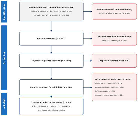
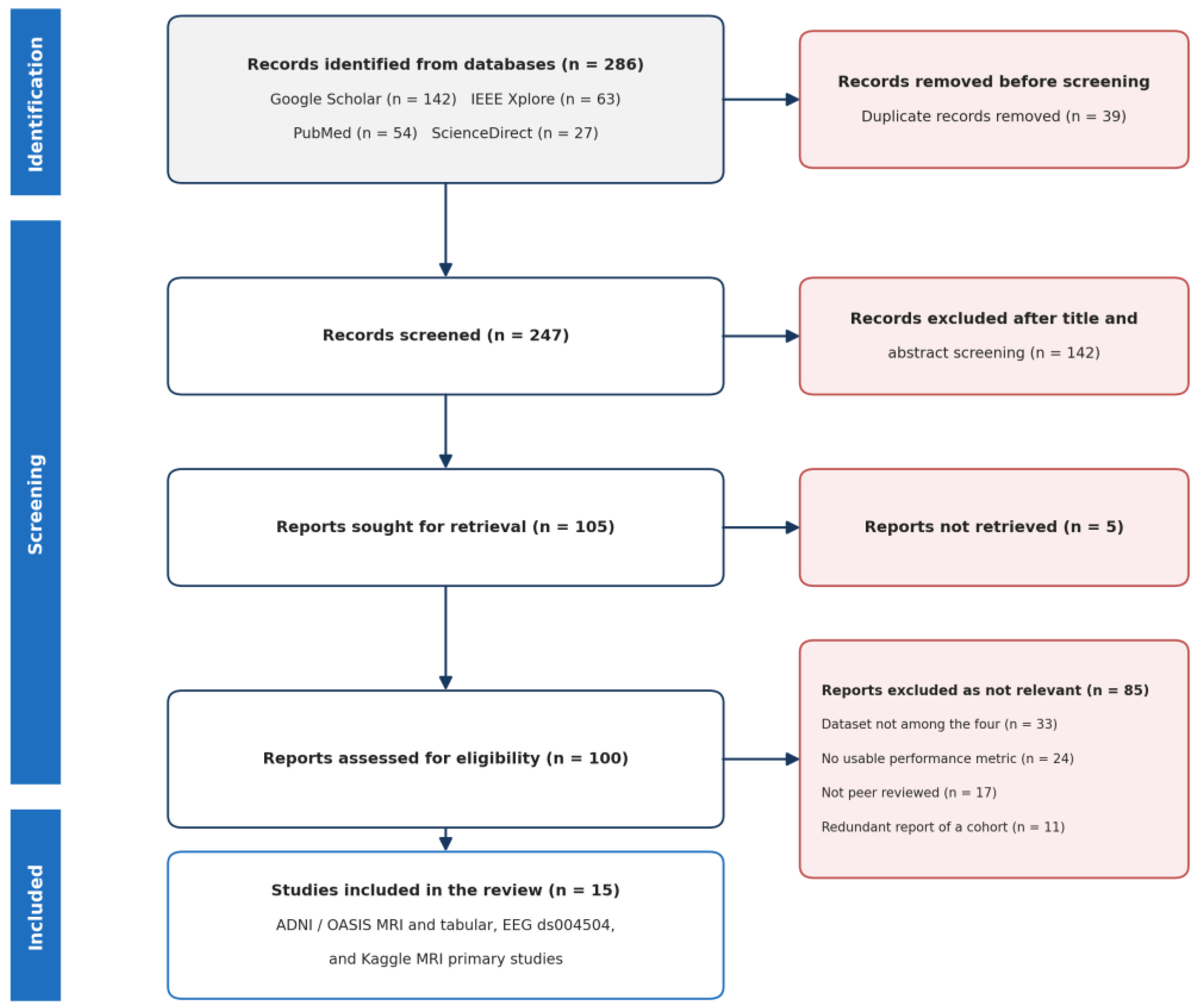
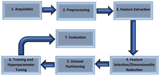
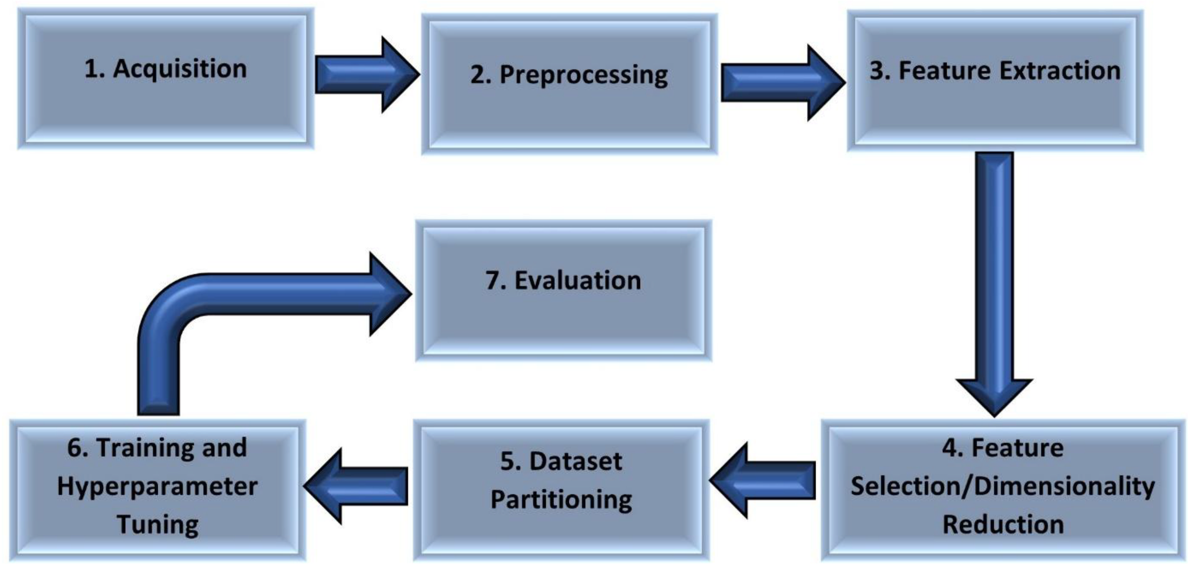
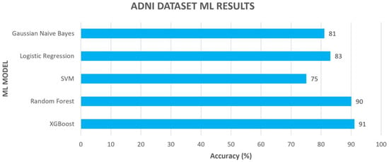
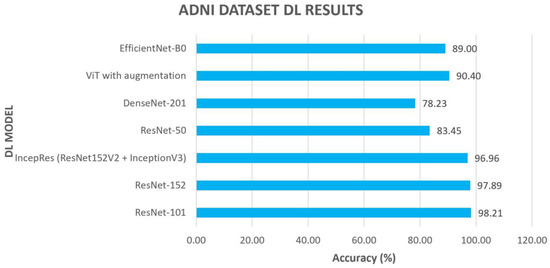
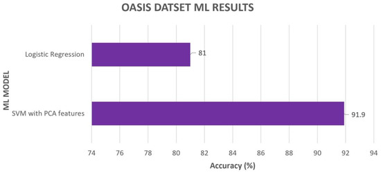
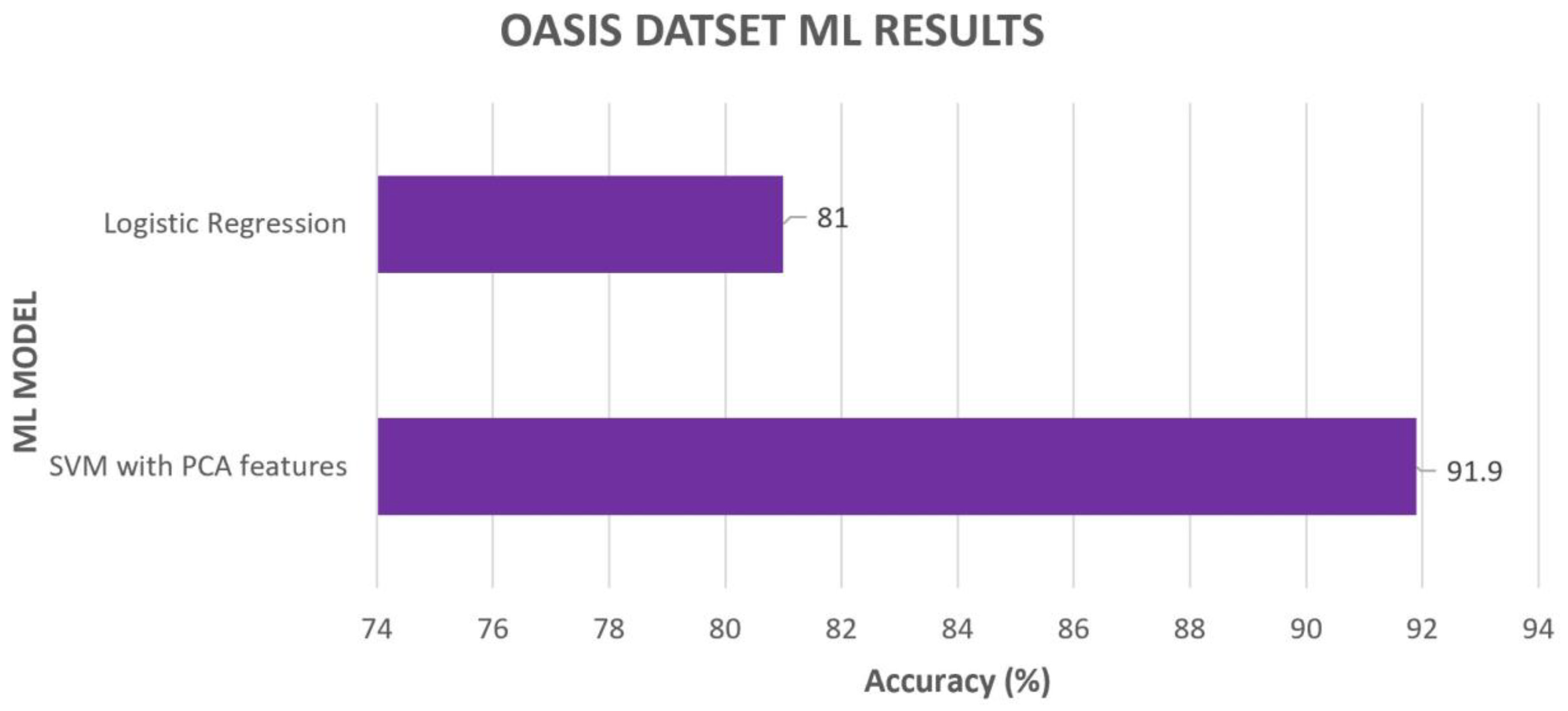
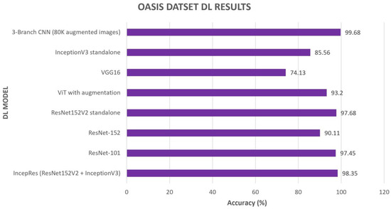
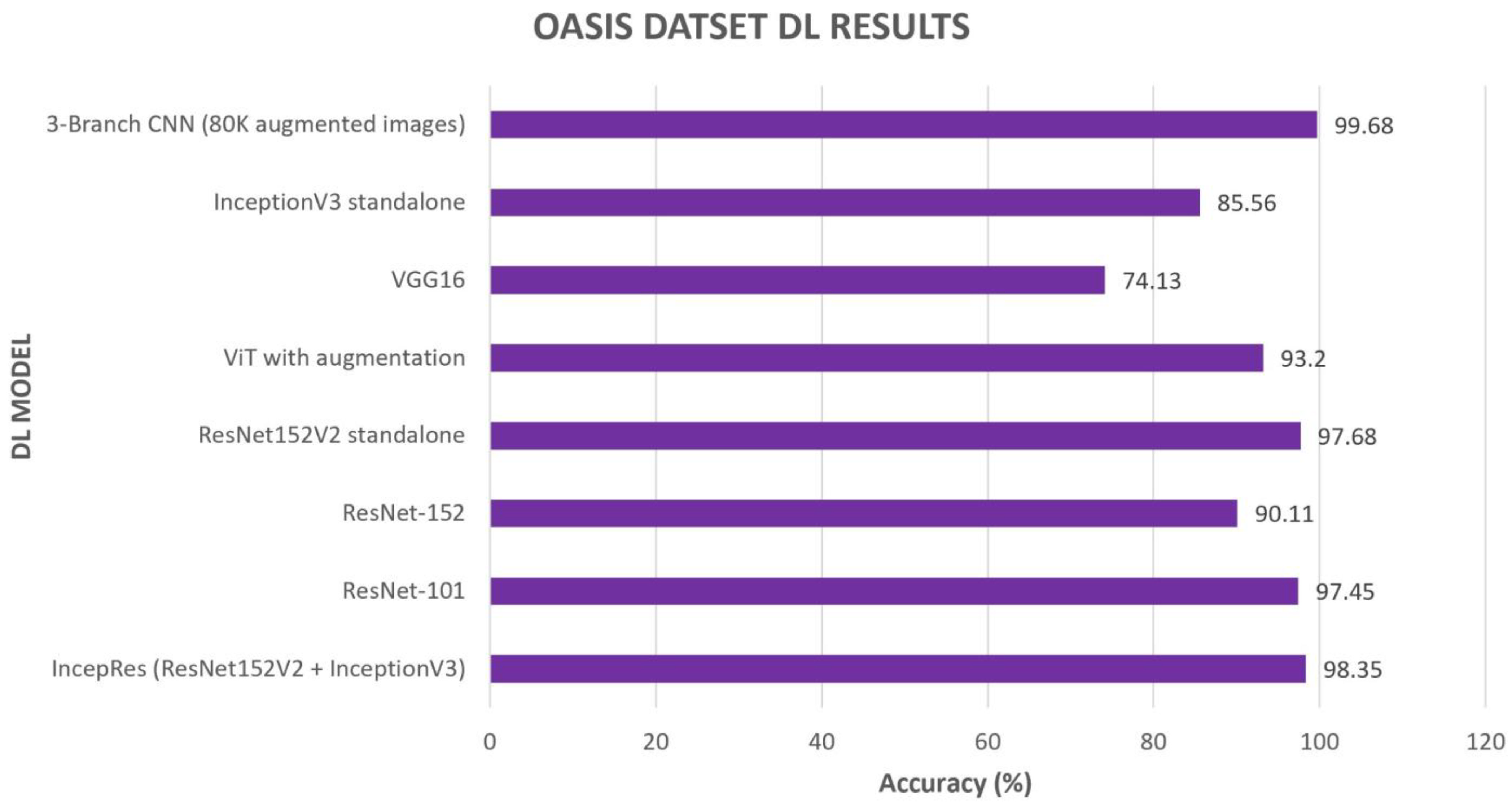
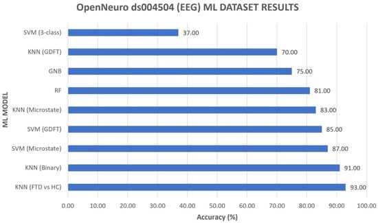
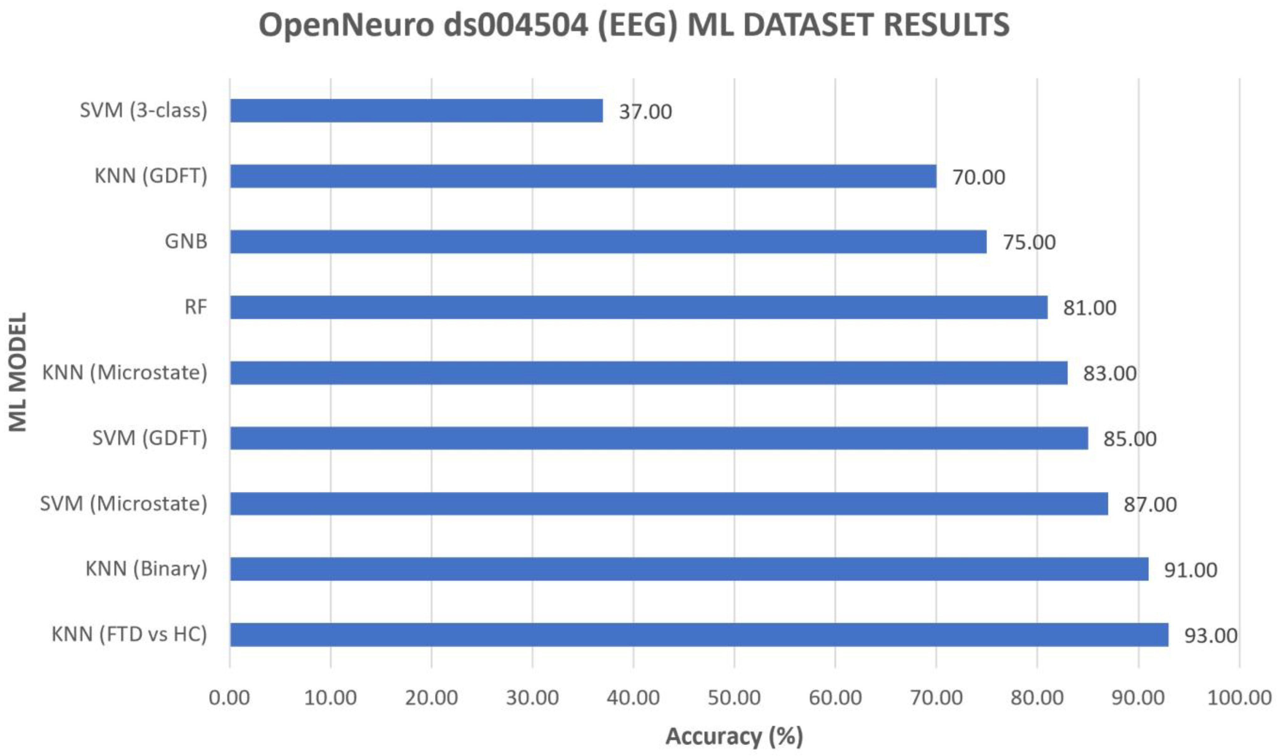
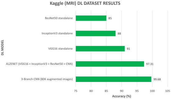
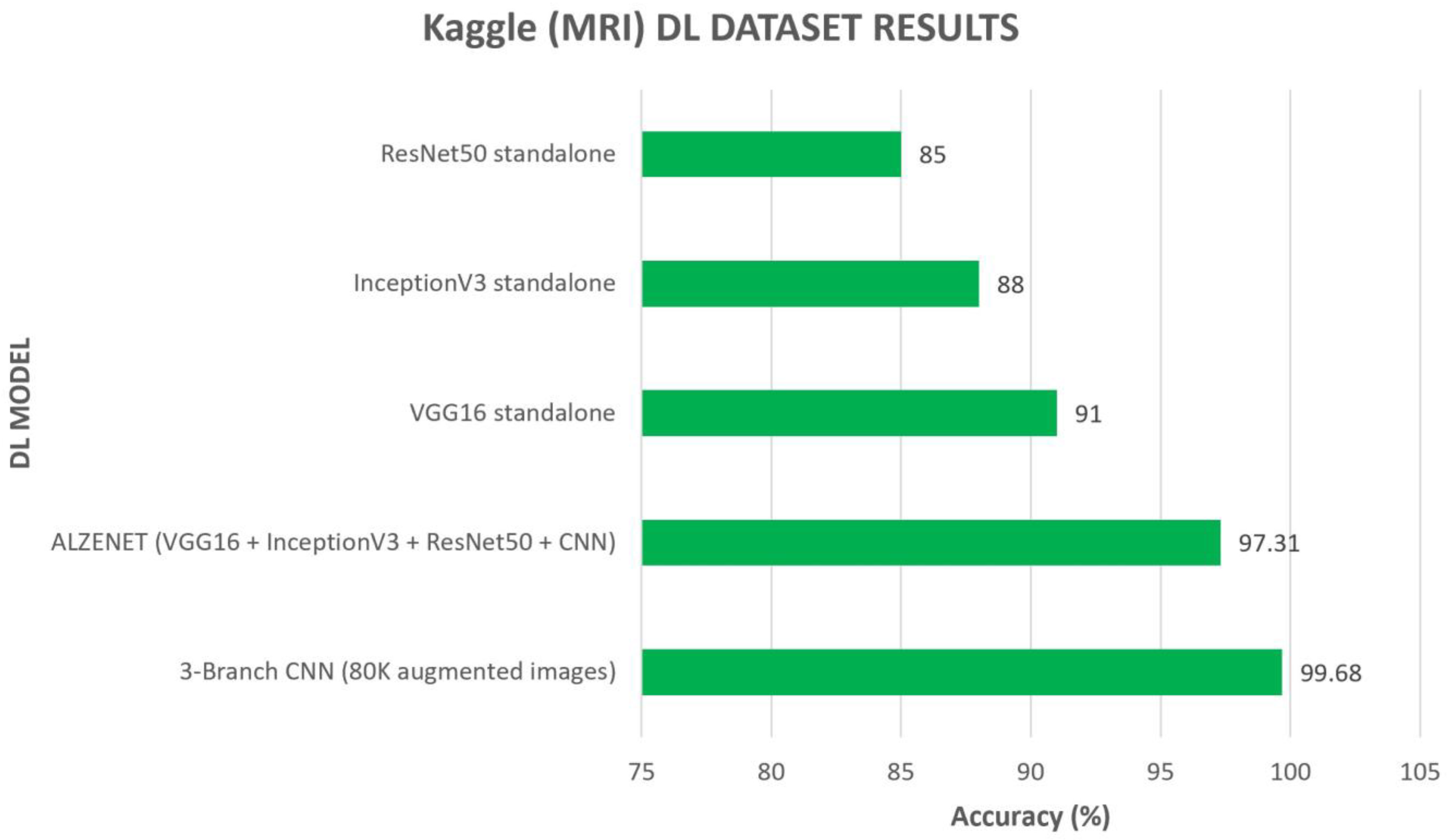
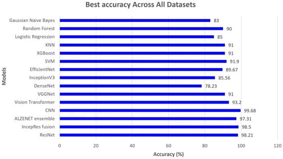

Disclaimer/Publisher’s Note: The statements, opinions and data contained in all publications are solely those of the individual author(s) and contributor(s) and not of MDPI and/or the editor(s). MDPI and/or the editor(s) disclaim responsibility for any injury to people or property resulting from any ideas, methods, instructions or products referred to in the content. |
© 2026 by the authors. Licensee MDPI, Basel, Switzerland. This article is an open access article distributed under the terms and conditions of the Creative Commons Attribution (CC BY) license.