


Abstract
Validating wireless power transfer (WPT) systems for electric vehicles (EVs) is a challenge due to efficiency variations caused by coil misalignments and height differences arising from various vehicle designs. Traditional simulation methods, such as finite element analysis (FEM), provide high accuracy but entail significant computational costs and calculation times, limiting the number of case studies and their optimization. This paper presents a methodology that integrates Machine Learning (ML) and Genetic Algorithms (GA) to overcome these limitations. An ML model rapidly and accurately predicts key electromagnetic parameters across a wide range of positions and frequencies. These predictions feed into a GA that optimizes control variables (voltages and frequency) with the objective of maximizing power transfer efficiency, while simultaneously ensuring component integrity at each operating point. Beyond drastically reducing simulation time and experimental effort, this methodology will enable knowledge extraction and its use for formulating design rules. These rules can lay the groundwork for developing simplified, real-time adaptive control strategies, facilitating the reduction of control variables and the narrowing of search ranges.
1. Introduction
Electric vehicles (EVs) are a key technology for advancing the decarbonization process. However, their adoption is hindered by several limitations, particularly the cost and range issues related to battery development and charging infrastructure. Inductive charging is the most promising, offering multiple advantages over conductive charging and battery swapping [1]. These advantages include ease of use, requiring no driver intervention, resilience against vandalism, and zero visual impact, making it especially appealing for city centers. In addition, it allows intermodal functionality, supporting static, opportunity, and dynamic charging modes. Lastly, it is fully interoperable, allowing any compatible vehicle to use the charging infrastructure.
Inductive charging fundamentally differs from conductive charging due to its reliance on magnetic coupling between coils [2,3,4,5], whose relative positioning varies with each charging event. This spatial dependence is absent in conductive systems, where a direct physical connection ensures consistent electrical contact. In the case of opportunity and dynamic wireless charging, misalignment between the transmitter and receiver coils can occur or evolve during the process. This introduces two main challenges: a more complex design [4,5,6,7] and a more sophisticated control strategy [5,7].
The SAE J2954 standard [8] seeks to standardize wireless charging systems by setting guidelines across several characteristics. These include a standard frequency range, specific height levels defined by three categories (Z1, Z2, and Z3), a maximum misalignment in the X and Y axes, and a minimum efficiency across all positions.
The design challenge has been studied extensively [2,4,7,9,10], but only [5] has presented a comprehensive methodology covering ferrite plate, shield, and a compensation circuit, ensuring system functionality in any charging position.
Regarding the control challenge, careful control of the primary voltage () and frequency (f), as well as the secondary voltage (), when feasible [5,6,7], is required. These must be adapted to the characteristics of the coils, their relative positioning, and the compensation circuit. The goal is to deliver the target power () with maximum efficiency, always ensuring that the maximum allowable current and voltage limits for each component of the transfer circuit are not exceeded [5,6].
Understanding the physical parameters of inductive coils and their shield in any position and at any frequency is essential. This is because the values of the primary coil’s self-inductance (), secondary coil’s self-inductance (), and mutual inductance (M) are influenced by the relative position of the coils [4,5,6,10,11]. The resistances of both windings ( and ) are also affected by the switching frequency [5,6,12,13,14].
From a modeling perspective, the challenge lies in addressing two different physical aspects: first, electromagnetic modeling to obtain inductor system parameters (, , M, , and ), and second, circuit modeling to derive optimal control variables (, and f), in order to achieve the desired power output () within the specified design constraints.
Several traditional approaches have been proposed for electromagnetic modeling.
- Analytical modeling [4,5,6,10]: This approach simplifies the system to an idealized formulation that neglects ferromagnetic materials and shield effects. In [6], analytical methods, finite element methods (FEM), and experimental results are compared. The findings show that analytical equations can achieve accuracy comparable to FEM results, with much lower computational cost. However, this approach is valid only for ideal configurations and does not capture inductance variations caused by displacement along the X, Y, and Z axes.
- Numerical Modeling: Several numerical techniques can be used to solve Maxwell’s equations [15], including the Finite Difference Method (FDM) [16,17], the Finite Volume Method (FVM) [18,19], The Integral equations Methods (IEM) [20], such as the Boundary Element Method (BEM) [21,22], and the Finite Element Method (FEM). Among these, FEM has been most widely adopted in inductive power transfer due to its ability to represent complex geometries, ferromagnetic materials, shield, and airgaps with high accuracy [5,12,14]. As noted in [6], FEM simulations can be computationally intensive. To mitigate this, simplifications such as 2D modeling for circular coils [23] or hybrid 2D/3D approaches for square coils with symmetric windings [7] are often employed.
Analytical methods are preferable when computational cost is critical, while numerical models offer higher accuracy at the expense of longer computation times. For circuit modeling, different approaches depend on the simulation objective and the available computation time.
In addition to traditional numerical simulations, various alternative approaches have been proposed in recent years to reduce the computational cost in electromagnetic modeling and system optimization. Among these, metamodeling techniques—which construct surrogate models from adaptive sampling—have demonstrated promising results for sensitivity analysis and rapid evaluation of complex systems [24,25]. These models, such as those based on Kriging or neural networks trained with efficient sampling, significantly reduce the number of necessary simulations while maintaining high accuracy [26].
Similarly, behavioral models, often based on simplified physical equations or parametric models, have been successfully used to characterize variations in mutual inductance in dynamic WPT systems [27]. These types of approaches have also been useful in quantifying uncertainty in the design of WPT systems [28].
These methodologies present clear advantages in terms of interpretability, lower data requirements, and low computational cost when applied to problems with moderate complexity or well-understood dynamics. However, they may show limitations when applied to scenarios of high dimensionality, strong non-linearity, or high spatial variability, as occurs in WPT systems operating in multiple positions and frequencies.
In this work, we adopt a machine learning-based approach, integrating neural networks with genetic algorithms, to efficiently model and optimize a WPT system. This choice is based on the superior capability of neural networks, in certain contexts, to capture complex non-linear relationships [29], generalize to unseen configurations [30], and easily couple with global optimization strategies, which allows reducing the dependence on detailed simulations without losing flexibility in modeling [31].
For circuit modeling, different approaches depend on the simulation objective and the available computation time.
- Steady-state analytical modeling [2,3,4,5,6,10,11,32]: This approach uses a first-harmonic approximation to solve the circuit in the phasor domain. It offers fast computation and an adequate representation of system performance, but it does not provide time-domain waveforms.
- Circuit numerical simulation [5,6,33]: Commercial circuit simulators such as LTspice, PSPICE, PSIM, or MATLAB-Simulink R2025b numerically solve the governing equations and generate time-domain waveforms of currents and voltages. This enables dynamic analysis and visualization, but it is typically more time-consuming.
- Differential equation analytical modeling [34,35]: In simple electronic systems (e.g., a series resonant circuit), closed-form solutions of the governing differential equations can be derived, providing waveform-level insights at low computational cost. However, this method is limited to systems with few components due to mathematical complexity.
When waveform acquisition is crucial and computation time is less critical, circuit numerical simulation is the most practical option thanks to its accessibility and visualization capabilities. Conversely, when computational efficiency is essential in complex systems, steady-state analytical modeling is more suitable, even if waveform detail is sacrificed.
In this context, analytical models are particularly advantageous for iterative optimization techniques, such as genetic algorithms (GA), due to their lower computational burden and straightforward integration into automated workflows. Numerical circuit simulations can also be integrated with GAs, as demonstrated in [36], but the higher per-iteration cost may become a limiting factor in large search spaces.
Several studies [2,3,4,10,37,38] have employed single-variable iterative search approaches (explicitly or implicitly) to tune control parameters. More recently, as highlighted in [5,6,7], multi-variable optimization using GAs has been proposed to determine optimal values for input voltage, output voltage, and frequency within the system’s operational limits.
As demonstrated, validating the complete system, including ferrite plates and shields, across all positions requires combining FEM modeling to calculate coil inductances and resistances with circuit modeling to resolve the circuit and derive control variables. This process is complicated by the frequency-dependent nature of resistances, necessitating FEM recalculations for each frequency at each position.
This paper builds upon the authors’ previous work. The first stage of this research line addressed an analytical design methodology for an S-S topology [6]. The second stage advanced to the complete optimal design of an SAE J2954-compliant WPT3 Z1 LCC-S system, including coils, ferrite plates, shielding, and compensation components, which was FEM-validated and experimentally tested at representative operating positions [5]. In contrast, the present work builds on that fixed physical design and addresses the subsequent step in the WPT design methodology: rapid operational validation and optimization of the control variables, namely the primary voltage Vp, secondary voltage Vs, and switching frequency f, across hundreds of misalignment and air-gap conditions using an ML-GA workflow.
The key innovation of this study is the shift from a static design perspective to a dynamic and operational one. We analyze the system’s behavior across a wide range of spatial misalignments (X, Y, Z), not just at a few discrete points. To achieve this, we introduce a novel methodology that integrates a Machine Learning (ML) model with a GA. This approach enables the rapid validation and optimization of control variables across hundreds of operating points, representing the culmination of the design process initiated in [5,6].
While the individual use of ML or GA in power systems is not new, the primary contribution of this work lies in their synergistic integration into a physics-informed and scalable framework for the validation and adaptive control of a complete, SAE J2954-compliant WPT system. In this framework, the FEM-trained NN acts as a fast surrogate electromagnetic model that is embedded inside the GA optimization loop.
Unlike prior studies that often focus on partial tasks, our methodology is comprehensive. First, it models all key electromagnetic parameters (, , M, , ), fully accounting for the effects of frequency, ferrite plates, and shields. Second, it includes an exhaustive comparison of eight ML algorithms to rigorously justify the selection of a Neural Network (NN) as the most efficient and accurate for this specific task (Section 5.3.2). Third, it evaluates the influence of the FEM-generated training-set size on prediction accuracy (Section 5.3.3). Finally, it integrates this fast NN model directly into a GA optimization loop to determine the optimal control variables (, , f) across 396 distinct misalignment and air-gap conditions. This methodology transforms a computationally expensive FEM-based point-by-point validation process into rapid adaptive control-map generation.
While this paper focuses on modeling and controlling the WPT physical layer, the resulting adaptive control map can be adapted for use in higher-level energy management. The ability to predict and optimize power transfer efficiency under any misalignment condition provides the foundational data needed for advanced, system-level strategies, such as those developed for microgrid energy management using deep reinforcement learning [39], fuzzy-PSO methods [40], or adaptive virtual impedance [41].
Therefore, our ‘bottom-up’, component-level optimization framework can be seen as a necessary building block to support the ‘top-down’, system-level management approaches explored in the broader literature [42,43,44].
Using these values and the equation-based circuit model, the GA seeks optimal control variable values (, , and f) for each position to achieve target power (), maximizing efficiency while adhering to voltage and current limits for all circuit components. This process iterates since , , and M depend only on position [5,11,12], while and also vary with frequency [5,6,12,13,14].
Selecting the most appropriate ML technique is essential, as the various methods in the literature exhibit performance variations depending on the applied system [45,46,47,48].
In recent years, the use of ML techniques in WPT systems has attracted increasing interest. Several studies have employed ML models for specific WPT-related tasks, including the prediction of system characteristics [49], mutual inductance or coupling-related quantities [50,51], parameter identification and sensorless receiver-characteristic estimation [52,53], receiver-position estimation [54], parameter optimization [55], and long-range WPT applications [56].
However, most of these contributions focus on partial tasks, without simultaneously integrating electromagnetic modeling, circuit modeling, and control optimization. Moreover, none of these works provide a systematic evaluation of the relative performance among different ML algorithms, nor explicitly address dataset size requirements or input preprocessing needs.
In this work, we propose an automated methodology that combines an ML model based on a neural network (NN) to estimate electromagnetic parameters (, , M, , ) as functions of frequency, position, and misalignment, together with an equation-based circuit model and a GA for control optimization. This approach not only validates the operation of previously designed WPT systems but also enables rapid performance evaluation across a broad range of scenarios, complying with the SAE J2954 standard and suitable for integration into dynamic or opportunistic charging systems.
As a key additional contribution, this paper provides a comprehensive comparison among ML algorithms (Linear Regression, k-NN, linear and nonlinear SVM, Random Forest, Gradient Boosting, XGBoost, and Neural Networks), analyzing their accuracy, robustness, and data volume requirements to achieve acceptable performance. This analysis is complemented with correlation studies among variables and optimal preprocessing schemes, allowing selection of both relevant variables and the most efficient model. It is demonstrated that neural networks provide the highest accuracy while requiring fewer data samples for adequate training.
The table-based approach can be implemented by detecting relative coil positions or calculating electromagnetic circuit parameters. Lookup table-based controls could be invaluable in dynamic and opportunity charging scenarios, minimizing control convergence time and optimizing performance—an especially critical factor given the limited charging time available.
Although the present study is based on offline modeling and simulation, the framework developed herein lays a solid foundation for future onboard integration. By incorporating real-time sensor data and adaptive control strategies in subsequent developments, this methodology could evolve into a dynamic digital control system for EV charging, capable of continuously adjusting parameters in response to varying operating conditions.
The proposed method applies to any WPT topology. In this study, it is applied to an LCC-S WPT3Z1 system previously designed in [5]. The LCC compensation topology is chosen for the primary side because it is one of the example configurations illustrated (but not mandated) in SAE J2954 standard [8], and compared to other topologies, it offers the following advantages:
- Improved efficiency over simpler topologies [3,57].
- Greater misalignment tolerance [2,3].
- Reduced inverter current and its variability compared to topologies like S-S [2].
The document is structured as follows: Section 2 introduces the WPT3 Z1 LCC-S system parameters designed in [5] and utilized in this study. Section 3 summarizes the steady-state circuit model used to calculate the delivered power and evaluate the electrical constraints in the GA. Section 4 describes the 3D FEM-based procedure used to generate the electromagnetic dataset, including , , M, , and , for training and validating the ML algorithms. Section 5 discusses the ML algorithms employed for comparative analysis. Section 6 outlines the GA implemented, integrating the selected ML model with the model from Section 3. Section 7 presents the modeling results obtained with the ML algorithm and with the GA. In contrast, in Section 8, the results of the ML model are compared with those obtained from 3D FEM and with experimentally obtained values. Additionally, the results achieved by the GA are compared with those produced by MATLAB-Simulink and those obtained from an experimental test bench.
In this paper, parameters related to the primary side are denoted with the subscript ‘p’ (e.g., for the number of turns in the primary coil), while those for the secondary side use the subscript ‘s’ (e.g., for the number of turns in the secondary coil). When a parameter applies to both sides simultaneously, we use the subscript ‘ps’ (e.g., represents the total number of turns shared by both coils).
2. WPT3Z1 LCC-S Parameters
The SAE J2954 standard [8] focuses on ensuring the interoperability, safety, and efficiency of WPT systems, addressing key aspects such as electromagnetic compatibility, positioning, communication protocols, and energy transfer performance. It defines categories by both power levels and ground clearance ranges. Regarding power, the WPT is divided into three categories based on Input Volt-Amps (VA): WPT1 up to 3.7 kVA, WPT2 up to 7.7 kVA, and WPT3 up to 11.1 kVA [58]. Regarding ground clearance ranges, the standard specifies two distinct classifications. Firstly, VA Coil Z-classes define the vertical distance between the ground surface and the lower surface of the VA coil package (vehicle-side coil), with categories Z1 from 100 to 150 mm, Z2 from 140 to 210 mm, and Z3 from 170 to 250 mm [58]. Secondly, Ground Assembly (GA) Z-classes specify the range of VA coil ground clearances over which a GA test station or product operates, aiming for interoperability. For these GA Z-classes, the categories are Z1 from 100 to 150 mm, Z2 from 100 to 210 mm, and Z3 from 100 to 250 mm, noting that all GA Z-classes share a common lower limit of 100 mm to ensure broader compatibility. These power and ground clearance categories can be combined in various ways to accommodate different vehicle and charging needs. For instance, WPT3 Z1 (referring to VA Coil Z-class) denotes a power transfer of up to 11.1 kVA with VA coil ground clearance distances from 100 to 150 mm.
The LCC-S topology [2,3,5] is an enhanced hybrid resonant circuit configuration used in WPT systems. It effectively combines features from both series-series (S-S) and parallel-series (P-S) topologies, offering improved performance characteristics compared to these basic configurations. The topology includes two primary compensation capacitors: , connected in series, and , connected in parallel. By adjusting the values of these capacitors, the system can behave more like either the S-S or P-S topology, enhancing performance in response to changes in position and battery voltage. To ensure compatible switching conditions, an auxiliary inductor is included, preventing direct inverter commutation over the capacitive input of the resonant network. On the secondary side, series compensation ensures that the reflected impedance has only a real component, simplifying the calculation of the primary capacitors and reducing the number of required passive components.
Table 1 defines the fixed parameters established by the Standard for the case of WPT 3 Z1 with rectangular coils.
Table 1.
Fixed parameters according to a WPT3 Z1 from SAE J2954 Z1 [8].
This study builds upon a specific WPT3 LCC-S system, whose compensation topology (LCC-S), coil geometries, and initial design parameters were thoroughly developed and optimized in our previous work [5]. This “WPT-designed system” was configured to meet the SAE J2954 WPT3 power class requirements (up to 11.1 kVA) and standard-defined external coil dimensions. For the purpose of this paper, which focuses on power delivery management, we utilize the established physical design of this system as a fixed operational platform. Therefore, coil dimensions, ferrite plates, shielding, and compensation components are not re-optimized here; only the operating control variables are optimized for the admissible misalignment and air-gap conditions.
Table 2 presents the key geometrical and electrical parameters of this reference WPT3 LCC-S system. These parameters, including the most critical coil dimensions, number of turns, and total wire cross-section, define the physical characteristics of the system used throughout our analysis.
Table 2.
Most important dimensions of the WPT designed system, number of turns, and total cross-section.
Where a is the width and b is the outer length of the primary and secondary coil, and are the outer width and length of the ferrite layer; S refers to the cross-sectional area of the conductors, and N is the number of turns.
Table 3 shows the values of the inductances , , and M of the coils in the nominal position, as well as the values of the compensation circuit.
Table 3.
Values of the inductances in nominal position and values of the compensation circuit.
3. Circuit Modeling and Final Expression for Delivered Power
The steady-state circuit model follows the first-harmonic phasor formulation commonly used for resonant WPT systems [4,5,6,10]. Since the WPT system has already been designed, the model is not used here to re-size the compensation network, but to evaluate the delivered power and the electrical constraints for each set of control variables.
The system is divided into two sides, as shown in Figure 1 of [5]:
The battery and rectifier stage are represented by an equivalent load resistance:
where is the controlled secondary-side voltage and is the target delivered power. The secondary-side impedance is:
And the reflected impedance is:
The equivalent primary-side impedance seen by the primary coil branch is therefore:
Considering the LCC-S compensation network, the primary-coil current can be expressed as:
And the secondary current is:
Thus, the power delivered to the equivalent load is:
Or, equivalently,
where the magnitude of the secondary impedance is:
Equation (8) gives as a function of the control variables and the impedances and . Equation (9) expands , while Equation (4) defines , which includes the primary impedance and the impedance reflected from the secondary side. Therefore, the power actually delivered to the load depends on four sets of parameters in addition to the target power :
- Fixed circuit parameters: , , , and .
- Position-dependent electromagnetic parameters: , , and M.
- Position- and frequency-dependent electromagnetic parameters: and .
- Operating control variables: , , and f.
The values of the capacitors are previously defined, as well as those of the inductances, although the latter are for the nominal position, as shown in Table 2. However, since the charging process can occur in any position and height according to SAE J2954 (Table 1), the values of the inductance and resistances are modified; the latter are also affected by the working frequency. This is why they must be modeled using finite elements, as explained in the following section.
As for the variable parameters to be controlled, maximum and minimum values are also defined in Table 4.
Table 4.
Maximum and minimum values of the control variables.
4. Electromagnetic Model
The ML models require a supervised dataset containing the electromagnetic parameters of the complete WPT system, namely , , M, , and . These parameters could be estimated using analytical expressions, as commonly done in simplified WPT models [4,5,6,10]. However, analytical formulations usually neglect the influence of ferrite plates, aluminum shields, and the vehicle mimic plate, and therefore cannot accurately reproduce the electromagnetic behavior of the complete SAE J2954-compliant inductor system. For this reason, the dataset used in this work was generated using 3D FEM simulations in COMSOL Multiphysics 6.2.
The FEM model reproduces the test platform defined in SAE J2954 [8] and previously used in [5], including the primary and secondary coils, ferrite plates, aluminum shields, and the vehicle mimic plate. The extraction of self-inductances and mutual inductance follows the standard frequency-domain FEM procedure described in [5,11,14,33]. In this approach, the self-inductance of each coil is obtained from the imaginary part of the ratio between the induced voltage and the imposed current, whereas the mutual inductance is obtained from the induced voltage in one coil due to the current imposed in the other coil. Therefore, , , and M are mainly governed by the relative position between the primary and secondary coils, including lateral misalignment and vertical air gap.
The equivalent AC resistances and were also obtained from the FEM model. Unlike the inductances, these resistances depend not only on the geometry and relative coil position, but also on the operating frequency because of skin and proximity effects in the windings [5,6,12,13,14,33,59]. These effects are especially relevant in the frequency range considered for SAE J2954 WPT systems. Consequently, Litz wire is used to reduce AC losses, as recommended in previous studies [5,6,12,13,14,33,59,60,61]. The strand diameter selected in the reference design is 0.1 mm, which is suitable for the operating frequency range [60], and a packing factor of 0.5 is considered for the total conductor cross-section [61].
Since the GA optimizes the switching frequency (f), assuming constant resistance values would introduce errors in the calculation of losses, efficiency, and component constraints. Therefore, and were computed for each FEM case at the corresponding frequency, whereas , , and M were associated with the corresponding spatial configuration. The FEM simulations were thus carried out over the admissible range of lateral misalignment, air gap, and frequency. The resulting values of , , M, , and constitute the dataset used in Section 5 to train and validate the ML models.
5. Selection of the Machine Learning Technique for Electromagnetic Modeling
As outlined in this paper, the goal is to develop an automated and efficient method for designing and validating control systems under varying relative positions between coils, in accordance with the framework established by the SAE J2954 Standard. This necessitates the rapid calculation of inductance and resistance values (, , M, , ) for any given misalignment position (, , ) and frequency () quickly and without requiring intervention from the designer. So that they can be included in an iterative calculation process or, as in this paper, in a GA. For this reason, data-based models or ML models are employed.
Data-based models can be broadly categorized into Supervised and Unsupervised learning [45].
- Supervised learning involves creating a model or extracting knowledge by training it on a dataset where the inputs (features) and their corresponding outputs (labels or target values) are known. This approach is helpful for problems where the relationship between input and output is well-defined.
- Unsupervised learning, in contrast, analyzes data without prior knowledge of the labels or target values and does not have access to the expected outcomes. This technique is used to uncover hidden patterns or structures within the data.
Supervised learning is particularly relevant for our application, as the objective is to predict the outcomes based on a set of input variables. Supervised learning algorithms can be further divided into Classification and Regression [45,46,47,48]:
- Classification algorithms are used to predict outcomes in discrete categories or classes.
- Regression algorithms are used to predict continuous outcomes.
Since we work with known examples and the system’s behavior exhibits continuous variation, we will apply supervised learning using regression models. It is important to note that, in this case, the goal is to predict the values of five independent variables. Consequently, the study will be conducted for each variable individually, ensuring accurate prediction for each.
Given the diversity of ML modeling techniques and their varying suitability across different applications, it is crucial to explore multiple methods to identify the most effective approach for the specific problem [45,46,47,48]. The techniques selected for analysis in this study include Linear Regression, K-Nearest Neighbors (KNN), Support Vector Machines (SVM), Non-Linear SVM, Random Forest, Gradient Boosting, Extreme Gradient Boosting (XGBoost), and Neural Networks. These algorithms represent diverse methods commonly employed in ML tasks due to their versatility and demonstrated success in various domains [45,46,47,48].
A key factor in optimizing the performance of these algorithms is the careful adjustment of hyperparameters. Hyperparameters are settings that dictate how a model learns from data, influencing the algorithm’s complexity and behavior. Unlike model parameters, which are learned from the training data (such as weights in a regression model or support vectors in SVM), hyperparameters are set before the training process begins and must be fine-tuned to achieve optimal performance [45,46,47,48].
Hyperparameter tuning is essential, as it can significantly affect the model’s accuracy, generalization ability, and capacity to handle new, unseen data. Practical tuning involves a systematic search for the best hyperparameter configurations, typically utilizing techniques such as grid search, random search, or more advanced optimization methods [45,46,47,48].
5.1. Explanation of Models and Hyperparameter Selection
5.1.1. Linear Regression (LR)
This ML model predicts the target variable through a linear combination of the predictor variables . The relationship can be expressed in matrix form as seen in Equation (10):
where corresponds to each target variable to be predicted (, , M, , ). The term (, , , ) represents the weight vector, with the value of = 0 in the case of inductances.
The term corresponds to the bias term of the model for each variable to be predicted, while denotes the prediction error.
The model fitting involves obtaining the weights and the bias term in such a way that minimizes the mean squared error of the model’s predictions using least squares (Equation (11)) [62]:
where n is the total number of samples in the training dataset.
5.1.2. k-Nearest Neighbors (K-NN)
The k-Nearest Neighbors (K-NN) algorithm is a ML algorithm that utilizes the concept of proximity to make predictions about a new data point. This algorithm can be used for both classification and regression tasks. In the case under study, the predicted value is obtained by averaging the K nearest points from the training data. Therefore, it is crucial for its effective performance that the training samples are representative and homogeneous throughout the prediction space [45,48,63].
In this context, we have selected K-NN because the training data have been generated using random functions that ensure the homogeneity of the points in the feature space, which is suitable for this method. The prediction can be defined as shown in Equation (12) [64].
where are the weights that define the influence of each neighbor, and j corresponds to the variable to be predicted , , M, , .
In this case, the hyperparameter to identify is K, which defines how many nearest neighbors are considered for making the prediction.
5.1.3. Support Vector Machines (SVM)
Support Vector Machines (SVM) are algorithms for classification and regression tasks. This methodology is based on defining hyperplanes that, in the case of classification, separate different classes and, in the case of regression, enable the prediction of target values.
SVM shares similarities with linear regression, with the primary difference being the objective function. In linear regression, the goal is to determine the weights that minimize the sum of squared errors. For SVM, the acceptable error is introduced as a constraint within the optimization problem, while the objective function focuses on minimizing the norm of the weights. The problem is formally defined as follows [45,48,64]:
This formulation creates an optimization problem solved using the gradient descent method, where the error constraint is crucial to mitigating overfitting.
Nevertheless, this algorithm encounters some challenges. Even after solving the objective function, specific data points may lie outside the established error margins. A slack variable () addresses this, representing the distance between the actual value and the allowable error margin.
Consequently, the objective function and constraints are redefined as follows [64]:
In this algorithm, the hyperparameters to optimize are:
- C, which controls the penalty for misclassified points or points with errors in regression.
- , which defines the acceptable error margin in the regression predictions.
5.1.4. Non-Linear SVM
The Non-Linear SVM algorithm was developed for scenarios where classification or regression cannot be achieved using linear methods. In such cases, the methodology focuses on achieving non-linear regression by expanding the dimensions of the original feature space [64].
In this study, several kernel functions are explored, including Radial Basis Function (RBF), Polynomial (of degrees 2 to 5), Sigmoid, and Linear. The RBF kernel is used as an example and is mathematically defined as follows [64]:
Here, the parameter governs the behavior of the kernel function. When is small, the system resembles a Linear SVM, as the decision boundary becomes simpler and linear. As increases, the model’s flexibility increases, enabling it to capture more complex patterns and create a more intricate decision boundary.
The hyperparameters to optimize in this case are:
- : Defines the acceptable margin of error for predictions in regression tasks. Larger values tolerate more error, while smaller values aim for greater precision.
- : Determines the shape and flexibility of the RBF kernel, impacting the model’s ability to generalize complex patterns.
- C: The regularization parameter balances the trade-off between minimizing training error and maintaining model complexity to avoid overfitting.
5.1.5. Random Forest (RF)
A Random Forest model consists of an ensemble of individual decision trees, each trained on a different data sample obtained through bootstrapping. This approach offers flexibility, as the final prediction is computed as the average of the results from all the trees, unlike other regression models that rely on a single predictive equation [45,46,47,48,65].
The hyperparameters considered for this model include [46,65]:
- Maximum Number of Estimators: Specifies the total number of trees in the forest.
- Feature Subsampling: Controls the number of features considered at each split.
- Maximum Tree Depth: Limits the depth of individual trees to prevent overfitting.
- Minimum Samples to Split a Node: Specifies the minimum number of samples required to split a node in each tree.
- Minimum Sample Size for New Splits: Indicates the number of data points needed to create a new tree.
5.1.6. Gradient Boosting (GB)
The Gradient Boosting method builds models sequentially using decision trees. In each iteration, the algorithm focuses on correcting the errors made by the model in the previous iteration, progressively improving accuracy [45,46,47,48,65,66].
The hyperparameters of this algorithm include [46,66]:
- Maximum Number of Estimators: Specifies the total number of trees in the model.
- Learning Rate: Controls the contribution of each tree to the final model.
- Maximum Tree Depth: Limits the depth of individual trees to prevent overfitting.
- Minimum Samples to Split a Node: Specifies the minimum number of samples required to split a node in each tree.
- Minimum Sample Size for New Splits: Indicates the number of data points needed to create a new tree.
5.1.7. Extreme Gradient Boosting (XGBoost)
XGBoost is a tree-based boosting algorithm that enhances model performance using gradient optimization and advanced regularization techniques. Unlike other boosting algorithms, XGBoost stands out for its ability to handle large datasets and high computational efficiency, making it one of the most widely used algorithms in ML competitions. During training, XGBoost iteratively adjusts the errors made by previous trees, focusing on minimizing the loss function [45,46,47,48,67]. In this work, the XGBoost regression model was implemented using XGBoost v3.1.3.
The hyperparameters of this model include [46,67]:
- Number of Estimators: Specifies the total number of trees used in the model.
- Learning Rate: Controls the contribution of each tree to the final model.
- Maximum Tree Depth: Limits the depth of individual trees to prevent overfitting.
- Subsampling: Defines the fraction of samples used to train each tree, which can help improve generalization.
- Regularization (L1/L2): Adds penalties to the model to prevent overfitting.
- Tree Growth Rate: Specifies the speed at which trees are constructed in the model.
5.1.8. Neural Networks (NN)
Neural networks are composed of interconnected nodes that perform simple mathematical operations across successive layers: input, hidden, and output. During training, weights and biases are optimized to minimize the difference between predictions and actual values. In this case, we utilize deep neural networks (DNNs), with an input layer corresponding to the number of predictor variables and an output layer containing a single neuron for the target variable. Between these layers, there are hidden layers with an equal number of neurons. One of the key advantages of these models is their ability to perform regression on multiple variables using a single model [45,46,47,48,68,69].
The hyperparameters for this case are [68]:
- Number of Hidden Layers: Determines how many hidden layers will be included in the network.
- Number of Neurons per Layer: Specifies the number of neurons in each hidden layer.
- Learning Rate: Controls the magnitude of adjustments to weights and biases during training.
- Activation Function: Specifies how neurons are activated in the hidden and output layers (e.g., ReLU, Sigmoid).
- Batch Size: Indicates how many samples are processed before updating the weights.
- Number of Epochs: Defines how often the model trains on the entire dataset.
- Regularization: Applies techniques (e.g., L1 or L2) to prevent overfitting by adding a penalty to the cost function.
- Dropout Rate: Specifies the proportion of neurons that will be randomly deactivated during training to prevent overfitting.
5.2. Data Preparation
This phase involves obtaining the data to train ML models. Once collected, the data must be normalized, and subsets are selected to train the models and validate their results. Traditionally, data for training are acquired experimentally. However, in this study, given that it is in the design phase, we propose a data acquisition method based on electromagnetic models obtained using the Finite Element Method (FEM). The selection of the training dataset is a critical step. The input space is four-dimensional (, , , f), and each FEM simulation has a high computational cost. Therefore, the dataset must be sufficiently representative of the operating region but small enough to keep the data generation feasible.
To determine the optimal number of samples, we performed a convergence analysis, as detailed in Section 5.3.3. As shown in Figure 1, the model’s performance (measured by R2 and RMSE) stabilizes significantly after approximately 30–40 training samples, indicating that further increases in data yield diminishing returns.
Figure 1.
Evolution of R2 and RMSE as a function of the number of cases for Gradient Boosting (top row) and Neural Networks (bottom row) when estimating .
Based on this analysis, we chose to generate 100 cases. This number provides a robust safety margin to ensure the model is well-trained and generalizes effectively, without incurring an excessive computational cost.
Crucially, these 100 cases were generated using random values to ensure a homogeneous distribution throughout the feature space, which is vital for the model to accurately capture the system’s non-linearities. The specific ranges are defined as follows:
This vector, , is simulated using the commercial tool COMSOL Multiphysics, which yields the values of , , M, , . Consequently, a new vector Y is obtained for each X, represented as:
Here, refers to and , while refers to and .
5.2.1. Data Correlation Analysis
In line with [69,70], a correlation analysis was performed to evaluate how variations in one variable influence the others and to quantify the strength of these relationships. The results of this analysis are presented in Figure 2, which shows a comprehensive correlation matrix. This matrix integrates histograms on the main diagonal, scatter plots in the lower triangular section, and Pearson correlation coefficients in the upper triangular section, enabling both visual and quantitative interpretation of intervariable relationships.
Figure 2.
Correlation matrix among the main parameters involved in the inductive link. The diagonal shows histograms of each variable’s distribution. The lower triangle contains scatter plots for each pair of variables, while the upper triangle displays the Pearson correlation coefficient in a visual format.
Each circle in the upper triangle of the matrix represents the Pearson correlation coefficient between a pair of variables. The size and color of the circle encode the magnitude and sign of the linear correlation, respectively: larger circles correspond to stronger correlations (positive or negative), while smaller circles reflect weaker or negligible correlations. The color indicates the direction of the relationship: red represents a positive correlation (i.e., both variables increase or decrease together), while blue indicates a negative correlation (i.e., one variable increases as the other decreases). Values near +1 or −1 imply strong linear relationships, while values near 0 indicate weak or no linear dependence.
Several relevant relationships emerge from this analysis. As expected from theoretical models [5,11,12,33], the mutual inductance (M) and the primary inductance () exhibit no significant correlation with the operating frequency. This is evident in the scatter plot at column 4 (), row 7 (M), where the data points show a wide dispersion with a flat trend over the 80–90 kHz frequency range, indicating that M remains approximately constant. This observation is confirmed by the Pearson coefficient in column 7 (M), row 4 (), which shows a very small circle, indicating a negligible correlation value.
In contrast, a strong positive correlation is observed between frequency () and the power loss resistance (), consistent with previously reported behaviors in inductive power transfer systems [5,6,13,14,33]. The scatter plot at column 4 (), row 8 () shows a clear increasing trend: as the frequency increases from 80 to 90 kHz, Rps rises from approximately 0.175 Ω to 0.2 Ω. The strong linear clustering is confirmed by the Pearson coefficient in column 8 (), row 4 (), which reaches 0.90, represented by a large red circle, indicating a strong and positive linear relationship.
Spatial alignment between the coils also proves critical: both (secondary inductance) and M show clear dependence on the relative coil positions. A particularly strong negative correlation is found between Ls and the vertical misalignment variable (). In the scatter plot at column 1 (), row 6 (), the points are tightly clustered along a decreasing curve, showing that drops from about 200 μH to 180 μH as increases. This result is consistent with the expected degradation of magnetic coupling due to increased coil separation. The Pearson coefficient in column 6 (), row 1 () is –0.99, indicated by a large blue circle, implying an almost perfect negative linear relationship.
These findings are particularly relevant for the design of ML models. The presence or absence of strong correlations helps to guide feature selection, allowing the exclusion of irrelevant or redundant variables. For example, frequency can be omitted when predicting and M, but it must be retained when predicting . Conversely, geometric misalignments like are essential for predicting magnetic coupling parameters such as and M.
As a result of the correlation analysis, developing ML models will be simplified by excluding the frequency variable when predicting and M. However, the frequency variable will still be considered for predicting .
5.2.2. Data Standardization
ML algorithms are generally sensitive to the scaling of data. For example, in Neural Networks, Linear Regression, or K-Nearest Neighbors, differences in scale or variance between variables can result in varying coefficient values and lead to outputs that deviate from expected values for certain inputs; this effect can be more pronounced in cases of small datasets such as ours [71]. However, this issue does not affect algorithms based on decision trees, making variable scaling unnecessary for those methods [65,66,67,71,72].
In this study, the variable have values in the range of hundreds of millimeters, while frequency values range between 79 and 90 kHz. This disparity necessitates data scaling.
Different normalization techniques are recommended depending on the type of ML algorithm used and the data’s characteristics. The preprocessing methods applied for each algorithm are summarized in Table 5:
Table 5.
Preprocessing Method for Each Algorithm.
Min-Max Normalization
To normalize the data using the Min-Max method, Equation (18) is applied:
where j corresponds to the predictor variables, represents the new scaled values, are the unscaled values, is the minimum value in the dataset , and is the maximum value in .
Min-Max normalization is particularly useful when data need to be compared on a consistent, fixed scale. For instance, this technique benefits algorithms that compute distances (e.g., K-Nearest Neighbors) or neural networks. It ensures input values are within a known, constant range, which can improve the convergence of certain optimization algorithms.
Standardization (Z-Score Normalization)
This method transforms feature values in a dataset so they have a mean of zero and a standard deviation of one. This is achieved by subtracting the mean of the data and dividing the result by the standard deviation (Equation (19)):
Z-Score normalization is beneficial because it compares features with different units and value ranges within the same dataset. Furthermore, this method’s normalized data are more robust to outliers than other normalization techniques.
5.3. Modeling and Validation
5.3.1. Validation Metrics: and
The metrics (Equation (21)) and (Equation (22)) will be used to compare the results obtained from each ML algorithm [45,46,47,48,69].
For , values closer to one indicate better performance, while for RMSE, lower values closer to zero signify better results.
The combination of and RMSE provides a robust model performance evaluation. While indicates the proportion of variance explained by the model, with higher values reflecting a better fit, RMSE offers a direct measure of prediction error. Lower RMSE values indicate better accuracy, while the quadratic nature of RMSE ensures that larger errors are penalized more heavily. This characteristic makes RMSE particularly useful for identifying models that might be over-predicting or under-predicting extreme values. Together, these metrics provide a comprehensive assessment, considering both the goodness of fit and the model’s sensitivity to large prediction errors, offering a balanced evaluation of the ML algorithms under consideration.
5.3.2. Validation and Selection of the Most Suitable Modeling Technique
A global performance comparison of the algorithms was performed by calculating the mean and standard deviation for both and RMSE. The evaluation was conducted on a dataset divided into 75 training samples and 25 test samples. The and RMSE values for each algorithm are reported in Table 6 and Table 7, respectively.
Table 6.
Obtained Across Different Models.
Table 7.
RMSE Obtained Across Different Models.
To complement these numerical results, Figure 3 provides a visual comparison of the algorithms. In the upper part of Figure 3, the performance is displayed along with error bars representing the standard deviation, which allows for quick identification of models with a good overall fit. The lower part of Figure 3 illustrates the RMSE values and their variability, offering insights into the accuracy and consistency of the predictions.
Figure 3.
Performance comparison between algorithms.
As shown in Table 6 and in the upper section of Figure 3, the Neural Networks (NN) algorithm achieves the highest values for all modeled parameters. Similarly, Table 7 and the lower section of Figure 3 indicate that the NN algorithm achieves the best result, except for .
Random Forest and Gradient Boosting emerge as reliable alternatives with solid and RMSE values and low standard deviations, indicating reliable performance. Both methods deliver acceptable results across all parameters, making them suitable for scenarios where consistency and efficiency are prioritized.
As for the N-L SVM and XGB algorithms, they show outstanding performance in modeling inductance-related variables. However, no satisfactory results have been obtained with any of the hyperparameter sets tested in the case of resistances. This behavior can be justified by the low variance present in the datasets corresponding to the resistors, which limits the ability of these models to capture significant patterns and generalize them correctly. On the other hand, the LR and SVM have similar behavior, which is logical because they have a similar theoretical basis, differing mainly in how the model weights are optimized.
5.3.3. Selection of Training Data: Required Number of Samples
This section explores the minimum amount of training data needed for the top three ML methods to maintain strong performance. By optimizing the number of training samples, both simulation and training times can be reduced, leading to more efficient computations.
The training datasets were divided into groups of 10 samples, resulting in training sizes ranging from 10 to 80 samples. A constant test set of 20 samples was used across all experiments to ensure a fair comparison. As expected, increasing the number of training samples generally improves model accuracy (higher ) and reduces the mean error (lower RMSE).
Figure 1 provides a visual representation of this relationship for two of the models—Gradient Boosting and Neural Networks—applied to estimate .
The left part of Figure 1a,b and Figure 1c,d display the evolution of as the number of training samples increases for Gradient Boosting and Neural Network models, respectively. The trend shows a rising value, indicating that models become better at capturing the variability of with more training data. The curve typically exhibits an “elbow” point where the increase in begins to plateau. This elbow point is determined by ensuring that the value reaches at least 95% of the maximum performance achieved with the full sample size. This threshold identifies the minimum number of samples required for an acceptable level of performance. This analysis also quantifies the dependence of the proposed technique on the training dataset. With very small datasets, the models may not capture the nonlinear dependence of the electromagnetic parameters on position and frequency, leading to lower R2 and higher RMSE values. However, once the elbow point is reached, adding more FEM-generated samples provides only marginal accuracy improvements. This confirms that the performance is strongly dependent on dataset representativeness at low sample sizes, but becomes much less sensitive once the relevant operating region is adequately covered.
In the right part of the figures, the RMSE is plotted against the number of training samples. A decreasing trend in RMSE with more data indicates improved prediction accuracy. As with , the curve eventually flattens, suggesting that additional training data beyond a certain point result in only marginal reductions in error.
Table 8 compares each algorithm’s computational needs by listing both the required number of training samples and the associated computation time in seconds. Notably, Random Forest demands the most training data (80 samples) and exhibits the highest computational cost, whereas Neural Networks require the fewest samples (30) and run the fastest.
Table 8.
Training Data Requirement and Computation Time for the Main Algorithms.
Finally, a Neural Network (NN) was chosen for all cases. This decision is based on several reasons:
- Best Performance: NN yields superior and RMSE values.
- Data Efficiency: It requires fewer training samples, mitigating the risk of overfitting.
- Speed: NN is faster than the other methods, reducing total computation time.
- Consistency: Employing a single ML technique across all cases simplifies the problem setup.
- Flexibility: With NN, it is feasible to define two specialized algorithms—one for predicting M and , and another for —minimizing the overall number of models needed.
6. Optimization Methodology for Control
The objective is to analyze the behavior of a WPT system comprehensively by determining the values of control variables (, , f) across multiple positions. This analysis must account for changes in the system’s electrical behavior—inductances, mutual inductance, and resistances—due to variations in position (height and misalignment). As a result, the control variables need to be adjusted to ensure the system operates optimally.
Space Discretization
To evaluate all operating points, the space is discretized based on displacements along the X-axis (), Y-axis (), and Z-axis (). Given the system’s symmetry, the space can be divided into four quadrants, and studying just one quadrant provides insights into the entire system’s behavior (Figure 2 in [5]). The discretization parameters are as follows:
- Displacement along the X-axis (): Ranges from 0 to 10 cm with a discretization step of 1 cm.
- Displacement along the Y-axis (): Ranges from 0 to 7.5 cm with a discretization step of 1.5 cm.
- Displacement along the Z-axis (): Ranges from 10 to 15 cm with a discretization step of 1 cm.
This results in a total of 396 positions. Computing the electromagnetic parameters for all these spatial positions using 3D FEM would require significant computational resources, time, and memory. This difficulty becomes even more critical when the control variables must be optimized, because the GA evaluates many candidate combinations of , , and f at each position. In particular, , , and M are mainly position-dependent, whereas and also depend on the switching frequency due to AC winding effects [5,6,12,13,14,33,59]. Since f is one of the GA decision variables, a direct FEM-in-the-loop optimization would require recalculating the resistance values for many candidate frequencies and positions, making the procedure computationally impractical.
Proposed Solution: Genetic Algorithm
A GA was developed to perform the control-variable optimization efficiently. Genetic algorithms are single-objective or multi-objective global optimization methods designed to minimize or maximize an objective function while satisfying a set of constraints [77,78,79,80,81]. In this work, the GA determines the optimal values of , , and f for each spatial position, with the objective of delivering the target power while maximizing efficiency and satisfying the current, voltage, and ZVS constraints.
Synergy Between ML and GA
The motivation for the workflow in Figure 4 is the integration of the NN surrogate model inside the GA loop. The NN first provides fast estimates of , , and M for each discretized spatial position. Then, during the GA search, the NN predicts and for each candidate frequency and position. These electromagnetic parameters are introduced into the circuit model, allowing the GA to evaluate each candidate set of , , and f without requiring a new FEM simulation at every iteration. Therefore, the proposed NN-GA workflow decouples the computationally expensive electromagnetic calculation from the iterative optimization process and enables rapid operational validation over the complete operating region.
Figure 4.
Optimization workflow.
Workflow of the Genetic Algorithm
Figure 4 presents the workflow of the algorithm, which consists of the following steps:
- Step 1: Obtain inductances and mutual inductance (, , M) for all misalignment positions (, , ) using the NN algorithm.
- Step 2: Randomly initialize the population of control variables (, , f)
- Step 3: Using the frequency obtained in the previous step and the position, model the resistances (, ) for each random set of values using the NN algorithm. Subsequently, calculate the objective function for the GA.
- Step 4: Generate the next population, evaluate the GA termination condition, and identify the optimal solution.
- Step 5: Store the solutions.
6.1. Step 1: Calculation of Inductance and Mutual Inductance Variables (Lp, Ls, and M) Using the NN Algorithm
As previously explained, the space has been discretized into 396 points. Equation (23) defines the cube of positions:
where = 396. For example:
- i = 1 corresponds to the position = 0; = 0; = 10.
- i = 2 corresponds to the position = 1; = 0; = 10.
- …
- i = 396 corresponds to the position = 10; = 7.5; = 15.
For each position, the ML algorithm calculates the corresponding values of , , and M, resulting in the initial set of values , as defined by Equation (24):
Here, represents the set of calculated values for each of the 396 positions.
6.2. Step 2: Random Initialization of the Population
For each vector , jMax random values are added for the input voltage (), secondary voltage (), and system frequency (f), as seen in Equation (25).
In this case, the population size is = 50
Here, represents the first set of parent candidates to be evaluated during the initial iteration.
6.3. Step 3: ML Model for Resistor and Calculation of Objective Functions
In the case of the first iteration, the parent candidates are those obtained in Step 2 (Equation (25)). In the second and subsequent iterations until the final iteration, the offspring produced in Step 4.3 y 4.4 (Equation (30)) are evaluated. These offspring are then renamed as follows (Equation (26)):
6.3.1. Step 3.1: Obtaining the Extended Vectors (, M, , f, )
In this step, for each from the previous step, the resistance values of the coils and are obtained using the ML algorithm. The extended vectors are defined as:
6.3.2. Step 3.2: Obtaining the Objective Function
Next, for each vector in the objective function J, is calculated and included in the new result vector: :
The objective function J is defined as:
where:
- : Is the design power.
- : is the calculated power for each vector.
The goal of the function J is to minimize the difference between and , while accounting for the efficiency () and a set of constraints. In the optimal case:
- = .
- The efficiency is practically equal to 100.
- All constraints are satisfied, resulting in J being close to .
A series of parameters are restricted to guarantee the system operates within safety margins. A significant amplification factor scales these restrictions, K = , ensuring they significantly influence the optimization process. The penalized parameters and their limits are shown in Table 9.
Table 9.
Permissible limit values of circuit parameters.
- : Voltages across capacitors , and .
- : Voltages across inductors , and .
- : Current through the primary converter.
- : Current through .
- : Current through .
- : Phase shift for the Zero Voltage Switching (ZVS) condition to penalize converter losses.
Ensuring the ZVS condition would require accounting for the harmonic content of the current and the MOSFETs’ dead time, among other aspects. This would significantly complicate the theoretical analysis and increase the computational burden. Since ZVS operation inherently requires the current to exhibit inductive behavior, the proposed WPT system control includes a penalty for solutions where the current phase angle is lower than or equal to 5°. Additionally, the resulting switching frequency is increased by 100 Hz to reinforce inductive operation.
Each parameter is set to 1 if the corresponding value exceeds its permissible maximum and zero otherwise. The allowable limits are provided in Table 9.
Table 9 Permissible limit values of circuit parameters.
6.4. Step 4: Obtaining the Next Generation and Stopping Condition of the GA
In this step, the offspring is generated and used to restart the iterative process of the algorithm in Step 3.1. Additionally, if the stopping conditions are met, the algorithm’s execution ends, and the final result is obtained.
As shown in Figure 4, the results from Step 3.2 (), combined with those obtained in Step 4.2 (), are subjected to an elitism process in Step 4.1. The output () is then passed through a tournament-based selection method, which produces two sets of individuals:
- : These are sent back to Step 4.1.
- : These are the parents used to produce the offspring.
To create the offspring, a random subset of the parents () is sent to Step 4.3, where a crossover process generates the crossover offspring (). The remaining parents () are sent to Step 4.4, where a mutation process generates the mutation offspring ().
The combination of these two offspring populations results in the total offspring () as defined in Equation (30), which is then sent to Step 3.1 to continue the algorithm:
6.4.1. Step 4.1: Elitism Operation
This step performs the elitism operation, ensuring that the best solutions are carried over to the next generation and guaranteeing the algorithm’s convergence.
To achieve this, the offspring from Step 3.2, evaluated using the objective function, is combined with the parents obtained from Step 4.2 (Equation (34)). This new vector is sorted according to the value of retaining only the top individuals with the lowest , values and discarding the rest (Equation (31)):
The resulting set becomes the new parent set, sent to Step 4.2 or Step 4.5, depending on whether the iteration’s continuity condition is met.
6.4.2. Evaluation of Iteration Continuity Condition
At the end of Step 4.1, the continuity condition of the algorithm is evaluated based on two criteria. If neither condition is met, the algorithm proceeds to Step 4.2; otherwise, it moves to Step 4.5.
The conditions are as follows:
- Condition 1: Maximum number of generations. A maximum number of generations, , is defined. If the number of generations exceeds this limit, the condition is triggered. In this study, = 50, and the condition is expressed in Equation (32).
- Condition 2: Stability of the Objective Function Results. This condition compares the results of the objective function over the last five iterations. An elitism counter (Elitism) is introduced, increasing each time the value of remains unchanged. If repeated for five consecutive iterations, the algorithm considers that the best possible result has been achieved. The condition is expressed in Equation (33):
6.4.3. Step 4.2: Selection of Parents
The tournament-based selection method is used to choose parents for generating Offspring.
To implement this, random pairs of individuals () (from Equation (31)) are selected. The objective function values () of the two individuals in each pair are compared, and the individual with the higher () value is discharged. This process results in a set of () individuals, (), which are the selected parents for the offspring.
The output of this Step is:
- Parent Set () sent back to Step 4.1: for reevaluation
- Parents Set () selected for Offspring generation:
Each selected parent in ,i is assigned a random value between 0 and 1. If the random value is less than 0.9, the parent is sent to Step 4.3 for the Crossover Operation. If the random value exceeds 0.9, the parent is sent to Step 4.4 for the Mutation Operation. As a result, two data groups are obtained:
- : The group of parents for Crossover.
- : The group of parents for Mutation.
6.4.4. Step 4.3: Crossover
The dataset undergoes a crossover process, producing the Crossover offspring .
The crossover is implemented using a Simulated Binary Crossover (SBX) [5,6,82,83,84], where two children and , are generated from two previously selected parents. The offspring are calculated using the following equations:
The variables involved in the crossover : f, , and whose limits are provided in Table 4.
The spread factor, , represents the ratio of the dispersion of the offspring values to that of the parent values, computed for each variable , according to the following expression [85]:
where u is a random value ranging from 0 to 1, and is the distribution index. In this paper is used, as it has demonstrated favorable results in a similar application [5,6,86,87,88,89].
6.4.5. Step 4.4: Mutation
The group of individuals belonging to undergoes the Mutation process, where the variables , and f, are mutated using the SBX equations [5,6,82,83,84]. This process generates the Mutation offspring, :
and represent the maximum and minimum values of each optimization variable , as defined in Table 4. is the distribution factor governing the dispersion, ensuring the mutation respects the defined limits of each variable. is calculated for each variable as follows:
where represents a value drawn from a uniform distribution in the range of (0 and 1), and denotes the distribution index [5,6,86,87,88,89].
6.4.6. Step 4.5: Solution
If either of the two Iteration Continuity Conditions previously explained is met, Step 4.2 () output proceeds to Step 4.5.
For the evaluated position i, the , , and f values that satisfy the conditions while minimizing J and the other circuit parameters are determined. These results are then sent to Step 5, where the 396 solutions are stored.
The data obtained for each position include , , M, , , f, , , , , , and efficiency.
6.5. Step 5 Generating the Solution Cube
In this step, the data received from Step 4.5 are stored for graphical representation and further analysis.
7. Results of Algorithm
7.1. Results of Genetic Algorithm Modeling
The output of the GA is a data matrix spanning the three spatial dimensions (X, Y, Z). For each point in this space, the algorithm determines the optimal values for the control and circuit variables.
Figure 5 and Figure 6 present a complete map of these results, showing the optimal values for each of the 396 misalignment points. The intention of these figures is to demonstrate the obtention of a viable and efficient solution across the entire operating range, offering a global view of the system’s behavior.
Figure 5.
Control variable values at each X, Y, and Z position.
Figure 6.
Main circuit values at each X, Y, and Z positions.
To complement the global 3D representation and provide a clearer interpretation of the control strategy, Figure 7 shows the evolution of the main variables along two representative misalignment trajectories. These 2D representations do not replace the 3D solution maps, but they help illustrate how the NN-GA workflow adapts the control variables under specific spatial variations.
Figure 7.
Representative 2D sweeps extracted from the NN-GA solution space. (a) Y-axis sweep with (X = 0) mm and (Z = 100) mm. (b) Diagonal sweep from the centered reference position ((X,Y,Z) = (0,0,100)) mm to the combined maximum-displacement position ((X,Y,Z) = (100,75,150)) mm.
- Figure 7a—Y-Axis Sweep: This case isolates the effect of lateral misalignment along the (Y)-axis, with (X = 0) mm and (Z = 100) mm. The results show that the control strategy maintains almost constant performance despite the transverse displacement, confirming the robustness of the proposed optimization procedure under this type of misalignment.
- Figure 7b—Diagonal Sweep: This case represents a diagonal sweep from the centered reference position ((X,Y,Z) = (0,0,100)) mm to the combined maximum-displacement position ((X,Y,Z) = (100,75,150)) mm. In this representation, the horizontal axis is not an individual spatial coordinate, but the distance travelled along the diagonal path. This distance is calculated aswhere (), (), and () mm. Therefore, the maximum value (d = 134.6) mm corresponds to the endpoint of the sweep, (100,75,150) mm. This diagonal sweep provides a compact view of the system behavior when the three spatial deviations increase simultaneously. Along this path, the GA adapts the voltage and frequency references to compensate for the progressive degradation of the coupling conditions. Despite the simultaneous variation of (X), (Y), and (Z), the delivered power remains close to the 11 kW target and the efficiency remains nearly constant, while the main currents remain within the imposed limits.
The analysis of these trajectories in Figure 7 reveals several key trends inherent to the control strategy:
- Control Variable Adaptation: As misalignment increases and magnetic coupling weakens, the algorithm consistently finds an optimal strategy. This involves increasing the primary voltage () to compensate for the weaker coupling, while simultaneously adjusting the secondary voltage () and frequency (f).
- Performance Stability: Despite these significant internal adjustments, the externally observed performance remains remarkably stable. The efficiency is practically constant and the delivered power () barely deviates from its target across all trajectories.
- Current Stability and Safety: The main circuit currents (, , ) exhibit high stability, remaining well within the predefined safety limits regardless of the system’s position.
These combined trends demonstrate the effectiveness of the proposed three-variable control method. It successfully decouples the system’s performance from its physical position, ensuring consistent and optimal power delivery regardless of misalignment.
7.2. Comparative Analysis of Computational Cost
To quantitatively evaluate the computational advantage of the proposed methodology, a comparative analysis was performed for the validation of the system over the 396 operating points considered in this study. The comparison focuses on the time required to obtain the final validation results once each method is ready to be executed. Therefore, initial preparation tasks, such as the COMSOL model definition, experimental bench assembly, or NN training, are not included in the execution times reported in Table 10. The computational times reported for the simulation-based approaches are based on a workstation equipped with an Intel Core i9-9900K CPU @ 3.60 GHz, 8 cores/16 threads, and 64 GB of RAM. The experimental validation time is estimated separately, assuming an average manual validation time of 10 min per operating point.
Table 10.
Comparison of the execution time required for the 396-point validation.
- Proposed Method (NN + GA): Using the pre-trained NN model, the complete NN-GA algorithm evaluates the 396 misalignment points and optimizes the control variables for each one. The total execution time for this full validation is approximately 45 s.
- Hybrid Approach (FEM for Inductances): In this approach, FEM simulations are used to obtain the position-dependent inductances (), (), and (M) for each of the 396 spatial points. During the subsequent GA execution, the frequency-dependent resistances () and () are calculated using analytical expressions [6]. Assuming an average FEM computation time of 2 min per point, the electromagnetic characterization stage requires approximately 13.2 h.
- Full Simulation (FEM inside GA): This approach would rely on FEM simulations inside the GA optimization loop. For each candidate solution, defined by a given frequency (f), a FEM simulation would be required to compute (), (), (M), (), and () for the corresponding position and frequency. Even under an optimistic assumption of only 10 GA generations, a population size of 50 individuals, and an average FEM computation time of 120 s per candidate, the total execution time would be 396 points × 10 gen. × 50 pop. × 120 s, i.e., approximately 275 days, or more than 9 months. This makes a direct FEM-in-the-loop optimization computationally impractical.
- Full Experimental Validation: This approach would require manual validation of each of the 396 operating points in the laboratory. For each point, the coils would have to be positioned at the target (X,Y,Z) coordinates, the control variables would have to be adjusted, and the relevant electrical quantities would have to be measured and recorded. In addition to the required operator time, this process would be affected by positioning tolerances, instrument uncertainty, and repeatability limitations. Assuming a conservative average of 10 min per point, the complete validation would require approximately 66 h of dedicated laboratory work.
The results of this analysis are summarized in Table 10.
8. Experimental Validation
It is important to clarify the scope and objective of this experimental validation. Due to the limitations of the available test bench, a full experimental verification of all 396 optimal control points was impractical. Therefore, we adopted a rigorous two-stage validation strategy to build confidence in the overall modeling framework.
Stage 1 focused on validating the core electromagnetic model (the NN). As detailed in Section 8.1, the model’s predictions for the electromagnetic parameters were benchmarked against both 3D FEM simulations (Table 11) and direct LCR meter measurements (Table 12). The strong agreement in this stage confirmed the NN’s ability to accurately represent the system’s underlying physics.
Stage 2 then validated the complete electronic system simulation. With the electromagnetic model verified, we integrated its outputs into a MATLAB/Simulink simulation. The results of this full system model were then compared against the experimental measurements from the test bench under fixed conditions (Section 8.2, Table 13).
To validate the proposed model, a test protocol following the SAE J2954 standard [8] was implemented. The corresponding experimental setup is illustrated in Figure 10 of [5].
- Prototype coils: Specifically designed for this study, with geometric and material specifications detailed in [5].
- Positioning system: Enables controlled displacements along the X, Y, and Z axes, replicating the alignment conditions defined in the SAE J2954 standard [8] (Figure 8).
Figure 8.
Prototype SAE J2954.
Two complementary validations were conducted:
Validation 1: Magnetic Circuit Parameters The parameters , , M, , and . The results obtained by means of Neural Networks will be compared with those obtained by means of FEM simulations and experimental results.
Validation 2: Complete system A comprehensive comparative analysis was carried out to evaluate the system behavior under varying lateral displacements and vertical separations, integrating three methodologies: (1) analytical modeling based on the proposed mathematical framework, (2) MATLAB/Simulink simulations using parameters optimized using the GA, and (3) experimental measurements with the prototype. The results, including waveforms have been included.
8.1. Experimental Validation of Inductance and Resistance Values
The experimental verification compared the results obtained from the following methods:
- The ML Neural Network (NN) algorithm,
- 3D FEM Modeling.
- Experimental measurement using a GW INSTEK LCR 6300.
The results were analyzed for various positions of , , and
In Table 11, the values obtained from the NN algorithm are compared with those from the FEM method for different heights and misalignment scenarios. The table also shows the relative percentage error between the 3D FEM method and the NN algorithm.
The results demonstrate a generally excellent match for , , , and , with a maximum error of 7.23% for and errors as low as 0.01% for . The largest discrepancies are observed at 20.2% and a minimum of only 0.6%. The average errors for each parameter are as follows: = 0.07%; ; ; and .
Table 11 Relative errors between NN results and 3D FEM values for , , M, , and .
Table 11.
Experimental Results for Misalignment and Errors.
A similar comparison between the NN algorithm and experimental measurements is presented in Table 12. The results show that the errors are generally higher, particularly for , , and M. The average errors for each parameter are: = 1.83%, = 13.36%, = 0.91%, = 8.97%, = 6.36%.
Table 12.
Relative errors between NN results and experimental values for , , M, , and .
It is worth noting that the coils were handmade [5], meaning they do not maintain exact distances between turns or uniform angles. These factors are not accounted for in the FEM modeling. Consequently, the ML algorithm shows better agreement with FEM modeling than with the experimentally constructed coils.
8.2. Experimental Validation of Control Values (, and f)
The validation of control values is performed by comparing results obtained through three different methods [5,6,90,91]:
- Equations: Results derived using the equations from Section 3 implemented in the GA.
- MATLAB-Simulink Model: Simulations where the circuit parameters are derived using the NN algorithm.
- Experimental Testing: Performed using the experimental setup described in [5].
The experimental setup has two key limitations: frequency (f), fixed at 85 kHz, and input voltage (), fixed at 800 V. Due to these limitations, the comparison was conducted at six positions for the fixed values of f and . These constraints mean the system cannot continuously operate at the optimal design point, which may prevent achieving the target design power (). The positions tested were:
- Position 1: = 0, = 0, = 13.
- Position 2: = 0, = 0, = 15.
- Position 3: = 10, = 0, = 13.
- Position 4: = 10, = 0, = 15.
- Position 5: = 10, = 7.5, = 15.
- Position 6: = 10, = 7.5, = 15.
Table 13 presents the control variable values, currents, power, and efficiency obtained through the three methods at the six positions. All tests were conducted at f = 85 kHz and = 800 V for consistency with the experimental limitations.
Table 13.
Comparison of control variables, currents, power, and efficiency obtained through equations, MATLAB-Simulink, and experimental testing.
The average error of the GA results compared to experimental values is as follows: = 2.44%, = 0.48%, = 2.46% and = 2.01%.
The results obtained through the GA closely match those from MATLAB-Simulink simulations and experimental testing. These findings validate the performance and reliability of the proposed modeling approach.
Figure 9 shows the waveforms captured with the oscilloscope for the first three positions: in the upper panel, the primary voltage () is displayed in blue (with a 250 V/div scale) and the primary current () in gray; in the bottom panel, the coil current () appears in green and the secondary current () in pink. One of our key objectives is to obtain sinusoidal waveforms in the coils. As can be observed, while the overall primary signals may show some distortions, the currents in the coils (i.e., and ) exhibit a clear sinusoidal pattern, which is critical for efficient system performance.
Figure 9.
Waveforms obtained with the oscilloscope for (blue), (gray), (yellow), and (pink) at positions a, b, and c.
Finally, a parametric study was also conducted on the experimental test bench for each position, based on the control variable . Figure 10 shows the results for Position 2. It can be seen that the maximum output power is achieved with = 605 V, coinciding with the highest efficiency of 95 %. However, it is also observed that a slight change in significantly reduces the output power Ps, even though efficiency remains high up to 618 V.
Figure 10.
Parametric Analysis of WPT Performance vs. Output Voltage () for Position 2.
9. Conclusions
The main contribution of this paper is the development of a fast, physics-informed ML-GA workflow for the operational validation and control-variable optimization of a complete WPT system, including ferrite plates and shields. The novelty is not the independent use of ML or GA, but their specific integration: a FEM-trained NN is used as a surrogate electromagnetic model to estimate , , M, , and , and these predictions are embedded into a GA coupled with the circuit model to determine the optimal control variables , , and f.
This workflow enables the evaluation of 396 misalignment and air-gap conditions and the generation of an adaptive control map without requiring a full 3D FEM simulation at every position and frequency. The computational advantage of the proposed workflow is quantified in Table 10, where the 396-point validation is reduced to 45 s once the NN surrogate is trained. As a result, an analysis that would traditionally require extensive FEM modeling or experimental testing can be reduced to a much shorter computation time, while preserving the accuracy needed to verify power delivery, efficiency, current and voltage limits, and operational constraints.
The selection of the ML algorithm was based on a comparative analysis of the most commonly used methods, including Linear Regression, K-Nearest Neighbors, Support Vector Machines (linear and non-linear), Random Forest, Gradient Boosting, Extreme Gradient Boosting, and Neural Networks. These algorithms were trained and tested using results from 3D FEM modeling, with equations explained in this paper. The comparison relied on and RMSE metrics for each WPT parameter, identifying Random Forest, Gradient Boosting, and Neural Networks as the top-performing algorithms. Further analysis showed that Neural Networks required the least data for training, which minimizes data collection and training time. Therefore, Neural Networks were chosen as the most suitable algorithm, adding another significant contribution to this work.
The results were validated through simulations and experiments using a prototype WPT system consisting of shielded coils, a compensation system, and power electronics. The neural network (NN) modeling results showed very low errors compared to 3D FEM modeling, with average errors ranging from 0.02% for to 1.67% for M. Comparisons with the handmade coils showed slightly higher errors due to imperfections in their construction, which were not accounted for in the FEM model. Regarding the GA’s control parameter calculations, comparisons with MATLAB-Simulink simulations and experimental results demonstrated highly accurate outcomes, with very low errors in all cases.
The proposed method is easily adaptable to any WPT topology. The Neural Network algorithm must first be retrained with data from the newly designed system to apply it to a new system. Then, the mathematical equations of the electrical circuit model should be adapted while retaining the objective function and adjusting the circuit constraints. This approach significantly streamlines the design and validation process for WPT systems, offering a flexible and robust tool for future developments.
Although the present work is based on offline modeling and simulation, the developed framework provides a solid foundation for future onboard integration. By incorporating real-time sensor data and adaptive control strategies, this methodology could evolve into a fully integrated digital control system for EV charging, further enhancing performance and robustness under varying operating conditions.
Author Contributions
Conceptualization: O.G.-I., J.F.S., J.L.V., M.P.C. and J.J.M. Methodology: O.G.-I., J.F.S. and J.L.V. Software: O.G.-I. and J.L.V. Validation: O.G.-I., J.F.S. and J.L.V. Formal Analysis: O.G.-I. and J.F.S. Investigation: O.G.-I., J.F.S., J.L.V., M.P.C. and J.J.M. Resources: J.F.S. Data Curation: O.G.-I. Writing—Original Draft Preparation: O.G.-I., J.F.S. and J.L.V. Writing—Review & Editing: O.G.-I., J.F.S., J.L.V., M.P.C. and J.J.M. Visualization: O.G.-I., J.F.S., J.L.V., M.P.C. and J.J.M. Supervision: J.F.S. Project Administration: J.F.S. Funding Acquisition: J.F.S. All authors have read and agreed to the published version of the manuscript.
Funding
This publication is part of the Grant MAGNIFICENT (PID2022-141796OB-I00), funded by MICIU/AEI/10.13039/501100011033 and by FEDER, European Union (EU).
Data Availability Statement
The data supporting the findings of this study are included in the article and its tables. Additional information is available from the corresponding author upon reasonable request.
Acknowledgments
This publication is part of the project PID2022-141796OB-I00, funded by MICIU/AEI/10.13039/501100011033/ and by ERDF/EU.
Conflicts of Interest
The authors declare no conflict of interest. The funders had no role in the design of the study; in the collection, analysis, or interpretation of data; in the writing of the manuscript; or in the decision to publish the results.
References
- Mohamed, A.A.S.; Shaier, A.A.; Metwally, H.; Selem, S.I. An Overview of Dynamic Inductive Charging for Electric Vehicles. Energies 2022, 15, 5613. [Google Scholar] [CrossRef] [Scilit]
- Shen, D.; Du, G.; Zeng, W.; Yang, Z.; Li, J. Research on Optimization of Compensation Topology Parameters for a Wireless Power Transmission System with Wide Coupling Coefficient Fluctuation. IEEE Access 2020, 8, 59648–59658. [Google Scholar] [CrossRef] [Scilit]
- Yang, J.; Zhang, X.; Zhang, K.; Cui, X.; Jiao, C.; Yang, X. Design of LCC-S Compensation Topology and Optimization of Misalignment Tolerance for Inductive Power Transfer. IEEE Access 2020, 8, 191309–191318. [Google Scholar] [CrossRef] [Scilit]
- Villa, J.L.; Sallan, J.; Sanz Osorio, J.F.; Llombart, A. High-Misalignment Tolerant Compensation Topology For ICPT Systems. IEEE Trans. Ind. Electron. 2012, 59, 945–951. [Google Scholar] [CrossRef] [Scilit]
- García-Izquierdo, O.; Sanz, J.; Villa, J.; Martin-Segura, G. Optimal design of an LCC-S WPT3 Z1 SAE J2954 compliant system, using NSGA-II with nested genetic algorithms for simultaneous local optimization. Appl. Energy 2024, 367, 123369. [Google Scholar] [CrossRef] [Scilit]
- García-Izquierdo, O.; Sanz, J.; Villa, J.; Martin-Segura, G. Optimal design of a Low-Cost SAE JA2954 compliant WPT system using NSGA-II. Comput. Ind. Eng. 2023, 184, 109536. [Google Scholar] [CrossRef] [Scilit]
- Bosshard, R.; Kolar, J.W. Multi-Objective Optimization of 50 kW/85 kHz IPT System for Public Transport. IEEE J. Emerg. Sel. Top. Power Electron. 2016, 4, 1370–1382. [Google Scholar] [CrossRef] [Scilit]
- SAE Standard J2954_202010; Wireless Power Transfer for Light-Duty Plug-in/Electric Vehicles and Alignment Methodology. SAE International: Warrendale, PA, USA, 2020. [CrossRef] [Scilit]
- Tan, L.; Tang, Z.; Zhong, R.; Huang, X.; Liu, H.; Chen, C. An Optimization Strategy Based on Dimension Reduction Method in Wireless Charging System Design. IEEE Access 2019, 7, 151733–151745. [Google Scholar] [CrossRef] [Scilit]
- Villa, J.L.; Sallán, J.; Llombart, A.; Sanz, J.F. Design of a high frequency Inductively Coupled Power Transfer system for electric vehicle battery charge. Appl. Energy 2009, 86, 355–363. [Google Scholar] [CrossRef] [Scilit]
- García, O.; Sanz, J.F.; Villa, J.L.; Alonso, M.A.; Perie, J.M.; Acerete, R. Modelling of a High-Misalignment Tolerant WPT System for Dynamic Charge with a Long Secondary Pad. In Proceedings of the 2020 IEEE International Symposium on Circuits and Systems (ISCAS), Seville, Spain, 12–14 October 2020; pp. 1–5. [Google Scholar] [CrossRef] [Scilit]
- Acero, J.; Lope, I.; Carretero, C.; Burdío, J. Analysis of Winding Loss and optimization of Inductive Power Transfer Coils. In Proceedings of the 2020 IEEE 29th International Symposium on Industrial Electronics (ISIE), Delft, The Netherlands, 17–19 June 2020; pp. 1435–1441. [Google Scholar] [CrossRef] [Scilit]
- Acero, J.; Carretero, C.; Lope, I.; Alonso, R.; Burdío, J. Analytical solution of the induced currents in multilayer cylindrical conductors under external electromagnetic sources. Appl. Math. Model. 2016, 40, 10667–10678. [Google Scholar] [CrossRef] [Scilit]
- Carretero, C. Coupling Power Losses in Inductive Power Transfer Systems with Litz-Wire Coils. IEEE Trans. Ind. Electron. 2017, 64, 4474–4482. [Google Scholar] [CrossRef] [Scilit]
- Sadiku, M.; Peterson, A. A comparison of numerical methods for computing electromagnetic fields. In Proceedings of the IEEE Proceedings on Southeastcon, New Orleans, LA, USA, 1–4 April 1990; Volume 1, pp. 42–47. [Google Scholar] [CrossRef] [Scilit]
- Arafat, K.R. Implementation of FDM in solving EM field problem over exact solution and accuracy analysis. In Proceedings of the 2008 8th International Symposium on Antennas, Propagation and EM Theory, Kunming, China, 2–5 November 2008; pp. 581–583. [Google Scholar] [CrossRef] [Scilit]
- Zhao, P.N.; Zhang, M.Y. The Application of FDM in Solving Problem of Electromagnetic Field. Adv. Mater. Res. 2012, 463, 331–335. [Google Scholar] [CrossRef] [Scilit]
- Djambazov, G.; Bojarevics, V.; Pericleous, K.; Croft, N. Finite volume solutions for electromagnetic induction processing. Appl. Math. Model. 2015, 39, 4733–4745. [Google Scholar] [CrossRef] [Scilit]
- Benghalia, R.; Cheriet, A.; Amrani, I. The finite volume method an alternative method for LF electromagnetic problems. Eur. J. Electr. Eng. 2020, 22, 357–364. [Google Scholar] [CrossRef] [Scilit]
- Zhdanov, M.S.; Lee, S.K.; Yoshioka, K. Integral equation method for 3D modeling of electromagnetic fields in complex structures with inhomogeneous background conductivity. Geophysics 2006, 71, G333–G345. [Google Scholar] [CrossRef] [Scilit]
- Solís, D.M.; Araújo, M.G.; Rodríguez, J.L.; Obelleiro, F.; Taboada, J.M.; Landesa, L. Boundary element method for the electromagnetic analysis of metamaterials. In Proceedings of the 2015 IEEE International Symposium on Antennas and Propagation & USNC/URSI National Radio Science Meeting, Vancouver, BC, Canada, 19–24 July 2015; pp. 967–968. [Google Scholar] [CrossRef] [Scilit]
- Cirimele, V.; Freschi, F.; Giaccone, L.; Pichon, L.; Repetto, M. Human exposure assessment in dynamic inductive power transfer for automotive applications. In Proceedings of the 2016 IEEE Conference on Electromagnetic Field Computation (CEFC), Miami, FL, USA, 13–16 November 2016; p. 1-1. [Google Scholar] [CrossRef] [Scilit]
- Yilmaz, T.; Hasan, N.; Zane, R.; Pantic, Z. Multi-Objective Optimization of Circular Magnetic Couplers for Wireless Power Transfer Applications. IEEE Trans. Magn. 2017, 53, 1–12. [Google Scholar] [CrossRef] [Scilit]
- Lagouanelle, P.; Freschi, F.; Pichon, L. Adaptive Sampling for Fast and Accurate Metamodel-Based Sensitivity Analysis of Complex Electromagnetic Problems. IEEE Trans. Electromagn. Compat. 2023, 65, 1820–1828. [Google Scholar] [CrossRef] [Scilit]
- Farshbaf Roomi, F.; Vahedi, A.; Nobahari, A. Electrical Machines Surrogate-Based Design Optimization Based on Novel Waveform Targeting Strategy with Improvement of the Computational Efficiency. IET Electr. Power Appl. 2022, 16, 1286–1299. [Google Scholar] [CrossRef] [Scilit]
- Belen, A.; Günes, F.; Palandoken, M.; Tari, O.; Belen, M.A.; Mahouti, P. 3D EM Data Driven Surrogate Based Design Optimization of Traveling Wave Antennas for Beam Scanning in X-Band: An Application Example. Wirel. Netw. 2022, 28, 1827–1834. [Google Scholar] [CrossRef] [Scilit]
- Di Capua, G.; Maffucci, A.; Stoyka, K.; Di Mambro, G.; Ventre, S.; Cirimele, V.; Freschi, F.; Villone, F.; Femia, N. Analysis of Dynamic Wireless Power Transfer Systems Based on Behavioral Modeling of Mutual Inductance. Sustainability 2021, 13, 2556. [Google Scholar] [CrossRef] [Scilit]
- Pei, Y.; Pichon, L.; Bensetti, M.; Le-Bihan, Y. Uncertainty Quantification in the Design of Wireless Power Transfer Systems. Open Phys. 2020, 18, 391–396. [Google Scholar] [CrossRef] [Scilit]
- Na-udom, A.; Rungrattanaubol, J. A Comparison of Artificial Neural Network and Kriging Model for Predicting the Deterministic Output Response. NU Sci. J. 2013, 10, 1–9. [Google Scholar]
- Navi, F.G.; Zadeh, H.M.; Savic, D. Comparison of Accuracy of Artificial Neural Network (ANN) and Kriging Methods for Estimating Chlorine Concentration. In Proceedings of the HIC 2018. 13th International Conference on Hydroinformatics EPiC Series in Engineering; Loggia, G.L., Freni, G., Puleo, V., Marchis, M.D., Eds.; EasyChair: Manchester, UK, 2018; Volume 3, pp. 772–779. [Google Scholar] [CrossRef] [Scilit]
- Cheng, X.; Henry, C.; Andriulli, F.P.; Person, C.; Wiart, J. A Surrogate Model Based on Artificial Neural Network for RF Radiation Modelling with High-Dimensional Data. Int. J. Environ. Res. Public Health 2020, 17, 2586. [Google Scholar] [CrossRef] [Scilit] [PubMed]
- Cirimele, V.; Torchio, R.; Villa, J.L.; Freschi, F.; Alotto, P.; Codecasa, L.; Rienzo, L.D. Uncertainty Quantification for SAE J2954 Compliant Static Wireless Charge Components. IEEE Access 2020, 8, 171489–171501. [Google Scholar] [CrossRef] [Scilit]
- Narvaez, A.A.; Carretero, C.; Acero, J.; Burdio, J.M. An Inductive Power Transfer System Case Study: Large Gap in Low Power Wireless Power Supply. In Proceedings of the 2020 IEEE 29th International Symposium on Industrial Electronics (ISIE), Delft, The Netherlands, 17–19 June 2020; pp. 649–654. [Google Scholar] [CrossRef] [Scilit]
- Burdio, J.; Barragan, L.; Monterde, F.; Navarro, D.; Acero, J. Asymmetrical voltage-cancellation control for full-bridge series resonant inverters. IEEE Trans. Power Electron. 2004, 19, 461–469. [Google Scholar] [CrossRef] [Scilit]
- Millan, I.; Puyal, D.; Burdio, J.M.; Bemal, C.; Acero, J. Improved Performance of Half-Bridge Series Resonant Inverter for Induction Heating with Discontinuous Mode Control. In Proceedings of the APEC 07—Twenty-Second Annual IEEE Applied Power Electronics Conference and Exposition, Anaheim, CA, USA, 25 February–1 March 2007; pp. 1293–1298. [Google Scholar] [CrossRef] [Scilit]
- Li, Y.; Cho, Y.Y. Parallel genetic algorithm for SPICE model parameter extraction. In Proceedings of the 20th IEEE International Parallel & Distributed Processing Symposium, Rhodes, Greece, 25–29 April 2006; p. 8. [Google Scholar] [CrossRef] [Scilit]
- Sallan, J.; Villa, J.L.; Llombart, A.; Sanz, J.F. Optimal Design of ICPT Systems Applied to Electric Vehicle Battery Charge. IEEE Trans. Ind. Electron. 2009, 56, 2140–2149. [Google Scholar] [CrossRef] [Scilit]
- Yang, J.; Liu, R.; Tong, Q.; Yang, X.; Liu, Q.; Yao, A. Multi-Objective Optimization of LCC-S-Compensated IPT System for Improving Misalignment Tolerance. Appl. Sci. 2023, 13, 3666. [Google Scholar] [CrossRef] [Scilit]
- Hedayatnia, A.; Ghafourian, J.; Sepehrzad, R.; Al-Durrad, A.; Anvari-Moghaddam, A. Two-stage data-driven optimal energy management and dynamic real-time operation in networked microgrid based on a deep reinforcement learning approach. Int. J. Electr. Power Energy Syst. 2024, 160, 110142. [Google Scholar] [CrossRef] [Scilit]
- Sepehrzad, R.; Moridi, A.R.; Hassanzadeh, M.E.; Seifi, A.R. Intelligent Energy Management and Multi-Objective Power Distribution Control in Hybrid Micro-grids based on the Advanced Fuzzy-PSO Method. ISA Trans. 2021, 112, 199–213. [Google Scholar] [CrossRef] [Scilit] [PubMed]
- Sepehrzad, R.; Khojasteh Rahimi, M.; Al-Durra, A.; Allahbakhshi, M.; Moridi, A. Optimal energy management of distributed generation in micro-grid to control the voltage and frequency based on PSO-adaptive virtual impedance method. Electr. Power Syst. Res. 2022, 208, 107881. [Google Scholar] [CrossRef] [Scilit]
- Sepehrzad, R.; Hedayatnia, A.; Amohadi, M.; Ghafourian, J.; Al-Durra, A.; Anvari-Moghaddam, A. Two-Stage experimental intelligent dynamic energy management of microgrid in smart cities based on demand response programs and energy storage system participation. Int. J. Electr. Power Energy Syst. 2024, 155, 109613. [Google Scholar] [CrossRef] [Scilit]
- Sepehrzad, R.; Al-Durra, A.; Anvari-Moghaddam, A.; Sadabadi, M.S. Short-term and probability scenario-oriented energy management of integrated energy distribution systems with considering energy market interactions and end-user participation. Energy 2025, 322, 135691. [Google Scholar] [CrossRef] [Scilit]
- Sepehrzad, R.; Mahmoodi, A.; Ghalebi, S.Y.; Moridi, A.R.; Seifi, A.R. Intelligent hierarchical energy and power management to control the voltage and frequency of micro-grids based on power uncertainties and communication latency. Electr. Power Syst. Res. 2022, 202, 107567. [Google Scholar] [CrossRef] [Scilit]
- Kreuzer, T.; Papapetrou, P.; Zdravkovic, J. Artificial intelligence in digital twins—A systematic literature review. Data Knowl. Eng. 2024, 151, 102304. [Google Scholar] [CrossRef] [Scilit]
- Grinsztajn, L.; Oyallon, E.; Varoquaux, G. Why do tree-based models still outperform deep learning on tabular data? arXiv 2022, arXiv:2207.08815. [Google Scholar]
- Shwartz-Ziv, R.; Armon, A. Tabular data: Deep learning is not all you need. Inf. Fusion 2022, 81, 84–90. [Google Scholar] [CrossRef] [Scilit]
- Borisov, V.; Leemann, T.; Seßler, K.; Haug, J.; Pawelczyk, M.; Kasneci, G. Deep Neural Networks and Tabular Data: A Survey. IEEE Trans. Neural Netw. Learn. Syst. 2024, 35, 7499–7519. [Google Scholar] [CrossRef] [Scilit] [PubMed]
- Bai, T.; Mei, B.; Zhao, L.; Wang, X. Machine Learning-Assisted Wireless Power Transfer Based on Magnetic Resonance. IEEE Access 2019, 7, 109454–109459. [Google Scholar] [CrossRef] [Scilit]
- Bima, M.E.; Bhattacharya, I.; Adepoju, W.O.; Winfree, G.R.; Mitchell, P.C.; Stephens, C.M. Neural Network Based Mutual Inductance Estimation for Maximum Power Point Tracking in Wireless Power Transfer Array. In Proceedings of the 2021 IEEE Vehicle Power and Propulsion Conference (VPPC), Gijon, Spain, 25–28 October 2021; pp. 1–5. [Google Scholar] [CrossRef] [Scilit]
- Bertoluzzo, M.; Di Barba, P.; Forzan, M.; Mognaschi, M.E.; Sieni, E. A Deep Learning Approach to Improve the Control of Dynamic Wireless Power Transfer Systems. Energies 2023, 16, 7865. [Google Scholar] [CrossRef] [Scilit]
- He, L.; Zhao, S.; Wang, X.; Lee, C.K. Artificial Neural Network-Based Parameter Identification Method for Wireless Power Transfer Systems. Electronics 2022, 11, 1415. [Google Scholar] [CrossRef] [Scilit]
- Kim, M.; Niada, W.Y.E.F.; Park, S. Predicting Receiver Characteristics without Sensors in an LC–LC Tuned Wireless Power Transfer System Using Machine Learning. Sensors 2024, 24, 501. [Google Scholar] [CrossRef] [Scilit] [PubMed]
- Shen, H.; Tan, P.; Song, B.; Gao, X.; Zhang, B. Receiver Position Estimation Method for Multitransmitter WPT System Based on Machine Learning. IEEE Trans. Ind. Appl. 2022, 58, 1231–1241. [Google Scholar] [CrossRef] [Scilit]
- Zhang, H.; Liao, M.; He, L.; Lee, C.K. Parameter Optimization of Wireless Power Transfer Based on Machine Learning. Electronics 2024, 13, 103. [Google Scholar] [CrossRef] [Scilit]
- Wang, L.; Wang, Y.; Hu, S.; Li, Y.; Chen, H.; Wang, C.; Guo, Z. Machine Learning Assisted Long-range Wireless Power Transfer. Prog. Electromagn. Res. 2025, 183, 59–66. [Google Scholar] [CrossRef] [Scilit]
- She, Z.; Chen, S.; Chen, Y.; Zhang, Y.; Li, H.; Tang, Y. Efficiency Analysis of LCC-S and S-S Inductive Power Transfer Considering Switching Device and Component Losses. In Proceedings of the 2020 IEEE 9th International Power Electronics and Motion Control Conference (IPEMC2020-ECCE Asia), Nanjing, China, 29 November–2 December 2020; pp. 2956–2960. [Google Scholar] [CrossRef] [Scilit]
- Cirimele, V.; Freschi, F.; Zhao, L. Critical Comparative Review of International Standards on Wireless Charging for Light-Duty Electric Vehicles. IEEE Trans. Ind. Appl. 2024, 60, 7403–7412. [Google Scholar] [CrossRef] [Scilit]
- Carretero, C.; Acero, J.; Alonso, R. TM-TE decomposition of power losses in multi-stranded litz-wires used in electronic devices. Prog. Electromagn. Res. 2012, 123, 83–103. [Google Scholar] [CrossRef] [Scilit]
- Li, J.; Tan, L.; Huang, X.; Wang, R.; Zhang, M. The Influence of Substrate Size Changes on the Coil Resistance of the Wireless Power Transfer System. Electronics 2020, 9, 1025. [Google Scholar] [CrossRef] [Scilit]
- Woodworth, A.; Sixel, W.A.; Edwards, R.; Jansen, R.; McCormick, S.; Robbie, M.; Smith, A.; Naghipour, P.; Shin, E.E. Thermal Analysis of Potted Litz Wire for High Power Density Aerospace Electric Machines. In Proceedings of the AIAA Propulsion and Energy 2019 Forum, Indianapolis, IN, USA, 19–22 August 2019. [Google Scholar] [CrossRef] [Scilit]
- Maulud, D.; Abdulazeez, A. A Review on Linear Regression Comprehensive in Machine Learning. J. Appl. Sci. Technol. Trends 2020, 1, 140–147. [Google Scholar] [CrossRef] [Scilit]
- Cover, T.; Hart, P. Nearest neighbor pattern classification. IEEE Trans. Inf. Theory 1967, 13, 21–27. [Google Scholar] [CrossRef] [Scilit]
- Cortes, C.; Vapnik, V. Support-Vector Networks. Mach. Learn. 1995, 20, 273–297. [Google Scholar] [CrossRef] [Scilit]
- Breiman, L. Random forests. Mach. Learn. 2001, 45, 5–32. [Google Scholar] [CrossRef] [Scilit]
- Zhang, Z.; Zhang, T.; Li, J. Unbiased Gradient Boosting Decision Tree with Unbiased Feature Importance. In Proceedings of the Thirty-Second International Joint Conference on Artificial Intelligence (IJCAI-23), Macao, China, 19–25 August 2023; pp. 4629–4637. [Google Scholar] [CrossRef] [Scilit] [PubMed]
- Chen, T.; Guestrin, C. XGBoost: A Scalable Tree Boosting System. In Proceedings of the KDD ‘16: Proceedings of the 22nd ACM SIGKDD International Conference on Knowledge Discovery and Data Mining, San Francisco, CA, USA, 13–17 August 2016; pp. 785–794. [Google Scholar] [CrossRef] [Scilit]
- Beutel, A.; Covington, P.; Jain, S.; Xu, C.; Li, J.; Gatto, V.; Chi, E.H. Latent Cross: Making Use of Context in Recurrent Recommender Systems. In Proceedings of the Eleventh ACM International Conference on Web Search and Data Mining; WSDM ‘18; Association for Computing Machinery: New York, NY, USA, 2018; pp. 46–54. [Google Scholar] [CrossRef] [Scilit]
- Jumin, E.; Zaini, N.; Ali Najah Ahmed, A.M.; Abdullah, S.; Ismail, M.; Sherif, M.; Sefelnasr, A.; El-Shafie, A. Machine learning versus linear regression modelling approach for accurate ozone concentrations prediction. Eng. Appl. Comput. Fluid Mech. 2020, 14, 713–725. [Google Scholar] [CrossRef] [Scilit]
- Khalid, S.; Khalil, T.; Nasreen, S. A survey of feature selection and feature extraction techniques in machine learning. In Proceedings of the 2014 Science and Information Conference, London, UK, 27–29 August 2014; pp. 372–378. [Google Scholar] [CrossRef] [Scilit]
- Mahmud Sujon, K.; Binti Hassan, R.; Tusnia Towshi, Z.; Othman, M.A.; Abdus Samad, M.; Choi, K. When to Use Standardization and Normalization: Empirical Evidence From Machine Learning Models and XAI. IEEE Access 2024, 12, 135300–135314. [Google Scholar] [CrossRef] [Scilit]
- Cabello-Solorzano, K.; Araujo, I.; Peña Cubillos, M.; Correia, L.; Tallón-Ballesteros, A.J. The Impact of Data Normalization on the Accuracy of Machine Learning Algorithms: A Comparative Analysis. In 18th International Conference on Soft Computing Models in Industrial and Environmental Applications (SOCO 2023); Lecture Notes in Networks and Systems; Springer Nature Switzerland: Cham, Switzerland, 2023; Volume 750, pp. 344–353. [Google Scholar] [CrossRef] [Scilit]
- Pandey, A.; Jain, A. Comparative Analysis of KNN Algorithm using Various Normalization Techniques. Int. J. Comput. Netw. Inf. Secur. 2017, 9, 36–42. [Google Scholar] [CrossRef] [Scilit]
- Singh, D.; Singh, B. Investigating the Impact of Data Normalization on Classification Performance. Appl. Soft Comput. 2020, 97, 105524. [Google Scholar] [CrossRef] [Scilit]
- Nawi, N.M.; Atomi, W.H.; Rehman, M.Z. The Effect of Data Pre-processing on Optimized Training of Artificial Neural Networks. Procedia Technol. 2013, 11, 32–39. [Google Scholar] [CrossRef] [Scilit]
- Azadeh, A.; Sheikhalishahi, M.; Tabesh, M.; Negahban, A. The effects of pre-processing methods on forecasting improvement of Artificial Neural Networks. Aust. J. Basic Appl. Sci. 2011, 5, 570–580. [Google Scholar]
- Holland, J.H. Adaptation in Natural and Artificial Systems, 2nd ed.; University of Michigan Press: Ann Arbor, MI, USA, 1975. [Google Scholar]
- Punnathanam, V.; Sivadurgaprasad, C.; Kotecha, P. On the performance of MATLAB’s inbuilt genetic algorithm on single and multi-objective unconstrained optimization problems. In Proceedings of the 2016 International Conference on Electrical, Electronics, and Optimization Techniques (ICEEOT), Chennai, India, 3–5 March 2016; pp. 3976–3981. [Google Scholar] [CrossRef] [Scilit]
- Al-kharaz, A.A.I.; Wahhab, A.B.A.; Ibrahim, M.F.; Abdulla, S. Single Objective Optimization Methods in Electrical Power Systems: A Review. J. Tech. 2023, 5, 164–175. [Google Scholar] [CrossRef] [Scilit]
- Rahimi, I.; Gandomi, A.; Chen, F.; Mezura-Montes, E. A Review on Constraint Handling Techniques for Population-based Algorithms: From single-objective to multi-objective optimization. Arch. Comput. Methods Eng. 2022, 30, 2181–2209. [Google Scholar] [CrossRef] [Scilit]
- Katoch, S.; Chauhan, S.S.; Kumar, V. A Review on Genetic Algorithm: Past, Present, and Future. Multimed. Tools Appl. 2021, 80, 8091–8126. [Google Scholar] [CrossRef] [Scilit] [PubMed]
- Beyer, H.G.; Deb, K. On self-adaptive features in real-parameter evolutionary algorithms. IEEE Trans. Evol. Comput. 2001, 5, 250–270. [Google Scholar] [CrossRef] [Scilit]
- Deb, K.; Agrawal, R.B. Simulated Binary Crossover for Continuous Search Space. Complex Syst. 1995, 9, 115–148. [Google Scholar]
- Kakde, M. Survey on multiobjective evolutionary and real coded genetic algorithms. In Proceedings of the 8th Asia Pacific Symposium on Intelligent and Evolutionary Systems, Cairns, Australia, 6–7 December 2004; pp. 150–161. [Google Scholar]
- Chacón, J.; Segura, C. Analysis and Enhancement of Simulated Binary Crossover. In Proceedings of the 2018 IEEE Congress on Evolutionary Computation (CEC), Rio de Janeiro, Brazil, 8–13 July 2018; pp. 1–8. [Google Scholar] [CrossRef] [Scilit]
- Deb, K.; Kumar, A. Real-coded Genetic Algorithms with Simulated Binary Crossover: Studies on Multimodal and Multiobjective Problems. Complex Syst. 1995, 9, 431–454. [Google Scholar]
- Jung, D.; Choi, Y.H.; Kim, J.H. Multiobjective Automatic Parameter Calibration of a Hydrological Model. Water 2017, 9, 187. [Google Scholar] [CrossRef] [Scilit]
- Zhang, R.; Moreira, M.; Corte-Real, J. Multi-objective calibration of the physically based, spatially distributed SHETRAN hydrological model. J. Hydroinform. 2015, 18, 428–445. [Google Scholar] [CrossRef] [Scilit]
- Sinha, A. Bilevel Multi-objective Optimization Problem Solving Using Progressively Interactive EMO. In Proceedings of the Evolutionary Multi-Criterion Optimization; Takahashi, R.H.C., Deb, K., Wanner, E.F., Greco, S., Eds.; Springer: Berlin/Heidelberg, Germany, 2011; pp. 269–284. [Google Scholar]
- Chang, R.; Quan, L.; Zhu, X.; Zong, Z.; Zhou, H. Design of a wireless power transfer system for EV application based on finite element analysis and MATLAB simulation. In Proceedings of the 2014 IEEE Conference and Expo Transportation Electrification Asia-Pacific (ITEC Asia-Pacific), Beijing, China, 31 August–3 September 2014; pp. 1–4. [Google Scholar] [CrossRef] [Scilit]
- Zhu, C.; Liu, K.; Yu, C.; Ma, R.; Cheng, H. Simulation and experimental analysis on wireless energy transfer based on magnetic resonances. In Proceedings of the 2008 IEEE Vehicle Power and Propulsion Conference, Harbin, China, 3–5 September 2008; pp. 1–4. [Google Scholar] [CrossRef] [Scilit]
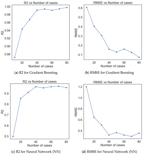
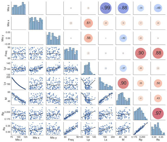
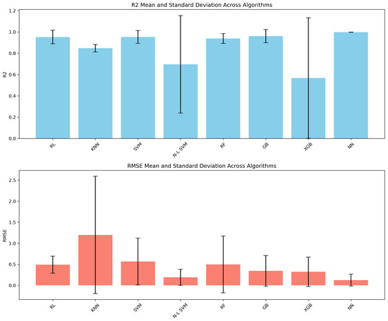
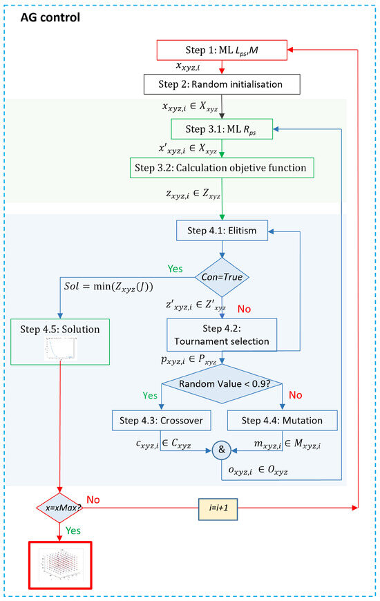
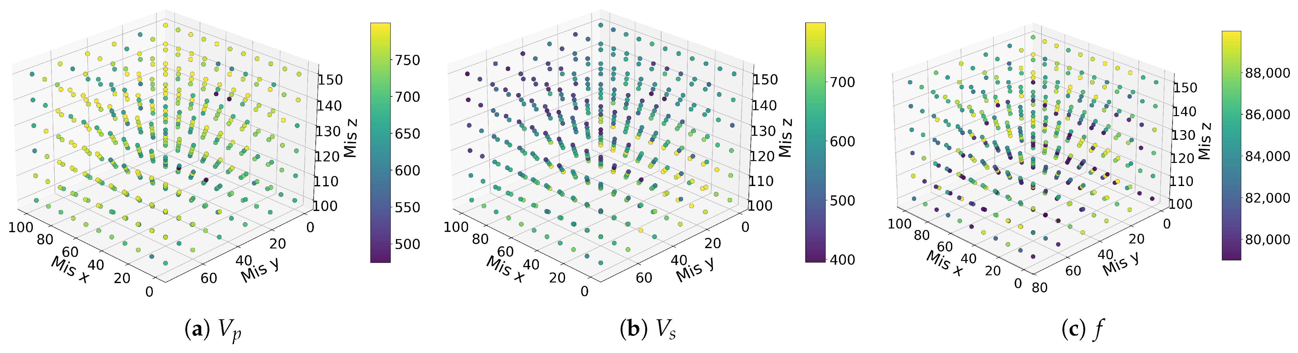
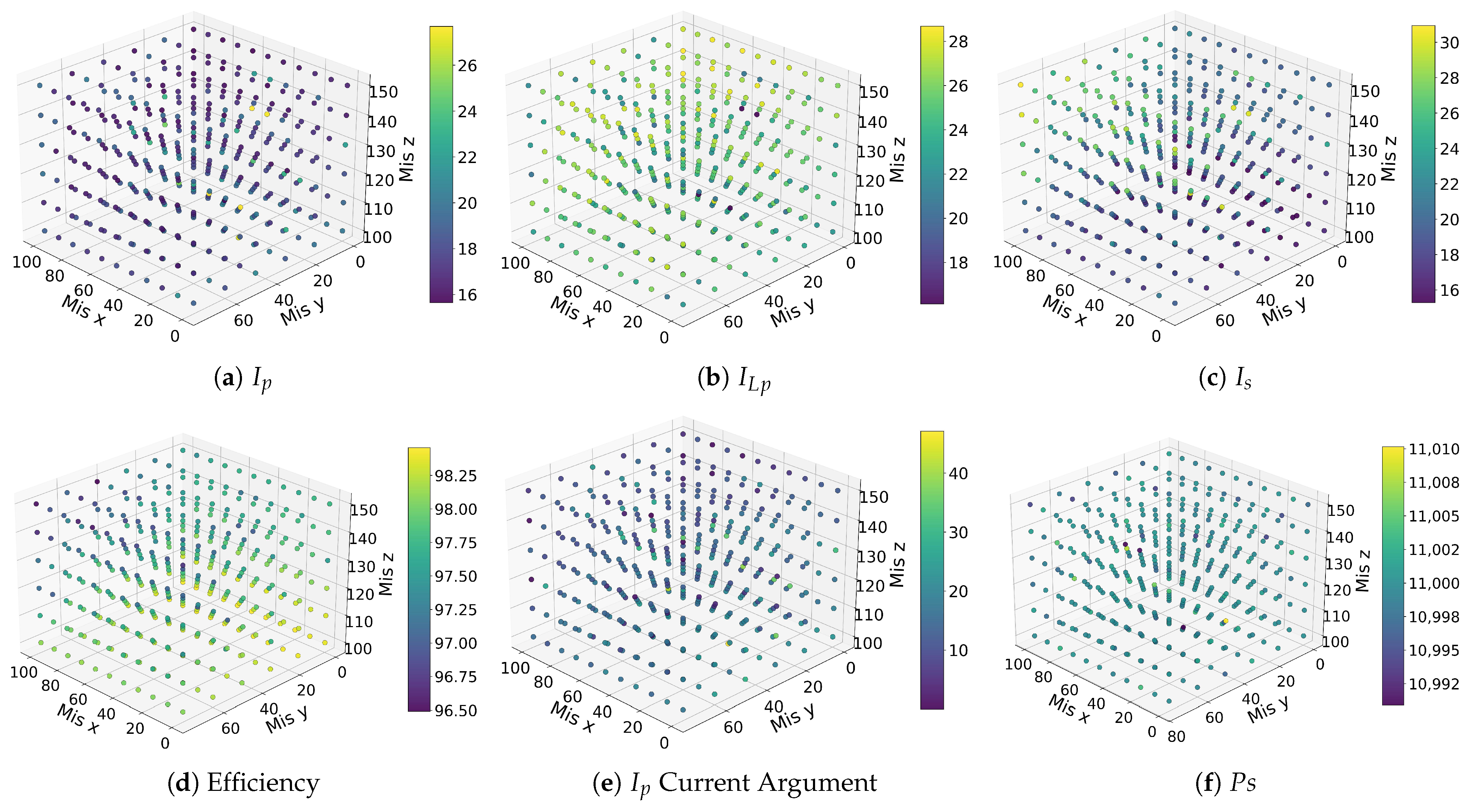
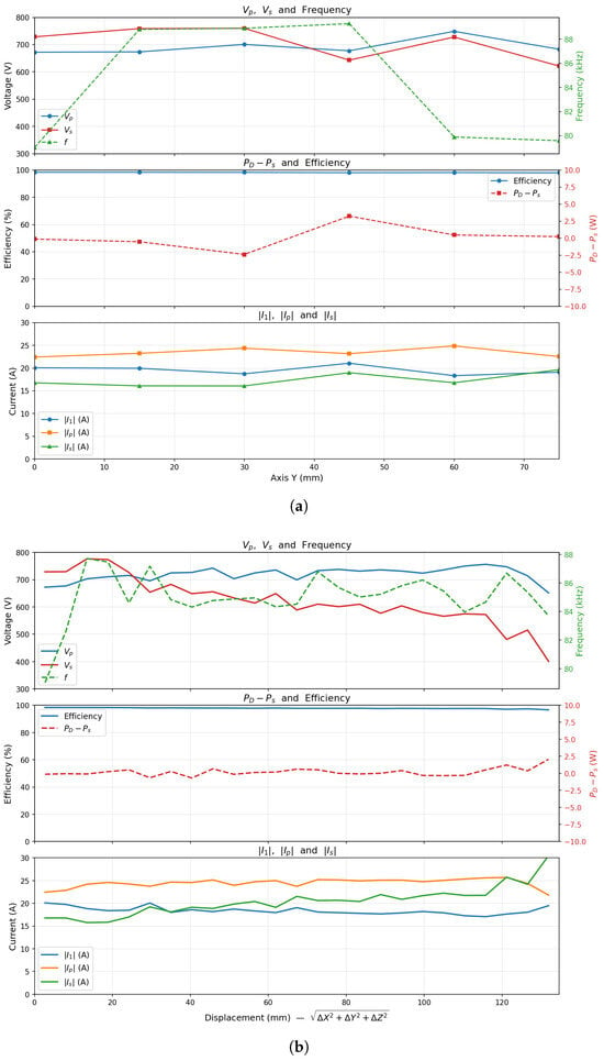
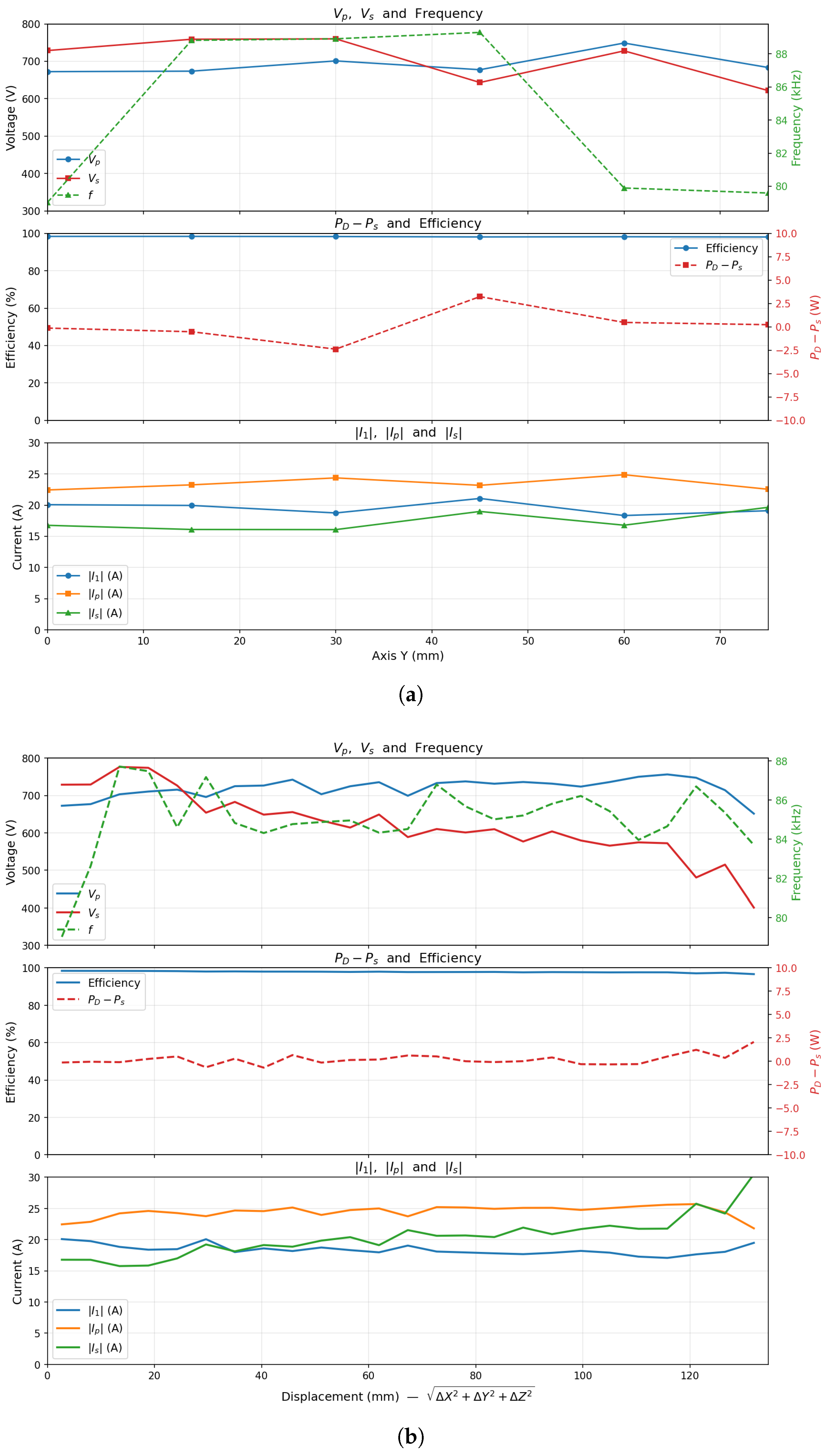
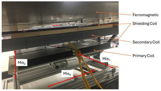
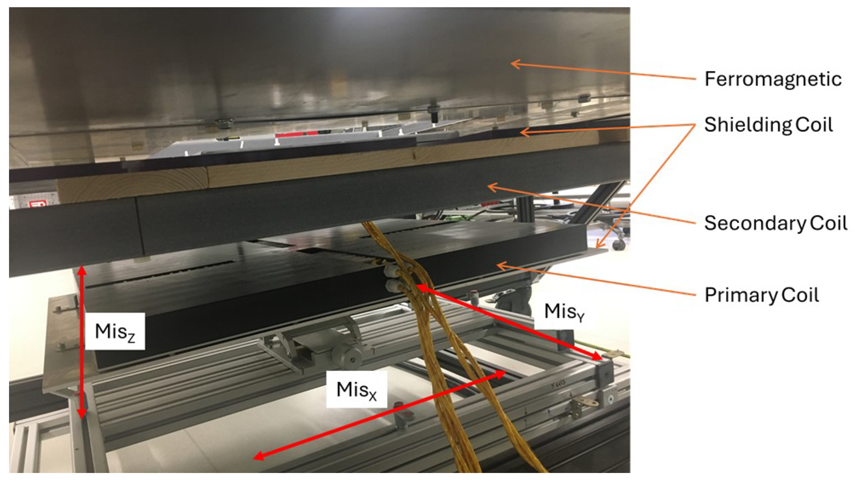
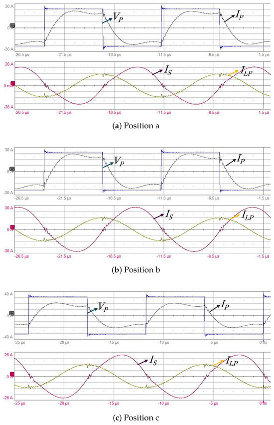
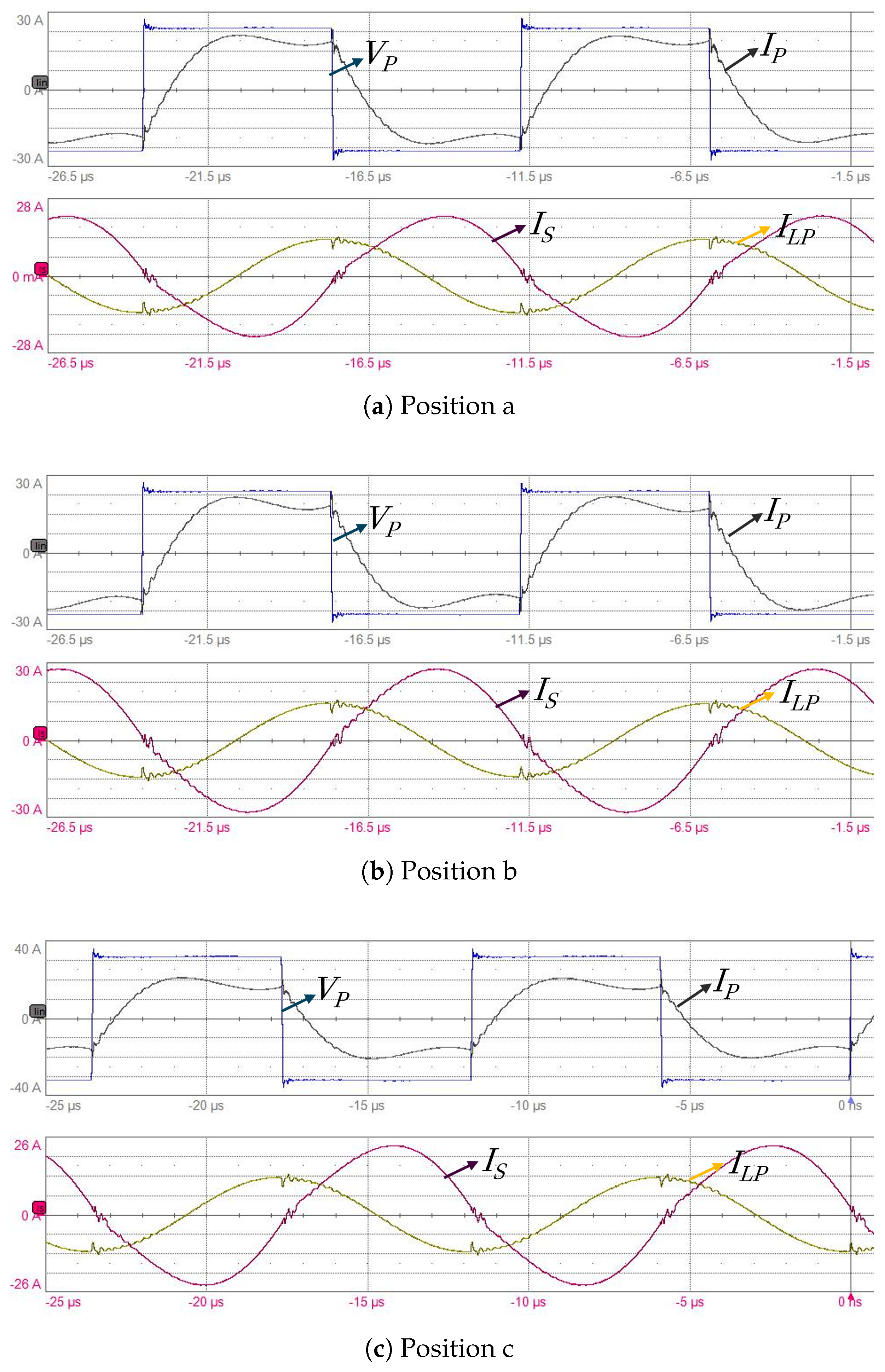
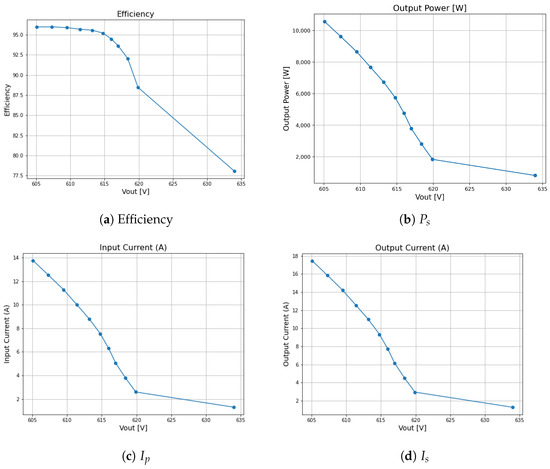
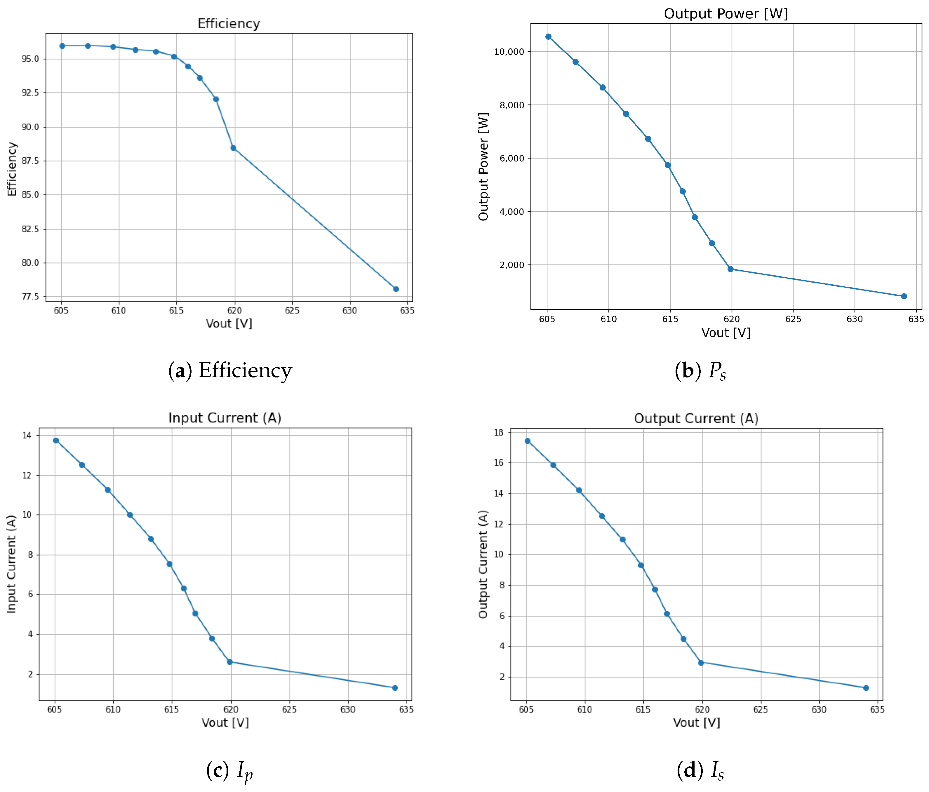

Disclaimer/Publisher’s Note: The statements, opinions and data contained in all publications are solely those of the individual author(s) and contributor(s) and not of MDPI and/or the editor(s). MDPI and/or the editor(s) disclaim responsibility for any injury to people or property resulting from any ideas, methods, instructions or products referred to in the content. |
© 2026 by the authors. Licensee MDPI, Basel, Switzerland. This article is an open access article distributed under the terms and conditions of the Creative Commons Attribution (CC BY) license.