Insights into the Feature-Selection Mechanisms for Modeling the Shear Capacity of Stud Connectors in Concrete: A Machine Learning Approach

Abstract

Shear connections between concrete structural elements play a vital role in defining performance and overall stability. However, limitations in traditional methods for predicting the shear capacity (Vu) of stud connectors in concrete have been highlighted. Developing strategies that precisely describe the performance of stud-headed connectors requires insight into their failure mechanisms and the corresponding shear transmission. Therefore, leveraging advancements in machine learning, this study aims to predict the Vu of the headed stud connector in concrete structures using various input parameters. A database (1121) of the shear strength collected from the literature was trained using six machine learning (ML) algorithms: extreme learning machine (ELM), decision tree (DT), artificial neural network (ANN), multi-linear regression (MLR), support vector machine (SVM), and hybrid ANN–particle swarm optimization (ANN-PSO). Feature selection methods and system identification were applied to explore the optimal or most relevant input parameters. The feature selection techniques indicated that the geometric properties of the stud connector (diameter and cross-sectional area), the concrete modulus of elasticity (Ec), and the height of the weld collar (h_w) are the most relevant input variables. The ANN-PSO model outperformed the other classical models in estimating the shear capacity at two modeling stages. The hybrid ANN-PSO achieved R² = 0.976, MAE = 7.61 kN, RMSE = 10.8 kN, and MAPE = 8.04%, demonstrating the best predictive accuracy among the classical models. On the other hand, DT is the second-best model, with an R² of 0.958, MAE of 10.27 kN, RMSE of 14.43 kN, and MAPE of 8.53 kN for forecasting the shear capacity of stud connectors in concrete.

1. Introduction

Due to their superior production conditions, shorter construction time, weight savings, and lower life-cycle costs, full-depth precast concrete deck structures are increasingly used in bridges and buildings. To enhance structural integrity and decrease superstructure depth, precast concrete deck structures are typically built in composite with supporting girders [1,2,3]. To minimize field-cast connections and streamline production and erection processes, most composite structures employ clustered shear connectors spaced far apart [4]. Shear capacity in stud connectors plays a critical role in determining overall structural performance, such as stiffness and strength [5], and in ensuring monolithic behavior between concrete and steel structures. Their primary function is to resist shear stress at the interfaces of composite structures, such as beams, columns, and slabs, and to prevent vertical separation between the concrete and the structure. Numerous types of shear connectors have been established to form a composite section during construction. The commonly used headed stud stems can be easily installed through composite members [6].

Wu et al. [1] identified two main failure mechanisms of steel–high-strength fiber-reinforced concrete (HSFRC) girder composites formed with welded stud and perforbond rib connectors and tested under a push-out test. The findings demonstrate that while the ductility of the welded stud and one-hole Perfobond rib connectors decreased, the shear capacity and stiffness of the stud connectors rose when used in steel–HSFRC composite girders. Kumar and Chaudhary [7] reported that the shear capacity of studs improves with higher reinforcing bars; subsequently, they offered a restraint effect on the adjoining structural concrete. Shim et al. [8] carried out push-out tests to investigate the performance of stud connectors arranged in groups. The results showed that the stud arrangement is the primary factor in the design criteria for the group stud connector.

Over the past few decades, various empirical equations have been developed to predict the shear capacity of studs in composite structures. For instance, Ollgaard et al. [9] investigated the shear resistance of stud connectors of different sizes (16 and 19 mm diameter) fixed in concrete using a push-out test, and developed a model for shear resistance considering concrete properties. The effect of the maximum tensile strength of the stud was not captured for establishing the design model. A regression model was created to determine the relationship between observed concrete characteristics and failure stress. The authors proposed Equation (1) to predict the average shear resistance of a headed stud connector.

$$P_{Rm}=1.106A_s{f}_{cm}^{0.3}{E}_{cm}^{0.44}$$

(1)

Moreover, Equation (1) was evaluated to assess the impact of rounding down exponents to account for concrete failure, as advised for design when h_sc/d ≥ 4.2. [10]

$$P_{Rm}=0.5A_s\sqrt{f_{cm}{E}_{cm}}$$

(2)

where A_s, h_sc, and d are the dimensional parameters: area, height, and diameter of the stud shank.

The upper bound on the stud strength was determined using Equation (2), which compared the failure load from the push-out tests, such as when $\sqrt{f_{cm}{E}_{cm}}$ ≥ 895 (MPa), which corresponds to the stud material’s ultimate tensile strength.

The American Institute of Steel Construction Specification [11] adopted Equation (2) in 1986 as the design technique for evaluating the shear resistance of headed studs, considering an upper limit demonstrating ‘steel failure’ of the stud itself:

$$P_{Rm}=A_s{f}_u$$

(3)

where f_u is the ultimate tensile strength of the stud connector.

Subsequently, Eurocode EC4 [12] has evaluated 75 push-test specimens [13], resulting in the amendment of the coefficients in Equations (2) and (3), collectively with further guidelines when 3 ≤ h_sc/d ≤ 4 [10].

The aforementioned design standard is based on empirical methods derived from push-test findings. Nevertheless, there is some ambiguity regarding the primary material and dimensional features that influence shear resistance. Therefore, data-driven techniques for stud connectors in composite constructions are being developed using advanced artificial intelligence (AI), focusing on ML models that can learn and perform tasks and solve complex problems. ML algorithms have been used in evaluating engineering structures’ performance, including material properties, structural behavior, and degradation properties [14]. For instance, in the modeling of hot-rolled and cold-formed steel elements [15,16], concrete properties [17,18], masonry structures [19], steel–concrete composites [20,21,22], and fiber-reinforced polymer-strengthened steel or concrete [23,24,25], Wang et al. [26] predicted the bond strength of concrete—steel composites using the ML approach. Wang et al. [27] used an ensemble model for forecasting the shear capacity of stud connectors. The authors applied the LightGBM model hybridized with Gaussian processes (GP) for the modeling task. After the shear mechanisms of studs were examined, feature extraction and combination were used to incorporate them into the models. Razavi et al. [28] used a wide dataset to train six ML models for forecasting the shear capacity of stud connectors. Compared with the other models, the proposed support vector machine (SVM) technique with optimal hyperparameters performed better.

Traditional approaches have demonstrated limitations in estimating shear capacity in concrete structures because they do not account for the full effects of various factors. Leveraging advances in machine learning, the research aims to develop a practical, innovative tool for engineers that enhances the safety and reliability of structures. To meet the need for practical, precise structural evaluations, the study aims to bridge the gap between theoretical models and the challenges they face in practice. Ultimately, the research aims to advance the knowledge base in structural engineering by providing insights into predicting shear resistance using machine learning. The study aims to leverage machine learning (ML) techniques to accurately predict the shear capacity of stud connectors fixed in concrete structures. The application of ML models has extended the optimization capabilities of ANN-PSO, improving prediction accuracy, reducing reliance on classical methods, and enabling the practical use of ML in composite structures. A large database from the experimental push-out tests for stud connectors in concrete was collected from the literature involving mechanical and geometric parameters. System identification was applied to explore the most relevant parameters. Neural networks (NN) for system identification were used to enhance precision, adaptability, and expandability in comparison to conventional techniques, particularly in intricate and non-linear systems.

2. Materials and Methods

2.1. Dataset Development

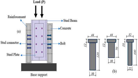
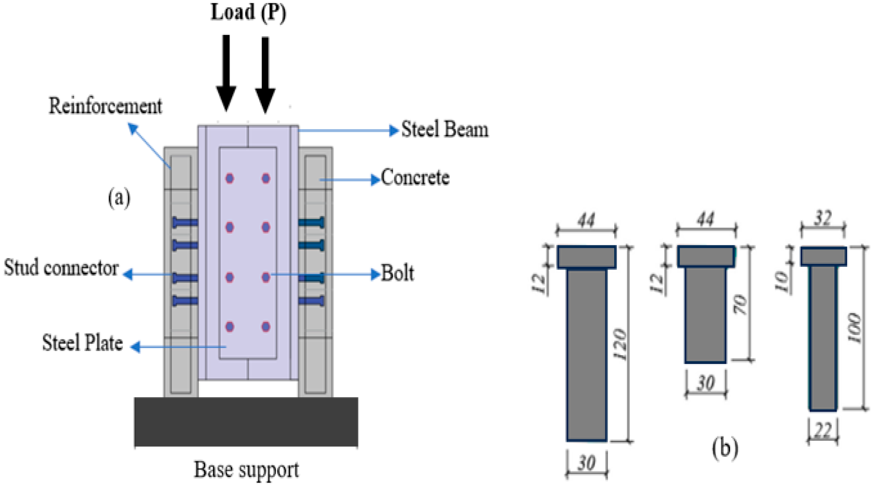
The shear resistance of stud connectors is generally evaluated through a push-out test (Figure 1). Eurocode 4 (EC4) specifies this push-out test [29]. Many input variables are used in developing a shear resistance prediction model. Table 1 summarizes the input variables considered in model development. There are nineteen (19) potential input variables for predicting the shear capacity of stud recorded in the literature. However, some input variables in a dataset may be irrelevant to the model’s predictive performance; therefore, Table 2 summarizes the input variables available in the dataset developed for the study. Twelve (12) input variables are included in the dataset according to the feature selection method. The results of push-out experiments for the stud connections from previous studies were collected in various ways to develop the dataset. The datasets from previous studies [28,30] were merged to form the most extensive dataset, accruing 1121 data points. The collection covers 78 batches of experiments conducted over the past decades. The largest dataset for the stud connector under shear capacity was developed by combining two databases from [28,30], totalling 1121 data points from 78 batches of push-out tests conducted over the past decades.

Figure 1. (a) Systematic illustration of the push-out experimental setup, (b) typical stud connectors.

Table 1. Potential input variables used for shear resistance predictions.

SN	Direction	Variable	Symbol	Units
1		Compressive strength	fcm	MPa
2		Concrete secant modulus of elasticity	Ecm	’’
3		Stud’s tensile strength	fu	’’
4		Yield strength of reinforcement	fy	’’
5		Confining stress of stirrup on concrete	fyρsv	’’
6		Diameter of stud	ds	mm
7		Height of stud	hs	’’
8		Diameter of weld collar	dw	’’
9		Height of weld collar	hw	’’
10		Spacing of stud connectors	st	’’
11		Transverse spacing of stud connectors	st	’’
12		The tensile capacity of stud shank	fsuAs	kN
13	Inputs	Strength and elastic modulus	(Ecmfcm)1/2	kN
14		Area of stud shank	As	mm2
15		Projected area	Aw = dwhw	mm2
16		Aspect ratio	hs/ds	-
17		Effective thickness of concrete	tc/ds	-
18		Stirrup ratio	ρsv	%
19		Stud number per slab	ns	Mm
1	Output	Shear resistance	Vu	kN

Table 2. Input variables used for the study.

SN	Direction	Variable	Symbol	Units
1		Compressive strength	fcm	MPa
2		Concrete secant modulus of elasticity	Ecm	’’
3		Stud’s tensile strength	fu	’’
4		Diameter of stud	ds	mm
5		Height of stud	hs	’’
6	Inputs	Diameter of weld collar	dw	’’
7		Height of weld collar	hw	’’
8		Stud shank’s tensile strength	fsuAs	kN
9		Area of stud shank	As	mm2
10		Strength and modulus of elasticity	(Ecmfcm)1/2	kN
11		Projected area	Aw = dwhw	mm2
12		Aspect ratio	hs/ds	-
1	Output	Shear resistance	Vu	kN

2.2. Dataset Preparations

Data preparation or data preprocessing is an essential stage in developing machine learning models. The quality of the dataset heavily influences the performance and generalization of the shear resistance model. In this study, data preparation, normalization, and feature selection were performed to assess the quality of the dataset.

Dataset Normalization

Data normalization is a preprocessing step in machine learning that rescales and standardizes numerical features in a dataset. The objective is to standardize all features, ensuring that no single feature dominates, particularly for algorithms sensitive to the number of input features. Normalization preserves the structure of data distribution while ensuring that the scales of distinct features are comparable. The Min–Max Scaling technique is the most common normalization method and is adopted in this study, as shown in Equation (4). It scales a feature’s values to the [0, 1] range.

$$x_{norm}={\displaystyle \frac{x_i-x_{\min }}{x_{\max }-x_{\min }}}$$

(4)

where x_norm is the normalized variable, and x_min and x_max are the minimum and maximum values of x_i.

2.3. Machine Learning Algorithms

Numerous researchers have demonstrated that machine learning algorithms have achieved highly satisfactory outcomes in various domains, including physics, mathematics, health, military, engineering, and economics, by emulating the functionality of brain neurons [22,31,32,33,34]. Recently, ML revealed promising results in predicting the performance of construction materials and structural elements. This study used six (6) machine learning algorithms to forecast the Vu of the stud connectors. These algorithms are as follows.

2.3.1. Artificial Neural Network (ANN)

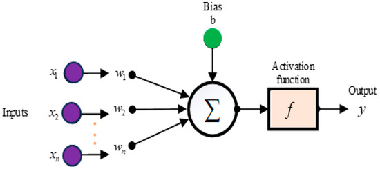
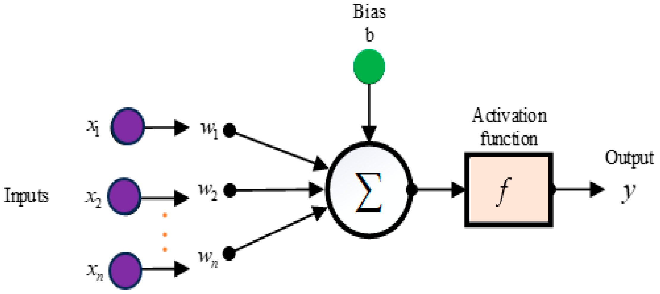
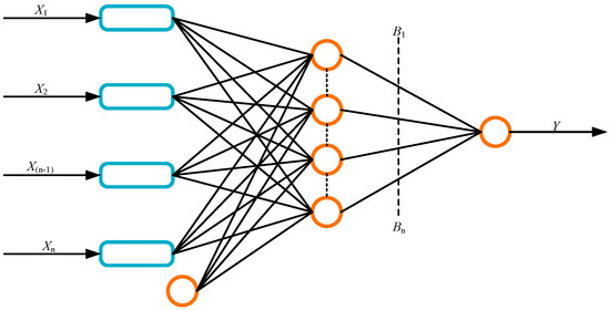
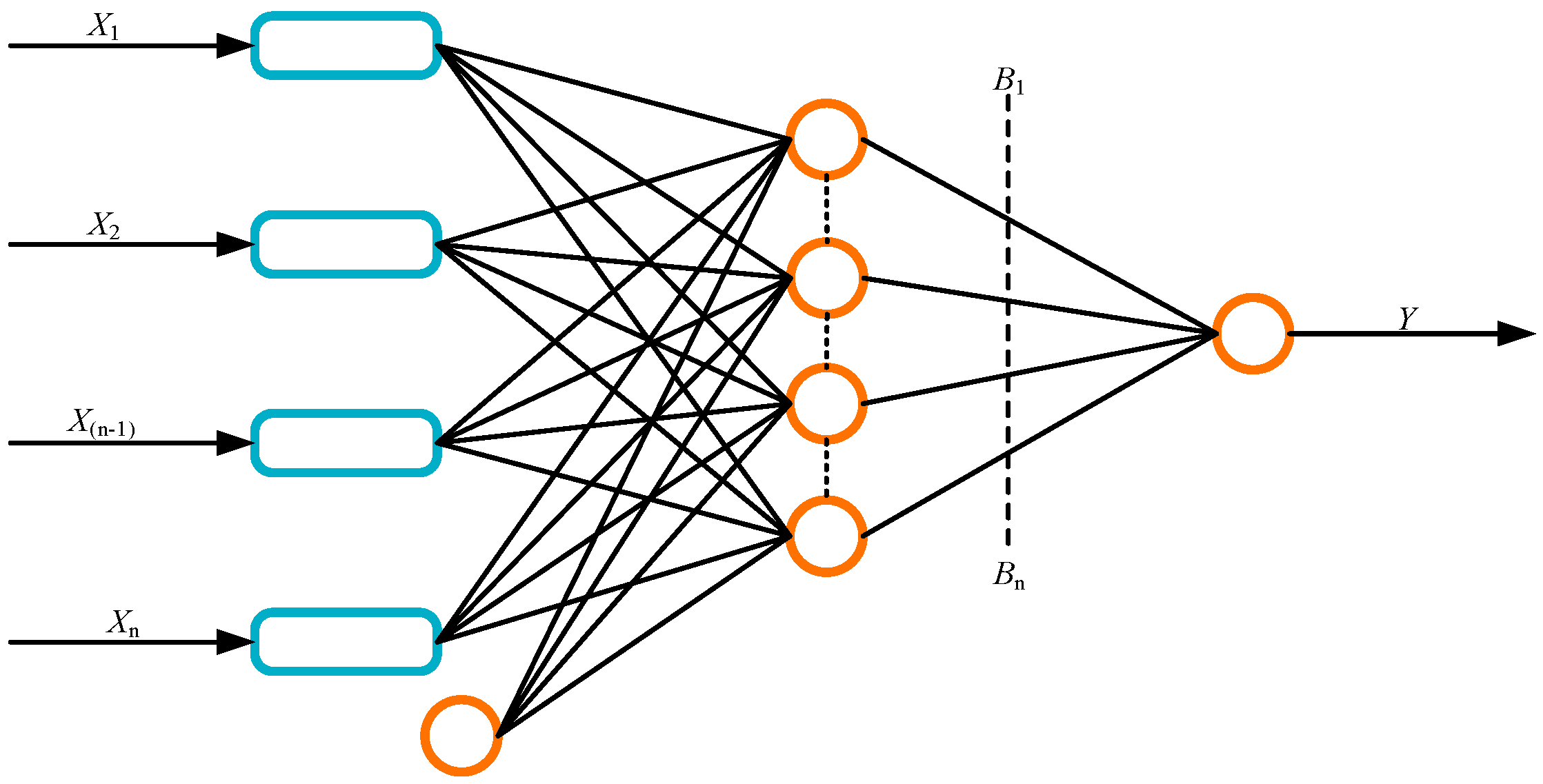
The ANN is widely regarded as the most commonly employed ML algorithm [35]. It has the capacity to acquire new knowledge through learning, information retention, and generalization by emulating human brain function. ANN, which has broad applications, including classification, prediction, optimization, regression, and pattern recognition, comprises three fundamental components. An ANN architecture consists of an input layer that connects to the input variables, an output layer that produces the output features, and a hidden layer between the input and output layers. A typical ANN architecture is presented in Figure 2. The sum of a neuron’s computed weights and biases is referred to as the Net. Its mathematical expression is given in Equation (5) [36,37].

$$\mathrm{Net}={\displaystyle {\sum }_{i=1}^n{w}_{ij}{x}_i+b_i}$$

(5)

Figure 2. ANN architecture.

A hyperbolic tangent function has been employed in the investigation to enhance the output [38]. The function is bounded between −1 and 1, and it is defined in Equation (6).

$$y=f\left(Net\right)={\displaystyle \frac{2}{1+e^{-2.net}}}-1$$

(6)

where x_i is the input variable in the ith hidden layer and y is the target variable, f is the activation function, and w_i and b_i are the biases and weights in the ith hidden layer.

2.3.2. Multiple Linear Regression (MLR)

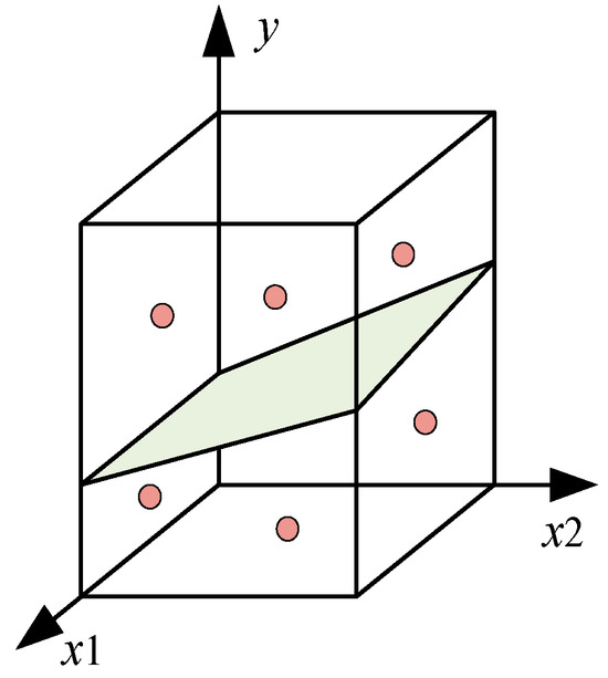
MLR is a commonly used machine learning technique that estimates the linear regression model between a set of independent variables (denoted X, where X ∈ Rn × m) and a dependent variable (denoted y, where y ∈ Rn × 1). The mathematical expression for MLR is given in Equation (7), and the structure of MLR is shown in Figure 3.

$$y={\omega }_0{x}_0+{\omega }_1{x}_1+\dots {\omega }_n{x}_n={\displaystyle \sum _{i=1}^n{\omega }_i{x}_i}={\omega }^{T}x$$

(7)

Figure 3. MLR structure.

The variables ω₁… ω_n represent the partial regression coefficients of the technique. The variable ω₀ corresponds to the intercept on the y-axis when x₀ is equal to 1.

2.3.3. Decision Tree (DT)

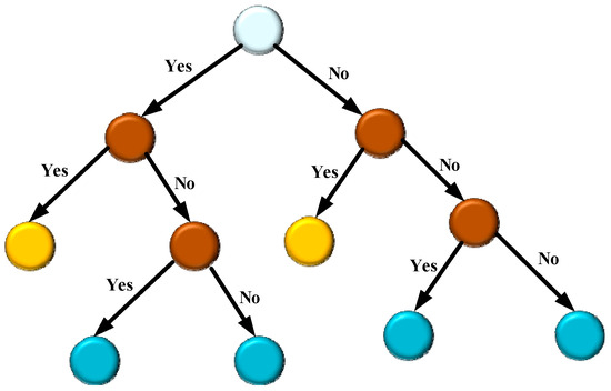
A popular supervised ML method for regression and classification issues is the decision tree. Using training data, it develops a model of a tree-like structure [39]. The root node of the tree-structured algorithm branches into nodes corresponding to the test outcomes for each feature. The DT technique tends to overfit the data when compared to other models due to the considerable variety of a single decision-tree model [40]. To create a decision tree, two stages are required: partitioning the feature space of the training dataset into H mutually exclusive and exhaustive subsets. The measure of total variation across all j classes is described by the Gini index (GI), which is utilized for the binary separation procedure for sections [41]. The DT structure is shown in Figure 4.

$$GI=\sum _{J=1}^3\widehat{P}nj(1-\widehat{P}nj)$$

(8)

where $\widehat{P}nj$ represents the training set assembly in the nth region for the jth class. Cost-complexity pruning, which uses a collection of trees indexed by the non-negative tuning parameter α, can be used to prevent overfitting and overly complex trees. The k-fold validation approach may be employed at this step to obtain the maximum α-value, since the GI of the holdout data has decreased.

Figure 4. A typical DT structure.

2.3.4. Support Vector Machine

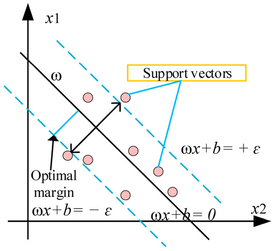
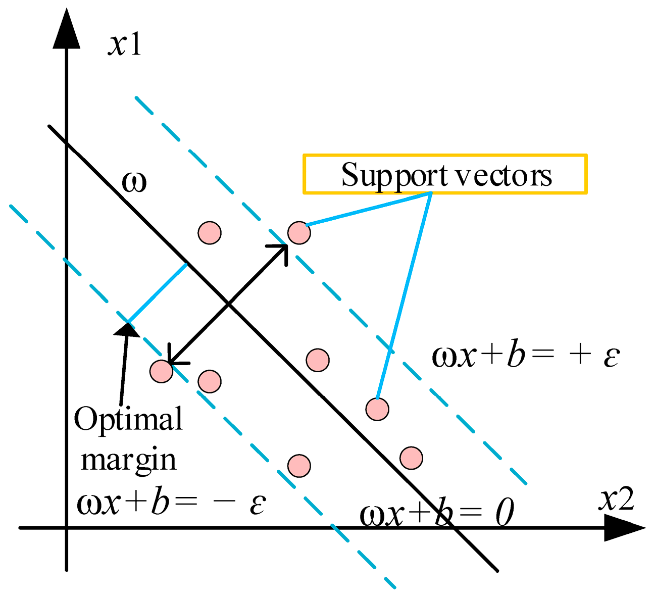
The SVM algorithm is a powerful, state-of-the-art supervised machine learning method commonly used for regression and classification tasks. In bridge engineering, the technique has shown promising results, as well as in many civil engineering fields [42]. This model was first developed by Vapnik et al. [43]. It uses the input variables to map the primary input space into a higher-dimensional feature space via a nonlinear mapping. The typical representation of a support vector machine is presented in Figure 5.

Figure 5. Structure of SVM.

Given a dataset consisting of a collection of training points {(x₁, t₁), …, (x_n, t_n)}, where x₁ is an input variable in the n-dimensional space Rⁿ, and t_i is an output variable in the one-dimensional space R¹. The linear SVM function f(x) transforms the input vector x_i into the output vector t_i using a mapping process.

$$f\left(x\right)={\omega }^T\varphi \left(x\right)+b$$

(9)

The variables ω and b represent the support vector and bias, respectively. The discrepancy between the target value f(x) and the goal output t is referred to as an ɛ-insensitive loss function (L_ɛ) and is mathematically represented in Equation (10).

$$L_{\epsilon }(t)={\left|\left.t-f(x)\right|\right.}_{\epsilon }=\left\{\begin{array}{c}0\hspace{1em}\hspace{1em}\hspace{1em} \mathrm{if} \left|\left.t-f(x)\right|\right. \le \epsilon \\ {\left|\left.t-f(x)\right|\right.}_{\epsilon }, \mathrm{otherwise}\hfill \end{array}\right.$$

(10)

The deviation of f(x) from the actual output t_i is limited to an ɛ-precision level and can be accomplished by minimizing ω^Tω, as in Equation (11):

$$\begin{array}{l}\min {\displaystyle \frac{1}{2}}{\omega }^T\omega \\ subjected \mathrm{to} \left\{\begin{array}{l}{\omega }^T\varphi \left(x_i\right)+b-t_i\le \epsilon ,\\ t_i-{\omega }^T\varphi \left(x_i\right)-b\le \epsilon , \end{array}\right.\end{array}$$

(11)

2.3.5. Extreme Learning Machine

The concept of ELM was initially developed by Huang et al. [44]. Recently, it has become a widely used tool for making predictions [45]. The model assumes that every continuous function in the input space can be accurately approximated by the random input’s weights and biases [45]. The methods can be used to compute a single-layer feedforward neural network (SLFN) without iterative processing. Therefore, the ELM provides a rapid approach for training the single-layer feedforward network (SLFN) and reliably identifying all network parameters, while preventing any undesired human intervention [46]. The ELM procedure consists of three steps: (1) building the SLFN; (2) assigning the SLFN weights and biases at random; and (3) using the hidden layer output matrix to calculate output weights [47]. The ELM architecture is depicted in Figure 6.

Figure 6. An ELM architecture.

2.3.6. Particle Swarm-Optimized ANN (PSO-ANN)

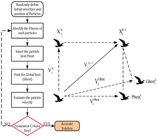
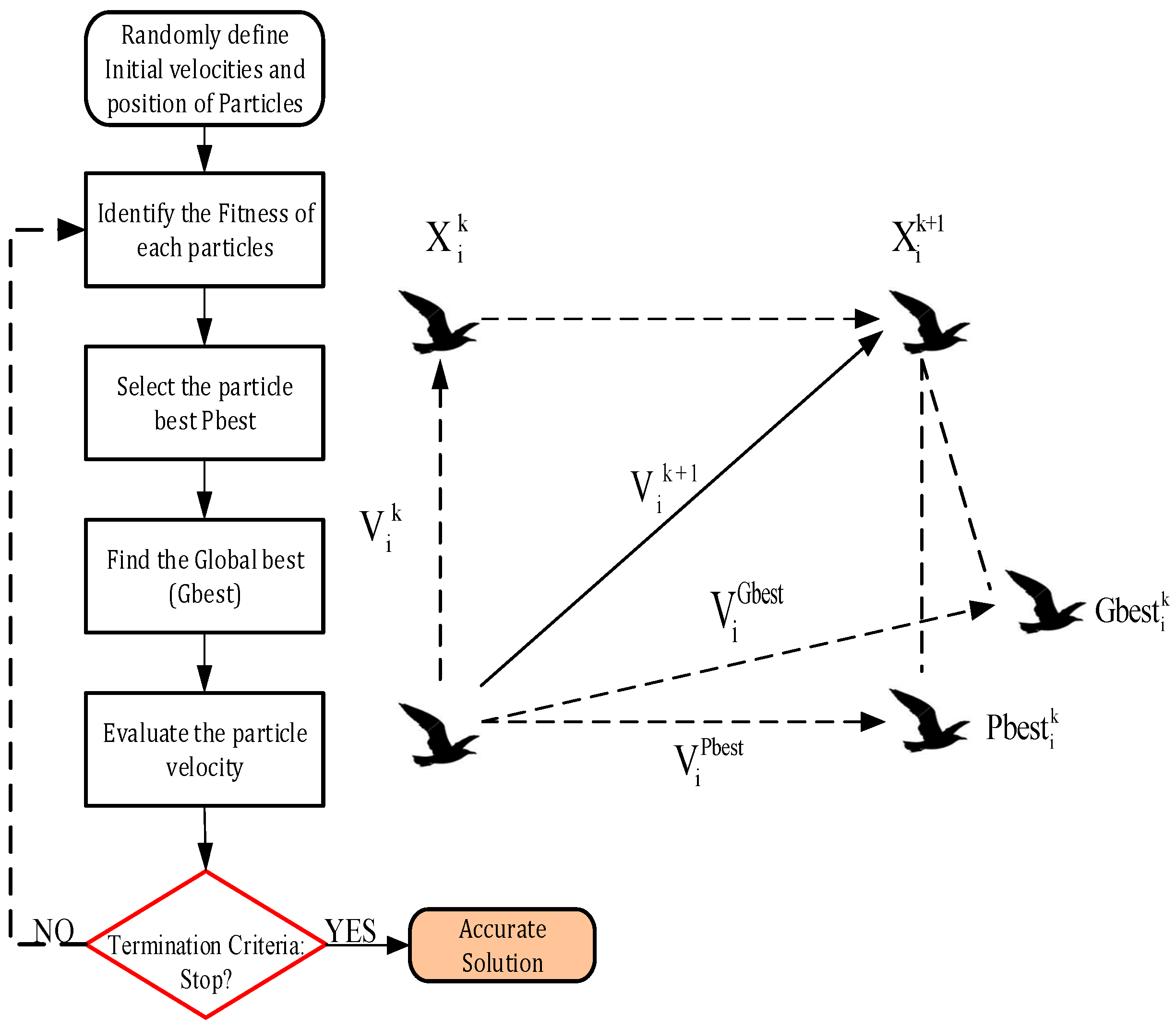
The PSO is a metaheuristic method developed by Eberhart and Kennedy [48] that uses evolutionary computation to simulate the collective behavior of bird flocks. PSO has demonstrated efficacy in numerous complex problems [49]. The bird represents the element, and its group comprises possible outcomes within the exploration area. Every particle is generated randomly within the region and moves with a specific velocity, as depicted in $\begin{array}{l}\\ V_{\min }\le V_{i,j}^k\le V_{\max }\end{array}$ Figure 7. Each cycle ends with the storage and evaluation of the personal best (Pbest) and global best (Gbest) particles. The most recent generation is obtained by updating each particle’s velocity and position according to Equations (12) and (13).

$$\begin{array}{l}{V}_{i,j}^{k+1}=w{V}_{i,j}^k+c_1{r}_1\left(P_{\mathrm{best} i,j}^k-X_{i,j}^k\right)+c_2{r}_2\left(G_{\mathrm{best} i,j}^k-X_{i,j}^k\right) \\ V_{\min }\le V_{i,j}^k\le V_{\max }\end{array}$$

(12)

$$X_{i,j}^{k+1}=X_{i,j}^k+V_{i,j}^{k+1}$$

(13)

Figure 7. PSO flow chart.

The variable P^k_{best i,j} denotes the personal best value of the jth component for the ith individual. G^k_{best i,j} represents the value of the jth element for the global best location at iteration k. V^k_i,j indicates the velocity of the particle (i,j) at the kth iteration. X^k_i,j denotes the location of the particle at iteration k, with j and I denoting its coordinates.

2.4. Model Development, and Performance Evaluation

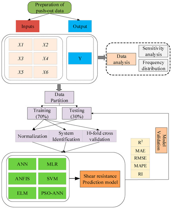
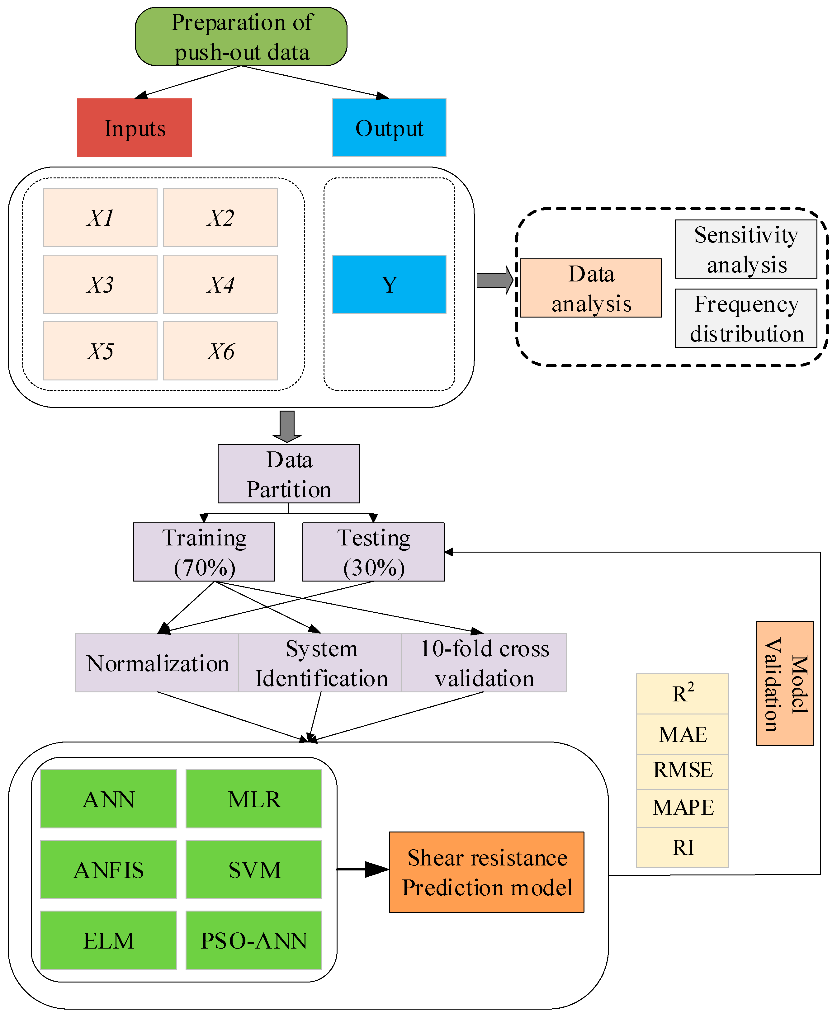
The study aims to develop machine learning models to forecast shear capacity accurately. Figure 8 presents the schematic representation of the model developments. The input variables and the output variable were first analyzed using system identification and frequency distribution analysis. The data was then partitioned into 70/30 for training and testing. Several ML algorithms were used to develop shear resistance models. Four evaluation matrices were utilized to determine model performance, as given in Equations (14)–(17). The R² value indicates the proportion of variance in the observed data that is explained by the model. MAE and RMSD are used to assess the prediction error. The prediction error is nearly zero, resulting in improved predictions.

$$R^2={\left[{\displaystyle \frac{{\displaystyle {\sum }_{i=1}^n(y_i-\overline{y})(p_i-\overline{p})}}{\sqrt{{\displaystyle {\sum }_{i=1}^n{(y_i-\overline{y})}^2{\displaystyle {\sum }_{i=1}^n{(p_i-\overline{p})}^2}}}}}\right]}^2$$

(14)

$$\mathrm{MAE}={\displaystyle \frac{1}{n}}{\displaystyle {\sum }_{i=1}^n\left|y_i^{\prime }\right.}-\left.y_i\right|$$

(15)

$$\mathrm{RMSE}=\sqrt{{\displaystyle \frac{{\displaystyle {\sum }_{i=1}^n{(y_i^{\prime }-y_i)}^2}}{n}}}$$

(16)

$$MAPE={\displaystyle \frac{1}{n}}{\displaystyle {\sum }_{i=1}^n\left|\left.\frac{y_i^{\prime }-y_i}{y_i}\right|\right.}\times 100$$

(17)

where n = sample number, y_i^’ is the observed value, and y_i is the target feature. Furthermore, the computer system and software environment are used to develop the code and assess the model’s performance. The computer system used for this inquiry was an Intel(R) Core(TM) i5-4210H CPU I@ 2.90 GHz with 8.0 GB of RAM, and the code was developed in MATLAB version 2023a.

Figure 8. Flow chart of the model development.

3. Results

3.1. Hyperparameter Tuning

To enhance the overall accuracy and stability of the various models, hyperparameter tuning was conducted. For the ANN, the focus was on the hidden neurons, activation functions, and learning rate, while for the MLR, the strength of the regularization was adjusted. For the decision tree, the significant performance indices were the maximum depth and the pruning coefficient. In contrast, the SVM required tuning of the regularization constant, the epsilon margin, and the kernel parameters. For the ELM, the number of hidden neurons and the regularization term were selected to balance speed and accuracy. The ANN-PSO hybrid model required tuning both the ANN architecture and the PSO search strategy, enabling adaptive, optimal distributed search. Overall, the results from models with tuned hyperparameters were favorable, and model generalization improved, with the ANN–PSO model achieving the best performance. Table 3 summarizes the hyperparameters used in this study.

Table 3. Hyperparameters.

Model	Hyperparameter	Value
ANN	Number of hidden neurons	100
	Activation function	tanh
	Learning rate	0.005
	Epochs	2000
	Batch size	32
MLR	Fit intercept	True
	L2 regularization (α)	0.1
Decision Tree	Maximum depth	20
	Minimum sample split	5
	Minimum sample leaf	2
	Pruning parameter (α)	0.01
SVM	C (regularization constant)	100
	ε (epsilon loss)	0.05
	Kernel	RBF
	Gamma	0.01
	Hidden neurons	500
	Activation function	sigmoid
	Regularization (λ)	0.1
ANN–PSO	ANN hidden neurons	80
	PSO population size	50
	PSO iterations	200
	Inertia weight (ω)	0.7
	Cognitive coefficient (c1)	2.0
	Social coefficient (c2)	2.0
	Velocity limit	±50

3.2. Data Distribution

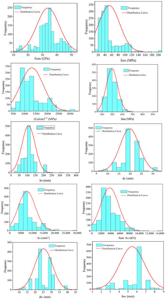
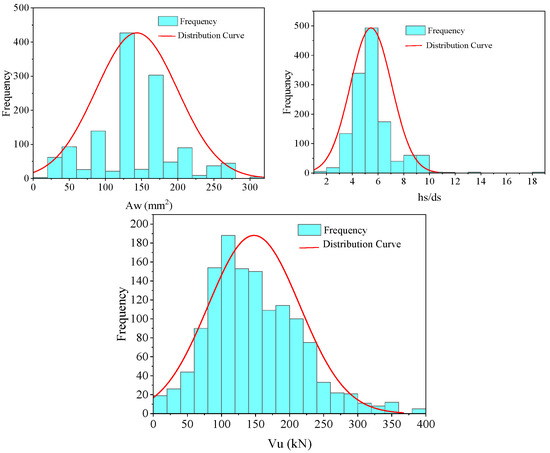
The comprehensive datasets obtained were analyzed using data distribution to characterize the data. The distribution of each of the twelve (12) input variables in the data set is shown in Figure 9. Figure 9 shows that some parameters, such as the concrete secant modulus of elasticity, the stud tensile strength (fu), and the dimensional features (hs, ds, dw, and Aw), are normally distributed, with their means at the midpoint of the superimposed distribution curves. However, input features, such as concrete compressive strength (fcm), projected area of the welded collar, and height of the welded collar, do not follow a normal distribution. The statistical parameters for the selected input-feature modeling task are summarized in Table 4.

Figure 9. The distribution plots of the individual feature in the database.

Table 4. Statistical indicator of the dataset.

Direction	Symbol	Maximum	Minimum	Mean	Std.	Skewness	Kurtosis
	fcm	200	14	53	31.64	1.853	4.089
	Ecm	53,467	10,411	33,896	7776	−0.405	0.577
	fu	900	372	497	56.26	1.278	7.079
	ds	32	5	20	4.252	−0.322	1.071
	hs	400	20	108	40.35	1.749	7.403
Inputs	dw	45	8	25	5.425	−0.007	0.455
	hw	9	2	6	1.279	−1.010	0.727
	fsuAs	14,743	197	391	1907.1	1.238	3.071
	As	28,406	408	743	3812	1.223	2.581
	(Ecmfcm)1/2	3212	495	115	500	1.111	0.808
	Aw	315	16	15	55.15	0.014	0.122
	hs/ds	18	1	5	1.612	1.982	9.631
Output	Vu	397	10	148	67.27	0.634	0.492

3.3. Selection of Optimum Input Parameters

The careful selection of relevant input variables is crucial for achieving the intended, precise output in any data-driven model. Introducing irrelevant factors into the models reduces model accuracy and increases computational requirements, including cost and time [50]. The chosen approach can be achieved using a feature selection method that identifies pertinent features (input parameters) while excluding unnecessary ones, yielding a subset of characteristics that effectively represent the specific problem with minimal performance impact. This study employed two feature selection methods: Pearson correlation (PC) and mutual information.

3.3.1. Pearson Correlation (PC)

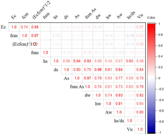
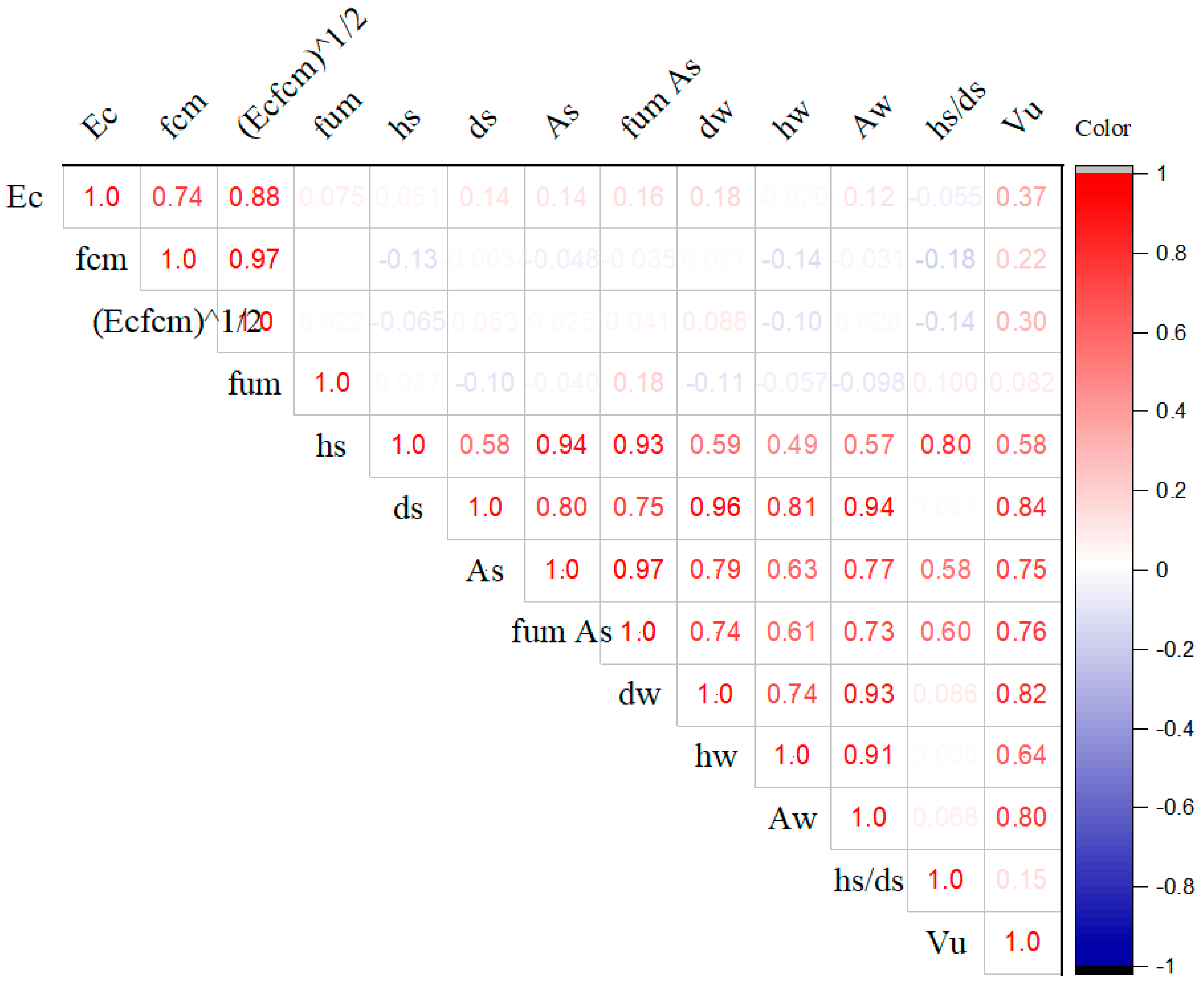
Sensitivity analysis, employed in several studies [51], is a crucial tool for identifying unnecessary input parameters in both linear and nonlinear models. The PC matrix illustrates the influence of each input feature on the prediction of shear resistance (Vu) by presenting the correlation coefficients among the input features, as shown in Figure 10. The variables become less significant as they approach zero and more significant as they approach unity (either −ve or +ve). A parameter that is perfect in every respect is indicated by a unit value of +1 or −1. A positive value indicates that the input and output variables are directly related to stud-connector shear resistance, whereas a negative value indicates an inverse relationship. The PC analysis revealed that dimensional features, such as stud diameter (ds), have the highest correlation coefficient (0.84), followed by the stud cross-sectional area (As) and the weld collar diameter (dw), with PC values of 0.82 and 0.80, respectively. On the other hand, the average tensile strength of the stud connector exhibits the lowest correlation (0.082), followed by concrete compressive strength (fcm), which shows a correlation coefficient (0.22). Lastly, the stud aspect ratio (hs/ds) had a correlation coefficient of 0.15, indicating the lowest relevance in predicting shear capacity.

Figure 10. Pearson correlation matrix.

3.3.2. Mutual Information (MI)

The MI technique is a method for assessing the dependence between input features and the target variable. The MI value ranges from 0 to ∞. An MI value = 0 implies the absence of any statistical dependence between the two parameters. The dependency shows a positive correlation with values that increase from zero [51]. MI is mathematically expressed in Equation (18):

$$MI(r,n)=H(r)+(H(n)-H(r,n))$$

(18)

The joint entropy among the two features, r and n, denoted as H (r, n), is calculated using the entropy function H(r), as expressed in Equation (19):

$$H(r,n)=-{\displaystyle \sum r\in R{\displaystyle \sum n\in N{p}_{RN}}}(r,n)\log p_{RN}(r,n)$$

(19)

The notation p_RN (r, n) represents the joint allocation of the features m and n.

An input feature is considered highly relevant when its mutual information is positive. An MI value of 0 signifies that the possible input features and the failure pattern are completely unrelated [51].

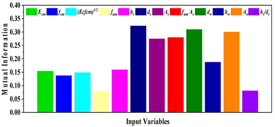
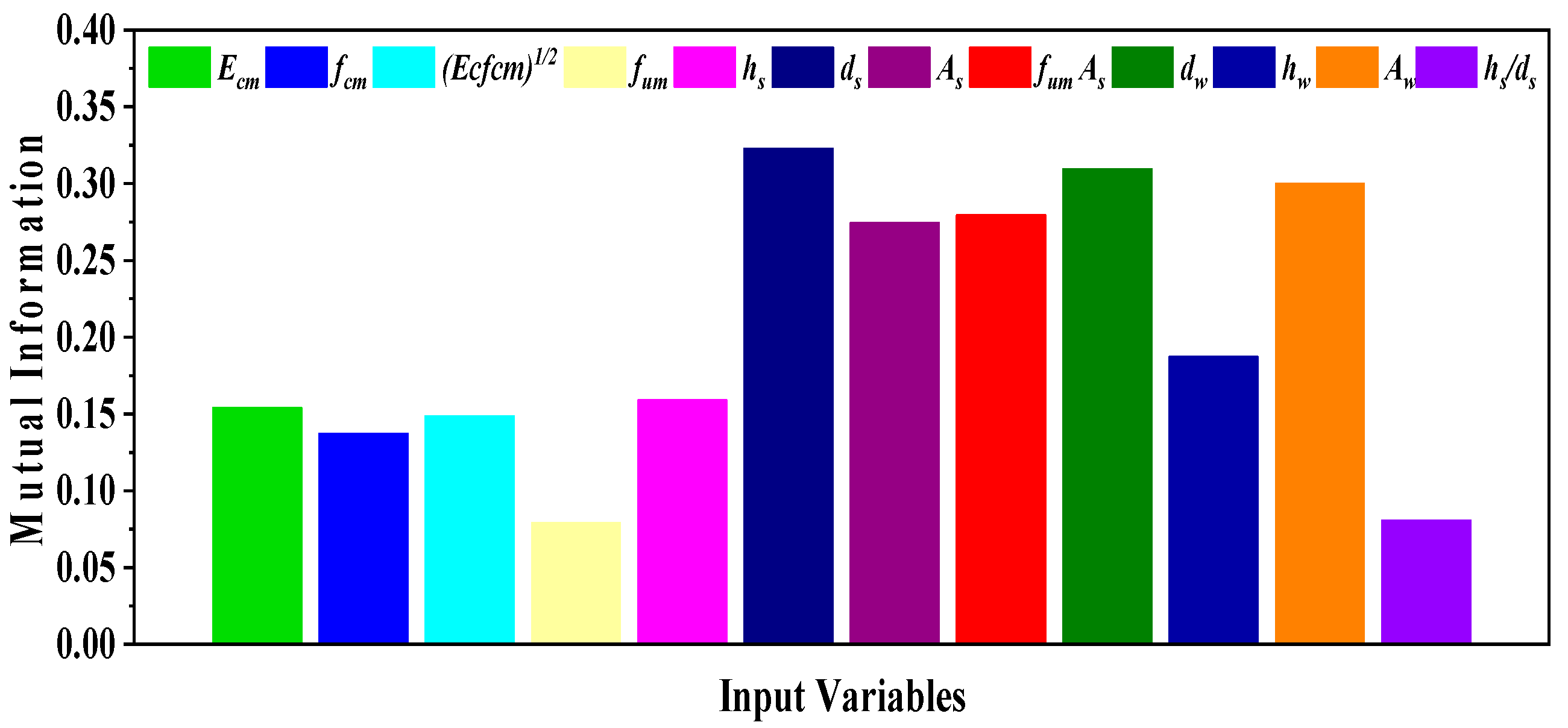
Figure 11 depicts the relevance of each input feature using the MI approach. The dimensional features (d_s, d_w, and A_s) are the most relevant variables with the MI values of 0.322, 0.309, and 0.299, respectively. The least pertinent variables are fum and hs/ds, with MI values of 0.079 and 0.080, respectively, followed by f_cm, with a value of 0.0136. Similar trends were observed using the Pearson correlation matrix. The linear and nonlinear relationships between the input variables and the output variable indicate that the dimensional features are the most relevant, while the mean tensile strength, the aspect ratio of studs, and the concrete compressive strength are the least relevant. Wu et al. [1] identified concrete failure, shank failure, and weld-collar failure of the stud as the primary failure mechanisms of headed studs in concrete. However, these failure patterns are influenced by the concrete strength and the shapes of many elements. Feature selection techniques indicated that concrete strength was less relevant to predicting the shear strength of the stud connector. Although categorical characteristics such as concrete type and interface condition significantly affect stud shear resistance, current equations do not adequately account for these contributions [27]. Concrete compressive strength and elastic modulus alone cannot sufficiently capture differences in material properties across concretes; however, this limitation can be mitigated by classifying concrete types. The potential to fully account for the effects of these elements is enabled by combining features with machine learning models. Various concrete types are included in the database, including normal concrete (NC), high-performance concrete (HSC), engineered cementitious composites (ECCs), ultra-high-performance concrete (UHPC), etc. The AI models must include factors that exhibit both linear and nonlinear interactions with the output features to capture the data’s linearity and nonlinearity accurately.

Figure 11. Mutual information of the input variables.

Therefore, this study employs a system identification technique to describe the relationship between the combined input variables and the target shear resistance. In contrast, the analysis presented captures the relationship between individual variables and the target shear resistance but cannot account for the relationship between combinations of two or more input variables.

3.3.3. The Most Relevant Input Parameters

The feature selection method’s results from the Pearson correlation (PC) and mutual information analysis for selecting pertinent features (input parameters) showed that the dimensional features (ds, dw, As, and hw) and concrete secant modulus of elasticity E_cm are the most relevant variables in predicting the shear capacity of the headed stud connector. These features also relate to shear transfer mechanisms, failure modes, and stress development in the composite sections, reflecting failure in the concrete, stud shank, and weld collar, which are influenced by concrete strength and the shapes of several components. It is essential to investigate the behavior of stud-headed connectors, the shear transmission mechanism, and to develop a technique that precisely describes their performance [52].

The influence of these dimensional features (ds, dw, As, and hw) and concrete secant modulus of elasticity Ecm on the shear capacity of the headed stud connector was an agreed experimental finding from the previous studies [1,53], indicating that an increase in the stud diameter could significantly improve the shear strength, shear stiffness, and ductility of the stud connector. This is attributed to the fact that stud connectors with larger diameters have larger shear areas. Moreover, Wu et al. [1] reported that increasing the stud height had slightly affected the shear capacity of the studs, but it apparently reduced the ductility of the welded studs. For instance, increasing the stud height from 80 to 120 mm increases shear capacity by an average of 1.95%. Confinement also influences the shear capacity of the stud connector; the shear capacity and stiffness of the welded stud are improved in high-performance concrete (HPC) reinforced with steel fibers. Similarly, the shear capacity and deformability of the Perfobond rib connectors increased with increasing perforating rebar diameter. Upon reviewing prior studies, we confirmed that the variables identified by feature selection techniques (PC and MI) are highly relevant for predicting the shear capacity of stud connectors.

3.3.4. Collinearity Assessment of the Most Relevant Features

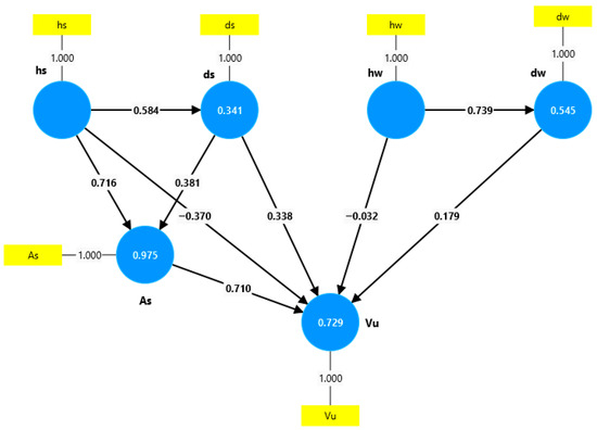
Structural equation modeling (SEM) was employed to assess multicollinearity among the most relevant variables (geometric features, i.e., ds, dw, As, and hw) for predicting the shear capacity of the headed stud connector. The significance of the model is depicted in Figure 12, with collinearity statistics (VIF) for the outer model equal to 1.00 for all variables.

Figure 12. Measurement model (outer loadings and path coefficients).

The Variance Inflation Factor (VIF) analysis indicates no significant multicollinearity among the variables, except for the height of the welded collar (h_w), which has a VIF of 3.246, below the critical threshold of 5.0 [54]. Considering standard thresholds,

• VIF < 5: No multicollinearity concern (ideal);
• VIF 5–10: Moderate multicollinearity (acceptable but monitor);
• VIF > 10: Severe multicollinearity (problematic, requires action).

3.4. Model Detailed Analysis

• Predicting As:

• Vu → As: VIF = 42.994 Severe multicollinearity.

Interpretation: When Vu is used to predict As, there is extreme multicollinearity. This suggests Vu is highly correlated with other predictors in the model. Vu and As may have a strong mathematical or physical relationship.

• Predicting Vu: Vu appears to be an exogenous variable in this model.
• Predicting ds:

• As → ds: VIF = 1.517 ✓ No concern.
• Vu → ds: VIF = 25.463 Severe multicollinearity.

Interpretation: As, when predicting ds, shows excellent collinearity statistics (VIF < 5); however, Vu shows severe multicollinearity when predicting ds. This suggests Vu is highly correlated with other variables in the model, possibly with As or other unmeasured variables. The relationship Vu → ds may be confounded by shared variance with other predictors.

• Predicting dw

As → dw: VIF = 13.771. Severe multicollinearity.

Interpretation: Severe multicollinearity is evident in the prediction of dw, suggesting that As shares substantial variance with other predictors. This high VIF (>10) indicates the standard errors for this path coefficient will be inflated, reducing statistical power and reliability.

• Predicting hs

• As → hs: VIF = 1.517 (no concern)
• Vu → hs: VIF = 23.626 (Severe multicollinearity)
• ds → hs: VIF = 1.000 (Perfect—no collinearity)

Interpretation: As and ds show excellent collinearity statistics. ds has VIF = 1.000, indicating that it is completely independent of other predictors (an ideal situation). Vu again shows severe multicollinearity, a consistent pattern across equations. The pattern suggests Vu is the problematic variable causing multicollinearity issues.

• Predicting hw

• Vu → hw: VIF = 3.246 (acceptable);
• Hs → hw: VIF = 1.000 (perfect—no collinearity).

Interpretation: Both predictors show acceptable VIF values. This is the only equation in which Vu does not exhibit severe multicollinearity. hs shows perfect independence (VIF = 1.000). This equation has the best collinearity profile of all equations.

3.4.1. Overall Patterns and Concerns

I.

Vu is consistently problematic: VIF = 42.994 (predicting As), VIF = 25.463 (predicting ds), and VIF = 23.626 (predicting hs), which is only acceptable when predicting hw (VIF = 3.246).

Implication: Vu appears to be highly correlated with other model variables, causing severe multicollinearity. This indicates Vu shares substantial conceptual overlap with As or other constructs, maybe measurement redundancy, and structural paths involving Vu will have inflated standard errors and unreliable estimates.

II.

The mixed performance is as shown below:

• Acceptable VIF (1.517) when predicting ds and hs;
• Severe multicollinearity (VIF = 13.771) when predicting dw.

Implication: The multicollinearity of As depends on the specific structural equation, suggesting complex interrelationships in the model.

III.

ds and hs show excellent independence:

• Both consistently show VIF = 1.000 or nearly 1.0;
• These variables appear to be well-defined and orthogonal to other predictors.

3.4.2. Collinearity Statistics (VIF) and Statistical Implications

Hair et al. [55] specified PLS-SEM assessments for R² values as the following: R² ≥ 0.75: Strong, R² = 0.50–0.75: Moderate, R² = 0.25–0.50: Weak, R² < 0.25: Unacceptable for key constructs. As shown in Table 5, statistical analysis indicates that As achieved the highest R² of 0.975. The model provides an excellent fit for predicting As, followed by Vu, achieving R² = 0.729. In total, 72.9% of the indicated variance in Vu is explained by its predictors; the model performance is outstanding but not exceptional. At the same time, dw achieved an R² value of 0.545. The model provides reasonable but not strong predictive capability. The lowest R² value = 0.341 was achieved in ds. This represents weak to moderate explanatory power. The VIF and statistical implications are summarized in Table 6.

Table 5. Comparative performance ranking.

Rank	Variable	R2	R-Square Adjusted	Performance	Model Quality
1	As	0.975	0.975	Excellent	Very well explained
2	Vu	0.729	0.728	Strong	Well explained
3	dw	0.545	0.545	Moderate	Adequately explained
4	ds	0.341	0.340	Weak	Poorly explained

Table 6. Variance Inflation Factor (VIF) and Statistical Implications.

Path	VIF	Concern Level	Reliability of Estimates
Vu → As	42.994	Extreme	Very unreliable
Vu → ds	25.463	Severe	Unreliable
Vu → hs	23.626	Severe	Unreliable
As → dw	13.771	Severe	Unreliable
As → ds	1.517	None	Reliable
As → hs	1.517	None	Reliable
ds → hs	1.000	None	Very reliable
Vu → hw	3.246	Minor	Acceptable
hs → hw	1.000	None	Very reliable

3.4.3. System Identification

An exemplary artificial intelligence model should have a straightforward structure and include essential information. While including numerous alternative input parameters can improve model performance, it can also increase model complexity and training time. The AI model frequently performs satisfactorily with fewer input variables. Traditional techniques for system identification include statistical and mathematical methods such as linear regression, least-squares estimation, ARIMA modeling, state-space models, frequency-domain methods, and transfer function modeling. Traditional approaches are commonly employed for system identification across many domains. Still, they may struggle to capture intricate nonlinear relationships or handle high-dimensional data when compared to more sophisticated techniques such as neural networks.

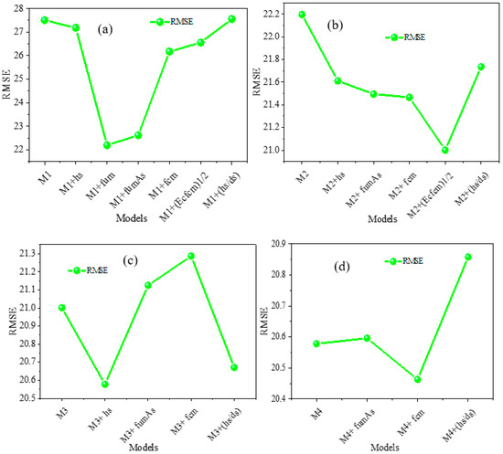
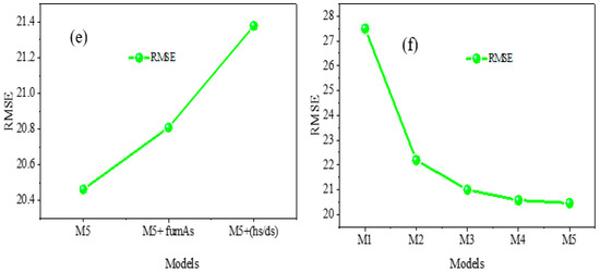
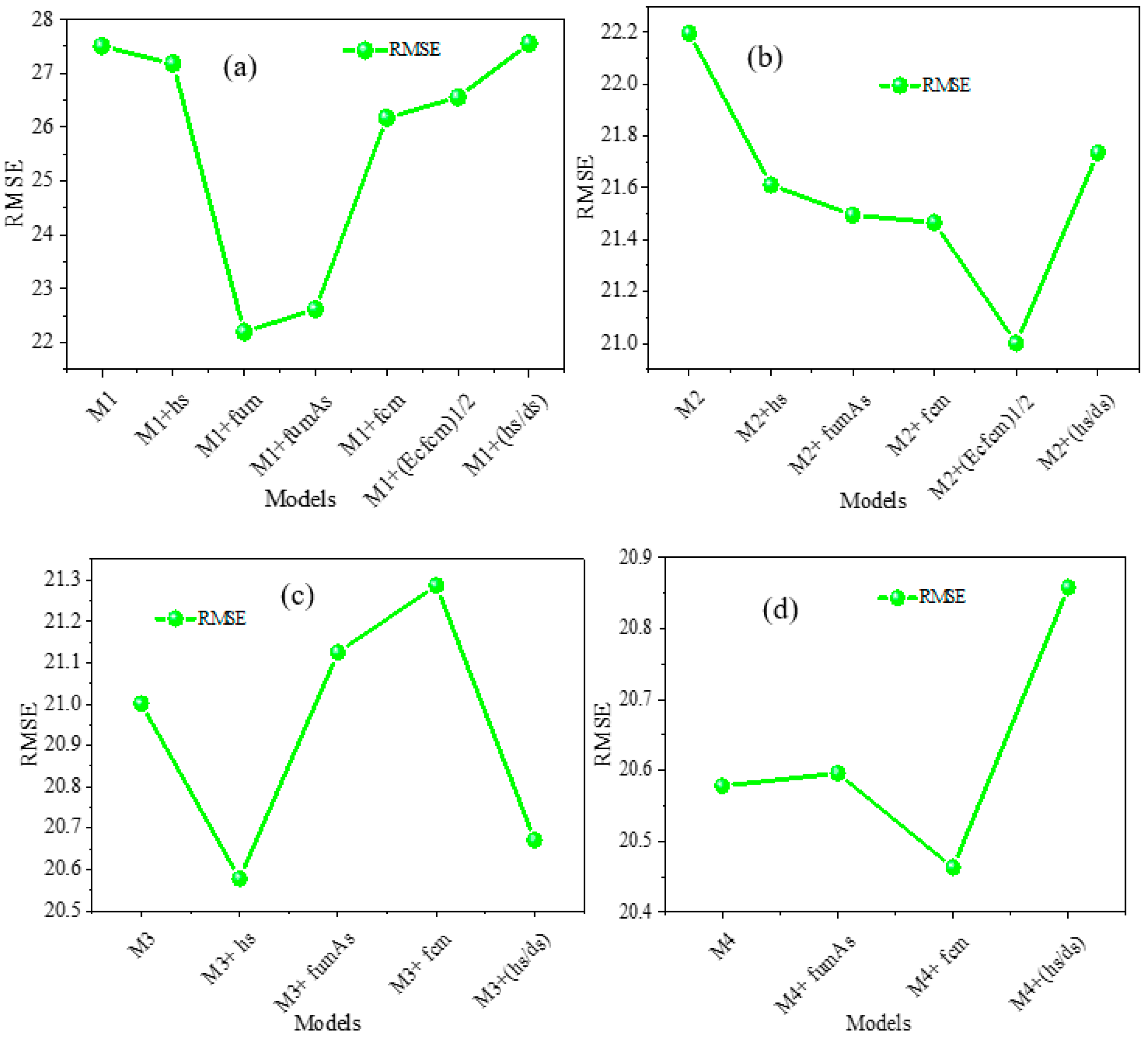
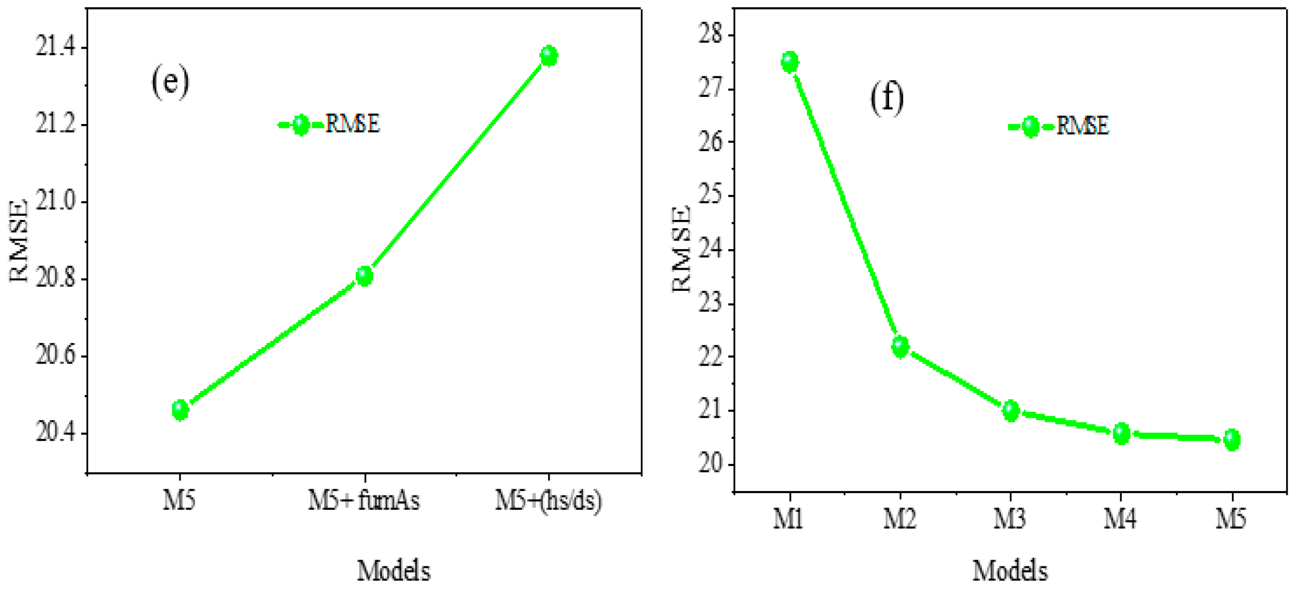
Various methodologies, such as the Akaike Information Criteria [56], Bayesian Information Criteria [57], backward elimination [58], Mallow coefficient [59], and ANFIS [60], have been suggested for identifying the set of input variables that exert control. Neural networks (NNs) for system identification provide enhanced precision, adaptability, and expandability in comparison to conventional techniques, particularly in intricate and non-linear systems. It is crucial to carefully develop and train neural network models to ensure reliable and interpretable results. Neural networks are highly effective in machine learning because they can model intricate, nonlinear relationships in data. They automatically identify significant characteristics from unprocessed data, reducing the need for manual feature engineering. Their scalability enables efficient processing of large datasets by leveraging parallel computing to speed up training. Neural networks demonstrate strong adaptability to novel inputs and can apply learned knowledge to unfamiliar situations, while remaining resilient to interference. Learning hierarchical representations improves performance in activities such as image recognition and natural language processing. Neural networks facilitate comprehensive learning, streamline system design, and enable topology customization for various applications and domains. Neural networks are notable for their adaptability and efficiency in many machine learning tasks. All parameters were considered as possible input variables. The first relevant variables, including Ec, ds, As, dw, hw, and Aw, were selected to be the first model (M1). Four additional models, M2 to M5, were developed based on the RMSE obtained for M₁. After evaluating M1’s performance based on RMSE, each input variable, except the M1 parameters, was added, and the resulting RMSE was recorded, as shown in Figure 13a. The model with the least RMSE was selected as the M₂ model. The process is repeated for M₃, M₄, and M₅, as shown in Figure 13b–e. Figure 13f presents the performance of the developed models M₁-M_5. The system identification results indicate that individual correlations between the input and target variables are insufficient to capture the model’s performance; combining the input variables can significantly improve performance, as shown in Figure 13a. The PC and MI techniques indicate that the stud’s tensile strength (fu) is not a relevant parameter; however, combining it with other input variables makes fu more relevant. Table 7 summarizes the developed models and their performance, while Figure 13 presents the schematic representation of the system identification method.

$$SI=\left\{\begin{array}{c}{M}_1\\ M_1+h_s\\ (M_1+f_{um})=M_2\\ M_1+f_{um}{A}_s\\ M_1+f_{cm}\\ M_1+{(E_c{f}_{cm})}^{1/2}\\ M_1+({\displaystyle \raisebox{1ex}{$h_s$}\!\left/ \!\raisebox{-1ex}{$d_s$}\right.})\end{array}\right.\Rightarrow \left\{\begin{array}{c}{M}_2\\ M_2+h_s\\ M_2+f_{um}{A}_s\\ M_2+f_{cm}\\ \left[M_2+{(E_c{f}_{cm})}^{1/2}\right]=M_3\\ M_2+({\displaystyle \raisebox{1ex}{$h_s$}\!\left/ \!\raisebox{-1ex}{$d_s$}\right.})\end{array}\right.\Rightarrow \left\{\begin{array}{c}{M}_3\\ \left(M_3+h_s\right)=M_4\\ M_3+f_{um}{A}_s\\ M_3+f_{cm}\\ M_3+({\displaystyle \raisebox{1ex}{$h_s$}\!\left/ \!\raisebox{-1ex}{$d_s$}\right.})\end{array}\right.\Rightarrow \left\{\begin{array}{c}{M}_4\\ M_4+f_{um}{A}_s\\ \left(M_4+f_{cm}\right)=M_5\\ M_4+({\displaystyle \raisebox{1ex}{$h_s$}\!\left/ \!\raisebox{-1ex}{$d_s$}\right.})\end{array}\right.\Rightarrow \left\{\begin{array}{c}{M}_5\\ M_4+f_{um}{A}_s\Rightarrow \left\{M_5\right.\\ M_4+({\displaystyle \raisebox{1ex}{$h_s$}\!\left/ \!\raisebox{-1ex}{$d_s$}\right.})\end{array}\right.$$

Figure 13. System identification results for model combination: (a) M1, (b) M2, (c) M3, (d) M4, (e) M4, (f) RMSE of all models.

Table 7. Model development.

MODEL	RMSE	MODEL	RMSE	MODEL	RMSE	MODEL	RMSE	MODEL	RMSE
M1	27.500	M2	22.195	M3	21.001	M4	20.578	M5	20.463
M1 + hs	27.176	M2 + hs	21.611	M3 + hs	20.578	-	-	-	-
M1 + fum	22.195	-	-	-	-	-	-	-	-
M1 + fumAs	22.619	M2 + fumAs	21.495	M3 + fumAs	21.125	M4 + fumAs	20.596	M5 + fumAs	20.809
M1 + fcm	26.168	M2 + fcm	21.466	M3 + fcm	21.287	M4 + fcm	20.463	-	-
M1 + (Ecmfcm)1/2	26.550	M2 + (Ecfcm)1/2	21.001	-	-	-	-	-	-
M1 + (hs/ds)	27.549	M2 + (hs/ds)	21.735	M3 + (hs/ds)	20.671	M4 + (hs/ds)	20.858	M5 + (hs/ds)	21.379

Five models (M1–M5) according to system identification result were developed and trained using six ML algorithms, including ANN, MLR, SVM, ELM, DT, and hybrid ANN-PSO. The performance of these models during training and testing was summarized in Table 6 using statistical metrics. As shown in Table 8, the R² values at the training stage are higher than those at the testing stage, and the lower and higher values of MAE, RMSE, and MAPE are observed at the training and testing stages, respectively. These statistical indicators quantify the discrepancy between the observed and predicted values. Lower MAE, RMSE, and MAPE values indicate stronger predictive performance, whereas higher R² values indicate better performance. As noted in Table 8, all ML algorithms achieved high accuracy in predicting shear strength at both the training and test stages, with R² values exceeding 80%. Moreover, the hybrid ANN-PSO model achieved the best performance, with R² = 0.976, MAE = 7.61 kN, RMSE = 10.8 kN, and MAPE = 8.04 kN, demonstrating the highest prediction accuracy among the classical models. The ANN-PSO achieves the highest prediction accuracy by analytically optimizing the ANN parameters (biases and weights) using PSO to update particle positions. This result agrees with previous studies [22,61], which reported that PSO improves ANN performance. On the other hand, DT is the second-best model for predicting the shear strength of stud connectors based on system identification of input parameters. The models had R² = 0.958, MAE = 10.27 kN, RMSE = 14.43 kN, and MAPE = 8.53 kN. These selected models revealed nearly equal performance for predicting the shear capacity of stud connectors embedded in concrete. Therefore, based on the outcomes of the developed models, it was observed that systematically identifying input parameters for model development yields promising results.

Table 8. The performance indicators.

Model	Phase	R2	MAE	RMSE	MAPE
ANN	Training	0.897	15.598	21.611	13.731
	Testing	0.802	32.242	37.620	24.500
MLR	Training	0.884	18.601	25.746	16.297
	Testing	0.879	22.278	26.656	17.843
SVM	Training	0.894	16.110	24.574	13.265
	Testing	0.899	18.557	24.311	13.999
ELM	Training	0.839	22.689	30.277	18.737
	Testing	0.860	24.982	28.639	20.980
DT	Training	0.958	10.270	14.427	8.526
	Testing	0.887	19.041	26.036	14.517
ANN-PSO	Training	0.976	7.610	10.801	8.043
	Testing	0.927	15.560	20.668	16.149

3.5. Model Validation

The validation follows a two-step sequence. The complete dataset was split into 70% for training and 30% for testing. This allows the models to be evaluated on data they have never seen before. For the training section, a 10-fold cross-validation was employed to facilitate hyperparameter tuning, model selection, and overfitting control. As a result of cross-validation, the parameters were optimized. At the same time, 30% of the data was held out as a test set to evaluate the final model performance in a truly unbiased way. This clear sequence of activities resolves the prior uncertainty and enables all models to be validated in the same manner. The mean and standard deviation of R², RMSE, and MAE are now reported in Table 9.

Table 9. 10-fold CV statistics.

Model	CV Mean R2	CV Std R2	CV Mean RMSE (kN)	CV Std RMSE	CV Mean MAE (kN)	CV Std MAE
ANN	0.865	0.028	26.9	2.4	18.3	1.9
MLR	0.842	0.031	29.8	2.7	20.4	2.1
DT	0.901	0.065	24.2	4.8	16.7	3.5
SVM	0.915	0.022	22.6	1.9	15.1	1.4
ELM	0.872	0.035	27.4	3.0	19.5	2.3
ANN–PSO	0.944	0.018	18.9	1.5	12.8	1.1

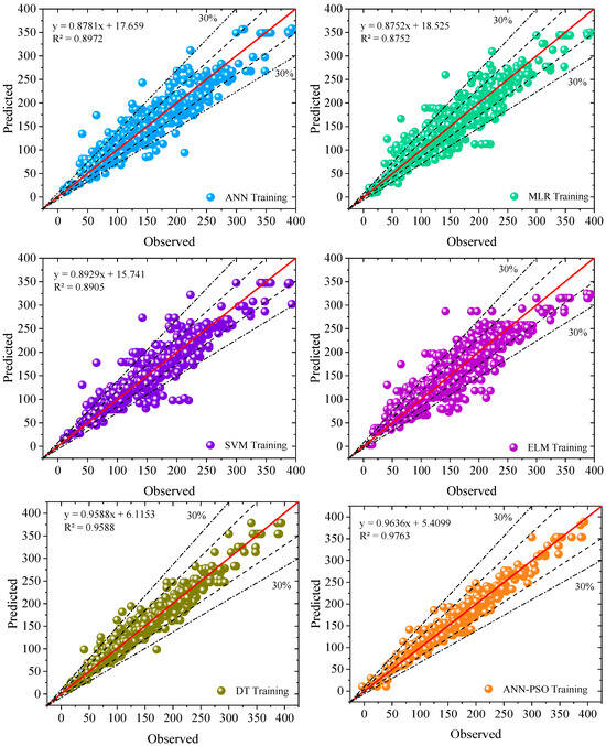
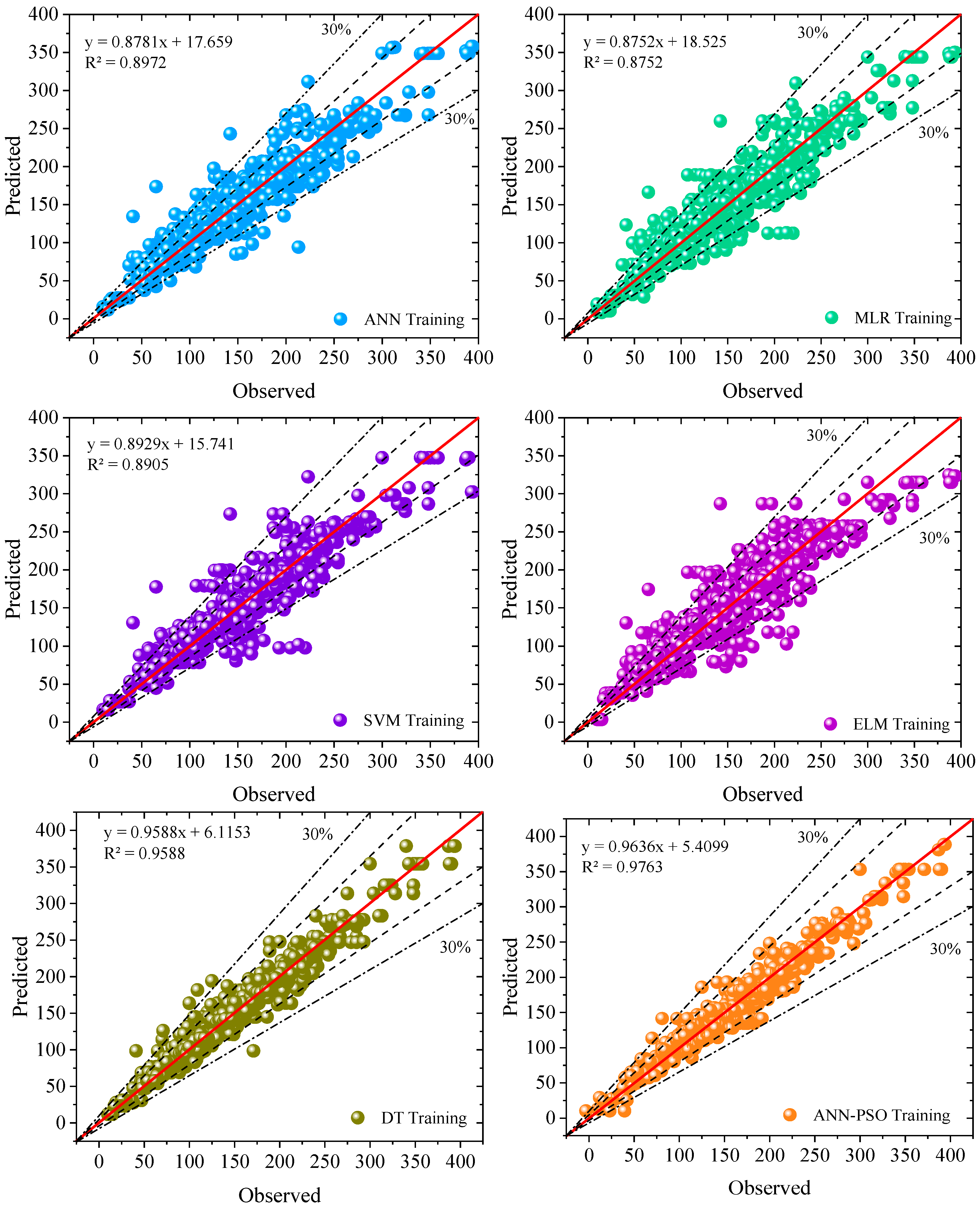
Figure 14 shows scatter plots of the measured and estimated shear resistance values during the training stage for the six developed models. As shown in Figure 13, the data points have clustered along the lines of fitness of the developed models, indicating a higher goodness-of-fit. The ML algorithm’s prediction accuracy was assessed by comparing the R² values of the developed models during training and testing, as depicted in Figure 14 and Figure 15, respectively. Better prediction accuracy was achieved among the developed models. The hybrid ANN-PSO model outperformed the classical models, achieving an R² value greater than those of ANN, MLR, SVM, ELM, and DT at the training stage by 8.81%, 10.41%, 9.17%, and 1.88%, respectively. The results indicate that the shear capacity of stud connectors can be calculated with minimal error using ML algorithms that incorporate several input parameters.

Figure 14. Scatter plot between the predicted and observed values of shear strength at the training phase.

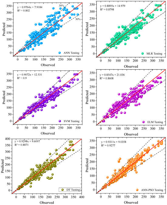
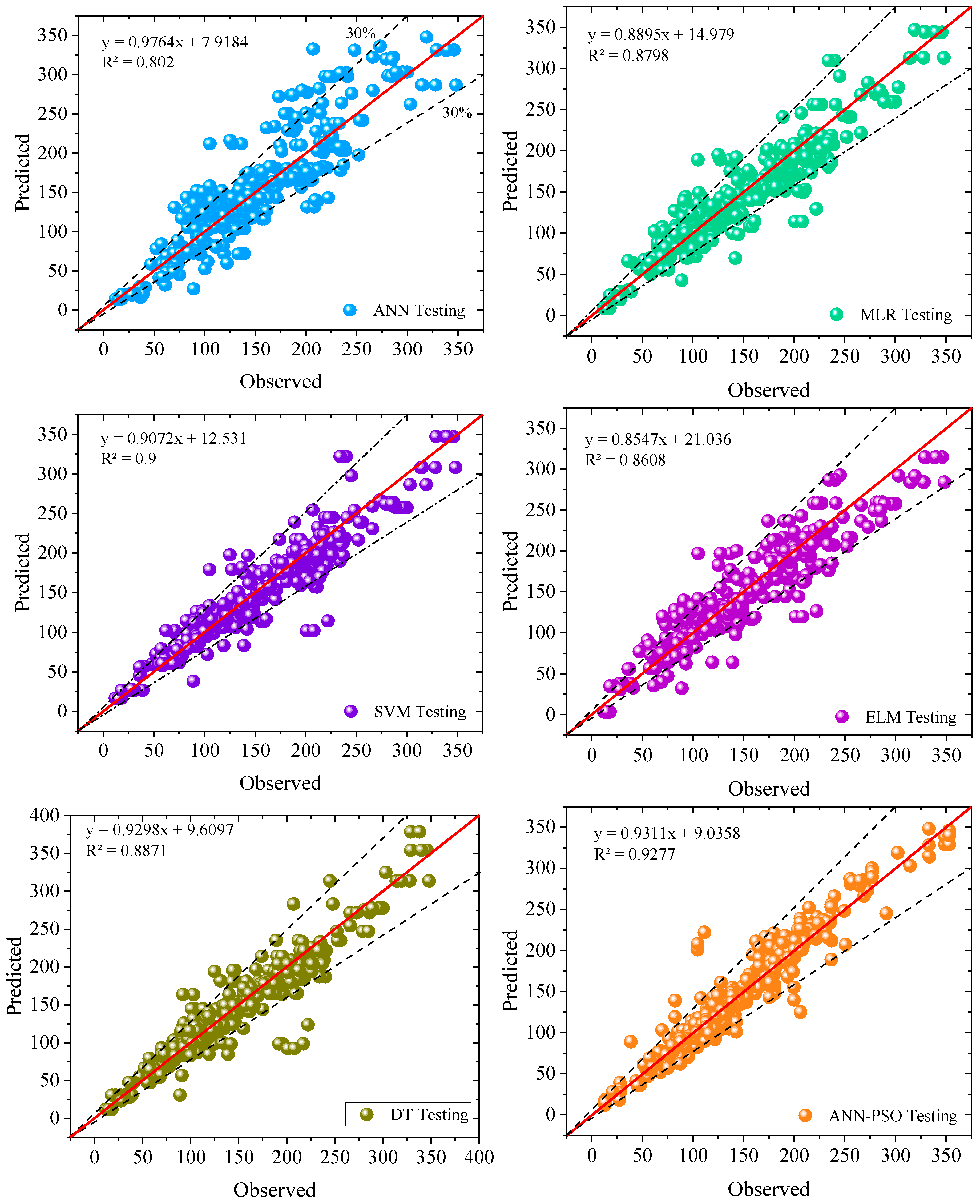
Figure 15. Scatter plot between the predicted and observed values of shear strength at the testing phase.

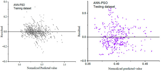
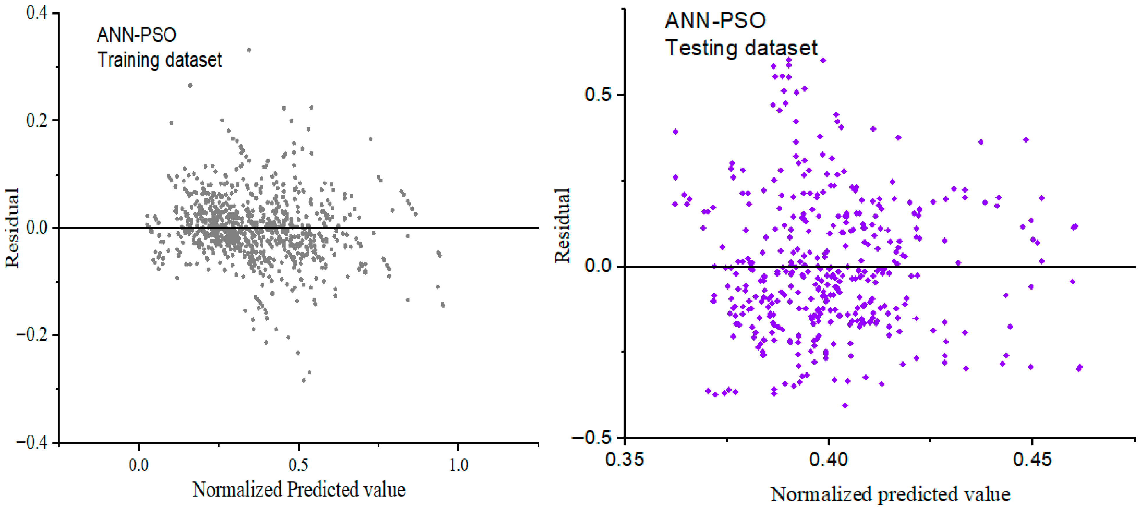
The scatter plot of the observed and predicted shear strength values at the testing stage is shown in Figure 15. Generally, the testing dataset results are lower than those of the training datasets for all the developed models, except for SVM, ELM, and DT, which show higher prediction accuracy at the testing stage. Similarly, ANN-PSO outperformed the other models in the test set, achieving an R² of 0.927, followed by SVM with an R² of 0.899. (See Figure 15). The prediction accuracy at the test stage ranged from 80 to 90%, and the ANN model was the least accurate in predicting shear strength in this study. Table 10 compares the model results from this study with those from the existing model developed in past studies that investigated the shear strength of steel-to-concrete composites. Figure 16 shows a residual plot of the ANN-PSO model, which achieved the best performance on the training and test datasets. The residuals plot demonstrated the difference between the predicted and actual responses.

Table 10. Comparison of model outcomes with developed ML models from previous studies.

Study	Model	Training Dataset					Testing Dataset
		MAE	RMSE	MAPE	R2	R	MAE	RMSE	MAPE	R2	R
Eurocode 4 [13]		-	-	-	-	-	38.8	43.5	-	0.32	-
Ref. [28]	LR	15.5	20.2	-	0.87	-	12.9	15.6	-	0.91	-
	DT	14.7	20.6	-	0.87	-	13.2	19.9	-	0.86	-
	BET	11.9	16.5	-	0.92	-	11.6	18.1	-	0.88	-
	SVM	10.2	16.0	-	0.92	-	9.7	12.1	-	0.95	-
	GPR	10.7	15.7	-	0.92	-	9.1	15.2	-	0.92	-
	ANN	12.9	20.6	-	0.87	-	9.9	15.9	-	0.91	-
Ref. [62]	ANN	17.8	26.8	12.8	0.91	-	21.7	34.9	23.9	0.85	-
	ELM	20.1	28.4	15.6	0.89	-	24.9	35.8	35.5	0.84	-
	ANFIS	6.2	12.8	3.7	0.94	-	16.3	28.6	16.2	0.90	-
Ref. [27]	EN	25.6	34.1	26.2	-	0.9	25.7	34.1	26.4	-	0.9
	BR	18.5	25.4	16.6	-	0.93	18.8	25.6	16.8	-	0.93
	DNN	11.5	15.4	10.1	-	0.97	13.3	17.9	11.8	-	0.96
	LightGBM	12.8	17.6	12.6	-	0.97	14.7	20.4	14.5	-	0.95
	GP-LightGBM	4.8	7.7	3.8	-	0.99	10.8	15.6	8.9	-	0.97
	PRF-LightGBM	5.2	8.0	4.1	-	0.99	10.5	15.3	8.8	-	0.97
Current study	ANN	15.6	21.6	13.7		-	32.24	37.62	24.50	0.80	-
	MLR	18.60	25.75	16.29	0.89	-	22.28	26.66	17.84	0.88	-
	SVM	16.11	24.57	13.27	0.89	-	18.56	24.31	13.99	0.89	-
	ELM	22.69	30.28	18.74	0.84	-	24.98	28.64	20.98	0.86	-
	DT	10.27	14.43	8.54	0.96	-	19.04	26.04	14.52	0.89	-
	ANN-PSO	7.61	10.80	8.04	0.98	-	15.56	20.67	16.15	0.93	-

Figure 16. Residual plot vs. normalized predicted value for ANN-PSO.

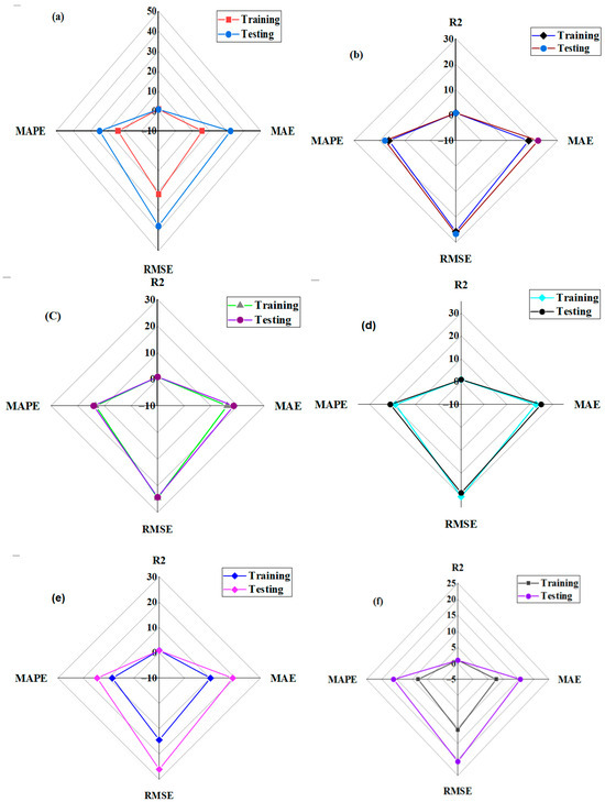
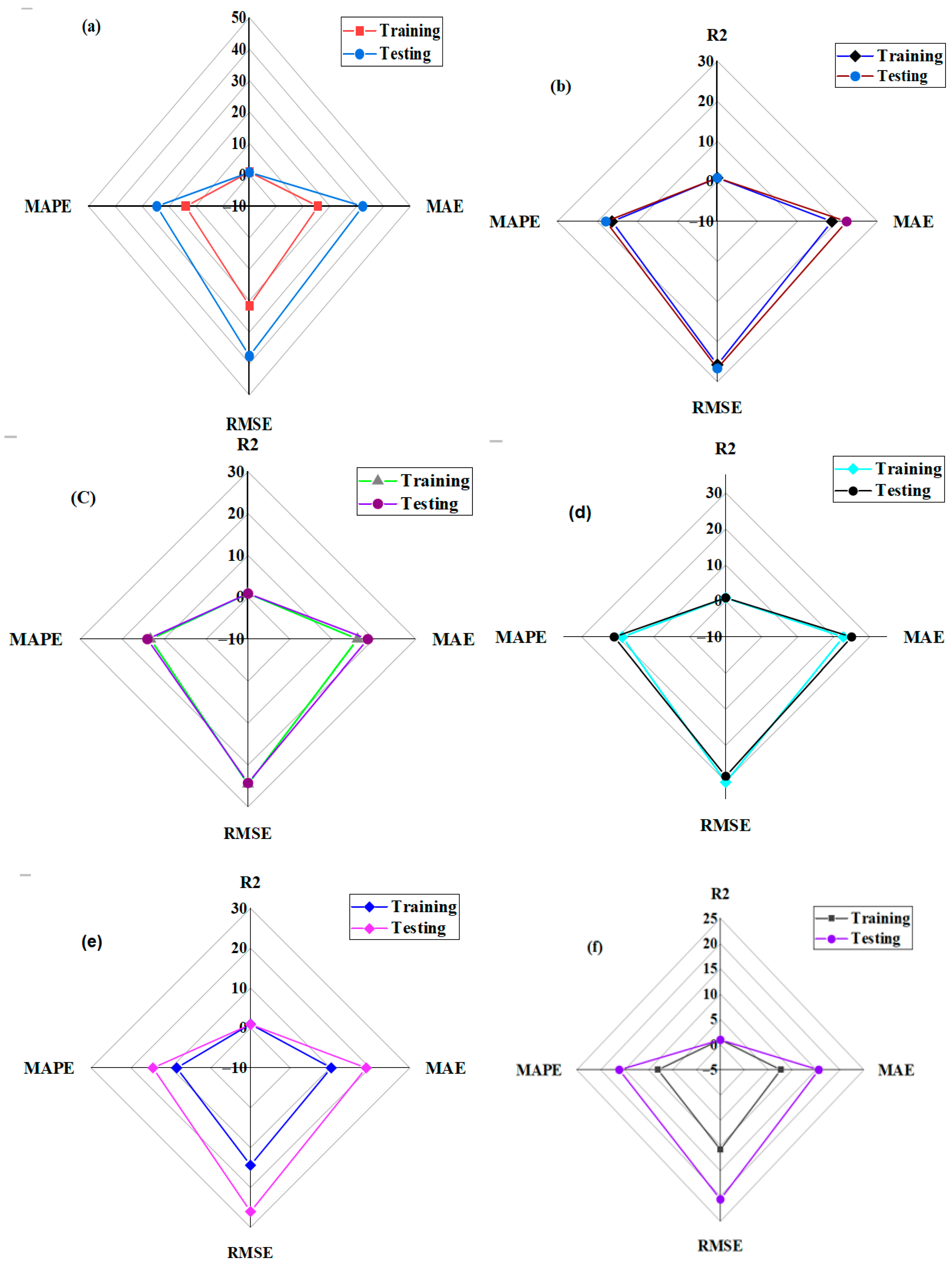
Figure 17 shows a radar plot comparing the performance of the developed model during training and testing. The plots demonstrate the performance matrices obtained at the two modeling stages. As shown in Figure 17a–f, the training datasets exhibit lower MAPE, RMSE, and MAE, and higher R², than those at the test stage, indicating that all the developed models performed better during training. The variation in model performance between training and testing is more pronounced for the ANN, DT, and ANN-PSO models, as shown in Figure 17a and Figure 17e, and Figure 17f, respectively.

Figure 17. The radar plot compares the model performance indicator at the modeling stage: (a) ANN, (b) MLR, (c) SVM, (d) ELM, (e) DT, and (f) ANN-PSO models.

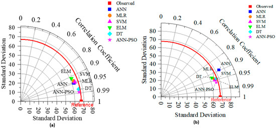
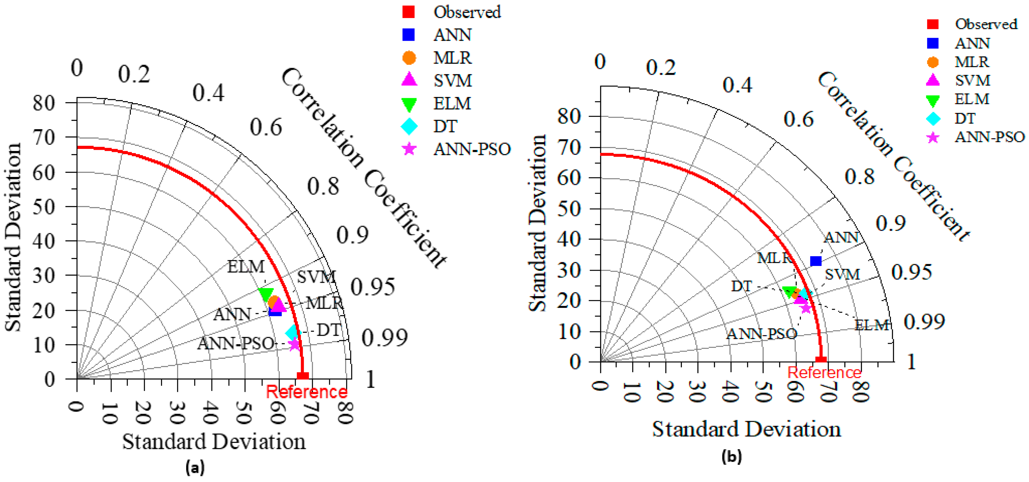
Furthermore, the six (6) developed models (ANN, MLR, SVM, ELM, DT, and ANN-PSO) were also evaluated using the 2D Taylor diagram (Figure 18), which illustrates the observed and output features [63]. The Taylor diagram was endorsed for accuracy appraisal [64]. Two measurements, the standard deviation (SD) and the correlation (R), were combined to create a Taylor diagram [65]. The core objectives of the diagram are to assess the agreement between experimental shear strength and predicted values, and to evaluate multiple performance measures in a single combination. It can be observed in (Figure 18a,b) that the best performance results were achieved by the ANN-PSO technique with R-value = 0.979 at the training stage. The specified indicator reflects the ANN-PSO’s forecast accuracy. Because the computed values were more closely aligned with the observed locations, ANN-PSO outperformed the other models. The high SD value, which may be related to the ANN-PSO, provides additional evidence. Overestimation typically occurs when the SD of the calculated values exceeds that of the observed values, and vice versa.

Figure 18. Taylor diagram illustrating the model performance: (a) training and (b) testing stage.

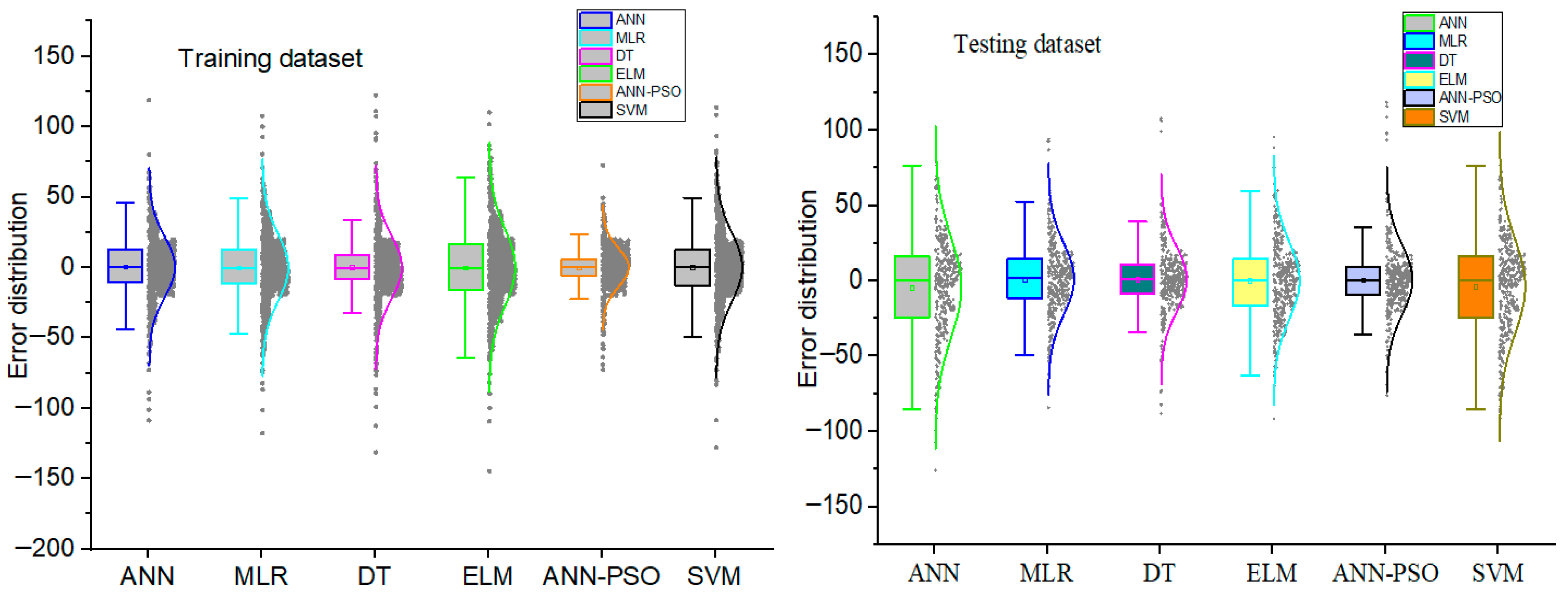
Figure 19 shows the error distributions of the developed ANN, MLR, SVM, DT, and ANN-PSO models during training and testing stages. The minimum and maximum errors of the distribution are computed during the training phase for the DT and ANN-PSO models. Similarly, minimum and maximum error distributions were calculated during the testing phase of the DT and ANN-PSO models. Overall, all models predicted shear capacity with a reasonable distribution of errors.

Figure 19. Boxplot illustrating error distribution.

4. Conclusions

In this study, the shear resistance of a headed stud fixed in concrete was accurately predicted using both classical and hybrid models. A large database from the experimental push-out tests for stud connectors in concrete will be collected from the literature. The models were trained in diverse input features, which were systematically incorporated via a system identification technique. The ML algorithms employed to train the shear strength database include ANN, MLR, SVM, ELM, DT, and ANN-PSO. Feature selection methods and system identification were applied to identify optimal or most relevant input parameters.

(1)

The feature selection based on the Pearson correlation matrix and the mutual information system showed that the dimensional features (ds, dw, and As) are the most relevant variables with the MI values of 0.322, 0.309, and 0.299, respectively. Therefore, the study considered the results of the two feature selection techniques, which revealed that E_cm, ds, As, dw, hw, and Aw are the most relevant input variables.

(2)

The system identification involved all twelve (12) parameters as potential input variables for estimating the shear resistance of the stud connector. The first most relevant variables, including E_cm, ds, As, dw, hw, and Aw, were selected to be the first developed model (M1), and other models, such as M2 to M5, were developed based on the RMSE result obtained from the M1.

(3)

The five models (M1–M5) according to system identification result were developed and trained the ML algorithms, including ANN, MLR, SVM, ELM, DT, and hybrid ANN-PSO. The ANN-PSO model outperformed the other classical models in estimating the shear capacity of headed stud connectors at both the training and testing stages.

(4)

The result obtained indicates that the shear strength of stud connectors can be evaluated with minimum error using the ML algorithms involving several input parameters, which exhibit linear and nonlinear interactions with the target parameter. The hybrid ANN-PSO achieved R² = 0.976, MAE = 7.61 kN, RMSE = 10.8 kN, and MAPE = 8.04 MPa, demonstrating the best prediction accuracy among the classical models. On the other hand, DT is the second-best model, with an R² of 0.958, an MAE of 10.27 kN, an RMSE of 14.43 kN, and an MAPE of 8.53 kN for forecasting shear capacity.

(5)

The integration of hybrid ANN-PSO techniques into neural network frameworks demonstrated remarkable improvement over standalone ML models, advancing improved parameter tuning and reduced reliance on experimental testing. Broad applications in the construction industry, where accurate predictions of stud connectors in the composites section can inform compliance with standard codes, optimize the stud’s fabrication, and support the implementation of eco-friendly materials for structural engineering. Uncertainty quantification via Bayesian approaches or Monte Carlo simulations to quantify prediction uncertainties, improving reliability in safety-critical scenarios, is recommended for future study.

References

- Wu, F.; Tang, W.; Liu, S.; Fan, Z.; Yang, F. Shear behaviours of steel-HSFRC welded stud and perfobond rib connectors under static push-out experiments. Structures 2023, 54, 1101–1113. [Google Scholar] [CrossRef] [Scilit]
- Tong, L.; Chen, L.; Wen, M.; Xu, C. Static behavior of stud shear connectors in high-strength-steel–UHPC composite beams. Eng. Struct. 2020, 218, 110827. [Google Scholar] [CrossRef] [Scilit]
- Nawar, M.T.; El-Zohairy, A.; Maaly, H.M.; Husain, M.; Salama, I.; Mousa, E. Prestressed steel-concrete composite I-beams with single and double corrugated web. Buildings 2023, 13, 647. [Google Scholar] [CrossRef] [Scilit]
- Benedetty, C.A.; dos Santos, V.B.; Krahl, P.A.; Rossi, A.; de Andrade Silva, F.; Cardoso, D.C.T.; Martins, C.H. Flexural and shear behavior of steel-UHPC composite beams: A review. Eng. Struct. 2023, 293, 116649. [Google Scholar] [CrossRef] [Scilit]
- Pardeshi, R.T.; Patil, Y.D. Review of various shear connectors in composite structures. Adv. Steel Constr. 2021, 17, 394–402. [Google Scholar]
- Ding, F.; Yin, G.; Wang, H.; Wang, L.; Guo, Q. Static behavior of stud connectors in bi-direction push-off tests. Thin-Walled Struct. 2017, 120, 307–318. [Google Scholar] [CrossRef] [Scilit]
- Kumar, P.; Chaudhary, S. Effect of reinforcement detailing on performance of composite connections with headed studs. Eng. Struct. 2019, 179, 476–492. [Google Scholar] [CrossRef] [Scilit]
- Shim, C.-S.; Lee, P.-G.; Kim, D.-W.; Chung, C.-H. Effects of group arrangement on the ultimate strength of stud shear connection. In Composite Construction in Steel and Concrete VI; American Society of Civil Engineers: Reston, VA, USA, 2011; pp. 92–101. [Google Scholar]
- Ollgaard, J.G.; Slutter, R.G.; Fisher, J.W. Shear strength of stud connectors in lightweight and normal weight concrete. AISC Eng. J. 1971, 8, 55–64. [Google Scholar] [CrossRef] [Scilit]
- Driscoll, G.C.; Slutter, R.G. Research on composite design at Lehigh University, Proc. AISC, National Engineering Conference, (1961), Reprint No. 180 (61-8); Lehigh University: Bethlehem, PA, USA, 1961; pp. 18–24. Available online: https://preserve.lehigh.edu/lehigh-scholarship/faculty-and-staff-publications/fritz-lab-reports/research-composite-design (accessed on 1 January 2026).
- AISC. Load and Resistance Factor Design Specification for Structural Steel Buildings; American Institute of Steel Construction: Chicago, IL, USA, 1986. [Google Scholar]
- EN 1994-1-1; Eurocode 4: Design of Composite Steel and Concrete Structures. CEN-European Committee for Standardization: Brussels, Belgium, 2004.
- Roik, K.; Hanswille, G.; Cunze-O, L.A. Harmonisation of the European Construction Codes–Eurocode 2, 4 and 8/Part 3–Report on Eurocode 4 Clause 6.3. 2 Stud Connectors; Institute for Structural Engineering, Ruhr-Universität-Bochum: Bochum, Germany, 1989. [Google Scholar]
- Mirrashid, M.; Naderpour, H. Recent trends in prediction of concrete elements behavior using soft computing (2010–2020). Arch. Comput. Methods Eng. 2021, 28, 3307–3327. [Google Scholar] [CrossRef] [Scilit]
- Hosseinpour, M.; Sharifi, Y.; Sharifi, H. Neural network application for distortional buckling capacity assessment of castellated steel beams. Structures 2020, 27, 1174–1183. [Google Scholar] [CrossRef] [Scilit]
- Degtyarev, V. V Neural networks for predicting shear strength of CFS channels with slotted webs. J. Constr. Steel Res. 2021, 177, 106443. [Google Scholar] [CrossRef] [Scilit]
- Rahman, J.; Ahmed, K.S.; Khan, N.I.; Islam, K.; Mangalathu, S. Data-driven shear strength prediction of steel fiber reinforced concrete beams using machine learning approach. Eng. Struct. 2021, 233, 111743. [Google Scholar] [CrossRef] [Scilit]
- Abdulrahman, S.; Bashir, A.; Farouk, A.I.B.; Haruna, S.I.; Haruna, A.; Abba, S.I. Hybrid-optimized ensemble learning models and GUI for predicting compressive strength of fly ash and slag concrete. Mater. Today Commun. 2025, 49, 113762. [Google Scholar] [CrossRef] [Scilit]
- Asteris, P.G.; Plevris, V. Anisotropic masonry failure criterion using artificial neural networks. Neural Comput. Appl. 2017, 28, 2207–2229. [Google Scholar] [CrossRef] [Scilit]
- Tran, V.-L.; Thai, D.-K.; Nguyen, D.-D. Practical artificial neural network tool for predicting the axial compression capacity of circular concrete-filled steel tube columns with ultra-high-strength concrete. Thin-Walled Struct. 2020, 151, 106720. [Google Scholar] [CrossRef] [Scilit]
- Naser, M.Z.; Thai, S.; Thai, H.-T. Evaluating structural response of concrete-filled steel tubular columns through machine learning. J. Build. Eng. 2021, 34, 101888. [Google Scholar] [CrossRef] [Scilit]
- Farouk, A.I.B.; Zhu, J.; Ding, J.; Haruna, S.I. Prediction and uncertainty quantification of ultimate bond strength between UHPC and reinforcing steel bar using a hybrid machine learning approach. Constr. Build. Mater. 2022, 345, 128360. [Google Scholar] [CrossRef] [Scilit]
- Haruna, S.I.; Ibrahim, Y.E.; Abba, S.I. Prediction of the Ultimate Impact Response of Concrete Strengthened with Polyurethane Grout as the Repair Material. Infrastructures 2025, 10, 128. [Google Scholar] [CrossRef] [Scilit]
- Al-shawafi, A.; Zhu, H.; Laqsum, S.A.; Haruna, S.I.; Ibrahim, Y.E. Improved static and impact properties of UHPFRC retrofitted with PU grout materials: Experiments and ML algorithms. Results Eng. 2024, 23, 102655. [Google Scholar] [CrossRef] [Scilit]
- Haruna, S.I.; Ibrahim, Y.E.; Umar, I.K. Machine Learning Approach for Prediction and Reliability Analysis of Failure Strength of U-Shaped Concrete Samples Joined with UHPC and PUC Composites. J. Compos. Sci. 2025, 9, 23. [Google Scholar] [CrossRef] [Scilit]
- Wang, X.; Liu, Y.; Xin, H. Bond strength prediction of concrete-encased steel structures using hybrid machine learning method. Structures 2021, 32, 2279–2292. [Google Scholar] [CrossRef] [Scilit]
- Wang, X.; Liu, Y.; Chen, A.; Ruan, X. Auto-tuning ensemble models for estimating shear resistance of headed studs in concrete. J. Build. Eng. 2022, 52, 104470. [Google Scholar] [CrossRef] [Scilit]
- Razavi Setvati, M.; Hicks, S.J. Machine learning models for predicting resistance of headed studs embedded in concrete. Eng. Struct. 2022, 254, 113803. [Google Scholar] [CrossRef] [Scilit]
- EN 1994-1-1; Eurocode 2: Design of Concrete Structures: Part 1-1: General Rules and Rules for Buildings. British Standards Institution: London, UK, 2004.
- Wang, X.; Liu, Y. Database-Shear Resistance of Headed Studs in Concrete. Version 1; Mendeley Data. 2022. Available online: https://data.mendeley.com/datasets/c6d6zkvgnw/1 (accessed on 1 January 2026).
- Farouk, A.I.B.; Jinsong, Z. Prediction of Interface Bond Strength Between Ultra-High-Performance Concrete (UHPC) and Normal Strength Concrete (NSC) Using a Machine Learning Approach. Arab. J. Sci. Eng. 2022, 47, 5337–5363. [Google Scholar] [CrossRef] [Scilit]
- Nguyen, T.-A.; Ly, H.-B.; Pham, B.T. Backpropagation Neural Network-Based Machine Learning Model for Prediction of Soil Friction Angle. Math. Probl. Eng. 2020, 2020, 8845768. [Google Scholar] [CrossRef] [Scilit]
- Taffese, W.Z.; Espinosa-Leal, L. Prediction of chloride resistance level of concrete using machine learning for durability and service life assessment of building structures. J. Build. Eng. 2022, 60, 105146. [Google Scholar] [CrossRef] [Scilit]
- Costache, R.; Pham, Q.B.; Sharifi, E.; Linh, N.T.; Abba, S.I.; Vojtek, M.; Vojteková, J.; Nhi, P.T.; Khoi, D.N. Flash-Flood Susceptibility Assessment Using Multi-Criteria Decision Making and Machine Learning Supported by Remote Sensing and GIS Techniques. Remote Sens. 2020, 12, 106. [Google Scholar] [CrossRef] [Scilit]
- Jain, A.K.; Mao, J.; Mohiuddin, K.M. Artificial neural networks: A tutorial. Computer 1996, 29, 31–44. [Google Scholar] [CrossRef] [Scilit]
- Shariati, M.; Mafipour, M.S.; Mehrabi, P.; Zandi, Y.; Dehghani, D.; Bahadori, A.; Shariati, A.; Trung, N.T.; Salih, M.N.; Poi-Ngian, S. Application of Extreme Learning Machine (ELM) and Genetic Programming (GP) to design steel-concrete composite floor systems at elevated temperatures. Steel Compos. Struct. 2019, 33, 319–332. [Google Scholar]
- Prasad, B.K.R.; Eskandari, H.; Reddy, B.V.V. Prediction of compressive strength of SCC and HPC with high volume fly ash using ANN. Constr. Build. Mater. 2009, 23, 117–128. [Google Scholar] [CrossRef] [Scilit]
- Karlik, B.; Olgac, A.V. Performance analysis of various activation functions in generalized MLP architectures of neural networks. Int. J. Artif. Intell. Expert Syst. 2011, 1, 111–122. [Google Scholar]
- Dietterich, T.G. Ensemble methods in machine learning. In Multiple Classifier Systems; Springer: Berlin, Heidelberg, 2000; pp. 1–15. [Google Scholar]
- Vandewiele, G.; Janssens, O.; Ongenae, F.; De Turck, F.; Van Hoecke, S. Genesim: Genetic extraction of a single, interpretable model. arXiv 2016, arXiv:1611.05722. [Google Scholar] [CrossRef] [Scilit]
- Breiman, L.; Ihaka, R. Nonlinear Discriminant Analysis via Scaling and ACE; Department of Statistics, University of California Davis One Shields Avenue: Davis, CA, USA, 1984. [Google Scholar]
- Çevik, A.; Kurtoğlu, A.E.; Bilgehan, M.; Gülşan, M.E.; Albegmprli, H.M. Support vector machines in structural engineering: A review. J. Civ. Eng. Manag. 2015, 21, 261–281. [Google Scholar] [CrossRef] [Scilit]
- Boser, B.E.; Guyon, I.M.; Vapnik, V.N. A Training Algorithm for Optimal Margin Classifiers. In COLT ’92: Proceedings of the Fifth Annual Workshop on Computational Learning Theory; Association for Computing Machinery: New York, NY, USA, 1992; pp. 144–152. [Google Scholar] [CrossRef] [Scilit]
- Huang, G.-B.; Zhu, Q.-Y.; Siew, C.-K. Extreme learning machine: Theory and applications. Neurocomputing 2006, 70, 489–501. [Google Scholar] [CrossRef] [Scilit]
- Zhang, Y.; Qiu, J.; Zhang, Y.; Wei, Y. The adoption of ELM to the prediction of soil liquefaction based on CPT. Nat. Hazards 2021, 107, 539–549. [Google Scholar] [CrossRef] [Scilit]
- Shariati, M.; Trung, N.T.; Wakil, K.; Mehrabi, P.; Safa, M.; Khorami, M. Estimation of moment and rotation of steel rack connections using extreme learning machine. Steel Compos. Struct. 2019, 31, 427–435. [Google Scholar]
- Al-Shamiri, A.K.; Kim, J.H.; Yuan, T.-F.; Yoon, Y.S. Modeling the compressive strength of high-strength concrete: An extreme learning approach. Constr. Build. Mater. 2019, 208, 204–219. [Google Scholar] [CrossRef] [Scilit]
- Kennedy, J.E. Particle swarm optimization. In Proceedings of the ICNN’95—International Conference on Neural Networks, Perth, WA, Australia, 27 November–1 December 1995; pp. 1942–1948. [Google Scholar]
- Qi, C.; Fourie, A.; Chen, Q. Neural network and particle swarm optimization for predicting the unconfined compressive strength of cemented paste backfill. Constr. Build. Mater. 2018, 159, 473–478. [Google Scholar] [CrossRef] [Scilit]
- Nourani, V.; Sharghi, Z.A.E. Sensitivity analysis and ensemble artificial intelligence-based model for short-term prediction of NO2 concentration. Int. J. Environ. Sci. Technol. 2020, 18, 2703–2722. [Google Scholar] [CrossRef] [Scilit]
- Nourani, V.; Khanghah, T.R.; Baghanam, A.H. Application of entropy concept for input selection of wavelet-ANN based rainfall-runoff modeling. J. Environ. Inform. 2015, 26, 52–70. [Google Scholar] [CrossRef] [Scilit]
- Wang, X.; Liu, Y.; Lu, Y.; Li, X. Shear transfer mechanism of perforated web connection for concrete encased steel structures. Eng. Struct. 2022, 252, 113418. [Google Scholar] [CrossRef] [Scilit]
- Wang, J.; Qi, J.; Tong, T.; Xu, Q.; Xiu, H. Static behavior of large stud shear connectors in steel-UHPC composite structures. Eng. Struct. 2019, 178, 534–542. [Google Scholar] [CrossRef] [Scilit]
- Rafindadi, A.D.; Ibrahim, Y.E.; Haruna, S.I.; Gora, A.M.; Kado, B. Assessing climate-resilient infrastructure design, implementation, and evaluation: A structural equation modeling approach. Results Eng. 2026, 29, 108692. [Google Scholar] [CrossRef] [Scilit]
- Sarstedt, M.; Ringle, C.M.; Hair, J.F. Partial Least Squares Structural Equation Modeling BT. In Handbook of Market Research; Homburg, C., Klarmann, M., Vomberg, A., Eds.; Springer International Publishing: Cham, Switzerland, 2017; pp. 1–40. [Google Scholar] [CrossRef] [Scilit]
- Sakamoto, Y.; Ishiguro, M.; Kitagawa, G. Akaike information criterion statistics. Dordr. Neth. D. Reidel 1986, 81, 26853. [Google Scholar]
- Chen, J.; Chen, Z. Extended Bayesian information criteria for model selection with large model spaces. Biometrika 2008, 95, 759–771. [Google Scholar] [CrossRef] [Scilit]
- Mao, K.Z. Orthogonal forward selection and backward elimination algorithms for feature subset selection. IEEE Trans. Syst. Man Cybern. Part B 2004, 34, 629–634. [Google Scholar] [CrossRef] [Scilit]
- Mallows, C.L. Some remarks of Cp. Technometrics 1973, 15, 661–675. [Google Scholar]
- Hou, Z.; Shen, Q.; Li, H. Nonlinear system identification based on ANFIS. In Proceedings of the International Conference on Neural Networks and Signal Processing, 2003. Proceedings of the 2003, Nanjing, China, 14–17 December 2003; Volume 1, pp. 510–512. [Google Scholar] [CrossRef] [Scilit]
- Alanazi, F.; Umar, I.K.; Haruna, S.I.; El-Kady, M.; Azam, A. Development of Artificial Intelligence Based Safety Performance Measures for Urban Roundabouts. Sustainability 2023, 15, 11492. [Google Scholar] [CrossRef] [Scilit]
- Yosri, A.M.; Farouk, A.I.B.; Haruna, S.I.; Deifalla, A.F.; Shaaban, W.M. Sensitivity and robustness analysis of adaptive neuro-fuzzy inference system (ANFIS) for shear strength prediction of stud connectors in concrete. Case Stud. Constr. Mater. 2023, 18, e02096. [Google Scholar] [CrossRef] [Scilit]
- Yaseen, Z.M.; Ebtehaj, I.; Kim, S.; Sanikhani, H.; Asadi, H.; Ghareb, M.I.; Bonakdari, H.; Wan Mohtar, W.H.; Al-Ansari, N.; Shahid, S. Novel Hybrid Data-Intelligence Model for Forecasting Monthly Rainfall with Uncertainty Analysis. Water 2019, 11, 502. [Google Scholar] [CrossRef] [Scilit]
- Zhu, S.; Heddam, S.; Wu, S.; Dai, J.; Jia, B. Extreme learning machine-based prediction of daily water temperature for rivers. Environ. Earth Sci. 2019, 78, 202. [Google Scholar] [CrossRef] [Scilit]
- Taylor, K.E. Summarizing multiple aspects of model performance in a single diagram. J. Geophys. Res. 2001, 106, 7183–7192. [Google Scholar] [CrossRef] [Scilit]
Disclaimer/Publisher’s Note: The statements, opinions and data contained in all publications are solely those of the individual author(s) and contributor(s) and not of MDPI and/or the editor(s). MDPI and/or the editor(s) disclaim responsibility for any injury to people or property resulting from any ideas, methods, instructions or products referred to in the content. |
© 2026 by the authors. Licensee MDPI, Basel, Switzerland. This article is an open access article distributed under the terms and conditions of the Creative Commons Attribution (CC BY) license.