Comparative Evaluation of Reinforcement Learning Algorithms for Multi-Agent Unmanned Aerial Vehicle Path Planning in 2D and 3D Environments

Abstract

Path planning in multi-agent UAV swarms is a crucial issue that involves avoiding collisions in dynamic, obstacle-filled environments while consuming the least amount of time and energy possible. This work comprehensively evaluates reinforcement learning (RL) algorithms for multi-agent UAV path planning in 2D and 3D simulated environments. First, we develop a 2D simulation setup using Python in which UAVs (quadcopters), represented as points in space, navigate toward their respective targets while avoiding static obstacles and inter-agent collisions. In the second phase, we transition this comparison to a physics-based 3D simulation, incorporating realistic UAV (fixed wing) dynamics and checkpoint-based navigation. We compared five algorithms, namely, Proximal Policy Optimization (PPO), Soft Actor–Critic (SAC), Deep Deterministic Policy Gradient (DDPG), Trust Region Policy Optimization (TRPO), and Multi–Agent DDPG (MADDPG), in various scenarios. Our findings reveal significant performance differences between the algorithms across multiple dimensions. DDPG consistently demonstrated superior reward optimization and collision avoidance performance, while PPO and MADDPG excelled in the execution time required to reach the goal. Furthermore, our findings reveal how algorithms perform while transitioning from a simplistic 2D setup to a realistic 3D physics-based environment, which is essential for performing sim-to-real transfer. This work provides valuable insights into the suitability of several reinforcement learning (RL) algorithms for developing autonomous systems and UAV swarm navigation.

1. Introduction

The use of unmanned aerial vehicles (UAVs) in swarm configurations has received significant attention in recent years due to their vast potential in diverse applications such as disaster management [1], rescue operations [2], surveillance [3], environmental mapping [4], logistics [5], and military operations [6]. With their ability to collaborate and perform complex tasks autonomously, UAV swarms present a scalable and cost-effective solution to address large-scale challenges. However, their deployment in real-world scenarios introduces complex problems such as communication constraints and environmental uncertainty, particularly in path planning [7].

Path planning in UAV swarms involves navigating multiple UAVs through dynamic and obstacle-rich environments to efficiently reach designated targets. Key challenges include obstacle avoidance and inter-agent collisions [8], optimizing flight time vis-à-vis energy consumption [9], and making sure that the performance of the entire swarm remains generalizable under uncertain and unknown conditions [10]. Traditional algorithmic approaches often fall short in handling such high-dimensional and dynamic problems, especially when scaling to large swarms or transitioning to real-world scenarios, even for high-fidelity simulations.

RL has emerged as a promising solution for autonomous path planning [11], enabling UAVs to learn optimal navigation policies through repeated environmental interactions. Using RL, UAVs can adapt to unforeseen challenges, dynamically optimize their paths, and achieve effective collision avoidance, even in previously unobserved environments [12]. Despite significant progress, a systematic evaluation of RL algorithms is needed to understand their strengths and limitations across various scenarios.

This paper addresses the gap by conducting a comprehensive comparative analysis of RL algorithms for multi-agent UAV path planning in 2D and 3D simulated environments. Our work hypothesizes that no single RL algorithm is universally optimal across all multi-agent UAV path planning scenarios. Instead, we posit that context-specific factors (environmental dimensionality, obstacle density, swarm size, etc.) can influence the relative effectiveness of different approaches. Therefore, our primary objective is to evaluate and contrast the performance of five widely used RL algorithms (DDPG, SAC, PPO, TRPO, and MADDPG) across both 2D and 3D simulated environments. By doing so, we aim to uncover the suitability and tradeoffs of each algorithm under varying operational conditions. Specifically, our work realizes the following:

• Compares the performance of five RL algorithms—Proximal Policy Optimization (PPO), Soft Actor–Critic (SAC), Trust Region Policy Optimization (TRPO), Deep Deterministic Policy Gradient (DDPG), and Multi–Agent DDPG (MADDPG)—in a 2D Python-based environment.
• Transitions to a physics-based Unity 3D simulator to incorporate realistic UAV dynamics and evaluate all five algorithms in a more complex, checkpoint-based navigation scenario.
• Introduces novel evaluation metrics, including obstacle-hitting probability (OHP), average completion time (ACT), distance to goal (DTG), total distance covered (TDC), and average velocity (AV), to provide detailed information into algorithmic performance.
• Highlights the impact of transitioning from simplified 2D to realistic 3D environments, emphasizing the role of algorithmic adaptability.

While addressing the gap between abstract simulations and realistic modeling, our study provides preliminary guidance to researchers and practitioners developing autonomous UAV swarm systems. Table 1 highlights the strengths and weaknesses of all the algorithms as well as their performance characteristics based on qualitative observations and quantitative metrics.

Table 1. Comparative summary of the pros and cons of studied RL algorithms evaluated in both two-dimensional Python and three-dimensional Unity environments.

Algorithm	Pros	Cons
DDPG	- Smooth trajectories - Lowest obstacle-hitting probability - Efficient in dynamic scenarios - Quick convergence in training	- Sensitive to reward shaping - Overfits to deterministic patterns
SAC	- Balanced exploration and exploitation - Better at discovering alternate routes - Good performance retention across maps	- Occasional unnecessary deviations - Higher time and steps than DDPG
PPO	- Relatively stable training - Higher average velocity and efficiency	- Prone to local minima - Highest obstacle-hitting probability - Least efficient in trajectory length
TRPO	- Strong theoretical guarantees - Relatively stable performance - Performs well in high-dimensional spaces	- Computationally expensive - Slower convergence
MADDPG	- Explicit multi-agent interaction modeling - Centralized training - Better coordination in cooperative tasks	- Requires synchronized updates - Sensitive to the number of agents - Higher complexity and overhead

2. Related Work

The problem of UAV path planning has been extensively studied due to its importance in various applications, including disaster relief [13], surveillance [14], autonomous delivery [15], precision agriculture [16], and others. Conventional approaches used for UAV path planning fall into several categories, including rule-based systems [17], heuristic algorithms [18], optimization-based approaches (A*, Dijkstra, genetic algorithms) [19], and machine learning techniques [20]. While these methods have achieved varying degrees of success in static or semi-static environments, they struggle with adaptability and scalability under dynamic, multi-agent, obstacle-laden conditions.

2.1. Conventional Approaches

Traditional path planning methods are widely employed in UAV navigation, particularly for single-agent setups. The A* algorithm and variants (Theta* and Anytime Repairing A*) have been extensively used for UAV navigation in structured environments [21,22]. Similarly, Dijkstra’s algorithm has been applied to UAV routing scenarios requiring optimal path computation under dynamic conditions [23]. However, these graph-based algorithms suffer from computational inefficiencies in large-scale and dynamic environments. Sampling-based motion planning techniques, such as Rapidly Exploring Random Trees (RRT) [24] and its optimized version, RRT* [25], have also been utilized for UAV path planning. RRT-based methods effectively generate feasible paths in cluttered environments; however, they often struggle with achieving smooth paths and real-time execution. Metaheuristic optimization techniques, including Genetic Algorithms (GAs) [26], multiple approaches based on Particle Swarm Optimization (PSO) [27], and Ant Colony Optimization (ACO) [28], have been explored as well. These approaches offer robust alternatives but require extensive tuning of hyperparameters and can be computationally expensive in high-dimensional spaces.

2.2. Multi-Agent Path Planning

Path planning challenges become significantly more complex in multi-agent UAV systems [29]. Coordination strategies are required to ensure inter-agent collision avoidance and optimized resource allocation. Swarm intelligence algorithms, such as Artificial Potential Fields (APF) [30,31], have been explored for cooperative UAV navigation. While these approaches provide decentralized and scalable solutions, they often lack optimality and suffer from local minima problems. Auction-based [32] and consensus-based approaches [33] have also been proposed for decentralized swarm coordination. These methods dynamically allocate tasks among UAVs, thereby improving efficiency in task execution. However, they rely on strong inter-agent communication, which may not always be feasible in real-world deployments.

Recent work has also focused on hybrid frameworks that combine classical planning algorithms with deep learning-based policies for improved generalization [34]. Graph-based methods are increasingly used to encode agent relationships and communication constraints within multi-agent path planning frameworks [35]. Furthermore, research into conflict-based search (CBS) methods and priority-based planning has led to more scalable solutions for large swarms [36].

With the rise of simulation platforms like AirSim and Unity-based testbeds, learning-based approaches to cooperative navigation and collision avoidance in three-dimensional environments have become more accessible and reliable [37]. Still, challenges like non-stationarity and partial observability remain active areas of research. These factors significantly affect training stability and policy convergence, especially when agents are trained in a decentralized manner without access to global information.

2.3. Reinforcement Learning

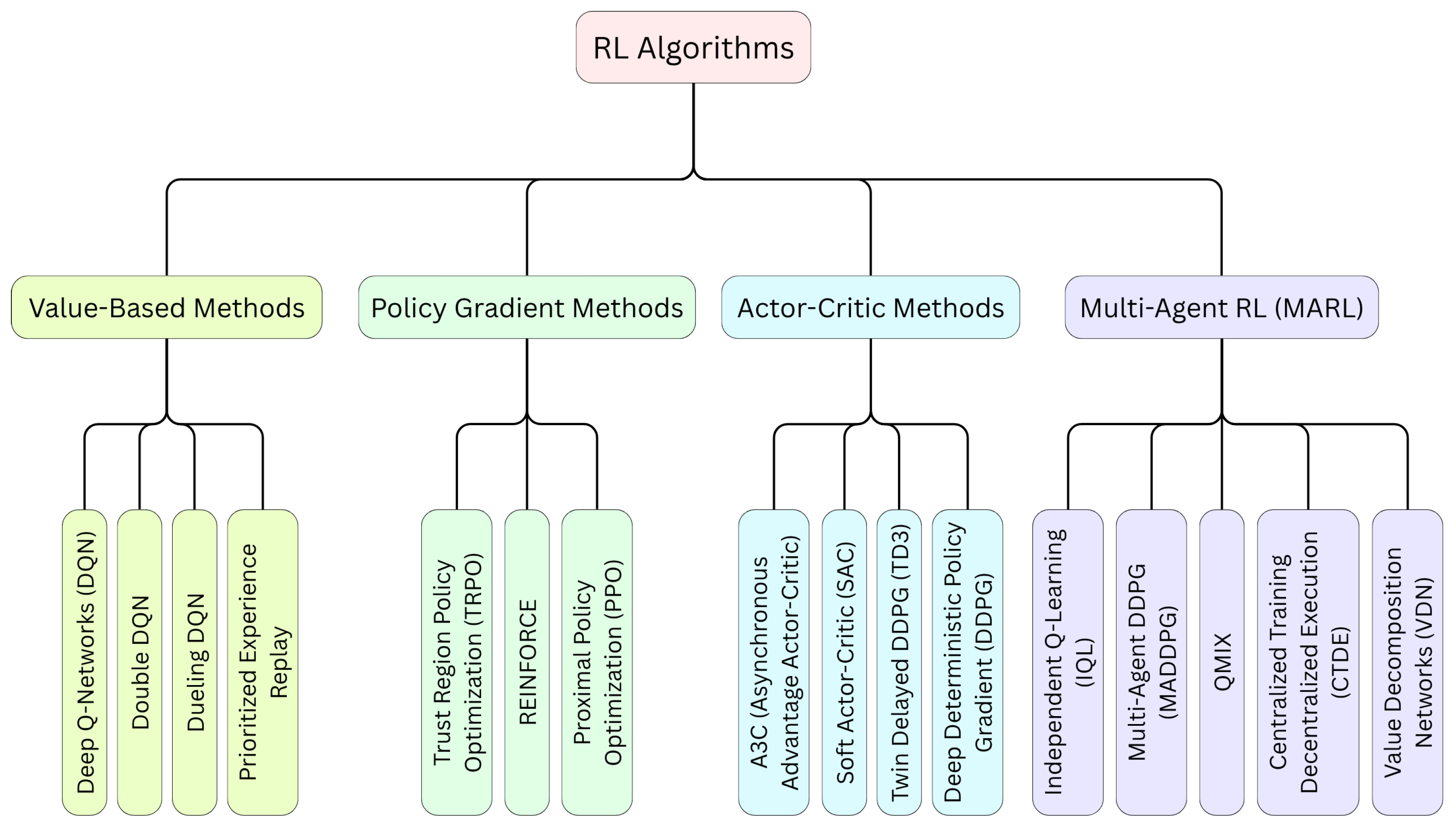
A promising approach to autonomous UAV path planning is reinforcement learning (RL) [38], offering the ability to learn optimal navigation policies through continuous environmental interaction. RL encompasses a wide spectrum of algorithms and methodologies, each with distinct mathematical foundations and application contexts. The broader landscape of RL methods is summarized in Figure 1 as a taxonomy diagram. We briefly review the following four major families of RL approaches that are foundational to this study.

Figure 1. Taxonomy of reinforcement learning algorithms. The diagram categorizes major classes of RL methods, including value-based, policy gradient, actor–critic, and multi-agent approaches. Representative algorithms under each category are listed to illustrate the breadth and hierarchy of RL strategies relevant to UAV path planning and beyond.

2.3.1. Value-Based Methods

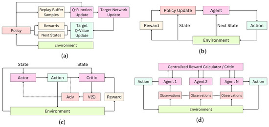
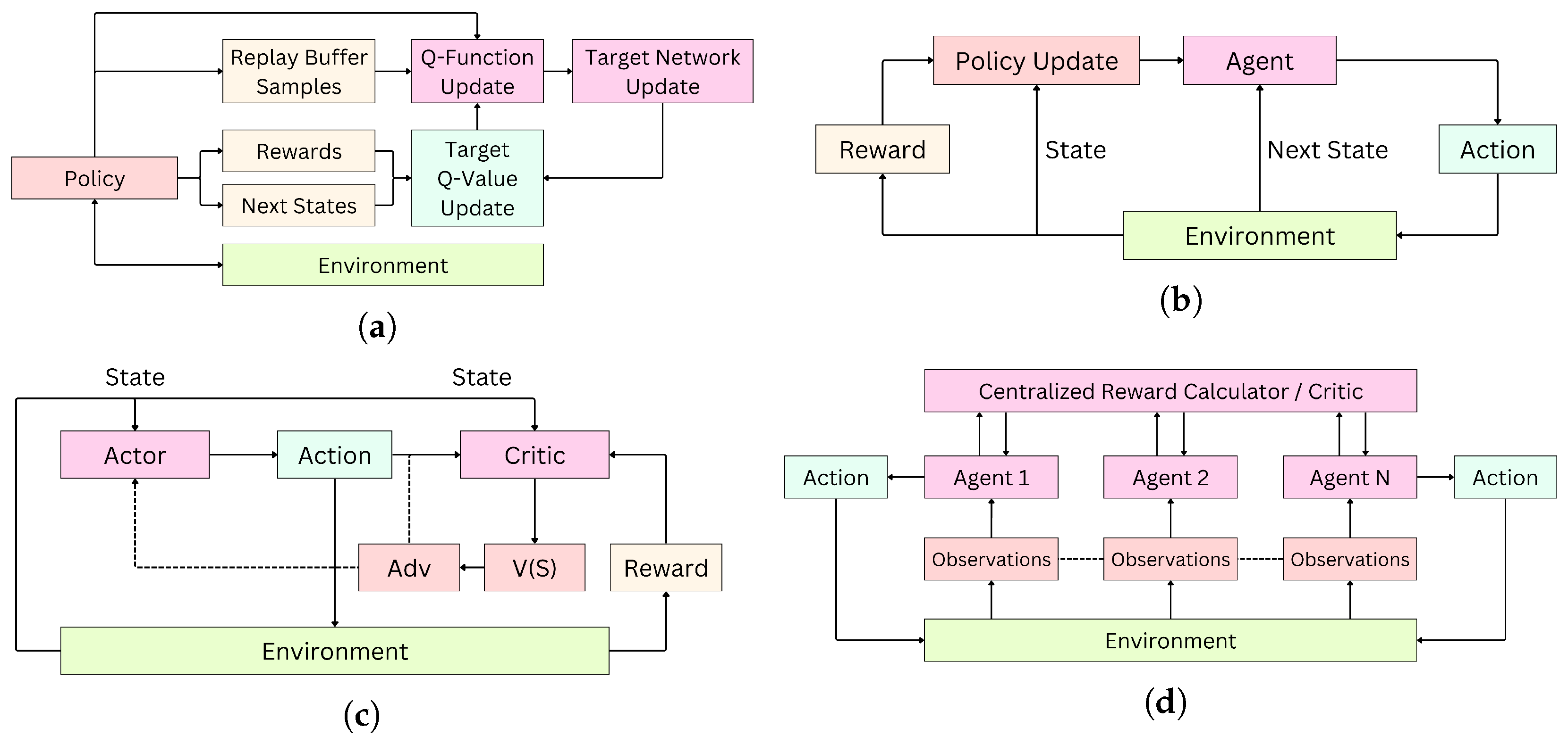
Value-based methods in RL are a class of algorithms that learn to make decisions by estimating the value of different states or state–action pairs and then using these value estimates to derive an optimal policy (see Figure 2a). Q-Learning is a value-based, model-free RL algorithm that learns an action-value function (Q-function) to estimate the expected cumulative reward for each action in a given state. DQN [39], on the other hand, uses neural networks to approximate the Q-function, enabling scalability to high-dimensional state spaces. Key algorithms in this spectrum also include Double DQN [40], Dueling DQN [41], and Prioritized Experience Replay. These approaches improve learning stability and sample efficiency but are primarily limited to discrete action spaces, making them less suitable for UAVs with continuous control requirements.

Figure 2. Block diagrams illustrating the core architecture and decision-making workflow of four major reinforcement learning paradigms: (a) value-based methods, which learn state-action values for policy derivation; (b) policy gradient methods, which directly optimize the policy through gradient ascent; (c) actor–critic methods, combining value estimation (critic) with policy optimization (actor); and (d) multi-agent RL (MARL), which enables cooperative or competitive behavior through multiple interacting agents.

2.3.2. Policy Gradient Methods

Policy gradient (PG) methods directly optimize the policy (a mapping from states to actions) by estimating gradients of expected return with respect to policy parameters (see Figure 2b). They are well suited for continuous or high-dimensional action spaces, where Q-value methods often struggle. These methods include REINFORCE, Trust Region Policy Optimization (TRPO) [42], and Proximal Policy Optimization (PPO) [43]. They have demonstrated superior performance in continuous action spaces, making them more applicable to UAV navigation.

2.3.3. Actor–Critic Methods

The actor–critic (AC) methods combine value-based and policy-based approaches by maintaining two models: the actor (policy) and the critic (value function) (see Figure 2c). This hybrid design benefits from stable value estimates while optimizing flexible policies. This involves the use of A3C (Asynchronous Advantage Actor–Critic), DDPG (Deep Deterministic Policy Gradient) [44], SAC (Soft Actor–Critic) [45], and TD3 (Twin Delayed DDPG). These algorithms are widely used for trajectory optimization, building upon the advantages attributed to off-policy learning and entropy regularization.

2.3.4. Multi-Agent RL (MARL)

MARL extends traditional RL to scenarios involving multiple agents interacting within a shared environment, using cooperative along with competitive learning paradigms [46]. These agents may be cooperative, competitive, or mixed, and the learning dynamics become significantly more complex due to the non-stationarity introduced by simultaneously learning agents (see Figure 2d). Common paradigms include Centralized Training with Decentralized Execution (CTDE), Independent Q-Learning (IQL), Multi-Agent DDPG (MADDPG) [47], Multi-Agent PPO (MAPPO), QMIX, and Value Decomposition Networks (VDNs). MADDPG has been successfully applied to UAV swarm coordination, showing improved adaptability and robustness compared to traditional rule-based methods [48,49]. Other MARL algorithms, such as QMIX [50] and COMA (Counterfactual Multi-Agent Policy Gradients) [51], are also used for UAV cooperation tasks, focusing on credit assignment and cooperative learning. These approaches demonstrate potential for decentralized control in UAV formations, but require extensive training and are computationally intensive.

Considerable attention has also been given to the simulation-to-real (sim2real) gap in RL-based UAV systems [52], prompting research into domain randomization and transfer learning techniques. Additionally, hierarchical RL has emerged as a valuable strategy for long-horizon UAV tasks, enabling high-level goal planning combined with low-level control policies [53]. Reward shaping remains a critical challenge in UAV path planning, with improper design leading to suboptimal or unstable behavior; several recent works have introduced curriculum learning and reward decomposition frameworks to address this issue [54]. Real-time constraints and computational efficiency are becoming central themes in RL-based UAV navigation. Researchers are exploring lightweight neural architectures [55] and model-based RL techniques [56] to reduce training times and improve convergence speed. There is also a growing body of work that evaluates the robustness of RL policies under sensor noise and adversarial disturbances [57], underscoring the need for safe and reliable deployment in real-world applications.

2.4. Literature Gaps

Most existing work on UAV path planning either focuses on single-agent scenarios or assumes simplified dynamics in multi-agent setups. Some notable efforts, such as those by Luo et al. [48], have evaluated multi-agent RL techniques. Although promising, these approaches often rely on abstract simulations with limited consideration of real-world UAV dynamics or scalability to larger swarms. Furthermore, the performance metrics in previous studies frequently include the time to target, reward optimization, and collision rate but often lack detailed information on scalability and adaptability across various environments, the number of agents, and different algorithms. Moreover, while RL-based path planning has been extensively studied in 2D environments, transitioning to 3D scenarios introduces additional challenges, including altitude control and complex aerodynamics. Traditional 2D approaches often fail to generalize effectively in 3D spaces due to the increased complexity of state-action spaces and higher-dimensional decision making. Some recent studies have incorporated physics-based UAV simulations using AirSim [37] and Gazebo [58] to model realistic flight dynamics. These high-fidelity simulations enable RL algorithms to learn policies that generalize better to real-world conditions.

Our work builds on this foundation by addressing critical gaps in the literature. We systematically compare multiple cutting-edge RL algorithms in both 2D and 3D environments. Unlike previous studies using simplified 2D environments, we incorporate a physics-based 3D simulator to model realistic UAV dynamics, including turn rates and checkpoint navigation. Our evaluation introduces comprehensive metrics, including collision probability per section, average reward, average time to complete all checkpoints, distance to final goal, and total distance covered, providing a holistic view of each algorithm’s performance. By transitioning from a Python-based 2D environment to a physics-based 3D setup, we highlight the challenges and tradeoffs in adapting RL algorithms to more complex and realistic scenarios. This helps researchers understand the suitability and limitations of RL algorithms for UAV swarm navigation, thereby bridging the gap between theoretical research and real-world applicability.

3. Problem Formulation

3.1. Path Planning Based on RL

The problem of path planning in UAV swarms can be effectively formulated as a reinforcement learning (RL) problem, where each UAV acts as an autonomous agent navigating itself in a dynamic environment with obstacles. The RL framework includes the following components discussed below.

3.1.1. States Space

The state $s_t$ (at time t) represents the current environment status as perceived by the UAV. For a UAV i, the state $s_t^i$ is defined as

$$s_t^i=\{p_t^i,v_t^i,d_t^i,o_t^i\}$$

(1)

where $p_t^i\in {\mathbb{R}}^n$ is the UAV’s position in n-dimensional space (2D or 3D), $v_t^i\in {\mathbb{R}}^n$ is the velocity vector, $d_t^i$ represents the distance to the target, and $o_t^i$ encodes obstacle proximity information, such as distances to nearby obstacles and other agents in the swarm. The joint state for an N UAV swarm is defined as

$$S_t=\{s_t^1,s_t^2,\dots ,s_t^N\}$$

(2)

3.1.2. Actions Space

The action $a_t^i$ for UAV i specifies its movement decision at time t. In a 2D environment, $a_t^i$ could correspond to changes in direction or velocity, which are defined as follows:

$$a_t^i=\{\Delta {\theta }_t^i,\Delta v_t^i\}$$

(3)

where $\Delta {\theta }_t^i$ is the change in heading direction, and $\Delta v_t^i$ is the change in velocity. For 3D environments, an additional dimension for altitude adjustment $\Delta h_t^i$ is included:

$$a_t^i=\{\Delta {\theta }_t^i,\Delta v_t^i,\Delta h_t^i\}$$

(4)

Depending on the RL algorithm used, the action spaces can either be discrete (predefined movement directions) or continuous (smooth velocity changes).

3.1.3. Reward Function

The reward function $R_t^i$ guides the behavior of the UAV toward achieving the final goal as efficiently as possible while avoiding collisions. For each UAV i, the reward (at time t) is defined as

$$R_t^i=r_{\mathrm{target}}^i-r_{\mathrm{collision}}^i-r_{\mathrm{effort}}^i$$

(5)

where $r_{\mathrm{target}}^i$ is a positive reward for reducing the distance to the target, proportional to $\parallel p_t^i-p_{\mathrm{target}}^i\parallel$, $r_{\mathrm{collision}}^i$ is a penalty for collisions with obstacles or other UAVs, and $r_{\mathrm{effort}}^i$ penalizes unnecessary energy expenditure, like excessive velocity or direction changes. The cumulative reward for a UAV i during an episode is given by

$$G_t^i=\sum _{t^{\prime }=t}^T{\gamma }^{t^{\prime }-t}{R}_{t^{\prime }}^i$$

(6)

where T is the duration of an episode, and $\gamma \in [0,1]$ is the discount factor.

3.1.4. Policy and Objective

The primary objective of an RL agent is to learn a particular policy $\pi \left(a_t^i\right|s_t^i)$ that optimizes the total anticipated reward.

$$J\left(\pi \right)={\mathbb{E}}_{\pi }\left[\sum _{t=0}^T{\gamma }^t{R}_t^i\right]$$

(7)

The policy $\pi$ can be represented by neural networks in deep RL methods, enabling the UAV to generalize to complex environments. Algorithms like SAC and PPO optimize the objective using policy gradients and entropy regularization to encourage exploration.

3.2. Multi-Agent Extension

In case of a multi-UAV swarm, the RL problem extends to multi-agent settings. Each UAV i optimizes its policy ${\pi }^i\left(a_t^i\right|s_t^i)$ while considering interactions with other UAVs. Coordination is achieved through decentralized policies, where each agent independently learns to avoid collisions and achieve its objective or through centralized training with shared reward structures.

Path planning for multi-agent UAV swarms introduces additional complexities beyond single-agent scenarios due to swarm dynamics, coordination, and collision avoidance. Each UAV operates within a shared environment, necessitating strategies that enable efficient goal achievement while maintaining safety and cooperation among agents. This subsection elaborates on the multi-agent extensions of the RL framework, incorporating mathematical formulations for swarm behavior and interactions.

3.2.1. Joint State and Action Spaces

In a multi-agent system comprising N UAVs, the joint state (at time t) is defined as $S_t=\{s_t^1,s_t^2,\dots ,s_t^N\}$, where $s_t^i$ depicts the state of i-th UAV, as defined in a single-agent setting. Similarly, the joint action space is $A_t=\{a_t^1,a_t^2,\dots ,a_t^N\}$, where $a_t^i$ denotes UAV action i at time t. The dimensionality, along with the complexity of the action space, increases with the number of agents, making the path planning problem inherently more challenging.

3.2.2. Inter-Agent Dependencies

In practical multi-agent scenarios, UAVs may not access global state $S_t$ but instead rely on partial observations. For UAV i, the observation $o_t^i$ is a subset of $S_t$ containing $o_t^i=\{s_t^i,\mathrm{relative}\mathrm{velocities}\mathrm{and}\mathrm{positions}\mathrm{of}\mathrm{nearby}\mathrm{agents}\}$. The neighborhood of UAV i is defined using a sensing radius r, and the inter-agent dependencies are modeled as

$${\mathcal{N}}_t^i=\{j\mid \parallel p_t^i-p_t^j\parallel \le r,j\ne i\}$$

(8)

where ${\mathcal{N}}_t^i$ represents the set of agents within r of UAV i.

3.2.3. Reward Sharing and Conflict Resolution

Multi-agent path planning introduces conflicts between agents, like competing trajectories or shared resource constraints. To address this, reward functions are designed to include inter-agent considerations like $R_t^i=r_{\mathrm{individual}}^i+r_{\mathrm{coordination}}^i$, where $r_{\mathrm{individual}}^i$ encourages UAV i to achieve its specific target while avoiding collisions, and $r_{\mathrm{coordination}}^i$ incentivizes behaviors that benefit the swarm, such as preventing congestion. A coordination mechanism based on priority scheduling is implemented to resolve conflicts dynamically.

3.2.4. Swarm Dynamics

Swarm behavior emerges from the close coordination of individual agents following decentralized policies. To ensure coordinated motion, consensus dynamics are introduced:

$$p_{t+1}^i=p_t^i+\Delta t\left[\alpha (p_{\mathrm{target}}^i-p_t^i)+\beta \sum _{j\in {\mathcal{N}}_t^i}(p_t^j-p_t^i)\right]$$

(9)

where $\alpha$ and $\beta$ are weights controlling the influence of target attraction and inter-agent alignment, respectively, and $\Delta t$ is the time step. This formulation strikes a balance between individual goal achievement and swarm cohesion.

3.2.5. Collision Avoidance

Collision avoidance is crucial in multi-agent systems, necessitating real-time adjustments to dynamic environments. For UAV i, the collision avoidance constraint ensures $\parallel p_t^i-p_t^j\parallel \ge d_{\min },\forall j\ne i$, where $d_{\min }$ is the minimum safe distance between UAVs. To incorporate this constraint into the RL framework, the reward function is equipped with a penalty for violating $d_{\min }$:

$$r_{\mathrm{collision}}^i=-\lambda \sum _{j\in {\mathcal{N}}_t^i}max(0,d_{\min }-\parallel p_t^i-p_t^j\parallel )$$

(10)

where $\lambda >0$ is the penalty weight.

3.2.6. Training Paradigms

Multi-agent RL can follow two paradigms, out of which the first one is Decentralized Training and Execution (DTE), where each UAV trains an independent policy ${\pi }^i\left(a_t^i\right|o_t^i)$, relying solely on local observations and rewards. The second training paradigm is Centralized Training with Decentralized Execution (CTDE), where a centralized critic evaluates the global state ($S_t$) along with joint actions ($A_t$) during training. At the same time, the policies ${\pi }^i$ remain decentralized during execution. CTDE is particularly effective in addressing non-stationarity and coordination challenges, as it enables agents to learn from global information without requiring centralized control during deployment. The scalability of multi-agent RL methods to large swarms is a critical consideration. Our approach utilizes shared policy architectures to enhance generalization across varying swarm sizes and environmental complexities.

The transition from 2D to 3D modeling significantly alters the problem formulation for UAV path planning, introducing additional complexities and considerations. In 2D modeling, the state of a UAV is defined in a planar coordinate system $s_t^{2\mathrm{D}}=\{x_t,y_t,{\theta }_t,v_t\}$, where $(x_t,y_t)$ represents the UAV’s position, ${\theta }_t$ is its orientation, and $v_t$ is its velocity. In contrast, 3D modeling introduces an additional degree of freedom, expanding the state to $s_t^{3\mathrm{D}}=\{x_t,y_t,z_t,{\varphi }_t,{\psi }_t,{\theta }_t,v_t\}$, where $z_t$ denotes altitude, and ${\varphi }_t$ and ${\psi }_t$ represent the pitch and yaw angles, respectively. This richer state space increases the problem’s dimensionality and the complexity of the policy search.

In 2D environments, actions are typically defined as changes in velocity or heading $a_t^{2\mathrm{D}}=\{\Delta v,\Delta \theta \}$. For 3D environments, the action space expands to include changes in altitude and additional rotational controls $a_t^{3\mathrm{D}}=\{\Delta v,\Delta \theta ,\Delta z,\Delta \varphi ,\Delta \psi \}$. This expanded action space requires algorithms to learn more complex control policies, as UAVs must navigate three-dimensional obstacles while maintaining stability and adhering to dynamic constraints. In 2D, obstacles and targets are confined to a planar space, allowing for simplified collision detection and path planning. UAVs are modeled as points, and 2D geometric constraints govern the dynamics of the environment. On the other hand, in 3D, obstacles occupy volumetric space. Collision avoidance requires accounting for spatial relationships in all three dimensions, and path planning must optimize routes that navigate through both horizontal and vertical constraints—the dimensional change from 2D to 3D increases the computational complexity of simulation and policy training. In 3D, the search space for optimal policies is significantly larger, requiring more sophisticated exploration strategies and substantial computational resources. Additionally, 3D modeling often involves the use of physics engines for realistic simulation, which introduces higher fidelity but also more significant computational overhead. The shift to 3D modeling more accurately approximates real-world UAV operations, providing more realistic evaluations of RL algorithms. However, advanced techniques are required to manage increased complexity. Our study evaluates RL algorithms across 2D and 3D setups, highlighting their adaptability and performance in these differing contexts.

4. Experiments and Simulation Environments

We trained and tested 5 different reinforcement learning algorithms, namely, SAC, PPO, DDPG, TRPO, and MADDPG, using the same training setup for a scenario involving multiple autonomous UAVs navigating through unknown environments with obstacles. The goal of every UAV is to reach its respective destination in as little time and as few steps as possible. Hyperparameters used for all five algorithms are detailed in Table 2.

Table 2. Hyperparameters used for SAC, PPO, DDPG, TRPO, and MADDPG algorithms.

Hyperparameter	SAC	PPO	DDPG	TRPO	MADDPG
Buffer Size	20,480	-	100,000	-	1,000,000
Batch Size	2048	2048	256	5000	1024
Learning Rate	$3.0\times {10}^{-4}$	$2.5\times {10}^{-4}$	$1.0\times {10}^{-4}$	$1.0\times {10}^{-3}$	$1.0\times {10}^{-3}$
Entropy Coefficient ($\beta$)	$1.0\times {10}^{-2}$	$5.0\times {10}^{-2}$	-	$1.0\times {10}^{-4}$	$1.0\times {10}^{-2}$
Discount Factor ($\gamma$)	0.99	0.99	0.99	0.99	0.95
Clip Range ($ϵ$)	-	0.2	-	0.01	-
GAE ($\lambda$)	-	0.95	-	0.97	-
Target Network Update Rate ($\tau$)	0.005	-	0.005	-	0.01
Noise Standard Deviation	-	-	0.2	-	0.2

4.1. Training Environments

Two types of environments were used to evaluate all five algorithms: a two-dimensional Python environment representing agents as points in space and a three-dimensional Unity environment containing fixed-wing UAVs incorporating realistic physics.

4.1.1. Two-Dimensional Python Environment (P2D)

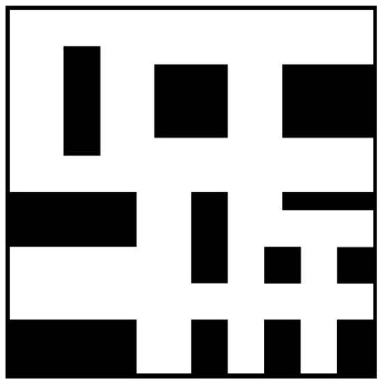
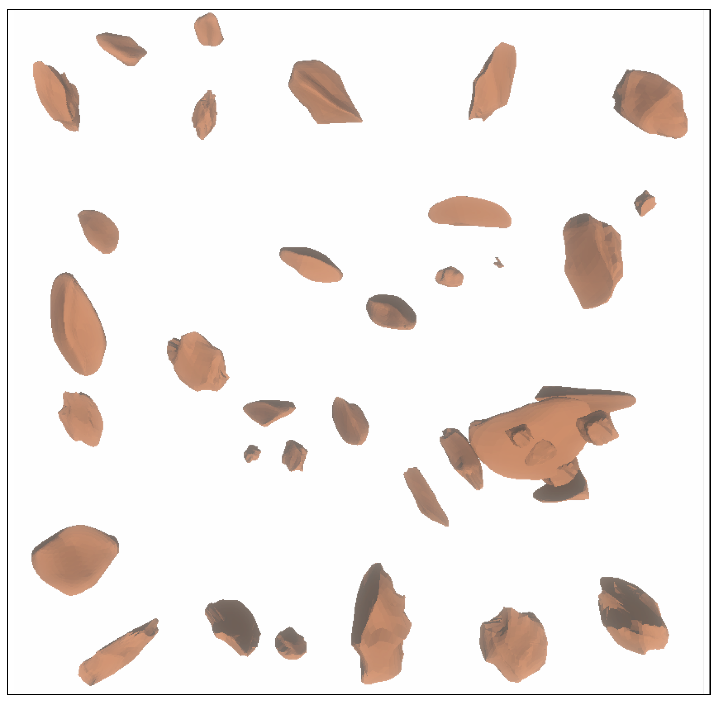
P2D provides a simplified yet dynamic simulation framework for training RL agents to perform autonomous multi-agent UAV path planning in a 2D space having obstacles (as depicted in Figure 3). The objective is to enable UAVs to navigate from their initial positions to designated targets in the shortest time possible and with efficient resource utilization while avoiding collisions with other agents and static obstacles. The environment is implemented as a modular Python-based simulation with the following components:

Figure 3. Base map in two-dimensional Python environment (P2D).

• main.py: Manages the training loop, hyperparameters, and simulation control.
• environment.py: Defines the environment class and the reward mechanism, including observation and action spaces.
• buffer_class.py: Implements experience replay for training RL agents.
• agent_functions.py: Constructs the actor and critic networks and the policy function.

The observation space is represented as a 2D grid of size $75\times 75$ centered around the UAV’s current position. Each cell value $o_{ij}\in [-1,1]$ depicts the normalized distance to the nearest obstacle within the UAV’s field of view. The grid captures the local environment, allowing the UAV to make informed navigation decisions. $\mathcal{O}=\{o_{ij}\mid i,j\in [1,\mathrm{observation}\_\mathrm{size}]\}$, where $\mathrm{observation}\_\mathrm{size}=75$. Action space for each UAV is continuous and represented by the angle $\theta \in [\min \_\mathrm{angle},\max \_\mathrm{angle}]$ in radians, specifying the UAV’s turn direction. The angular range is discretized for computational efficiency, with the minimum and maximum angles defined as $\min \_\mathrm{angle}=0^{\circ },\max \_\mathrm{angle}=359.{99}^{\circ }.$ Key components of the reward function in this case are

$$r_t=r_{\mathrm{obstacle}}+r_{\mathrm{goal}}+r_{\mathrm{time}}+r_{\mathrm{potential}}+r_{\mathrm{angle}}$$

(11)

where

$r_{\mathrm{obstacle}}=-10$ if the UAV collides with an obstacle;

$r_{\mathrm{goal}}=+20$ if the UAV reaches its target;

$r_{\mathrm{time}}=-0.2$ penalty per time step;

$r_{\mathrm{potential}}=\Delta$ potential change in distance to nearest obstacle;

$r_{\mathrm{angle}}=-|\Delta \theta |$ penalty for excessive angle changes.

Each UAV has a maximum speed of $0.14$ units per step and maintains a safe distance of $2.5$ units from other UAVs and $1.2$ units from static obstacles. While all UAVs operate independently with decentralized policies, the shared environment and observation setup inherently introduce an implicit form of cooperative behavior. Each UAV is aware of the positions of other agents through its observation space and learns to treat them as dynamic obstacles, adjusting its trajectory to maintain safe distances and avoid collisions. This results in emergent coordination patterns, where agents dynamically adapt their paths in relation to others. The UAVs operate within a field of view of $180$, with an angular resolution of $0.9°$. Moreover, they rely on their local observation grid and individual reward structure to make actions, emulating a decentralized navigation strategy.

Hyperparameter values for P2D are selected based on a combination of empirical studies and practical considerations specific to path planning in continuous action spaces. A lower actor learning rate $\left(0.0001\right)$ is preferred for smoother policy updates, while a slightly higher critic learning rate $\left(0.001\right)$ helps stabilize value estimation. Discount factor $\left(\gamma \right)=0.95$ provides a balance between short-term reactivity and long-term goal optimization. Batch size and episode length are empirically selected after preliminary experiments for stable convergence. The exploration noise standard deviation ($0.3$) is set to encourage sufficient policy exploration during early training while remaining within safe bounds of maneuverability.

P2D environment provides a lightweight platform for evaluating RL algorithms for multi-agent path planning. The grid-based observation space and reward structure facilitate rapid prototyping and comparative analysis, laying the groundwork for transitioning to more complex, physics-based 3D simulations.

4.1.2. Three-Dimensional Unity Environment (U3D)

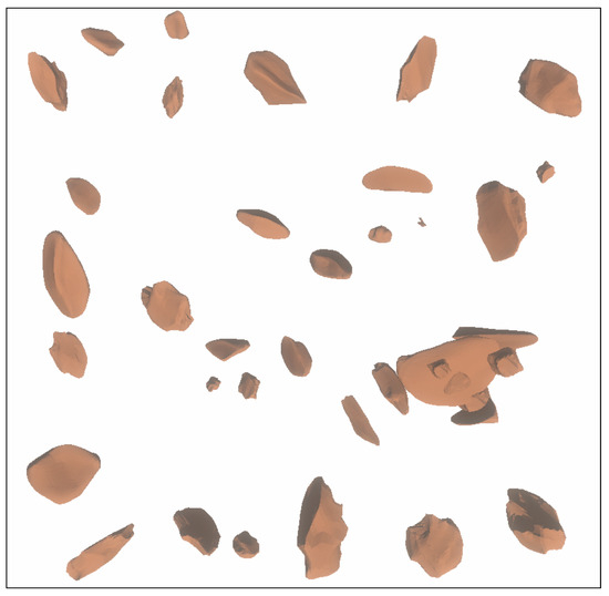
This setup is for training autonomous fixed-wing UAVs in 3D environments (as seen in Figure 4). The main objective of UAVs in this case is to reach their final target while passing through a series of checkpoints (intermediate targets) in as little time as possible while avoiding collisions with fixed obstacles and other UAVs. The environment is simulated using Unity 3D, and the training setup is based on the ML-Agents framework. The observation space for each UAV consists of multiple components to capture its state within the 3D environment. The key features of the observation space are the following:

Figure 4. Base map in three-dimensional Unity environment (U3D) [59].

• Velocity of the UAV in the 3D space is represented by a 3-dimensional vector $\mathbf{v}=[v_x,v_y,v_z]$, where $v_x$, $v_y$, and $v_z$ represent the velocity components along x, y, and z axes, respectively.
• The relative distance to the next checkpoint is represented by the vector $\mathbf{d}=[d_x,d_y,d_z]$, where $d_x$, $d_y$, and $d_z$ represent the relative position of the UAV relative to the next checkpoint in the 3D space.
• Orientation of the UAV concerning the next checkpoint is represented by a 3-dimensional vector $\mathbf{o}=[o_x,o_y,o_z]$, where $o_x$, $o_y$, and $o_z$ describe the directional vector pointing towards the next checkpoint.
• Environment includes 15 perception rays cast from the front of the UAV. Each ray provides information about the distance to the nearest obstacle in its path. Each ray provides a vector ${\mathbf{r}}_{\mathbf{i}}=[r_{ix},r_{iy},r_{iz}]$, where $i\in \{1,2,\dots ,15\}$ represents the index of the ray, and $r_{ix}$, $r_{iy}$, and $r_{iz}$ are the components of the distance vector. The rays are cast to a maximum distance of 250 units in front of the UAV and are limited to a 70-degree field of view.

Observation space’s total size is computed as $\mathrm{Total}\mathrm{Observation}\mathrm{Space}=\left(3\mathrm{for}\mathrm{velocity}\right)+\left(3\mathrm{for}\mathrm{relative}\mathrm{distance}\right)+\left(3\mathrm{for}\mathrm{orientation}\right)+(15\times 3\mathrm{for}\mathrm{perception}\mathrm{rays})=3+3+3+45=54\mathrm{dimensions}.$ Action space consists of controls that modify the orientation and movement of the UAV within the 3D environment. Specifically, the UAV has control over its pitch and yaw. Yaw control refers to the rotation of the UAV around the z axis. The directional commands for yaw can be as follows: turning left (−1), maintaining the current orientation (0), or turning right (+1). Pitch control refers to the rotation of the UAV around the y axis. Similarly, the directional commands for pitch can be as follows: pitching down (−1), maintaining the current pitch (0), or pitching up (+1). Upon receiving a yaw and pitch command, the UAV applies forward thrust and adjusts its rotation accordingly, with corresponding actions in the 3D environment. Here, although the agent issues high-level directional commands, the actual execution of these commands in the U3D physics environment results in continuous actions. A command to turn left is translated into a gradual change in orientation through the UAV’s rigid body dynamics, respecting the constraints of angular velocity and inertia. The following parameters govern the UAV’s movement:

• Forward thrust is controlled by a value of 100,000 units. This value controls the UAV’s speed and propulsion.
• UAV’s maximum angular velocity for pitch, yaw, and roll is capped at 100 degrees per second.
• Roll angle is adjusted between −180 and +180 degrees based on yaw and pitch commands.
• Maximum pitch and yaw angles are constrained to be between −45 and +45 degrees.

If the UAV collides with an obstacle, it incurs a penalty proportional to the inverse of the distance to the obstacle. This is modeled as $r_{\mathrm{obstacle}}=-{\displaystyle \frac{1}{\mathrm{distance}\mathrm{to}\mathrm{obstacle}}}$ for collision or −1 for direct hit. When a UAV reaches a checkpoint, it earns a reward of +0.5. A time penalty is applied after every step to encourage the agent to minimize its steps. This is given by $r_{\mathrm{time}}=-{\displaystyle \frac{1}{\mathrm{MaxSteps}}}\mathrm{per}\mathrm{step}.$ If the UAV takes too long (i.e., the step count exceeds the next checkpoint timeout), an additional penalty of −0.5 is applied. In total, 54 dimensions represent the environment’s total observation space, and the action space is formed by the yaw and pitch directional commands as described earlier.

4.1.3. Simulation Setup and Parameters

For consistency and reproducibility of experiments, we provide a summary of the simulation setup and parameters used throughout this study. Table 3 presents the key settings for path planning tasks in both the P2D and U3D environments. These include observation space, action space, physics engine, and the hardware/software stack employed. The experiments were implemented using Python frameworks with compatible environments for both 2D and 3D simulations.

Table 3. Summary of simulation setup and parameters.

Parameter	Description
Observation Space	Relative Positions Obstacle Proximities Velocities
Action Space	Continuous (Thrust Vectoring)
Physics Engine	Custom Lightweight Kinematic Simulator
Software Used	Python 3.10—(P2D) Unity (ML-Agents) 3.8.0—(U3D)
Hardware Used	Intel Core i7, 32 GB RAM, NVIDIA RTX 3060 GPU—(P2D) Intel Core i7, 32 GB RAM, NVIDIA RTX 3080 GPU—(U3D)
Operating System	Ubuntu 22.04 LTS—(P2D) Windows 10—(U3D)

Multiple metrics were extracted to compare all five RL algorithms across the two environments. The definitions and methods to compute these metrics are presented in the following sections.

4.2. Obstacle-Hitting Probability

In UAV swarming, the “obstacle-hitting probability” statistic calculates the chance that UAVs may collide with obstacles. A more negligible probability denotes improved navigation, safety, and obstacle awareness, whereas a greater probability suggests inadequate path planning, insufficient collision avoidance, or inefficient algorithms. It is essential for assessing swarm dependability in intricate settings.

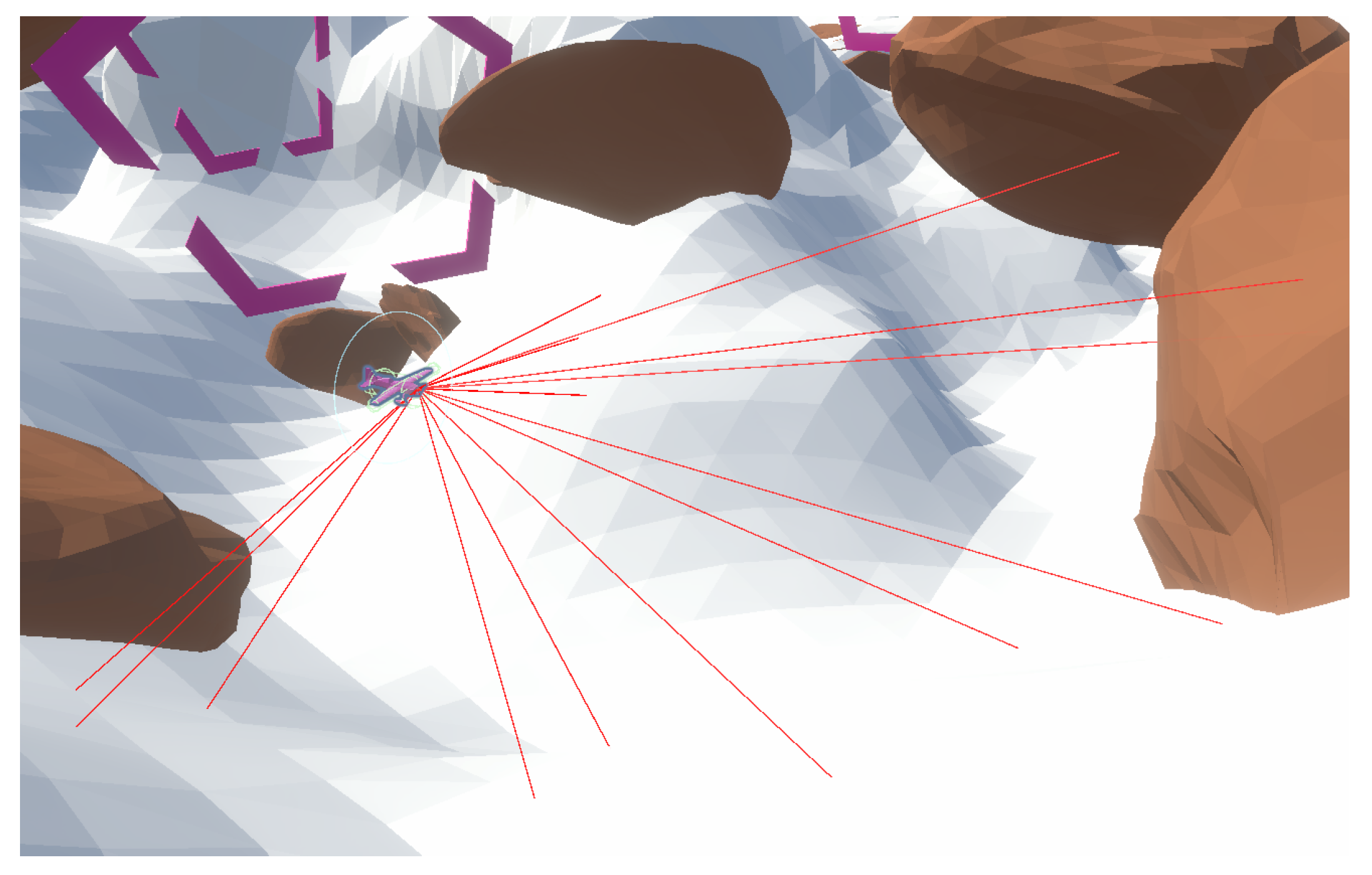
The obstacle-hitting probability is calculated using observations (distance) returned from raycasting. In this case, a ray is the part of the line that starts from the tip of the UAV/agent and goes off in a particular direction. Raycasting is the process of sending invisible rays, similar to lidar rays, out in a specific direction and watching to see if they strike anything. Assume that we create a ray from point O to point P, if an object interrupts this ray, the distance of that object can be easily extracted. To cast rays in a Unity3D environment, we used the static method Physics.Raycast( ), which belongs to the Physics class. We can either explicitly provide parameters like the start location, direction, and magnitude of the ray that will be cast, or we can generate a ray in advance and utilize it as a parameter for the procedure.

In this case, we cast 15 rays in total (see Figure 5). In total, five rays were cast in the same plane: five in the upwards direction and five in the downwards direction. The viewing angle of these rays was from −70 degrees to +70 degrees with respect to the centerline drawn straight outwards from the tip of the UAV. All 15 rays’ intensity values were adjusted according to the distance/proximity value they are returning.

Figure 5. All 15 rays cast out of the agent, returning proximity values in the entire frontal field.

The obstacle-hitting probability (OHP) quantifies the likelihood of UAVs colliding with obstacles while navigating through our environment. This probability is computed using raycast distances to obstacles averaged over time and space within the environment. Let $n_r=15$ represent a total number of rays cast by the UAV. At any time step t, the distances recorded by the $i-th$ ray are denoted by $d_i\left(t\right)$, where $i=1,2,\dots ,n_r$. The proximity $p_i\left(t\right)$ for the $i-th$ ray at time t is computed as the inverse of the distance.

$$p_i\left(t\right)=\left\{\begin{array}{cc}{\displaystyle \frac{1}{d_i\left(t\right)}},\hfill & \mathrm{if}{d}_i\left(t\right)>0,\hfill \\ 0,\hfill & \mathrm{if}{d}_i\left(t\right)=0(\mathrm{no}\mathrm{obstacle}\mathrm{detected})\hfill \end{array}\right.$$

(12)

Average proximity across all rays at a single time step t is

$$P\left(t\right)={\displaystyle \frac{1}{n_r}}\sum _{i=1}^{n_r}{p}_i\left(t\right)$$

(13)

For a segment between two checkpoints (e.g., $t_1$ to $t_2$), the segment-level OHP is calculated by averaging the proximities over all steps in the segment.

$$OH{P}_{\mathrm{segment}}={\displaystyle \frac{1}{t_2-t_1+1}}\sum _{t=t_1}^{t_2}P\left(t\right)$$

(14)

Our entire course was divided into $m\left(15\right)$ segments (between multiple checkpoints), and the overall course-level OHP was calculated as the average of all segment-level OHPs.

$$OH{P}_{\mathrm{course}}={\displaystyle \frac{1}{m}}\sum _{j=1}^{m}OH{P}_{\mathrm{segment},j}$$

(15)

4.3. Distance to Goal

In UAV swarming, the “distance to goal” statistic shows algorithm performance, mission success, and navigation efficiency. A shorter distance indicates the best possible path planning, whereas a longer distance indicates inefficiencies or avoiding obstacles. It is a crucial component in assessing the efficacy of UAV swarms, as it affects energy consumption and reflects the flexibility in changing conditions.

Let n denote the total UAVs in the environment. The state of the i-th UAV (at any time t) can be depicted by its position in a 2D space as $p_i\left(t\right)=(x_i\left(t\right),y_i\left(t\right))$. Similarly, target location for the i-th UAV is given by $g_i=(x_{g,i},y_{g,i})$. The Euclidean distance between the UAV’s position $p_i\left(t\right)$ and its target $g_i$ is given by

$$d_i\left(t\right)=\sqrt{{(x_i\left(t\right)-x_{g,i})}^2+{(y_i\left(t\right)-y_{g,i})}^2}$$

(16)

At the end of an episode (denoted by T), the final distance to the goal for the i-th UAV is

$$d_i\left(T\right)=\sqrt{{(x_i\left(T\right)-x_{g,i})}^2+{(y_i\left(T\right)-y_{g,i})}^2}$$

(17)

For n UAVs, the individual distances to the goal at the end of the episode are $d_1\left(T\right),d_2\left(T\right),\dots ,d_n\left(T\right)$. The average distance to the goal across all UAVs is computed as $\mathrm{Distance}\mathrm{to}\mathrm{Goal}={\displaystyle \frac{1}{n}}{\sum }_{i=1}^n{d}_i\left(T\right)$. Substituting the expression for $d_i\left(T\right)$, the final average distance to the goal is

$$\mathrm{Distance}\mathrm{to}\mathrm{Goal}={\displaystyle \frac{1}{n}}\sum _{i=1}^n\sqrt{{(x_i\left(T\right)-x_{g,i})}^2+{(y_i\left(T\right)-y_{g,i})}^2}$$

(18)

For the calculation of the distance to goal metric, we assume that all UAVs complete the episode (whether by reaching their target or ending due to other conditions like timeout or collision). The positions $p_i\left(T\right)$ are the final states of the UAVs at the end of each episode.

4.4. Total Distance Covered

In UAV swarming, the “total distance covered” metric shows how far the UAVs have gone. While a larger distance implies less-than-ideal routes or substantial obstacle avoidance, a shorter distance indicates effective path planning and lower energy use.

Let n denote the total UAVs in the environment. The state of the i-th UAV (at any time t) can be depicted by its position in a 2D space as $p_i\left(t\right)=(x_i\left(t\right),y_i\left(t\right))$. The total duration of the episode for all UAVs is T, where T is a total number of time steps in an episode. The distance covered by the i-th UAV between two consecutive time steps t and $t+1$ is given by the Euclidean distance.

$$\Delta d_i\left(t\right)=\sqrt{{(x_i(t+1)-x_i\left(t\right))}^2+{(y_i(t+1)-y_i\left(t\right))}^2}$$

(19)

To calculate the total distance covered by the i-th UAV during the entire episode, sum up the distances $\Delta d_i\left(t\right)$ over all time steps:

$$D_i=\sum _{t=1}^{T-1}\Delta d_i\left(t\right)=\sum _{t=1}^{T-1}\sqrt{{(x_i(t+1)-x_i\left(t\right))}^2+{(y_i(t+1)-y_i\left(t\right))}^2}$$

(20)

For n UAVs, the total distances covered by each UAV are $D_1,D_2,\dots ,D_n$. The average total distance covered across all UAVs is given by $\mathrm{Total}\mathrm{Distance}\mathrm{Covered}={\displaystyle \frac{1}{n}}{\sum }_{i=1}^n{D}_i$. Substituting the expression for $D_i$, the final formulation becomes

$$\mathrm{Total}\mathrm{Distance}\mathrm{Covered}={\displaystyle \frac{1}{n}}\sum _{i=1}^n\sum _{t=1}^{T-1}\sqrt{{(x_i(t+1)-x_i\left(t\right))}^2+{(y_i(t+1)-y_i\left(t\right))}^2}.$$

(21)

The time series data $p_i\left(t\right)$ for each UAV are available for all time steps $t=1,2,\dots ,T$ and all UAVs remain operational throughout the episode (or the distance computation stops when the UAV reaches its goal or ends its episode through either a collision or time runout).

4.5. Average Velocity

The “average velocity” metric in UAV swarming indicates the overall speed of UAVs during a mission. Higher average velocity reflects faster navigation and efficiency, while lower velocity may indicate obstacles, frequent stops, or inefficient path planning.

Let n denote total UAVs in an environment. For each UAV, we calculate its average velocity as the ratio of the total distance covered by the UAV during the episode to the total time it took to complete its episode. The total distance covered by the i-th UAV during the episode is given by

$$D_i=\sum _{t=1}^{T_i-1}\sqrt{{(x_i(t+1)-x_i\left(t\right))}^2+{(y_i(t+1)-y_i\left(t\right))}^2}$$

(22)

where $T_i$ is a total number of time steps for the i-th UAV until the episode ends for that UAV. The average velocity for the i-th UAV is defined as the ratio of the total distance covered ($D_i$) to the total time ($T_i$) it took for the episode and is mathematically expressed as $v_i={\displaystyle \frac{D_i}{T_i}}$. For n UAVs, the individual average velocities are $v_1,v_2,\dots ,v_n$. The overall average velocity across all UAVs is given by $\mathrm{Average}\mathrm{Velocity}={\displaystyle \frac{1}{n}}{\sum }_{i=1}^n{v}_i$. Substituting the expression for $v_i$, we get $\mathrm{Average}\mathrm{Velocity}={\displaystyle \frac{1}{n}}{\sum }_{i=1}^n{\displaystyle \frac{D_i}{T_i}}$. Substituting $D_i$ into the equation, the final average velocity comes out to be

$$\mathrm{Average}\mathrm{Velocity}={\displaystyle \frac{1}{n}}\sum _{i=1}^n{\displaystyle \frac{{\sum }_{t=1}^{T_i-1}\sqrt{{(x_i(t+1)-x_i\left(t\right))}^2+{(y_i(t+1)-y_i\left(t\right))}^2}}{T_i}}$$

(23)

The time series data $p_i\left(t\right)$ are available for all UAVs, and the episode length $T_i$ is known for each UAV. A UAV’s episode ends due to one of the following reasons: (1) reaching its target, (2) colliding with an obstacle or another UAV, (3) episode timeout.

5. Results and Discussion

To assess how well reinforcement learning (RL) algorithms perform in autonomous UAV swarm navigation, we conducted experiments both in 2D and 3D simulated environments. The scenarios were designed to test the algorithms under varying levels of complexity. Each environment included multiple UAVs, targets, and obstacles, ensuring that different navigation challenges arise during an episode. The experiments were conducted with consistent initial conditions across all algorithms to ensure a fair comparison, and each algorithm was trained for 2 million episodes.

Qualitative and quantitative information is gathered in both scenarios to perform the comparison. The results are broadly divided into two sections, i.e., P2D for 2D map results and U3D for 3D map results.

5.1. P2D Map Results

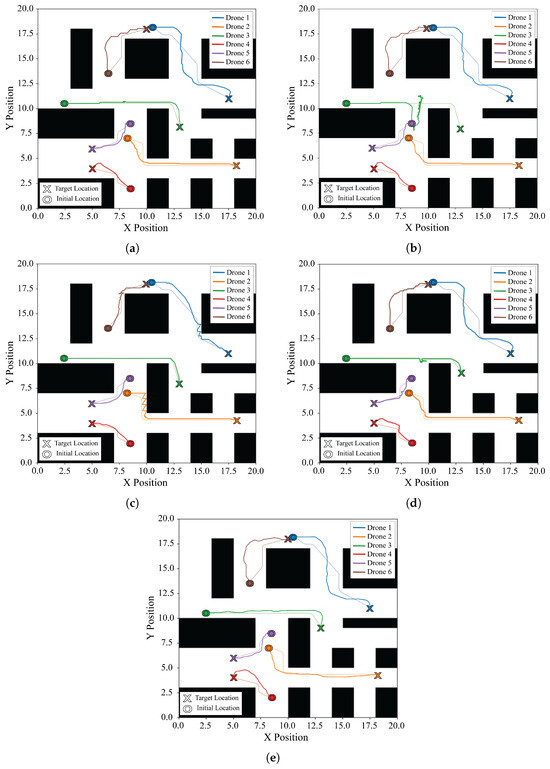
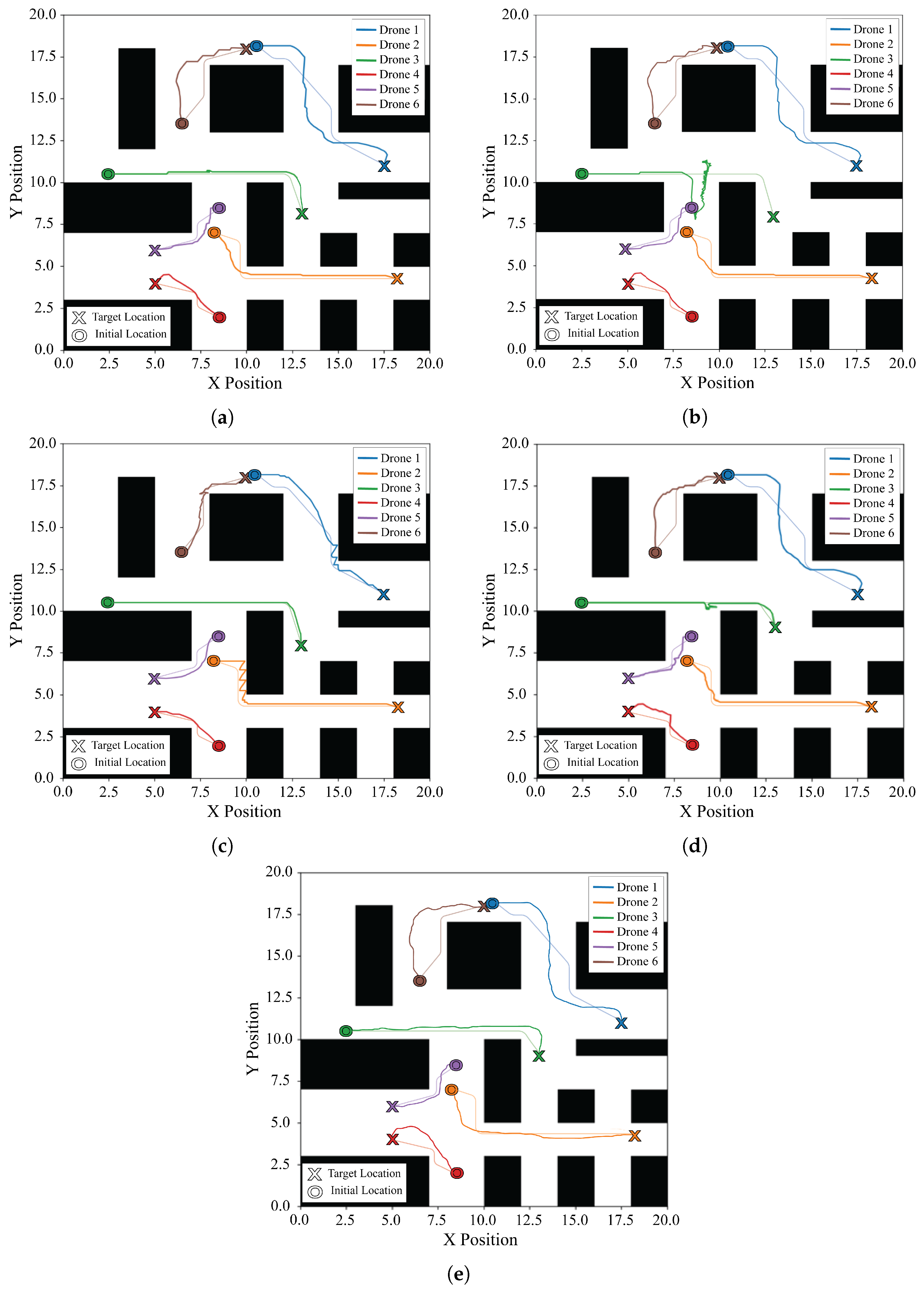
To compare UAV performances on 2D maps, qualitative information was gathered by analyzing screenshots and trajectories of the UAVs during navigation (as seen in Figure 6). DDPG exhibited smooth and efficient paths, successfully avoiding obstacles and optimizing the traversal between checkpoints. In contrast, SAC displayed slightly more exploratory behavior, resulting in occasional deviations from optimal paths, whereas PPO exhibited frequent abrupt policy changes, leading to a higher probability of obstacle hits. TRPO demonstrated stable and conservative policy updates, producing generally safe trajectories but with slightly longer path lengths due to its cautious step sizes. MADDPG, which benefited from centralized training with decentralized execution, demonstrated improved step efficiency in cooperative navigation. In dynamic environments (with moving obstacles or other agents), DDPG’s deterministic policy enables precise and adaptive actions, resulting in better navigation performance. SAC’s entropy-driven exploration is beneficial for discovering alternative paths, but it occasionally leads to unnecessary deviations. While ensuring stability, PPO’s clipped objective struggles with the fine-tuning required for complex and quick actions. TRPO remains robust in maintaining safe policies but at the expense of responsiveness, whereas MADDPG shows promising coordinated behavior, resulting in a slightly lower obstacle hitting probability than DDPG.

Figure 6. UAV trajectories for a six-agent swarm in P2D environment along with softly shaded reference A* trajectories. (a) DDPG (b) SAC (c) PPO (d) TRPO (e) MADDPG.

For analyzing results quantitatively, the comparison was performed on various metrics, including the average time to complete all checkpoints, the probability of hitting obstacles, and the cumulative reward achieved during training. The performance metrics for a 6-UAV swarm in P2D, along with respective standard deviations, are presented in Table 4, showcasing the average time to complete an episode, the average number of steps taken, and the average obstacle-hitting probability for each algorithm. The same metrics for a 10-UAV swarm and a 20-UAV swarm are presented in Table A3 and Table A4, respectively.

Table 4. Performance metrics across algorithms in two-dimensional Python environment for a 6-agent UAV swarm. For each UAV, time taken (in seconds) and steps taken are reported as mean ± standard deviation over 6 independent runs.

	UAV 1		UAV 2		UAV 3		Obstacle Hitting Probability
	Time (s)	Steps	Time (s)	Steps	Time (s)	Steps
SAC	107 (±3.1)	102 (±1.7)	096 (±2.2)	091 (±3.0)	154 (±5.3)	175 (±6.2)	∼16%
PPO	125 (±4.5)	129 (±3.8)	108 (±4.2)	113 (±3.9)	076 (±1.6)	081 (±1.9)	∼39%
TRPO	098 (±2.7)	101 (±1.6)	094 (±2.4)	087 (±1.9)	090 (±2.1)	093 (±2.2)	∼21%
DDPG	097 (±2.3)	096 (±1.5)	091 (±2.0)	089 (±1.7)	083 (±1.9)	075 (±1.6)	∼15%
MADDPG	092 (±2.1)	094 (±1.4)	085 (±1.9)	088 (±1.8)	075 (±1.7)	077 (±1.5)	∼14%
	UAV 4		UAV 5		UAV 6		Obstacle Hitting Probability
	Time (s)	Steps	Time (s)	Steps	Time (s)	Steps
SAC	069 (±1.2)	061 (±1.3)	067 (±1.1)	061 (±1.1)	083 (±2.2)	077 (±1.3)	∼16%
PPO	051 (±1.6)	054 (±1.4)	057 (±1.9)	059 (±1.1)	066 (±1.5)	066 (±2.0)	∼39%
TRPO	058 (±1.5)	060 (±1.2)	058 (±1.7)	060 (±1.3)	069 (±1.8)	072 (±1.6)	∼21%
DDPG	062 (±1.1)	057 (±1.6)	061 (±1.2)	055 (±1.5)	078 (±1.3)	073 (±1.2)	∼15%
MADDPG	057 (±1.2)	060 (±1.4)	053 (±1.2)	054 (±1.2)	073 (±1.4)	075 (±1.1)	∼14%

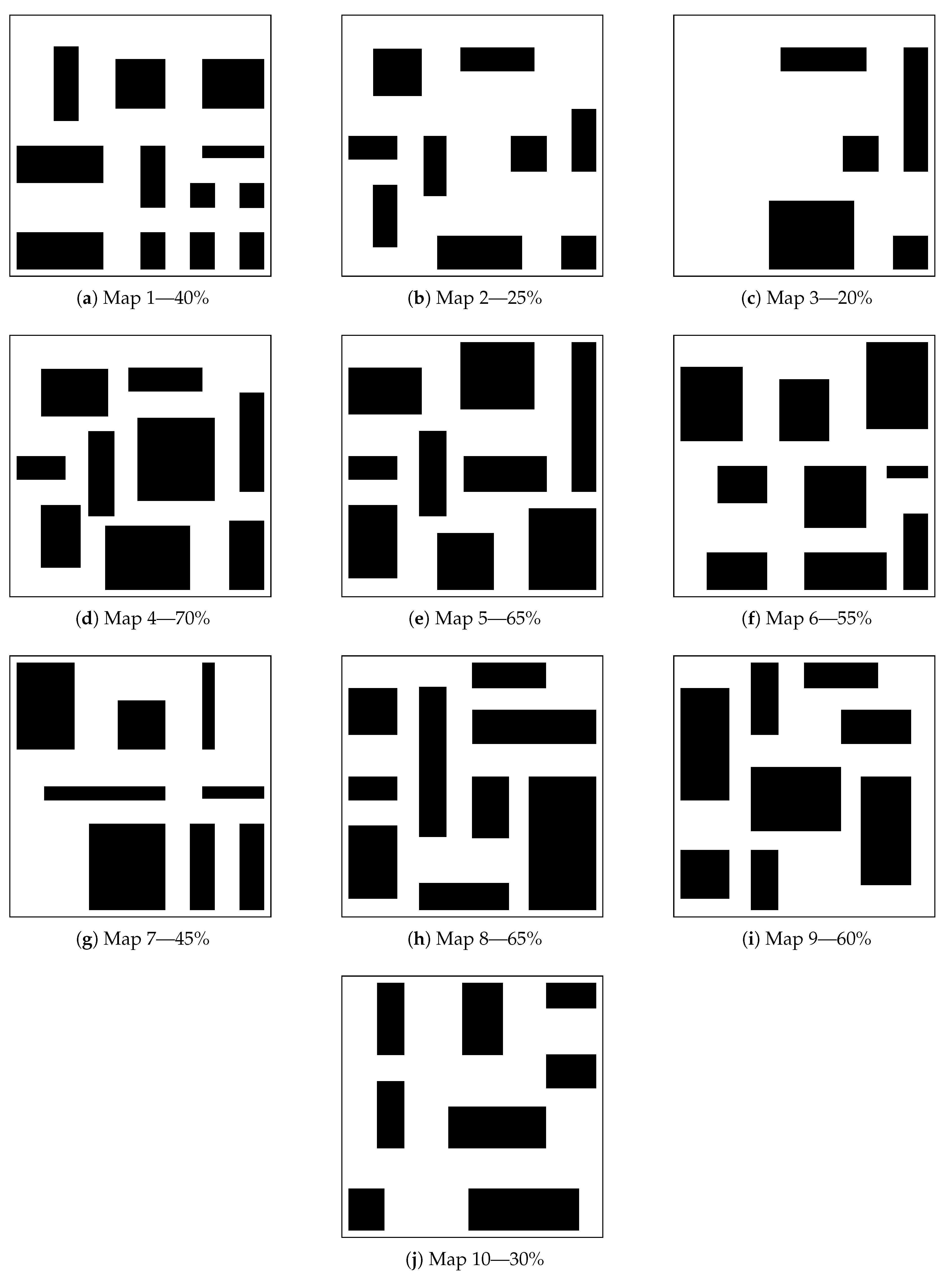
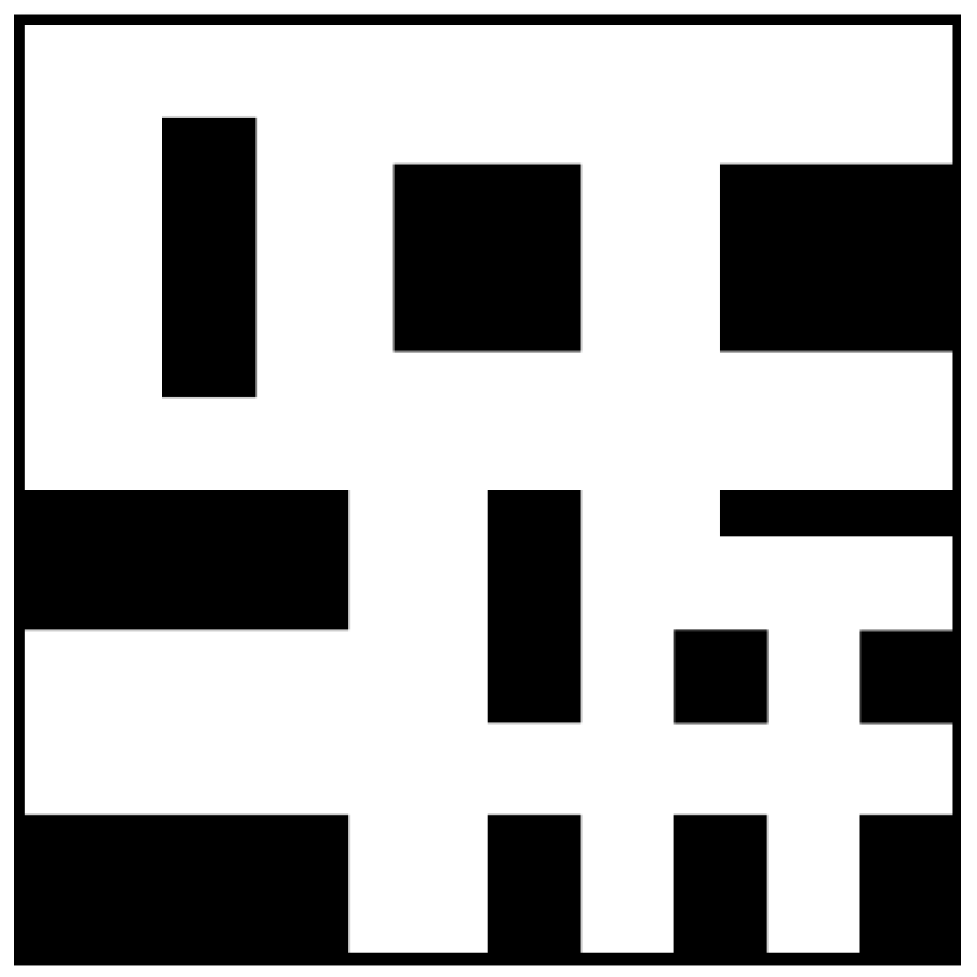
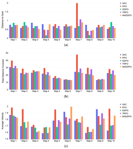
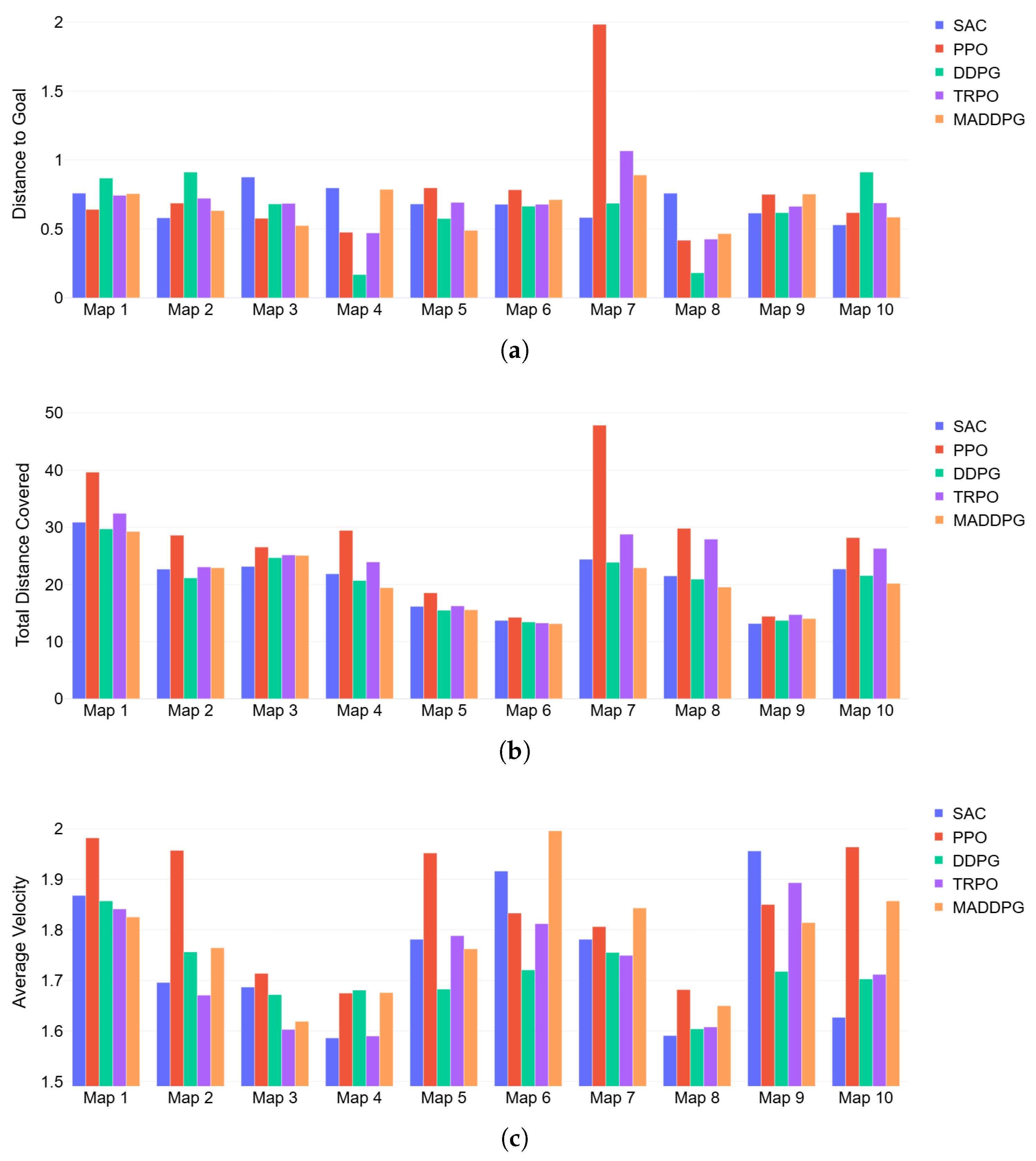
The comparison of all five algorithms across 10 different maps with varying obstacle densities was also carried out in a 2D environment (see Figure 7, Table A5—Distance To Goal, Table A6—Total Distance Covered, Table A7—Average Velocity). The base maps used in this comparison are provided in Figure A1. The distance to the goal remained consistent for all five algorithms across most maps, reflecting their ability to effectively guide agents toward their respective targets. This consistency was expected, as all algorithms were trained with the same goal-oriented reward functions. However, a notable exception occurred in Map 7, where one of the PPO agents got stuck in a local minimum before reaching the target. This resulted in a higher distance to the goal for that specific scenario. This failure suggests that PPO may occasionally struggle with obstacle avoidance in high-complexity environments, potentially due to its on-policy learning mechanism, which relies on fresh data and may not generalize well to unexpected scenarios. When evaluating the total distance covered, significant differences emerged among the algorithms. PPO consistently showed the highest total distance covered, followed by TRPO and SAC, with DDPG and MADDPG demonstrating the least total distance covered in almost all maps. A lower total distance covered indicates more efficient navigation, suggesting that DDPG and MADDPG excel in planning and executing shorter and smoother paths to the targets. While lower than DDPG, SAC’s performance was not as bad as PPO’s. It relies on stochastic policies that may prioritize exploration over strict path optimization. PPO’s relatively higher total distance covered is attributed to its exploration-heavy approach, which, while beneficial for learning diverse policies, may lead to inefficient trajectories in well-trained scenarios. In terms of average velocity, all five algorithms performed comparably, with PPO showing slightly higher average velocity in most cases. This result aligns with its tendency to take longer paths, as a higher velocity might compensate for increased travel distances to complete the navigation within the episode’s time constraints. TRPO, DDPG, MADDPG, and SAC showed similar velocities, indicating a balance between their trajectory planning and movement efficiency. However, in the case of DDPG and MADDPG, a combination of shorter paths and moderate velocity reinforces their overall superiority. It is also important to note here that the results across these metrics remained largely consistent across both 2D and 3D environments.

Figure 7. Comparison of SAC, PPO, DDPG, TRPO, and MADDPG across 10 maps with varying obstacle coverage based on distance to the goal, total distance covered, and average velocity in a 2D environment. (a) distance to goal, (b) total distance covered, (c) average velocity.

5.2. U3D Map Results

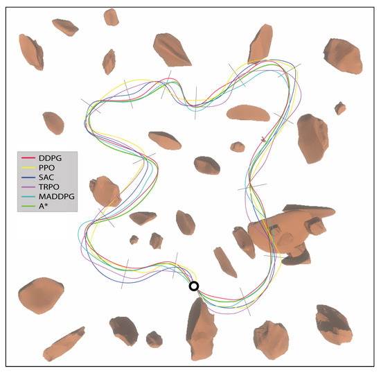
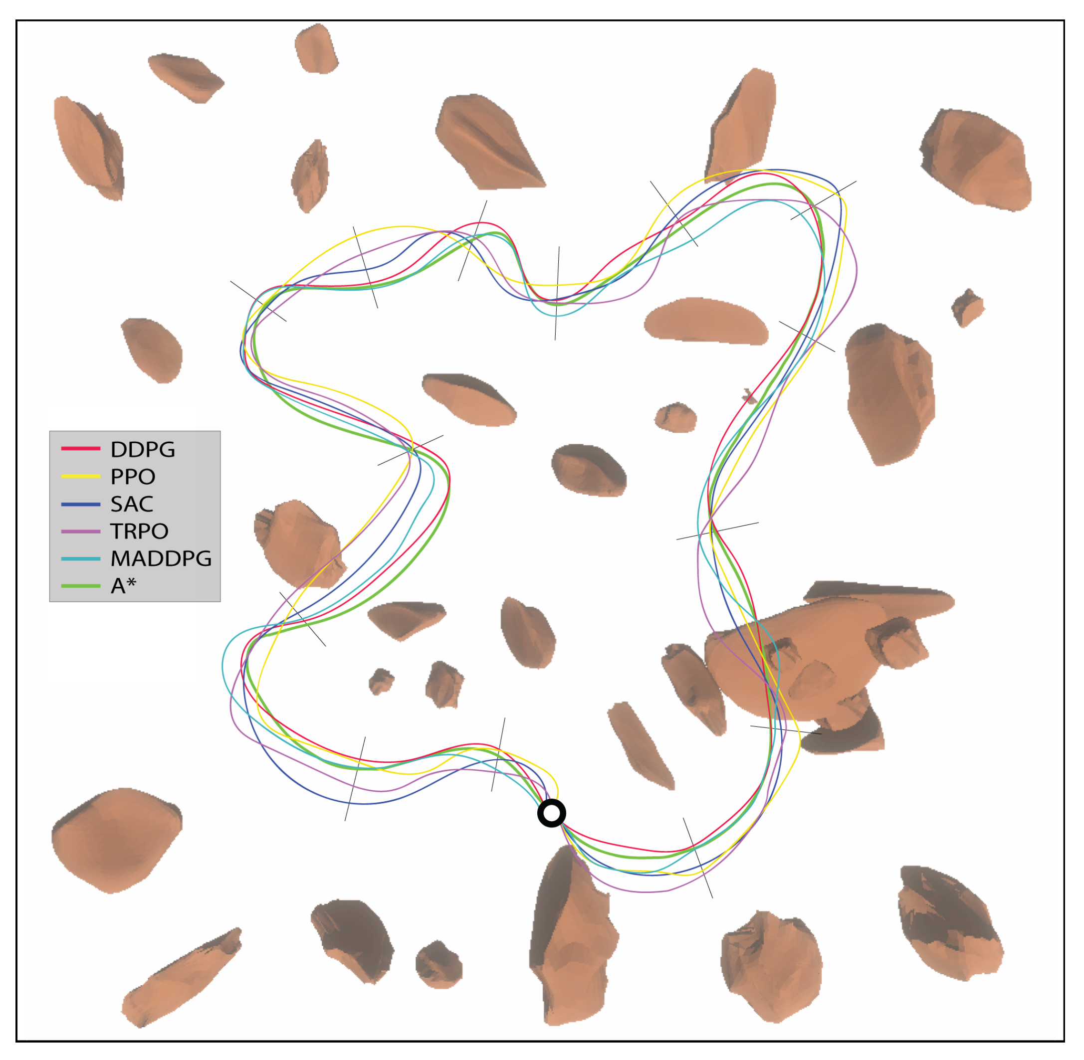
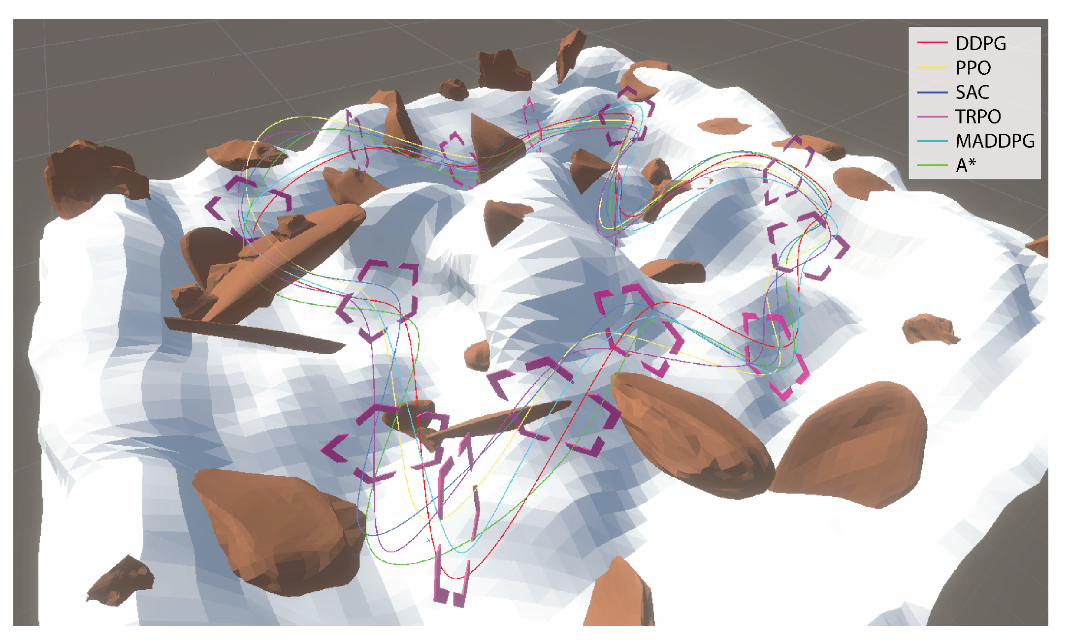
To evaluate and verify the performance of all three algorithms in a 3D environment, a physics-based simulator was used, where a scenario of UAV racing was planned with the UAVs passing through multiple checkpoints (as depicted in Figure 8 and Figure 9). The transition from 2D to 3D environments introduced significant challenges for all algorithms, including the need to account for height variations and the physical engine. DDPG and MADDPG retained their performance advantage, effectively using their continuous action space representation to navigate in three dimensions. SAC showed moderate adaptability but required more training iterations to achieve comparable performance. PPO and TRPO faced difficulties in maintaining stability under 3D dynamics, resulting in reduced efficiency and higher collision rates. These findings highlight the significance of algorithm design choices, such as deterministic versus stochastic policies and on-policy versus off-policy learning, in addressing the complexities of multidimensional environments. Overall, the deterministic policy and replay buffer for DDPG and MADDPG made them particularly well suited for high-dimensional, physics-based environments, aligning with the requirements of UAV swarm navigation tasks.

Figure 8. Top down projections of the 3D trajectories of DDPG, PPO, SAC, TRPO, and MADDPG in U3D environment [59], along with the reference A* trajectory and 14 checkpoints.

Figure 9. Side view of the 3D trajectories of DDPG, PPO, SAC, TRPO, and MADDPG in U3D environment [59], along with the reference A* trajectory and 14 checkpoints.

Table 5 compares all five algorithms in terms of average task completion time, obstacles hitting probability, and average rewards, along with their standard deviations. These results demonstrate that DDPG and MADDPG outperformed the other three algorithms in average time to completed all checkpoints (with the checkpoint-wise performance shown in Table A1) and obstacle-hitting probability. MADDPG also achieved the highest average reward, indicating its superior ability to learn efficient and safe navigation strategies.

Table 5. Performance metrics (mean ± standard deviation) across algorithms in three-dimensional Unity environment.

Algorithm	Avg. Time to Complete (s)	Obstacle-Hitting Prob. (%)	Avg. Reward
DDPG	1241.34 (±32.51)	14.18 (±1.73)	168.24 (±5.42)
SAC	1425.67 (±28.17)	16.58 (±2.01)	158.26 (±4.96)
PPO	1438.16 (±31.45)	22.43 (±2.44)	134.17 (±6.21)
TRPO	1340.90 (±29.64)	17.12 (±1.91)	150.35 (±4.78)
MADDPG	1258.05 (±28.26)	13.96 (±1.48)	172.51 (±4.34)

Table 6 contains the results for three key metrics: total distance covered (TDC), distance to coal (DTG), and average velocity (AV) in the 3D environment, along with their respective standard deviations. Each metric reflects a unique aspect of the algorithms’ effectiveness in a multi-agent UAV path planning under realistic conditions. DDPG and MADDPG showed the least total distance covered, indicating that they are the most efficient algorithms for path optimization (see Table A2). This suggests that they effectively balance exploration and exploitation to find shorter, more direct routes. SAC and PPO covered significantly longer distances, with PPO having the highest total distance. This implies less efficient pathfinding due to higher exploration tendencies and suboptimal policy convergence in the complex dynamics of a 3D environment. All five algorithms achieved similar final distances to the goal, with PPO performing slightly better than the other four algorithms. This indicates that PPO is better at honing in on the exact goal location by the end of each episode. PPO also achieved the highest average velocity, followed by SAC, TRPO, MADDPG, and DDPG (as seen in Table 6). This indicates that PPO prioritizes higher speeds and is also more efficient, likely contributing to its slightly better goal precision but at the expense of longer paths and potentially higher energy consumption. DDPG, with the lowest velocity, maintained a more conservative and calculated pace. This aligns with its optimized path and lower total distance, resulting in improved energy efficiency. The tradeoff between velocity and efficiency is evident here. PPO’s higher velocity led to more energy consumption and overshooting checkpoints, whereas controlled velocities for DDPG and MADDPG resulted in smoother navigation and lower energy costs. These two appear to be the most suitable algorithms for scenarios prioritizing energy efficiency and path optimization. They remain ideal for missions where resource constraints are critical, such as long-term surveillance or search-and-rescue operations.

Table 6. Total distance covered, final distance to goal, and average velocity for each algorithm in 3D environment. Values are reported as mean ± standard deviation over six independent runs to reflect performance variability.

Algorithm	Total Distance Covered	Distance To Goal	Avg. Velocity
DDPG	189.676 (±5.52)	1.712 (±0.084)	15.28 (±0.37)
SAC	230.103 (±6.34)	1.689 (±0.073)	16.14 (±0.29)
PPO	240.604 (±7.18)	1.542 (±0.069)	16.73 (±0.31)
TRPO	207.127 (±6.93)	1.628 (±0.075)	15.56 (±0.34)
MADDPG	193.668 (±5.20)	1.613 (±0.081)	15.34 (±0.28)

5.3. Training Processes

We conducted a comparative analysis for the training behavior of all RL algorithms in both P2D and U3D environments. This comparison includes convergence rates, average training time in hours, total number of steps to convergence, reward per 10,000 steps, and reward standard deviation. These metrics for both environments are detailed in Table 7.

Table 7. Training process comparison for all five algorithms in both P2D and U3D environments.

Env	Algorithm	Convergence Episodes	Training Time (h)	Steps to Converge	Reward/ 10k Steps	Reward Std. Dev.
P2D	DDPG	561	13.61	206,571	6.501	±3.15
P2D	SAC	358	10.68	127,865	6.917	±2.79
P2D	PPO	714	17.13	265,481	5.664	±3.82
P2D	TRPO	642	14.55	238,037	5.691	±3.76
P2D	MADDPG	579	13.94	215,492	6.479	±3.02
U3D	DDPG	1496	54.78	1,171,014	1.436	±5.42
U3D	SAC	1067	47.96	855,391	1.850	±4.96
U3D	PPO	2102	56.51	1,606,507	0.835	±6.21
U3D	TRPO	1983	53.62	1,417,086	1.060	±5.88
U3D	MADDPG	1524	55.40	1,229,354	1.403	±5.25

SAC demonstrated faster convergence across both environments due to its entropy-regularized objective, which balanced exploration and exploitation more effectively. This aligns with the findings of Haarnoja et al. [60], empirically demonstrating that entropy regularization in SAC leads to improved sample efficiency and faster convergence compared to other SOTA methods across multiple continuous control tasks. PPO and TRPO, being on-policy methods, required significantly more samples to converge. DDPG and MADDPG converged faster than PPO and TRPO in both environments, but were more sensitive to hyperparameter tuning. The reward stability, reflected by the standard deviation across six independent training runs, was highest (lowest deviation) for SAC in both environments. TRPO in P2D converged faster than PPO but was unable to surpass the general performance of both SAC and DDPG.

Through empirical experimentation, we observed that DDPG and TRPO were specifically sensitive to the learning rate and noise parameters. A slight increase in the actor learning rate from 0.001 to 0.01 in DDPG led to training divergence in over 60% of runs. Similarly, for TRPO, improper tuning of the KL-divergence constraint led to poor convergence, particularly in the U3D environment, where spatial dynamics are more complex. SAC and PPO required tuning for the temperature (entropy coefficient) and clipping ratio, respectively. Increasing PPO’s clipping parameter from 0.2 to 0.3 led to a 9% reduction in the final target-reaching accuracy in P2D. On the other hand, MADDPG, being a multi-agent extension, required fine-tuning of not just the learning rates but also the exploration noise for each agent. Improper noise scheduling in MADDPG resulted in frequent inter-agent collisions during early training epochs.

We observed that PPO exhibited a relatively higher standard deviation across both environments and most performance metrics. This variability can be attributed to the nature of PPO’s clipped surrogate objective, which attempts to balance exploration and exploitation through conservative updates. In highly dynamic and cluttered multi-agent scenarios, conservative updates occasionally fail to converge to stable policies, particularly when reward gradients fluctuate due to frequent obstacle interactions or sudden changes in spatial constraints. PPO’s reliance on mini-batch training can introduce further performance fluctuations when the training data distribution is not representative of the full state space. This results in a higher degree of performance variance across independent runs. In contrast, SAC utilizes entropy regularization for consistent exploration, whereas DDPG uses soft target updates and a separate target network (for both actor and critic). This helps stabilize learning by smoothing out fluctuations in both cases. These findings highlight that while PPO can perform competitively in terms of mean performance, its variance profile needs to be carefully considered in real-world deployments.

5.4. Discussion

Across all experiments conducted in both P2D and U3D environments, consistent trends emerged regarding the strengths and limitations of each algorithm. DDPG and MADDPG consistently outperformed other approaches in terms of path efficiency and obstacle avoidance. Their deterministic policies enabled smoother trajectories and minimal deviation, making them particularly effective in scenarios demanding precise navigation.

SAC, while not as optimal as DDPG and MADDPG in trajectory planning, offered a strong balance between exploration and performance. Its stochastic nature facilitated better adaptability in unfamiliar or changing environments, although it occasionally resulted in inefficient detours. PPO and TRPO, on the other hand, tended to struggle in highly complex or dynamic scenarios. The clipped surrogate objective of PPO stabilized training but restricted fine-tuning capabilities, often leading to suboptimal paths and higher obstacle collision probability, especially in tightly packed environments. DDPG’s lower total distance covered, coupled with moderate and consistent average velocities, highlights its superior planning abilities. SAC exhibited a competitive yet slightly more exploratory behavior, whereas PPO’s high velocity and longer trajectories suggest a reactive, rather than predictive, pattern. DDPG and MADDPG demonstrated consistent and reliable performance across different swarm sizes, environments, and maps, making them suitable choices for real-time autonomous swarm navigation in structured and semi-structured scenarios. SAC and TRPO may serve as strong alternatives in situations requiring adaptive exploration and sample efficiency, respectively. On the contrary, PPO may need further tuning or hybrid integration to improve its performance in complex, obstacle-rich domains.

Our results underline the significant potential of RL algorithms in enabling autonomous UAV swarm navigation under complex scenarios. The performance advantages of policy-gradient methods stem from their ability to learn precise and efficient policies, particularly in dynamic and high-dimensional environments. While SAC and PPO do provide robustness and stability, their performance in scenarios requiring rapid decision making and adaptability is limited compared to DDPG or MADDPG.

6. Conclusions

In this study, we investigated the applications of RL algorithms for navigating UAV swarms in complex environments. We focused on evaluating the performance of five RL algorithms—SAC, PPO, TRPO, DDPG, and MADDPG—in a scenario where multiple autonomous UAVs must navigate through unknown environments with obstacles and reach designated targets as efficiently as possible. Our findings indicate that each algorithm demonstrates unique strengths and limitations in terms of stability, sample efficiency, and adaptability to the dynamic nature of the environment. With its maximum entropy approach, SAC and TRPO proved effective in promoting exploration and maintaining stability, although they exhibited slower convergence in scenarios that required precise and rapid decisions. PPO, known for its simplicity and stability, faced challenges in environments that required rapid adaptation. DDPG and MADDPG, having an off-policy nature and deterministic policies, excelled in continuous action spaces and became the best-performing algorithms across multiple metrics.

The results highlight the potential of RL-based solutions in UAV swarm navigation, offering a promising approach to autonomously navigating complex environments with obstacles. Using RL-based solutions, UAV swarms can continuously improve their decision-making processes, adapt to new situations, and enhance their overall performance. These capabilities are crucial in search and rescue, environmental monitoring, and disaster response, where rapid, accurate, and coordinated actions are essential. While there are still challenges to overcome, such as the computational demands of specific algorithms and the need for real-time decision making, the success of RL in these applications underscores its significant potential in advancing autonomous UAV swarm technologies.

Future work should focus on refining these algorithms for improved real-time performance, exploring hybrid approaches, investigating how these algorithms scale in various training paradigms, and expanding the applicability of RL to more complex and dynamic environments. Our findings suggest that algorithm selection should be tailored to the specific demands of the application. However, one of the key limitations of the current study is the simulation-driven nature of the experiments; transferring these models to real-world UAV hardware presents challenges related to sensor noise, communication delays, and physical dynamics mismatches. Addressing these issues through sim-to-real transfer techniques and hardware-in-the-loop testing will be important. Additionally, further research is needed to explore the effects of training approaches and swarm size on coordination complexity and performance bottlenecks, as well as to incorporate the combination of centralized, decentralized, and federated training and learning paradigms to improve swarm performance.

Appendix A.1. Time Taken to Reach Checkpoints

Table A1. Time taken to reach respective checkpoints in the 3D environment for all 5 algorithms.

Checkpoint	DDPG	SAC	PPO	TRPO	MADDPG
CP1	84.96	97.19	108.06	96.13	85.28
CP2	90.76	105.24	112.39	101.78	92.57
CP3	89.30	104.40	97.42	94.61	91.06
CP4	105.93	120.52	126.65	107.38	106.12
CP5	87.79	102.33	106.83	93.09	88.91
CP6	93.29	108.45	115.62	103.66	95.17
CP7	91.14	106.78	112.17	98.34	93.65
CP8	65.82	78.42	61.93	68.02	66.81
CP9	72.61	79.56	84.81	76.85	70.04
CP10	71.48	85.89	83.38	80.40	74.56
CP11	104.26	118.73	124.16	109.47	107.87
CP12	109.67	124.39	129.94	119.36	102.82
CP13	96.52	104.28	93.67	107.55	99.64
CP14	77.81	89.49	81.13	84.26	83.55
Total	1241.34	1425.67	1438.16	1340.90	1258.05

Table A1. Time taken to reach respective checkpoints in the 3D environment for all 5 algorithms.

Checkpoint	DDPG	SAC	PPO	TRPO	MADDPG
CP1	84.96	97.19	108.06	96.13	85.28
CP2	90.76	105.24	112.39	101.78	92.57
CP3	89.30	104.40	97.42	94.61	91.06
CP4	105.93	120.52	126.65	107.38	106.12
CP5	87.79	102.33	106.83	93.09	88.91
CP6	93.29	108.45	115.62	103.66	95.17
CP7	91.14	106.78	112.17	98.34	93.65
CP8	65.82	78.42	61.93	68.02	66.81
CP9	72.61	79.56	84.81	76.85	70.04
CP10	71.48	85.89	83.38	80.40	74.56
CP11	104.26	118.73	124.16	109.47	107.87
CP12	109.67	124.39	129.94	119.36	102.82
CP13	96.52	104.28	93.67	107.55	99.64
CP14	77.81	89.49	81.13	84.26	83.55
Total	1241.34	1425.67	1438.16	1340.90	1258.05

Appendix A.2. Total Distance Covered

Table A2. Distance covered while traversing from one checkpoint to the next for each section of the 3D course for all five algorithms.

Checkpoint	DDPG	SAC	PPO	TRPO	MADDPG
CP1	12.981	15.686	18.078	13.782	13.122
CP2	13.868	16.985	18.802	14.897	13.619
CP3	13.645	16.850	16.298	15.913	14.907
CP4	16.186	19.451	21.188	17.325	16.334
CP5	13.414	16.516	17.872	14.695	13.145
CP6	14.254	17.503	19.343	16.591	14.403
CP7	13.926	17.234	18.766	14.163	15.132
CP8	10.057	12.656	10.360	11.740	10.223
CP9	11.094	12.840	14.188	10.703	11.172
CP10	10.922	13.862	13.949	12.991	10.774
CP11	15.930	19.163	20.771	17.102	15.712
CP12	16.757	20.076	21.738	17.011	16.953
CP13	14.748	16.830	15.670	16.651	14.629
CP14	11.889	14.443	13.573	13.563	13.543
Total	189.676	230.103	240.604	207.127	193.668

Table A2. Distance covered while traversing from one checkpoint to the next for each section of the 3D course for all five algorithms.

Checkpoint	DDPG	SAC	PPO	TRPO	MADDPG
CP1	12.981	15.686	18.078	13.782	13.122
CP2	13.868	16.985	18.802	14.897	13.619
CP3	13.645	16.850	16.298	15.913	14.907
CP4	16.186	19.451	21.188	17.325	16.334
CP5	13.414	16.516	17.872	14.695	13.145
CP6	14.254	17.503	19.343	16.591	14.403
CP7	13.926	17.234	18.766	14.163	15.132
CP8	10.057	12.656	10.360	11.740	10.223
CP9	11.094	12.840	14.188	10.703	11.172
CP10	10.922	13.862	13.949	12.991	10.774
CP11	15.930	19.163	20.771	17.102	15.712
CP12	16.757	20.076	21.738	17.011	16.953
CP13	14.748	16.830	15.670	16.651	14.629
CP14	11.889	14.443	13.573	13.563	13.543
Total	189.676	230.103	240.604	207.127	193.668

Appendix B.1. 10-UAV Swarm Results

Table A3. Total time (in seconds), number of steps, and obstacle-hitting probabilities for a 10-UAV swarm in a two-dimensional Python environment. ‘X’ indicates a crash (with an obstacle or another UAV), while ‘∞’ indicates a UAV stuck hovering until the episode ends.

		SAC	PPO	DDPG	TRPO	MADDPG
UAV 1	Time (s)	115	97	104	106	92
	Steps	99	103	96	102	94
UAV 2	Time (s)	101	101	81	98	83
	Steps	87	112	79	93	82
UAV 3	Time (s)	∞	103	116	138	124
	Steps	∞	124	133	166	128
UAV 4	Time (s)	101	82	98	117	92
	Steps	95	82	90	107	93
UAV 5	Time (s)	122	134	97	112	100
	Steps	111	118	105	129	104
UAV 6	Time (s)	116	129	88	111	99
	Steps	114	133	107	105	103
UAV 7	Time (s)	X	143	X	97	121
	Steps	X	139	X	101	122
UAV 8	Time (s)	X	∞	X	126	X
	Steps	X	∞	X	129	X
UAV 9	Time (s)	∞	∞	∞	∞	∞
	Steps	∞	∞	∞	∞	∞
UAV 10	Time (s)	101	∞	97	101	103
	Steps	113	∞	103	107	101
Obstacle-Hitting Probability		∼18%	∼43%	∼17%	∼25%	∼15%

Table A3. Total time (in seconds), number of steps, and obstacle-hitting probabilities for a 10-UAV swarm in a two-dimensional Python environment. ‘X’ indicates a crash (with an obstacle or another UAV), while ‘∞’ indicates a UAV stuck hovering until the episode ends.

		SAC	PPO	DDPG	TRPO	MADDPG
UAV 1	Time (s)	115	97	104	106	92
	Steps	99	103	96	102	94
UAV 2	Time (s)	101	101	81	98	83
	Steps	87	112	79	93	82
UAV 3	Time (s)	∞	103	116	138	124
	Steps	∞	124	133	166	128
UAV 4	Time (s)	101	82	98	117	92
	Steps	95	82	90	107	93
UAV 5	Time (s)	122	134	97	112	100
	Steps	111	118	105	129	104
UAV 6	Time (s)	116	129	88	111	99
	Steps	114	133	107	105	103
UAV 7	Time (s)	X	143	X	97	121
	Steps	X	139	X	101	122
UAV 8	Time (s)	X	∞	X	126	X
	Steps	X	∞	X	129	X
UAV 9	Time (s)	∞	∞	∞	∞	∞
	Steps	∞	∞	∞	∞	∞
UAV 10	Time (s)	101	∞	97	101	103
	Steps	113	∞	103	107	101
Obstacle-Hitting Probability		∼18%	∼43%	∼17%	∼25%	∼15%

Appendix B.2. 20-UAV Swarm Results

Table A4. Total time (in seconds), number of steps, and obstacle-hitting probabilities for a 20-UAV swarm in a two-dimensional Python environment. ‘X’ indicates a crash (with an obstacle or another UAV), while ‘∞’ indicates a UAV stuck hovering until the episode ends.

		SAC	PPO	DDPG	TRPO	MADDPG
UAV 1	Time (s)	113	95	107	104	99
	Steps	101	105	98	106	102
UAV 2	Time (s)	100	103	82	99	84
	Steps	89	115	81	94	85
UAV 3	Time (s)	∞	103	116	138	124
	Steps	∞	127	134	167	129
UAV 4	Time (s)	103	84	99	116	96
	Steps	98	86	94	112	95
UAV 5	Time (s)	124	132	96	113	97
	Steps	110	119	104	128	100
UAV 6	Time (s)	117	131	87	114	103
	Steps	113	136	108	106	104
UAV 7	Time (s)	X	144	X	99	122
	Steps	X	140	X	104	129
UAV 8	Time (s)	X	∞	X	128	X
	Steps	X	∞	X	131	X
UAV 9	Time (s)	∞	∞	∞	∞	∞
	Steps	∞	∞	∞	∞	∞
UAV 10	Time (s)	104	∞	98	103	110
	Steps	117	∞	109	113	113
UAV 11	Time (s)	124	∞	125	119	127
	Steps	139	∞	134	128	126
UAV 12	Time (s)	106	132	105	113	108
	Steps	110	127	109	117	104
UAV 13	Time (s)	105	122	107	119	109
	Steps	111	119	112	123	116
UAV 14	Time (s)	72	79	72	77	86
	Steps	79	77	81	80	88
UAV 15	Time (s)	93	107	92	101	88
	Steps	97	102	94	109	89
UAV 16	Time (s)	118	136	118	117	122
	Steps	124	131	122	120	124
UAV 17	Time (s)	∞	142	∞	∞	∞
	Steps	∞	138	∞	∞	∞
UAV 18	Time (s)	99	113	98	94	105
	Steps	106	106	104	101	104
UAV 19	Time (s)	113	104	112	115	113
	Steps	121	99	119	125	115
UAV 20	Time (s)	93	87	97	94	103
	Steps	104	84	108	105	112
Obstacle-Hitting Probability		∼21%	∼49%	∼19%	∼28%	∼18%

Table A4. Total time (in seconds), number of steps, and obstacle-hitting probabilities for a 20-UAV swarm in a two-dimensional Python environment. ‘X’ indicates a crash (with an obstacle or another UAV), while ‘∞’ indicates a UAV stuck hovering until the episode ends.

		SAC	PPO	DDPG	TRPO	MADDPG
UAV 1	Time (s)	113	95	107	104	99
	Steps	101	105	98	106	102
UAV 2	Time (s)	100	103	82	99	84
	Steps	89	115	81	94	85
UAV 3	Time (s)	∞	103	116	138	124
	Steps	∞	127	134	167	129
UAV 4	Time (s)	103	84	99	116	96
	Steps	98	86	94	112	95
UAV 5	Time (s)	124	132	96	113	97
	Steps	110	119	104	128	100
UAV 6	Time (s)	117	131	87	114	103
	Steps	113	136	108	106	104
UAV 7	Time (s)	X	144	X	99	122
	Steps	X	140	X	104	129
UAV 8	Time (s)	X	∞	X	128	X
	Steps	X	∞	X	131	X
UAV 9	Time (s)	∞	∞	∞	∞	∞
	Steps	∞	∞	∞	∞	∞
UAV 10	Time (s)	104	∞	98	103	110
	Steps	117	∞	109	113	113
UAV 11	Time (s)	124	∞	125	119	127
	Steps	139	∞	134	128	126
UAV 12	Time (s)	106	132	105	113	108
	Steps	110	127	109	117	104
UAV 13	Time (s)	105	122	107	119	109
	Steps	111	119	112	123	116
UAV 14	Time (s)	72	79	72	77	86
	Steps	79	77	81	80	88
UAV 15	Time (s)	93	107	92	101	88
	Steps	97	102	94	109	89
UAV 16	Time (s)	118	136	118	117	122
	Steps	124	131	122	120	124
UAV 17	Time (s)	∞	142	∞	∞	∞
	Steps	∞	138	∞	∞	∞
UAV 18	Time (s)	99	113	98	94	105
	Steps	106	106	104	101	104
UAV 19	Time (s)	113	104	112	115	113
	Steps	121	99	119	125	115
UAV 20	Time (s)	93	87	97	94	103
	Steps	104	84	108	105	112
Obstacle-Hitting Probability		∼21%	∼49%	∼19%	∼28%	∼18%

Appendix B.3. Distance to Goal

Table A5. Final distance to the goal for each algorithm in the 2D environment across 10 different maps with varying obstacle coverage.

Map Number	Obstacle Coverage	SAC	PPO	DDPG	TRPO	MADDPG
Map 1	40%	0.760	0.641	0.869	0.744	0.756
Map 2	25%	0.581	0.687	0.912	0.722	0.633
Map 3	40%	0.876	0.577	0.681	0.685	0.524
Map 4	70%	0.798	0.476	0.169	0.471	0.787
Map 5	65%	0.681	0.798	0.576	0.692	0.490
Map 6	55%	0.679	0.784	0.665	0.679	0.712
Map 7	45%	0.583	1.984	0.686	1.066	0.891
Map 8	65%	0.759	0.418	0.182	0.426	0.466
Map 9	60%	0.615	0.751	0.618	0.664	0.753
Map 10	30%	0.529	0.618	0.912	0.689	0.586

Table A5. Final distance to the goal for each algorithm in the 2D environment across 10 different maps with varying obstacle coverage.

Map Number	Obstacle Coverage	SAC	PPO	DDPG	TRPO	MADDPG
Map 1	40%	0.760	0.641	0.869	0.744	0.756
Map 2	25%	0.581	0.687	0.912	0.722	0.633
Map 3	40%	0.876	0.577	0.681	0.685	0.524
Map 4	70%	0.798	0.476	0.169	0.471	0.787
Map 5	65%	0.681	0.798	0.576	0.692	0.490
Map 6	55%	0.679	0.784	0.665	0.679	0.712
Map 7	45%	0.583	1.984	0.686	1.066	0.891
Map 8	65%	0.759	0.418	0.182	0.426	0.466
Map 9	60%	0.615	0.751	0.618	0.664	0.753
Map 10	30%	0.529	0.618	0.912	0.689	0.586

Appendix B.4. Total Distance Covered

Table A6. Total distance covered for each algorithm in the 2D environment across 10 different maps with varying obstacle coverage.

Map Number	Obstacle Coverage	SAC	PPO	DDPG	TRPO	MADDPG
Map 1	40%	30.87	39.64	29.71	32.43	29.25
Map 2	25%	22.67	28.59	21.12	23.04	22.91
Map 3	40%	23.14	26.52	24.68	25.16	25.07
Map 4	70%	21.84	29.45	20.68	23.93	19.42
Map 5	65%	16.17	18.53	15.48	16.25	15.57
Map 6	55%	13.69	14.25	13.42	13.26	13.12
Map 7	45%	24.39	47.84	23.86	28.77	22.89
Map 8	65%	21.48	29.81	20.91	27.92	19.53
Map 9	60%	13.16	14.41	13.69	14.72	14.02
Map 10	30%	22.68	28.18	21.54	26.28	20.18

Table A6. Total distance covered for each algorithm in the 2D environment across 10 different maps with varying obstacle coverage.

Map Number	Obstacle Coverage	SAC	PPO	DDPG	TRPO	MADDPG
Map 1	40%	30.87	39.64	29.71	32.43	29.25
Map 2	25%	22.67	28.59	21.12	23.04	22.91
Map 3	40%	23.14	26.52	24.68	25.16	25.07
Map 4	70%	21.84	29.45	20.68	23.93	19.42
Map 5	65%	16.17	18.53	15.48	16.25	15.57
Map 6	55%	13.69	14.25	13.42	13.26	13.12
Map 7	45%	24.39	47.84	23.86	28.77	22.89
Map 8	65%	21.48	29.81	20.91	27.92	19.53
Map 9	60%	13.16	14.41	13.69	14.72	14.02
Map 10	30%	22.68	28.18	21.54	26.28	20.18

Appendix B.5. Average Velocity

Table A7. Average velocity for each algorithm in the 2D environment across 10 different maps with varying obstacle coverage.

Map Number	Obstacle Coverage	SAC	PPO	DDPG	TRPO	MADDPG
Map 1	40%	1.868	1.982	1.857	1.841	1.825
Map 2	25%	1.696	1.957	1.756	1.671	1.764
Map 3	40%	1.687	1.714	1.672	1.603	1.619
Map 4	70%	1.586	1.675	1.681	1.590	1.676
Map 5	65%	1.781	1.952	1.683	1.788	1.762
Map 6	55%	1.916	1.833	1.721	1.812	1.996
Map 7	45%	1.781	1.806	1.755	1.749	1.843
Map 8	65%	1.591	1.682	1.604	1.608	1.650
Map 9	60%	1.956	1.850	1.718	1.893	1.814
Map 10	30%	1.627	1.964	1.703	1.712	1.857

Table A7. Average velocity for each algorithm in the 2D environment across 10 different maps with varying obstacle coverage.

Map Number	Obstacle Coverage	SAC	PPO	DDPG	TRPO	MADDPG
Map 1	40%	1.868	1.982	1.857	1.841	1.825
Map 2	25%	1.696	1.957	1.756	1.671	1.764
Map 3	40%	1.687	1.714	1.672	1.603	1.619
Map 4	70%	1.586	1.675	1.681	1.590	1.676
Map 5	65%	1.781	1.952	1.683	1.788	1.762
Map 6	55%	1.916	1.833	1.721	1.812	1.996
Map 7	45%	1.781	1.806	1.755	1.749	1.843
Map 8	65%	1.591	1.682	1.604	1.608	1.650
Map 9	60%	1.956	1.850	1.718	1.893	1.814
Map 10	30%	1.627	1.964	1.703	1.712	1.857

References

- Wan, Y.; Zhong, Y.; Ma, A.; Zhang, L. An accurate UAV 3-D path planning method for disaster emergency response based on an improved multiobjective swarm intelligence algorithm. IEEE Trans. Cybern. 2022, 53, 2658–2671. [Google Scholar] [CrossRef] [Scilit]
- Ruetten, L.; Regis, P.A.; Feil-Seifer, D.; Sengupta, S. Area-Optimized UAV Swarm Network for Search and Rescue Operations. In Proceedings of the 2020 10th Annual Computing and Communication Workshop and Conference (CCWC), Las Vegas, NV, USA, 6–8 January 2020; pp. 0613–0618. [Google Scholar] [CrossRef] [Scilit]
- Arranz, R.; Carramiñana, D.; Miguel, G.d.; Besada, J.A.; Bernardos, A.M. Application of deep reinforcement learning to UAV swarming for ground surveillance. Sensors 2023, 23, 8766. [Google Scholar] [CrossRef] [Scilit]
- Ming, R.; Jiang, R.; Luo, H.; Lai, T.; Guo, E.; Zhou, Z. Comparative Analysis of Different UAV Swarm Control Methods on Unmanned Farms. Agronomy 2023, 13, 2499. [Google Scholar] [CrossRef] [Scilit]
- Awasthi, S.; Fernandez-Cortizas, M.; Reining, C.; Arias-Perez, P.; Luna, M.A.; Perez-Saura, D.; Roidl, M.; Gramse, N.; Klokowski, P.; Campoy, P. Micro UAV Swarm for industrial applications in indoor environment: A systematic literature review. Logist. Res. 2023, 16, 1–43. [Google Scholar]
- Zhu, X. Analysis of military application of UAV swarm technology. In Proceedings of the 2020 3rd International Conference on Unmanned Systems (ICUS), Harbin, China, 27–28 November 2020; pp. 1200–1204. [Google Scholar] [CrossRef] [Scilit]
- Puente-Castro, A.; Rivero, D.; Pazos, A.; Fernandez-Blanco, E. A review of artificial intelligence applied to path planning in UAV swarms. Neural Comput. Appl. 2022, 34, 153–170. [Google Scholar] [CrossRef] [Scilit]
- Madridano, Á.; Al-Kaff, A.; Flores, P.; Martín, D.; de la Escalera, A. Obstacle Avoidance Manager for UAVs Swarm. In Proceedings of the 2020 International Conference on Unmanned Aircraft Systems (ICUAS), Athens, Greece, 1–4 September 2020; pp. 815–821. [Google Scholar] [CrossRef] [Scilit]
- Zhang, X.; Duan, L. Energy-Saving Deployment Algorithms of UAV Swarm for Sustainable Wireless Coverage. IEEE Trans. Veh. Technol. 2020, 69, 10320–10335. [Google Scholar] [CrossRef] [Scilit]
- Dui, H.; Zhang, C.; Bai, G.; Chen, L. Mission reliability modeling of UAV swarm and its structure optimization based on importance measure. Reliab. Eng. Syst. Saf. 2021, 215, 107879. [Google Scholar] [CrossRef] [Scilit]
- Hu, J.; Fan, L.; Lei, Y.; Xu, Z.; Fu, W.; Xu, G. Reinforcement Learning-Based Low-Altitude Path Planning for UAS Swarm in Diverse Threat Environments. Drones 2023, 7, 567. [Google Scholar] [CrossRef] [Scilit]
- Chen, H.; Huang, D.; Wang, C.; Ding, L.; Song, L.; Liu, H. Collision-Free Path Planning for Multiple Drones Based on Safe Reinforcement Learning. Drones 2024, 8, 481. [Google Scholar] [CrossRef] [Scilit]
- Xiong, T.; Liu, F.; Liu, H.; Ge, J.; Li, H.; Ding, K.; Li, Q. Multi-drone optimal mission assignment and 3D path planning for disaster rescue. Drones 2023, 7, 394. [Google Scholar] [CrossRef] [Scilit]
- Huang, H.; Savkin, A.V.; Ni, W. Online UAV trajectory planning for covert video surveillance of mobile targets. IEEE Trans. Autom. Sci. Eng. 2021, 19, 735–746. [Google Scholar] [CrossRef] [Scilit]
- Saunders, J.; Saeedi, S.; Li, W. Autonomous aerial robotics for package delivery: A technical review. J. Field Robot. 2024, 41, 3–49. [Google Scholar] [CrossRef] [Scilit]
- Basiri, A.; Mariani, V.; Silano, G.; Aatif, M.; Iannelli, L.; Glielmo, L. A survey on the application of path-planning algorithms for multi-rotor UAVs in precision agriculture. J. Navig. 2022, 75, 364–383. [Google Scholar] [CrossRef] [Scilit]
- Ortlieb, M.; Adolf, F.M. Rule-based path planning for unmanned aerial vehicles in non-segregated air space over congested areas. In Proceedings of the 2020 AIAA/IEEE 39th Digital Avionics Systems Conference (DASC), San Antonio, TX, USA, 11–15 October 2020; IEEE: New York, NY, USA, 2020; pp. 1–9. [Google Scholar]
- Tan, C.S.; Mohd-Mokhtar, R.; Arshad, M.R. A comprehensive review of coverage path planning in robotics using classical and heuristic algorithms. IEEE Access 2021, 9, 119310–119342. [Google Scholar] [CrossRef] [Scilit]
- Ait Saadi, A.; Soukane, A.; Meraihi, Y.; Benmessaoud Gabis, A.; Mirjalili, S.; Ramdane-Cherif, A. UAV path planning using optimization approaches: A survey. Arch. Comput. Methods Eng. 2022, 29, 4233–4284. [Google Scholar] [CrossRef] [Scilit]
- Afifi, G.; Gadallah, Y. Cellular network-supported machine learning techniques for autonomous UAV trajectory planning. IEEE Access 2022, 10, 131996–132011. [Google Scholar] [CrossRef] [Scilit]
- Bassolillo, S.R.; Raspaolo, G.; Blasi, L.; D’Amato, E.; Notaro, I. Path planning for fixed-wing unmanned aerial vehicles: An integrated approach with theta* and clothoids. Drones 2024, 8, 62. [Google Scholar] [CrossRef] [Scilit]
- Zhang, Z.; Long, T.; Wang, Z.; Xu, G.; Cao, Y. UAV Dynamic Path Planning using Anytime Repairing Sparse A* Algorithm and Targets Motion Estimation (IEEE/CSAA GNCC). In Proceedings of the 2018 IEEE CSAA Guidance, Navigation and Control Conference (CGNCC), Xiamen, China, 10–12 August 2018; IEEE: New York, NY, USA, 2018; pp. 1–6. [Google Scholar]
- Wang, J.; Li, Y.; Li, R.; Chen, H.; Chu, K. Trajectory planning for UAV navigation in dynamic environments with matrix alignment Dijkstra. Soft Comput. 2022, 26, 12599–12610. [Google Scholar] [CrossRef] [Scilit]
- Yang, F.; Fang, X.; Gao, F.; Zhou, X.; Li, H.; Jin, H.; Song, Y. Obstacle avoidance path planning for UAV based on improved RRT algorithm. Discret. Dyn. Nat. Soc. 2022, 2022, 4544499. [Google Scholar] [CrossRef] [Scilit]
- Noreen, I.; Khan, A.; Habib, Z. Optimal path planning using RRT* based approaches: A survey and future directions. Int. J. Adv. Comput. Sci. Appl. 2016, 7, 97–107. [Google Scholar] [CrossRef] [Scilit]
- Pan, Y.; Yang, Y.; Li, W. A deep learning trained by genetic algorithm to improve the efficiency of path planning for data collection with multi-UAV. IEEE Access 2021, 9, 7994–8005. [Google Scholar]
- Phung, M.D.; Ha, Q.P. Safety-enhanced UAV path planning with spherical vector-based particle swarm optimization. Appl. Soft Comput. 2021, 107, 107376. [Google Scholar] [CrossRef] [Scilit]
- Mai, X.; Dong, N.; Liu, S.; Chen, H. UAV path planning based on a dual-strategy ant colony optimization algorithm. Intell. Robot. 2023, 3, 666–684. [Google Scholar] [CrossRef] [Scilit]
- Abro, G.E.M.; Ali, Z.A.; Masood, R.J. Synergistic UAV Motion: A Comprehensive Review on Advancing Multi-Agent Coordination. IECE Trans. Sens. Commun. Control 2024, 1, 72–88. [Google Scholar] [CrossRef] [Scilit]
- Pan, Z.; Zhang, C.; Xia, Y.; Xiong, H.; Shao, X. An improved artificial potential field method for path planning and formation control of the multi-UAV systems. IEEE Trans. Circuits Syst. II Express Briefs 2021, 69, 1129–1133. [Google Scholar] [CrossRef] [Scilit]
- Liu, J.; Yan, Y.; Yang, Y.; Li, J. An improved artificial potential field UAV path planning algorithm guided by RRT under environment-aware modeling: Theory and simulation. IEEE Access 2024, 12, 12080–12097. [Google Scholar] [CrossRef] [Scilit]
- Eser, M.; Yilmaz, A.E. A Gossip-Based Auction Algorithm for Decentralized Task Rescheduling in Heterogeneous Drone Swarms. IEEE Trans. Aerosp. Electron. Syst. 2025. [Google Scholar] [CrossRef] [Scilit]
- Lizzio, F.F.; Capello, E.; Guglieri, G. A review of consensus-based multi-agent UAV implementations. J. Intell. Robot. Syst. 2022, 106, 43. [Google Scholar] [CrossRef] [Scilit]
- Divkoti, M.R.R.; Aguiar, A.P. A Hybrid Learning-Based Path Planning Algorithm for Enhanced Safety in Autonomous Robots. In Proceedings of the APCA International Conference on Automatic Control and Soft Computing, Porto, Portugal, 17–19 July 2024; Springer: Berlin/Heidelberg, Germany, 2024; pp. 198–209. [Google Scholar]
- Ma, H. Graph-based multi-robot path finding and planning. Curr. Robot. Rep. 2022, 3, 77–84. [Google Scholar] [CrossRef] [Scilit]
- Bai, Y.; Kotpalliwar, S.; Kanellakis, C.; Nikolakopoulos, G. Multi-agent Path Planning Based on Conflict-Based Search (CBS) Variations for Heterogeneous Robots. J. Intell. Robot. Syst. 2025, 111, 26. [Google Scholar]
- Chao, Y.; Dillmann, R.; Roennau, A.; Xiong, Z. E-DQN-Based Path Planning Method for Drones in Airsim Simulator under Unknown Environment. Biomimetics 2024, 9, 238. [Google Scholar] [CrossRef] [Scilit] [PubMed]
- Tang, J.; Liang, Y.; Li, K. Dynamic Scene Path Planning of UAVs Based on Deep Reinforcement Learning. Drones 2024, 8, 60. [Google Scholar] [CrossRef] [Scilit]
- Han, L.; Zhang, H.; An, N. A Continuous Space Path Planning Method for Unmanned Aerial Vehicle Based on Particle Swarm Optimization-Enhanced Deep Q-Network. Drones 2025, 9, 122. [Google Scholar] [CrossRef] [Scilit]
- Wang, S.; Qi, N.; Jiang, H.; Xiao, M.; Liu, H.; Jia, L.; Zhao, D. Trajectory planning for uav-assisted data collection in iot network: A double deep q network approach. Electronics 2024, 13, 1592. [Google Scholar] [CrossRef] [Scilit]
- Yang, Y.; Zhang, K.; Liu, D.; Song, H. Autonomous UAV Navigation in Dynamic Environments with Double Deep Q-Networks. In Proceedings of the 2020 AIAA/IEEE 39th Digital Avionics Systems Conference (DASC), San Antonio, TX, USA, 11–15 October 2020; pp. 1–7. [Google Scholar] [CrossRef] [Scilit]
- Ye, B.L.; Zhang, J.; Li, L.; Wu, W. A novel trajectory planning method based on trust region policy optimization. IEEE Trans. Intell. Veh. 2024. [Google Scholar] [CrossRef] [Scilit]
- Hu, D.; Dong, W.; Xie, W.; He, L. Proximal policy optimization for multi-rotor uav autonomous guidance, tracking and obstacle avoidance. Int. J. Aeronaut. Space Sci. 2022, 23, 339–353. [Google Scholar]
- Zhang, D.; Xuan, Z.; Zhang, Y.; Yao, J.; Li, X.; Li, X. Path planning of unmanned aerial vehicle in complex environments based on state-detection twin delayed deep deterministic policy gradient. Machines 2023, 11, 108. [Google Scholar] [CrossRef] [Scilit]
- Zhou, X.; Zhang, X.; Zhao, H.; Xiong, J.; Wei, J. Constrained soft actor-critic for energy-aware trajectory design in UAV-aided IoT networks. IEEE Wirel. Commun. Lett. 2022, 11, 1414–1418. [Google Scholar] [CrossRef] [Scilit]
- Cao, P.; Lei, L.; Cai, S.; Shen, G.; Liu, X.; Wang, X.; Zhang, L.; Zhou, L.; Guizani, M. Computational intelligence algorithms for UAV swarm networking and collaboration: A comprehensive survey and future directions. IEEE Commun. Surv. Tutor. 2024. [Google Scholar] [CrossRef] [Scilit]
- Lowe, R.; Wu, Y.I.; Tamar, A.; Harb, J.; Pieter Abbeel, O.; Mordatch, I. Multi-agent actor-critic for mixed cooperative-competitive environments. Adv. Neural Inf. Process. Syst. 2017, 30. [Google Scholar] [CrossRef] [Scilit]
- Li, W.; Chen, X.; Yu, W.; Xie, M. Multiple unmanned aerial vehicle coordinated strikes against ground targets based on an improved multi-agent deep deterministic policy gradient algorithm. Proc. Inst. Mech. Eng. Part J. Syst. Control Eng. 2024. [Google Scholar] [CrossRef] [Scilit]
- Garg, A.; Jha, S.S. Deep deterministic policy gradient based multi-UAV control for moving convoy tracking. Eng. Appl. Artif. Intell. 2023, 126, 107099. [Google Scholar] [CrossRef] [Scilit]
- Zhang, C.; Wu, Z.; Li, Z.; Xu, H.; Xue, Z.; Qian, R. Multi-agent Reinforcement Learning-Based UAV Swarm Confrontation: Integrating QMIX Algorithm with Artificial Potential Field Method. In Proceedings of the 2024 IEEE International Conference on Systems, Man, and Cybernetics (SMC), Sarawak, Malaysia, 6–10 October 2024; IEEE: New York, NY, USA, 2024; pp. 161–166. [Google Scholar]
- Huang, S.; Zhang, H.; Huang, Z. Multi-UAV collision avoidance using multi-agent reinforcement learning with counterfactual credit assignment. arXiv 2022, arXiv:2204.08594. [Google Scholar]
- Azzam, R.; Chehadeh, M.; Hay, O.A.; Boiko, I.; Zweiri, Y. Learning to Navigate Through Reinforcement Across the Sim2Real Gap. TechRxiv 2022. [Google Scholar] [CrossRef] [Scilit]
- Alpdemir, M.N. A Hierarchical Reinforcement Learning Framework for UAV Path Planning in Tactical Environments. Turk. J. Sci. Technol. 2023, 18, 243–259. [Google Scholar] [CrossRef] [Scilit]
- Samaniego, F.; Sanchis, J.; García-Nieto, S.; Simarro, R. Recursive rewarding modified adaptive cell decomposition (RR-MACD): A dynamic path planning algorithm for UAVs. Electronics 2019, 8, 306. [Google Scholar] [CrossRef] [Scilit]
- Xi, M.; Dai, H.; He, J.; Li, W.; Wen, J.; Xiao, S.; Yang, J. A lightweight reinforcement-learning-based real-time path-planning method for unmanned aerial vehicles. IEEE Internet Things J. 2024, 11, 21061–21071. [Google Scholar] [CrossRef] [Scilit]
- Imanberdiyev, N.; Fu, C.; Kayacan, E.; Chen, I.M. Autonomous navigation of UAV by using real-time model-based reinforcement learning. In Proceedings of the 2016 14th International Conference on Control, Automation, Robotics and Vision (ICARCV), Phuket, Thailand, 13–15 November 2016; IEEE: New York, NY, USA, 2016; pp. 1–6. [Google Scholar]
- Wang, X.; Gursoy, M.C. Resilient path planning for UAVs in data collection under adversarial attacks. IEEE Trans. Inf. Forensics Secur. 2023, 18, 2766–2779. [Google Scholar]
- Ramos, G.S.; Henriques, F.D.R.; Haddad, D.B.; Andrade, F.A.; Pinto, M.F. ARCog-NET: An Aerial Robot Cognitive Network Architecture for Swarm Applications Development. IEEE Access 2024, 12, 129040–129063. [Google Scholar] [CrossRef] [Scilit]
- Kelly, A. Reinforcement Learning: AI Flight with Unity ML-Agents. 2023. Available online: https://www.udemy.com/course/ai-flight/ (accessed on 13 September 2024).
- Haarnoja, T.; Zhou, A.; Abbeel, P.; Levine, S. Soft actor-critic: Off-policy maximum entropy deep reinforcement learning with a stochastic actor. In Proceedings of the International Conference on Machine Learning, PMLR, Stockholm, Sweden, 10–15 July 2018; pp. 1861–1870. [Google Scholar]
Disclaimer/Publisher’s Note: The statements, opinions and data contained in all publications are solely those of the individual author(s) and contributor(s) and not of MDPI and/or the editor(s). MDPI and/or the editor(s) disclaim responsibility for any injury to people or property resulting from any ideas, methods, instructions or products referred to in the content. |
© 2025 by the authors. Licensee MDPI, Basel, Switzerland. This article is an open access article distributed under the terms and conditions of the Creative Commons Attribution (CC BY) license (https://creativecommons.org/licenses/by/4.0/).