Solvability and Stability Analysis of Three-Dimensional ABC Fractional Systems in Locally Compact Hausdorff Spaces: Applications to Chaotic and Fluid Systems

Abstract

This paper considers a general three-dimensional ABC fractional dynamical system formulated in a bounded locally compact Hausdorff space. The locally compact Hausdorff structure ensures that the compact-open topology on the space of continuous functions coincides with the topology induced by the supremum norm, providing an appropriate Banach space framework for the analysis of the system. Within this setting we study the continuity, boundedness, and Lipschitz properties of the nonlinear operators associated with the fractional model. Based on these properties, the existence of solutions is established using Schaefer fixed point theorem, while uniqueness is obtained through Banach contraction principle under suitable conditions. Furthermore, the Hyers–Ulam stability of the system is investigated, showing that small perturbations lead to small deviations in the corresponding solutions. Finally, the theoretical results are applied to the fractional Lorenz system and the two-dimensional fractional Euler system, illustrating the applicability of the proposed framework to models arising in chaotic dynamics and fluid mechanics.

1. Introduction

The theory of fractional calculus is a subject of mathematics that extends the usual ideas of differentiation and integration. It allows real or complex orders and this makes fractional calculus more flexible and useful for modeling many real-world problems. The notion of fractional differentiation is very old. It can be traced back to 1695, when Leibniz wrote a letter to L’Hopital and asked about the meaning of a derivative of order 1/2. Later in the 19th century, Riemann, Liouville, and Grunwald developed the main mathematical theory of fractional calculus [1,2]. Their work built the foundation of fractional calculus and introduced many important fractional operators. Now, there are several types of fractional operators, such as Caputo–Fabrizio, Hilfer, Katugampola, and ABC derivatives. These operators are different because they use different kernel functions, which describe how memory works in the system. Because of this, fractional calculus can model systems that have memory and hereditary effects. In recent decades, fractional calculus has become an important mathematical tool. It connects classical mathematics with real world applications. It is especially useful for describing systems where the present state depends not only on the current situation but also on past states [3]. This memory property makes fractional calculus more powerful than classical models for many natural and engineering systems. Different fractional operators use different kernel functions. Some kernels are singular and follow a power law decay, while others use exponential or Mittag-Leffler decay. Fractional calculus has become an important and active research field that includes theory, numerical methods and many practical applications [4]. In viscoelastic materials, it can describe stress strain behavior more accurately than classical models. In heat transfer and diffusion, fractional calculus explains abnormal diffusion in complex materials and biological systems. In control theory, fractional controllers are more stable and flexible than classical proportional integral derivative controllers. In addition, fractional calculus has applications in finance to model long term dependence in stock markets and in epidemiology to describe delayed disease transmission [5]. These applications show that fractional calculus is a powerful and universal tool for modeling complex systems with memory and hereditary effects. Partial differential equations (PDEs) are another important mathematical tool used to describe physical processes such as heat conduction, wave propagation, elasticity, and diffusion. Classical PDEs are local, which means the change at a point depends only on nearby values. This is not sufficient for complex systems that have memory, long-range interactions, or multi scale behavior. To solve this problem, fractional partial differential equations (FPDEs) were introduced by replacing integer order derivatives with fractional derivatives [6]. This allows the equations to include memory and nonlocal effects, giving a more accurate description of complex systems. FPDEs are used to model anomalous diffusion, viscoelastic flow, quantum mechanics, turbulence, and stochastic transport. They are also used in plasma physics to study particle motion, in geophysics to model pollutant transport, in biology to describe cell movement, and in finance to model memory driven market changes [7]. Campos and Rodrigues [8] studied fractional quasilinear problems involving Riesz-type gradients and established analytical results for such operators. Liang et al. [9] investigated fractional Schrödinger–Poisson systems with critical nonlinearities and proved the existence of concentrating solutions. Arık and Araz [10] analyzed delay fractional differential equations and obtained existence, uniqueness, and applications to chaotic models. Sun et al. [11] developed numerical approximation schemes for Caputo–Hadamard fractional derivatives and applied them to fractional Allen–Cahn equations. Several recent contributions have developed fixed point techniques for fractional differential equations. Wang et al. [1] established new contraction principles and applied them to fractional models arising in market equilibrium and economic growth. Balegh and GhezaL [12] provided a theoretical framework for delay fractional differential equations using fixed point methods to analyze existence results. Cona and Kocağ [13] investigated systems of fractional order differential equations via a fixed point approach to guarantee solvability. Furthermore, Belhadj et al. [14] generalized Darbo’s fixed point theorem and applied it to prove the solvability of nonlinear fractional differential equations.

Consider now the general three-dimensional ABC fractional dynamical system:

$$\left\{\begin{array}{c}{}^{ABC}\mathcal{D}_{0,\zeta }^{\alpha }\psi (\kappa ,\zeta )=-{\theta }_1\psi (\kappa ,\zeta )+{\mathcal{J}}_1\left\{\kappa ,\zeta ,\psi (\kappa ,\zeta -\nu ),\psi \left[\kappa ,\zeta -\vartheta \left(\omega \right(\kappa ,\zeta \left)\varphi \right(\kappa ,\zeta \left)\right)\right]\right\},\hfill \\ {}^{ABC}\mathcal{D}_{0,\zeta }^{\alpha }\varphi (\kappa ,\zeta )=-{\theta }_2\varphi (\kappa ,\zeta )+{\mathcal{J}}_2\left\{\kappa ,\zeta ,\varphi (\kappa ,\zeta -\nu ),\varphi \left[\kappa ,\zeta -\vartheta \left(\omega \right(\kappa ,\zeta \left)\psi \right(\kappa ,\zeta \left)\right)\right]\right\},\hfill \\ {}^{ABC}\mathcal{D}_{0,\zeta }^{\alpha }\omega (\kappa ,\zeta )=-{\theta }_3\omega (\kappa ,\zeta )+{\mathcal{J}}_3\left\{\kappa ,\zeta ,\omega (\kappa ,\zeta -\nu ),\omega \left[\kappa ,\zeta -\vartheta \left(\psi \right(\kappa ,\zeta \left)\varphi \right(\kappa ,\zeta \left)\right)\right]\right\},\hfill \\ \psi (\kappa ,\zeta )={\phi }_1(\kappa ,\zeta ),\varphi (\kappa ,\zeta )={\phi }_2(\kappa ,\zeta ),\omega (\kappa ,\zeta )={\phi }_3(\kappa ,\zeta )0\le \zeta \le {\rho }_0,\hfill \\ \psi (\kappa ,0)=h_1\left(\kappa \right),\varphi (\kappa ,0)=h_2\left(\kappa \right)\omega (\kappa ,0)=h_3\left(\kappa \right)\hfill \end{array}\right.$$

(1)

for all $(\kappa ,\zeta )\in {\Omega }_{{\zeta }_0}:=\Omega \times [0,{\zeta }_0]$, where $\Omega \subset \mathbb{R}$ is a bounded locally compact in $\mathbb{R}$, ${}^{ABC}\mathcal{D}_{0,\zeta }^{\alpha }$ denotes the ABC fractional derivative of order $0<\alpha \le 1$, ${\rho }_0=max\{\nu ,{sup}_t\vartheta \left(t\right)\}$ with ${\rho }_0<{\zeta }_0$, $\nu >0$, ${\theta }_{1,2,3}\ge 0$, $\vartheta$ is a real continuous function mapping into $(0,{\rho }_0]$, ${\phi }_{1,2,3}$ are continuous and bounded functions and ${\mathcal{J}}_{1,2,3}$ are continuous operators. Our applications focus on two systems: the fractional order Lorenz system and the two-dimensional fractional Euler system. Hence, we briefly recall some relevant contributions related to these models. For the fractional Lorenz system, recent studies have extensively investigated fractional Lorenz-type systems from both theoretical and applied perspectives. Ahmad et al. [15] analyzed the fractional order Lorenz system and established existence and uniqueness results using contraction principles. Awais et al. [16] explored stochastic and hyperchaotic behaviors in variable order fractional Lorenz systems, incorporating radial basis function networks to examine complex dynamic patterns. Moreover, Meera and Selvaganesan [17] proposed a generalized fractional complex Lorenz system and demonstrated its applicability in dual layer security enhancement frameworks. For the two-dimensional fractional Euler system, the two-dimensional Euler equations have been extensively investigated from analytical and dynamical perspectives. Hui et al. [18] proposed a unified coordinate system that improves the numerical treatment of the two-dimensional Euler equations. Chen [19] studied the stability of transonic shock fronts in two-dimensional Euler systems and provided rigorous analytical results. Wang and Yang [20] established existence and stability results for planar diffusion waves in damped two-dimensional Euler equations. Moreover, Dullin et al. [21] analyzed the instability of equilibria for the two-dimensional Euler equations on the torus, revealing intricate dynamical behaviors in fluid models.

Fractional differential systems play an important role in modeling real phenomena with memory and hereditary effects. However, many existing studies mainly focus on numerical simulations or particular models, often without providing a general theoretical framework within an appropriate topological setting. Motivated by this gap, we study a general three-dimensional ABC fractional dynamical system defined on a bounded locally compact Hausdorff space under the compact-open topology. The locally compact Hausdorff property plays a crucial role in our analysis, since it guarantees the existence of compact subsets and ensures that the compact-open topology on the space of continuous functions coincides with the topology induced by the supremum norm. This property allows the associated function space to be treated as a Banach space and enables the use of classical fixed point techniques to analyze the fractional system.

The main contributions of this paper are as follows: First, the assumption that the underlying domain is a bounded locally compact Hausdorff space plays a fundamental role in the analysis. This property ensures that the compact-open topology on the space of continuous functions coincides with the topology induced by the supremum norm, allowing the function space to be treated as a Banach space. Within this framework, we establish the continuity, boundedness, and Lipschitz properties of the nonlinear operators associated with the fractional system. Second, we prove the existence of solutions using Schaefer fixed point theorem and establish the uniqueness of solutions by applying Banach fixed point theorem under suitable conditions. Third, we investigate the Hyers–Ulam stability of the system, showing that small perturbations in the system lead to small deviations in the corresponding solutions, which demonstrates the robustness of the model. Finally, we apply the obtained abstract results to two important models, namely the fractional Lorenz system and the two-dimensional fractional Euler system, illustrating the flexibility and applicability of the proposed approach. The remainder of the paper is organized as follows. In Section 3, we first recall the role of the locally compact Hausdorff property of the underlying domain, which ensures that the compact-open topology on the space of continuous functions coincides with the supremum norm topology. This property allows the operator analysis to be carried out within a suitable Banach space framework. We then study the continuity and compactness properties of the associated operators. Section 4 is devoted to establishing the existence, uniqueness, and Hyers–Ulam stability results for the considered fractional system. Finally, in Section 5, the theoretical results are applied to the fractional Lorenz system and the two-dimensional fractional Euler system.

The novelty of the present work lies in the development of a topological-functional framework for ABC fractional dynamical systems defined on locally compact Hausdorff spaces. In particular, we establish the equivalence between the compact-open topology and the supremum norm topology on the associated function space, which allows the effective application of Banach space fixed point techniques. This approach provides a unified and rigorous setting for analyzing existence, uniqueness, and Hyers–Ulam stability of solutions for a broad class of nonlinear fractional systems.

2. Preliminaries

Let $\psi$ be any continuous function on ${\Omega }_{{\zeta }_0}$, where ${\zeta }_0>0$. The ABC integre operator [22], of $\psi (\kappa ,\zeta )$ for order $\alpha >0$ is given by

$$\begin{array}{cc}\hfill & {}^{ABC}\mathcal{I}_{0,\zeta }^{\alpha }\psi (\kappa ,\zeta )={\displaystyle \frac{1-\alpha }{A^{\alpha }}}\psi (\kappa ,\zeta )+{\displaystyle \frac{\alpha }{\Gamma \left(\alpha \right)A^{\alpha }}}{\int }_0^{\zeta }{(\zeta -\varrho )}^{\alpha -1}\psi (\kappa ,\varrho )d\varrho ,0<\alpha <1\hfill \end{array}$$

(2)

and the ABC derivative operator of $\psi (\kappa ,\zeta )$ for order $\alpha >0$ is given by

$${}^{ABC}\mathcal{D}_{0,\zeta }^{\alpha }\psi (\kappa ,\zeta )=\left\{\begin{array}{cc}\hfill & {\displaystyle \frac{A^{\alpha }}{1-\alpha }}{\int }_0^{\zeta }{E}_{\alpha }\left({\displaystyle \frac{-\alpha {(\zeta -\varrho )}^{\alpha }}{1-\alpha }}\right){\psi }_{{\varrho }^n}^{\left(n\right)}(\kappa ,\varrho )d\varrho ,n-1<\alpha <n\hfill \\ \hfill & {\psi }_{{\xi }^n}^{\left(n\right)}(\kappa ,\varrho ),\alpha :=n\in \mathbb{N},\hfill \end{array}\right.$$

(3)

where $E_{\alpha }(·)$ is the Mittag–Leffler function and $A^{·}$ is a condition referred to as the normalization function with $A^0=A^1=1$. For $\zeta \ge 0$ and for $n-1<\alpha <n$ we have ${}^{ABC}\mathcal{D}_{0,\zeta }^{\alpha }{}^{ABC}\mathcal{I}_{0,\zeta }^{\alpha }\psi (\kappa ,\zeta )=\psi (\kappa ,\zeta )$, ${}^{ABC}\mathcal{D}_{0,\zeta }^{\alpha }{\zeta }^{\delta }={\displaystyle \frac{\Gamma (\delta +1)}{\Gamma (\delta +1-\alpha )}}{\zeta }^{\delta -\alpha }$ and

$${}^{ABC}\mathcal{I}_{0,\zeta }^{\alpha }{}^{ABC}\mathcal{D}_{0,\zeta }^{\alpha }\psi (\kappa ,\zeta )=\psi (\kappa ,\zeta )-\sum _{k=0}^{n-1}{\displaystyle \frac{{\zeta }^k}{k!}}{\psi }_{\zeta }^{\left(k\right)}(\kappa ,\zeta ){|}_{\zeta =0},$$

(4)

where $\delta >-1$ and $n\in \mathbb{N}$.

Theorem 1

([23]). Let $(E,\parallel ·\parallel )$ be a Banach space and let $\mathcal{O}:E\to E$ be a contraction mapping. Then $\mathcal{O}$ admits a unique fixed point $e_0\in E$ such that $\mathcal{O}\left(e_0{e}_0\right)=e_0$. Moreover, for any initial point $e_0\in E$, the iterative sequence defined by $e_{n+1}=\mathcal{O}\left(e_n\right)$ converges to $e_0$.

Theorem 2

([23]). Let E be a Banach space with compact continuous operator $\mathcal{O}:E\to E$. Assume that the set

$$\mathcal{E}=\{e\in E:e=\lambda \mathcal{O}(e),\lambda \in [0,1\left]\right\}$$

is bounded in E. Then $\mathcal{O}$ has at least one fixed point in E.

Theorem 3

([24]). Let E be a metric compact space with metric function d. Assume $\mathcal{F}\subset C\left(E\right)$ is a family of real-valued continuous functions on E. Then $\mathcal{F}$ is relatively compact in $(C\left(E\right),\parallel ·{\parallel }_{\infty })$ if and only if:

• $\mathcal{F}$ is uniformly bounded.
• $\mathcal{F}$ is equicontinuous.

3. Continuity and Compactness of the Associated Operators

This section studies some the properties of the operators related to our fractional system. We prove their continuity, Lipschitz condition, and compactness. These results help us apply fixed point theorems in the next section. A subset S is called locally compact in a topological space X if every point $x\in S$, there is an open set O containing x such that the closer set $\overline{O}$ is a compact in X. Consider ${\mathbb{R}}^{{\Omega }_{{\zeta }_0}}$ denote to the set of all real valued functions on ${\Omega }_{{\zeta }_0}$ and $\mathcal{B}:=C_{{\Omega }_0}\times C_{{\Omega }_0}\times C_{{\Omega }_0}$ denote to the Banach space under the norm

$${∥(\psi ,\varphi ,\omega )∥}_{\mathcal{B}}=max\left\{\left|\psi (\kappa ,\zeta )\right|,\left|\varphi (\kappa ,\zeta )\right|,\left|\omega (\kappa ,\zeta )\right|:(\kappa ,\zeta )\in {\Omega }_{{\zeta }_0}\right\},$$

where $C_{{\Omega }_0}:=C\left(\Omega \times [0,{\zeta }_0]\right)\subseteq {\mathbb{R}}^{{\Omega }_{{\zeta }_0}}$ denote to the collection of all continuous maps of ${\Omega }_{{\zeta }_0}$ into $\mathbb{R}$. We observe that the collection of all open sets in any metric space forms a subbase for topology on this apace. So, the family of all balls $B({\kappa }_0,r)$ in the space $\mathbb{R}$, equipped with the metric function $d(\kappa ,\zeta )=|\kappa -\zeta |$, forms a subbase for the a topology on $\mathbb{R}$, called the usual topology on $\mathbb{R}$. Since ${\Omega }_{{\zeta }_0}$ is a Hausdorff subspace of the product usual topological space ${\mathbb{R}}^2$, the collection

$$\{⟨C,B({\kappa }_0,r)⟩:C\mathrm{is}\mathrm{compact}\mathrm{set}\mathrm{in}{\Omega }_{{\zeta }_0},{\kappa }_0\in \mathbb{R},r>0\}$$

forms a subbase for topology on $C_{{\Omega }_0}$, called the compact-open topology on $C_{{\Omega }_0}$, where

$$⟨C,B({\kappa }_0,r)⟩=\{\psi \in C_{{\Omega }_0}:\psi \left(C\right)\subset B({\kappa }_0,r)\}.$$

Since $\Omega \subset \mathbb{R}$ is assumed to be bounded and locally compact, the set ${\Omega }_{{\zeta }_0}$ is compact. Consequently, on the space $C_{{\Omega }_0}$, the compact-open topology equips with the topology induced by the supremum norm

$${\parallel \psi \parallel }_{\infty }=sup\left\{\left|\psi (\kappa ,\zeta )\right|:(\kappa ,\zeta )\in {\Omega }_{{\zeta }_0}\right\}.$$

Hence the notions of continuity, compactness and convergence proved under the compact-open topology coincide with those derived from the supremum norm topology. This equivalence validates the application of fixed point Theorems 1 and 2 in Banach spaces equipped with the supremum norm throughout this study.

So throughout this paper the space ${\mathbb{R}}^{{\Omega }_{{\zeta }_0}}$ is considered with the compact-open topology. Define the operators ${\mathbb{O}}_{\psi },{\mathbb{O}}_{\varphi },{\mathbb{O}}_{\omega }:{\Omega }_{{\zeta }_0}\times {\mathbb{R}}^{{\Omega }_{{\zeta }_0}}\times {\mathbb{R}}^{{\Omega }_{{\zeta }_0}}\times {\mathbb{R}}^{{\Omega }_{{\zeta }_0}}\to \mathbb{R}$ by

$$\begin{array}{cc}\hfill & {\mathbb{O}}_{\psi }(\kappa ,\zeta ,\psi ,\varphi ,\omega )=-{\theta }_1\psi (\kappa ,\zeta )+{\mathcal{J}}_1\left\{\kappa ,\zeta ,\psi (\kappa ,\zeta -\nu ),\psi \left[\kappa ,\zeta -\vartheta \left(\omega \right(\kappa ,\zeta \left)\varphi \right(\kappa ,\zeta \left)\right)\right]\right\},\hfill \end{array}$$

(5)

$$\begin{array}{cc}\hfill & {\mathbb{O}}_{\varphi }(\kappa ,\zeta ,\psi ,\varphi ,\omega )=-{\theta }_2\varphi (\kappa ,\zeta )+{\mathcal{J}}_2\left\{\kappa ,\zeta ,\varphi (\kappa ,\zeta -\nu ),\varphi \left[\kappa ,\zeta -\vartheta \left(\omega \right(\kappa ,\zeta \left)\psi \right(\kappa ,\zeta \left)\right)\right]\right\},\hfill \end{array}$$

(6)

and

$$\begin{array}{cc}\hfill & {\mathbb{O}}_{\omega }(\kappa ,\zeta ,\psi ,\varphi ,\omega )=-{\theta }_3\omega (\kappa ,\zeta )+{\mathcal{J}}_3\left\{\kappa ,\zeta ,\omega (\kappa ,\zeta -\nu ),\omega \left[\kappa ,\zeta -\vartheta \left(\psi \right(\kappa ,\zeta \left)\varphi \right(\kappa ,\zeta \left)\right)\right]\right\}.\hfill \end{array}$$

(7)

Apply the ABC integral operator of (1) and use (4) to get that

$$\begin{array}{cc}\hfill & \psi (\kappa ,\zeta )=h_1\left(\kappa \right)+{\displaystyle \frac{1-\alpha }{A^{\alpha }}}{\mathbb{O}}_{\psi }(\kappa ,\zeta ,\psi ,\varphi ,\omega )+{\displaystyle \frac{\alpha }{\Gamma \left(\alpha \right)A^{\alpha }}}{\int }_0^{\zeta }{(\zeta -\varrho )}^{\alpha -1}{\mathbb{O}}_{\psi }(\kappa ,\varrho ,\psi ,\varphi ,\omega )d\varrho ,\hfill \end{array}$$

(8)

$$\begin{array}{cc}\hfill & \varphi (\kappa ,\zeta )=h_2\left(\kappa \right)+{\displaystyle \frac{1-\alpha }{A^{\alpha }}}{\mathbb{O}}_{\varphi }(\kappa ,\zeta ,\psi ,\varphi ,\omega )+{\displaystyle \frac{\alpha }{\Gamma \left(\alpha \right)A^{\alpha }}}{\int }_0^{\zeta }{(\zeta -\varrho )}^{\alpha -1}{\mathbb{O}}_{\varphi }(\kappa ,\varrho ,\psi ,\varphi ,\omega )d\varrho ,\hfill \end{array}$$

(9)

and

$$\begin{array}{cc}\hfill & \omega (\kappa ,\zeta )=h_3\left(\kappa \right)+{\displaystyle \frac{1-\alpha }{A^{\alpha }}}{\mathbb{O}}_{\omega }(\kappa ,\zeta ,\psi ,\varphi ,\omega )+{\displaystyle \frac{\alpha }{\Gamma \left(\alpha \right)A^{\alpha }}}{\int }_0^{\zeta }{(\zeta -\varrho )}^{\alpha -1}{\mathbb{O}}_{\omega }(\kappa ,\varrho ,\psi ,\varphi ,\omega )d\varrho .\hfill \end{array}$$

(10)

Define the operators ${\mathcal{K}}_{\psi },{\mathcal{K}}_{\varphi }:{\mathbb{R}}^{{\Omega }_{{\zeta }_0}}\times {\mathbb{R}}^{{\Omega }_{{\zeta }_0}}\times {\mathbb{R}}^{{\Omega }_{{\zeta }_0}}\to {\mathbb{R}}^{{\Omega }_{{\zeta }_0}}$ by

$$\begin{array}{cc}\hfill & {\mathcal{K}}_{\psi }(\psi ,\varphi ,\omega )(\kappa ,\zeta )=h_1\left(\kappa \right)+{\displaystyle \frac{1-\alpha }{A^{\alpha }}}{\mathbb{O}}_{\psi }(\kappa ,\zeta ,\psi ,\varphi ,\omega )\hfill \\ \hfill & +{\displaystyle \frac{\alpha }{\Gamma \left(\alpha \right)A^{\alpha }}}{\int }_0^{\zeta }{(\zeta -\varrho )}^{\alpha -1}{\mathbb{O}}_{\psi }(\kappa ,\varrho ,\psi ,\varphi ,\omega )d\varrho ,\hfill \end{array}$$

(11)

$$\begin{array}{cc}\hfill & {\mathcal{K}}_{\varphi }(\psi ,\varphi ,\omega )(\kappa ,\zeta )=h_2\left(\kappa \right)+{\displaystyle \frac{1-\alpha }{A^{\alpha }}}{\mathbb{O}}_{\varphi }(\kappa ,\zeta ,\psi ,\varphi ,\omega )\hfill \\ \hfill & +{\displaystyle \frac{\alpha }{\Gamma \left(\alpha \right)A^{\alpha }}}{\int }_0^{\zeta }{(\zeta -\varrho )}^{\alpha -1}{\mathbb{O}}_{\varphi }(\kappa ,\varrho ,\psi ,\varphi ,\omega )d\varrho ,\hfill \end{array}$$

(12)

and

$$\begin{array}{cc}\hfill & {\mathcal{K}}_{\omega }(\psi ,\varphi ,\omega )(\kappa ,\zeta )=h_3\left(\kappa \right)+{\displaystyle \frac{1-\alpha }{A^{\alpha }}}{\mathbb{O}}_{\omega }(\kappa ,\zeta ,\psi ,\varphi ,\omega )\hfill \\ \hfill & +{\displaystyle \frac{\alpha }{\Gamma \left(\alpha \right)A^{\alpha }}}{\int }_0^{\zeta }{(\zeta -\varrho )}^{\alpha -1}{\mathbb{O}}_{\omega }(\kappa ,\varrho ,\psi ,\varphi ,\omega )d\varrho .\hfill \end{array}$$

(13)

We say ${\mathbb{O}}_{\psi }$ has Lipschitz property if there is constant ${\gamma }_{\psi }>0$ such that

$$\left|{\mathbb{O}}_{\psi }(\kappa ,\zeta ,\psi ,\varphi ,\omega )-{\mathbb{O}}_{\psi }(\kappa ,\zeta ,{\psi }_1,{\varphi }_1,{\omega }_1)\right|\le {\gamma }_{\psi }{∥(\psi ,\varphi ,\omega )-({\psi }_1,{\varphi }_1,{\omega }_1)∥}_{\mathcal{B}}$$

for all $(\kappa ,\zeta )\in {\Omega }_{{\zeta }_0}$.

Theorem 4.

If ${\mathbb{O}}_{\psi }$ has Lipschitz property, then ${\mathcal{K}}_{\psi }$ has Lipschitz property.

Proof. 

Since ${\mathbb{O}}_{\psi }$ has Lipschitz property, then there is ${\gamma }_{\psi }>0$ such that

$$\left|{\mathbb{O}}_{\psi }(\kappa ,\zeta ,\psi ,\varphi ,\omega )-{\mathbb{O}}_{\psi }(\kappa ,\zeta ,{\psi }_1,{\varphi }_1,{\omega }_1)\right|\le {\gamma }_{\psi }{∥(\psi ,\varphi ,\omega )-({\psi }_1,{\varphi }_1,{\omega }_1)∥}_{\mathcal{B}}.$$

Hence

$$\begin{array}{cc}\hfill & \left|{\mathcal{K}}_{\psi }(\psi ,\varphi ,\omega )(\kappa ,\zeta )-{\mathcal{K}}_{\psi }({\psi }_1,{\varphi }_1,{\omega }_1)(\kappa ,\zeta )\right|\le {\displaystyle \frac{1-\alpha }{A^{\alpha }}}\left|{\mathbb{O}}_{\psi }(\kappa ,\zeta ,\psi ,\varphi ,\omega )-{\mathbb{O}}_{\psi }(\kappa ,\zeta ,{\psi }_1,{\varphi }_1,{\omega }_1)\right|\hfill \\ \hfill & +{\displaystyle \frac{\alpha }{\Gamma \left(\alpha \right)A^{\alpha }}}\left|{\int }_0^{\zeta }{(\zeta -\varrho )}^{\alpha -1}{\mathbb{O}}_{\psi }(\kappa ,\varrho ,\psi ,\varphi ,\omega )d\varrho -{\int }_0^{\zeta }{(\zeta -\varrho )}^{\alpha -1}{\mathbb{O}}_{\psi }(\kappa ,\varrho ,{\psi }_1,{\varphi }_1,{\omega }_1)d\varrho \right|\hfill \\ \hfill & \le {\displaystyle \frac{(1-\alpha ){\gamma }_{\psi }}{A^{\alpha }}}{∥(\psi ,\varphi ,\omega )-({\psi }_1,{\varphi }_1,{\omega }_1)∥}_{\mathcal{B}}\hfill \\ \hfill & +{\displaystyle \frac{\alpha }{\Gamma \left(\alpha \right)A^{\alpha }}}{\int }_0^{\zeta }{\left|\zeta -\varrho \right|}^{\alpha -1}\left|{\mathbb{O}}_{\psi }(\kappa ,\zeta ,\psi ,\varphi ,\omega )-{\mathbb{O}}_{\psi }(\kappa ,\zeta ,{\psi }_1,{\varphi }_1,{\omega }_1)\right|d\varrho \hfill \\ \hfill & \le {\displaystyle \frac{(1-\alpha ){\gamma }_{\psi }}{A^{\alpha }}}{∥(\psi ,\varphi ,\omega )-({\psi }_1,{\varphi }_1,{\omega }_1)∥}_{\mathcal{B}}+{\displaystyle \frac{{\zeta }_0^{\alpha }{\gamma }_{\psi }}{\Gamma \left(\alpha \right)A^{\alpha }}}{∥(\psi ,\varphi ,\omega )-({\psi }_1,{\varphi }_1,{\omega }_1)∥}_{\mathcal{B}}.\hfill \end{array}$$

Then we have

$$\begin{array}{cc}\hfill & ∥{\mathcal{K}}_{\psi }(\psi ,\varphi ,\omega )-{\mathcal{K}}_{\psi }({\psi }_1,{\varphi }_1,{\omega }_1)∥\le \left[{\displaystyle \frac{(1-\alpha ){\gamma }_{\psi }}{A^{\alpha }}}+{\displaystyle \frac{{\zeta }_0^{\alpha }{\gamma }_{\psi }}{\Gamma \left(\alpha \right)A^{\alpha }}}\right]{∥(\psi ,\varphi ,\omega )-({\psi }_1,{\varphi }_1,{\omega }_1)∥}_{\mathcal{B}}.\hfill \end{array}$$

(14)

Since $\left[{\displaystyle \frac{(1-\alpha ){\gamma }_{\psi }}{A^{\alpha }}}+{\displaystyle \frac{{\zeta }_0^{\alpha }{\gamma }_{\psi }}{\Gamma \left(\alpha \right)A^{\alpha }}}\right]>0$, then ${\mathcal{K}}_{\psi }$ has Lipschitz property. □

Remark 1.

Similar for Theorem 4 and its proof, if ${\mathbb{O}}_{\varphi }$ and ${\mathbb{O}}_{\omega }$ have Lipschitz property, then ${\mathcal{K}}_{\varphi }$ and ${\mathcal{K}}_{\omega }$ have Lipschitz property, respectively. That is, there are two constants ${\gamma }_{\varphi }>0$ and ${\gamma }_{\omega }>0$ such that

$$\begin{array}{cc}\hfill & ∥{\mathcal{K}}_{\varphi }(\psi ,\varphi ,\omega )-{\mathcal{K}}_{\varphi }({\psi }_1,{\varphi }_1,{\omega }_1)∥\le \left[{\displaystyle \frac{(1-\alpha ){\gamma }_{\varphi }}{A^{\alpha }}}+{\displaystyle \frac{{\zeta }_0^{\alpha }{\gamma }_{\varphi }}{\Gamma \left(\alpha \right)A^{\alpha }}}\right]{∥(\psi ,\varphi ,\omega )-({\psi }_1,{\varphi }_1,{\omega }_1)∥}_{\mathcal{B}}\hfill \end{array}$$

(15)

and

$$\begin{array}{cc}\hfill & ∥{\mathcal{K}}_{\omega }(\psi ,\varphi ,\omega )-{\mathcal{K}}_{\omega }({\psi }_1,{\varphi }_1,{\omega }_1)∥\le \left[{\displaystyle \frac{(1-\alpha ){\gamma }_{\omega }}{A^{\alpha }}}+{\displaystyle \frac{{\zeta }_0^{\alpha }{\gamma }_{\omega }}{\Gamma \left(\alpha \right)A^{\alpha }}}\right]{∥(\psi ,\varphi ,\omega )-({\psi }_1,{\varphi }_1,{\omega }_1)∥}_{\mathcal{B}}.\hfill \end{array}$$

(16)

Define the operators ${\mathcal{L}}_{\psi },{\mathcal{L}}_{\varphi },{\mathcal{L}}_{\omega }:\mathcal{B}\to {\mathbb{R}}^{{\Omega }_{{\zeta }_0}}$ as

$$\begin{array}{cc}\hfill & {\mathcal{L}}_{\psi }(\psi ,\varphi ,\omega )=-{\theta }_1\psi +{\mathcal{J}}_1\left[{\pi }_1,{\pi }_2,\psi \circ ({\pi }_1\times \eta \left(\nu \right)),\psi \circ ({\pi }_1\times \eta (\vartheta \circ \left(\varphi \omega \right)))\right],\hfill \end{array}$$

(17)

$$\begin{array}{cc}\hfill & {\mathcal{L}}_{\varphi }(\psi ,\varphi ,\omega )=-{\theta }_2\varphi +{\mathcal{J}}_2\left[{\pi }_1,{\pi }_2,\varphi \circ ({\pi }_1\times \eta \left(\nu \right)),\varphi \circ ({\pi }_1\times \eta (\vartheta \circ \left(\psi \omega \right)))\right],\hfill \end{array}$$

(18)

and

$$\begin{array}{cc}\hfill & {\mathcal{L}}_{\omega }(\psi ,\varphi ,\omega )=-{\theta }_3\omega +{\mathcal{J}}_2\left[{\pi }_1,{\pi }_2,\omega \circ ({\pi }_1\times \eta \left(\nu \right)),\omega \circ ({\pi }_1\times \eta (\vartheta \circ \left(\psi \varphi \right)))\right],\hfill \end{array}$$

(19)

where ${\pi }_{1,2}$ are the usual projection maps and $\eta \left(\nu \right)(\kappa ,\zeta )=\zeta -\nu$. For the Lipschitz continuity of the operators ${\mathcal{L}}_{\psi }$, ${\mathcal{L}}_{\varphi }$, and ${\mathcal{L}}_{\omega }$, note that if ${\mathbb{O}}_{\psi }$, ${\mathbb{O}}_{\varphi }$, and ${\mathbb{O}}_{\omega }$ have Lipschitz property, then we have

$$|⟨{\mathcal{L}}_{\psi }(\psi ,\varphi ,\omega )-{\mathcal{L}}_{\psi }({\psi }_1,{\varphi }_1,{\omega }_1),(\psi ,\varphi ,\omega )-({\psi }_1,{\varphi }_1,{\omega }_1)⟩|\le {\gamma }_{\psi }{∥(\psi ,\varphi ,\omega )-({\psi }_1,{\varphi }_1,{\omega }_1)∥}_{\mathcal{B}}^2,$$

$$|⟨{\mathcal{L}}_{\varphi }(\psi ,\varphi ,\omega )-{\mathcal{L}}_{\varphi }({\psi }_1,{\varphi }_1,{\omega }_1),(\psi ,\varphi ,\omega )-({\psi }_1,{\varphi }_1,{\omega }_1)⟩|\le {\gamma }_{\varphi }{∥(\psi ,\varphi ,\omega )-({\psi }_1,{\varphi }_1,{\omega }_1)∥}_{\mathcal{B}}^2,$$

and

$$|⟨{\mathcal{L}}_{\omega }(\psi ,\varphi ,\omega )-{\mathcal{L}}_{\omega }({\psi }_1,{\varphi }_1,{\omega }_1),(\psi ,\varphi ,\omega )-({\psi }_1,{\varphi }_1,{\omega }_1)⟩|\le {\gamma }_{\omega }{∥(\psi ,\varphi ,\omega )-({\psi }_1,{\varphi }_1,{\omega }_1)∥}_{\mathcal{B}}^2.$$

Theorem 5.

If ${\mathbb{O}}_{\psi }$ is continuous, then ${\mathcal{L}}_{\psi }$ is continuous.

Proof. 

Let ${\mathbb{O}}_{\psi }$ be continuous operator. We prove that ${\mathcal{L}}_{\psi }^{-1}\left(⟨C,B({\kappa }_0,r)⟩\right)$ is open in $\mathcal{B}$ for every subbasic open $⟨C,B({\kappa }_0,r)⟩$ of ${\mathbb{R}}^{{\Omega }_{{\zeta }_0}}$. Note that

$${\mathcal{L}}_{\psi }^{-1}\left(⟨C,B({\kappa }_0,r)⟩\right)=\left\{(\theta ,{\theta }^{\prime },{\theta }^{″})\in \mathcal{B}:{\mathcal{L}}_{\psi }(\theta ,{\theta }^{\prime },{\theta }^{″})\left(C\right)\subset B({\kappa }_0,r)\right\}$$

$$=\left\{(\theta ,{\theta }^{\prime },{\theta }^{″})\in \mathcal{B}:{\mathbb{O}}_{\psi }(\left\{(\theta ,{\theta }^{\prime },{\theta }^{″})\right\}\times C)\subset B({\kappa }_0,r)\right\}.$$

Fix $({\theta }_0,{\theta }_0^{\prime },{\theta }_0^{″})\in {\mathcal{L}}_{\psi }^{-1}\left(⟨C,B({\kappa }_0,r)⟩\right)$. Then ${\mathbb{O}}_{\psi }({\theta }_0,{\theta }_0^{\prime },{\theta }_0^{″},h)\in B({\kappa }_0,r)$ for all $h\in C$, i.e., $\left\{({\theta }_0,{\theta }_0^{\prime },{\theta }_0^{″})\right\}\times C\subset {\mathbb{O}}_{\psi }^{-1}\left(B({\kappa }_0,r)\right)$. Since ${\mathbb{O}}_{\psi }^{-1}\left(B({\kappa }_0,r)\right)\subset {\Omega }_{{\zeta }_0}\times \mathcal{B}$ is open and ${\mathbb{O}}_{\psi }$ is continuous, then for each $h\in C$ there exist open neighborhoods $O_h\subset \mathcal{B}$ of $({\theta }_0,{\theta }_0^{\prime },{\theta }_0^{″})$ and $M_h\subset {\Omega }_{{\zeta }_0}$ of h such that $M_h\times O_h\subset {\mathbb{O}}_{\psi }^{-1}\left(B({\kappa }_0,r)\right)$. The family ${\left\{M_h\right\}}_{h\in C}$ is an open cover of the compact set C, so choose $g_1,\dots ,g_n\in C$ with $C\subset {\bigcup }_{i=1}^n{M}_{g_i}$, and set $O:={\cap }_{i=1}^n{O}_{g_i}.$ Then O is an open neighborhood of $({\theta }_0,{\theta }_0^{\prime },{\theta }_0^{″})$ in $\mathcal{B}$ and hence for any $(\theta ,{\theta }^{\prime },{\theta }^{″})\in O$ and any $k\in C$, there exists i with $k\in M_{g_i}$ such that

$$(h,k)\in M_{g_i}\times O_{g_i}\subset {\mathbb{O}}_{\psi }^{-1}\left(B({\kappa }_0,r)\right).$$

Then ${\mathbb{O}}_{\psi }(C,\theta ,{\theta }^{\prime },{\theta }^{″})\subset B({\kappa }_0,r)$; equivalently, ${\mathcal{L}}_{\psi }(\theta ,{\theta }^{\prime },{\theta }^{″})\in ⟨C,B({\kappa }_0,r)⟩$. Hence $O\subset {\mathcal{L}}_{\psi }^{-1}\left(⟨C,B({\kappa }_0,r)⟩\right)$, that is, ${\mathcal{L}}_{\psi }^{-1}\left(⟨C,B({\kappa }_0,r)⟩\right)$ is open. Therefore ${\mathcal{L}}_{\psi }$ is continuous. □

Theorem 6.

If the operator ${\mathcal{L}}_{\psi }$ is continuous and Ω is locally compact set in $\mathbb{R}$ then the restriction ${\mathbb{O}}_{\psi }$ on ${\Omega }_{{\zeta }_0}\times \mathcal{B}$ is continuous.

Proof. 

Let ${\mathcal{L}}_{\psi }$ be a continuous and $\Omega$ be a locally compact set in $\mathbb{R}$. We prove that ${\mathbb{O}}_{\psi }^{-1}\left(B(\kappa ,r)\right)$ is open in ${\Omega }_{{\zeta }_0}\times \mathcal{B}$ for every open ball $B(\kappa ,r)\subset \mathbb{R}$. Let $B({\kappa }_0,r)\subset \mathbb{R}$ be an arbitrary open ball. Take a point $({\kappa }_0^{\prime },{\zeta }_0^{\prime },{\theta }_0,{\theta }_0^{\prime },{\theta }_0^{″})\in {\mathbb{O}}_{\psi }^{-1}\left(B({\kappa }_0,r)\right)$; that is, ${\mathcal{L}}_{\psi }({\theta }_0,{\theta }_0^{\prime },{\theta }_0^{″})({\kappa }_0^{\prime },{\zeta }_0^{\prime })\in B({\kappa }_0,r)$. Since $\Omega$ is locally compact in $\mathbb{R}$ and so its is Hausdorff, then ${\Omega }_{{\zeta }_0}$ is locally compact Hausdorff. Hence, there exists an open neighborhood M of $({\kappa }_0^{\prime },{\zeta }_0^{\prime })$ such that $\overline{M}$ is compact containing $({\kappa }_0^{\prime },{\zeta }_0^{\prime })$, where $\overline{M}$ is the closure set of M. Set $C:=\overline{M}$; then C is compact and $({\kappa }_0^{\prime },{\zeta }_0^{\prime })\in M\subset C$. Since ${\mathcal{L}}_{\psi }({\theta }_0,{\theta }_0^{\prime },{\theta }_0^{″})({\kappa }_0^{\prime },{\zeta }_0^{\prime })\in B({\kappa }_0,r)$ and $({\kappa }_0^{\prime },{\zeta }_0^{\prime },{\theta }_0^{″})\in C$, it follows that ${\mathcal{L}}_{\psi }({\theta }_0,{\theta }_0^{\prime },{\theta }_0^{″})\left(C\right)\subset \mathbb{R}$ intersects $B({\kappa }_0,r)$ at least at $({\kappa }_0^{\prime },{\zeta }_0^{\prime })$. Define the subbasic open set

$$⟨C,B({\kappa }_0,r)⟩=\{(\theta ,{\theta }^{\prime })\in {\mathbb{R}}^{{\Omega }_{{\zeta }_0}}\times {\mathbb{R}}^{{\Omega }_{{\zeta }_0}}:{\mathcal{L}}_{\psi }(\theta ,{\theta }^{\prime })\left(C\right)\subset B({\kappa }_0,r)\}.$$

Since ${\mathcal{L}}_{\psi }$ is continuous and $⟨C,B({\kappa }_0,r)⟩$ is open set in ${\mathbb{R}}^{{\Omega }_{{\zeta }_0}}$, then there exists an open neighborhood $N\subset \mathcal{B}$ of $({\theta }_0,{\theta }_0^{\prime },{\theta }_0^{″})$ such that ${\mathcal{L}}_{\psi }\left(N\right)\subset ⟨C,B({\kappa }_0,r)⟩.$ Equivalently, for every $x\in N$ we have ${\mathcal{L}}_{\psi }\left(x\right)\left(C\right)\subset B({\kappa }_0,r)$. Now consider the product open set

$$M\times N\subset {\Omega }_{{\zeta }_0}\times \mathcal{B}.$$

If $(\kappa ,\zeta ,\theta ,{\theta }^{\prime },{\theta }^{″})\in M\times N$ and since $(\kappa ,\zeta )\in M\subset C$ and ${\mathcal{L}}_{\psi }(\theta ,{\theta }^{\prime },{\theta }^{″})\left(C\right)\subset B({\kappa }_0,r)$, then we get

$${\mathbb{O}}_{\psi }(\kappa ,\zeta ,\theta ,{\theta }^{\prime },{\theta }^{″})={\mathcal{L}}_{\psi }(\theta ,{\theta }^{\prime },{\theta }^{″})(\kappa ,\zeta )\in B({\kappa }_0,r).$$

Therefore $N\times M\subset {\mathbb{O}}_{\psi }^{-1}\left(B({\kappa }_0,r)\right)$. We have found, for the arbitrary $({\kappa }_0^{\prime },{\zeta }_0^{\prime },{\theta }_0,{\theta }_0^{\prime },{\theta }_0^{″})\in {\mathbb{O}}_{\psi }^{-1}\left(B({\kappa }_0,r)\right)$, an open neighborhood $M\times N$ of $({\kappa }_0^{\prime },{\zeta }_0^{\prime },{\theta }_0,{\theta }_0^{\prime },{\theta }_0^{″})$ with $N\times M\subset {\mathbb{O}}_{\psi }^{-1}\left(B({\kappa }_0,r)\right)$; hence ${\mathbb{O}}_{\psi }^{-1}\left(B({\kappa }_0,r)\right)$ is open. Since $B({\kappa }_0,r)\subset \mathbb{R}$ is arbitrary, then ${\mathbb{O}}_{\psi }$ is continuous. □

Remark 2.

Similar for Theorems 5 and 6 and their proofs:

• If ${\mathbb{O}}_{\varphi }$ and ${\mathbb{O}}_{\omega }$ are continuous, then ${\mathcal{L}}_{\varphi }$ and ${\mathcal{L}}_{\omega }$ are continuous, respectively.
• If the operators ${\mathcal{L}}_{\varphi }$ and ${\mathcal{L}}_{\omega }$ are continuous with Ω is locally compact set in $\mathbb{R}$ then the restriction ${\mathbb{O}}_{\varphi }$ and ${\mathbb{O}}_{\omega }$ on ${\Omega }_{{\zeta }_0}\times \mathcal{B}$ are continuous, respectively.

4. Analysis of Existence and Stability

In this section, we prove the existence and uniqueness of solutions for the fractional system. We use Banach and Schaefer fixed point Theorems 1 and 2. We also study the Hyers–Ulam stability of the solution. To proceed we define the operator $\mathcal{K}:\mathcal{B}\to \mathcal{B}$ as

$$\mathcal{K}(\psi ,\varphi ,\omega )(\kappa ,\zeta )=({\mathcal{K}}_{\psi }(\psi ,\varphi ,\omega )(\kappa ,\zeta ),{\mathcal{K}}_{\varphi }(\psi ,\varphi ,\omega )(\kappa ,\zeta ),{\mathcal{K}}_{\omega }(\psi ,\varphi ,\omega )(\kappa ,\zeta ))$$

for all $(\kappa ,\zeta )\in {\Omega }_{{\zeta }_0}$. To study the existence and uniqueness of solutions for system (1), consider the following conditions:

R1:

Equip the space $C_{{\Omega }_0}$ with the compact-open topology, where $\Omega$ is a bounded and locally compact subset of $\mathbb{R}$, and assume that $\psi ,\varphi ,\omega \in C_{{\Omega }_0}$.

R2:

There exist positive real numbers ${\nu }_{\psi }$, ${\nu }_{\varphi }$, and ${\nu }_{\omega }$ such that

$$\left|{\mathbb{O}}_{\psi }(\kappa ,\zeta ,\psi ,\varphi ,\omega )\right|\le {\nu }_{\psi },\left|{\mathbb{O}}_{\varphi }(\kappa ,\zeta ,\psi ,\varphi ,\omega )\right|\le {\nu }_{\varphi },\left|{\mathbb{O}}_{\omega }(\kappa ,\zeta ,\psi ,\varphi ,\omega )\right|\le {\nu }_{\omega }.$$

R3:

The operators ${\mathbb{O}}_{\psi }$, ${\mathbb{O}}_{\varphi }$, and ${\mathbb{O}}_{\omega }$ have Lipschitz property, with corresponding Lipschitz constants ${\gamma }_{\psi }>0$, ${\gamma }_{\varphi }>0$, and ${\gamma }_{\omega }>0$, respectively.

Lemma 1.

If the condition R1 holds, then the operators ${\mathcal{L}}_{\psi }$, ${\mathcal{L}}_{\varphi }$ and ${\mathcal{L}}_{\omega }$ are continuous.

Proof. 

From R1, we have $\psi ,\varphi ,\omega$ are continuous. Since ${\mathcal{J}}_{1,2,3}$ are continuous, then the operators ${\mathbb{O}}_{\psi }$, ${\mathbb{O}}_{\varphi }$, and ${\mathbb{O}}_{\omega }$ are continuous. By Theorem 5 and the part (1) in Remark 2, ${\mathcal{L}}_{\psi }$, ${\mathcal{L}}_{\varphi }$ and ${\mathcal{L}}_{\omega }$ are continuous. □

Theorem 7.

If the conditions R1 and R2 hold, then (1) has at least one solution.

Proof. 

To solve the system (1), we will use Schaefer fixed point Theorem 2. For any $ϵ>0$, let

$$M_{ϵ}=\left\{(\psi ,\varphi ,\omega )\in \mathcal{B}:{∥(\psi ,\varphi ,\omega )∥}_{\mathcal{B}}\le ϵ\right\}.$$

First: For the continuity of $\mathcal{K}$, we will prove that ${∥\mathcal{K}({\psi }_n,{\varphi }_n,{\omega }_n)-\mathcal{K}(\psi ,\varphi ,\omega )∥}_{\mathcal{B}}\to 0$ when the sequence $({\psi }_n,{\varphi }_n,{\omega }_n)$ converges to a point $(\psi ,\varphi ,\omega )$ in $\mathcal{B}$. Let $({\psi }_n,{\varphi }_n,{\omega }_n)\to (\psi ,\varphi ,\omega )$. By the continuity of $\vartheta$, $\psi$, $\varphi$ and $\omega$ we have the following pointwise convergences:

$${\psi }_n(\kappa ,\zeta )\to \psi (\kappa ,\zeta ),{\varphi }_n(\kappa ,\zeta )\to \varphi (\kappa ,\zeta ),{\omega }_n(\kappa ,\zeta )\to \omega (\kappa ,\zeta ),$$

$${\psi }_n(\kappa ,\zeta -\nu )\to \psi (\kappa ,\zeta -\nu ),\vartheta \left({\varphi }_n(\kappa ,\zeta ){\omega }_n(\kappa ,\zeta )\right)\to \vartheta \left(\varphi (\kappa ,\zeta )\omega (\kappa ,\zeta )\right)$$

and

$${\psi }_n(\kappa ,\vartheta \left({\varphi }_n(\kappa ,\zeta ){\omega }_n(\kappa ,\zeta )\right))\to \psi (\kappa ,\vartheta \left(\varphi (\kappa ,\zeta )\omega (\kappa ,\zeta )\right)).$$

By the continuity of ${\mathcal{J}}_1$ we have

$${\mathcal{J}}_1(\kappa ,\zeta ,{\psi }_n(\kappa ,\zeta -\nu ),{\psi }_n(\kappa ,\zeta -\vartheta \left({\varphi }_n(\kappa ,\zeta ){\omega }_n(\kappa ,\zeta )\right)))$$

$$\to {\mathcal{J}}_1(\kappa ,\zeta ,\psi (\kappa ,\zeta -\nu ),\psi (\kappa ,\zeta -\vartheta \left(\varphi (\kappa ,\zeta )\omega (\kappa ,\zeta )\right))).$$

For any $(\kappa ,\zeta )\in {\Omega }_{{\zeta }_0}$ we have

$$\begin{array}{cc}\hfill & \left|{\mathcal{K}}_{\psi }({\psi }_n,{\varphi }_n,{\omega }_n)(\kappa ,\zeta )-{\mathcal{K}}_{\psi }(\psi ,\varphi ,\omega )(\kappa ,\zeta )\right|\hfill \\ \hfill & \le {\displaystyle \frac{1-\alpha }{A^{\alpha }}}\left|{\mathbb{O}}_{\psi }(\kappa ,\zeta ,{\psi }_n,{\varphi }_n,{\omega }_n)-{\mathbb{O}}_{\psi }(\kappa ,\zeta ,\psi ,\varphi ,\omega )\right|\hfill \\ \hfill & +{\displaystyle \frac{\alpha }{\Gamma \left(\alpha \right)A^{\alpha }}}\left|{\int }_0^{\zeta }{(\zeta -\varrho )}^{\alpha -1}\left[{\mathbb{O}}_{\psi }(\kappa ,\varrho ,{\psi }_n,{\varphi }_n,{\omega }_n)-{\mathbb{O}}_{\psi }(\kappa ,\varrho ,\psi ,\varphi ,\omega )\right]d\varrho \right|\hfill \\ \hfill & \le {\displaystyle \frac{1-\alpha }{A^{\alpha }}}\left|{\mathbb{O}}_{\psi }(\kappa ,\zeta ,{\psi }_n,{\varphi }_n,{\omega }_n)-{\mathbb{O}}_{\psi }(\kappa ,\zeta ,\psi ,\varphi ,\omega )\right|\hfill \\ \hfill & +{\displaystyle \frac{\alpha }{\Gamma \left(\alpha \right)A^{\alpha }}}{\int }_0^{\zeta }{(\zeta -\varrho )}^{\alpha -1}\left|{\mathbb{O}}_{\psi }(\kappa ,\varrho ,{\psi }_n,{\varphi }_n,{\omega }_n)-{\mathbb{O}}_{\psi }(\kappa ,\varrho ,\psi ,\varphi ,\omega )\right|d\varrho .\hfill \end{array}$$

(20)

By Lemma 1, ${\mathcal{L}}_{\psi }$ is continuous. Since $\Omega$ is a locally compact Hausdorff, then by Theorem 6, ${\mathbb{O}}_{\psi }$ is continuous. Hence for any $(\kappa ,\zeta )\in {\Omega }_{{\zeta }_0}$ we have

$$\left|{\mathbb{O}}_{\psi }(\kappa ,\zeta ,{\psi }_n,{\varphi }_n,{\omega }_n)-{\mathbb{O}}_{\psi }(\kappa ,\zeta ,\psi ,\varphi ,\omega )\right|\to 0.$$

Since $({\psi }_n,{\varphi }_n,{\omega }_n)\to (\psi ,\varphi ,\omega )$ in the Banach space B with respect to the supremum norm, it follows that the convergence is uniform on ${\Omega }_{{\zeta }_0}$. Moreover, by Lemma 1 and Theorems 5 and 6, the operator $O_{\psi }$ is continuous as a mapping on ${\Omega }_{{\zeta }_0}\times B$ with respect to the supremum norm topology. Therefore,

$$\underset{(\kappa ,\zeta )\in {\Omega }_{{\zeta }_0}}{sup}|O_{\psi }(\kappa ,\zeta ,{\psi }_n,{\varphi }_n,{\omega }_n)-O_{\psi }(\kappa ,\zeta ,\psi ,\varphi ,\omega )|\to 0.$$

Hence, the convergence of $O_{\psi }$ is uniform on ${\Omega }_{{\zeta }_0}$. That is, ${\psi }_n\to \psi$ uniformly in $M_{ϵ}$. Hence for all $n\in \mathbb{N}$ and for any $(\kappa ,\zeta )\in {\Omega }_{{\zeta }_0}$, $\left|{\psi }_n\right|<{\mathcal{C}}_{\psi }$ and $\left|\psi \right|<{\mathcal{C}}_{\psi }$ for some constants ${\mathcal{C}}_{\psi }$. So by using the by uniform convergence on the compact interval, we get

$${\sup }_{(\kappa ,\zeta )\in {\Omega }_{{\zeta }_0}}∥{\mathcal{K}}_{\psi }({\psi }_n,{\varphi }_n,{\omega }_n)(\kappa ,\zeta )-{\mathcal{K}}_{\psi }(\psi ,\varphi ,\omega )(\kappa ,\zeta )∥\to 0.$$

Similar, we have

$${\sup }_{(\kappa ,\zeta )\in {\Omega }_{{\zeta }_0}}∥{\mathcal{K}}_{\varphi }({\psi }_n,{\varphi }_n,{\omega }_n)(\kappa ,\zeta )-{\mathcal{K}}_{\varphi }(\psi ,\varphi ,\omega )(\kappa ,\zeta )∥\to 0$$

and

$${\sup }_{(\kappa ,\zeta )\in {\Omega }_{{\zeta }_0}}∥{\mathcal{K}}_{\omega }({\psi }_n,{\varphi }_n,{\omega }_n)(\kappa ,\zeta )-{\mathcal{K}}_{\varphi }(\psi ,\varphi ,\omega )(\kappa ,\zeta )∥\to 0.$$

Hence ${∥\mathcal{K}({\psi }_n,{\varphi }_n,{\omega }_n)-\mathcal{K}(\psi ,\varphi ,\omega )∥}_{\mathcal{B}}\to 0$. That is, $\mathcal{K}$ is continuous.

Second: We prove that the boundedness property of the set space is preserved as a topological property under the action of the continuous operator $\mathcal{K}$. Let $(\psi ,\varphi ,\omega )\in M_{ϵ}$. Then

$$\begin{array}{cc}\hfill & \left|{\mathcal{K}}_{\psi }(\psi ,\varphi ,\omega )(\kappa ,\zeta )\right|\hfill \\ \hfill & \le \left|h_1\left(\kappa \right)\right|+{\displaystyle \frac{1-\alpha }{A^{\alpha }}}\left|{\mathbb{O}}_{\psi }(\kappa ,\zeta ,\psi ,\varphi ,\omega )\right|+{\displaystyle \frac{\alpha }{\Gamma \left(\alpha \right)A^{\alpha }}}{\int }_0^{\zeta }{(\zeta -\varrho )}^{\alpha -1}\left|{\mathbb{O}}_{\psi }(\kappa ,\varrho ,\psi ,\varphi ,\omega )\right|d\varrho \hfill \\ \hfill & \le \left|h_1\left(\kappa \right)\right|+{\displaystyle \frac{(1-\alpha ){\nu }_{\psi }}{A^{\alpha }}}+{\displaystyle \frac{{\zeta }_0^{\alpha }{\nu }_{\psi }}{\Gamma \left(\alpha \right)A^{\alpha }}},\hfill \end{array}$$

(21)

$$\begin{array}{cc}\hfill & \left|{\mathcal{K}}_{\varphi }(\psi ,\varphi ,\omega )(\kappa ,\zeta )\right|\hfill \\ \hfill & \le \left|h_2\left(\kappa \right)\right|+{\displaystyle \frac{1-\alpha }{A^{\alpha }}}\left|{\mathbb{O}}_{\varphi }(\kappa ,\zeta ,\psi ,\varphi ,\omega )\right|+{\displaystyle \frac{\alpha }{\Gamma \left(\alpha \right)A^{\alpha }}}{\int }_0^{\zeta }{(\zeta -\varrho )}^{\alpha -1}\left|{\mathbb{O}}_{\varphi }(\kappa ,\varrho ,\psi ,\varphi ,\omega )\right|d\varrho \hfill \\ \hfill & \le \left|h_2\left(\kappa \right)\right|+{\displaystyle \frac{(1-\alpha ){\nu }_{\varphi }}{A^{\alpha }}}+{\displaystyle \frac{{\zeta }_0^{\alpha }{\nu }_{\varphi }}{\Gamma \left(\alpha \right)A^{\alpha }}}.\hfill \end{array}$$

(22)

and

$$\begin{array}{cc}\hfill & \left|{\mathcal{K}}_{\omega }(\psi ,\varphi ,\omega )(\kappa ,\zeta )\right|\hfill \\ \hfill & \le \left|h_3\left(\kappa \right)\right|+{\displaystyle \frac{1-\alpha }{A^{\alpha }}}\left|{\mathbb{O}}_{\omega }(\kappa ,\zeta ,\psi ,\varphi ,\omega )\right|+{\displaystyle \frac{\alpha }{\Gamma \left(\alpha \right)A^{\alpha }}}{\int }_0^{\zeta }{(\zeta -\varrho )}^{\alpha -1}\left|{\mathbb{O}}_{\omega }(\kappa ,\varrho ,\psi ,\varphi ,\omega )\right|d\varrho \hfill \\ \hfill & \le \left|h_3\left(\kappa \right)\right|+{\displaystyle \frac{(1-\alpha ){\nu }_{\omega }}{A^{\alpha }}}+{\displaystyle \frac{{\zeta }_0^{\alpha }{\nu }_{\omega }}{\Gamma \left(\alpha \right)A^{\alpha }}}.\hfill \end{array}$$

(23)

Hence $\mathcal{K}\left(M_{ϵ}\right)\subseteq M_{{ϵ}^{\prime }}$ where

$${ϵ}^{\prime }=max\left\{\left|h_1\left(\kappa \right)\right|+{\displaystyle \frac{(1-\alpha ){\nu }_{\psi }}{A^{\alpha }}}+{\displaystyle \frac{{\zeta }_0^{\alpha }{\nu }_{\psi }}{\Gamma \left(\alpha \right)A^{\alpha }}},\left|h_2\left(\kappa \right)\right|+{\displaystyle \frac{(1-\alpha ){\nu }_{\varphi }}{A^{\alpha }}}+{\displaystyle \frac{{\zeta }_0^{\alpha }{\nu }_{\varphi }}{\Gamma \left(\alpha \right)A^{\alpha }}},\right.$$

$$\left.\left|h_3\left(\kappa \right)\right|+{\displaystyle \frac{(1-\alpha ){\nu }_{\omega }}{A^{\alpha }}}+{\displaystyle \frac{{\zeta }_0^{\alpha }{\nu }_{\omega }}{\Gamma \left(\alpha \right)A^{\alpha }}}\right\}.$$

Since ${ϵ}^{\prime }$ is independent on $(\psi ,\varphi ,\omega )$ then $\mathcal{K}\left(M_{ϵ}\right)$ is uniformly bounded set.

Third: For satisfying the equicontinuity property of $\mathcal{K}$, let $({\kappa }_1,{\zeta }_1),(\kappa ,\zeta )\in {\Omega }_{{\zeta }_0}$ be arbitrary points. Note that

$$\begin{array}{cc}\hfill & \left|{\mathcal{K}}_{\psi }(\psi ,\varphi ,\omega )(\kappa ,\zeta )-{\mathcal{K}}_{\psi }(\psi ,\varphi ,\omega )({\kappa }_1,{\zeta }_1)\right|\le {\displaystyle \frac{1-\alpha }{A^{\alpha }}}\left|{\mathbb{O}}_{\psi }(\kappa ,\zeta ,\psi ,\varphi ,\omega )-{\mathbb{O}}_{\psi }({\kappa }_1,{\zeta }_1,\psi ,\varphi ,\omega )\right|\hfill \\ \hfill & +{\displaystyle \frac{\alpha }{\Gamma \left(\alpha \right)A^{\alpha }}}{\int }_0^{\zeta }\left[{(\zeta -\varrho )}^{\alpha -1}-{({\zeta }_1-\varrho )}^{\alpha -1}\right]\left|{\mathbb{O}}_{\psi }(\kappa ,\varrho ,\psi ,\varphi ,\omega )-{\mathbb{O}}_{\psi }({\kappa }_1,\varrho ,\psi ,\varphi ,\omega )\right|d\varrho \hfill \\ \hfill & \le {\displaystyle \frac{1-\alpha }{A^{\alpha }}}\left|{\mathbb{O}}_{\psi }(\kappa ,\zeta ,\psi ,\varphi ,\omega )-{\mathbb{O}}_{\psi }({\kappa }_1,{\zeta }_1,\psi ,\varphi ,\omega )\right|\hfill \\ \hfill & +{\displaystyle \frac{\alpha }{\Gamma \left(\alpha \right)A^{\alpha }}}{\int }_0^{\zeta }\left[{(\zeta -\varrho )}^{\alpha -1}-{({\zeta }_1-\varrho )}^{\alpha -1}\right]\left[\left|{\mathbb{O}}_{\psi }(\kappa ,\varrho ,\psi ,\varphi ,\omega )\right|+\left|{\mathbb{O}}_{\psi }({\kappa }_1,\varrho ,\psi ,\varphi ,\omega )\right|\right]d\varrho \hfill \\ \hfill & \le {\displaystyle \frac{1-\alpha }{A^{\alpha }}}\left|{\mathbb{O}}_{\psi }(\kappa ,\zeta ,\psi ,\varphi ,\omega )-{\mathbb{O}}_{\psi }({\kappa }_1,{\zeta }_1,\psi ,\varphi ,\omega )\right|\hfill \\ \hfill & +{\displaystyle \frac{2{ϵ}^{\prime }}{\Gamma \left(\alpha \right)A^{\alpha }}}{\int }_0^{\zeta }\left|{(\zeta -\varrho )}^{\alpha -1}-{({\zeta }_1-\varrho )}^{\alpha -1}\right|d\varrho .\hfill \end{array}$$

(24)

Since the kernels are integrable, it follows that

$$\left|{\mathcal{K}}_{\psi }(\psi ,\varphi ,\omega )(\kappa ,\zeta )-{\mathcal{K}}_{\psi }(\psi ,\varphi ,\omega )({\kappa }_1,{\zeta }_1)\right|\to 0\mathrm{as}(\kappa ,\zeta )\to ({\kappa }_1,{\zeta }_1)$$

Similar, we have

$$\left|{\mathcal{K}}_{\varphi }(\psi ,\varphi ,\omega )(\kappa ,\zeta )-{\mathcal{K}}_{\varphi }(\psi ,\varphi ,\omega )({\kappa }_1,{\zeta }_1)\right|\to 0\mathrm{as}(\kappa ,\zeta )\to ({\kappa }_1,{\zeta }_1).$$

and

$$\left|{\mathcal{K}}_{\omega }(\psi ,\varphi ,\omega )(\kappa ,\zeta )-{\mathcal{K}}_{\omega }(\psi ,\varphi ,\omega )({\kappa }_1,{\zeta }_1)\right|\to 0\mathrm{as}(\kappa ,\zeta )\to ({\kappa }_1,{\zeta }_1).$$

Hence,

$${∥\mathcal{K}(\psi ,\varphi ,\omega )(\kappa ,\zeta )-\mathcal{K}(\psi ,\varphi ,\omega )({\kappa }_1,{\zeta }_1)∥}_{\mathcal{B}}\to 0\mathrm{as}(\kappa ,\zeta )\to ({\kappa }_1,{\zeta }_1).$$

Consequently, $\mathcal{K}$ fulfills the equicontinuity requirement. Together with the previously established boundedness properties, the Arzela–Ascoli Theorem 3 ensures that $\mathcal{K}$ is a compact operator.

Final: We prove that the set $\Theta =\left\{\right(\psi ,\varphi ,\omega )\in \mathcal{B}:(\psi ,\varphi ,\omega )=\varsigma \mathcal{K}(\psi ,\varphi ,\omega ),\varsigma \in [0,1\left]\right\}$ is bounded in $\mathcal{B}$. let $(\psi ,\varphi ,\omega )=\varsigma \mathcal{K}(\psi ,\varphi ,\omega )$ for some $\varsigma \in [0,1]$. Then we have

$$\begin{array}{cc}\hfill & \left|\psi (\kappa ,\zeta )\right|=\left|\varsigma {\mathcal{K}}_{\psi }(\psi ,\varphi ,\omega )(\kappa ,\zeta )\right|=\varsigma \left|{\mathcal{K}}_{\psi }(\psi ,\varphi ,\omega )(\kappa ,\zeta )\right|\hfill \\ \hfill & \le \varsigma \left[\left|h_1\left(\kappa \right)\right|+{\displaystyle \frac{(1-\alpha ){\nu }_{\psi }}{A^{\alpha }}}+{\displaystyle \frac{{\zeta }_0^{\alpha }{\nu }_{\psi }}{\Gamma \left(\alpha \right)A^{\alpha }}}\right].\hfill \end{array}$$

(25)

Similar, we have

$$\begin{array}{cc}\hfill & \left|\varphi (\kappa ,\zeta )\right|\le \varsigma \left[\left|h_2\left(\kappa \right)\right|+{\displaystyle \frac{(1-\alpha ){\nu }_{\varphi }}{A^{\alpha }}}+{\displaystyle \frac{{\zeta }_0^{\alpha }{\nu }_{\varphi }}{\Gamma \left(\alpha \right)A^{\alpha }}}\right]\hfill \end{array}$$

(26)

and

$$\begin{array}{cc}\hfill & \left|\omega (\kappa ,\zeta )\right|\le \varsigma \left[\left|h_3\left(\kappa \right)\right|+{\displaystyle \frac{(1-\alpha ){\nu }_{\omega }}{A^{\alpha }}}+{\displaystyle \frac{{\zeta }_0^{\alpha }{\nu }_{\omega }}{\Gamma \left(\alpha \right)A^{\alpha }}}\right].\hfill \end{array}$$

(27)

Hence $\Theta$ is bounded in $\mathcal{B}$. Therefore by Schaefer fixed-point Theorem 2, the operator $\mathcal{K}$ possesses at least one fixed point in $M_{ϵ}$ which yields a solution to system (1). □

Theorem 8.

If R1–R3 hold and

$${\displaystyle \frac{{\zeta }_0^{\alpha }}{\Gamma \left(\alpha \right)}}-{\displaystyle \frac{A^{\alpha }}{{\gamma }_{\psi }+{\gamma }_{\varphi }+{\gamma }_{\omega }}}<\alpha -1$$

then the system (1) has unique solution.

Proof. 

From the condition R3 and Theorem 4 we get that for $(\psi ,\varphi ,\omega ),({\psi }_1,{\varphi }_1,{\omega }_1)\in \mathcal{B}$,

$$∥{\mathcal{K}}_{\psi }(\psi ,\varphi ,\omega )-{\mathcal{K}}_{\psi }({\psi }_1,{\varphi }_1,{\omega }_1)∥\le \left[{\displaystyle \frac{(1-\alpha ){\gamma }_{\psi }}{A^{\alpha }}}+{\displaystyle \frac{{\zeta }_0^{\alpha }{\gamma }_{\psi }}{\Gamma \left(\alpha \right)A^{\alpha }}}\right]{∥(\psi ,\varphi ,\omega )-({\psi }_1,{\varphi }_1,{\omega }_1)∥}_{\mathcal{B}},$$

$$∥{\mathcal{K}}_{\varphi }(\psi ,\varphi ,\omega )-{\mathcal{K}}_{\varphi }({\psi }_1,{\varphi }_1,{\omega }_1)∥\le \left[{\displaystyle \frac{(1-\alpha ){\gamma }_{\varphi }}{A^{\alpha }}}+{\displaystyle \frac{{\zeta }_0^{\alpha }{\gamma }_{\varphi }}{\Gamma \left(\alpha \right)A^{\alpha }}}\right]{∥(\psi ,\varphi ,\omega )-({\psi }_1,{\varphi }_1,{\omega }_1)∥}_{\mathcal{B}}$$

and

$$∥{\mathcal{K}}_{\omega }(\psi ,\varphi ,\omega )-{\mathcal{K}}_{\omega }({\psi }_1,{\varphi }_1,{\omega }_1)∥\le \left[{\displaystyle \frac{(1-\alpha ){\gamma }_{\omega }}{A^{\alpha }}}+{\displaystyle \frac{{\zeta }_0^{\alpha }{\gamma }_{\omega }}{\Gamma \left(\alpha \right)A^{\alpha }}}\right]{∥(\psi ,\varphi ,\omega )-({\psi }_1,{\varphi }_1,{\omega }_1)∥}_{\mathcal{B}}.$$

Hence

$$\begin{array}{cc}\hfill & ∥\mathcal{K}(\psi ,\varphi ,\omega )-\mathcal{K}({\psi }_1,{\varphi }_1,{\omega }_1)∥\le \left[{\displaystyle \frac{(1-\alpha ){\gamma }_{\varphi }}{A^{\alpha }}}+{\displaystyle \frac{{\zeta }_0^{\alpha }{\gamma }_{\varphi }}{\Gamma \left(\alpha \right)A^{\alpha }}}\right]{∥(\psi ,\varphi ,\omega )-({\psi }_1,{\varphi }_1,{\omega }_1)∥}_{\mathcal{B}}\hfill \\ \hfill & +\left[{\displaystyle \frac{(1-\alpha ){\gamma }_{\varphi }}{A^{\alpha }}}+{\displaystyle \frac{{\zeta }_0^{\alpha }{\gamma }_{\varphi }}{\Gamma \left(\alpha \right)A^{\alpha }}}\right]{∥(\psi ,\varphi ,\omega )-({\psi }_1,{\varphi }_1,{\omega }_1)∥}_{\mathcal{B}}\hfill \\ \hfill & +\left[{\displaystyle \frac{(1-\alpha ){\gamma }_{\omega }}{A^{\alpha }}}+{\displaystyle \frac{{\zeta }_0^{\alpha }{\gamma }_{\omega }}{\Gamma \left(\alpha \right)A^{\alpha }}}\right]{∥(\psi ,\varphi ,\omega )-({\psi }_1,{\varphi }_1,{\omega }_1)∥}_{\mathcal{B}}\hfill \\ \hfill & =\left[(1-\alpha )+{\displaystyle \frac{{\zeta }_0^{\alpha }}{\Gamma \left(\alpha \right)}}\right]{\displaystyle \frac{{\gamma }_{\psi }+{\gamma }_{\varphi }+{\gamma }_{\omega }}{A^{\alpha }}}{∥(\psi ,\varphi ,\omega )-({\psi }_1,{\varphi }_1,{\omega }_1)∥}_{\mathcal{B}}.\hfill \end{array}$$

Hence, whenever the condition

$$\left[(1-\alpha )+{\displaystyle \frac{{\zeta }_0^{\alpha }}{\Gamma \left(\alpha \right)}}\right]{\displaystyle \frac{{\gamma }_{\psi }+{\gamma }_{\varphi }+{\gamma }_{\omega }}{A^{\alpha }}}<1,\mathrm{i}.\mathrm{e}.,{\displaystyle \frac{{\zeta }_0^{\alpha }}{\Gamma \left(\alpha \right)}}-{\displaystyle \frac{A^{\alpha }}{{\gamma }_{\psi }+{\gamma }_{\varphi }+{\gamma }_{\omega }}}<\alpha -1.$$

is satisfied, then the operator $\mathcal{K}$ becomes a contraction mapping. An application of the Banach fixed point Theorem 1 then guarantees the existence and uniqueness of the solution to the system. □

Next, we investigate the stability of solutions to the fractional nonlinear system (1). In particular, we examine the Ulam–Hyers stability, which guarantees that small perturbations in the initial conditions or system parameters result in only small deviations in the corresponding solutions. This property demonstrates the robustness and reliability of the proposed fractional model. The obtained results provide solid theoretical justification for the stability of the system within the adopted topological and functional framework. Let $(\widehat{\psi },\widehat{\varphi },\widehat{\omega })$ be an approximate solution of (1) satisfying

$$\left\{\begin{array}{c}\left|{}^{ABC}\mathcal{D}_{0,\zeta }^{\alpha }\widehat{\psi }(\kappa ,\zeta )-{\mathbb{O}}_{\psi }(\kappa ,\zeta ,\widehat{\psi },\widehat{\varphi },\widehat{\omega })\right|\le {\Delta }_1,\hfill \\ \left|{}^{ABC}\mathcal{D}_{0,\zeta }^{\alpha }\widehat{\varphi }(\kappa ,\zeta )-{\mathbb{O}}_{\varphi }(\kappa ,\zeta ,\widehat{\psi },\widehat{\varphi },\widehat{\omega })\right|\le {\Delta }_2,\hfill \\ \left|{}^{ABC}\mathcal{D}_{0,\zeta }^{\alpha }\widehat{\omega }(\kappa ,\zeta )-{\mathbb{O}}_{\omega }(\kappa ,\zeta ,\widehat{\psi },\widehat{\varphi },\widehat{\omega })\right|\le {\Delta }_3,\hfill \end{array}\right.$$

(28)

for all $(\kappa ,\zeta )\in {\Omega }_{{\zeta }_0}$, where ${\Delta }_1,{\Delta }_2,{\Delta }_3>0$. Following [25], the nonlinear system (1) is said to be Hyers–Ulam stable if there is a unique solution $(\psi ,\varphi ,\omega )$ of (1) such that

$$∥\widehat{\psi }-\psi ∥\le {\Delta }_1^{\prime }{\Delta }_1,∥\widehat{\varphi }-\varphi ∥\le {\Delta }_2^{\prime }{\Delta }_2\mathrm{and}∥\widehat{\omega }-\omega ∥\le {\Delta }_3^{\prime }{\Delta }_3$$

where ${\Delta }_1^{\prime },{\Delta }_2^{\prime },{\Delta }_3^{\prime }>0$ are constants independent of ${\Delta }_1,{\Delta }_2,{\Delta }_3$, and $\parallel ·\parallel$ represents the supremum norm on $C_{{\Omega }_0}$.

Theorem 9.

If R1–R3 hold and

$${\displaystyle \frac{{\zeta }_0^{\alpha }}{\Gamma \left(\alpha \right)}}-{\displaystyle \frac{A^{\alpha }}{{\gamma }_{\psi }+{\gamma }_{\varphi }+{\gamma }_{\omega }}}<\alpha -1$$

then the system (1) is Hyers–Ulam stable.

Proof. 

Let $(\widehat{\psi },\widehat{\varphi },\widehat{\omega })$ be approximate solution and $(\psi ,\varphi ,\omega )$ be unique solution of (1). For the approximate solution $(\widehat{\psi },\widehat{\varphi },\widehat{\omega })$ with satisfying the inequalities (28), there are three continuous functions g, $g^{\prime }$ and $g^{″}$ on ${\Omega }_{{\zeta }_0}$ such that

$$\left|g(\kappa ,\zeta )\right|\le {\epsilon }_1,\left|g^{\prime }(\kappa ,\zeta )\right|\le {\epsilon }_2,,\left|g^{″}(\kappa ,\zeta )\right|\le {\epsilon }_3,$$

$$\begin{array}{cc}\hfill & {}^{ABC}\mathcal{D}_{0,\zeta }^{\alpha }\widehat{\psi }(\kappa ,\zeta )={\mathbb{O}}_{\psi }(\kappa ,\zeta ,\widehat{\psi },\widehat{\varphi },\widehat{\omega })+g(\kappa ,\zeta ),\hfill \end{array}$$

$$\begin{array}{cc}\hfill & {}^{ABC}\mathcal{D}_{0,\zeta }^{\alpha }\widehat{\varphi }(\kappa ,\zeta )={\mathbb{O}}_{\varphi }(\kappa ,\zeta ,\widehat{\psi },\widehat{\varphi },\widehat{\omega })+g^{\prime }(\kappa ,\zeta ),\hfill \end{array}$$

and

$$\begin{array}{cc}\hfill & {}^{ABC}\mathcal{D}_{0,\zeta }^{\alpha }\widehat{\omega }(\kappa ,\zeta )={\mathbb{O}}_{\omega }(\kappa ,\zeta ,\widehat{\psi },\widehat{\varphi },\widehat{\omega })+g^{″}(\kappa ,\zeta ),\hfill \end{array}$$

for all $(\kappa ,\zeta )\in {\Omega }_{{\zeta }_0}$, where ${\epsilon }_1,{\epsilon }_2,{\epsilon }_3>0$. Here the approximate solution $(\widehat{\psi },\widehat{\varphi },\widehat{\omega })$ will be as

$$\begin{array}{cc}\hfill & \widehat{\psi }(\kappa ,\zeta )=h_1\left(\kappa \right)+{\displaystyle \frac{1-\alpha }{A^{\alpha }}}\left[{\mathbb{O}}_{\psi }(\kappa ,\zeta ,\widehat{\psi },\widehat{\varphi },\widehat{\omega })+g(\kappa ,\zeta )\right]\hfill \\ \hfill & +{\displaystyle \frac{\alpha }{\Gamma \left(\alpha \right)A^{\alpha }}}{\int }_0^{\zeta }{(\zeta -\varrho )}^{\alpha -1}{\mathbb{O}}_{\psi }(\kappa ,\varrho ,\widehat{\psi },\widehat{\varphi },\widehat{\omega })d\varrho +{\displaystyle \frac{\alpha }{\Gamma \left(\alpha \right)A^{\alpha }}}{\int }_0^{\zeta }{(\zeta -\varrho )}^{\alpha -1}g(\kappa ,\varrho )d\varrho ,\hfill \end{array}$$

$$\begin{array}{cc}\hfill & \widehat{\varphi }(\kappa ,\zeta )=h_2\left(\kappa \right)+{\displaystyle \frac{1-\alpha }{A^{\alpha }}}\left[{\mathbb{O}}_{\varphi }(\kappa ,\zeta ,\widehat{\psi },\widehat{\varphi },\widehat{\omega })+g^{\prime }(\kappa ,\zeta )\right]\hfill \\ \hfill & +{\displaystyle \frac{\alpha }{\Gamma \left(\alpha \right)A^{\alpha }}}{\int }_0^{\zeta }{(\zeta -\varrho )}^{\alpha -1}{\mathbb{O}}_{\varphi }(\kappa ,\varrho ,\widehat{\psi },\widehat{\varphi },\widehat{\omega })d\varrho +{\displaystyle \frac{\alpha }{\Gamma \left(\alpha \right)A^{\alpha }}}{\int }_0^{\zeta }{(\zeta -\varrho )}^{\alpha -1}{g}^{\prime }(\kappa ,\varrho )d\varrho \hfill \end{array}$$

and

$$\begin{array}{cc}\hfill & \widehat{\omega }(\kappa ,\zeta )=h_3\left(\kappa \right)+{\displaystyle \frac{1-\alpha }{A^{\alpha }}}\left[{\mathbb{O}}_{\omega }(\kappa ,\zeta ,\widehat{\psi },\widehat{\varphi },\widehat{\omega })+g^{″}(\kappa ,\zeta )\right]\hfill \\ \hfill & +{\displaystyle \frac{\alpha }{\Gamma \left(\alpha \right)A^{\alpha }}}{\int }_0^{\zeta }{(\zeta -\varrho )}^{\alpha -1}{\mathbb{O}}_{\omega }(\kappa ,\varrho ,\widehat{\psi },\widehat{\varphi },\widehat{\omega })d\varrho +{\displaystyle \frac{\alpha }{\Gamma \left(\alpha \right)A^{\alpha }}}{\int }_0^{\zeta }{(\zeta -\varrho )}^{\alpha -1}{g}^{″}(\kappa ,\varrho )d\varrho \hfill \end{array}$$

for all $(\kappa ,\zeta )\in {\Omega }_{{\zeta }_0}$. Then by Theorem 8 for all $(\kappa ,\zeta )\in {\Omega }_{{\zeta }_0}$ we have

$$\begin{array}{cc}\hfill & \left|\widehat{\psi }(\kappa ,\zeta )-\psi (\kappa ,\zeta )\right|\le {\displaystyle \frac{1-\alpha }{A^{\alpha }}}\left[\left|{\mathbb{O}}_{\psi }(\kappa ,\varrho ,\widehat{\psi },\widehat{\varphi },\widehat{\omega })-{\mathbb{O}}_{\psi }(\kappa ,\varrho ,\psi ,\varphi ,\omega )\right|+\left|g(\kappa ,\varrho )\right|\right]\hfill \\ \hfill & +{\displaystyle \frac{\alpha }{\Gamma \left(\alpha \right)A^{\alpha }}}{\int }_0^{\zeta }{(\zeta -\varrho )}^{\alpha -1}\left[\left|{\mathbb{O}}_{\psi }(\kappa ,\varrho ,\widehat{\psi },\widehat{\varphi },\widehat{\omega })-{\mathbb{O}}_{\psi }(\kappa ,\varrho ,\psi ,\varphi ,\omega )\right|+\left|g(\kappa ,\varrho )\right|\right]d\varrho \hfill \\ \hfill & \le {\displaystyle \frac{1-\alpha }{A^{\alpha }}}\left[{\gamma }_{\psi }{∥(\widehat{\psi },\widehat{\varphi },\widehat{\omega })-(\psi ,\varphi ,\omega )∥}_{\mathcal{B}}+{\epsilon }_1\right]\hfill \\ \hfill & +{\displaystyle \frac{\alpha }{\Gamma \left(\alpha \right)A^{\alpha }}}{\int }_0^{\zeta }{(\zeta -\varrho )}^{\alpha -1}\left[{\gamma }_{\psi }{∥(\widehat{\psi },\widehat{\varphi },\widehat{\omega })-(\psi ,\varphi ,\omega )∥}_{\mathcal{B}}+{\epsilon }_1\right]d\varrho \hfill \\ \hfill & \le \left[{\displaystyle \frac{1-\alpha }{A^{\alpha }}}+{\displaystyle \frac{{\zeta }_0^{\alpha }}{\Gamma \left(\alpha \right)A^{\alpha }}}\right]\left[{\gamma }_{\psi }{∥(\widehat{\psi },\widehat{\varphi },\widehat{\omega })-(\psi ,\varphi ,\omega )∥}_{\mathcal{B}}+{\epsilon }_1\right].\hfill \end{array}$$

That is,

$$∥\widehat{\psi }-\psi ∥\le {\mathbb{F}}^{\alpha }\left[{\gamma }_{\psi }{∥(\widehat{\psi },\widehat{\varphi },\widehat{\omega })-(\psi ,\varphi ,\omega )∥}_{\mathcal{B}}+{\epsilon }_1\right].$$

where ${\mathbb{F}}^{\alpha }:={\displaystyle \frac{1-\alpha }{A^{\alpha }}}+{\displaystyle \frac{{\zeta }_0^{\alpha }}{\Gamma \left(\alpha \right)A^{\alpha }}}$. Similar, we have

$$∥\widehat{\varphi }-\varphi ∥\le {\mathbb{F}}^{\alpha }\left[{\gamma }_{\varphi }{∥(\widehat{\psi },\widehat{\varphi },\widehat{\omega })-(\psi ,\varphi ,\omega )∥}_{\mathcal{B}}+{\epsilon }_2\right]$$

and

$$∥\widehat{\omega }-\omega ∥\le {\mathbb{F}}^{\alpha }\left[{\gamma }_{\omega }{∥(\widehat{\psi },\widehat{\varphi },\widehat{\omega })-(\psi ,\varphi ,\omega )∥}_{\mathcal{B}}+{\epsilon }_3\right].$$

Hence

$$\begin{array}{cc}\hfill & ∥\widehat{\psi }-\psi ∥\le {\mathbb{F}}^{\alpha }\left[{\gamma }_{\psi }{∥(\widehat{\psi },\widehat{\varphi },\widehat{\omega })-(\psi ,\varphi ,\omega )∥}_{\mathcal{B}}+{\epsilon }_1\right]\hfill \\ \hfill & \le {\mathbb{F}}^{\alpha }\left[{\displaystyle \frac{{\mathbb{F}}^{\alpha }{\gamma }_{\psi }}{1-\left({\mathbb{F}}^{\alpha }({\gamma }_{\psi }+{\gamma }_{\varphi }+{\gamma }_{\omega })\right)}}max\{{\epsilon }_1,{\epsilon }_2,{\epsilon }_3\}\right]+{\mathbb{F}}^{\alpha }{\epsilon }_1,\hfill \end{array}$$

$$\begin{array}{cc}\hfill & ∥\widehat{\varphi }-\varphi ∥\le {\mathbb{F}}^{\alpha }\left[{\gamma }_{\varphi }{∥(\widehat{\psi },\widehat{\varphi },\widehat{\omega })-(\psi ,\varphi ,\omega )∥}_{\mathcal{B}}+{\epsilon }_2\right]\hfill \\ \hfill & \le {\mathbb{F}}^{\alpha }\left[{\displaystyle \frac{{\mathbb{F}}^{\alpha }{\gamma }_{\varphi }}{1-\left({\mathbb{F}}^{\alpha }({\gamma }_{\psi }+{\gamma }_{\varphi }+{\gamma }_{\omega })\right)}}max\{{\epsilon }_1,{\epsilon }_2,{\epsilon }_3\}\right]+{\mathbb{F}}^{\alpha }{\epsilon }_2\hfill \end{array}$$

and

$$\begin{array}{cc}\hfill & ∥\widehat{\omega }-\omega ∥\le {\mathbb{F}}^{\alpha }\left[{\gamma }_{\omega }{∥(\widehat{\psi },\widehat{\varphi },\widehat{\omega })-(\psi ,\varphi ,\omega )∥}_{\mathcal{B}}+{\epsilon }_3\right]\hfill \\ \hfill & \le {\mathbb{F}}^{\alpha }\left[{\displaystyle \frac{{\mathbb{F}}^{\alpha }{\gamma }_{\omega }}{1-\left({\mathbb{F}}^{\alpha }({\gamma }_{\psi }+{\gamma }_{\varphi }+{\gamma }_{\omega })\right)}}max\{{\epsilon }_1,{\epsilon }_2,{\epsilon }_3\}\right]+{\mathbb{F}}^{\alpha }{\epsilon }_3.\hfill \end{array}$$

In particular, if we set $\epsilon :=max\{{\epsilon }_1,{\epsilon }_2,{\epsilon }_3\}$, then

$$\begin{array}{cc}\hfill & ∥\widehat{\psi }-\psi ∥\le \epsilon {\mathbb{F}}^{\alpha }\left[{\displaystyle \frac{{\mathbb{F}}^{\alpha }{\gamma }_{\psi }}{1-\left({\mathbb{F}}^{\alpha }({\gamma }_{\psi }+{\gamma }_{\varphi }+{\gamma }_{\omega })\right)}}+1\right],\hfill \end{array}$$

$$\begin{array}{cc}\hfill & ∥\widehat{\varphi }-\varphi ∥\le \epsilon {\mathbb{F}}^{\alpha }\left[{\displaystyle \frac{{\mathbb{F}}^{\alpha }{\gamma }_{\varphi }}{1-\left({\mathbb{F}}^{\alpha }({\gamma }_{\psi }+{\gamma }_{\varphi }+{\gamma }_{\omega })\right)}}+1\right]\hfill \end{array}$$

and

$$\begin{array}{cc}\hfill & ∥\widehat{\omega }-\omega ∥\le \epsilon {\mathbb{F}}^{\alpha }\left[{\displaystyle \frac{{\mathbb{F}}^{\alpha }{\gamma }_{\omega }}{1-\left({\mathbb{F}}^{\alpha }({\gamma }_{\psi }+{\gamma }_{\varphi }+{\gamma }_{\omega })\right)}}+1\right].\hfill \end{array}$$

Take

$${\epsilon }_1^{\prime }:={\mathbb{F}}^{\alpha }\left[{\displaystyle \frac{{\mathbb{F}}^{\alpha }{\gamma }_{\psi }}{1-\left({\mathbb{F}}^{\alpha }({\gamma }_{\psi }+{\gamma }_{\varphi }+{\gamma }_{\omega })\right)}}+1\right],{\epsilon }_2^{\prime }:={\mathbb{F}}^{\alpha }\left[{\displaystyle \frac{{\mathbb{F}}^{\alpha }{\gamma }_{\varphi }}{1-\left({\mathbb{F}}^{\alpha }({\gamma }_{\psi }+{\gamma }_{\varphi }+{\gamma }_{\omega })\right)}}+1\right]$$

and

$${\epsilon }_3^{\prime }:={\mathbb{F}}^{\alpha }\left[{\displaystyle \frac{{\mathbb{F}}^{\alpha }{\gamma }_{\omega }}{1-\left({\mathbb{F}}^{\alpha }({\gamma }_{\psi }+{\gamma }_{\varphi }+{\gamma }_{\omega })\right)}}+1\right].$$

The Hyers–Ulam stability constants ${\epsilon }_1^{\prime }$, ${\epsilon }_2^{\prime }$ and ${\epsilon }_3^{\prime }$ present how close the approximate solution is to the exact solution. These constants depend on the denominator

$$1-{\mathbb{F}}^{\alpha }({\gamma }_{\psi }+{\gamma }_{\varphi }+{\gamma }_{\omega }),$$

which describe the contraction property of the operator. If the values of ${\mathbb{F}}^{\alpha }$, ${\gamma }_{\psi }$, ${\gamma }_{\varphi }$, and ${\gamma }_{\omega }$ are smaller, the denominator becomes larger and the constants ${\epsilon }_{123}^{\prime }$ become smaller. This leads to stronger stability. To improve the stability, it is important to ensure that

$${\mathbb{F}}^{\alpha }({\gamma }_{\psi }+{\gamma }_{\varphi }+{\gamma }_{\omega })\le 1,\mathrm{i}.\mathrm{e}.,{\displaystyle \frac{{\zeta }_0^{\alpha }}{\Gamma \left(\alpha \right)}}-{\displaystyle \frac{A^{\alpha }}{{\gamma }_{\psi }+{\gamma }_{\varphi }+{\gamma }_{\omega }}}<\alpha -1.$$

This can be achieved by choosing a smaller domain length ${\zeta }_0$, reducing the Lipschitz constants or increasing the fractional order $\alpha$. Therefore, the system (1) is Hyers–Ulam stable. □

5. Applications to Fractional Models

In this section, we apply our main results to two important models: the fractional Lorenz system and the two-dimensional fractional Euler system. We verify the required conditions and show that the systems admit a unique and stable solution.

5.1. Lorenz System

Here we apply Theorems 7 and 8 to the ABC fractional Lorenz system (29). The system is rewritten in an abstract operator form suitable for the fixed-point framework by introducing the unknown vector $(u,v,w)$ and the associated nonlinear operators ${\mathbb{O}}_u$, ${\mathbb{O}}_v$, and ${\mathbb{O}}_w$. We work in a bounded space $C([0,t_0],\mathbb{R})$ and consider a closed bounded subset with uniformly bounded norms. Conditions R1 (regularity), R2 (uniform boundedness) and R3 (Lipschitz continuity) are verified, and the corresponding constants ${\nu }_u,{\nu }_v,{\nu }_w$ and ${\gamma }_u,{\gamma }_v,{\gamma }_w$ are explicitly determined. The model represents a fractional extension of the classical Lorenz system, incorporating memory effects via the ABC fractional derivative and describing spatiotemporal chaotic dynamics. The ABC fractional Lorenz is given by

$$\left\{\begin{array}{c}{}^{ABC}\mathcal{D}_{0,t}^{\alpha }u\left(t\right)=\sigma (v\left(t\right)-u\left(t\right)),\hfill \\ {}^{ABC}\mathcal{D}_{0,t}^{\alpha }v\left(t\right)=u\left(t\right)(\rho -w\left(t\right))-v\left(t\right),\hfill \\ {}^{ABC}\mathcal{D}_{0,t}^{\alpha }w\left(t\right)=u\left(t\right)v\left(t\right)-\beta w\left(t\right),\hfill \\ u\left(0\right)=h_1,v\left(0\right)=h_2,w\left(0\right)=h_3,\hfill \\ u,v,w\in C([0,t_0],\mathbb{R})\hfill \end{array}\right.$$

(29)

where u represents the intensity of convective motion, v represents the horizontal temperature variation, w represents the vertical temperature variation, t is a time variable, $\sigma$ is the Prandtl number, $\rho$ is the Rayleigh number, $\beta$ is a geometric factor.

From the system (1), we observe that ${\theta }_1=\sigma$, ${\theta }_2=1$ and ${\theta }_3=\beta$. The the nonlinear operators ${\mathbb{O}}_u$, ${\mathbb{O}}_v$, and ${\mathbb{O}}_w$ are given by

$$\begin{array}{cc}\hfill {\mathbb{O}}_u(u,v,w)\left(t\right)& :=\sigma \left(v\left(t\right)-u\left(t\right)\right),\hfill \\ \hfill {\mathbb{O}}_v(u,v,w)\left(t\right)& :=u\left(t\right)\left(\rho -w\left(t\right)\right)-v\left(t\right),\hfill \\ \hfill {\mathbb{O}}_w(u,v,w)\left(t\right)& :=u\left(t\right)v\left(t\right)-\beta w\left(t\right).\hfill \end{array}$$

• Step 1: Satisfying the continuity property for the operators ${\mathbb{O}}_{\rho }$, ${\mathbb{O}}_u$, and ${\mathbb{O}}_E$: Since $u,v,w\in C([0,t_0],\mathbb{R})$ then the operators ${\mathcal{L}}_u$, ${\mathcal{L}}_v$, and ${\mathcal{L}}_w$ are continuous. Since $[0,t_0]$ is a locally compact then by Theorem 6 and Remark 2, ${\mathbb{O}}_u$, ${\mathbb{O}}_v$, and ${\mathbb{O}}_w$ are continuous, respectively.
• Step 2: Satisfying the boundedness property for the operators ${\mathbb{O}}_u$, ${\mathbb{O}}_v$, and ${\mathbb{O}}_w$ to satisfy condition R2 on (29): Let

  $$B:=C([0,t_0],\mathbb{R})\times C([0,t_0],\mathbb{R})\times C([0,t_0],\mathbb{R})$$

  with the norm

  $${\parallel (u,v,w)\parallel }_B:={max\{\parallel u\parallel }_{\infty }{,\parallel v\parallel }_{\infty }{,\parallel w\parallel }_{\infty }\},$$

  where ${\parallel f\parallel }_{\infty }:={sup}_{t\in [0,t_0]}\left|f\left(t\right)\right|.$ Since the functions $u,v,w\in B{C}^1\left({\Omega }_0\right)$ in the system (29), then there are positive constants ${\delta }_u,{\delta }_v,{\delta }_w>0$ such that ${\parallel u\parallel }_{B{C}^1}\le {\delta }_u,{\parallel v\parallel }_{B{C}^1}\le {\delta }_v,$ and ${\parallel w\parallel }_{B{C}^1}\le {\delta }_w$. Fix $\delta >0$ and define the closed bounded set

  $$M:=\{(u,v,w)\in B:\parallel (u,v,w){\parallel }_B\le \delta \}.$$

  We observe that $\mathcal{M}$ is nonempty, closed, bounded, and convex in $\mathcal{B}$.
• (1) For $(u,v,w)\in M$, we have ${\parallel u\parallel }_{\infty }{,\parallel v\parallel }_{\infty },{\parallel w\parallel }_{\infty }\le \delta$ and

  $$|{\mathbb{O}}_u(u,v,w)\left(t\right)|=|\sigma \left|\right|v\left(t\right)-u\left(t\right)|\le |\sigma |\left(\left|v\right(t\left)\right|+\left|u\right(t\left)\right|\right)\le 2\left|\sigma \right|\delta .$$

  Take ${\nu }_u:=2\left|\sigma \right|\delta >0.$
• (2) For $(u,v,w)\in M$, we have

  $$|{\mathbb{O}}_v(u,v,w)\left(t\right)|=|u\left(t\right)(\rho -w\left(t\right))-v\left(t\right)|\le |u\left(t\right)\left|\right|\rho -w\left(t\right)|+|v\left(t\right)|\le \delta \left(\left|\rho \right|+\left|w\right(t\left)\right|\right)+\delta$$

  $$\le \delta \left(\right|\rho |+\delta )+\delta .$$

  Take ${\nu }_v:=\delta \left(\right|\rho |+\delta )+\delta >0.$
• (3) For $(u,v,w)\in M$, we have

  $$|{\mathbb{O}}_w(u,v,w)\left(t\right)|=|u\left(t\right)v\left(t\right)-\beta w\left(t\right)|\le |u\left(t\right)\left|\right|v\left(t\right)|+|\beta \left|\right|w\left(t\right)|\le {\delta }^2+\left|\beta \right|\delta .$$

  Take ${\nu }_w:={\delta }^2+\left|\beta \right|\delta >0.$ Hence, R2 holds on M with the positive constants ${\nu }_u,{\nu }_v,{\nu }_w$.
• Step 3: On the Lipschitz conditions for the operators ${\mathbb{O}}_u$, ${\mathbb{O}}_v$, and ${\mathbb{O}}_w$: Let $(u,v,w)$ and $(\tilde{u},\tilde{v},\tilde{w})$ be in M. Set $\Delta u=u-\tilde{u}$, $\Delta v=v-\tilde{v}$, $\Delta w=w-\tilde{w}$.
• (1) For all $(u,v,w),(\tilde{u},\tilde{v},\tilde{w})\in M$,

  $${\mathbb{O}}_u(u,v,w)-{\mathbb{O}}_u(\tilde{u},\tilde{v},\tilde{w})=\sigma (\Delta v-\Delta u).$$

  Hence

  $$\parallel {\mathbb{O}}_u(u,v,w)-{\mathbb{O}}_u(\tilde{u},\tilde{v},\tilde{w}){\parallel }_{\infty }\le \left|\sigma \right|\left({\parallel \Delta v\parallel }_{\infty }+{\parallel \Delta u\parallel }_{\infty }\right)\le 2\left|\sigma \right|\parallel u,v,w-\tilde{u},\tilde{v},\tilde{w}{\parallel }_B.$$

  Take ${\gamma }_u:=2\left|\sigma \right|>0.$
• (2) For all $(u,v,w),(\tilde{u},\tilde{v},\tilde{w})\in M$,

  $${\mathbb{O}}_v(u,v,w)-{\mathbb{O}}_v(\tilde{u},\tilde{v},\tilde{w})=u(\rho -w)-\tilde{u}(\rho -\tilde{w})-\Delta v=\rho \Delta u-\left(uw-\tilde{u}\tilde{w}\right)-\Delta v.$$

  Use

  $$uw-\tilde{u}\tilde{w}=(u-\tilde{u})w+\tilde{u}(w-\tilde{w})=\Delta uw+\tilde{u}\Delta w.$$

  Since ${\parallel w\parallel }_{\infty }\le \delta$ and $\parallel \tilde{u}{\parallel }_{\infty }\le \delta$ on M,

  $$\parallel uw-\tilde{u}\tilde{w}{\parallel }_{\infty }\le {\delta \parallel \Delta u\parallel }_{\infty }+\delta {\parallel \Delta w\parallel }_{\infty }.$$

  Hence

  $$\parallel {\mathbb{O}}_v(u,v,w)-{\mathbb{O}}_v(\tilde{u},\tilde{v},\tilde{w}){\parallel }_{\infty }\le {\left|\rho \right|\parallel \Delta u\parallel }_{\infty }+{\delta \parallel \Delta u\parallel }_{\infty }+{\delta \parallel \Delta w\parallel }_{\infty }+{\parallel \Delta v\parallel }_{\infty }\le$$

  $$\left(\right|\rho |+\delta +\delta +1)\parallel u,v,w-\tilde{u},\tilde{v},\tilde{w}{\parallel }_B.$$

  Take ${\gamma }_v:=\left|\rho \right|+2\delta +1>0.$
• (3) For all $(u,v,w),(\tilde{u},\tilde{v},\tilde{w})\in M$,

  $${\mathbb{O}}_w(u,v,w)-{\mathbb{O}}_w(\tilde{u},\tilde{v},\tilde{w})=uv-\tilde{u}\tilde{v}-\beta \Delta w.$$

  Use

  $$uv-\tilde{u}\tilde{v}=(u-\tilde{u})v+\tilde{u}(v-\tilde{v})=\Delta uv+\tilde{u}\Delta v,$$

  and ${\parallel v\parallel }_{\infty }\le \delta$, $\parallel \tilde{u}{\parallel }_{\infty }\le \delta$ on M, hence

  $$\parallel uv-\tilde{u}\tilde{v}{\parallel }_{\infty }\le {\delta \parallel \Delta u\parallel }_{\infty }+\delta {\parallel \Delta v\parallel }_{\infty }.$$

  Hence

  $$\parallel {\mathbb{O}}_w(u,v,w)-{\mathbb{O}}_w(\tilde{u},\tilde{v},\tilde{w}){\parallel }_{\infty }\le {\delta \parallel \Delta u\parallel }_{\infty }+{\delta \parallel \Delta v\parallel }_{\infty }+{\left|\beta \right|\parallel \Delta w\parallel }_{\infty }$$

  $$\le (2\delta +|\beta \left|\right)\parallel u,v,w-\tilde{u},\tilde{v},\tilde{w}{\parallel }_B.$$

  Take ${\gamma }_w:=2\delta +\left|\beta \right|>0.$ Hence, R3 holds on M with the explicit Lipschitz constants ${\gamma }_u,{\gamma }_v,{\gamma }_w$. Let ${\Gamma }_{uvw}:={\gamma }_u+{\gamma }_v+{\gamma }_w.$ The Theorem 8 condition

  $${\displaystyle \frac{t_0^{\alpha }}{\Gamma \left(\alpha \right)}}-{\displaystyle \frac{A_{\alpha }}{{\gamma }_{\psi }+{\gamma }_{\varphi }+{\gamma }_{\omega }}}<\alpha -1$$

  becomes, for system (29), ${\displaystyle \frac{t_0^{\alpha }}{\Gamma \left(\alpha \right)}}-{\displaystyle \frac{A_{\alpha }}{{\Gamma }_{uvw}}}<\alpha -1,$ equivalently, ${\displaystyle \frac{t_0^{\alpha }}{\Gamma \left(\alpha \right)}}<{\displaystyle \frac{A_{\alpha }}{{\Gamma }_{uvw}}}-(1-\alpha ).$ Assume ${\displaystyle \frac{A_{\alpha }}{{\Gamma }_{uvw}}}>(1-\alpha ).$ Then ${\displaystyle \frac{A_{\alpha }}{{\Gamma }_{uvw}}}>0$ and choosing $t_0>0$ such that

  $$0<t_0<{\left(\Gamma \left(\alpha \right)\left({\displaystyle \frac{A_{\alpha }}{{\Gamma }_{uvw}}}-(1-\alpha )\right)\right)}^{{\displaystyle \frac{1}{\alpha }}}.$$

  Therefore Theorems 7 and 8 hold for the system (29). That is, the system (29) has a unique solution.

5.2. Two-Dimensional Euler System

Here, we apply Theorems 7 and 8 to the two-dimensional fractional Euler system (30). The system will be rewritten in the abstract operator form required by the fixed-point framework by identifying the unknown vector $(\rho ,u,v,E)$ and defining the associated nonlinear operators ${\mathbb{O}}_{\rho }$, ${\mathbb{O}}_u$, ${\mathbb{O}}_v$ and ${\mathbb{O}}_E$. We work in a bounded $B{C}^1(\Omega \times \Omega \times [0,t_0],\mathbb{R})$ space and introduce a closed bounded subset with uniformly positive density $\rho \ge {\rho }_{min}>1$. In this setting, we verify condition R1 (regularity), condition R2 (uniform boundedness of the nonlinear operators) and condition R3 (Lipschitz continuity on the bounded set). Explicit constants ${\nu }_{\rho },{\nu }_u,{\nu }_v,{\nu }_E$ and ${\gamma }_{\rho },{\gamma }_u,{\gamma }_v,{\gamma }_E$ are constructed accordingly. The two-dimensional Euler system describes the motion of a compressible inviscid fluid. It is derived from the fundamental conservation laws of mass, momentum in two spatial directions, and energy. The model is widely used in gas dynamics, aerodynamics, and multidimensional shock wave theory. The ABC fractional 2D Euler system is given by

$$\left\{\begin{array}{c}{}^{ABC}\mathcal{D}_{0,t}^{\alpha }\rho =-{\displaystyle \frac{\partial }{\partial x}}\left(\rho u\right)-{\displaystyle \frac{\partial }{\partial y}}\left(\rho v\right)\hfill \\ {}^{ABC}\mathcal{D}_{0,t}^{\alpha }u={\displaystyle \frac{1}{\rho }}\left[u\left[{\displaystyle \frac{\partial }{\partial x}}\left(\rho u\right)+{\displaystyle \frac{\partial }{\partial y}}\left(\rho v\right)\right]-{\displaystyle \frac{\partial }{\partial x}}(\rho u^2+p)-{\displaystyle \frac{\partial }{\partial y}}\left(\rho uv\right)\right]\hfill \\ {}^{ABC}\mathcal{D}_{0,t}^{\alpha }v={\displaystyle \frac{1}{\rho }}\left[v\left[{\displaystyle \frac{\partial }{\partial x}}\left(\rho u\right)+{\displaystyle \frac{\partial }{\partial y}}\left(\rho v\right)\right]-{\displaystyle \frac{\partial }{\partial x}}\left(\rho uv\right)-{\displaystyle \frac{\partial }{\partial y}}(\rho v^2+p)\right]\hfill \\ {}^{ABC}\mathcal{D}_{0,t}^{\alpha }E=-{\displaystyle \frac{\partial }{\partial x}}\left(u(E+p)\right)-{\displaystyle \frac{\partial }{\partial y}}\left(v(E+p)\right)\hfill \\ \rho (x,y,0)=h_1(x,y),u(x,y,0)=h_2(x,y),\hfill \\ v(x,y,0)=h_3(x,y),e(x,y,0)=g(x,y)\hfill \\ \rho ,u,v\in C^1\left({\Omega }_0\right):=C^1(\Omega \times \Omega \times [0,t_0],\mathbb{R}).\hfill \end{array}\right.$$

(30)

Here $\Omega \subset \mathbb{R}$ is a bounded and locally compact subset and $t_0>0$. The unknown $\rho (x,y,t)>1$ denotes the mass density, $u(x,y,t)$ and $v(x,y,t)$ denote the velocity components in the x- and y-directions, respectively, and $E(x,y,t)$ is the total energy density defined by $E=\rho e+{\displaystyle \frac{1}{2}}\rho \left(u^2+v^2\right),$ where $e(x,y,t)$ is the internal energy per unit mass, which is bounded continuous function. The variables x and y are spatial coordinates and t is the time variable. To close the system, an equation of state is required. For an ideal gas, the pressure $p(x,y,t)$ is given by $p=(\gamma -1)\rho e,$ where $\gamma >1$ is the adiabatic index. By $C^1\left({\Omega }_0\right)$ we mean the space of all bounded, continuously differentiable real-valued functions on $\Omega \times \Omega \times [0,t_0]$ whose first-order derivatives are bounded and continuous.

According to the system (1), we observe that ${\theta }_1={\theta }_2={\theta }_3={\theta }_4=0$. The nonlinear operators ${\mathbb{O}}_{\rho }$, ${\mathbb{O}}_u$, ${\mathbb{O}}_v$, and ${\mathbb{O}}_E$ are given by

$$\begin{array}{cc}\hfill {\mathbb{O}}_{\rho }(\rho ,u,v,E)& :=-{\displaystyle \frac{\partial }{\partial x}}\left(\rho u\right)-{\displaystyle \frac{\partial }{\partial y}}\left(\rho v\right),\hfill \\ \hfill {\mathbb{O}}_u(\rho ,u,v,E)& :={\displaystyle \frac{1}{\rho }}\left(u\left[{\displaystyle \frac{\partial }{\partial x}}\left(\rho u\right)+{\displaystyle \frac{\partial }{\partial y}}\left(\rho v\right)\right]-{\displaystyle \frac{\partial }{\partial x}}(\rho u^2+p)-{\displaystyle \frac{\partial }{\partial y}}\left(\rho uv\right)\right),\hfill \\ \hfill {\mathbb{O}}_v(\rho ,u,v,E)& :={\displaystyle \frac{1}{\rho }}\left(v\left[{\displaystyle \frac{\partial }{\partial x}}\left(\rho u\right)+{\displaystyle \frac{\partial }{\partial y}}\left(\rho v\right)\right]-{\displaystyle \frac{\partial }{\partial x}}\left(\rho uv\right)-{\displaystyle \frac{\partial }{\partial y}}(\rho v^2+p)\right),\hfill \\ \hfill {\mathbb{O}}_E(\rho ,u,v,E)& :=-{\displaystyle \frac{\partial }{\partial x}}\left(u(E+p)\right)-{\displaystyle \frac{\partial }{\partial y}}\left(v(E+p)\right).\hfill \end{array}$$

Note that

$$h_4\left(x\right)=E(x,0)=h_1\left(x\right)g\left(x\right)+{\displaystyle \frac{1}{2}}{h}_1\left(x\right)[{\left(h_2\left(x\right)\right)}^2+{\left(h_3\left(x\right)\right)}^2].$$

• Step 1: Satisfying the continuity property for the operators ${\mathbb{O}}_{\rho }$, ${\mathbb{O}}_u$, ${\mathbb{O}}_v$, and ${\mathbb{O}}_E$: Since $\rho ,u,v\in B{C}^1\left({\Omega }_0\right)$ and e is continuous then the operators ${\mathcal{L}}_{\rho }$, ${\mathcal{L}}_u$, ${\mathcal{L}}_v$, and ${\mathcal{L}}_E$ are continuous. Since $\Omega$ is a locally compact then by Theorem 6 and Remark 2, ${\mathbb{O}}_{\rho }$, ${\mathbb{O}}_u$, ${\mathbb{O}}_v$, and ${\mathbb{O}}_E$ are continuous, respectively.
• Step 2: Satisfying the boundedness property for the operators ${\mathbb{O}}_{\rho }$, ${\mathbb{O}}_u$, ${\mathbb{O}}_v$, and ${\mathbb{O}}_E$ to satisfy condition R2 on (30): Let

  $$\mathcal{B}:=B{C}^1\left({\Omega }_0\right)\times B{C}^1\left({\Omega }_0\right)\times B{C}^1\left({\Omega }_0\right)\times B{C}^1\left({\Omega }_0\right),$$

  with norm

  $${\parallel (\rho ,u,v,E)\parallel }_{\mathcal{B}}:={max\{\parallel \rho \parallel }_{B{C}^1}{,\parallel u\parallel }_{B{C}^1}{,\parallel v\parallel }_{B{C}^1}{,\parallel E\parallel }_{B{C}^1}\},$$

  where

  $${\parallel f\parallel }_{B{C}^1}:={\parallel f\parallel }_{\infty }+\parallel {\displaystyle \frac{\partial }{\partial x}}{f\parallel }_{\infty }+{\parallel {\displaystyle \frac{\partial }{\partial y}}f\parallel }_{\infty }.$$

  Since the functions $\rho ,u,v\in B{C}^1\left({\Omega }_0\right)$ and e is bounded in the system (30), then there are positive constants ${\delta }_{\rho },{\delta }_u,{\delta }_v{\delta }_e>0$ such that ${\parallel \rho \parallel }_{B{C}^1}\le {\delta }_{\rho }{,\parallel u\parallel }_{B{C}^1}\le {\delta }_u,{\parallel v\parallel }_{B{C}^1}\le {\delta }_v,$ and ${\parallel e\parallel }_{B{C}^1}\le {\delta }_e$. Fix $\delta >0$ and ${\rho }_{min}>1$ be constant. Define

  $$\mathcal{M}:=\left\{(\rho ,u,v,E)\in {\mathcal{B}:\parallel \rho \parallel }_{B{C}^1}{,\parallel u\parallel }_{B{C}^1}{,\parallel v\parallel }_{B{C}^1},{\parallel E\parallel }_{B{C}^1}\le \delta ,\rho \ge {\rho }_{min}\right\}.$$

  We observe that $\mathcal{M}$ is nonempty, for example if $h_1\ge {\rho }_{min}$ and $h_2$, $h_3$ are bounded, pick a constant in time extension at the level of the fixed-point setup. It is easy to see that $\mathcal{M}$ is closed, bounded, and convex in $\mathcal{B}$.
• (1) For $(\rho ,u,E)\in \mathcal{M}$, we have

  $$|{\mathbb{O}}_{\rho }|\le 2{\delta }^2+2{\delta }^2=4{\delta }^2.$$

  Take ${\nu }_{\rho }:=4{\delta }^2>0.$
• (2) For the bound of p and its first derivatives: On $\mathcal{M}$, we have

  $$\left|p\right|\le (\gamma -1)\left(\left|E\right|+{\displaystyle \frac{1}{2}}\left|\rho \right|(u^2+v^2)\right)\le (\gamma -1)\left(\delta +{\displaystyle \frac{1}{2}}\delta \left(2{\delta }^2\right)\right)=(\gamma -1)(\delta +{\delta }^3).$$

  Also

  $${\displaystyle \frac{\partial }{\partial x}}p=(\gamma -1)\left({\displaystyle \frac{\partial }{\partial x}}E-{\displaystyle \frac{1}{2}}{\displaystyle \frac{\partial }{\partial x}}\left(\rho (u^2+v^2)\right)\right).$$

  Now

  $${\displaystyle \frac{\partial }{\partial x}}\left(\rho (u^2+v^2)\right)=\left({\displaystyle \frac{\partial }{\partial x}}\rho \right)(u^2+v^2)+\rho {\displaystyle \frac{\partial }{\partial x}}(u^2+v^2)$$

  $$=\left({\displaystyle \frac{\partial }{\partial x}}\rho \right)(u^2+v^2)+2\rho (u{\displaystyle \frac{\partial }{\partial x}}u+v{\displaystyle \frac{\partial }{\partial x}}v),$$

  so

  $$|{\displaystyle \frac{\partial }{\partial x}}\left(\rho (u^2+v^2)\right)|\le \delta \left(2{\delta }^2\right)+2\delta (\delta ·\delta +\delta ·\delta )=2{\delta }^3+4{\delta }^3=6{\delta }^3.$$

  Hence

  $$|{\displaystyle \frac{\partial }{\partial x}}p|\le (\gamma -1)\left(\delta +{\displaystyle \frac{1}{2}}·6{\delta }^3\right)=(\gamma -1)(\delta +3{\delta }^3).$$

  Similar, $|{\displaystyle \frac{\partial }{\partial y}}p|\le (\gamma -1)(\delta +3{\delta }^3).$
• (3) For the operator ${\mathbb{O}}_u$: Write ${\mathbb{O}}_u={\displaystyle \frac{1}{\rho }}{\mathcal{N}}_u$ where

  $${\mathcal{N}}_u:=u\left[{\displaystyle \frac{\partial }{\partial x}}\left(\rho u\right)+{\displaystyle \frac{\partial }{\partial y}}\left(\rho v\right)\right]-{\displaystyle \frac{\partial }{\partial x}}(\rho u^2+p)-{\displaystyle \frac{\partial }{\partial y}}\left(\rho uv\right).$$

  Since $\rho \ge {\rho }_{min}$ on $\mathcal{M}$, we have $|1/\rho |\le 1/{\rho }_{min}$. Since

  $$\left|u\left[{\displaystyle \frac{\partial }{\partial x}}\left(\rho u\right)+{\displaystyle \frac{\partial }{\partial y}}\left(\rho v\right)\right]\right|\le \left|u\right|\left(|{\displaystyle \frac{\partial }{\partial x}}\left(\rho u\right)|+|{\displaystyle \frac{\partial }{\partial y}}\left(\rho v\right)|\right)\le \delta (2{\delta }^2+2{\delta }^2)=4{\delta }^3.$$

  and

  $$|{\displaystyle \frac{\partial }{\partial x}}\left(\rho u^2\right)|=|\left({\displaystyle \frac{\partial }{\partial x}}\rho \right)u^2+2\rho u\left({\displaystyle \frac{\partial }{\partial x}}u\right)|\le \delta ·{\delta }^2+2\delta ·\delta ·\delta =3{\delta }^3,$$

  then

  $$|{\displaystyle \frac{\partial }{\partial x}}(\rho u^2+p)|\le 3{\delta }^3+(\gamma -1)(\delta +3{\delta }^3).$$

  Hence

  $$|{\displaystyle \frac{\partial }{\partial y}}\left(\rho uv\right)|=|\left({\displaystyle \frac{\partial }{\partial y}}\rho \right)uv+\rho \left({\displaystyle \frac{\partial }{\partial y}}u\right)v+\rho u\left({\displaystyle \frac{\partial }{\partial y}}v\right)|\le {\delta }^3+{\delta }^3+{\delta }^3=3{\delta }^3.$$

  Combining

  $$|{\mathcal{N}}_u|\le 4{\delta }^3+\left(3{\delta }^3+(\gamma -1)(\delta +3{\delta }^3)\right)+3{\delta }^3=10{\delta }^3+(\gamma -1)(\delta +3{\delta }^3).$$

  Hence $|{\mathbb{O}}_u|\le {\displaystyle \frac{1}{{\rho }_{min}}}\left(10{\delta }^3+(\gamma -1)(\delta +3{\delta }^3)\right).$ Take

  $${\nu }_u:={\displaystyle \frac{1}{{\rho }_{min}}}\left(10{\delta }^3+(\gamma -1)(\delta +3{\delta }^3)\right)>0.$$
• (4) For the operator ${\mathbb{O}}_v$: Similar, writing ${\mathbb{O}}_v={\displaystyle \frac{1}{\rho }}{\mathcal{N}}_v$ with

  $${\mathcal{N}}_v:=v\left[{\displaystyle \frac{\partial }{\partial x}}\left(\rho u\right)+{\displaystyle \frac{\partial }{\partial y}}\left(\rho v\right)\right]-{\displaystyle \frac{\partial }{\partial x}}\left(\rho uv\right)-{\displaystyle \frac{\partial }{\partial y}}(\rho v^2+p),$$

  we have

  $$|v[{\displaystyle \frac{\partial }{\partial x}}\left(\rho u\right)+{\displaystyle \frac{\partial }{\partial y}}\left(\rho v\right)]|\le \delta (2{\delta }^2+2{\delta }^2)=4{\delta }^3,$$

  $$|{\displaystyle \frac{\partial }{\partial x}}\left(\rho uv\right)|\le 3{\delta }^3,|{\displaystyle \frac{\partial }{\partial y}}(\rho v^2+p)|\le 3{\delta }^3+(\gamma -1)(\delta +3{\delta }^3),$$

  and hence $|{\mathcal{N}}_v|\le 10{\delta }^3+(\gamma -1)(\delta +3{\delta }^3).$ Hence

  $$|{\mathbb{O}}_v|\le {\displaystyle \frac{1}{{\rho }_{min}}}\left(10{\delta }^3+(\gamma -1)(\delta +3{\delta }^3)\right).$$

  Take

  $${\nu }_v:={\displaystyle \frac{1}{{\rho }_{min}}}\left(10{\delta }^3+(\gamma -1)(\delta +3{\delta }^3)\right)>0.$$
• (5) For the operator ${\mathbb{O}}_E$: We have

  $${\mathbb{O}}_E=-{\displaystyle \frac{\partial }{\partial x}}\left(u(E+p)\right)-{\displaystyle \frac{\partial }{\partial y}}\left(v(E+p)\right).$$

  Since

  $$|E+p|\le \left|E\right|+\left|p\right|\le \delta +(\gamma -1)(\delta +{\delta }^3),$$

  $$|{\displaystyle \frac{\partial }{\partial x}}(E+p)|\le |{\displaystyle \frac{\partial }{\partial x}}E|+|{\displaystyle \frac{\partial }{\partial x}}p|\le \delta +(\gamma -1)(\delta +3{\delta }^3),$$

  and

  $$|{\displaystyle \frac{\partial }{\partial y}}(E+p)|\le \delta +(\gamma -1)(\delta +3{\delta }^3)$$

  Then by using the product rule, we get

  $$|{\displaystyle \frac{\partial }{\partial x}}\left(u(E+p)\right)|\le |{\displaystyle \frac{\partial }{\partial x}}u\left|\right|E+p|+|u\left|\right|{\displaystyle \frac{\partial }{\partial x}}(E+p)|\le \delta \left(\delta +(\gamma -1)(\delta +{\delta }^3)\right)+\delta \left(\delta +(\gamma -1)(\delta +3{\delta }^3)\right),$$

  and similar

  $$|{\displaystyle \frac{\partial }{\partial y}}\left(v(E+p)\right)|\le \delta \left(\delta +(\gamma -1)(\delta +{\delta }^3)\right)+\delta \left(\delta +(\gamma -1)(\delta +3{\delta }^3)\right).$$

  Hence

  $$|{\mathbb{O}}_E|\le 2\left[\delta \left(\delta +(\gamma -1)(\delta +{\delta }^3)\right)+\delta \left(\delta +(\gamma -1)(\delta +3{\delta }^3)\right)\right].$$

  Take

  $${\nu }_E:=2\left[\delta \left(\delta +(\gamma -1)(\delta +{\delta }^3)\right)+\delta \left(\delta +(\gamma -1)(\delta +3{\delta }^3)\right)\right]>0.$$
• Step 2: Satisfying the Lipschitz property for the operators ${\mathbb{O}}_{\rho }$, ${\mathbb{O}}_u$, ${\mathbb{O}}_v$, and ${\mathbb{O}}_E$ to satisfy condition R3 on (30): For all $m=(\rho ,u,v,E)$ and $\tilde{m}=(\tilde{\rho },\tilde{u},\tilde{v},\tilde{E})$, lrt $\Delta \rho =\rho -\tilde{\rho }$, $\Delta u=u-\tilde{u}$, $\Delta v=v-\tilde{v}$, $\Delta E=E-\tilde{E}$. Then

  $${\parallel \Delta \rho \parallel }_{\infty },\parallel {\displaystyle \frac{\partial }{\partial x}}{\Delta \rho \parallel }_{\infty },\parallel {\displaystyle \frac{\partial }{\partial y}}{\Delta \rho \parallel }_{\infty }\le {\parallel m-\tilde{m}\parallel }_{\mathcal{B}},$$

  and similarly for $\Delta u,\Delta v,\Delta E$.
• (1) Lipschitz constant for ${\mathbb{O}}_{\rho }$: We have

  $${\mathbb{O}}_{\rho }\left(m\right)-{\mathbb{O}}_{\rho }\left(\tilde{m}\right)=-{\displaystyle \frac{\partial }{\partial x}}(\rho u-\tilde{\rho }\tilde{u})-{\displaystyle \frac{\partial }{\partial y}}(\rho v-\tilde{\rho }\tilde{v})$$

  $$=-{\displaystyle \frac{\partial }{\partial x}}(\Delta \rho u+\tilde{\rho }\Delta u)-{\displaystyle \frac{\partial }{\partial y}}(\Delta \rho v+\tilde{\rho }\Delta v).$$

  By using the product rule and ${\parallel u\parallel }_{B{C}^1}{,\parallel v\parallel }_{B{C}^1},{\parallel \tilde{\rho }\parallel }_{B{C}^1}\le \delta$, we have

  $$\parallel {\displaystyle \frac{\partial }{\partial x}}{(\Delta \rho u)\parallel }_{\infty }\le 2\delta \parallel m-\tilde{m}{\parallel }_{\mathcal{B}},\parallel {\displaystyle \frac{\partial }{\partial x}}(\tilde{\rho }\Delta u){\parallel }_{\infty }\le 2\delta {\parallel m-\tilde{m}\parallel }_{\mathcal{B}},$$

  and similar

  $$\parallel {\displaystyle \frac{\partial }{\partial y}}{(\Delta \rho v)\parallel }_{\infty }\le 2\delta \parallel m-\tilde{m}{\parallel }_{\mathcal{B}},\parallel {\displaystyle \frac{\partial }{\partial y}}(\tilde{\rho }\Delta v){\parallel }_{\infty }\le 2\delta {\parallel m-\tilde{m}\parallel }_{\mathcal{B}}.$$

  Hence

  $$\parallel {\mathbb{O}}_{\rho }\left(m\right)-{\mathbb{O}}_{\rho }\left(\tilde{m}\right){\parallel }_{\infty }\le 8\delta {\parallel m-\tilde{m}\parallel }_{\mathcal{B}}.$$

  Take ${\gamma }_{\rho }:=8\delta >0.$
• (2) Lipschitz constants for ${\mathbb{O}}_u$ and ${\mathbb{O}}_v$: Write

  $${\mathbb{O}}_u\left(m\right)={\displaystyle \frac{1}{\rho }}{\mathcal{N}}_u\left(m\right)and{\mathbb{O}}_u\left(\tilde{m}\right)={\displaystyle \frac{1}{\tilde{\rho }}}{\mathcal{N}}_u\left(\tilde{m}\right).$$

  Then

  $${\mathbb{O}}_u\left(m\right)-{\mathbb{O}}_u\left(\tilde{m}\right)={\displaystyle \frac{1}{\rho }}\left({\mathcal{N}}_u\left(m\right)-{\mathcal{N}}_u\left(\tilde{m}\right)\right)+{\mathcal{N}}_u\left(\tilde{m}\right)\left({\displaystyle \frac{1}{\rho }}-{\displaystyle \frac{1}{\tilde{\rho }}}\right).$$

  Since $\rho ,\tilde{\rho }\ge {\rho }_{min}$ on $\mathcal{M}$, then ${∥{\displaystyle \frac{1}{\rho }}∥}_{\infty }\le {\displaystyle \frac{1}{{\rho }_{min}}}$ and hence

  $${∥{\displaystyle \frac{1}{\rho }}-{\displaystyle \frac{1}{\tilde{\rho }}}∥}_{\infty }={∥{\displaystyle \frac{\tilde{\rho }-\rho }{\rho \tilde{\rho }}}∥}_{\infty }\le {\displaystyle \frac{1}{{\rho }_{min}^2}}{\parallel \Delta \rho \parallel }_{\infty }\le {\displaystyle \frac{1}{{\rho }_{min}^2}}{\parallel m-\tilde{m}\parallel }_{\mathcal{B}}.$$

  Since ${\mathcal{N}}_u$ is uniformly bounded on $\mathcal{M}$, that is, ${sup}_{m\in \mathcal{M}}{\parallel {\mathcal{N}}_u\left(m\right)\parallel }_{\infty }\le C_{N,u}(\delta ,\gamma )$, and by product-rule estimates together with $\parallel p\left(m\right)-p\left(\tilde{m}\right){\parallel }_{B{C}^1}\le C_p{\parallel m-\tilde{m}\parallel }_{\mathcal{B}}$, then there exists $L_{N,u}(\delta ,\gamma )>0$ such that

  $$\parallel {\mathcal{N}}_u\left(m\right)-{\mathcal{N}}_u\left(\tilde{m}\right){\parallel }_{\infty }\le L_{N,u}(\delta ,\gamma ){\parallel m-\tilde{m}\parallel }_{\mathcal{B}}.$$

  Hence

  $$\parallel {\mathbb{O}}_u\left(m\right)-{\mathbb{O}}_u\left(\tilde{m}\right){\parallel }_{\infty }\le \left({\displaystyle \frac{1}{{\rho }_{min}}}{L}_{N,u}(\delta ,\gamma )+{\displaystyle \frac{1}{{\rho }_{min}^2}}{C}_{N,u}(\delta ,\gamma )\right){\parallel m-\tilde{m}\parallel }_{\mathcal{B}}.$$

  Take

  $${\gamma }_u:={\displaystyle \frac{1}{{\rho }_{min}}}{L}_{N,u}(\delta ,\gamma )+{\displaystyle \frac{1}{{\rho }_{min}^2}}{C}_{N,u}(\delta ,\gamma )>0.$$

  The same argument applies to ${\mathbb{O}}_v$ yielding constants $C_{N,v}(\delta ,\gamma )$ and $L_{N,v}(\delta ,\gamma )$ and hence take

  $${\gamma }_v:={\displaystyle \frac{1}{{\rho }_{min}}}{L}_{N,v}(\delta ,\gamma )+{\displaystyle \frac{1}{{\rho }_{min}^2}}{C}_{N,v}(\delta ,\gamma )>0.$$
• (3) Lipschitz bounds for the pressure map: Define $p\left(m\right)=(\gamma -1)\left(E-{\displaystyle \frac{1}{2}}\rho (u^2+v^2)\right)$ and $p\left(\tilde{m}\right)$. On $\mathcal{M}$ we have ${\parallel \rho \parallel }_{\infty }{,\parallel u\parallel }_{\infty }{,\parallel v\parallel }_{\infty },{\parallel E\parallel }_{\infty }\le \delta$. Then

  $$|u^2-{\tilde{u}}^2|\le (\left|u\right|+|\tilde{u}\left|\right)|u-\tilde{u}|\le 2\delta |\Delta u|,$$

  and $|v^2-{\tilde{v}}^2|\le 2\delta |\Delta v|$ give a constant $C_p=C_p(\delta ,\gamma )>0$ such that

  $$\parallel p\left(m\right)-p\left(\tilde{m}\right){\parallel }_{B{C}^1}\le C_p{\parallel m-\tilde{m}\parallel }_{\mathcal{B}}.$$
• (4) Lipschitz constant for ${\mathbb{O}}_E$: We have

  $${\mathbb{O}}_E\left(m\right)-{\mathbb{O}}_E\left(\tilde{m}\right)=-{\displaystyle \frac{\partial }{\partial x}}\left(u(E+p\left(m\right))-\tilde{u}(\tilde{E}+p\left(\tilde{m}\right))\right)-{\displaystyle \frac{\partial }{\partial y}}\left(v(E+p\left(m\right))-\tilde{v}(\tilde{E}+p\left(\tilde{m}\right))\right)$$

  and

  $$u(E+p\left(m\right))-\tilde{u}(\tilde{E}+p\left(\tilde{m}\right))=\Delta u(E+p\left(m\right))+\tilde{u}\left(\Delta E+(p\left(m\right)-p\left(\tilde{m}\right))\right).$$

  By using the product rule and the bound $\parallel p\left(m\right)-p\left(\tilde{m}\right){\parallel }_{B{C}^1}\le C_p{\parallel m-\tilde{m}\parallel }_{\mathcal{B}}$ then there is a constant ${\gamma }_E={\gamma }_E(\delta ,\gamma )>0$ such that

  $$\parallel {\mathbb{O}}_E\left(m\right)-{\mathbb{O}}_E\left(\tilde{m}\right){\parallel }_{\infty }\le {\gamma }_E{\parallel m-\tilde{m}\parallel }_{\mathcal{B}}.$$

  Let ${\Gamma }_{\rho uvE}:={\gamma }_{\rho }+{\gamma }_u+{\gamma }_v+{\gamma }_E.$ The Theorem 8 condition becomes, for system (30), ${\displaystyle \frac{t_0^{\alpha }}{\Gamma \left(\alpha \right)}}-{\displaystyle \frac{A_{\alpha }}{{\Gamma }_{\rho uvE}}}<\alpha -1,$ equivalently, ${\displaystyle \frac{t_0^{\alpha }}{\Gamma \left(\alpha \right)}}<{\displaystyle \frac{A_{\alpha }}{{\Gamma }_{\rho uvE}}}-(1-\alpha ).$ Assume ${\displaystyle \frac{A_{\alpha }}{{\Gamma }_{\rho uvE}}}>(1-\alpha ).$ Then ${\displaystyle \frac{A_{\alpha }}{{\Gamma }_{\rho uvE}}}>0$ and choosing $t_0>0$ such that

  $$0<t_0<{\left(\Gamma \left(\alpha \right)\left({\displaystyle \frac{A_{\alpha }}{{\Gamma }_{\rho uvE}}}-(1-\alpha )\right)\right)}^{{\displaystyle \frac{1}{\alpha }}}.$$

  Therefore, Theorems 7 and 8 hold for the system (30). That is, the system (30) has a unique solution.

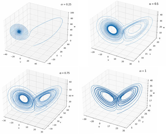
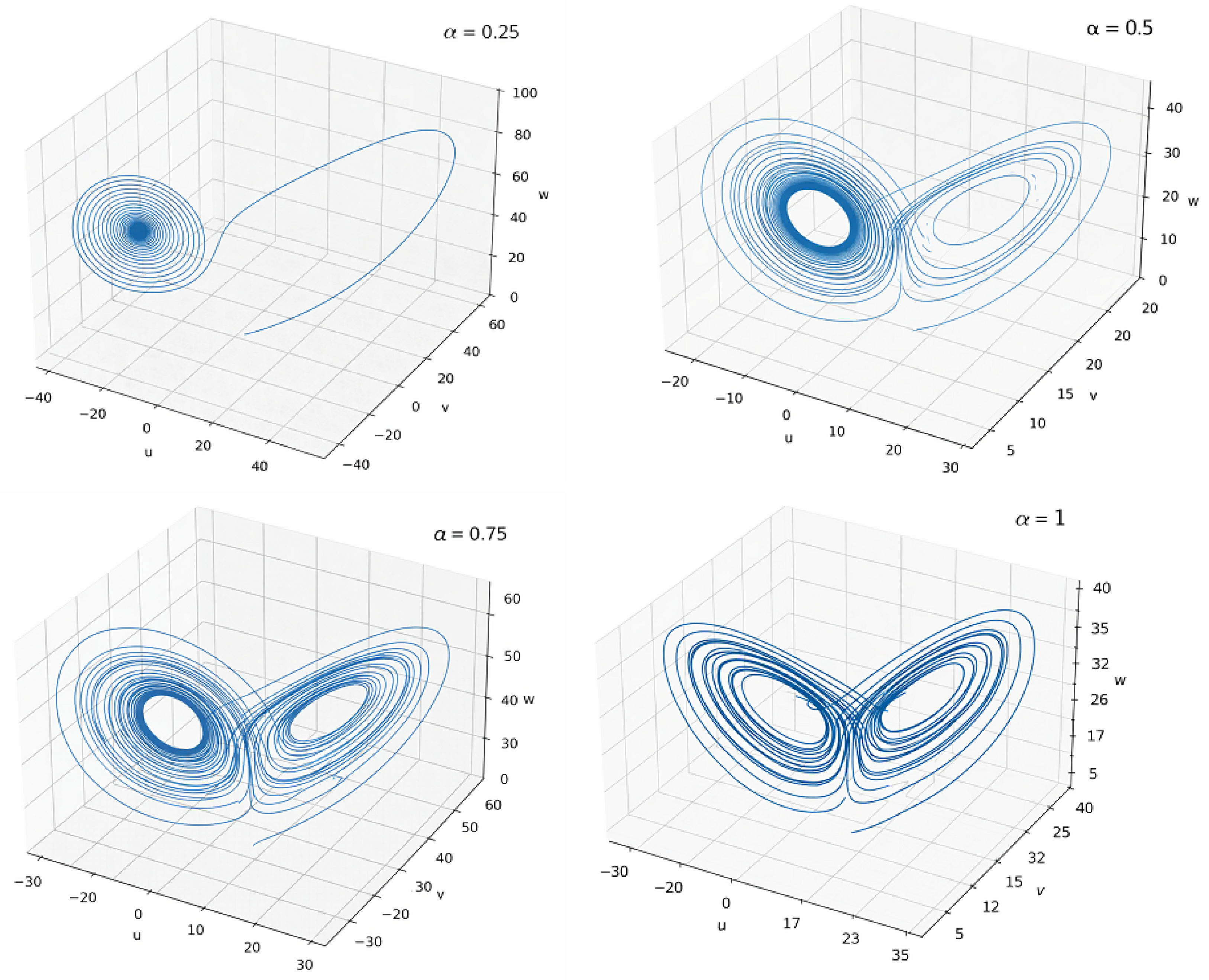
For example, if $\Omega$ is any closed interval in the system (29) with $\sigma =10$, $\rho =28$, $\beta ={\displaystyle \frac{8}{3}}$, $A^{\alpha }=1$ and with initial conditions $h_1=h_2=h_3=1$, then by using the expansion new iterative method [26], the solution is

$$\begin{array}{cc}\hfill u\left(t\right)& \approx 1+{\displaystyle \frac{260t^{2\alpha }}{\Gamma (2\alpha +1)}}+\cdots \hfill \end{array}$$

(31)

$$\begin{array}{cc}\hfill v\left(t\right)& \approx 1+{\displaystyle \frac{26t^{\alpha }}{\Gamma (\alpha +1)}}-{\displaystyle \frac{73}{3}}{\displaystyle \frac{t^{2\alpha }}{\Gamma (2\alpha +1)}}+\cdots \hfill \end{array}$$

(32)

$$\begin{array}{cc}\hfill w\left(t\right)& \approx 1-{\displaystyle \frac{5}{3}}{\displaystyle \frac{t^{\alpha }}{\Gamma (\alpha +1)}}+{\displaystyle \frac{274}{9}}{\displaystyle \frac{t^{2\alpha }}{\Gamma (2\alpha +1)}}+\cdots \hfill \end{array}$$

(33)

This solution is graphically presented in four cases, $\alpha =0.25$, $\alpha =0.5$, $\alpha =0.75$, and $\alpha =1$, see Figure 1. $\Omega$ is any closed interval.

Figure 1. Solution of (29) with $\sigma =10$, $\rho =28$, $\beta ={\displaystyle \frac{8}{3}}$, $A^{\alpha }=1$ and with initial conditions $h_1=h_2=h_3=1$.

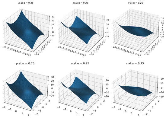
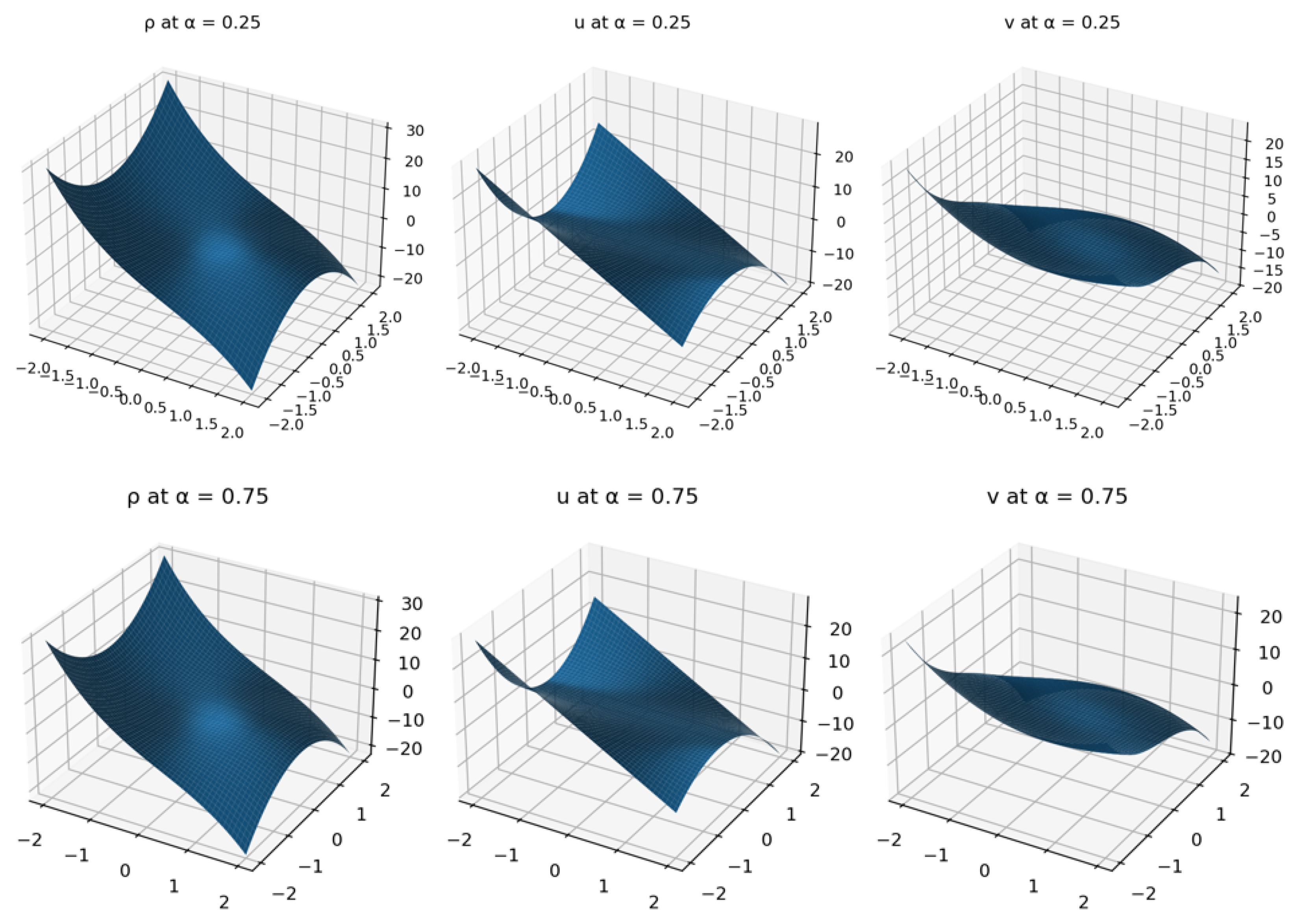
In the system (29), if $\Omega =[1,2]$ is a closed interval with $A^{\alpha }=1$, $\gamma =2$, and initial conditions $\rho (x,y,0)=x^2,u(x,y,0)=y^2,v(x,y,0)=xy,e(x,y,0)=xy$ in the system (30), then by using the expansion new iterative method, [26], the solution is

$$\begin{array}{cc}\hfill \rho (x,y,t)& \approx x^2-{\displaystyle \frac{\left(x^3+2x{y}^2\right)t^{\alpha }}{\Gamma (\alpha +1)}}+\cdots \hfill \end{array}$$

(34)

$$\begin{array}{cc}\hfill u(x,y,t)& \approx y^2-{\displaystyle \frac{\left(2x{y}^2+3y\right)t^{\alpha }}{\Gamma (\alpha +1)}}+\cdots \hfill \end{array}$$

(35)

$$\begin{array}{cc}\hfill v(x,y,t)& \approx xy-{\displaystyle \frac{\left(y^3+x^{2}y+x\right)t^{\alpha }}{\Gamma (\alpha +1)}}+\cdots \hfill \end{array}$$

(36)

$$\begin{array}{cc}\hfill E(x,y,t)& \approx x^{3}y+{\displaystyle \frac{1}{2}}{x}^2{y}^4+{\displaystyle \frac{1}{2}}{x}^4{y}^2-{\displaystyle \frac{\left(6x^2{y}^3+x{y}^6+\frac{9}{2}{x}^3{y}^4+4x^{4}y+\frac{3}{2}{x}^5{y}^2\right)t^{\alpha }}{\Gamma (\alpha +1)}}+\cdots \hfill \end{array}$$

(37)

This solution $\rho$, u, and v of (30) (with $A^{\alpha }=1$, $\gamma =2$, $t=1$) is graphically presented in two cases, $\alpha =0.25$ and $\alpha =0.75$, see Figure 2.

Figure 2. Solution $\rho$, u, and v of (30) with $A^{\alpha }=1$, $\gamma =2$, $t=1$ and with initial conditions $\rho (x,y,0)=x^2,u(x,y,0)=y^2,v(x,y,0)=xy,e(x,y,0)=xy$.

6. Conclusions

In this paper, we studied a two-dimensional ABC fractional dynamical system in a Banach space. Using fixed point theorems, we proved the existence and uniqueness of solutions and established Hyers–Ulam stability. We then applied our theoretical results to the fractional Lorenz system and the two-dimensional fractional Euler system. For the ABC fractional Lorenz model, the analysis was mainly based on time-dependent nonlinear terms with explicit Lipschitz constants. In contrast, the two-dimensional ABC fractional Euler system involved spatial derivatives and more complex nonlinear interactions. Despite these structural differences both models satisfied the required conditions, confirming the strength and flexibility of our abstract framework. Future research may extend this study to more general fractional operators and higher-dimensional systems. Numerical simulations and computational methods can also be developed to support the theoretical results. In addition, other nonlinear fractional models arising in physics and engineering may be analyzed using the same framework.

References

- Wang, M.; Din, M.; Zhou, M. Some fixed point results for novel contractions with applications in fractional differential equations for market equilibrium and economic growth. Fractal Fract. 2025, 9, 324. [Google Scholar] [CrossRef] [Scilit]
- Damag, F.H.; Saif, A.; Kiliçman, A. φ-Hilfer fractional Cauchy problems with almost sectorial and Lie bracket operators in Banach algebras. Fractal Fract. 2024, 8, 741. [Google Scholar] [CrossRef] [Scilit]
- Ashraf, R.; Nawaz, R.; Alabdali, O.; Fewster-Young, N.; Ali, A.H.; Ghanim, F.; Alb Lupas, A. A new hybrid optimal auxiliary function method for approximate solutions of nonlinear fractional PDEs. Fractal Fract. 2023, 7, 673. [Google Scholar] [CrossRef] [Scilit]
- Hamza, A.E.; Osman, O.; Ali, A.; Alsulami, A.; Aldwoah, K.; Mustafa, A.; Saber, H. Fractal-fractional modeling of liver fibrosis disease. Fractal Fract. 2024, 8, 638. [Google Scholar] [CrossRef] [Scilit]
- Adel, M.; Aldwoah, K.; Alahmadi, F.; Osman, M.S. The asymptotic behavior for a binary alloy in energy and material science: The unified method and its applications. J. Ocean Eng. Sci. 2024, 9, 373–378. [Google Scholar] [CrossRef] [Scilit]
- Li, Y.; Liu, F.; Turner, I.W.; Li, T. Time-fractional diffusion equation for signal smoothing. Appl. Math. Comput. 2018, 326, 108–116. [Google Scholar] [CrossRef] [Scilit]
- Aldwoah, K.A.; Almalahi, M.A.; Shah, K.; Awadalla, M.; Egami, R.H. Dynamics analysis of dengue fever model with harmonic mean type under fractal-fractional derivative. AIMS Math. 2024, 9, 13894–13926. [Google Scholar] [CrossRef] [Scilit]
- Campos, P.M.; Rodrigues, J.F. Unilateral problems for quasilinear operators with fractional Riesz gradients. Adv. Nonlinear Anal. 2025, 14, 20250084. [Google Scholar] [CrossRef] [Scilit]
- Liang, S.; Song, Y.; Shi, S. Concentrating solutions for double critical fractional Schrödinger–Poisson system with p-Laplacian in R3. Adv. Nonlinear Anal. 2025, 14, 20240063. [Google Scholar] [CrossRef] [Scilit]
- Arık, İ.A.; Araz, S.İ. Delay differential equations with fractional differential operators: Existence, uniqueness and applications to chaos. Commun. Anal. Mech. 2024, 16, 169–192. [Google Scholar] [CrossRef] [Scilit]
- Sun, L.; Wang, Z.; Wei, Y. A second–order approximation scheme for Caputo–Hadamard derivative and its application in fractional Allen–Cahn equation. Commun. Anal. Mech. 2025, 17, 630–661. [Google Scholar] [CrossRef] [Scilit]
- Balegh, M.; GhezaL, A. Theoretical analysis and applications of fixed-point theorems in delay fractional differential equations. J. Appl. Math. Comput. 2025, 71, 867–881. [Google Scholar] [CrossRef] [Scilit]
- Cona, L.; Kocağ, A.H. Fixed point approach for fractional order differential equation systems. J. New Results Sci. 2025, 14, 124–137. [Google Scholar] [CrossRef] [Scilit]
- Belhadj, M.; Roshan, J.R.; Radenović, S.S. Generalizations of Darbo’s fixed point theorem and its application to the solvability of a nonlinear fractional differential equation. Nonlinear Anal. Model. Control 2025, 30, 1081–1102. [Google Scholar] [CrossRef] [Scilit]
- Ahmad, H.; Din, F.U.; Younis, M. Fractional order Lorenz dynamics: Investigating existence and uniqueness via basic contraction. J. Appl. Math. Comput. 2025, 71, 6827–6858. [Google Scholar] [CrossRef] [Scilit]
- Awais, M.; Khan, M.A.; Bashir, Z. Exploring the stochastic patterns of hyperchaotic Lorenz systems with variable fractional order and radial basis function networks. Clust. Comput. 2024, 27, 9031–9064. [Google Scholar] [CrossRef] [Scilit]
- Meera, K.; Selvaganesan, N. Generalized fractional order complex Lorenz system based dual layer security enhancement approach. IEEE Access 2025, 13, 112162–112175. [Google Scholar] [CrossRef] [Scilit]
- Hui, W.H.; Li, P.Y.; Li, Z.W. A unified coordinate system for solving the two-dimensional Euler equations. J. Comput. Phys. 1999, 153, 596–637. [Google Scholar] [CrossRef] [Scilit]
- Chen, S. Stability of transonic shock fronts in two-dimensional Euler systems. Trans. Am. Math. Soc. 2005, 357, 287–308. [Google Scholar] [CrossRef] [Scilit]
- Wang, W.; Yang, T. Existence and stability of planar diffusion waves for 2-D Euler equations with damping. J. Differ. Equ. 2007, 242, 40–71. [Google Scholar] [CrossRef] [Scilit]
- Dullin, H.R.; Marangell, R.; Worthington, J. Instability of equilibria for the two-dimensional Euler equations on the torus. SIAM J. Appl. Math. 2016, 76, 1446–1470. [Google Scholar] [CrossRef] [Scilit]
- Alfwzan, W.; Yao, S.W.; Allehiany, F.M.; Ahmad, S.; Saifullah, S.; Inc, M. Fractional nonlinear tsunami shallow water model. Results Phys. 2023, 52, 106707. [Google Scholar] [CrossRef] [Scilit]
- Zeidler, E. Nonlinear Functional Analysis and Its Applications I: Fixed-Point Theorems; Springer: New York, NY, USA, 1986. [Google Scholar]
- Rudin, W. Principles of Mathematical Analysis, 3rd ed.; McGraw-Hill: New York, NY, USA, 1976. [Google Scholar]
- Rus, I.A. Ulam stabilities of ordinary differential equations in a Banach space. Carpath. J. Math. 2010, 26, 103–107. [Google Scholar]
- Damag, F.H.; Kiliçman, A.; Amin, R. Topological analysis with some techniques for solving a fractional tsunami shallow water mathematical model based on Hausdorff locally compact structures and their analytical implications. AIMS Math. 2026, 11, 3957–3985. [Google Scholar] [CrossRef] [Scilit]
Disclaimer/Publisher’s Note: The statements, opinions and data contained in all publications are solely those of the individual author(s) and contributor(s) and not of MDPI and/or the editor(s). MDPI and/or the editor(s) disclaim responsibility for any injury to people or property resulting from any ideas, methods, instructions or products referred to in the content. |
© 2026 by the authors. Licensee MDPI, Basel, Switzerland. This article is an open access article distributed under the terms and conditions of the Creative Commons Attribution (CC BY) license.