Control and Synchronization of Julia Sets of the Discrete Three-Dimensional Fractional HCV Model

Abstract

This paper investigates the fractal dynamical behavior of a discrete Caputo fractional-order hepatitis C virus model. First, we analyze the stability of the system by using spectral radius and design the fractional-order controller based on coordinate transformation. Then, a nonlinear coupling controller is constructed to achieve synchronization between two fractional-order models with different parameters and different fractional orders, and the synchronization is supported by rigorous mathematical proof. Numerical simulations are used to verify the effectiveness of control and synchronization.

1. Introduction

Hepatitis C virus (HCV) infection remains an important global public health problem. Although blood transfusion screening, the widespread use of disposable medical devices, and the application of direct-acting antivirals have reduced new infections to some extent in some regions, HCV transmission continues due to factors such as high-risk behaviors, disparities in access to treatment, and the accumulation of previous infections [1,2,3]. In infectious disease dynamics, the “Susceptible–Acute–Latent” compartmental structure is commonly used to describe disease processes with chronic characteristics, and key epidemiological patterns can be revealed through threshold and stability analyses [4]. On this basis, the existing studies have further introduced mechanisms such as treatment and recovery and combined them with population risk stratification to evaluate the integrated effects of interventions including screening and treatment [5,6,7]. In addition, in order to systematically characterize the transmission mechanisms of HCV, mathematical modeling has become an important research tool [8,9,10,11].

In addition to classical integer-order models, fractional-order dynamical systems have received widespread attention in infectious disease modeling in recent years. Fractional-order operators can introduce memory effects while maintaining a relatively simple model structure, thereby better capturing typical epidemiological features such as chronic disease transmission and intervention delays [12,13,14]. The most important advantage of fractional differential equations is that they include the characteristics of integer-order systems within fractional-order systems, and they can better simulate physical processes and dynamical systems. Moreover, various fractional integrals offer distinct advantages in theoretical analysis: sharp Hermite–Hadamard bounds are derived using Riemann–Liouville fractional integrals [15], the Grünwald–Letnikov fractional PID is used for enhanced adaptive cruise control [16], fractional integral inequalities are derived with the aid of the Atangana–Baleanu fractional integral operator [17], and the Caputo–Fabrizio fractional integral facilitates the establishment of Hermite–Hadamard-type inequalities for non-convex functions [18], thereby enriching the mathematical framework for fractional integrals. Meanwhile, discretization conforms to realistic data acquisition processes such as daily or stage-based sampling. Furthermore, with the introduction of fractional-order operators, fractional difference equations can further reflect complex nonlinear dynamical phenomena [19,20,21,22].

In the theory of dynamical systems, fractals can be described and studied from the perspective of mathematical methods to investigate complex phenomena. Julia sets reveal the fractal geometric characteristics of dynamical behaviors from a global perspective, and they have broad application fields, including the study of infectious diseases. Furthermore, the existing work has extended the research focus to the influence of stochastic perturbations and other factors on the geometric structures of Julia sets [23], as well as the control and synchronization of Julia sets [24,25,26], and has adopted control methods such as optimal function control [27], state feedback control [28], gradient control [27] and adaptive synchronization [29] to achieve the regulation and synchronization of fractal structures. In recent years, extensive studies have carried out on fractional-order fractal sets, and related results have indicated that variations in the fractional orders and system parameters affect the morphology and stability regions of fractal structures [30,31].

Based on the above research background, the main work of this paper is summarized as follows:

(i)

The research content of fractional-order fractal dynamical systems is enriched. From the perspective of fractal dynamics, the three-dimensional fractional-order HCV model is studied, high-dimensional systems exhibit more complex dynamical characteristics. Discrete-time modeling conforms to the fact that infectious disease data are obtained in discrete time and is therefore of greater practical significance, and the influence of the fractional orders on the system dynamics is analyzed.

(ii)

The scope of traditional fractal dynamics analysis is broadened. Based on the spectral radius of the Jacobian matrix at the fixed point, the stability of the system is analyzed. By using coordinate transformation, the controller for the three-dimensional fractional-order model is designed, and the range of the control parameter k is determined when the controlled model is stable, thereby realizing the control of the Julia set. This control method broadens the scope of traditional fractal dynamics analysis and can be applied to other fields.

(iii)

A rigorous proof of synchronization for two HCV models with different fractional orders is provided. A nonlinear coupling controller is constructed to realize the synchronization of Julia sets of two HCV models with different parameters and different fractional orders. This compensates for the deficiencies of related theoretical work and can serve as preparatory work for synchronization control of more complex fractional-order models in future research.

The remainder of this paper is organized as follows: Section 2 introduces the preliminary knowledge. Section 3 establishes a discrete fractional-order HCV model. Section 4 analyzes the stability of the model and discusses the control method for the Julia set of the HCV model. Section 5 proposes the synchronization method and provides its theoretical proof and numerical simulations. Section 6 concludes the paper.

2. Preliminaries

Consider a polynomial mapping $f:\mathbb{C}\to \mathbb{C}$ on the complex plane $\mathbb{C}$. According to references [30,32], the definition of the Julia set is as follows:

Definition 1.

The filled Julia set $K\left(f\right)$ of the mapping f is defined as the set of all points that remain bounded under the iteration of f.

$$K\left(f\right)=\left\{z\in \mathbb{C}\mid {\left\{f^k\left(z\right)\right\}}_{k=0}^{\infty }\mathit{is}\mathit{bounded}\right\}.$$

Correspondingly, the Julia set $J\left(f\right)$ is defined as the topological boundary of the filled Julia set.

$$J\left(f\right)=\partial K\left(f\right).$$

The Julia set $J\left(f\right)$ possesses basic topological properties such as being non-empty, bounded, and completely invariant, $f\left(J\left(f\right)\right)=J\left(f\right)=f^{-1}\left(J\left(f\right)\right)$.

Definition 2

([19]). Let function $u:{\mathbb{N}}_a\to \mathbb{R}$ and $\nu >0$, then the fractional sum of order ν is defined as follows:

$${\Delta }_a^{-\nu }u\left(t\right):={\displaystyle \frac{1}{\Gamma \left(\nu \right)}}\sum _{s=a}^{t-\nu }{(t-\delta \left(s\right))}^{(\nu -1)}u\left(s\right),t\in {\mathbb{N}}_{a+\nu },$$

where a is the starting point, $\delta \left(s\right)=s+1$, ${\mathbb{N}}_a=\{a,a+1,\dots \}$, and ${\mathbb{N}}_{a+\nu }=\{a+\nu ,a+\nu +1,\dots \}$. Furthermore, $t^{\left(\nu \right)}$ is defined by

$$t^{\left(\nu \right)}={\displaystyle \frac{\Gamma (t+1)}{\Gamma (t+1-\nu )}}.$$

Definition 3

([20]). For $\nu >0(\nu \notin \mathbb{N})$, and a function $u\left(t\right)$ defined on ${\mathbb{N}}_a$, the Caputo difference is defined by

$${}^C\Delta _a^{\nu }u\left(t\right):={\Delta }_a^{-(m-\nu )}{\Delta }^{m}u\left(t\right)={\displaystyle \frac{1}{\Gamma (m-\nu )}}\sum _{s=a}^{t-(m-\nu )}{(t-\delta \left(s\right))}^{(m-\nu -1)}{\Delta }_s^{m}u\left(s\right),$$

where ${\mathbb{N}}_a=\{a,a+1,\dots \}$, $t\in {\mathbb{N}}_{a+m-\nu }$, and $m=\left[\nu \right]+1$.

Lemma 1

([33]). For the initial value problem of the Caputo fractional difference equation

$$\left\{\begin{array}{cc}\hfill {}^C\Delta _a^{\nu }u\left(t\right)& =f(t+\nu -1,u(t+\nu -1\left)\right),\hfill \\ \hfill {\Delta }^{k}u\left(a\right)& =u_k,m=\left[\nu \right]+1,k=0,\dots ,m-1,\hfill \end{array}\right.$$

the equivalent summation Equation (discrete integral equation) is shown as follows:

$$u\left(t\right)=u_0\left(t\right)+{\displaystyle \frac{1}{\Gamma \left(\nu \right)}}\sum _{s=a+m-\nu }^{t-\nu }{(t-\delta \left(s\right))}^{(\nu -1)}f(s+\nu -1,u(s+\nu -1)),$$

(1)

where $t\in {\mathbb{N}}_{a+m}$, and the initial iteration $u_0\left(t\right)$ is

$$u_0\left(t\right)=\sum _{k=0}^{m-1}{\displaystyle \frac{{(t-a)}^{\left(k\right)}}{k!}}{\Delta }^{k}u\left(a\right).$$

The fractional-order operator has significant non-local characteristics, and its scope of action covers the entire domain, thereby affecting the overall behavior of the system. This characteristic enables the fractional-order model to effectively characterize the memory effects and historical cumulative influences of the system. By adjusting the fractional order, the memory length can be controlled, thereby more accurately describing the dynamic behavior of the system.

3. Fractional HCV Model

Based on the three-dimensional HCV dynamical system proposed in [12], and following [34], the total population is normalized and assumed to be 1, so that the equation is expressed in the following normalized form. Consequently, a dynamic model containing the mutual transformation relationships among susceptible individuals $S\left(t\right)$, acute infected individuals $A\left(t\right)$, and latent infected individuals $L\left(t\right)$ is constructed.

The integer-order HCV system is written as

$$\left\{\begin{array}{cc}\hfill {\displaystyle \frac{\mathrm{d}S}{\mathrm{d}t}}& =B_0-{\beta }_{0}S(A+L)+c_{r}A-{\mu }_{0}S,\hfill \\ \hfill {\displaystyle \frac{\mathrm{d}A}{\mathrm{d}t}}& ={\beta }_{0}S(A+L)-(c_r+{\theta }_0+{\mu }_0)A,\hfill \\ \hfill {\displaystyle \frac{\mathrm{d}L}{\mathrm{d}t}}& ={\theta }_{0}A-{\mu }_{0}L,\hfill \end{array}\right.$$

(2)

where $B_0$ is the natural birth rate, ${\beta }_0$ is the transmission parameter, $c_r$ represents the rate of spontaneous removal, ${\theta }_0$ is the rate of transition from the acute to latent stage, and ${\mu }_0$ is the natural removal rate.

Discrete models are more consistent with stage-wise sampled epidemiological data, so we discretize the continuous-time system (2), referring to [24], and use

$${\displaystyle \frac{\mathrm{d}X}{\mathrm{d}t}}⟶{\displaystyle \frac{X(t+\Delta t)-X\left(t\right)}{\Delta t}},X\in \{S,A,L\}.$$

(3)

Substitute (3) into (2) and take $B=\Delta t{B}_0$, $\beta =\Delta t{\beta }_0$, $c=\Delta t{c}_r$, $\mu =\Delta t{\mu }_0$, $\theta =\Delta t{\theta }_0$, then the following difference form is obtained,

$$\left\{\begin{array}{cc}\hfill S_{n+1}-S_n& =B-\beta S_n(A_n+L_n)+c{A}_n-\mu S_n,\hfill \\ \hfill A_{n+1}-A_n& =\beta S_n(A_n+L_n)-(c+\theta +\mu )A_n,\hfill \\ \hfill L_{n+1}-L_n& =\theta A_n-\mu L_n.\hfill \end{array}\right.$$

(4)

The Equation (4) can be rewritten as

$$\left\{\begin{array}{cc}\hfill \nabla S_{n+1}& =B-\beta S_n(A_n+L_n)+c{A}_n-\mu S_n,\hfill \\ \hfill \nabla A_{n+1}& =\beta S_n(A_n+L_n)-(c+\theta +\mu )A_n,\hfill \\ \hfill \nabla L_{n+1}& =\theta A_n-\mu L_n.\hfill \end{array}\right.$$

(5)

Fractional-order operators exhibit memory effects in biological systems, among various fractional-order definitions, the Caputo-type operator is suitable for infectious disease modeling [12]. On this basis, according to Definition 3 and Lemma 1, the corresponding integer-order Equation (5) is then extended to its fractional-order form,

$$\left\{\begin{array}{cc}\hfill {}^C\Delta _a^{\alpha }S\left(t\right)& =B-\beta S(t+\alpha -1)\left(A\right(t+\alpha -1)+L(t+\alpha -1\left)\right)\hfill \\ \hfill & +cA(t+\alpha -1)-\mu S(t+\alpha -1),\hfill \\ \hfill {}^C\Delta _a^{\alpha }A\left(t\right)& =\beta S(t+\alpha -1)\left(A\right(t+\alpha -1)+L(t+\alpha -1\left)\right)\hfill \\ \hfill & -(c+\theta +\mu )A(t+\alpha -1),\hfill \\ \hfill {}^C\Delta _a^{\alpha }L\left(t\right)& =\theta A(t+\alpha -1)-\mu L(t+\alpha -1).\hfill \end{array}\right.$$

(6)

According to Lemma 1, system (6) can be transformed into the following discrete integral form, where $\alpha \in (0,1]$, $m=\left[\alpha \right]+1$, $t\in {\mathbb{N}}_{a+1}$, ${\mathbb{N}}_{a+1}=a+1,a+2,\dots$,

$$\left\{\begin{array}{cc}\hfill S\left(t\right)=S\left(a\right)& +{\displaystyle \frac{1}{\Gamma \left(\alpha \right)}}\sum _{s=1+a-\alpha }^{t-\alpha }{\displaystyle \frac{\Gamma (t-s)}{\Gamma (t-s+1-\alpha )}}[B-\beta S(s+\alpha -1)(A(s+\alpha -1)+L(s+\alpha -1))\hfill \\ \hfill & +cA(s+\alpha -1)-\mu S(s+\alpha -1)],\hfill \\ \hfill A\left(t\right)=A\left(a\right)& +{\displaystyle \frac{1}{\Gamma \left(\alpha \right)}}\sum _{s=1+a-\alpha }^{t-\alpha }{\displaystyle \frac{\Gamma (t-s)}{\Gamma (t-s+1-\alpha )}}[\beta S(s+\alpha -1)(A(s+\alpha -1)+L(s+\alpha -1))\hfill \\ \hfill & -(c+\theta +\mu )A(s+\alpha -1)],\hfill \\ \hfill L\left(t\right)=L\left(a\right)& +{\displaystyle \frac{1}{\Gamma \left(\alpha \right)}}\sum _{s=1+a-\alpha }^{t-\alpha }{\displaystyle \frac{\Gamma (t-s)}{\Gamma (t-s+1-\alpha )}}[\theta A(s+\alpha -1)-\mu L(s+\alpha -1)].\hfill \end{array}\right.$$

(7)

Consequently, the numerical equation can be gained,

$$\left\{\begin{array}{cc}\hfill S\left(n\right)=S\left(a\right)& +{\displaystyle \frac{1}{\Gamma \left(\alpha \right)}}\sum _{j=a+1}^n{\displaystyle \frac{\Gamma (n-j+\alpha )}{\Gamma (n-j+1)}}[B-\beta S(j-1)(A(j-1)+L(j-1))\hfill \\ & +cA(j-1)-\mu S(j-1)],\hfill \\ \hfill A\left(n\right)=A\left(a\right)& +{\displaystyle \frac{1}{\Gamma \left(\alpha \right)}}\sum _{j=a+1}^n{\displaystyle \frac{\Gamma (n-j+\alpha )}{\Gamma (n-j+1)}}[\beta S(j-1)(A(j-1)+L(j-1))\hfill \\ & -(c+\theta +\mu )A(j-1)],\hfill \\ \hfill L\left(n\right)=L\left(a\right)& +{\displaystyle \frac{1}{\Gamma \left(\alpha \right)}}\sum _{j=a+1}^n{\displaystyle \frac{\Gamma (n-j+\alpha )}{\Gamma (n-j+1)}}[\theta A(j-1)-\mu L(j-1)].\hfill \end{array}\right.$$

(8)

Referring to [35], take $a=0$, since a is the starting point of the accumulation of the discrete fractional sum, set the initial value of the equation at this starting point, and the summation starts with $j=1$, the model can be written as

$$\left\{\begin{array}{cc}\hfill S\left(n\right)=S\left(0\right)& +{\displaystyle \frac{1}{\Gamma \left(\alpha \right)}}\sum _{j=1}^n{\displaystyle \frac{\Gamma (n-j+\alpha )}{\Gamma (n-j+1)}}[B-\beta S(j-1)(A(j-1)+L(j-1))+cA(j-1)-\mu S(j-1)],\hfill \\ \hfill A\left(n\right)=A\left(0\right)& +{\displaystyle \frac{1}{\Gamma \left(\alpha \right)}}\sum _{j=1}^n{\displaystyle \frac{\Gamma (n-j+\alpha )}{\Gamma (n-j+1)}}[\beta S(j-1)(A(j-1)+L(j-1))-(c+\theta +\mu )A(j-1)],\hfill \\ \hfill L\left(n\right)=L\left(0\right)& +{\displaystyle \frac{1}{\Gamma \left(\alpha \right)}}\sum _{j=1}^n{\displaystyle \frac{\Gamma (n-j+\alpha )}{\Gamma (n-j+1)}}[\theta A(j-1)-\mu L(j-1)].\hfill \end{array}\right.$$

(9)

From Equation (9), it can be seen that the current state $X\left(n\right)\in \left\{S\right(n),A(n),L(n\left)\right\}$ depends on all historical states $X\left(0\right),\dots ,X(n-1)$, and the fractional kernel function ${\displaystyle \frac{\Gamma (n-j+\alpha )}{\Gamma (n-j+1)}}$ reflects the long-term memory characteristic of the fractional-order system. Based on Definition 1, if $X\left(n\right)$ remains bounded in the sense of iteration, the corresponding initial value points belong to the filled Julia set of the three-dimensional discrete HCV system (9), and its boundary is called the Julia set of the system (9).

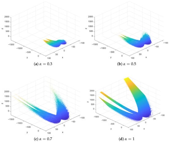
To intuitively demonstrate the influence of the fractional order on the dynamic behavior of the system, the escape time algorithm is employed to plot the Julia set while keeping the window size unchanged. The simulation parameters are set as follows: escape radius $R={10}^5$ and maximum iteration steps $\mathrm{st}=100$. Additionally, the discrete grid boundaries are uniformly set to $x\in [-110,100]$, $y\in [-1800,300]$, and $z\in [-350,2000]$, with a grid resolution of 500. Unlike the cholera modeling study [36], where real epidemiological data are used for parameter estimation and for RMSE-based comparisons between the integer-order and fractional-order models, our work focuses primarily on the fractal dynamics and Julia-set structure of the fractional HCV system. The transmission parameter $\beta$, the natural removal rate $\mu$, and the rate of transition from acute to latent stage $\theta$, the rate of spontaneous removal c are taken to be the same as in reference [12], these numerical values represent the proportion of individuals undergoing state transitions per unit time, and B is scaled from reference data to unify the units and then fine-tuned through empirical observation, set $B=0.0221$, $\beta =0.05$, $\mu =0.0158$, $\theta =1$, and $c=0.27$. In addition, fractional orders $\alpha =0.3,0.5,0.7,1$ are considered, then the filled Julia sets of system (9) is shown in Figure 1. The cool blue points represent low values, while the warm yellow points represent high values.

Figure 1. Filled Julia sets of system (9) with different fractional orders $\alpha$.

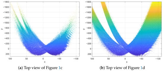
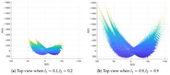
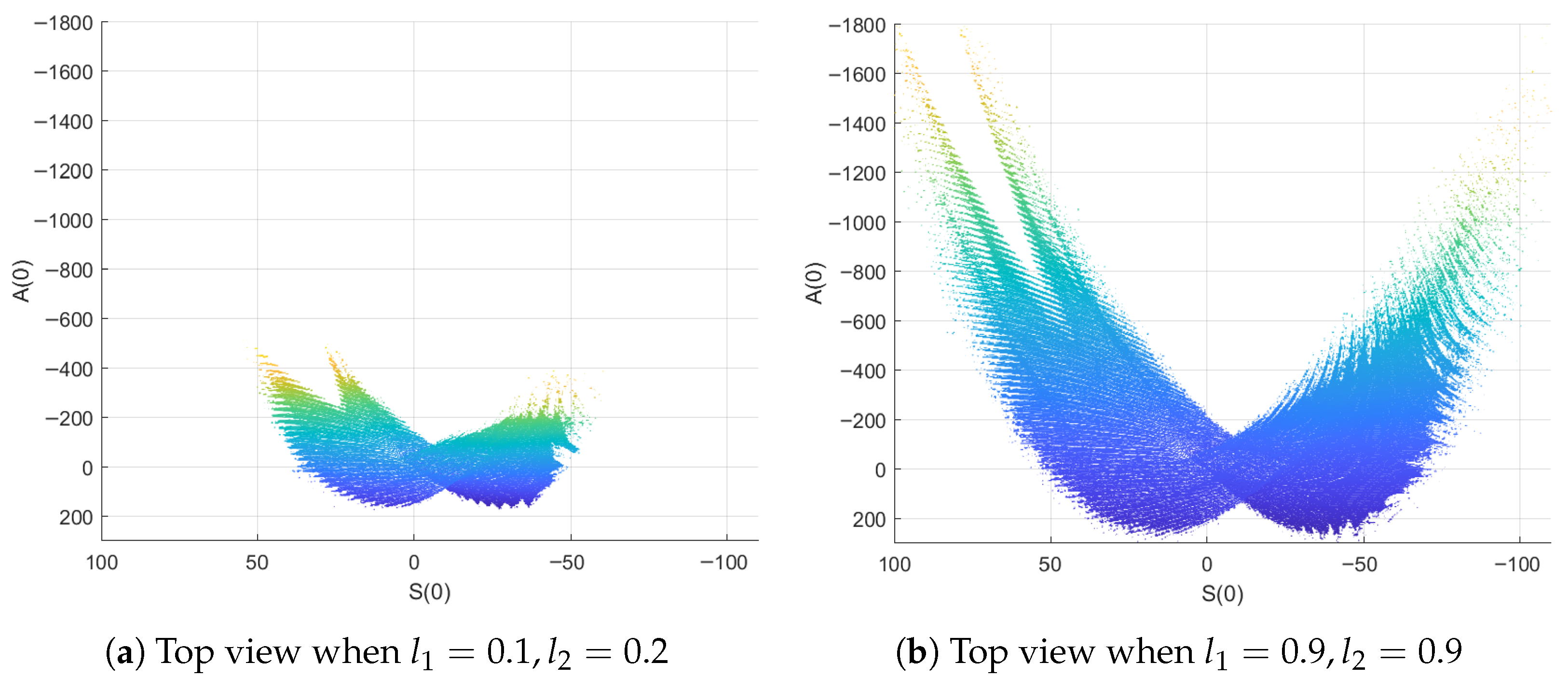
From Figure 1 and Figure 2, it can be observed that the Julia set of the HCV model presents a butterfly shape. As the fractional order $\alpha$ increases, the shape of the butterfly’s two wings also becomes significantly larger, and when $\alpha$ varies from $0.7$ to 1, the inner gap within the left wing becomes progressively deeper and extends inward. These observations indicate that the fractional-order memory effects have a profound impact on the dynamic behavior of the HCV system and also confirm the necessity of introducing fractional orders to study the model. When $\alpha =1$, the fractional-order HCV model degenerates into the corresponding integer-order one.

Figure 2. Top view of filled Julia sets of system (9) when fractional order $\alpha =0.7$ and $\alpha =1$.

4. Control of Julia Sets

First, with the aid of coordinate transformation, let the memory length be a fixed positive integer N, satisfying $(N<n)$. We transform the three-dimensional system (9) into an equivalent multi-dimensional system.

$$\begin{array}{cc}\hfill z_i\left(n\right)& =S(n+i-N),i\in \{1,2,3,\dots ,N\},\hfill \\ \hfill z_i\left(n\right)& =A(n+i-2N),i\in \{N+1,N+2,\dots ,2N\},\hfill \\ \hfill z_i\left(n\right)& =L(n+i-3N),i\in \{2N+1,2N+2,\dots ,3N\}.\hfill \end{array}$$

We can obtain $z_1(n+1)=S(n+2-N)=z_2\left(n\right),\dots ,z_{N-1}(n+1)=S\left(n\right)=z_N\left(n\right)$.

$$\begin{array}{ccc}\hfill z_N(n+1)& =S(n+1)\hfill & \\ & =S\left(0\right)+{\displaystyle \frac{1}{\Gamma \left(\alpha \right)}}\sum _{j=1}^{n+1}{\displaystyle \frac{\Gamma (n+1-j+\alpha )}{\Gamma (n+2-j)}}[B-\beta S(j-1)(A(j-1)+L(j-1))\hfill & \\ & +cA(j-1)-\mu S(j-1)].\hfill \end{array}$$

Similarly, we obtain $z_{N+1}(n+1)=A(n+2-N)=z_{N+2}\left(n\right),\dots ,z_{2N-1}(n+1)=A\left(n\right)=z_{2N}\left(n\right)$,

$$\begin{array}{ccc}\hfill z_{2N}(n+1)& =A(n+1)\hfill & \\ & =A\left(0\right)+{\displaystyle \frac{1}{\Gamma \left(\alpha \right)}}\sum _{j=1}^{n+1}{\displaystyle \frac{\Gamma (n+1-j+\alpha )}{\Gamma (n+2-j)}}[\beta S(j-1)(A(j-1)+L(j-1))\hfill & \\ & -(c+\theta +\mu )A(j-1)],\hfill \end{array}$$

and $z_{2N+1}(n+1)=L(n+2-N)=z_{2N+2}\left(n\right),\dots ,z_{3N-1}(n+1)=L\left(n\right)=z_{3N}\left(n\right)$,

$$\begin{array}{ccc}\hfill z_{3N}(n+1)& =L(n+1)\hfill & \\ & =L\left(0\right)+{\displaystyle \frac{1}{\Gamma \left(\alpha \right)}}\sum _{j=1}^{n+1}{\displaystyle \frac{\Gamma (n+1-j+\alpha )}{\Gamma (n+2-j)}}[\theta A(j-1)-\mu L(j-1)].\hfill \end{array}$$

From ${\displaystyle \frac{1}{\Gamma \left(\alpha \right)}}{\displaystyle \frac{\Gamma (n+1-j+\alpha )}{\Gamma (n+2-j)}}=\left({\displaystyle \genfrac{}{}{0pt}{}{n+\alpha -j}{n+1-j}}\right)$, we can obtain

$$\begin{array}{ccc}\hfill z_N(n+1)& =S(n+1)\hfill & \\ & =S\left(0\right)+\sum _{j=1}^{n+1}\left({\displaystyle \genfrac{}{}{0pt}{}{n+\alpha -j}{n+1-j}}\right)[B-\beta S(j-1)(A(j-1)+L(j-1))\hfill & \\ & +cA(j-1)-\mu S(j-1)]\hfill & \\ & =S\left(0\right)+\sum _{j=1}^{n+1-N}\left({\displaystyle \genfrac{}{}{0pt}{}{n+\alpha -j}{n+1-j}}\right)[B-\beta S(j-1)(A(j-1)+L(j-1))\hfill & \\ & +cA(j-1)-\mu S(j-1)]+\sum _{j=n+2-N}^{n+1}\left({\displaystyle \genfrac{}{}{0pt}{}{n+\alpha -j}{n+1-j}}\right)[B-\beta S(j-1)\hfill & \\ & \times \left(A\right(j-1)+L(j-1\left)\right)+cA(j-1)-\mu S(j-1)]\hfill & \\ & =S\left(0\right)+\sum _{j=1}^{n+1-N}\left({\displaystyle \genfrac{}{}{0pt}{}{n+\alpha -j}{n+1-j}}\right)[B-\beta S(j-1)(A(j-1)+L(j-1))\hfill & \\ & +cA(j-1)-\mu S(j-1)]+\sum _{j=1}^N\left({\displaystyle \genfrac{}{}{0pt}{}{N-j+\alpha -1}{N-j}}\right)[B-\beta z_j\left(n\right)\hfill & \\ & \times (z_{j+N}\left(n\right)+z_{j+2N}\left(n\right))+c{z}_{j+N}\left(n\right)-\mu z_j\left(n\right)].\hfill \end{array}$$

Correspondingly,

$$\begin{array}{ccc}\hfill z_{2N}(n+1)& =A(n+1)\hfill & \\ & =A\left(0\right)+\sum _{j=1}^{n+1-N}\left({\displaystyle \genfrac{}{}{0pt}{}{n+\alpha -j}{n+1-j}}\right)[\beta S(j-1)(A(j-1)+L(j-1))\hfill & \\ & -(c+\theta +\mu )A(j-1)]+\sum _{j=1}^N\left({\displaystyle \genfrac{}{}{0pt}{}{N-j+\alpha -1}{N-j}}\right)\left[\beta z_j\left(n\right)\right(z_{j+N}\left(n\right)\hfill & \\ & +z_{j+2N}\left(n\right))-(c+\theta +\mu )z_{j+N}\left(n\right)],\hfill & \\ \hfill z_{3N}(n+1)& =L(n+1)\hfill & \\ & =L\left(0\right)+\sum _{j=1}^{n+1-N}\left({\displaystyle \genfrac{}{}{0pt}{}{n+\alpha -j}{n+1-j}}\right)[\theta A(j-1)-\mu L(j-1)]\hfill & \\ & +\sum _{j=1}^N\left({\displaystyle \genfrac{}{}{0pt}{}{N-j+\alpha -1}{N-j}}\right)[\theta z_{j+N}\left(n\right)-\mu z_{j+2N}\left(n\right)].\hfill \end{array}$$

Therefore, system (9) is transformed into the equivalent system

$$\left(\begin{array}{c}{z}_1(n+1)\\ ⋮\\ z_N(n+1)\\ z_{N+1}(n+1)\\ ⋮\\ z_{2N}(n+1)\\ z_{2N+1}(n+1)\\ ⋮\\ z_{3N}(n+1)\end{array}\right)=\left(\begin{array}{c}{z}_2\left(n\right)\\ ⋮\\ h_1^{*}(S\left(0\right),\dots ,S(n-N),z_1\left(n\right),\dots ,z_{3N}\left(n\right))\\ z_{N+2}\left(n\right)\\ ⋮\\ h_2^{*}(A\left(0\right),\dots ,A(n-N),z_1\left(n\right),\dots ,z_{3N}\left(n\right))\\ z_{2N+2}\left(n\right)\\ ⋮\\ h_3^{*}(L\left(0\right),\dots ,L(n-N),z_1\left(n\right),\dots ,z_{3N}\left(n\right))\end{array}\right),$$

(10)

where

$$\begin{array}{ccc}\hfill h_1^{*}(·)& =S\left(0\right)+\sum _{j=1}^{n+1-N}\left({\displaystyle \genfrac{}{}{0pt}{}{n+\alpha -j}{n+1-j}}\right)[B-\beta S(j-1)(A(j-1)+L(j-1))+cA(j-1)\hfill & \\ & -\mu S(j-1)]+\sum _{j=1}^N\left({\displaystyle \genfrac{}{}{0pt}{}{N-j+\alpha -1}{N-j}}\right)[B-\beta z_j\left(n\right)(z_{j+N}\left(n\right)+z_{j+2N}\left(n\right))\hfill & \\ & +c{z}_{j+N}\left(n\right)-\mu z_j\left(n\right)],\hfill & \\ \hfill h_2^{*}(·)& =A\left(0\right)+\sum _{j=1}^{n+1-N}\left({\displaystyle \genfrac{}{}{0pt}{}{n+\alpha -j}{n+1-j}}\right)[\beta S(j-1)(A(j-1)+L(j-1))\hfill & \\ & -(c+\theta +\mu )A(j-1)]+\sum _{j=1}^N\left({\displaystyle \genfrac{}{}{0pt}{}{N-j+\alpha -1}{N-j}}\right)[\beta z_j\left(n\right)(z_{j+N}\left(n\right)+z_{j+2N}\left(n\right))\hfill & \\ & -(c+\theta +\mu )z_{j+N}\left(n\right)],\hfill & \\ \hfill h_3^{*}(·)& =L\left(0\right)+\sum _{j=1}^{n+1-N}\left({\displaystyle \genfrac{}{}{0pt}{}{n+\alpha -j}{n+1-j}}\right)[\theta A(j-1)-\mu L(j-1)]\hfill & \\ & +\sum _{j=1}^N\left({\displaystyle \genfrac{}{}{0pt}{}{N-j+\alpha -1}{N-j}}\right)[\theta z_{j+N}\left(n\right)-\mu z_{j+2N}\left(n\right)].\hfill \end{array}$$

To control the system (9), we aim to design a controller about the fixed point, so we first need to determine the fixed point. Let $(S^{*},A^{*},L^{*})$ be the fixed point of system (9), then we have

$$\left\{\begin{array}{cc}\hfill S^{*}& =S^{*}+{\displaystyle \frac{1}{\Gamma \left(\alpha \right)}}\sum _{j=1}^n{\displaystyle \frac{\Gamma (n-j+\alpha )}{\Gamma (n-j+1)}}[B-\beta S^{*}(A^{*}+L^{*})+c{A}^{*}-\mu S^{*}],\hfill \\ \hfill A^{*}& =A^{*}+{\displaystyle \frac{1}{\Gamma \left(\alpha \right)}}\sum _{j=1}^n{\displaystyle \frac{\Gamma (n-j+\alpha )}{\Gamma (n-j+1)}}[\beta S^{*}(A^{*}+L^{*})-(c+\theta +\mu )A^{*}],\hfill \\ \hfill L^{*}& =L^{*}+{\displaystyle \frac{1}{\Gamma \left(\alpha \right)}}\sum _{j=1}^n{\displaystyle \frac{\Gamma (n-j+\alpha )}{\Gamma (n-j+1)}}[\theta A^{*}-\mu L^{*}].\hfill \end{array}\right.$$

Following the same simplification procedure in [37], one has the identity

$${\displaystyle \frac{1}{\Gamma \left(\alpha \right)}}\sum _{j=1}^n{\displaystyle \frac{\Gamma (n-j+\alpha )}{\Gamma (n-j+1)}}={\displaystyle \frac{\Gamma (n+\alpha )}{\Gamma \left(n\right)\Gamma (\alpha +1)}},$$

therefore, the fixed point equation can be equivalently rewritten as

$$\left\{\begin{array}{cc}\hfill S^{*}& =S^{*}+{\displaystyle \frac{\Gamma (n+\alpha )}{\Gamma \left(n\right)\Gamma (\alpha +1)}}[B-\beta S^{*}(A^{*}+L^{*})+c{A}^{*}-\mu S^{*}],\hfill \\ \hfill A^{*}& =A^{*}+{\displaystyle \frac{\Gamma (n+\alpha )}{\Gamma \left(n\right)\Gamma (\alpha +1)}}[\beta S^{*}(A^{*}+L^{*})-(c+\theta +\mu )A^{*}],\hfill \\ \hfill L^{*}& =L^{*}+{\displaystyle \frac{\Gamma (n+\alpha )}{\Gamma \left(n\right)\Gamma (\alpha +1)}}[\theta A^{*}-\mu L^{*}].\hfill \end{array}\right.$$

(11)

To solve the above equation, it is equivalent to solve

$$\left\{\begin{array}{c}B-\beta S^{*}(A^{*}+L^{*})+c{A}^{*}-\mu S^{*}=0,\hfill \\ \beta S^{*}(A^{*}+L^{*})-(c+\theta +\mu )A^{*}=0,\hfill \\ \theta A^{*}-\mu L^{*}=0.\hfill \end{array}\right.$$

This yields two types of fixed points $(S^{*},A^{*},L^{*})$:

(i)

Disease-free fixed point $(S_1,A_1,L_1)=({\displaystyle \frac{B}{\mu }},0,0)$,

(ii)

Coexistence fixed point $S_2={\displaystyle \frac{c+\theta +\mu }{\beta (1+\theta /\mu )}},A_2={\displaystyle \frac{B-\mu S_2}{\theta +\mu }},L_2={\displaystyle \frac{\theta }{\mu }}{A}_2$.

Take parameters $B,\beta ,c,\theta ,\mu >0$. For the disease-free fixed point, $S_1>0,A_1=L_1=0$, only susceptible individuals are present in the population, which is a very ideal situation representing the absence of disease. Furthermore, for the coexistence fixed point, under the condition $B>\mu S_2$, which is $B>{\displaystyle \frac{{\mu }^2(c+\theta +\mu )}{\beta (\mu +\theta )}}$, then $S_2,A_2,L_2>0$. The common phenomenon is that susceptible, acute infected, latent infected coexist, and they can coexist for a long time and neither of them will suddenly go to zero. Therefore, the subsequent analysis focuses on the coexistence fixed point $(S^{*},A^{*},L^{*})=(S_2,A_2,L_2)$.

Theorem 1.

If the spectral radius $\rho \left(J\right)$ of the Jacobian matrix J of system (9) at the fixed point $(S^{*},A^{*},L^{*})$ satisfies

$$\rho \left(J\right)<1,$$

then system (9) is locally asymptotically stable at the fixed point $(S^{*},A^{*},L^{*})$.

Proof. 

According to the Hartman–Grobman Theorem [38,39], when the spectral radius $\rho \left(J\right)<1$ of the Jacobian matrix J, the linearized system of system (9) at the fixed point $(S^{*},A^{*},L^{*})$ is stable, and the dynamic behavior of the nonlinear system in the neighborhood of this fixed point is topologically equivalent to its linearized system; therefore, system (9) is locally asymptotically stable at the fixed point $(S^{*},A^{*},L^{*})$. □

Noting that system (9) is equivalent to system (10), from Theorem 1, it is known that the control of the Julia set of system (9) can be achieved by adding a controller on the Julia set of system (10) at the fixed point $F_e=(S^{*},\dots ,S^{*},A^{*},\dots ,A^{*},L^{*},\dots ,L^{*})$ ($3N$ dimensions). The Jacobian matrix of the right-hand function of system (10) at the fixed point $F_e$ is

$$J=\left(\begin{array}{cccccccccccc}0& 1& \dots & 0& 0& 0& \dots & 0& 0& 0& \dots & 0\\ 0& 0& \ddots & 0& 0& 0& \dots & 0& 0& 0& \dots & 0\\ ⋮& ⋮& \ddots & 1& ⋮& ⋮& \dots & 0& ⋮& ⋮& \dots & 0\\ f_1& f_2& \dots & f_N& f_1^{\prime }& f_2^{\prime }& \dots & f_N^{\prime }& f_1^{″}& f_2^{″}& \dots & f_N^{″}\\ 0& 0& \dots & 0& 0& 1& \dots & 0& 0& 0& \dots & 0\\ 0& 0& \dots & 0& 0& 0& \ddots & 0& 0& 0& \dots & 0\\ 0& \dots & 0& 0& 0& \dots & 0& 1& 0& \dots & 0& 0\\ g_1& g_2& \dots & g_N& g_1^{\prime }& g_2^{\prime }& \dots & g_N^{\prime }& g_1^{″}& g_2^{″}& \dots & g_N^{″}\\ ⋮& ⋮& ⋮& ⋮& ⋮& ⋮& ⋮& ⋮& 0& 1& \dots & 0\\ 0& \dots & 0& 0& 0& \dots & 0& 0& 0& 0& \ddots & 1\\ p_1& p_2& \dots & p_N& p_1^{\prime }& p_2^{\prime }& \dots & p_N^{\prime }& p_1^{″}& p_2^{″}& \dots & p_N^{″}\end{array}\right),$$

where

$$\begin{array}{cccc}\hfill f_j& =\left({\displaystyle \genfrac{}{}{0pt}{}{N-j+\alpha -1}{N-j}}\right)[-\beta (A^{*}+L^{*})-\mu ];\hfill & \hfill f_j^{\prime }& =\left({\displaystyle \genfrac{}{}{0pt}{}{N-j+\alpha -1}{N-j}}\right)(-\beta S^{*}+c);\hfill \\ \hfill f_j^{″}& =\left({\displaystyle \genfrac{}{}{0pt}{}{N-j+\alpha -1}{N-j}}\right)(-\beta S^{*});\hfill & \hfill g_j& =\left({\displaystyle \genfrac{}{}{0pt}{}{N-j+\alpha -1}{N-j}}\right)\left[\beta (A^{*}+L^{*})\right];\hfill \\ \hfill g_j^{\prime }& =\left({\displaystyle \genfrac{}{}{0pt}{}{N-j+\alpha -1}{N-j}}\right)[\beta S^{*}-(c+\theta +\mu )];\hfill & \hfill g_j^{″}& =\left({\displaystyle \genfrac{}{}{0pt}{}{N-j+\alpha -1}{N-j}}\right)\left(\beta S^{*}\right);\hfill \\ \hfill p_j& =\left({\displaystyle \genfrac{}{}{0pt}{}{N-j+\alpha -1}{N-j}}\right)\left(0\right)=0;\hfill & \hfill p_j^{\prime }& =\left({\displaystyle \genfrac{}{}{0pt}{}{N-j+\alpha -1}{N-j}}\right)\left(\theta \right);\hfill \\ \hfill p_j^{″}& =\left({\displaystyle \genfrac{}{}{0pt}{}{N-j+\alpha -1}{N-j}}\right)(-\mu ).\hfill & \hfill & (j=1,2,\dots ,N)\hfill \end{array}$$

(12)

In order to control the system at the fixed point, a controller ${[u_1,u_2,u_3]}^T$ is introduced into system (9), the controlled system is

$$\left\{\begin{array}{cc}\hfill S(n+1)& =S\left(0\right)+{\displaystyle \frac{1}{\Gamma \left(\alpha \right)}}\sum _{j=1}^{n+1}{\displaystyle \frac{\Gamma (n+1-j+\alpha )}{\Gamma (n+2-j)}}[B-\beta S(j-1)(A(j-1)+L(j-1))\hfill \\ \hfill & +cA(j-1)-\mu S(j-1)]+u_1,\hfill \\ \hfill A(n+1)& =A\left(0\right)+{\displaystyle \frac{1}{\Gamma \left(\alpha \right)}}\sum _{j=1}^{n+1}{\displaystyle \frac{\Gamma (n+1-j+\alpha )}{\Gamma (n+2-j)}}[\beta S(j-1)(A(j-1)+L(j-1))\hfill \\ \hfill & -(c+\theta +\mu )A(j-1)]+u_2,\hfill \\ \hfill L(n+1)& =L\left(0\right)+{\displaystyle \frac{1}{\Gamma \left(\alpha \right)}}\sum _{j=1}^{n+1}{\displaystyle \frac{\Gamma (n+1-j+\alpha )}{\Gamma (n+2-j)}}[\theta A(j-1)-\mu L(j-1)]+u_3.\hfill \end{array}\right.$$

(13)

where ${[u_1,u_2,u_3]}^T$ is the controller

$$\begin{array}{cc}\hfill u_1& =-\sum _{j=1}^{n+1-N}\left({\displaystyle \genfrac{}{}{0pt}{}{n+\alpha -j}{n+1-j}}\right)[B-\beta S(j-1)(A(j-1)+L(j-1))+cA(j-1)\hfill \\ \hfill & -\mu S(j-1)]+\sum _{j=n+2-N}^{n+1}{t}_{j-1}(S(j-1)-S^{*}),\hfill \\ \hfill u_2& =-\sum _{j=1}^{n+1-N}\left({\displaystyle \genfrac{}{}{0pt}{}{n+\alpha -j}{n+1-j}}\right)[\beta S(j-1)(A(j-1)+L(j-1))-(c+\theta +\mu )A(j-1)]\hfill \\ \hfill & +\sum _{j=n+2-N}^{n+1}{t}_{j-1}^{\prime }(A(j-1)-A^{*}),\hfill \\ \hfill u_3& =-\sum _{j=1}^{n+1-N}\left({\displaystyle \genfrac{}{}{0pt}{}{n+\alpha -j}{n+1-j}}\right)[\theta A(j-1)-\mu L(j-1)]+\sum _{j=n+2-N}^{n+1}{t}_{j-1}^{″}(L(j-1)-L^{*}).\hfill \end{array}$$

where $t_{j-1},j\in \{n+2-N,\dots ,n+1\}$ are control parameters. The fractional memory effect in the controller is decomposed into two parts: the long-memory term and the finite recent term. The former is used to offset the historical effect, while the latter is regulated by the finite memory term acting on the most recent N states. This control strategy does not require storing the entire historical data from the initial time to the current time; instead, it only uses the system states at the most recent N terms for feedback, thereby avoiding excessively large control inputs and improving practical feasibility.

Take $k_j=t_{n+j-N},k_j^{\prime }=t_{n+j-N}^{\prime },k_j^{″}=t_{n+j-N}^{″}(j=1,2,\dots ,N)$, then

$$\begin{array}{cc}\hfill u_1& =-\sum _{j=1}^{n+1-N}\left({\displaystyle \genfrac{}{}{0pt}{}{n+\alpha -j}{n+1-j}}\right)[B-\beta S(j-1)(A(j-1)+L(j-1))+cA(j-1)\hfill \\ \hfill & -\mu S(j-1)]+\sum _{j=1}^N{k}_j(z_j\left(n\right)-S^{*}),\hfill \\ \hfill u_2& =-\sum _{j=1}^{n+1-N}\left({\displaystyle \genfrac{}{}{0pt}{}{n+\alpha -j}{n+1-j}}\right)[\beta S(j-1)(A(j-1)+L(j-1))-(c+\theta +\mu )A(j-1)]\hfill \\ \hfill & +\sum _{j=1}^N{k}_j^{\prime }(z_{j+N}\left(n\right)-A^{*}),\hfill \\ \hfill u_3& =-\sum _{j=1}^{n+1-N}\left({\displaystyle \genfrac{}{}{0pt}{}{n+\alpha -j}{n+1-j}}\right)[\theta A(j-1)-\mu L(j-1)]+\sum _{j=1}^N{k}_j^{″}(z_{j+2N}\left(n\right)-L^{*}).\hfill \end{array}$$

(14)

Substituting controller (14) into system (13), we further obtain

$$\left\{\begin{array}{cc}\hfill S(n+1)& =z_N(n+1)=S\left(0\right)+\sum _{j=1}^N\{\left({\displaystyle \genfrac{}{}{0pt}{}{N-j+\alpha -1}{N-j}}\right)[B-\beta z_j\left(n\right)(z_{j+N}\left(n\right)\hfill \\ \hfill & +z_{j+2N}\left(n\right))+c{z}_{j+N}\left(n\right)-\mu z_j\left(n\right)]+k_j(z_j\left(n\right)-S^{*})\},\hfill \\ \hfill A(n+1)& =z_{2N}(n+1)=A\left(0\right)+\sum _{j=1}^N\{\left({\displaystyle \genfrac{}{}{0pt}{}{N-j+\alpha -1}{N-j}}\right)\left[\beta z_j\left(n\right)\right(z_{j+N}\left(n\right)\hfill \\ \hfill & +z_{j+2N}\left(n\right))-(c+\theta +\mu )z_{j+N}\left(n\right)]+k_j^{\prime }(z_{j+N}\left(n\right)-A^{*})\},\hfill \\ \hfill L(n+1)& =z_{3N}(n+1)=L\left(0\right)+\sum _{j=1}^N\{\left({\displaystyle \genfrac{}{}{0pt}{}{N-j+\alpha -1}{N-j}}\right)[\theta z_{j+N}\left(n\right)-\mu z_{j+2N}\left(n\right)]\hfill \\ & +k_j^{″}(z_{j+2N}\left(n\right)-L^{*})\}.\hfill \end{array}\right.$$

(15)

Therefore, the equivalent control system is as follows:

$$\left(\begin{array}{c}{z}_1(n+1)\\ z_2(n+1)\\ ⋮\\ z_N(n+1)\\ z_{N+1}(n+1)\\ ⋮\\ z_{2N}(n+1)\\ z_{2N+1}(n+1)\\ ⋮\\ z_{3N}(n+1)\end{array}\right)=\left(\begin{array}{c}{z}_2\left(n\right)\\ z_3\left(n\right)\\ ⋮\\ h_N^{*}(S\left(0\right),\dots ,S(n-N),z_1\left(n\right),\dots ,z_{3N}\left(n\right))\\ z_{N+2}\left(n\right)\\ ⋮\\ h_{2N}^{*}(A\left(0\right),\dots ,A(n-N),z_1\left(n\right),\dots ,z_{3N}\left(n\right))\\ z_{2N+2}\left(n\right)\\ ⋮\\ h_{3N}^{*}(L\left(0\right),\dots ,L(n-N),z_1\left(n\right),\dots ,z_{3N}\left(n\right))\end{array}\right),$$

(16)

where $h_N^{*},h_{2N}^{*},h_{3N}^{*}$ are the right-hand expressions of $S(n+1),A(n+1),L(n+1)$ in system (15), respectively.

From controller (14), it can be seen that $(S^{*},A^{*},L^{*})$ is still the fixed point of system (15), and $F_e$ is still the fixed point of the equivalent system (16). The Jacobian matrix of the right-hand function of the equivalent system (16) at $F_e$ is

$$J=\left(\begin{array}{cccccccccccc}0& 1& \dots & 0& 0& 0& \dots & 0& 0& 0& \dots & 0\\ 0& 0& \ddots & 0& 0& 0& \dots & 0& 0& 0& \dots & 0\\ ⋮& ⋮& \ddots & 1& ⋮& ⋮& \dots & 0& ⋮& ⋮& \dots & 0\\ f_1+k_1& f_2+k_2& \dots & f_N+k_N& f_1^{\prime }& f_2^{\prime }& \dots & f_N^{\prime }& f_1^{″}& f_2^{″}& \dots & f_N^{″}\\ 0& 0& \dots & 0& 0& 1& \dots & 0& 0& 0& \dots & 0\\ 0& 0& \dots & 0& 0& 0& \ddots & 0& 0& 0& \dots & 0\\ 0& \dots & 0& 0& 0& \dots & 0& 1& 0& \dots & 0& 0\\ g_1& g_2& \dots & g_N& g_1^{\prime }+k_1^{\prime }& g_2^{\prime }+k_2^{\prime }& \dots & g_N^{\prime }+k_N^{\prime }& g_1^{″}& g_2^{″}& \dots & g_N^{″}\\ ⋮& ⋮& ⋮& ⋮& ⋮& ⋮& ⋮& ⋮& 0& 1& \dots & 0\\ 0& \dots & 0& 0& 0& \dots & 0& 0& 0& 0& \ddots & 1\\ p_1& p_2& \dots & p_N& p_1^{\prime }& p_2^{\prime }& \dots & p_N^{\prime }& p_1^{″}+k_1^{″}& p_2^{″}+k_2^{″}& \dots & p_N^{″}+k_N^{″}\end{array}\right).$$

The parameter values in this section are the same as those in Figure 1b. The fixed point of system (13) is calculated to be $(0.4000,0.0155,0.9832)$, which means that the fixed point of system (16) is $F_e=(0.4000,\dots ,0.4000,0.0155,$$\dots ,0.0155,0.9832,\dots ,0.9832)$. To simplify the calculation, take

$$\begin{array}{cc}\hfill k_j& =-f_j,k_j^{\prime }=-g_j^{\prime },k_j^{″}=-p_j^{″},(j=1,\dots ,N-1)\hfill \\ \hfill k_N& =-f_N+k,k_N^{\prime }=-g_N^{\prime }+k,k_N^{″}=-p_N^{″}+k,\hfill \end{array}$$

where k is the control parameter. Substitute the fixed point $(0.4000,$$0.0155,0.9832)$ into system (12) to obtain numerical expression of the Jacobian matrix, then the spectral radius is calculated.

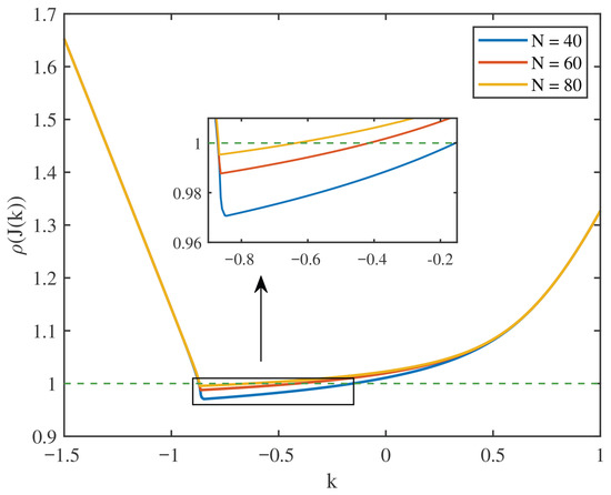
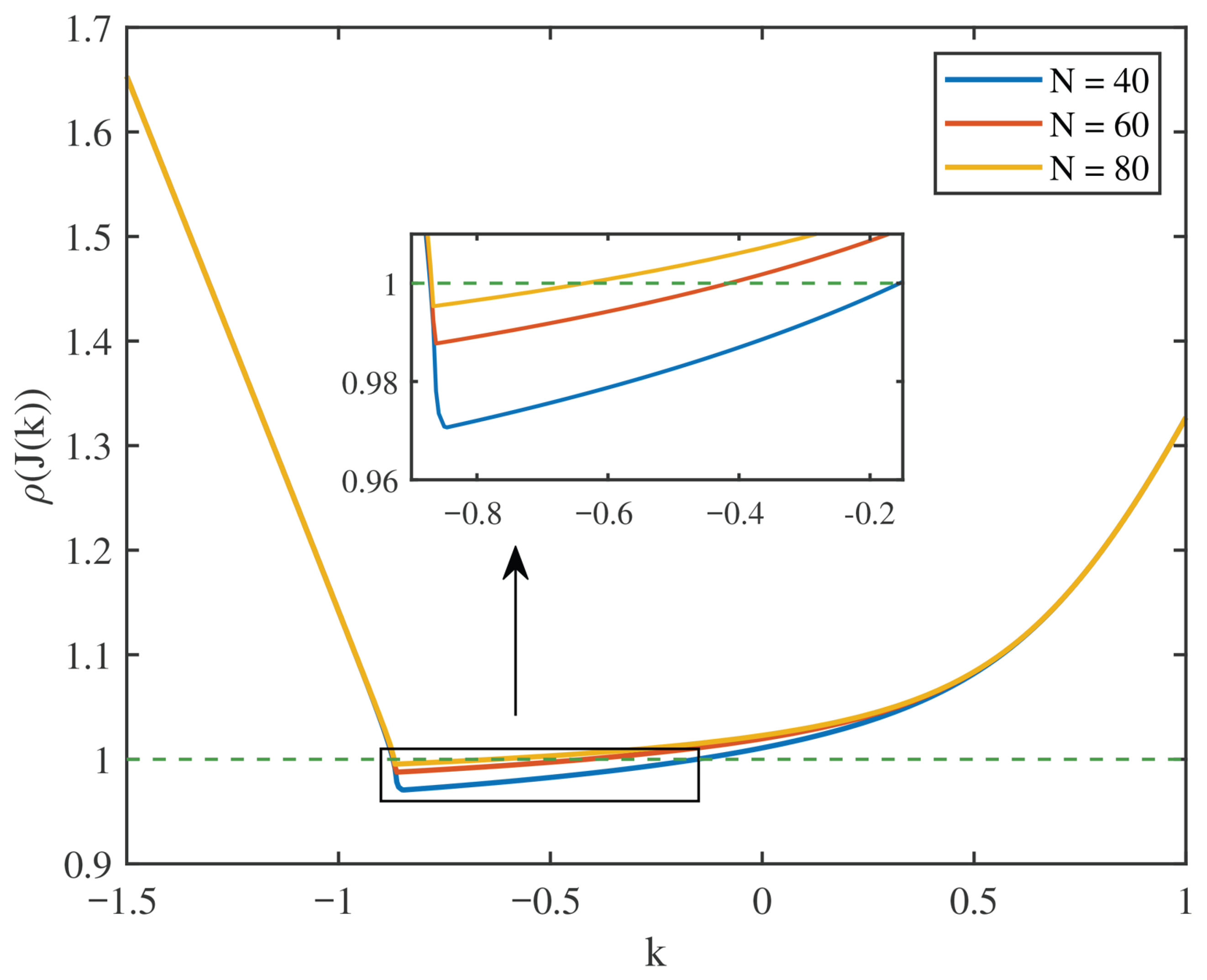
The change of the spectral radius $\rho \left(J\right(k\left)\right)$ of system (16) at the fixed point $F_e$ with respect to the control parameter k is calculated. To examine the influence of the memory length, we compare the spectral-radius curves for $N=40,60$ and 80, as shown in Figure 3. When $\rho \left(J\right)<1$, system (9) is stable. Numerically, the stable k-interval becomes wider for a smaller memory length (approximately $(-0.8708,-0.1583)$ for $N=40$), but it represents a shorter effective memory and thus weakens long-memory effects; in contrast, a larger memory length incorporates more past states yields a narrower admissible k-interval (approximately $(-0.8667,-0.6375)$ for $N=80$), resulting in a more restrictive control range. Therefore, we adopt the intermediate choice $N=60$, for which the numerical stable range is $k\in (-0.8667,-0.4167)$. From Theorem 1, it is known that system (16) is stable at the fixed point $F_e$, so the fixed point $(0.4000,0.0155,0.9832)$ of system (13) also remains locally stable within this k value range. Therefore, by adjusting the parameter k, the Julia set of system (13) is controlled.

Figure 3. Spectral radius $\rho \left(J\right(k\left)\right)$ at the fixed point $F_e$ versus k for system (16) with different N.

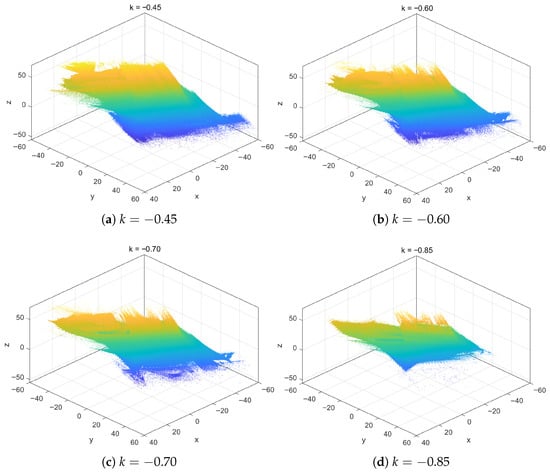
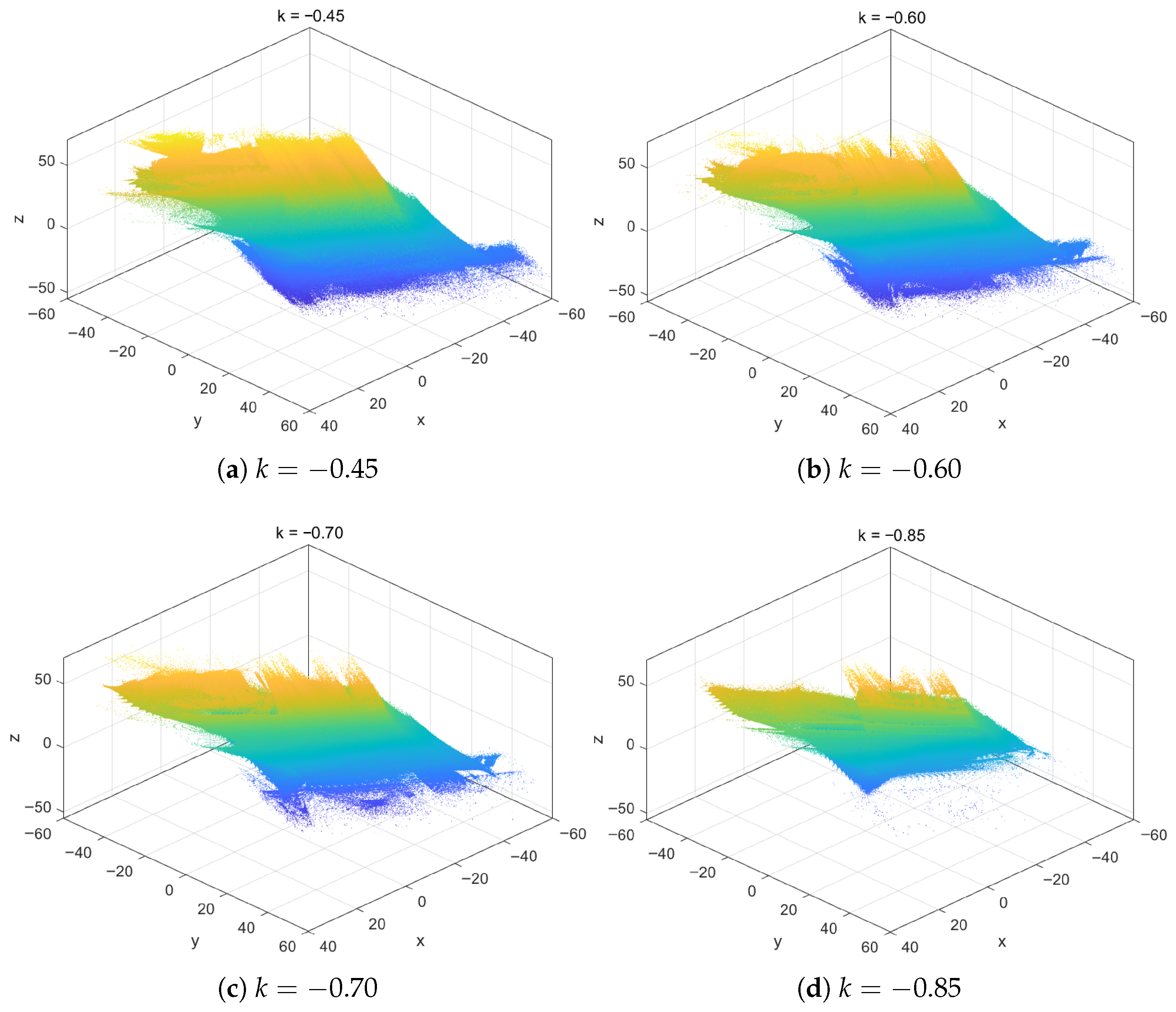
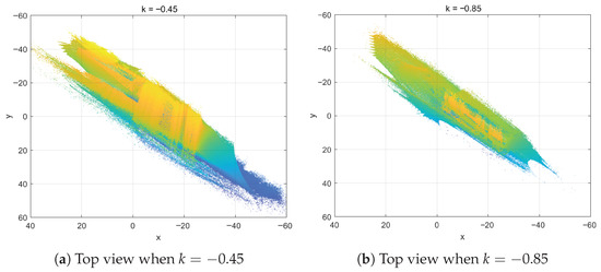
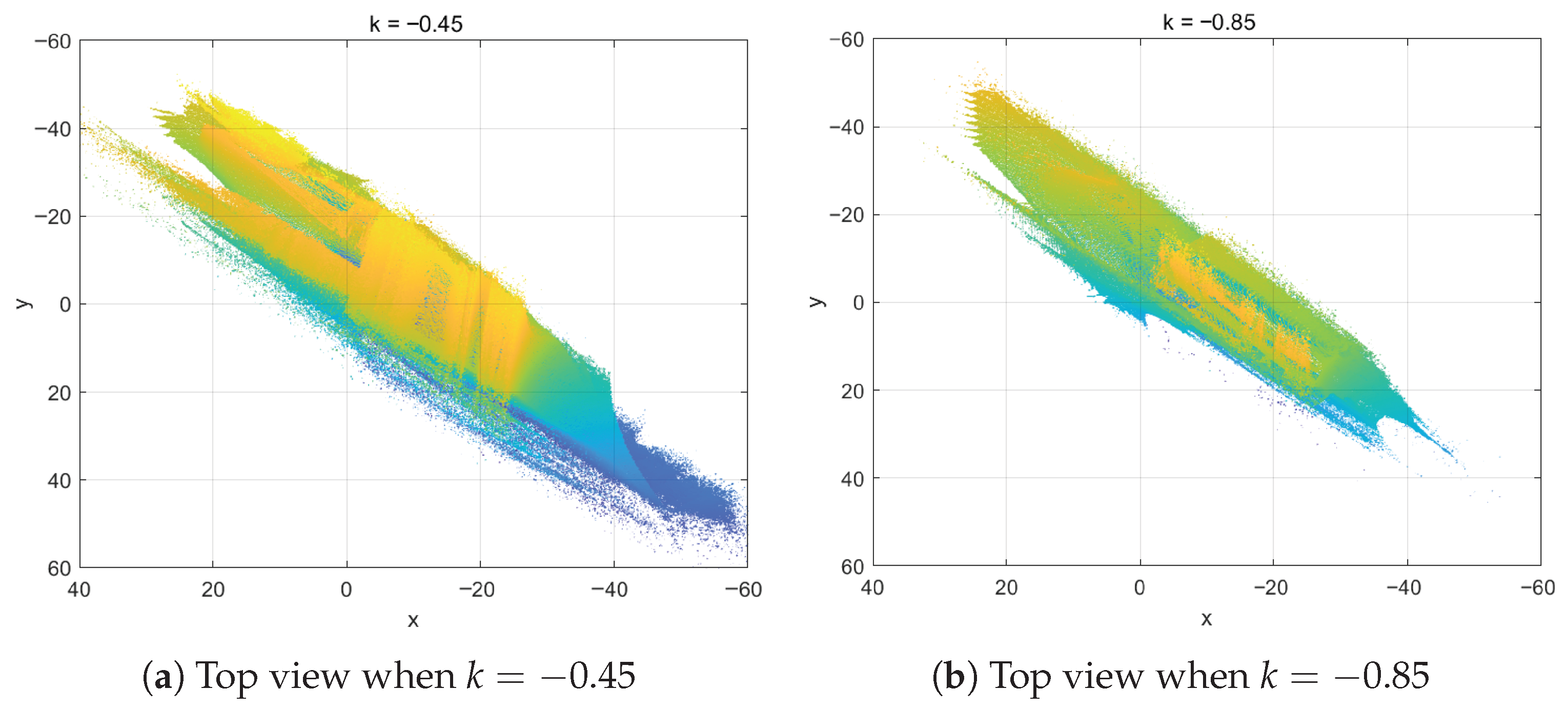
Figure 4 illustrates the filled Julia sets of system (13) for different values of the control parameter k within the stability region, and Figure 5 presents the top view of Figure 4a,d and provides a clearer visualization of the fractal structure. It can be found that as the control parameter k gradually decreases, the relatively irregular boundary structure of the filled Julia set gradually reduces its fractal details, and the overall coverage range of the filled Julia set shrinks accordingly, reflecting the effectiveness of the control method.

Figure 4. Control of filled Julia sets of system (13) under different parameters k.

Figure 5. Top view of Figure 4a,d.

Ecologically, control studies of infectious disease model aim to drive the system toward stable and sustainable evolutionary states, maintaining stability and reducing the risk of ecological imbalance due to outbreaks. Epidemiologically, the contraction of the filled Julia set implies that, within this range of the control parameter, the system’s bounded dynamical region becomes smaller, constraining the trajectories of disease-related variables to a narrower range, offering an intuitive characterization of the disease’s long-term controllability and manageability.

5. Synchronization of Julia Sets

The previous section studied the control problem of the Julia set of the HCV system (9). However, how to design control terms to make one Julia set tend to another Julia set is also worth studying. In this section, we study the synchronization of Julia sets between two discrete fractional-order systems with the same structure but different parameters and different fractional orders, by taking different values of $\beta$ and $\alpha$ in the HCV system (9).

Considering that only $\beta$ differs in the biological parameters of the two systems, and other parameters $B,c,\theta ,\mu$ remain consistent, for $X\in \{S,A,L\}$ and system number $i\in \{1,2\}$, let $E_{X,i}^{j-1}$ be

$$\left\{\begin{array}{cc}\hfill E_{S,i}^{j-1}& =B-{\beta }_i{S}_i(j-1)[A_i(j-1)+L_i(j-1)]+c{A}_i(j-1)-\mu S_i(j-1),\hfill \\ \hfill E_{A,i}^{j-1}& ={\beta }_i{S}_i(j-1)[A_i(j-1)+L_i(j-1)]-(c+\theta +\mu )A_i(j-1),\hfill \\ \hfill E_{L,i}^{j-1}& =\theta A_i(j-1)-\mu L_i(j-1).\hfill \end{array}\right.$$

Take the target system ($i=1$, parameters ${\alpha }_1,{\beta }_1$) as

$$\left\{\begin{array}{cc}\hfill S_1\left(n\right)& =S_1\left(0\right)+{\displaystyle \frac{1}{\Gamma \left({\alpha }_1\right)}}\sum _{j=1}^n{\displaystyle \frac{\Gamma (n-j+{\alpha }_1)}{\Gamma (n-j+1)}}{E}_{S,1}^{j-1},\hfill \\ \hfill A_1\left(n\right)& =A_1\left(0\right)+{\displaystyle \frac{1}{\Gamma \left({\alpha }_1\right)}}\sum _{j=1}^n{\displaystyle \frac{\Gamma (n-j+{\alpha }_1)}{\Gamma (n-j+1)}}{E}_{A,1}^{j-1},\hfill \\ \hfill L_1\left(n\right)& =L_1\left(0\right)+{\displaystyle \frac{1}{\Gamma \left({\alpha }_1\right)}}\sum _{j=1}^n{\displaystyle \frac{\Gamma (n-j+{\alpha }_1)}{\Gamma (n-j+1)}}{E}_{L,1}^{j-1}.\hfill \end{array}\right.$$

(17)

Take the response system ($i=2$, parameters ${\alpha }_2,{\beta }_2$) as

$$\left\{\begin{array}{cc}\hfill S_2\left(n\right)& =S_2\left(0\right)+{\displaystyle \frac{1}{\Gamma \left({\alpha }_2\right)}}\sum _{j=1}^n{\displaystyle \frac{\Gamma (n-j+{\alpha }_2)}{\Gamma (n-j+1)}}{E}_{S,2}^{j-1}+u_S\left(n\right),\hfill \\ \hfill A_2\left(n\right)& =A_2\left(0\right)+{\displaystyle \frac{1}{\Gamma \left({\alpha }_2\right)}}\sum _{j=1}^n{\displaystyle \frac{\Gamma (n-j+{\alpha }_2)}{\Gamma (n-j+1)}}{E}_{A,2}^{j-1}+u_A\left(n\right),\hfill \\ \hfill L_2\left(n\right)& =L_2\left(0\right)+{\displaystyle \frac{1}{\Gamma \left({\alpha }_2\right)}}\sum _{j=1}^n{\displaystyle \frac{\Gamma (n-j+{\alpha }_2)}{\Gamma (n-j+1)}}{E}_{L,2}^{j-1}+u_L\left(n\right).\hfill \end{array}\right.$$

(18)

where ${\alpha }_1\ne {\alpha }_2$ and ${\beta }_1\ne {\beta }_2$, and $u_X\left(n\right)$ ($X\in \{S,A,L\}$) is the coupling term. To achieve the synchronization of the Julia sets between system (17) and system (18), take the synchronization controller $u_X\left(n\right)$ as

$$\begin{array}{cc}\hfill u_X\left(n\right)& =l_1[\sum _{j=1}^{n-1}(\left({\displaystyle \genfrac{}{}{0pt}{}{n-j+{\alpha }_1-2}{n-1-j}}\right)E_{X,1}^{j-1}-\left({\displaystyle \genfrac{}{}{0pt}{}{n-j+{\alpha }_2-2}{n-1-j}}\right)E_{X,2}^{j-1})\hfill \\ & +(E_{X,1}^{n-1}-E_{X,2}^{n-1})]-l_2\sum _{j=1}^{n-1}[\left({\displaystyle \genfrac{}{}{0pt}{}{n-j+{\alpha }_2-2}{n-j}}\right)E_{X,2}^{j-1}-\left({\displaystyle \genfrac{}{}{0pt}{}{n-j+{\alpha }_1-2}{n-j}}\right)E_{X,1}^{j-1}].\hfill \end{array}$$

(19)

where $l_1,l_2$ are control parameters.

Theorem 2.

When $l_1\to 1,l_2\to 1$, $|X_2\left(n\right)-X_1\left(n\right)|\to 0$ holds, that is, the synchronization between system (17) and system (18) is achieved, thereby achieving the synchronization of the Julia sets.

Proof. 

Let $F_X\left(n\right)=X_2\left(n\right)-X_1\left(n\right)$, and $X_1\left(0\right)=X_2\left(0\right)$. Substituting Equation (19) into system (18), since ${\displaystyle \frac{1}{\Gamma \left(\alpha \right)}}{\displaystyle \frac{\Gamma (n-j+\alpha )}{\Gamma (n-j+1)}}=\left({\displaystyle \genfrac{}{}{0pt}{}{n-j+\alpha -1}{n-j}}\right)$, then

$$\begin{array}{ccc}\hfill F_X\left(n\right)& =\sum _{j=1}^{n-1}[\left({\displaystyle \genfrac{}{}{0pt}{}{n-j+{\alpha }_2-1}{n-j}}\right)E_{X,2}^{j-1}-\left({\displaystyle \genfrac{}{}{0pt}{}{n-j+{\alpha }_1-1}{n-j}}\right)E_{X,1}^{j-1}]\hfill & \\ & +l_1\sum _{j=1}^{n-1}[\left({\displaystyle \genfrac{}{}{0pt}{}{n-j+{\alpha }_1-2}{n-1-j}}\right)E_{X,1}^{j-1}-\left({\displaystyle \genfrac{}{}{0pt}{}{n-j+{\alpha }_2-2}{n-1-j}}\right)E_{X,2}^{j-1}]\hfill & \\ & +(1-l_1)(E_{X,2}^{n-1}-E_{X,1}^{n-1})-l_2\sum _{j=1}^{n-1}[\left({\displaystyle \genfrac{}{}{0pt}{}{n-j+{\alpha }_2-2}{n-j}}\right)E_{X,2}^{j-1}\hfill & \\ & -\left({\displaystyle \genfrac{}{}{0pt}{}{n-j+{\alpha }_1-2}{n-j}}\right)E_{X,1}^{j-1}]\hfill & \\ & =l_1\sum _{j=1}^{n-1}[(\left({\displaystyle \genfrac{}{}{0pt}{}{n-j+{\alpha }_2-1}{n-j}}\right)-\left({\displaystyle \genfrac{}{}{0pt}{}{n-j+{\alpha }_2-2}{n-1-j}}\right))E_{X,2}^{j-1}-(\left({\displaystyle \genfrac{}{}{0pt}{}{n-j+{\alpha }_1-1}{n-j}}\right)\hfill & \\ & -\left({\displaystyle \genfrac{}{}{0pt}{}{n-j+{\alpha }_1-2}{n-1-j}}\right))E_{X,1}^{j-1}]+(1-l_1)\sum _{j=1}^{n-1}[\left({\displaystyle \genfrac{}{}{0pt}{}{n-j+{\alpha }_2-1}{n-j}}\right)E_{X,2}^{j-1}\hfill & \\ & -\left({\displaystyle \genfrac{}{}{0pt}{}{n-j+{\alpha }_1-1}{n-j}}\right)E_{X,1}^{j-1}]+(1-l_1)(E_{X,2}^{n-1}-E_{X,1}^{n-1})\hfill & \\ & -l_2\sum _{j=1}^{n-1}[\left({\displaystyle \genfrac{}{}{0pt}{}{n-j+{\alpha }_2-2}{n-j}}\right)E_{X,2}^{j-1}-\left({\displaystyle \genfrac{}{}{0pt}{}{n-j+{\alpha }_1-2}{n-j}}\right)E_{X,1}^{j-1}].\hfill \end{array}$$

For any $0<\alpha <1$, $\left({\displaystyle \genfrac{}{}{0pt}{}{n-j+\alpha -1}{n-j}}\right)-\left({\displaystyle \genfrac{}{}{0pt}{}{n-j+\alpha -2}{n-1-j}}\right)=\left({\displaystyle \genfrac{}{}{0pt}{}{n-j+\alpha -2}{n-j}}\right)$; thus, we can obtain

$$\begin{array}{ccc}\hfill F_X\left(n\right)& =l_1\sum _{j=1}^{n-1}[\left({\displaystyle \genfrac{}{}{0pt}{}{n-j+{\alpha }_2-2}{n-j}}\right)E_{X,2}^{j-1}-\left({\displaystyle \genfrac{}{}{0pt}{}{n-j+{\alpha }_1-2}{n-j}}\right)E_{X,1}^{j-1}]\hfill & \\ & +(1-l_1)\sum _{j=1}^{n-1}[\left({\displaystyle \genfrac{}{}{0pt}{}{n-j+{\alpha }_2-1}{n-j}}\right)E_{X,2}^{j-1}-\left({\displaystyle \genfrac{}{}{0pt}{}{n-j+{\alpha }_1-1}{n-j}}\right)E_{X,1}^{j-1}]\hfill & \\ & +(1-l_1)(E_{X,2}^{n-1}-E_{X,1}^{n-1})-l_2\sum _{j=1}^{n-1}[\left({\displaystyle \genfrac{}{}{0pt}{}{n-j+{\alpha }_2-2}{n-j}}\right)E_{X,2}^{j-1}\hfill & \\ & -\left({\displaystyle \genfrac{}{}{0pt}{}{n-j+{\alpha }_1-2}{n-j}}\right)E_{X,1}^{j-1}].\hfill \end{array}$$

Here, to simplify notation, let $F_{X,i}^{j-1}=E_{X,i}^{j-1}+X_i(j-1)$, then $E_{X,2}^{n-1}-E_{X,1}^{n-1}=F_{X,2}^{n-1}-X_2(n-1)-(F_{X,1}^{n-1}-X_1(n-1))=F_{X,2}^{n-1}-F_{X,1}^{n-1}-F_X(n-1)$,

$$\begin{array}{ccc}\hfill F_X\left(n\right)& =(l_1-l_2)\sum _{j=1}^{n-1}[\left({\displaystyle \genfrac{}{}{0pt}{}{n-j+{\alpha }_2-2}{n-j}}\right)E_{X,2}^{j-1}-\left({\displaystyle \genfrac{}{}{0pt}{}{n-j+{\alpha }_1-2}{n-j}}\right)E_{X,1}^{j-1}]\hfill & \\ & +(1-l_1)\sum _{j=1}^{n-1}[\left({\displaystyle \genfrac{}{}{0pt}{}{n-j+{\alpha }_2-1}{n-j}}\right)E_{X,2}^{j-1}-\left({\displaystyle \genfrac{}{}{0pt}{}{n-j+{\alpha }_1-1}{n-j}}\right)E_{X,1}^{j-1}]\hfill & \\ & +(1-l_1)\left(F_{X,2}^{n-1}-F_{X,1}^{n-1}\right)+(l_1-1)F_X(n-1).\hfill \end{array}$$

From the expression of $F_X\left(n\right)$, $F_X(n-1)$ can be obtained; thus,

$$\begin{array}{ccc}\hfill F_X\left(n\right)-F_X(n-1)& =(l_1-l_2)\sum _{j=1}^{n-1}[\left({\displaystyle \genfrac{}{}{0pt}{}{n-j+{\alpha }_2-2}{n-j}}\right)E_{X,2}^{j-1}-\left({\displaystyle \genfrac{}{}{0pt}{}{n-j+{\alpha }_1-2}{n-j}}\right)E_{X,1}^{j-1}]\hfill & \\ & -(l_1-l_2)\sum _{j=1}^{n-2}[\left({\displaystyle \genfrac{}{}{0pt}{}{n-j+{\alpha }_2-3}{n-1-j}}\right)E_{X,2}^{j-1}-\left({\displaystyle \genfrac{}{}{0pt}{}{n-j+{\alpha }_1-3}{n-1-j}}\right)E_{X,1}^{j-1}]\hfill & \\ & +(1-l_1)\sum _{j=1}^{n-1}[(\left({\displaystyle \genfrac{}{}{0pt}{}{n-j+{\alpha }_2-1}{n-j}}\right)-\left({\displaystyle \genfrac{}{}{0pt}{}{n-j+{\alpha }_2-2}{n-1-j}}\right))E_{X,2}^{j-1}\hfill & \\ & -[\left({\displaystyle \genfrac{}{}{0pt}{}{n-j+{\alpha }_1-1}{n-j}}\right)-\left({\displaystyle \genfrac{}{}{0pt}{}{n-j+{\alpha }_1-2}{n-1-j}}\right)]E_{X,1}^{j-1}]\hfill & \\ & +(1-l_1)(F_{X,2}^{n-1}-F_{X,1}^{n-1})+(l_1-1)F_X(n-1).\hfill \end{array}$$

Similarly, noting that $\left({\displaystyle \genfrac{}{}{0pt}{}{n-j+\alpha -1}{n-j}}\right)-\left({\displaystyle \genfrac{}{}{0pt}{}{n-j+\alpha -2}{n-1-j}}\right)=\left({\displaystyle \genfrac{}{}{0pt}{}{n-j+\alpha -2}{n-j}}\right)$, then we can obtain

$$\begin{array}{ccc}\hfill F_X\left(n\right)-F_X(n-1)& =(1-l_2)\sum _{j=1}^{n-1}[\left({\displaystyle \genfrac{}{}{0pt}{}{n-j+{\alpha }_2-2}{n-j}}\right)E_{X,2}^{j-1}-\left({\displaystyle \genfrac{}{}{0pt}{}{n-j+{\alpha }_1-2}{n-j}}\right)E_{X,1}^{j-1}]\hfill & \\ & -(l_1-l_2)\sum _{j=1}^{n-2}[\left({\displaystyle \genfrac{}{}{0pt}{}{n-j+{\alpha }_2-3}{n-1-j}}\right)E_{X,2}^{j-1}-\left({\displaystyle \genfrac{}{}{0pt}{}{n-j+{\alpha }_1-3}{n-1-j}}\right)E_{X,1}^{j-1}]\hfill & \\ & +(1-l_1)(F_{X,2}^{n-1}-F_{X,1}^{n-1})+(l_1-1)F_X(n-1).\hfill \end{array}$$

Since for any $0<\alpha <1$, we have $\left({\displaystyle \genfrac{}{}{0pt}{}{n-j+\alpha -2}{n-j}}\right)={\displaystyle \frac{(n-j+\alpha -2)(n-j+\alpha -3)\cdots (\alpha -1)}{(n-j)!}}<0$, $\left({\displaystyle \genfrac{}{}{0pt}{}{n-j+\alpha -3}{n-1-j}}\right)={\displaystyle \frac{(n-j+\alpha -3)(n-j+\alpha -4)\cdots (\alpha -1)}{(n-1-j)!}}<0$, and we can obtain

$$\begin{array}{ccc}\hfill \left|F_X\left(n\right)\right|& \le |l_1||F_X(n-1)|-|1-l_2|\sum _{j=1}^{n-1}[\left({\displaystyle \genfrac{}{}{0pt}{}{n-j+{\alpha }_2-2}{n-j}}\right)|E_{X,2}^{j-1}|\hfill & \\ & +\left({\displaystyle \genfrac{}{}{0pt}{}{n-j+{\alpha }_1-2}{n-j}}\right)|E_{X,1}^{j-1}|]-|l_1-l_2|\sum _{j=1}^{n-2}[\left({\displaystyle \genfrac{}{}{0pt}{}{n-j+{\alpha }_2-3}{n-1-j}}\right)|E_{X,2}^{j-1}|\hfill & \\ & +\left({\displaystyle \genfrac{}{}{0pt}{}{n-j+{\alpha }_1-3}{n-1-j}}\right)|E_{X,1}^{j-1}|]+|1-l_1||F_{X,2}^{n-1}-F_{X,1}^{n-1}|.\hfill \end{array}$$

From the Definition 1, points inside the filled Julia set of (17) and (18) remain bounded throughout the iteration process. Hence, there exists a constant $R>0$, such that $|S_i\left(j\right)|,|A_i\left(j\right)|,|L_i\left(j\right)|\le R$, $i\in \{1,2\}$. Consequently, each $E_{X,i}^{j-1}$ is bounded and there exists constants $M_{X,i}>0$, such that $|E_{X,i}^{j-1}|\le M_{X,i}$. Moreover, since $F_{X,i}^{j-1}=E_{X,i}^{j-1}+X_i(j-1)$, there exists constants $N_{X,i}>0$ such that $|F_{X,i}^{j-1}|\le N_{X,i}$. Therefore, we have

$$\begin{array}{ccc}\hfill |F_X\left(n\right)|& \le \left|l_1\right||F_X(n-1)|-|1-l_2|\sum _{j=1}^{n-1}[\left({\displaystyle \genfrac{}{}{0pt}{}{n-j+{\alpha }_2-2}{n-j}}\right)M_{X,2}\hfill & \\ & +\left({\displaystyle \genfrac{}{}{0pt}{}{n-j+{\alpha }_1-2}{n-j}}\right)M_{X,1}]-|l_1-l_2|\sum _{j=1}^{n-2}[\left({\displaystyle \genfrac{}{}{0pt}{}{n-j+{\alpha }_2-3}{n-1-j}}\right)M_{X,2}\hfill & \\ & +\left({\displaystyle \genfrac{}{}{0pt}{}{n-j+{\alpha }_1-3}{n-1-j}}\right)M_{X,1}]+|1-l_1|(N_{X,2}+N_{X,1}).\hfill \end{array}$$

Since for any $0<\alpha <1$, we have

$$\begin{array}{c}\sum _{j=1}^{n-1}\left({\displaystyle \genfrac{}{}{0pt}{}{n-j+\alpha -2}{n-j}}\right)=\left({\displaystyle \genfrac{}{}{0pt}{}{n-2+\alpha }{n-1}}\right)-1,\sum _{j=1}^{n-2}\left({\displaystyle \genfrac{}{}{0pt}{}{n-j+\alpha -3}{n-1-j}}\right)=\left({\displaystyle \genfrac{}{}{0pt}{}{n-3+\alpha }{n-2}}\right)-1,\\ \left({\displaystyle \genfrac{}{}{0pt}{}{n-2+\alpha }{n-1}}\right)={\displaystyle \frac{(n-2+\alpha )(n-3+\alpha )\dots \alpha }{(n-1)!}}>0,\\ \left({\displaystyle \genfrac{}{}{0pt}{}{n-3+\alpha }{n-2}}\right)={\displaystyle \frac{(n-3+\alpha )(n-4+\alpha )\dots \alpha }{(n-2)!}}>0.\end{array}$$

Therefore, we can obtain

$$\begin{array}{c}0<-\sum _{j=1}^{n-1}\left({\displaystyle \genfrac{}{}{0pt}{}{n-j+\alpha -2}{n-j}}\right)<1,0<-\sum _{j=1}^{n-2}\left({\displaystyle \genfrac{}{}{0pt}{}{n-j+\alpha -3}{n-1-j}}\right)<1.\end{array}$$

Thus

$$\begin{array}{c}\left|F_X\left(n\right)\right|\le \left|l_1\right|\left|F_X(n-1)\right|+(|1-l_2|+|l_1-l_2|)(M_{X,2}+M_{X,1})+|1-l_1|(N_{X,2}+N_{X,1}).\end{array}$$

When $l_1\to 1,l_2\to 1$, we have $|1-l_2|\to 0,|l_1-l_2|\to 0,|1-l_1|\to 0$, from this we can obtain $\left|F_X\left(n\right)\right|\le |F_X(n-1)|\le \cdots \le |F_X\left(0\right)|$. Given $F_X\left(0\right)=0$, then it can be deduced that $|F_X\left(n\right)|\to 0$, and further from Definition 1, it is known that the synchronization of the Julia sets between system (17) and system (18) is achieved. □

Next, the effectiveness of this synchronization scheme is illustrated through numerical simulation. Set the common parameters of the target system (17) and the response system (18) as $B=0.0221, \mu =0.0158, \theta =1, c=0.27$, the parameters of the target system (17) as ${\beta }_1=0.05, {\alpha }_1=0.7$, and the parameters of the response system (18) as ${\beta }_2=0.07, {\alpha }_2=0.5$.

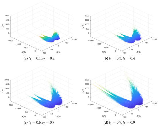
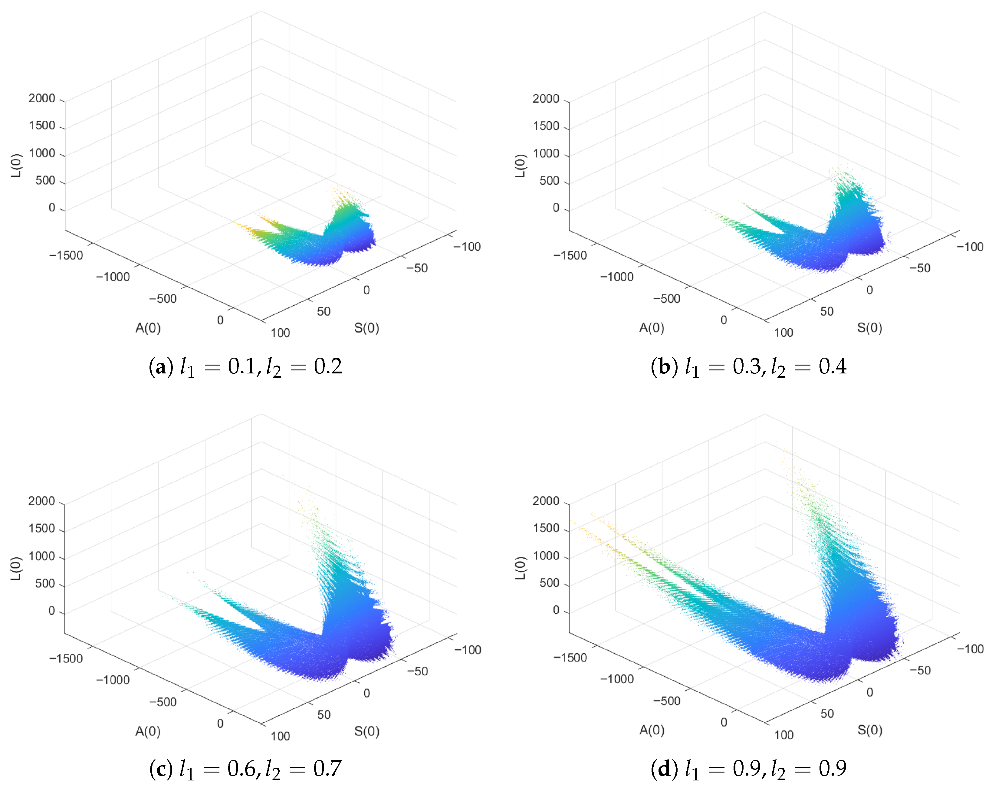
As shown in Figure 6, it can be found that as the values of the control coefficients $l_1$ and $l_2$ gradually approach 1, the two wings of the butterfly shape of the Julia set of the response system (18) continue to expand, gradually approaching the morphology of the Julia set of the target system (17), which are referred to in Figure 1c.

Figure 6. The synchronization between the Julia sets of system (17) and system (18) when parameters $l_1,l_2$ change.

Comparing Figure 2a with Figure 7b, it can be seen that when the control coefficients $l_1,l_2$ are close to 1, the Julia set of the response system (18) is basically consistent with the Julia set of the target system (17) in terms of the details and morphology of the butterfly’s two wings, intuitively achieving the synchronization of the Julia sets between the two systems.

Figure 7. Top view of Figure 6a,d.

From a biological and ecological perspective, the synchronization of epidemic systems reflects the coordinated evolution of disease dynamics among different populations or spatial regions under coupling effects such as migration and environmental interactions. In fractional-order epidemic models, synchronization further indicates that heterogeneous populations with different memory effects and transmission characteristics may still exhibit coherent epidemic behaviors. Such results provide insights into the propagation mechanisms of infectious diseases in ecological systems and offer theoretical support for epidemic control strategies.

6. Conclusions

This paper investigates the fractal dynamical behavior of the three-dimensional fractional-order HCV model and explores the control and synchronization of its Julia sets. The stability of the system is examined by evaluating the spectral radius of the Jacobian matrix at the fixed point. Based on the coordinate transformation, suitable control terms are then designed to regulate the system. In addition, a nonlinear coupling controller is developed to realize synchronization between two HCV systems with different parameters and different fractional orders. Rigorous theoretical analyses and numerical simulations are provided to validate the proposed results. The proposed control and synchronization methods are applicable to models in other fields. Moreover, the fractal–fractional operator can be considered as an alternative to the Caputo operator, enabling a tighter integration of fractional-order calculus with fractal dynamics.

References

- Kraef, C.; Bentzon, A.; Skrahina, A.; Mocroft, A.; Peters, L.; Lundgren, J.D.; Chkhartishvili, N.; Podlekareva, D.; Kirk, O. Improving healthcare for patients with HIV, tuberculosis and hepatitis C in Eastern Europe: A review of current challenges and important next steps. HIV Med. 2022, 23, 48–59. [Google Scholar] [CrossRef] [Scilit]
- Wiktor, S.; Ford, N.; Ball, A.; Hirnschall, G. HIV and HCV: Distinct infections with important overlapping challenges. J. Int. Aids Soc. 2014, 17, 19323. [Google Scholar] [CrossRef] [Scilit] [PubMed]
- Woyesa, S.B.; Amente, K.D. Hepatitis C virus dynamic transmission models among people who inject drugs. Infect. Drug Resist. 2023, 16, 1061–1068. [Google Scholar] [CrossRef] [Scilit]
- Martcheva, M.; Castillo-Chavez, C. Diseases with chronic stage in a population with varying size. Math. Biosci. 2003, 182, 1–25. [Google Scholar] [CrossRef] [Scilit]
- Vickerman, P.; Hickman, M.; Judd, A. Modelling the impact on Hepatitis C transmission of reducing syringe sharing: London case study. Int. J. Epidemiol. 2007, 36, 396–405. [Google Scholar] [CrossRef] [Scilit]
- Vickerman, P.; Miners, A.; Williams, J. Assessing the Cost-Effectiveness of Interventions Linked to Needle and Syringe Programmes for Injecting Drug Users; NICE: London, UK, 2008. [Google Scholar]
- Helikumi, M.; Mushanyu, J.; Mhlanga, A. A mathematical model of HCV transmission dynamics with sex stratification and environmental effects. PLoS ONE 2025, 20, e0336374. [Google Scholar] [CrossRef] [Scilit] [PubMed]
- Das, P.; Mukherjee, D.; Sarkar, A. Analysis of a disease transmission model of hepatitis C. J. Biol. Syst. 2005, 13, 331–339. [Google Scholar] [CrossRef] [Scilit]
- Shen, M.; Xiao, Y.; Zhou, W.; Li, Z. Global dynamics and applications of an epidemiological model for hepatitis C virus transmission in China. Discret. Dyn. Nat. Soc. 2015, 2015, 543029. [Google Scholar] [CrossRef] [Scilit]
- Carvalho, A.R.; Pinto, C.M. A coinfection model for HIV and HCV. Biosystems 2014, 124, 46–60. [Google Scholar] [CrossRef] [Scilit]
- Korkmaz, I.; Araz, S.I. New perspectives on Hepatitis C model with Piecewise Derivative: Deterministic and Stochastic Approaches. J. Prime Res. Math. 2025, 21, 101–118. [Google Scholar]
- Naik, P.A.; Yeolekar, B.M.; Qureshi, S.; Yeolekar, M.; Madzvamuse, A. Modeling and analysis of the fractional-order epidemic model to investigate mutual influence in HIV/HCV co-infection. Nonlinear Dyn. 2024, 112, 11679–11710. [Google Scholar] [CrossRef] [Scilit]
- Saleem, A.; ur Rahman, M.; Boulaaras, S.; Guefaifia, R.; Baleanu, D. Exploring the dynamics of HIV and HCV co-infection through piecewise modified Mittag-Leffler fractional derivatives. Appl. Math. Sci. Eng. 2025, 33, 2478038. [Google Scholar] [CrossRef] [Scilit]
- Saad, K.M.; Alqhtani, M.; Gómez-Aguilar, J. Fractal-fractional study of the hepatitis C virus infection model. Results Phys. 2020, 19, 103555. [Google Scholar] [CrossRef] [Scilit]
- Ali, M.A.; Liu, W.; Furuichi, S.; Fečkan, M. Improved Hermite–Hadamard inequality bounds for Riemann–Liouville fractional integrals via jensen’s inequality. Fractal Fract. 2024, 8, 547. [Google Scholar] [CrossRef] [Scilit]
- Elgezouli, D.E.; Eltayeb, H.; Abdoon, M.A. Novel GPID: Grünwald–Letnikov fractional PID for enhanced adaptive cruise control. Fractal Fract. 2024, 8, 751. [Google Scholar] [CrossRef] [Scilit]
- Karaoğlan, A.; Set, E.; Akdemir, A.O.; Özdemir, M.E. Fractional integral inequalities for preinvex functions via Atangana-Baleanu integral operators. Miskolc Math. Notes 2024, 25, 329–347. [Google Scholar] [CrossRef] [Scilit]
- Sun, W.; He, X. Hermite-Hadamard type inequalities and convex functions in signal processing. IEEE Access 2024, 12, 92906–92918. [Google Scholar] [CrossRef] [Scilit]
- Atici, F.M.; Eloe, P.W. Initial value problems in discrete fractional calculus. Proc. Am. Math. Soc. 2009, 137, 981–989. [Google Scholar] [CrossRef] [Scilit]
- Abdeljawad, T. On Riemann and Caputo fractional differences. Comput. Math. Appl. 2011, 62, 1602–1611. [Google Scholar] [CrossRef] [Scilit]
- Khan, A.Q.; Ayesha, Y.; Alsaadi, A. Discrete Hepatitis C virus model with local dynamics, chaos and bifurcations. AIMS Math. 2024, 9, 28643–28670. [Google Scholar] [CrossRef] [Scilit]
- Coll, C.; Herrero, A.; Ginestar, D.; Sánchez, E. The discrete fractional order difference applied to an epidemic model with indirect transmission. Appl. Math. Model. 2022, 103, 636–648. [Google Scholar] [CrossRef] [Scilit]
- Wang, Y.; Liu, S.; Li, H.; Wang, D. On the spatial Julia set generated by fractional Lotka-Volterra system with noise. Chaos Solitons Fractals 2019, 128, 129–138. [Google Scholar] [CrossRef] [Scilit]
- Ouyang, M.; Zhang, Y. Julia sets and their control of discrete fractional SIRS models. Complexity 2019, 2019, 5059025. [Google Scholar] [CrossRef] [Scilit]
- Wang, Y.; Liu, S.; Li, H. On fractional difference logistic maps: Dynamic analysis and synchronous control. Nonlinear Dyn. 2020, 102, 579–588. [Google Scholar] [CrossRef] [Scilit]
- Lu, X.; Sun, W. Control and synchronization of Julia sets of discrete fractional Ising models. Chaos Solitons Fractals 2024, 180, 114541. [Google Scholar] [CrossRef] [Scilit]
- Kumar, M.; Abbas, S. Fractal dimension and control of Julia set generated by the discrete competitive model. Numer. Algorithms 2026, 101, 643–678. [Google Scholar] [CrossRef] [Scilit]
- Wang, Y.; Liu, S. Fractal analysis and control of the fractional Lotka–Volterra model. Nonlinear Dyn. 2019, 95, 1457–1470. [Google Scholar] [CrossRef] [Scilit]
- Wang, Y.; Liu, S.; Li, H. Adaptive synchronization of Julia sets generated by Mittag–Leffler function. Commun. Nonlinear Sci. Numer. Simul. 2020, 83, 105115. [Google Scholar] [CrossRef] [Scilit]
- Danca, M.F.; Fečkan, M. Mandelbrot set and Julia sets of fractional order. Nonlinear Dyn. 2023, 111, 9555–9570. [Google Scholar] [CrossRef] [Scilit]
- Elsadany, A.; Aldurayhim, A.; Agiza, H.; Elsonbaty, A. On the fractional-order complex cosine map: Fractal analysis, Julia set control and synchronization. Mathematics 2023, 11, 727. [Google Scholar] [CrossRef] [Scilit]
- Peitgen, H.O.; Richter, P.H. The Beauty of Fractals: Images of Complex Dynamical Systems; Springer Science & Business Media: Berlin/Heidelberg, Germany, 1986. [Google Scholar]
- Chen, F.; Luo, X.; Zhou, Y. Existence results for nonlinear fractional difference equation. Adv. Differ. Equ. 2011, 2011, 713201. [Google Scholar] [CrossRef] [Scilit]
- Zhao, Z.; Yang, M.; Lv, J.; Hu, Q.; Chen, Q.; Lei, Z.; Wang, M.; Zhang, H.; Zhai, X.; Zhao, B.; et al. Shigellosis seasonality and transmission characteristics in different areas of China: A modelling study. Infect. Dis. Model. 2022, 7, 161–178. [Google Scholar] [CrossRef] [Scilit]
- Wu, G.C.; Baleanu, D. Chaos synchronization of the discrete fractional logistic map. Signal Process. 2014, 102, 96–99. [Google Scholar] [CrossRef] [Scilit]
- Fandio, R.; Abboubakar, H.; Banbeto, S.A.G.; Ekobena, H.P. Mathematical modeling of the Cholera epidemic in Cameroon: From classical-order derivative to fractional-order derivative. MJ Math. Comput. Sci. 2025, 1, 1–32. [Google Scholar] [CrossRef] [Scilit]
- Ouyang, M.; Zhang, Y.; Liu, J. Fractal control and synchronization of the discrete fractional SIRS model. Complexity 2020, 2020, 3085036. [Google Scholar] [CrossRef] [Scilit]
- Grobman, D.M. Homeomorphism of systems of differential equations. Dokl. Akad. Nauk. SSSR 1959, 128, 880–881. [Google Scholar]
- Hartman, P. A lemma in the theory of structural stability of differential equations. Proc. Am. Math. Soc. 1960, 11, 610–620. [Google Scholar] [CrossRef]
Disclaimer/Publisher’s Note: The statements, opinions and data contained in all publications are solely those of the individual author(s) and contributor(s) and not of MDPI and/or the editor(s). MDPI and/or the editor(s) disclaim responsibility for any injury to people or property resulting from any ideas, methods, instructions or products referred to in the content. |
© 2026 by the authors. Licensee MDPI, Basel, Switzerland. This article is an open access article distributed under the terms and conditions of the Creative Commons Attribution (CC BY) license.