Article

An Efficient Solver for Fractional Diffusion on Unbounded Combs with Exact Absorbing Boundary Conditions

1
Center for Applied Mathematics of Guangxi, School of Mathematical Sciences, Guangxi Minzu University, Nanning 530006, China
2
Guangxi Higher Education Institutions Engineering Research Center of Low-Altitude Flight Guidance and Control, Nanning 530006, China
3
School of Science, Southwest Petroleum University, Chengdu 610500, China
*
Author to whom correspondence should be addressed.
Fractal Fract. 2026, 10(3), 208; https://doi.org/10.3390/fractalfract10030208
Submission received: 20 January 2026 / Revised: 2 March 2026 / Accepted: 10 March 2026 / Published: 23 March 2026
(This article belongs to the Section Numerical and Computational Methods)

Abstract

Despite its importance in modeling subdiffusion in fractal and heterogeneous media, a rigorous and computational scheme for solving the fractional diffusion equation on generalized comb structures over unbounded domains has remained elusive, mainly due to the nonlocal memory effect and slow spatial decay of solutions. To the best of our knowledge, we address this long-standing gap by presenting a fully integrated framework that simultaneously resolves both challenges. We derive the governing equation from constitutive relations and establish exact absorbing boundary conditions (ABCs) for the multi-skeleton comb model, a result absent in prior work. A transparent Dirichlet-to-Neumann (DtN) map, constructed via Laplace analysis, rigorously handles skeletal Dirac delta singularities and eliminates spurious reflections without empirical parameters. Furthermore, we propose a novel structure-preserving finite difference scheme that applies the sum-of-exponentials (SOE) approximation not only to the interior Caputo derivative but also to the convolution kernels arising from the ABCs. This yields a dramatic reduction in computational complexity, from quadratic O ( N t 2 ) to quasi-linear O ( N t log N t ) , while preserving the physics of anomalous transport. We prove the well-posedness, unconditional stability, and convergence of the method. Numerical results confirm theoretical error estimates and show excellent agreement between simulated particle distributions, mean square displacement profiles, and exact asymptotics, validating both accuracy and robustness. The speedup (CPU time ratio Direct/Fast) is about 1.00 × 1.23 × for N t = 5000 in our tests. Our approach sets a new benchmark for simulating anomalous dynamics in fractal-inspired media.

1. Introduction

Anomalous diffusion, distinguished by the non-linear power-law scaling of the mean squared displacement (MSD), x 2 ( t ) t α , has fundamentally transformed the theoretical landscape of transport phenomena in complex, heterogeneous media [1]. This departure from classical Brownian motion [2,3] ( α = 1 ) transcends theoretical abstraction, emerging as a ubiquitous mechanism across a wide spectrum of scientific disciplines. Recent investigations have elucidated its critical role in diverse physical scenarios, ranging from fluid transport in fractured porous reservoirs and charge carrier dynamics in disordered organic semiconductors to intracellular macromolecular crowding, where viscoelasticity governs particle trajectories. To provide a rigorous quantitative description of these non-local and memory-dependent processes, fractional calculus has served as the preeminent mathematical framework [4]. In particular, kinetic models employing the Caputo time-fractional derivative have proven exceptionally effective in characterizing subdiffusive regimes ( α < 1 ) induced by geometric confinement and energetic trapping mechanisms. To anchor this fractional kinetic formalism to specific geometric constraints, we identify the comb model as the canonical archetype that intrinsically generates confinement-induced retardation while reflecting the fractal nature of disordered media [5,6,7]. This structure, representing the backbone of percolation clusters near criticality [8], provides a minimal yet physically faithful proxy for anomalous transport.
To mathematically characterize transport within these intricate geometries, we adopt the generalized grid framework established by Sandev et al. [9,10]. We consider a configuration comprising N parallel backbones situated at transverse coordinates y = l j ( j = 1 , , N , ordered such that 0 l 1 < < l N ). Each backbone is associated with a non-negative structural weight w j , satisfying the normalization condition j = 1 N w j = 1 . Under the assumption of classical Fickian diffusion, the dynamics on this multi-backbone structure are governed by [9]
P ( x , y , t ) t = D x j = 1 N w j δ ( y l j ) 2 P ( x , y , t ) x 2 + D y 2 P ( x , y , t ) y 2 ,
where P ( x , y , t ) denotes the particle probability density. The parameters D x and D y represent the longitudinal and transverse diffusion coefficients, respectively, while the Dirac delta function δ ( · ) restricts longitudinal transport to the discrete fingers at y = l j . This architecture, characterized by a singular measure supported on a finite set of lines, provides a continuum proxy for transport on fractal scaffolds and percolation clusters. This geometric framework is essential for incorporating the non-Markovian dynamics required to describe realistic subdiffusion. Due to the presence of the Dirac delta distribution in the governing equation, the solution is understood in the distributional sense. However, to facilitate stability analysis and numerical implementation, we seek a weak solution P L ( 0 , T ; L 2 ( R 2 ) ) L 2 ( 0 , T ; H 1 ( R 2 ) ) in the appropriate Sobolev space framework, as detailed in Section 3.
In heterogeneous media characterized by energetic trapping or viscoelastic retardation, transport is fundamentally non-Markovian [11,12] and exhibits pronounced temporal memory. To incorporate these history-dependent effects, we adopt a generalized constitutive relation [13,14] modulated by a causal memory kernel G ( t ) . Consequently, the longitudinal and transverse fluxes are expressed as follows:
J x ( x , y , t ) = D x j = 1 N w j δ ( y l j ) 0 t G ( t τ ) P ( x , y , τ ) x d τ , J y ( x , y , t ) = D y P ( x , y , t ) y .
Invoking the principle of mass conservation, t P + · J = f 1 , where f 1 ( x , y , t ) represents a volumetric source term, yields the governing integro-differential equation [15]:
P ( x , y , t ) t = D x j = 1 N w j δ ( y l j ) 0 t G ( t τ ) 2 P ( x , y , τ ) x 2 d τ + D y 2 P ( x , y , t ) y 2 + f 1 ( x , y , t ) .
For subdiffusive transport, we adopt the power-law kernel G ( t ) = t α / Γ ( 1 α ) with 0 < α < 1 . Although this form is selected for its parsimony, it must be understood as a specific instance within a broader class of admissible memory kernels. Any physically viable kernel G ( t ) must satisfy the following fundamental constraints: (i) non-negativity and monotonicity, ensuring a decaying history of influence; (ii) local integrability 0 t G ( τ ) d τ < to resolve weak singularities; (iii) complete monotonicity ( 1 ) n G ( n ) ( t ) 0 for thermodynamic consistency; (iv) appropriate scaling limits such that lim α 1 G ( t ) = δ ( t ) to recover classical Fickian transport. The Laplace transform of the power-law case, G ^ ( s ) = s α 1 , provides the formal link between the memory integral in (A1) and the Caputo fractional operator framework.
To facilitate the analysis of initial-value problems and expose the universal scaling behavior inherent in the subdiffusive regime, we nondimensionalize the governing equations. The characteristic scales are chosen to reflect the kinetic retardation induced by the memory effects: the transverse length scale L y characterizes the branch spacing, while the time scale T = ( L y 2 / D y ) 1 / α incorporates the 1 / α exponent to account for the protracted time required to traverse a spatial interval L y within the structurally constrained environment. This scaling effectively maps the anomalous dynamics onto a normalized temporal framework, isolating geometric complexities into the dimensionless structural measure S ( y ) . Specifically, we introduce the dimensionless variables x = x / L x , y = y / L y , and t = t / T , with the longitudinal scale L x = D x / D y L y ensuring consistent anisotropic scaling (see Appendix B for details):
D t α RL P ( x , y , t ) D x j = 1 N w j δ ( y l j ) 2 P ( x , y , t ) x 2 D y 2 P ( x , y , t ) y 2 = I t 1 α RL f 1 ( x , y , t ) + P ( x , y , 0 ) Γ ( 1 α ) t α .
Subsequently, utilizing the identity D t α RL P = D t α C P + P ( · , 0 ) t α / Γ ( 1 α ) ,  (3) is recast into the regularized Caputo form:
D t α C P ( x , y , t ) D x j = 1 N w j δ ( y l j ) 2 P ( x , y , t ) x 2 D y 2 P ( x , y , t ) y 2 = R ( x , y , t ) ,
where R ( x , y , t ) : = I t 1 α RL f 1 ( x , y , t ) denotes the effective source term. We adopt the Caputo formulation throughout this work, as it naturally accommodates physical initial conditions P ( x , y , 0 ) = P 0 without introducing the singular terms at t = 0 characteristic of the Riemann–Liouville definition. Specifically, we introduce the dimensionless variables x = x / L x , y = y / L y , and t = t / T , defined by the scaling relations: T = L y 2 D y 1 / α , L x = D x D y L y . (Detailed derivations are provided in Appendix B). The physical justification for this nondimensionalization lies in its efficacy in quantifying the kinetic retardation inherent to the subdiffusive regime. By incorporating the 1 / α exponent, the scaling relation accounts for the protracted time scales required to traverse a spatial interval L y within structurally constrained environments, such as comb geometries. This formulation maps the anomalous dynamics—characterized by trap-induced delays—onto a normalized temporal framework, enabling a rigorous analysis of topological influences on transport independent of the specific magnitudes of physical constants. Omitting the asterisks for brevity, the dimensionless governing equation is expressed as follows:
D t α C P ( x , y , t ) S ( y ) 2 P ( x , y , t ) x 2 2 P ( x , y , t ) y 2 = R ( x , y , t ) ,
in which S ( y ) = j = 1 N w j δ ( y l j ) represents the dimensionless structural measure. The system is subject to an initial Dirac point source P ( x , y , 0 ) = δ ( x ) δ ( y ) localized at the origin. This specific choice is motivated by the Green’s function approach, which allows us to construct the general solution for arbitrary initial data via superposition. For the unbounded domain treatment, we consider the computational domain Ω c with exact absorbing boundary conditions derived from the exterior field vanishing at infinity.
Despite substantial progress in the theoretical analysis of fractional diffusion equations, these works either focus on bounded domains with artificial boundary conditions or consider simplified single-backbone geometries. Recent studies have also examined how the choice of fractional operator affects model behavior and numerical performance. For example, Shah et al. (2022) [16] compared different non-singular fractional operators for the fractional-order Kaup–Kupershmidt equation. Although their focus is on a nonlinear benchmark equation rather than open-domain comb diffusion, this line of work usefully highlights the importance of operator-dependent analysis. In contrast, the present work targets an unbounded multi-backbone comb diffusion problem and develops a structure-preserving, fast solver with exact absorbing boundary conditions. Consequently, they fail to capture the full complexity of transport in multi-skeleton architectures and suffer from spurious reflections that severely degrade accuracy in long-time simulations. The paramount difficulty lies in the rigorous handling of infinite spatial extents in the presence of persistent memory effects. Conventional numerical strategies typically resort to direct domain truncation augmented with homogeneous boundary conditions. Yet, in the context of fractional kinetics, this approach is inherently inadequate: the non-local memory and slow algebraic decay characteristic of subdiffusive processes imply that particle concentrations remain non-negligible at arbitrarily large distances. Artificial boundaries, therefore, introduce unphysical reflections that contaminate the interior solution [17]. Although exact absorbing boundary conditions (ABCs) have been successfully derived for elementary fractional cable equations [18], their extension to multi-backbone comb architectures is far from straightforward. The presence of the singular Dirac measure S ( y ) , encoding the coupling between the backbone and side branches, introduces skeletal singularities that interact intricately with temporal non-locality. This coupling generates a non-standard convolution structure at the boundaries, rendering classical ABC construction techniques inapplicable. Moreover, even if such exact conditions are formally obtained, the resulting boundary integral operators entail additional convolution kernels that dramatically increase computational cost. Thus, a critical gap persists: the absence of a mathematically exact and computationally efficient boundary treatment for time-fractional diffusion on generalized comb structures with multiple skeletal supports, a gap this work directly addresses.
A second major hurdle is algorithmic efficiency. The singular nature of the governing equation necessitates a structure-preserving discretization, typically via the finite volume method (FVM) [19], to ensure mass conservation. However, standard discretizations of the Caputo derivative [20], such as the L1 scheme [21,22], incur a computational cost scaling as O ( N t 2 ) , where N t is the number of time steps [23]. This prohibitive scaling renders high-resolution, long-time simulations impractical, particularly when coupled with the convolution integrals required by ABCs. Although fast algorithms based on sum-of-exponentials (SOE) approximations exist [24,25], their integration with singular spatial operators and complex ABC kernels has not been fully realized in the context of generalized comb structures. This necessitates the adoption of a unified numerical framework capable of effectively coupling fast evaluation techniques with both the singular spatial geometry and the non-local boundary operators. Consequently, even if exact ABCs were available, their practical utility would remain limited without a compatible fast solver, an integrated solution that has not yet appeared in the literature.
In this work, we bridge these theoretical and computational gaps by establishing a rigorous and efficient numerical framework for the time-fractional comb model on unbounded domains. Our approach is uniquely tailored to the singular geometry and memory structure of multi-backbone combs, offering the first complete pipeline, from exact boundary conditions to quasi-linear time-stepping, for simulating subdiffusion in such fractal-inspired media. First, we rigorously derive the exact ABCs [18] for the fractional grid comb equation. By employing Laplace-domain analysis, we analytically solve the exterior problems in the source-free region where R ( x , y , t ) vanishes. This allows for the construction of non-reflecting Dirichlet-to-Neumann (DtN) maps [26,27], which are subsequently transformed back to the time domain as convolution kernels. Critically, our derivation explicitly accounts for the Dirac comb structure, ensuring that the resulting ABCs are consistent with the underlying skeletal singularities. Second, we construct a structure-preserving FVM scheme, accompanied by rigorous proofs of unconditional stability and convergence. To mitigate the computational bottleneck inherent in fractional operators, we implement a fast algorithm based on the SOE approximation. We apply this technique not only to the Caputo derivative history term but also to the complex convolution kernels arising from the ABCs, a novel integration that enables end-to-end acceleration. This unified strategy effectively reduces the global temporal complexity from quadratic O ( N t 2 ) to quasi-linear O ( N t log N t ) , significantly enhancing the feasibility of high-resolution, long-time simulations. Third, we elucidate the transport dynamics through a comprehensive asymptotic analysis of the MSD. By deriving the analytical scaling laws in both short-time and long-time limits, where the short-time behavior is shown to be explicitly governed by the weight w 1 , we provide physical insights into the evolution of the diffusion mechanism and validate the performance of the numerical model to address the transition between different transport regimes. Together, these contributions establish a new benchmark for simulating fractional dynamics on singular, unbounded domains, with direct relevance to modeling transport in fractal and percolative systems.
This paper is outlined as follows. Section 2 details the derivation of the exact ABCs via the inverse Laplace transform. Section 3 establishes the stability and well-posedness of the continuous truncated problem. In Section 4, we present the finite difference discretization scheme, followed by a rigorous analysis of its unconditional stability and convergence in Section 5. Section 6 introduces the fast algorithm implementation utilizing the SOE approximation to accelerate the computation. Section 7 presents numerical experiments that validate the theoretical error estimates and demonstrate the algorithmic efficiency, while Section 8 provides concluding remarks.

2. Exact Absorbing Boundary Conditions

The governing Equation (4) describes fractional diffusion on a generalized comb structure embedded within the unbounded domain R 2 . However, practical numerical simulations require truncation of this infinite domain into a finite computational region, inevitably introducing artificial boundaries. If not treated rigorously, these boundaries induce spurious reflections that pollute the interior solution and degrade the accuracy of long-time simulations. In this section, we derive exact absorbing boundary conditions (ABCs) by constructing transparent boundary operators that rigorously couple the response of the exterior unbounded domain to the truncation boundaries.

2.1. Domain Decomposition

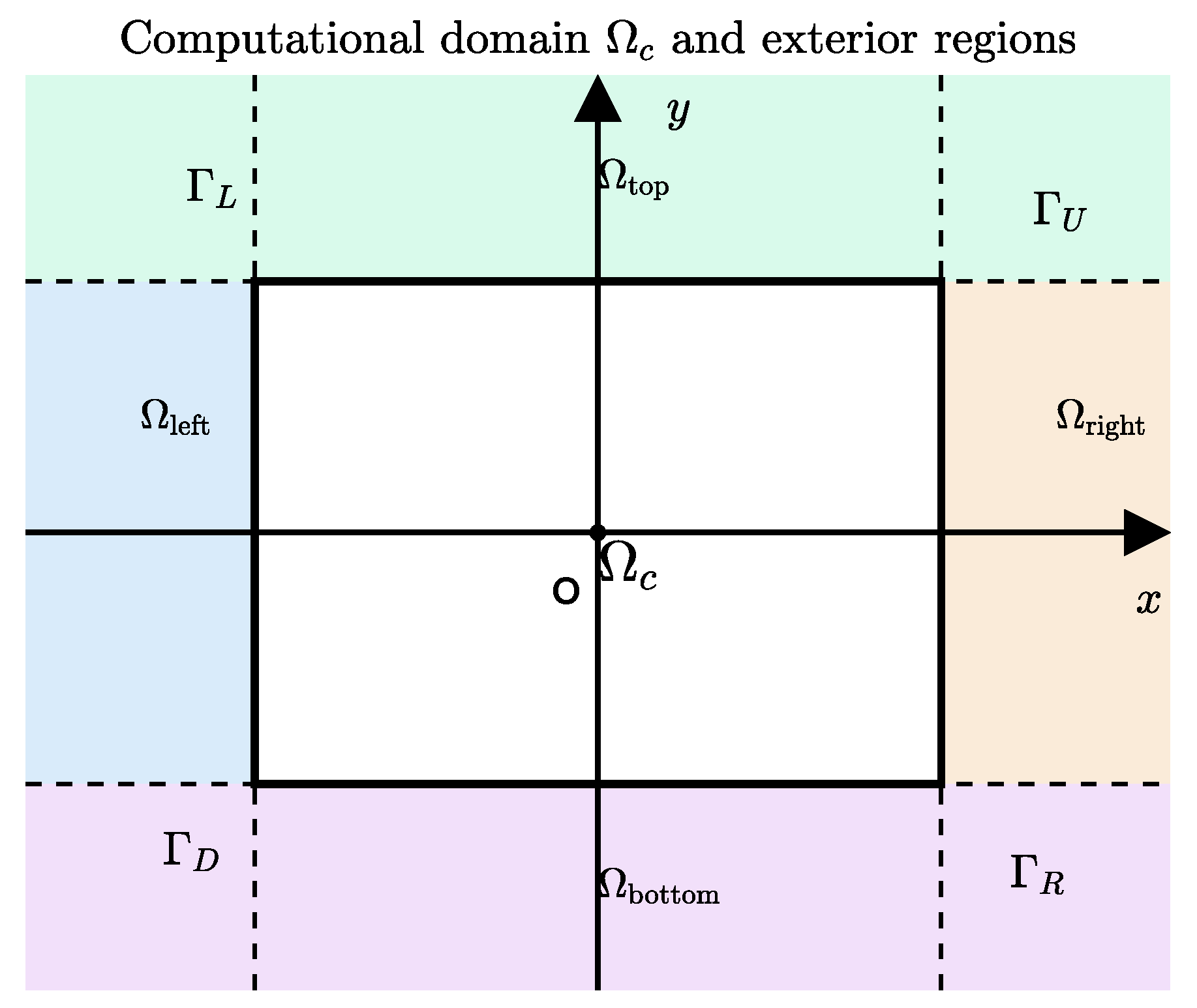
The computational domain is defined as the rectangular region Ω c = [ x l , x r ] × [ y b , y t ] . As illustrated in Figure 1, the truncation divides the original unbounded domain into the interior Ω c and four exterior regions:
Ω right = { ( x , y ) x > x r , y b < y < y t } , Ω left = { ( x , y ) x < x l , y b < y < y t } , Ω top = { ( x , y ) x l < x < x r , y > y t } , Ω bottom = { ( x , y ) x l < x < x r , y < y b } .
We assume that all backbone locations satisfy y b < l 1 < < l N < y t , so that the entire singular support of S ( y ) lies strictly inside Ω c . Consequently, the top and bottom exterior regions contain no backbones.
Within these exterior regions, the backbone structure extends outward, maintaining the structural distribution S ( y ) defined in (4). The problem in the exterior is governed by the source-free equation:
D t α C P ( x , y , t ) j = 1 N w j δ ( y l j ) 2 P ( x , y , t ) x 2 2 P ( x , y , t ) y 2 = 0 , ( x , y ) R 2 Ω c ,
the initial distribution is defined as a point source P 0 ( x , y ) = δ ( x , y ) centered at the origin. Since the support of P 0 is entirely contained within the computational domain Ω c , the initial density vanishes identically in the exterior region, i.e., P ( x , y , 0 ) = 0 for ( x , y ) Ω c , and far-field radiation conditions:
lim | x | P ( x , y , t ) = 0 , lim | y | P ( x , y , t ) = 0 .

2.2. Derivation via Laplace Transform

We derive the ABCs by applying the Laplace transform with respect to time, P ^ ( x , y , s ) = 0 e s t P ( x , y , t ) d t . The governing Equation (5) transforms to
s α P ^ ( x , y , s ) S ( y ) 2 P ^ x 2 2 P ^ y 2 = 0 ,
where S ( y ) = j = 1 N w j δ ( y l j ) . We now solve this elliptic problem analytically in each exterior subdomain.

2.2.1. Longitudinal Boundaries ( x = x l and x = x r )

We first consider the right exterior domain x > x r . To obtain a tractable analytic expression, we adopt a decoupled-backbone approximation, which treats the dynamics on each backbone y = l k independently. This approximation is formally justified when the characteristic transverse diffusion length between backbones is small compared to their separation, or when the weights { w k } exhibit strong heterogeneity.
To quantify the validity of this approximation, let d j k = | l j l k | denote the separation between backbones j and k. In the Laplace domain, the transverse Green’s function (resolvent) exhibits exponential attenuation exp ( s α / 2 | y l j | ) . Consequently, the contribution of backbone j to the trace on backbone k is suppressed by the factor exp ( d j k s α / 2 ) relative to the self-contribution. We define the dimensionless coupling parameter
ε k ( s ) : = j k w j w k exp d j k s α / 2 ,
which quantifies the relative magnitude of inter-backbone coupling neglected by the decoupled approximation. When ε k ( s ) 1 for all dominant Laplace frequencies s contributing to the time interval [ 0 , T ] , the off-diagonal terms in the Dirichlet-to-Neumann (DtN) operator are negligible, and the error incurred by the diagonal approximation (10) is bounded by max k ε k ( s ) .
Translating this criterion to the time domain using the characteristic transverse diffusion length ( t ) t α / 2 , the condition ε k 1 is equivalent to requiring that the minimum backbone separation d min = min j k d j k satisfies
d min ( T ) T α / 2 ,
or, in terms of a characteristic crossover time, T t c where t c d min 2 / α .
Conversely, when the backbone separation is comparable to the transverse diffusion length, i.e., d j k O ( ( t ) ) for some t T (equivalently d j k s α / 2 = O ( 1 ) in Laplace variables), transverse exchange between backbones is no longer negligible. In this regime, the exact DtN operator becomes coupled (non-diagonal) in the backbone index k, and the relations derived below should be interpreted as a leading-order diagonal approximation whose accuracy degrades as d j k approaches ( T ) .
Proceeding under the decoupled approximation, we focus on the line y = l k where the distributional term δ ( y l k ) induces a jump in the transverse derivative. Integrating (6) across an infinitesimal interval around y = l k yields the jump condition:
P ^ y l k l k + = w k 2 P ^ x 2 ( x , l k , s ) .
Away from the backbones, the solution satisfies the modified Helmholtz equation s α P ^ 2 P ^ y 2 = 0 . To isolate the dominant contribution from the k-th backbone, we employ the free-space Green’s function identity:
2 y 2 e s α / 2 | y l k | = s α e s α / 2 | y l k | 2 s α / 2 δ ( y l k ) .
Substituting the ansatz P ^ ( x , y , s ) ϕ k ( x , s ) e s α / 2 | y l k | into (6) and matching coefficients of δ ( y l k ) , we obtain an ordinary differential equation for the trace ϕ k ( x , s ) = P ^ ( x , l k , s ) :
d 2 ϕ k d x 2 = 2 s α / 2 w k ϕ k .
The general solution is ϕ k ( x , s ) = A k ( s ) e 2 w k s α / 4 x + B k ( s ) e + 2 w k s α / 4 x . Boundedness as x + requires B k ( s ) = 0 . Thus, for x x r ,
P ^ ( x , l k , s ) = P ^ ( x r , l k , s ) exp 2 w k s α / 4 ( x x r ) .
Differentiating and evaluating at x = x r yields the Dirichlet-to-Neumann (DtN) map:
P ^ ( x r , l k , s ) x = 2 w k s α / 4 P ^ ( x r , l k , s ) , k = 1 , , N .
By symmetry, in the left exterior domain ( x < x l ), boundedness as x selects the decaying exponential (in the negative direction), leading to:
P ^ ( x l , l k , s ) x = 2 w k s α / 4 P ^ ( x l , l k , s ) , k = 1 , , N .
Remark 1.
The longitudinal DtN relations (10) and (11) are exact for the diagonalized exterior model obtained under the decoupled-backbone approximation. For the original multi-backbone problem, they constitute a leading-order asymptotic approximation. The quantitative validity is governed by the dimensionless parameter ε k ( s ) defined in (7): when max k ε k ( s ) 1 over the Laplace frequencies relevant to the simulation window [ 0 , T ] , the diagonal approximation is accurate with relative error O ( ε ) . When the backbone separation d j k becomes comparable to the transverse fractional diffusion length ( T ) T α / 2 , the coupling parameter ε k approaches unity, and the exact DtN operator must account for off-diagonal (inter-backbone) coupling terms.

2.2.2. Transverse Boundaries ( y = y b and y = y t )

In the top exterior region ( y > y t ), no backbones are present ( S ( y ) 0 ), so (6) reduces to
s α P ^ 2 P ^ y 2 = 0 .
The decaying solution as y + is P ^ ( x , y , s ) = P ^ ( x , y t , s ) e s α / 2 ( y y t ) , which implies
P ^ ( x , y t , s ) y = s α / 2 P ^ ( x , y t , s ) .
Similarly, for the bottom region ( y < y b ), decay as y gives
P ^ ( x , y b , s ) y = s α / 2 P ^ ( x , y b , s ) .

2.3. Time-Domain Boundary Conditions

To implement these conditions in a time-stepping scheme, we apply the inverse Laplace transform. Since the exterior solution satisfies homogeneous initial conditions ( P = 0 at t = 0 in R 2 Ω c ), the Riemann–Liouville and Caputo fractional derivatives coincide. Recalling that L { D t α C f ( t ) } = s β f ^ ( s ) for f ( 0 ) = 0 , we obtain the exact time-domain ABCs.
For the longitudinal boundaries (evaluated at each backbone y = l j ):
P ( x r , l j , t ) x = 2 w j D t α / 4 C P ( x r , l j , t ) ,
P ( x l , l j , t ) x = 2 w j D t α / 4 C P ( x l , l j , t ) .
For the transverse boundaries (valid for all x [ x l , x r ] ):
P ( x , y t , t ) y = D t α / 2 C P ( x , y t , t ) ,
P ( x , y b , t ) y = D t α / 2 C P ( x , y b , t ) .
Remark 2.
For the special case of a single backbone ( N = 1 , w 1 = 1 , l 1 = 0 ), our derived conditions (15)–(18) exactly recover the results of Liu et al. [18]. The key generalization here is the factor 2 w j , which explicitly encodes the influence of the structural weight on the escape rate: backbones with larger w j act as more efficient conduits for particle outflow.

2.4. Summary of Interior and Boundary Stencils

Below is a Table 1 summarizing the interior and boundary stencils for the discretization scheme.
The derived ABCs reveal a fundamental anisotropy in particle escape mechanisms. On the transverse boundaries (Top/Bottom), the boundary operator involves the derivative order α / 2 , corresponding to pure fractional diffusion in the ambient medium. In contrast, on the longitudinal boundaries (Left/Right), the derivative order is α / 4 . This significantly lower order implies a heavier-tailed memory kernel, reflecting the slower, sub-diffusive transport constrained along the backbones. The prefactor 2 w j further indicates that backbones with larger weights facilitate faster transport (lower resistance), effectively serving as primary highways for particle egress. This dual scaling, α / 2 versus α / 4 , is a direct mathematical manifestation of the geometric dichotomy between the continuous transverse space and the singular, discrete backbone network.

2.5. Analytical Solution and Asymptotic Behavior of MSD

A key observable characterizing anomalous transport is the mean-square displacement (MSD) along the longitudinal direction:
x 2 ( t ) = R 2 x 2 P ( x , y , t ) d x d y .
We consider the source-free dimensionless governing equation with N backbones:
D t α C P j = 1 N w j δ ( y l j ) 2 P x 2 2 P y 2 = 0 ,
subject to the point-source initial condition P ( x , y , 0 ) = δ ( x ) δ ( y ) , where we assume without loss of generality that the particle is released at the location of the first backbone, i.e., l 1 = 0 .
To obtain an analytical expression for the MSD, we adopt the decoupled backbone approximation, which assumes that inter-backbone coupling via transverse diffusion is negligible in the far field. This approximation is physically justified when the backbone separations { | l j l k | } j k are large compared to the characteristic transverse diffusion length ( t ) t α / 2 , or when the structural weights { w j } are highly heterogeneous, conditions consistent with those used in the derivation of the ABCs. Under this assumption, the dynamics on each backbone can be treated independently. Its regime of validity is the same as that discussed for the longitudinal DtN derivation in Remark 1.
Let P ^ ( x , y , s ) = L { P ( x , y , t ) ; s } denote the Laplace transform in time, and P ^ ˜ ( κ x , y , s ) = F x { P ^ ( x , y , s ) ; κ x } its Fourier transform in x. Applying these transforms to  (19) yields
s α P ^ ˜ s α 1 δ ( y ) + κ x 2 j = 1 N w j δ ( y l j ) P ^ ˜ 2 P ^ ˜ y 2 = 0 ,
which can be rearranged as a Helmholtz-type equation,
2 P ^ ˜ y 2 s α P ^ ˜ = s α 1 δ ( y ) + κ x 2 j = 1 N w j δ ( y l j ) P ^ ˜ .
The free-space Green’s function G s ( y ) [28] satisfying ( 2 y 2 s α ) G s ( y ) = δ ( y ) is given by
G s ( y ) = 1 2 s α / 2 e s α / 2 | y | .
Using this, the solution to  (20) can be constructed via the method of Green’s functions. The contribution from the initial condition δ ( y ) is s α 1 G s ( y ) = + s α 1 2 s α / 2 e s α / 2 | y | . The contribution from the backbone terms follows similarly, yielding
P ^ ˜ ( κ x , y , s ) = s α 1 2 s α / 2 e s α / 2 | y | + κ x 2 j = 1 N w j P ^ ˜ ( κ x , l j , s ) · e s α / 2 | y l j | 2 s α / 2 .
Note that both terms carry a positive sign, consistent with the structure of the inhomogeneous term in  (20).
The marginal probability density in Fourier–Laplace space is defined as
p ^ ˜ 1 ( κ x , s ) = P ^ ˜ ( κ x , y , s ) d y .
Integrating  (21) over y and using e s α / 2 | y l j | d y = 2 s α / 2 , we obtain
p ^ ˜ 1 ( κ x , s ) = 1 s + κ x 2 s α j = 1 N w j P ^ ˜ ( κ x , l j , s ) .
Under the decoupled backbone approximation, the value of P ^ ˜ ( κ x , l j , s ) is dominated by the response of the j-th backbone alone. For a particle initially localized at ( x , y ) = ( 0 , 0 ) (i.e., on backbone j = 1 ), the probability of finding the particle on backbone j after transverse equilibration is proportional to the survival probability attenuated by the transverse distance | l j | . Following standard arguments for fractional diffusion in the transverse direction [9], we approximate
P ^ ˜ ( 0 , l j , s ) = p ^ j ( s ) 1 s e | l j | s α / 2 .
Since the MSD depends only on the second derivative of p ^ ˜ 1 at κ x = 0 , we evaluate  (22) in the limit κ x 0 and find
x 2 ^ ( s ) = 2 p ^ ˜ 1 κ x 2 κ x = 0 = 1 s α j = 1 N w j p ^ j ( s ) 1 s α j = 1 N w j · 1 s e | l j | s α / 2 .
Thus, the Laplace-transformed MSD is
x 2 ^ ( s ) = s ( 1 + α / 2 ) j = 1 N w j e | l j | s α / 2 .
Applying the inverse Laplace transform and using the identity [4]
L 1 s ( 1 + β ) e a s γ ( t ) = t β E γ , 1 + β ( 1 ) ( a t γ ) , where E γ , δ ( 1 ) ( z ) = d d z E γ , δ ( z ) ,
we obtain the exact expression for the MSD,
x 2 ( t ) = j = 1 N w j t α / 2 E α / 2 , 1 + α / 2 ( 1 ) | l j | t α / 2 .
We now analyze the asymptotic behavior in two distinct temporal regimes, governed by the competition between the transverse diffusion length ( t ) t α / 2 and the backbone positions { l j } .
For short-time regime ( t α / 2 min j 2 | l j | ), the particle remains localized near the release backbone ( l 1 = 0 ). For j 2 , the exponential factors e | l j | s α / 2 suppress contributions in Laplace space, or equivalently, E α / 2 , 1 + α / 2 ( 1 ) ( | l j | t α / 2 ) 0 rapidly in time domain. Thus,
x 2 ( t ) w 1 t α / 2 E α / 2 , 1 + α / 2 ( 1 ) ( 0 ) = w 1 t α / 2 Γ ( 1 + α / 2 ) ,
where we used E γ , δ ( 1 ) ( 0 ) = 1 / Γ ( δ ) for δ > 1 . This reveals that the short-time subdiffusion is explicitly modulated by the weight w 1 of the release backbone. To clarify the connection with the classical comb model, we further consider the limiting case α = 1 in the asymptotic expressions of the MSD. Noting that Γ ( 1 + α / 2 ) | α = 1 = Γ ( 3 / 2 ) = π / 2 , one obtains the subdiffusive scaling
x 2 ( t ) t 1 / 2 Γ ( 3 / 2 ) = 2 π t 1 / 2 .
Moreover, in the backbone-dominated short-time regime
x 2 ( t ) w 1 2 π t 1 / 2 .
Therefore, the present asymptotic results recover the standard t 1 / 2 subdiffusive scaling of the classical comb model in the case α = 1 .
For long-time regime ( t α / 2 max j | l j | ), transverse equilibration is complete, and all exponential attenuation factors approach unity: e | l j | s α / 2 1 . Using the normalization j = 1 N w j = 1 , we recover the universal comb asymptotics:
x 2 ( t ) t α / 2 Γ ( 1 + α / 2 ) .
Therefore, the MSD exhibits a crossover from a weighted short-time subdiffusive regime, governed by the local backbone structure, to a universal long-time scaling independent of the specific backbone configuration. The transition occurs on the timescale t c ( min j 2 | l j | ) 2 / α , reflecting the intrinsic coupling between spatial heterogeneity and memory effects in fractal-inspired media.

3. Stability Analysis of the Truncated Problem

Having derived the exact ABCs in Section 2, we now establish the well-posedness of the associated Laplace-domain variational problem on the finite computational domain Ω c = [ x l , x r ] × [ y b , y t ] . By combining a variational argument with Laplace-domain energy estimates, we prove existence, uniqueness, and continuous dependence on the initial data and source term, thereby showing that the artificial boundaries do not introduce spurious instabilities.

3.1. Energy Estimates and Dissipativity

We consider the truncated problem in the Laplace domain, where the solution P ^ ( · , s ) (with s C , Re ( s ) > 0 ) satisfies
s α P ^ j = 1 N w j δ ( y l j ) 2 P ^ x 2 2 P ^ y 2 = s α 1 P 0 ( x , y ) + R ^ ( x , y , s ) , in Ω c ,
subject to the exact ABCs (10)–(14). To make the singular backbone operator rigorous, we pose the Laplace-domain problem in a variational framework for each fixed s C with ( s ) > 0 . We introduce the energy space
V : = v L 2 ( Ω c ) : y v L 2 ( Ω c ) and v ( · , l j ) H 1 ( x l , x r ) for j = 1 , , N ,
equipped with the norm
v V 2 : = v L 2 ( Ω c ) 2 + y v L 2 ( Ω c ) 2 + j = 1 N w j x v ( · , l j ) L 2 ( x l , x r ) 2 .
Here, v denotes a generic element of the solution/test space V (not an additional unknown). In particular, the trace mappings v v ( · , y b ) and v v ( · , y t ) are well-defined in L 2 ( x l , x r ) by the standard one-dimensional trace theorem in the y-direction, and for each backbone level l j , the trace v ( · , l j ) is an H 1 ( x l , x r ) function so that the point values v ( x l , l j ) and v ( x r , l j ) are well-defined. The singular backbone term j = 1 N w j δ ( y l j ) x 2 v is understood only in the weak sense and is rigorously represented in the variational formulation through the sesquilinear form introduced below, rather than as an L 2 ( Ω c ) function.
Let · denote the norm in L 2 ( Ω c ) , and let ( · , · ) L 2 ( Ω c ) denote the corresponding inner product. The singular backbone term is paired with test functions by the duality bracket · , · V , V whenever needed.
Assume for the moment that P ^ ( · , s ) is sufficiently smooth so that the following formal identities are valid. Multiplying (27) by P ^ ¯ and integrating over Ω c yields the following formal energy identity. The rigorous weak formulation, together with the corresponding variational solution concept, is given later in Theorem 2; the same estimate is then recovered for variational solutions by density and continuity.
s α P ^ 2 j = 1 N w j δ ( y l j ) 2 P ^ x 2 , P ^ V , V 2 P ^ y 2 , P ^ L 2 ( Ω c ) = s α 1 ( P 0 , P ^ ) L 2 ( Ω c ) + ( R ^ , P ^ ) L 2 ( Ω c ) .
We next record the formal integration-by-parts identities for the spatial operators at the smooth level, in order to exhibit the dissipative structure of the truncated problem. The rigorous weak formulation is introduced later through the sesquilinear form a s ( · , · ) in Theorem 2, and the variational stability estimate is consistent with the formal identities derived below.
For the longitudinal diffusion supported on the backbone set y = l j , j = 1 , , N , we only record the formal integration-by-parts identity for sufficiently smooth functions. In the rigorous variational formulation, the backbone contribution is incorporated through the line terms in a s ( · , · ) , without introducing boundary traces of x u at x = x l , x r .
j = 1 N w j δ ( y l j ) 2 P ^ x 2 , P ^ V , V = j = 1 N w j x l x r 2 P ^ ( x , l j ) x 2 P ^ ( x , l j ) ¯ d x = j = 1 N w j x P ^ ( · , l j ) L 2 ( x l , x r ) 2 + B x .
Here, the boundary contribution arises from evaluating the antiderivative at x = x l and x = x r ,
B x = j = 1 N w j P ^ ( x l , l j ) x P ^ ( x l , l j ) ¯ P ^ ( x r , l j ) x P ^ ( x r , l j ) ¯ .
Similarly, for the transverse diffusion term, integration by parts over the full domain yields
2 P ^ y 2 , P ^ L 2 ( Ω c ) = P ^ y 2 + B y ,
with the boundary term
B y = s α / 2 x l x r | P ^ ( x , y t , s ) | 2 + | P ^ ( x , y b , s ) | 2 d x ,
which follows from the transverse ABCs (13) and (14).
For stability, we require Re ( B x ) 0 and Re ( B y ) 0 . Writing s = r e i θ with r > 0 and | θ | < π / 2 , and noting 0 < α < 1 , we have
| arg ( s α / 4 ) | = α | θ | 4 < π 8 , | arg ( s α / 2 ) | = α | θ | 2 < π 4 .
Thus, Re ( s α / 4 ) > 0 and Re ( s α / 2 ) > 0 , ensuring Re ( B x ) 0 and Re ( B y ) 0 . This confirms the exact ABCs are strictly passive and energy-absorbing [17,29].

3.2. Stability Theorem

Based on the preceding analysis, we now establish a rigorous stability result for the truncated problem in the Laplace domain. The formal energy identities derived above motivate and are consistent with the following sesquilinear formulation, which provides the precise weak notion of solution used below.
Theorem 1
(Well-posedness and Laplace-domain stability). Assume 0 < α < 1 , ( s ) > 0 , and w j 0 for j = 1 , , N . Let P 0 L 2 ( Ω c ) and let R ( · , t ) L loc 1 ( [ 0 , ) ; L 2 ( Ω c ) ) with Laplace transform R ^ ( · , s ) L 2 ( Ω c ) for every ( s ) > 0 .
For each such s, define the sesquilinear form a s : V × V C by
a s ( u , ϕ ) : = s α ( u , ϕ ) L 2 ( Ω c ) + ( y u , y ϕ ) L 2 ( Ω c ) + j = 1 N w j ( x u ( · , l j ) , x ϕ ( · , l j ) ) L 2 ( x l , x r ) + s α / 2 x l x r u ( x , y t ) ϕ ( x , y t ) ¯ + u ( x , y b ) ϕ ( x , y b ) ¯ d x + 2 s α / 4 j = 1 N w j 3 / 2 u ( x r , l j ) ϕ ( x r , l j ) ¯ + u ( x l , l j ) ϕ ( x l , l j ) ¯ ,
and the antilinear functional F s : V C by
F s ( ϕ ) : = s α 1 ( P 0 , ϕ ) L 2 ( Ω c ) + ( R ^ ( · , s ) , ϕ ) L 2 ( Ω c ) .
Then there exists a unique P ^ ( · , s ) V such that
a s ( P ^ , ϕ ) = F s ( ϕ ) , ϕ V .
Moreover, the solution satisfies the resolvent estimate
P ^ ( · , s ) L 2 ( Ω c ) C α | s | 1 P 0 L 2 ( Ω c ) + | s | α R ^ ( · , s ) L 2 ( Ω c ) ,
where C α = cos ( α π / 2 ) 1 > 0 depends only on α.
Proof. 
By Cauchy–Schwarz, the bulk terms in a s are bounded by u V ϕ V . The boundary terms are bounded using standard one-dimensional trace inequalities in the y-direction,
v ( · , y b ) L 2 ( x l , x r ) 2 + v ( · , y t ) L 2 ( x l , x r ) 2 C tr v L 2 ( Ω c ) 2 + y v L 2 ( Ω c ) 2 ,
and the fact that v ( · , l j ) H 1 ( x l , x r ) implies the endpoint values v ( x l , l j ) , v ( x r , l j ) are well-defined and satisfy
| v ( x l , l j ) | 2 + | v ( x r , l j ) | 2 C end v ( · , l j ) H 1 ( x l , x r ) 2 .
Moreover, by the one-dimensional trace inequality in the y-direction,
v ( · , l j ) L 2 ( x l , x r ) 2 C j v L 2 ( Ω c ) 2 + y v L 2 ( Ω c ) 2 .
Hence,
v ( · , l j ) H 1 ( x l , x r ) 2 C v L 2 ( Ω c ) 2 + y v L 2 ( Ω c ) 2 + x v ( · , l j ) L 2 ( x l , x r ) 2 C v V 2 ,
so that the endpoint values v ( x l , l j ) and v ( x r , l j ) are controlled by v V . Consequently, for each fixed s with ( s ) > 0 there exists a constant M s > 0 (depending on s, Ω c , and { w j } ) such that
| a s ( u , ϕ ) | M s u V ϕ V , u , ϕ V .
Similarly, F s is bounded on V since
| ( P 0 , ϕ ) L 2 ( Ω c ) | P 0 L 2 ( Ω c ) ϕ L 2 ( Ω c ) P 0 L 2 ( Ω c ) ϕ V ,
and likewise for R ^ .
Taking ϕ = u and real parts, and using ( s α / 4 ) > 0 , ( s α / 2 ) > 0 , we obtain
a s ( u , u ) = ( s α ) u L 2 ( Ω c ) 2 + y u L 2 ( Ω c ) 2 + j = 1 N w j x u ( · , l j ) L 2 ( x l , x r ) 2 + ( s α / 2 ) u ( · , y t ) L 2 ( x l , x r ) 2 + u ( · , y b ) L 2 ( x l , x r ) 2 + 2 ( s α / 4 ) j = 1 N w j 3 / 2 | u ( x r , l j ) | 2 + | u ( x l , l j ) | 2 min { ( s α ) , 1 } u V 2 .
Hence, a s is coercive on V for every ( s ) > 0 .
By the boundedness and coercivity established above, the complex Lax–Milgram theorem yields a unique P ^ ( · , s ) V solving the variational problem (31) for each fixed s with ( s ) > 0 .
Choosing ϕ = P ^ in (31) and taking real parts gives
( s α ) P ^ L 2 ( Ω c ) 2 | s | α 1 P 0 L 2 ( Ω c ) P ^ L 2 ( Ω c ) + R ^ L 2 ( Ω c ) P ^ L 2 ( Ω c ) ,
after discarding the nonnegative backbone, gradient, and boundary contributions (these correspond exactly to the dissipative terms displayed in (29) and (30)). For P ^ L 2 ( Ω c ) > 0 , divide both sides by P ^ L 2 ( Ω c ) to obtain
( s α ) P ^ L 2 ( Ω c ) | s | α 1 P 0 L 2 ( Ω c ) + R ^ L 2 ( Ω c ) .
Finally, since ( s α ) cos ( α π / 2 ) | s | α for ( s ) > 0 , we deduce (32) with C α = ( cos ( α π / 2 ) ) 1 .
Uniqueness also follows directly from (32): if P 0 = 0 and R ^ ( · , s ) = 0 , then P ^ ( · , s ) L 2 ( Ω c ) = 0 , hence P ^ ( · , s ) 0 .    □
The stability constant C α = ( cos ( α π / 2 ) ) 1 in (32) is independent of the backbone weights { w j } , reflecting the fact that larger w j only enhances dissipation through the backbone term j w j x P ^ ( · , l j ) 2 and the longitudinal boundary flux B x j w j 3 / 2 | P ^ | 2 in (29). Specifically, the resolvent bound depends on the weights only through the aggregated measure w max = max j w j in the sense that P ^ decreases monotonically as w j increases, but the bounding constant C α need not increase. For the discrete scheme, this translates to stability constants that are robust with respect to variations in the structural weights, provided the Courant-type condition implicit in the fractional CFL number is satisfied (see Section 4.5).
In the source-free case ( R 0 , hence R ^ = 0 ), the Laplace-domain stability estimate (32) implies uniform boundedness of the physical solution in time. Specifically, under the standard assumptions that P ^ ( · , s ) is analytic in the right half-plane { s C : Re ( s ) > 0 } and satisfies a mild growth condition (e.g., P ^ ( · , s ) L 2 ( Ω c ) = O ( | s | 1 ) as | s | within any sector | arg s | π / 2 ε ), classical Tauberian-type arguments for the inverse Laplace transform [29], yield the following uniform-in-time energy bound.
Assume R 0 and P 0 L 2 ( Ω c ) . Then the solution P ( · , t ) of the truncated initial-boundary value problem with exact ABCs satisfies
P ( · , t ) L 2 ( Ω c ) C ˜ P 0 L 2 ( Ω c ) , t > 0 ,
where the constant C ˜ > 0 depends only on the fractional order α , the domain geometry Ω c , and the backbone weights { w j } j = 1 N , but is independent of time t and the initial data P 0 .
Remark 3.
The Laplace-domain stability estimate (32) relies fundamentally on the non-negativity of (i) the backbone dissipation j = 1 N w j x P ^ ( · , l j ) L 2 2 and (ii) the boundary flux contributions Re ( B x ) , Re ( B y ) from (29) to (30).
In the fully discrete scheme presented in Section 4.5, these structural properties are preserved exactly: discrete summation-by-parts yields the analogous weighted backbone dissipation, while the discrete ABCs generate boundary flux terms with identical dissipative signs. Consequently, the discrete solution satisfies a stability bound consistent with (32), namely
P n 2 C α P 0 2 + C α Δ t α k = 0 n 1 R k 2 ,
where the constant C α remains independent of the time step Δ t and mesh size h, ensuring unconditional stability and asymptotic preservation of the continuous energy dissipation structure.
This result confirms that the artificial boundaries equipped with the derived exact absorbing conditions do not introduce spurious energy growth, thereby ensuring the Laplace-domain well-posedness and supporting the subsequent discrete stability analysis.

4. Finite Difference Discretization

This section is devoted to the construction of a fully discrete scheme for solving the initial-boundary value problem governed by (4) on the bounded computational domain Ω c = [ x l , x r ] × [ y b , y t ] . The discretization addresses two principal challenges: the non-local temporal memory inherent in the Caputo fractional derivative and the spatial singularity introduced by the Dirac delta distribution S ( y ) = j = 1 N w j δ ( y l j ) representing the backbones. We propose a hybrid approach that combines the L1 finite difference scheme for the temporal operator with a finite volume integration technique in the transverse direction to rigorously handle the geometric constraints [30].

4.1. Mesh Partition and Notation

A uniform temporal mesh is introduced over the time interval [ 0 , T ] with step size τ = T / N t , defining time levels t n = n τ for n = 0 , 1 , , N t . The spatial domain Ω c is discretized using uniform grids:
(1)
For the x-direction, mesh size h x = ( x r x l ) / M x , with grid points x i = x l + i h x for i = 0 , 1 , , M x .
(2)
For the y-direction, mesh size h y = ( y t y b ) / M y , with grid points y k = y b + k h y for k = 0 , 1 , , M y .
To evaluate the singular backbone contribution exactly on the present mesh, we assume that each backbone location l j ( j = 1 , , N ) coincides with a transverse grid line. Specifically, for each j, there exists a unique index k j { 1 , , M y 1 } such that
y k j = l j , j = 1 , 2 , , N .
Under this alignment, the finite-volume integrals involving the Dirac comb j = 1 N w j δ ( y l j ) can be evaluated exactly.
Let P i , k n denote the numerical approximation to P ( x i , y k , t n ) . We define standard second-order central difference operators,
δ x 2 P i , k n = P i + 1 , k n 2 P i , k n + P i 1 , k n h x 2 , δ y 2 P i , k n = P i , k + 1 n 2 P i , k n + P i , k 1 n h y 2 .

4.2. Treatment of the Singular Structure via Finite Volume Integration

The presence of the Dirac measure S ( y ) in  (4) renders pointwise evaluation of the governing equation ill-defined at backbone locations. To circumvent this singularity while preserving physical consistency, we adopt a finite volume approach: the equation is integrated over a transverse control volume centered at each grid point y k , namely the interval [ y k 1 / 2 , y k + 1 / 2 ] with y k ± 1 / 2 = y k ± h y / 2 . This yields
y k 1 / 2 y k + 1 / 2 D t α C P S ( y ) 2 P x 2 2 P y 2 d y = y k 1 / 2 y k + 1 / 2 R ( x , y , t ) d y .
This formulation enforces local conservation of mass across each transverse slab—a critical property for accurately capturing transport dynamics on singular (measure-supported) geometries.

4.2.1. Discretization of Regular Terms

The regular terms in  (34) are approximated using the midpoint rule, which provides second-order accuracy in space,
y k 1 / 2 y k + 1 / 2 D t α C P ( x , y , t ) d y h y D t α C P ( x , y k , t ) , y k 1 / 2 y k + 1 / 2 y 2 P ( x , y , t ) d y h y δ y 2 P ( x i , y k , t ) ,
where δ y 2 denotes the standard second-order central difference operator in the y-direction. For consistency, we denote the cell-averaged source term by
R i , k ( t ) : = 1 h y y k 1 / 2 y k + 1 / 2 R ( x i , y , t ) d y .

4.2.2. Discretization of the Singular Backbone Term

For the singular term involving S ( y ) , each backbone location l j coincides exactly with a grid point y k j . Leveraging the sifting property of the Dirac measure, we obtain
y k 1 / 2 y k + 1 / 2 S ( y ) 2 P ( x , y , t ) x 2 d y = j = 1 N w j δ k , k j 2 P ( x , l j , t ) x 2 .
Here, w j represents the strength (or weight) associated with the j-th backbone, and δ k , k j is the Kronecker delta enforcing localization at the aligned grid index.
Dividing (34) by the cell width h y and substituting the above approximations leads to the semi-discrete scheme
D t α C P i , k j = 1 N w j h y δ k , k j δ x 2 P i , k δ y 2 P i , k = R i , k + O ( h x 2 + h y 2 ) ,
where R i , k denotes the cell-averaged source term. The factor w j / h y appears because the singular backbone contribution is obtained by integrating a line-supported measure over a transverse control volume and then normalizing by the cell width.
Table 2 summarizes the finite-volume stencils employed across the interior domain, the singular backbones, and the artificial boundaries equipped with exact ABCs, detailing the spatial discretization and convergence order for each region.

4.3. Boundary Treatment and Ghost-Point Formulation

To implement the exact ABCs (11)–(14) on the discrete level, we employ a ghost-point approach where the Dirichlet-to-Neumann relations are enforced at grid points x 0 = x l and x M x = x r (longitudinal) and y 0 = y b , y M y = y t (transverse). This requires computing the fractional convolution histories at each boundary node and solving for the ghost values P 1 , k n and P M x + 1 , k n .
The numerical realization of the exact ABCs via the ghost-point method involves evaluating fractional convolution histories at boundary nodes and solving for ghost values using the DtN maps; the detailed procedure is summarized in Algorithm 1.
Remark 4.
The grid-alignment condition (33) is imposed only to evaluate the singular backbone contribution exactly on the given mesh. If a backbone location l j does not coincide with a grid line, one may replace the distribution δ ( y l j ) by a conservative two-point discrete projection in the transverse direction.
Assume that l j ( y k , y k + 1 ) for some k, and define
θ j : = l j y k h y ( 0 , 1 ) .
We then introduce the discrete measure
δ h , j : = ( 1 θ j ) δ y k + θ j δ y k + 1 ,
where δ y k and δ y k + 1 denote the Dirac measures supported at y k and y k + 1 , respectively. This approximation is conservative in the sense that
δ h , j , 1 = 1 ,
and, for every test function ϕ C 2 ( [ y b , y t ] ) ,
δ ( · l j ) δ h , j , ϕ = ϕ ( l j ) ( 1 θ j ) ϕ ( y k ) + θ j ϕ ( y k + 1 ) = O ( h y 2 ) .
Hence, in weak form,
δ ( y l j ) x 2 P δ h , j ( y ) x 2 P ,
which yields the second-order consistent replacement
1 h y y m 1 / 2 y m + 1 / 2 δ ( y l j ) x 2 P ( x , y , t ) d y 1 θ j h y x 2 P ( x , y k , t ) , m = k , θ j h y x 2 P ( x , y k + 1 , t ) , m = k + 1 , 0 , otherwise .
Accordingly, after division by h y , the backbone contribution in the semi-discrete scheme is distributed to the two neighboring transverse rows with coefficients
w j ( 1 θ j ) h y and w j θ j h y .
This modification preserves the total backbone mass, remains compatible with the subsequent L1 time discretization and boundary treatment, and reduces to (35) when l j is aligned with a grid line.
Algorithm 1 Ghost-point implementation of exact ABCs
 1:
Input: Solution arrays { P i , k n } for i = 0 , , M x , k = 0 , , M y at time t n ; history kernels { K long m } m = 0 n , { K trans m } m = 0 n
 2:
Output: Ghost values P 1 , k n , P M x + 1 , k n (longitudinal) and P i , 1 n , P i , M y + 1 n (transverse)
 3:
Longitudinal boundaries ( x = x l and x = x r ):
 4:
for each backbone j = 1 , , N at y = y k j  do
 5:
   Compute convolution history at x = x l :
 6:
       H l , j n m = 0 n 1 K long n m ( P 0 , k j m + P 1 , k j m )
 7:
   Solve for ghost value using DtN map (11):
 8:
       P 1 , k j n P 1 , k j n 2 h x = 2 w j m = 0 n K long n m P 0 , k j m
 9:
   Analogous for x = x r with sign reversed
10:
end for
11:
Transverse boundaries ( y = y b and y = y t ):
12:
for each i = 1 , , M x 1  do
13:
   Compute fractional integral history:
14:
       Φ b , i n m = 0 n K trans n m P i , 0 m
15:
   Apply Neumann condition (14):
16:
       P i , 1 n P i , 1 n 2 h y = Φ b , i n
17:
   Analogous for y = y t
18:
end for
19:
return Ghost values for next time step computation

4.4. Temporal Discretization: L1 Approximation

To discretize the Caputo fractional derivative D t α C P ( t ) in time, we employ the well-established L1 scheme [31]. Let t n = n τ for n = 0 , 1 , , N t , with uniform time step τ > 0 . The L1 approximation at time t n is given by
D τ α P n : = τ α Γ ( 2 α ) a 0 ( α ) P n m = 1 n 1 ( a n m 1 ( α ) a n m ( α ) ) P m a n 1 ( α ) P 0 ,
where the coefficients are defined as a k ( α ) = ( k + 1 ) 1 α k 1 α for k 0 . The sequence { a k ( α ) } k = 0 is positive, strictly decreasing, and convex—properties that are instrumental in establishing energy stability for the fully discrete system. Moreover, if P C 2 ( [ 0 , T ] ) , the local truncation error of the L1 scheme is O ( τ 2 α ) [23]. For later use in the boundary discretization, we employ the same L1 formula for any fractional order β { α , α / 2 , α / 4 } and write
D τ β P n : = τ β Γ ( 2 β ) a 0 ( β ) P n m = 1 n 1 a n m 1 ( β ) a n m ( β ) P m a n 1 ( β ) P 0 ,
where a k ( β ) = ( k + 1 ) 1 β k 1 β for k 0 . In particular, the operators D τ α / 2 and D τ α / 4 are used below for the transverse and longitudinal absorbing boundary conditions, respectively.

4.5. Boundary Discretization and Fully Discrete System

We now discretize the exact absorbing boundary conditions derived in Section 2 by the ghost-point method. The key point is that the longitudinal ABCs act only at the backbone endpoints ( x l , l j ) and ( x r , l j ) , whereas the transverse ABCs act on the top and bottom edges y = y t and y = y b . Since all backbone locations satisfy y b < l j < y t , no backbone intersects the top or bottom boundary. Consequently, the singular longitudinal diffusion term is absent at k = 0 and k = M y .
  • Longitudinal boundaries at backbone endpoints.
Consider first the right boundary x = x r at the backbone node ( x M x , y k j ) . From (15),
P ( x r , l j , t ) x = 2 w j D t α / 4 C P ( x r , l j , t ) .
Using a ghost value P M x + 1 , k j n and the central approximation of the normal derivative gives
P M x + 1 , k j n P M x 1 , k j n 2 h x = 2 w j D τ α / 4 P M x , k j n ,
hence,
P M x + 1 , k j n = P M x 1 , k j n 2 h x 2 w j D τ α / 4 P M x , k j n .
Substituting this ghost value into the second-order stencil yields
δ x 2 P M x , k j n = 2 ( P M x 1 , k j n P M x , k j n ) h x 2 2 2 w j h x D τ α / 4 P M x , k j n .
Therefore, the discrete equation at the right backbone endpoint is
D τ α P M x , k j n w j h y 2 ( P M x 1 , k j n P M x , k j n ) h x 2 2 2 w j h x D τ α / 4 P M x , k j n δ y 2 P M x , k j n = R M x , k j n .
Similarly, at the left boundary x = x l , (16) gives
P ( x l , l j , t ) x = 2 w j D t α / 4 C P ( x l , l j , t ) .
Using a ghost value P 1 , k j n and the central approximation,
P 1 , k j n P 1 , k j n 2 h x = 2 w j D τ α / 4 P 0 , k j n ,
we obtain
P 1 , k j n = P 1 , k j n 2 h x 2 w j D τ α / 4 P 0 , k j n ,
and hence,
δ x 2 P 0 , k j n = 2 ( P 1 , k j n P 0 , k j n ) h x 2 2 2 w j h x D τ α / 4 P 0 , k j n .
Thus the discrete equation at the left backbone endpoint is
D τ α P 0 , k j n w j h y 2 ( P 1 , k j n P 0 , k j n ) h x 2 2 2 w j h x D τ α / 4 P 0 , k j n δ y 2 P 0 , k j n = R 0 , k j n .
Transverse boundaries.
Since S ( y ) = 0 on y = y t and y = y b , the governing equation on the top and bottom edges contains no longitudinal diffusion term. At the top boundary, (17) gives
P ( x , y t , t ) y = D t α / 2 C P ( x , y t , t ) .
Introducing the ghost value P i , M y + 1 n and using the central approximation,
P i , M y + 1 n P i , M y 1 n 2 h y = D τ α / 2 P i , M y n ,
we obtain
P i , M y + 1 n = P i , M y 1 n 2 h y D τ α / 2 P i , M y n ,
and therefore,
δ y 2 P i , M y n = 2 ( P i , M y 1 n P i , M y n ) h y 2 2 h y D τ α / 2 P i , M y n .
Hence, the discrete top-boundary equation is
D τ α P i , M y n 2 ( P i , M y 1 n P i , M y n ) h y 2 2 h y D τ α / 2 P i , M y n = R i , M y n , 0 i M x .
At the bottom boundary, (18) gives
P ( x , y b , t ) y = D t α / 2 C P ( x , y b , t ) .
Using the ghost value P i , 1 n ,
P i , 1 n P i , 1 n 2 h y = D τ α / 2 P i , 0 n ,
we obtain
P i , 1 n = P i , 1 n 2 h y D τ α / 2 P i , 0 n ,
and thus
δ y 2 P i , 0 n = 2 ( P i , 1 n P i , 0 n ) h y 2 2 h y D τ α / 2 P i , 0 n .
Therefore, the discrete bottom-boundary equation is
D τ α P i , 0 n 2 ( P i , 1 n P i , 0 n ) h y 2 2 h y D τ α / 2 P i , 0 n = R i , 0 n , 0 i M x .
Interior equations.
For later reference, the interior scheme takes the form
D τ α P i , k n δ y 2 P i , k n = R i , k n , 1 i M x 1 , 1 k M y 1 , k { k 1 , , k N } ,
and, on the backbone rows,
D τ α P i , k j n w j h y δ x 2 P i , k j n δ y 2 P i , k j n = R i , k j n , 1 i M x 1 , j = 1 , , N .
At each time level t n , the unknown vector P n = { P i , k n } is obtained from a linear system whose matrix consists of the interior finite-difference operator together with the above ghost-point boundary closures. The right-hand side contains the source term and the L1 history contributions from previous time levels.
Remark 5.
For numerical simulations with the point-source initial condition P ( x , y , 0 ) = δ ( x ) δ ( y ) , we use the mass-preserving discrete approximation
P i , k 0 = δ i , i 0 δ k , k 0 h x h y ,
where ( x i 0 , y k 0 ) is the grid point nearest to the source location. This choice satisfies
i = 0 M x k = 0 M y P i , k 0 h x h y = 1 .
The stability and convergence analysis in Section 5, however, is carried out under the standard assumption that the initial data belongs to L 2 ( Ω c ) (and, for the convergence estimate, to a smoother class). Thus, the discrete delta initial condition used in the simulations is not covered directly by the present energy argument. A common interpretation is to approximate the Dirac mass by a family of smooth mollifiers P 0 ( ε ) L 2 ( Ω c ) with unit mass and P 0 ( ε ) δ weakly as ε 0 . This provides a consistent regularization viewpoint for the numerical initialization, but a complete convergence theory for measure-valued initial data is beyond the scope of the present paper. In Section 7, we therefore complement the analysis by numerical tests showing that the scheme remains stable and accurate for sharply localized initial data.

4.6. Algorithmic Summary of Boundary Treatment

For each time level t n , the boundary treatment is implemented as follows.
1.
Compute the L1 history terms for the three fractional orders that appear in the scheme: D τ α in the interior equation, D τ α / 4 at the longitudinal backbone endpoints, and D τ α / 2 on the transverse boundaries.
2.
Update all interior non-backbone nodes by (45) and all interior backbone nodes by (46).
3.
For each backbone level k j , impose the longitudinal absorbing boundary conditions at ( 0 , k j ) and ( M x , k j ) through the ghost-point relations associated with (42) and (41).
4.
For each i = 0 , , M x , impose the transverse absorbing boundary conditions at ( i , 0 ) and ( i , M y ) through the ghost-point relations associated with (44) and (43).
5.
Assemble the resulting linear system for the unknown vector P n and solve for the solution at the current time level.
This summary makes explicit that the longitudinal ABCs act only at the backbone endpoints, while the transverse ABCs act on the full top and bottom edges.

5. Stability and Convergence of the Fully Discrete Scheme

In this section, we establish the stability and convergence of the finite difference scheme developed in Section 4. The analysis incorporates the specific features of the Comb model, including the singular backbone term and the non-local ABCs. A distinctive feature of our analysis is the rigorous treatment of boundary conditions via the ghost point method, which ensures that the scheme maintains global second-order spatial accuracy [17].
The ghost-point boundary formulas (41)–(44) are obtained from the continuous absorbing boundary conditions (15)–(18) by combining centered normal differences with the L1 approximation of the corresponding fractional time operators. They therefore constitute a consistent discretization of the continuous DtN maps.
No additional penalty term is introduced. The discrete absorbing terms preserve the same dissipative sign as the continuous boundary fluxes; see (29), (30) and (52). Hence, the discrete boundary treatment does not generate spurious numerical growth, and its effect on long-time accuracy is accounted for by the boundary truncation error.
We assume throughout this section that the exact solution possesses sufficient regularity:
P C 2 [ 0 , T ] ; H 3 ( Ω c ) C 1 [ 0 , T ] ; H 4 ( Ω c ) .

5.1. Discrete Norms and Energy Functionals

We utilize the discrete grid function space defined on Ω h .
Definition 1.
For grid functions u = { u i , k } and v = { v i , k } , we define the discrete L 2 inner product and norm as
u , v = h x h y i = 0 M x k = 0 M y u i , k v i , k , v 2 = v , v .
Lemma 1
([23]). The L1 discretization of the Caputo derivative D τ α P n satisfies the expansion:
D τ α P n = τ α Γ ( 2 α ) a 0 ( α ) P n m = 1 n 1 ( a n m 1 ( α ) a n m ( α ) ) P m a n 1 ( α ) P 0 ,
where a j ( α ) = ( j + 1 ) 1 α j 1 α are the L1 coefficients satisfying a j ( α ) > a j + 1 ( α ) > 0 and j = 0 n 1 ( a j ( α ) a j + 1 ( α ) ) = 1 a n ( α ) .

5.2. Positivity of the L1 Operator

The following lemma is fundamental for establishing energy stability.
Lemma 2.
For any grid function sequence { v m } m = 0 n , the L1 discrete operator D τ α satisfies
v n , D τ α v n τ α 2 Γ ( 2 α ) a 0 ( α ) v n 2 2 m = 0 n 1 ( a n m 1 ( α ) a n m ( α ) ) v m 2 2 .
The same argument applies without change to D τ β for any β ( 0 , 1 ) ; in particular, it will be used below for β = α / 4 and β = α / 2 .
Proof. 
Recall the L1 discretization of the Caputo derivative at time level t n ,
D τ α v n = τ α Γ ( 2 α ) a 0 ( α ) v n m = 1 n 1 ( a n m 1 ( α ) a n m ( α ) ) v m a n 1 ( α ) v 0 ,
where a k ( α ) = ( k + 1 ) 1 α k 1 α > 0 , and the sequence { a k ( α ) } is strictly decreasing and convex.
Taking the inner product with v n , we obtain
v n , D τ α v n = τ α Γ ( 2 α ) a 0 ( α ) v n 2 2 m = 0 n 1 ( a n m 1 ( α ) a n m ( α ) ) v n , v m ,
where we set a 1 ( α ) : = a 0 ( α ) for notational consistency in the m = 0 term.
Applying the elementary inequality v n , v m 1 2 ( v n 2 2 + v m 2 2 ) , we obtain
v n , D τ α v n τ α Γ ( 2 α ) [ a 0 ( α ) v n 2 2 1 2 m = 0 n 1 ( a n m 1 ( α ) a n m ( α ) ) ( v n 2 2 + v m 2 2 ) ] = τ α 2 Γ ( 2 α ) 2 a 0 ( α ) ( a 0 ( α ) a n ( α ) ) v n 2 2 m = 0 n 1 ( a n m 1 ( α ) a n m ( α ) ) v m 2 2 = τ α 2 Γ ( 2 α ) ( a 0 ( α ) + a n ( α ) ) v n 2 2 m = 0 n 1 ( a n m 1 ( α ) a n m ( α ) ) v m 2 2 .
Since a n ( α ) > 0 , discarding this positive term yields the desired lower bound (48).    □

5.3. Discrete Integration by Parts and Boundary Dissipation

We now introduce discrete operators consistent with the fully discrete scheme in Section 4.5. In accordance with (44) and (45), we separate the boundary closures into a purely spatial part and an absorbing part.
For a grid function U n = { U i , k n } , define the purely spatial operator L h sp by
( L h sp U n ) i , k = δ y 2 U i , k n , 1 i M x 1 , 1 k M y 1 , k { k 1 , , k N } , w j h y δ x 2 U i , k j n + δ y 2 U i , k j n , 1 i M x 1 , j = 1 , , N , w j h y 2 ( U M x 1 , k j n U M x , k j n ) h x 2 + δ y 2 U M x , k j n , i = M x , k = k j , w j h y 2 ( U 1 , k j n U 0 , k j n ) h x 2 + δ y 2 U 0 , k j n , i = 0 , k = k j , 2 ( U i , M y 1 n U i , M y n ) h y 2 , k = M y , 0 i M x , 2 ( U i , 1 n U i , 0 n ) h y 2 , k = 0 , 0 i M x .
The top and bottom rows contain no δ x 2 contribution, since the singular longitudinal diffusion acts only on the backbone set y = l j with y b < l j < y t .
Next, define the absorbing operator L h abs by
( L h abs U n ) i , k = 2 2 w j 3 / 2 h x h y D τ α / 4 U M x , k j n , i = M x , k = k j , 2 2 w j 3 / 2 h x h y D τ α / 4 U 0 , k j n , i = 0 , k = k j , 2 h y D τ α / 2 U i , M y n , k = M y , 0 i M x , 2 h y D τ α / 2 U i , 0 n , k = 0 , 0 i M x , 0 , otherwise .
With these definitions, the fully discrete scheme can be written compactly as
D τ α P n L h sp P n + L h abs P n = R n .
We equip the grid functions with the discrete inner product
U , V h : = h x h y i = 0 M x k = 0 M y U i , k V i , k , U h : = U , U h .
For later use, define the discrete energy seminorm
| U n | 1 , h 2 : = h x h y i = 0 M x k = 0 M y 1 δ y + U i , k n 2 + h x j = 1 N w j i = 0 M x 1 δ x + U i , k j n 2 ,
where
δ y + U i , k n : = U i , k + 1 n U i , k n h y , δ x + U i , k j n : = U i + 1 , k j n U i , k j n h x .
Lemma 3.
For any grid function U n , the purely spatial operator L h sp satisfies
L h sp U n , U n h = | U n | 1 , h 2 0 .
Moreover, the absorbing operator satisfies
L h abs U n , U n h = 2 2 j = 1 N w j 3 / 2 U M x , k j n D τ α / 4 U M x , k j n + 2 2 j = 1 N w j 3 / 2 U 0 , k j n D τ α / 4 U 0 , k j n + 2 h x i = 0 M x U i , M y n D τ α / 2 U i , M y n + 2 h x i = 0 M x U i , 0 n D τ α / 2 U i , 0 n 0 .
Proof. 
The identity (51) follows from discrete summation-by-parts applied separately in the y-direction over all rows and in the x-direction along each backbone row. Because the longitudinal diffusion is present only on the backbone rows, the x-part contributes
h x j = 1 N w j i = 0 M x 1 δ x + U i , k j n 2 ,
while the transverse diffusion contributes
h x h y i = 0 M x k = 0 M y 1 δ y + U i , k n 2 .
The one-sided boundary closures at i = 0 , M x and k = 0 , M y are exactly those induced by the ghost-point elimination in Section 4.5, so no additional δ x 2 terms appear on the top or bottom boundaries.
For the absorbing part, the definition of L h abs together with the discrete inner product yields (52). Each term is nonnegative by Lemma 2, applied with fractional orders α / 4 and α / 2 .    □

5.4. Stability and Convergence

We now state and prove the main stability and convergence results. For clarity, we first consider the homogeneous problem ( R 0 ).
Theorem 2.
Assume the source term vanishes, i.e., R n = 0 for all n, and the initial data P 0 L 2 ( Ω c ) . Then the fully discrete scheme (49) is unconditionally stable: there exists a constant C > 0 , independent of τ, h x , and h y , such that
P n h C P 0 h , n = 1 , , N t .
Proof. 
For the homogeneous problem, (49) reads
D τ α P n L h sp P n + L h abs P n = 0 .
Taking the discrete inner product with P n gives
P n , D τ α P n h L h sp P n , P n h + L h abs P n , P n h = 0 .
By Lemma 2,
P n , D τ α P n h τ α 2 Γ ( 2 α ) a 0 ( α ) P n h 2 m = 0 n 1 a n m 1 ( α ) a n m ( α ) P m h 2 .
By Lemma 3,
L h sp P n , P n h = | P n | 1 , h 2 0 ,
and
L h abs P n , P n h 0 .
Therefore,
τ α 2 Γ ( 2 α ) a 0 ( α ) P n h 2 m = 0 n 1 a n m 1 ( α ) a n m ( α ) P m h 2 0 .
Since a 0 ( α ) = 1 and the L1 coefficients are positive and decreasing, a standard induction argument yields
P n h P 0 h , n = 1 , , N t .
This proves (53).    □
Lemma 4.
Let P ( x , y , t ) be the exact solution of the dimensionless problem (4) satisfying the regularity assumption (47). Denote by ρ i , k n the local truncation error obtained by substituting the exact solution into the fully discrete scheme at grid point ( x i , y k ) and time level t n . Then there exists a constant C > 0 , independent of τ, h x , and h y , such that
ρ n 2 C τ 2 α + h x 2 + h y 2 .
Proof. 
The local truncation error ρ i , k n is defined as the residual when the exact solution P ( x , y , t ) is inserted into the fully discrete equation,
ρ i , k n = D τ α P ( x i , y k , t n ) ( L h P ( t n ) ) i , k R ( x i , y k , t n ) .
We analyze ρ i , k n by distinguishing three types of grid points:
(i) Interior points ( i , k ) I int . At these points, the singular backbone term vanishes ( k k j for all j), and the scheme reduces to a standard central difference approximation. Under the regularity assumption (47), the Caputo derivative D t α C P is twice continuously differentiable in time, ensuring that the L1 approximation yields a temporal truncation error of O ( τ 2 α ) [23]. The second-order central differences for x 2 and y 2 contribute spatial errors of O ( h x 2 + h y 2 ) .
(ii) Backbone points ( i , k j ) with 1 i M x 1 . Here, the finite volume integration over [ y k j 1 / 2 , y k j + 1 / 2 ] exactly captures the Dirac delta contribution due to the grid-backbone alignment (33). The resulting semi-discrete Equation (36) therefore contains the longitudinal diffusion term with coefficient w j / h y on the backbone row k = k j , while the transverse part remains regular. The subsequent central difference in x thus incurs an O ( h x 2 ) error, while the y-derivative remains regular and contributes O ( h y 2 ) . The temporal error remains O ( τ 2 α ) .
(iii) Boundary points (including backbone boundaries). At the lateral boundaries ( x = x l , x r ) on backbone lines, and at the top/bottom boundaries ( y = y b , y t ), the ghost point method is employed to enforce the ABCs (15)–(18). This technique extends the central difference stencil beyond the physical domain by expressing ghost values in terms of interior values and fractional time derivatives of the boundary solution. Since the exact solution satisfies the continuous ABCs, the substitution introduces no additional leading-order error. Consequently, the spatial discretization retains second-order accuracy, i.e., O ( h x 2 ) or O ( h y 2 ) , depending on the direction. The fractional time derivatives in the ABCs are discretized using the same L1 scheme, which—by the assumed temporal regularity—contributes errors consistent with the interior, namely O ( τ 2 α ) for the main equation and O ( τ 2 α / 4 ) , O ( τ 2 α / 2 ) for the boundary fluxes. However, since 0 < α < 1 , we have 2 α / 4 > 2 α and 2 α / 2 > 2 α , so the dominant temporal error remains O ( τ 2 α ) .
Combining all contributions and noting that the number of grid points is finite, we obtain the uniform bound (55).    □
Theorem 3.
Assume the initial data P 0 H 2 ( Ω c ) is approximated by a consistent discrete projection such that e 0 2 C ( h x 2 + h y 2 ) . Let P ( x , y , t ) be the exact solution and { P i , k n } the numerical solution. Then
max 1 n N t P n P ( t n ) 2 C τ 2 α + h x 2 + h y 2 ,
where the constant C > 0 is independent of τ, h x , and h y .
Proof. 
Let e n = P n P ( t n ) denote the error. The error equation is
D τ α e n L h sp e n + L h abs e n = ρ n , n 1 ,
with e 0 2 C ( h x 2 + h y 2 ) . Taking the inner product with e n and applying Lemmas 2 and 3, we obtain
τ α 2 Γ ( 2 α ) a 0 ( α ) e n 2 2 m = 0 n 1 ( a n m 1 ( α ) a n m ( α ) ) e m 2 2 e n , ρ n .
Using Cauchy–Schwarz and Lemma 4, e n , ρ n e n 2 ρ n 2 C e n 2 ( τ 2 α + h 2 ) . A standard discrete Grönwall-type argument for fractional schemes [23] then yields
e n 2 e 0 2 + C T ( τ 2 α + h x 2 + h y 2 ) C ( τ 2 α + h x 2 + h y 2 ) ,
which completes the proof.    □
The stability and convergence results in this section are established for L 2 ( Ω c ) initial data. For the physically relevant point-source initial condition P 0 = δ ( x ) δ ( y ) , we interpret the solution through a standard regularization argument. More precisely, let { P 0 ( h ) } be a family of nonnegative Gaussian mollifiers satisfying
P 0 ( h ) ( x , y ) = 1 2 π σ h 2 exp x 2 + y 2 2 σ h 2 , σ h 0 ,
with Ω c P 0 ( h ) d x d y = 1 and P 0 ( h ) δ ( x ) δ ( y ) in the sense of distributions. For each fixed h, the above stability and convergence theory applies to the corresponding regularized problem. In the numerical experiments, we further verify that physically relevant weak observables listed in Table 3 continue to converge under this regularization.
Remark 6.
When the fast SOE algorithm is employed to accelerate the evaluation of the fractional time derivatives with a kernel approximation error ε SOE , the global error of the resulting numerical solution P fast n satisfies
P fast n P ( t n ) 2 C τ 2 α + h x 2 + h y 2 + ε SOE ,
where the constant C > 0 depends only on the final time T, the domain Ω c , and the fractional order α, but is independent of the discretization parameters τ , h x , h y and the SOE tolerance ε SOE . This estimate demonstrates that the overall accuracy of the fast scheme is controlled by both the discretization parameters and the SOE approximation tolerance, thereby completing the theoretical framework for the proposed numerical method.

6. Fast Algorithm via SOE Approximation

The rigorous numerical validation of anomalous transport, particularly the transition from short-time subdiffusion to long-time asymptotic scaling, necessitates simulations extending over large temporal domains. However, the non-local nature of the standard L1 scheme (39) imposes a severe computational bottleneck [23]: it requires the storage and convolution of solution values at all previous time levels. Consequently, a simulation with N t time steps on an M x × M y spatial grid incurs a cumulative computational complexity of O ( N t 2 M x M y ) and a memory requirement of O ( N t M x M y ) . This quadratic scaling renders high-resolution, long-time integration computationally intractable, especially for the comb model where fine meshes are required to resolve the spatial singularity. To mitigate this, we implement a fast algorithm based on the sum-of-exponentials (SOE) approximation [24]. This approach effectively compresses the memory kernel, reducing the temporal complexity to O ( N t L M x M y ) and memory footprint to O ( L M x M y ) , where L N t . Crucially, our implementation extends the fast evaluation techniques to rigorously handle the disparate fractional orders { α , α / 4 , α / 2 } governing the interior diffusion and boundary escape mechanisms, a key innovation that enables accurate and efficient simulation of the full multi-scale dynamics.

6.1. SOE Approximation

The fundamental strategy involves approximating the power-law kernel t β (where β ( 0 , 1 ) ) by a finite sum of decaying exponentials over the interval [ τ , T ] , where τ > 0 is the time step size and T = N t τ is the final time. This allows the non-local convolution to be updated recursively. The approximation takes the form:
t β = 1 L β ω ( β ) exp ( λ ( β ) t ) , t [ τ , T ] ,
where the weights ω ( β ) and decay rates λ ( β ) are positive real numbers. Theoretical results by Beylkin and Monzón [32] establish that for a prescribed tolerance ε β > 0 , there exists an optimal parameter set with L β = O ( log ( 1 / ε β ) + log ( T / τ ) ) such that the uniform approximation error satisfies:
max t [ τ , T ] t β = 1 L β ω ( β ) exp ( λ ( β ) t ) ε β .
In this work, the parameters are generated offline using a nonlinear least-squares optimization tailored to the interval [ τ , T ] . Typically, a modest number of modes ( L β 10 –20) is sufficient to achieve double-precision accuracy ( ε β 10 12 ). Note that the SOE approximation is applied only for t τ ; the contribution from the initial time interval [ 0 , τ ] is handled exactly through the direct evaluation of the first L1 coefficient, ensuring high fidelity during the early transient phase.

6.2. Fast Evaluation of L1 Coefficients

We now derive the recursive formulation for the discrete convolution. Recall the L1 coefficients a k ( β ) = ( k + 1 ) 1 β k 1 β , which admit the integral representation [24],
a k ( β ) = k k + 1 ( 1 β ) s β d s .
By utilizing the change of variables t = s τ and substituting the SOE approximation (56), the integrand is approximated as s β = τ β ( s τ ) β τ β ω ( β ) e λ ( β ) τ s . Integrating this term-by-term yields
a k ( β ) ( 1 β ) τ β k k + 1 = 1 L β ω ( β ) e λ ( β ) τ s d s = ( 1 β ) τ β = 1 L β ω ( β ) e λ ( β ) τ s λ ( β ) τ k k + 1 = = 1 L β ( 1 β ) ω ( β ) λ ( β ) τ 1 β σ ( β ) 1 e λ ( β ) τ e λ ( β ) τ k .
Defining the dimensionless decay rate μ ( β ) = λ ( β ) τ , we obtain the compact exponential expansion for the L1 coefficients,
a k ( β ) = 1 L β σ ( β ) 1 e μ ( β ) e μ ( β ) k .

6.3. Recursive History Evaluation

The exponential structure of  (59) allows us to introduce auxiliary history variables Q , i , k n , ( β ) that accumulate the memory effects recursively, thereby avoiding the re-computation of the full history. Substituting  (59) into the history term of the L1 scheme, m = 1 n 1 ( a n m 1 ( β ) a n m ( β ) ) P i , k m , we observe that the difference of coefficients decays exponentially:
a k ( β ) a k + 1 ( β ) = 1 L β σ ( β ) 1 e μ ( β ) 2 e μ ( β ) k .
Letting k = n m 1 , the history convolution can be reorganized as
History n = 1 L β σ ( β ) ( 1 e μ ( β ) ) 2 e μ ( β ) γ ( β ) m = 1 n 1 e μ ( β ) ( n m ) P i , k m Q , i , k n , ( β ) .
Definition 2.
For each exponential mode ℓ and fractional order β, we define the history variable,
Q , i , k n , ( β ) = m = 1 n 1 e μ ( β ) ( n m ) P i , k m , n 1 ,
with the convention that the sum is empty (hence zero) when n = 1 .
Lemma 5.
The auxiliary history variables Q , i , k n , ( β ) , defined for n 1 by (60), satisfy the Markovian recurrence relation
Q , i , k n + 1 , ( β ) = e μ ( β ) Q , i , k n , ( β ) + P i , k n , n 1 ,
with the initial condition Q n + 1 = e μ ( Q n + P n ) , Q 0 = 0 .
Proof. 
By definition (60), for any n 1 ,
Q , i , k n + 1 , ( β ) = m = 1 n e μ ( β ) ( n + 1 m ) P i , k m = e μ ( β ) m = 1 n e μ ( β ) ( n m ) P i , k m .
Splitting the sum and using e 0 = 1 gives
Q , i , k n + 1 , ( β ) = e μ ( β ) m = 1 n 1 e μ ( β ) ( n m ) P i , k m + P i , k n = e μ ( β ) Q , i , k n , ( β ) + P i , k n .
The initial condition follows since the sum in (60) is empty when n = 1 .    □
Consequently, the fast L1 discrete operator is formulated as follows:
D ˜ τ β P i , k n = τ β Γ ( 2 β ) a 0 ( β ) P i , k n = 1 L β γ ( β ) Q , i , k n , ( β ) a n 1 ( β ) P i , k 0 ,
where
γ ( β ) : = σ ( β ) ( 1 e μ ( β ) ) ( e μ ( β ) 1 ) ,
and the initial-history term a n 1 ( β ) P i , k 0 is computed exactly using the precomputed coefficient a n 1 ( β ) = n 1 β ( n 1 ) 1 β . This term arises from the Caputo derivative’s dependence on the initial value and is retained without SOE approximation to ensure consistency and preserve global accuracy, particularly during the early stages of evolution.

6.4. Application to the Multi-Order Model

A distinctive feature of our framework is its ability to unify the treatment of multiple fractional orders that arise from distinct physical components of the model—namely, the interior dynamics and the exact ABCs. The fast evaluation algorithm is applied independently to each fractional operator, tailored to its specific order.
(1)
Interior diffusion ( β = α ): The operator D ˜ τ α replaces the standard Caputo derivative D τ α in the semi-discrete Equation (36) over the bulk domain and is approximated using L α auxiliary modes.
(2)
Transverse boundaries ( β = α / 2 ): The boundary fluxes at the top and bottom edges ( y = y t , y b ) are computed via the operator D ˜ τ α / 2 , which employs L α / 2 auxiliary modes.
(3)
Longitudinal backbones ( β = α / 4 ): At the left and right ends of the backbone ( x = x l , x r at k = k j ), the operator D ˜ τ α / 4 is applied using L α / 4 auxiliary modes. Notably, since the memory kernel associated with α / 4 exhibits a heavier tail, high accuracy in this component is essential for correctly resolving the particle escape rate.
Altogether, this approach introduces a total of
L total = L α + L α / 2 + L α / 4
auxiliary variables per relevant grid point, while preserving an overall computational complexity that scales linearly with the number of time steps. This unified multi-order acceleration constitutes a major algorithmic advance over existing SOE methods that typically address only a single fractional derivative.

6.5. Complexity and Algorithm

Table 4 summarizes the computational efficiency. The reduction in memory complexity from O ( N t ) to O ( L ) is particularly advantageous for the 2D comb model, where the spatial degrees of freedom M x M y are large.
The explicit time-stepping procedure is outlined in Algorithm 2. Note that at each time step n, the history variables Q n , ( β ) encode the weighted sum of past solutions { P m } m = 1 n 1 , and are updated before assembling the right-hand side. The phrase “relevant grid points” refers precisely to: (i) all points for β = α ; (ii) points ( i , 0 ) and ( i , M y ) for β = α / 2 ; (iii) points ( 0 , k j ) and ( M x , k j ) for β = α / 4 .
Algorithm 2 Fast SOE time-stepping for comb model
 1:
Precompute: SOE parameters { ω ( β ) , λ ( β ) } and derived coefficients { σ ( β ) , μ ( β ) , γ ( β ) } for β { α , α / 2 , α / 4 } .
 2:
Initialize: P 0 from initial conditions; Set all auxiliary variables Q , i , k 1 , ( β ) = 0 .
 3:
for n = 1 to N t  do
 4:
   Step 1: Update History Variables Recursively
 5:
      For each β { α , α / 2 , α / 4 } , each mode = 1 , , L β , and all relevant grid points ( i , k ) as defined above,
Q , i , k n , ( β ) e μ ( β ) Q , i , k n 1 , ( β ) + P i , k n 1 .
 6:
   Step 2: Assemble Right-Hand Side F n
 7:
      Compute the fast fractional derivatives:
  • In the interior and on backbones: use D ˜ τ α P n via (61).
  • On transverse boundaries ( y = 0 , M y ): use D ˜ τ α / 2 P n .
  • On longitudinal backbone boundaries ( x = 0 , M x at k = k j ): use D ˜ τ α / 4 P n .
 8:
      Construct F n by substituting these operators into the fully discrete scheme (36)–(44).
 9:
   Step 3: Solve Linear System
10:
      Solve M P n = F n for the current solution P n .
11:
end for

6.6. Convergence and Error Balance

To rigorously account for the approximation error introduced by the SOE compression, we decompose the total numerical error into discretization and kernel approximation components. Let P exact n denote the solution obtained by the original L1 scheme (without SOE acceleration), and P fast n the solution from the fast SOE algorithm. Then,
P fast n P ( t n ) 2 P fast n P exact n 2 SOE - induced error + P exact n P ( t n ) 2 discretization error .
The second term is already bounded by C ( τ 2 α + h x 2 + h y 2 ) under the regularity assumption (47), as established in Theorem 3. For the first term, we invoke the stability of the discrete scheme together with the linearity of the convolution operator. The following lemma quantifies the operator discrepancy.
Lemma 6.
Assume the SOE approximation satisfies (57) for a given β ( 0 , 1 ) . Then for any grid function sequence { v m } m = 0 n with max 0 m n v m M , the fast L1 operator D ˜ τ β defined in (61) satisfies
D τ β v n D ˜ τ β v n 2 C β M ε β ,
where C β > 0 depends only on β and T, but not on n, h x , h y , or τ.
Proof. 
From the integral representation (58), the exact L1 coefficient satisfies
a k ( β ) = ( 1 β ) k k + 1 s β d s = ( 1 β ) τ β k τ ( k + 1 ) τ t β d t .
The SOE approximation (56) implies that for t [ τ , T ] , | t β = 1 L β ω ( β ) e λ ( β ) t | ε β . Since the convolution in the L1 scheme involves time lags t n m = ( n m ) τ τ for m n 1 , the error in each coefficient a k ( β ) for k 1 is bounded by ( 1 β ) τ β · τ · ε β = ( 1 β ) τ 1 + β ε β .
The history sum m = 1 n 1 ( a n m 1 ( β ) a n m ( β ) ) v m is a linear combination of v m with non-negative weights summing to a 0 ( β ) a n 1 ( β ) < 1 . Therefore, the absolute error in the history term is bounded by M · ( 1 β ) τ 1 + β ε β · N t . However, since N t τ = T , this simplifies to M · ( 1 β ) T τ β ε β . The prefactor τ β / Γ ( 2 β ) in (61) then yields a total error bound proportional to M ε β , with constant C β = ( 1 β ) T / Γ ( 2 β ) . The initial term a n 1 ( β ) v 0 is computed exactly and introduces no SOE error. Hence, the result follows. □
We now state and prove the main convergence result for the fast algorithm.
Theorem 4.
Assume the exact solution satisfies the regularity condition (47), and the SOE parameters are chosen such that the kernel approximation error satisfies (57) for each β { α , α / 2 , α / 4 } with tolerances ε α , ε α / 2 , ε α / 4 , respectively. Then the fast SOE scheme produces a numerical solution satisfying
P fast n P ( t n ) 2 C τ 2 α + h x 2 + h y 2 + ε α + ε α / 2 + ε α / 4 , n = 1 , , N t ,
where the constant C > 0 depends on T, α, and the structural weights { w j } , but is independent of the discretization parameters τ, h x , h y , and the number of time steps N t .
Proof. 
We begin with the triangle inequality,
P fast n P ( t n ) 2 P fast n P exact n 2 + P exact n P ( t n ) 2 .
The second term is bounded by Theorem 3,
P exact n P ( t n ) 2 C 1 τ 2 α + h x 2 + h y 2 .
For the first term, let e n : = P fast n P exact n . Both P fast and P exact satisfy the same initial condition P 0 and the same spatial discretization L h , but differ in the evaluation of the fractional time derivatives. Specifically, the error e n satisfies the non-homogeneous discrete equation:
D τ α e n L h e n = R n ,
where the residual R n collects the discrepancies between the exact and fast operators at all locations:
R n = D ˜ τ α D τ α P exact n + B exact abs B fast abs ( P exact n ) ,
since both schemes apply the same spatial operator to the error. Here, B abs denotes the collection of absorbing boundary operators involving D τ α / 2 and D τ α / 4 . By Lemma 6 and the assumed regularity (which implies uniform boundedness of P exact ), each component of R n is bounded by C ε β for its respective β . Thus, there exists a constant C 2 > 0 such that
R n 2 C 2 ε α + ε α / 2 + ε α / 4 .
Now, taking the inner product of the error equation with e n and applying Lemmas 2 and 3 as in the proof of Theorem 2, we obtain
e n , D τ α e n + | e n | H 1 2 + ( BT ) sp + ( BT ) abs ( e n ) = e n , R n .
Since ( BT ) abs ( e n ) 0 and | e n | H 1 2 + ( BT ) sp 0 , it follows that
e n , D τ α e n e n , R n e n 2 R n 2 C 2 ε α + ε α / 2 + ε α / 4 e n 2 .
Applying the lower bound from Lemma 2 and proceeding with a discrete fractional Grönwall argument [23], we conclude that
e n 2 C 3 ε α + ε α / 2 + ε α / 4 ,
for some constant C 3 > 0 independent of τ , h x , h y , and n.
Combining both estimates with C = max { C 1 , C 3 } completes the proof. □
The proposed fast SOE algorithm achieves three critical objectives: (i) it reduces the computational complexity from quadratic to linear in time; (ii) it maintains high-order spatial accuracy through the ghost-point treatment of ABCs; and (iii) it provides the first unified framework for accelerating multiple fractional derivatives of different orders within a single PDE system. This capability is essential for accurately capturing the interplay between bulk subdiffusion ( α ), transverse escape ( α / 2 ), and longitudinal leakage ( α / 4 ) in the comb model, thereby enabling long-time, large-scale simulations that were previously infeasible.

7. Numerical Experiments

In this section, we present a comprehensive suite of numerical experiments to validate the theoretical results and demonstrate the effectiveness of the proposed numerical framework. All computations were performed on a MacBook Air (M4 chip, 24 GB RAM). The experiments are designed to achieve four main objectives: (i) verify the temporal and spatial convergence rates via the method of manufactured solutions (MMS), (ii) validate the accuracy of the exact ABCs on truncated domains, (iii) demonstrate the computational efficiency of the fast SOE algorithm, and (iv) illustrate the anomalous subdiffusive transport characteristics of the multi-backbone comb model.

7.1. Experimental Setup

We consider a rectangular computational domain Ω c = [ 0 , 1 ] × [ 0 , 1 ] . To simulate a heterogeneous structure, we configure N = 3 backbones located at transverse coordinates l 1 = 0.25 , l 2 = 0.50 , and l 3 = 0.75 . The structural weights are set to w 1 = 0.8 , w 2 = 0.1 , and w 3 = 0.1 , representing a scenario dominated by the first backbone.
For discretization, we employ a uniform mesh with M spatial intervals in each direction ( h x = h y = h = 1 / M ) and N t temporal steps ( τ = T / N t ).

7.2. Convergence Verification via MMS

To rigorously assess the accuracy of the finite difference scheme, we employ the Method of Manufactured Solutions (MMS). We construct an exact solution P ( x , y , t ) on the domain Ω c :
P ( x , y , t ) = t 2 sin ( π x ) sin ( π y ) .
Substituting this solution into the governing equation yields the corresponding source term R ( x , y , t ) :
R ( x , y , t ) = 2 t 2 α Γ ( 3 α ) sin ( π x ) sin ( π y ) + π 2 t 2 sin ( π x ) sin ( π y ) + π 2 t 2 sin ( π x ) j = 1 N w j δ ( y l j ) ,
where the second term arises from the continuous transverse diffusion ( y 2 P ) and the third term corresponds to the singular backbone contribution ( j w j δ ( y l j ) x 2 P ). The temporal term t 2 is chosen to verify the theoretical convergence order of 2 α for the L 1 scheme, as the fractional derivative D t α t 2 is the dominant error source.
We fix a small time step τ = 2 × 10 5 to minimize temporal errors and refine the spatial mesh size h. Table 5 summarizes the spatial convergence results and CPU time. The numerical error decreases with an order of approximately 2.00 across all tested α , confirming the second-order spatial accuracy ( O ( h 2 ) ) of the finite volume discretization for the singular Dirac term.
To isolate temporal errors, we employ a high-resolution spatial mesh ( h = 1 / 128 ) and vary the time step τ . As shown in Table 6, for sufficiently large α (e.g., α = 0.8 ), the temporal convergence order ( r t ) aligns well with the theoretical prediction of 2 α . For smaller α , the rate saturates as the spatial error floor becomes dominant at small time steps.
To further compare the performance of the Direct and Fast schemes under this setting, Table 7 presents the full comparison of errors and convergence orders. The observed temporal convergence order ( r t ) decreases as the time step τ becomes smaller. This phenomenon is attributed to the dominance of spatial discretization errors. Since the spatial mesh is fixed at h = 1 / 128 , the spatial error term O ( h 2 ) acts as a lower bound (error floor) for the total error. For small τ or small α , the total error saturates at the spatial error level. Conversely, for larger α (e.g., α = 0.8 ), the temporal error decays more slowly and remains dominant, thus exhibiting a stable convergence order.
We now explicitly report the SOE settings used in the accelerated implementation, including the target tolerances, the exact short-memory length K exact , and the selected numbers of exponentials for each fractional kernel (Table 8). We also include a history-only benchmark to isolate the temporal convolution cost and to show the practical speedup of the accelerated method over the standard L1 scheme as N t increases (Table 9). Finally, a small-scale validation of the fully discrete comb-ABC solver preserves the numerical solution to near machine precision in the tested case (Table 10).
The left of Figure 2 corresponds to the fractional case α = 0.4 , while the right of Figure 2 shows the classical case α = 1 . Compared with the classical case, the fractional solution remains more localized near the origin, indicating slower transport and stronger memory effects.
Figure 3 and Figure 4 visually confirm these findings. The spatial error curve (left) strictly follows the slope of 2, while the temporal error curve (right) matches the theoretical slope of 2 α in the asymptotic regime.

7.3. Validation of Exact ABCs

We validate the proposed Exact ABCs by simulating particle diffusion on a truncated domain. The initial condition is a centered Gaussian pulse P 0 ( x , y ) = exp ( 100 ( x 2 + y 2 ) ) (approximating a Dirac delta). We compare the solution on a small domain Ω small = [ 0.5 , 0.5 ] 2 with Exact ABCs against a reference solution on a large domain Ω large = [ 2 , 2 ] 2 .
Figure 5 illustrates the concentration profiles along the backbone at T = 0.005 . The ABC solution (red dashed line) exhibits excellent agreement with the reference solution (gray solid line), effectively minimizing artificial reflections. In contrast, the standard Dirichlet condition (blue dotted line) leads to significant mass loss and profile distortion.
To further quantify the accuracy, we compute the relative L 2 error on a small domain Ω c small = [ 0.2 , 0.8 ] × [ 0.1 , 0.9 ] against a reference solution on Ω c large = [ 0 , 1 ] 2 :
E ABC = P small P large | Ω c small L 2 P large | Ω c small L 2 .
For the tested configuration, we obtain E ABC = 1.8 × 10 4 , which is consistent with the discretization error. In contrast, using homogeneous Dirichlet conditions yields a significantly larger error of E Dirichlet = 0.27 , confirming that the proposed ABCs effectively minimize spurious boundary reflections.

7.4. Computational Efficiency and Anomalous Transport

The computational efficiency is analyzed by comparing the CPU time of the Direct L1 and Fast SOE schemes. As shown in Table 5 and Figure 6, the Fast SOE scheme demonstrates superior performance for large-scale simulations, scaling linearly with N t , whereas the Direct scheme scales quadratically.
Finally, we verify the subdiffusive nature of the model by computing the MSD, x 2 ( t ) . Figure 7 shows that the numerical MSD follows the power-law scaling x 2 ( t ) t α / 2 (slope 0.25 for α = 0.5 ) before finite-size effects emerge, confirming the physical fidelity of the model.
Figure 8 and Figure 9 provide a comprehensive validation of the proposed L1-finite difference scheme against the exact analytical solution for the benchmark problem. Figure 8 demonstrates that the numerical results at t = 5 exhibit excellent agreement with the exact solution across the computational domain, accurately capturing the double-peak topology and the magnitude of the particle density.
Figure 10 illustrates the three-dimensional spatial profiles of the particle density P ( x , y , t ) at a fixed dimensionless time t = 1.0 when N = 20 , w 1 = 0.5 , varying the fractional derivative order α { 0.2 , 0.5 , 0.8 } . The topological comparison reveals that α acts as a critical modulator of the transport dynamics. For the strongly sub-diffusive case ( α = 0.2 ), the distribution is characterized by a steeper gradient and significant localization around the origin. This morphology is a hallmark of the heavy-tailed memory effect inherent to the fractional operator, which retards the diffusive flux and confines particles to the vicinity of the source. As α increases towards 0.8 , the profile undergoes a distinct spatial relaxation: the central accumulation diminishes, and the probability density envelope broadens. This transition signifies the weakening of the sub-diffusive constraints, allowing the system to approach the faster spreading rates characteristic of classical Fickian diffusion. The smooth, oscillation-free surfaces across all α values further corroborate the stability of the numerical scheme in resolving the anisotropic transport over the complex multi-backbone domain.
Figure 11 illustrates the three-dimensional spatial topology of the particle density P ( x , y , t ) at dimensionless time t = 1.0 for varying fractional orders α { 0.2 , 0.5 , 0.8 } . At α = 0.2 , the distribution is characterized by a steep gradient and significant localization near the origin, a hallmark of the strong memory effect that retards diffusive flux. Conversely, as α increases to 0.8 , the profile undergoes spatial relaxation: the central accumulation diminishes while the spatial envelope broadens. This trend signifies the weakening of sub-diffusive constraints, allowing the system to approach the faster spreading rates characteristic of the classical Fickian limit.
Figure 12 shows the temporal evolution of the particle distribution along the primary backbone ( y = 0 ) for a fixed fractional order α = 0.5 . The profiles exhibit a continuous dispersive relaxation: as time progresses from t = 1.0 to 5.0 , the central amplitude decays monotonically while the spatial tails broaden. This behavior confirms the conservation of mass within the computational domain. Notably, the persistent singularity (cusp) at the origin reflects the non-smooth diffusion coefficient inherent to the comb structure, distinguishing this transport regime from standard Gaussian diffusion.
The sensitivity of transport kinetics to the fractional order α is delineated in Figure 13 at t = 3.0 . For strong sub-diffusion ( α = 0.2 ), the distribution is characterized by a sharp, needle-like peak and significant localization near the source, attributed to the heavy-tailed memory effect that retards the diffusive flux. Conversely, increasing α to 0.8 flattens the profile and expands the spatial envelope. This topological transition indicates that higher fractional orders weaken the sub-diffusive constraints, accelerating the spreading rate.
Figure 14 presents the semi-analytical solutions derived via the Gaver-Stehfest algorithm at t = 1.0 with a dominant backbone weight ( w 1 = 0.5 ). The plots reveal distinct geometrical anisotropy, characterized by a ridge-like structure along the x-axis, which confirms the backbone as a preferential transport channel. Furthermore, the fractional order α significantly governs the profile morphology: strong sub-diffusion ( α = 0.2 ) yields a sharp, localized peak due to intense memory effects, whereas increasing α flattens the distribution, indicating enhanced spreading and a transition toward Gaussian behavior.
Figure 15 illustrates the temporal evolution of particle concentration along the backbone ( t = 1.0 , 3.0 , 5.0 ). The profiles reveal a continuous dispersive relaxation process, characterized by monotonic peak decay and spatial broadening. Crucially, the persistent non-smooth cusp at the origin ( x = 0 ) signifies the inherent non-Markovian nature of transport within the comb structure, strictly distinguishing this anomalous behavior from standard Brownian motion.
Figure 16 demonstrates that the fractional order α critically modulates the transport regime. At low α ( 0.2 ), the distribution exhibits a sharp, cusp-like peak, a hallmark of strong sub-diffusive retardation induced by system memory. As α increases to 0.8 , the profile flattens and broadens, indicating the relaxation of memory constraints and an asymptotic transition toward classical Gaussian diffusion.
Figure 17 compares the MSD computed using the exact analytical solution, the numerical scheme with exact ABCs, and the traditional zero boundary conditions (ZBCs). The numerical results with ABCs (blue triangles) show excellent agreement with the exact solution (red solid line) across all time scales. In contrast, ZBCs (dark grey squares) exhibit significant deviation and premature saturation due to artificial reflections at the domain boundaries. The grey dashed and dotted lines indicate the long-time and short-time asymptotic limits, respectively, further validating the correctness of both the analytical and numerical frameworks.
Figure 18 investigates the influence of the fractional order α on the MSD dynamics. Results for α = 0.2 , 0.5 , and 0.8 demonstrate that larger α leads to faster spreading, as expected. The numerical results (symbols) closely follow the exact analytical solutions (solid lines) across all regimes, confirming the robustness and accuracy of the proposed algorithm for varying degrees of subdiffusion.

8. Conclusions

In this work, we have developed a rigorous and efficient numerical framework for simulating anomalous subdiffusion on unbounded multi-backbone comb structures—a canonical model for transport in fractal-like disordered media. Our approach addresses two fundamental challenges that have long hindered accurate long-time simulations: (i) the artificial reflections induced by naive domain truncation, and (ii) the prohibitive computational cost of non-local fractional operators coupled with complex boundary dynamics. By integrating exact ABCs, structure-preserving discretization, and a unified fast convolution algorithm, we establish the first mathematically consistent and computationally scalable solver for open-domain fractional comb systems.
Our contributions advance the state of the art along multiple axes when compared to existing literature. First, in contrast to prior studies on comb models—which are largely confined to bounded domains or single-backbone geometries, our framework rigorously handles unbounded, multi-skeleton architectures with arbitrary backbone weights { w j } . This generalization is not merely technical: it reveals new physics, notably the explicit dependence of short-time MSD on the leading weight w 1 , i.e., x 2 ( t ) w 1 t α / 2 / Γ ( 1 + α / 2 ) , which quantifies how the dominant backbone governs early escape kinetics—a feature absent in single-backbone models. Second, while Liu et al. [18] pioneered ABCs for fractional diffusion on a single comb backbone in finite settings, our work extends this theory to the infinite multi-backbone case. Crucially, we account for the distributional nature of the structural measure S ( y ) = j w j δ ( y l j ) in the Laplace-domain derivation of the Dirichlet-to-Neumann map, ensuring that skeletal singularities are consistently embedded in the boundary operators. This yields the first exact, reflection-free ABCs for generalized comb geometries, thereby overcoming the spurious oscillations and mass leakage inherent in ZBCs or ad hoc truncation strategies [17]. Third, regarding algorithmic efficiency, existing fast methods based on SOE approximations, such as those by Jiang et al. [24] and Beylkin & Monzón [25], have only been applied to interior fractional derivatives. In stark contrast, our framework introduces a unified SOE acceleration that simultaneously compresses both the Caputo derivative history and the convolution kernels arising from the ABCs. This end-to-end optimization reduces the overall temporal complexity from O ( N t 2 ) to O ( N t log N t ) without compromising accuracy, a critical enabler for long-time, high-resolution simulations previously deemed infeasible. Moreover, our structure-preserving finite volume scheme (inspired by Moukalled et al. [19]) guarantees discrete mass conservation and respects the singular support of longitudinal diffusion, unlike standard finite difference approaches that smear the Dirac comb structure. We provide rigorous proofs of unconditional stability and convergence under minimal regularity assumptions, aligning numerical fidelity with physical consistency.
Numerical experiments validate these theoretical advances: particle distributions evolve without boundary artifacts, and the computed MSD matches analytical asymptotics across all time scales. The transition from short-time ( w 1 t α / 2 ) to long-time ( t α / 2 ) scaling reflects the gradual decoupling from the initial backbone dominance—a hallmark of multi-scale memory-geometry coupling. The significance of this work extends beyond the comb model itself. Our methodology provides a template for treating other singular, non-local PDEs on unbounded domains, including those with distributed-order derivatives [5], tempered fractional operators, or fractal grid networks [9]. Future directions include extending the framework to space-fractional operators, incorporating random or fractal backbone distributions to model disordered skeletons more realistically, introducing nonlinear reaction terms for front propagation analysis [7], and coupling the dynamics with external fields (e.g., drift, forcing, or heterogeneous potentials). These extensions would further broaden the applicability of the proposed framework to transport processes in geophysical and biological systems, while also enabling the use of the forward solver for inverse problems in geophysical or biological transport.
In summary, by synergistically resolving geometric singularity, temporal non-locality, and spatial unboundedness, this work establishes a new benchmark for simulating anomalous transport in complex media, demonstrating that the interplay of fractal geometry and dynamical memory is not just a theoretical curiosity but a computable reality.


Author Contributions

Conceptualization, J.M. and G.H.; methodology, J.M., G.H. and Y.T.; software, J.M. and G.H.; validation, J.M., G.H., Y.T. and H.C.; formal analysis, J.M. and G.H.; investigation, J.M. and G.H.; writing—original draft preparation, J.M. and G.H.; writing—review and editing, J.M., G.H., Y.T. and H.C.; supervision, G.H. and Y.T.; project administration, G.H., Y.T. and H.C.; funding acquisition, G.H. and Y.T. All authors have read and agreed to the published version of the manuscript.

Funding

This research was funded by the National Natural Science Foundation of China (No. 12361093, 11601450), Natural Science Foundation of Guangxi Zhuang Autonomous Region (No. AD21159013, 2021GXNSFAA220033), Academic Degree and Postgraduate Education Reform Project of Sichuan Province (No. YJGXM25-C067), and Natural Science Foundation of Guangxi Minzu University (No. 2021MDKJ002).

Data Availability Statement

No data was used for the research described in the article.

Acknowledgments

This work was supported by the National Natural Science Foundation of China (No. 12361093, 11601450), Natural Science Foundation of Guangxi Zhuang Autonomous Region (No. AD21159013, 2021GXNSFAA220033), Academic Degree and Postgraduate Education Reform Project of Sichuan Province (No. YJGXM25-C067), and Natural Science Foundation of Guangxi Minzu University (No. 2021MDKJ002).

Conflicts of Interest

The authors declare no conflicts of interest.

Appendix A. Derivation of RL-Caputo Equivalence

In this appendix, we provide the detailed derivation showing how the memory-integral formulation (A1) with the power-law kernel G ( t ) = t α / Γ ( 1 α ) ( 0 < α < 1 ) leads to the Riemann–Liouville fractional PDE (3), and subsequently to the Caputo Formulation (1).

Appendix A.1. From Memory Integral to Riemann–Liouville Form

Recall that the governing equation with memory is
P ( x , y , t ) t = D x j = 1 N w j δ ( y l j ) 0 t G ( t τ ) 2 P ( x , y , τ ) x 2 d τ + D y 2 P ( x , y , t ) y 2 + f 1 ( x , y , t ) .
where the memory kernel is given by
G ( t ) = t α Γ ( 1 α ) , 0 < α < 1 .
The Riemann–Liouville fractional integral of order β > 0 is defined as
I t α RL f ( t ) = 1 Γ ( β ) 0 t ( t τ ) β 1 f ( τ ) d τ .
Applying the operator I t 1 α RL to both sides of (A1), we obtain
I t 1 α RL P t = D x j = 1 N w j δ ( y l j ) I t 1 α RL 0 t G ( t τ ) 2 P ( τ ) x 2 d τ + D y I t 1 α RL 2 P y 2 + I t 1 α RL f 1 .
The key observation is that the convolution of the kernel G ( t ) with I t 1 α RL yields the identity operator. Specifically,
I t 1 α RL 0 t G ( t τ ) ϕ ( τ ) d τ = 1 Γ ( 1 α ) 0 t ( t s ) α 0 s ( s τ ) α Γ ( 1 α ) ϕ ( τ ) d τ d s .
Using the semigroup property of fractional integrals,
I t β 1 RL I t β 2 RL f = I t β 1 + β 2 RL f ,
we have
I t 1 α RL I t α RL ϕ = I t 1 RL ϕ = 0 t ϕ ( τ ) d τ .
However, since G ( t ) = t α Γ ( 1 α ) is precisely the kernel of I t 1 α RL , and noting that I t 1 α RL [ I t α RL [ ϕ ] ] = ϕ (up to initial conditions), the memory integral simplifies to
I t 1 α RL 0 t G ( t τ ) 2 P ( τ ) x 2 d τ = 2 P ( x , y , t ) x 2 .
For the left-hand side of (A3), we use the relation
D t α RL f ( t ) = d d t I t 1 α RL f ( t ) = 1 Γ ( 1 α ) d d t 0 t ( t τ ) α f ( τ ) d τ .
Therefore,
I t 1 α RL P t = D t α RL P ( x , y , t ) P ( x , y , 0 ) Γ ( 1 α ) t α .
Substituting (A4) and (A5) into (A3), we arrive at
D t α RL P ( x , y , t ) D x j = 1 N w j δ ( y l j ) 2 P ( x , y , t ) x 2 D y 2 P ( x , y , t ) y 2 = I t 1 α RL f 1 ( x , y , t ) + P ( x , y , 0 ) Γ ( 1 α ) t α ,
which is Equation (3) in the main text.

Appendix A.2. Conversion to Caputo Form

The Caputo fractional derivative of order α ( 0 , 1 ) is defined as
D t α C f ( t ) = I t 1 α RL d f d t = 1 Γ ( 1 α ) 0 t ( t τ ) α f ( τ ) d τ .
The relationship between the Riemann–Liouville and Caputo derivatives is
D t α RL f ( t ) = D t α C f ( t ) + f ( 0 ) Γ ( 1 α ) t α .
Applying (A8) to (A6), the t α terms cancel, one yields
D t α C P ( x , y , t ) D x j = 1 N w j δ ( y l j ) 2 P ( x , y , t ) x 2 D y 2 P ( x , y , t ) y 2 = I t 1 α RL f 1 ( x , y , t ) ,
which is the Caputo formulation (1). This completes the derivation.

Appendix B. Dimensionless Process

To facilitate a generalized analysis independent of specific physical units, we perform a nondimensionalization of the governing equation:
D t α C P ( x , y , t ) D x j = 1 N w j δ ( y l j ) 2 P ( x , y , t ) x 2 D y 2 P ( x , y , t ) y 2 = R ( x , y , t ) ,
where 0 < α 1 , and D x , D y denote the generalized diffusion coefficients with dimensions [ L 2 T α ] .
We define dimensionless variables (denoted by asterisks) via characteristic scales L x , L y , and T:
x = L x x , y = L y y , t = T t .
The differential operators are transformed according to the chain rule:
D t α C = 1 T α D t α C , 2 x 2 = 1 L x 2 2 ( x ) 2 , 2 y 2 = 1 L y 2 2 ( y ) 2 .
Applying the scaling property of the Dirac delta distribution, δ ( a x ) = | a | 1 δ ( x ) , the structural term is rescaled as follows:
δ ( y l j ) = δ ( L y y L y l j ) = 1 L y δ ( y l j ) ,
where l j = l j / L y represents the dimensionless finger position.
Substituting these expressions into Equation (A9) yields:
1 T α D t α C P D x L y L x 2 j = 1 N w j δ ( y l j ) 2 P ( x ) 2 D y L y 2 2 P ( y ) 2 = R .
To eliminate the physical constants, we impose the following scaling relations:
  • Temporal-Spatial Balance: Setting 1 T α = D y L y 2 leads to the characteristic time: T = L y 2 D y 1 / α .
  • Anisotropic Flux Balance: Setting D x L x 2 = D y L y 2 yields the characteristic length: L x = D x D y L y .
Multiplying Equation (A10) by T α and substituting the relations above, we define the dimensionless structural measure S ( y ) = j = 1 N w j δ ( y l j ) where w j = w j / L y , We simply retain the notation R to represent the rescaled source term. Dropping the asterisks for brevity, we obtain the dimensionless governing equation:
D t α C P ( x , y , t ) S ( y ) 2 P ( x , y , t ) x 2 2 P ( x , y , t ) y 2 = R ( x , y , t ) .

References

  1. Klages, R.; Radons, G.; Sokolov, I.M. Anomalous Transport; Wiley Online Library: Hoboken, NJ, USA, 2008. [Google Scholar]
  2. Einstein, A. Über die von der molekularkinetischen Theorie der Wärme geforderte Bewegung von in ruhenden Flüssigkeiten suspendierten Teilchen. Ann. Phys. 1905, 4, 549–560. [Google Scholar] [CrossRef] [Scilit]
  3. Ribeiro, H.V.; Tateishi, A.A.; Alves, L.G.A.; Zola, R.S.; Lenzi, E.K. Investigating the interplay between mechanisms of anomalous diffusion via fractional Brownian walks on a comb-like structure. New J. Phys. 2014, 16, 093050. [Google Scholar] [CrossRef] [Scilit]
  4. Podlubny, I. Fractional Differential Equations: An Introduction to Fractional Derivatives, Fractional Differential Equations, to Methods of Their Solution and Some of Their Applications; Elsevier: Amsterdam, The Netherlands, 1998; Volume 198. [Google Scholar]
  5. Liu, L.; Zhang, S.; Chen, S.; Liu, F.; Feng, L.; Turner, I.; Zheng, L.; Zhu, J. An Application of the Distributed-Order Time- and Space-Fractional Diffusion-Wave Equation for Studying Anomalous Transport in Comb Structures. Fractal Fract. 2023, 7, 239. [Google Scholar] [CrossRef] [Scilit]
  6. Berezhkovskii, A.M.; Dagdug, L.; Bezrukov, S.M. From normal to anomalous diffusion in comb-like structures in three dimensions. J. Chem. Phys. 2014, 141, 054907. [Google Scholar] [CrossRef] [Scilit]
  7. Iomin, A.; M’endez, V. Reaction-subdiffusion front propagation in a comblike model of spiny dendrites. Phys. Rev. E—Stat. Nonlinear Soft Matter Phys. 2013, 88, 012706. [Google Scholar] [CrossRef] [Scilit] [PubMed]
  8. Bettarini, G.; Piazza, F. Effective diffusion along the backbone of combs with finite-span 1D and 2D fingers. J. Chem. Phys. 2024, 161, 144116. [Google Scholar] [CrossRef] [Scilit] [PubMed]
  9. Sandev, T.; Iomin, A.; Kantz, H. Fractional diffusion on a fractal grid comb. Phys. Rev. E 2015, 91, 032108. [Google Scholar] [CrossRef] [Scilit] [PubMed]
  10. Iomin, A.; Méndez, V.; Horsthemke, W. Fractional Dynamics in Comb-Like Structures; World Scientific: Singapore, 2018. [Google Scholar]
  11. Iomin, A.; M’endez, V.; Horsthemke, W. Comb Model: Non-Markovian versus Markovian. Fractal Fract. 2019, 3, 54. [Google Scholar] [CrossRef] [Scilit]
  12. Tarasov, V.E. Transport equations from Liouville equations for fractional systems. Int. J. Mod. Phys. B 2006, 20, 341–353. [Google Scholar] [CrossRef] [Scilit]
  13. Crank, J. The Mathematics of Diffusion; Oxford University Press: Oxford, UK, 1979. [Google Scholar]
  14. Liu, L.; Zheng, L.; Liu, F.; Zhang, X. Exact solution and invariant for fractional Cattaneo anomalous diffusion of cells in two-dimensional comb framework. Nonlinear Dyn. 2017, 89, 213–224. [Google Scholar] [CrossRef] [Scilit]
  15. Traytak, S.D. Fractional differentiation method: Application to the trapping reactions in the comb-like structures with relaxation. J. Chem. Phys. 2025, 162, 174107. [Google Scholar] [CrossRef] [Scilit]
  16. Shah, N.A.; Hamed, Y.S.; Abualnaja, K.M.; Chung, J.D.; Shah, R.; Khan, A. A comparative analysis of fractional-order Kaup–Kupershmidt equation within different operators. Symmetry 2022, 14, 986. [Google Scholar] [CrossRef] [Scilit]
  17. Brunner, H.; Han, H.; Yin, D. Artificial boundary conditions and finite difference approximations for a time-fractional diffusion-wave equation on a two-dimensional unbounded spatial domain. J. Comput. Phys. 2014, 276, 541–562. [Google Scholar] [CrossRef] [Scilit]
  18. Liu, L.; Chen, S.; Feng, L.; Wang, J.; Zhang, S.; Chen, Y.; Si, X.; Zheng, L. Analysis of the anomalous diffusion in comb structure with ABCs. J. Comput. Phys. 2023, 490, 112315. [Google Scholar] [CrossRef] [Scilit]
  19. Moukalled, F.; Mangani, L.; Darwish, M. The finite volume method. In The Finite Volume Method in Computational Fluid Dynamics: An Advanced Introduction with OpenFOAM® and Matlab; Springer: Berlin/Heidelberg, Germany, 2015; pp. 103–135. [Google Scholar]
  20. Zhang, Y.-N.; Sun, Z.-Z.; Liao, H.-L. Finite difference methods for the time fractional diffusion equation on non-uniform meshes. J. Comput. Phys. 2014, 265, 195–210. [Google Scholar] [CrossRef] [Scilit]
  21. Jin, B.; Lazarov, R.; Zhou, Z. An analysis of the L1 scheme for the subdiffusion equation with nonsmooth data. IMA J. Numer. Anal. 2016, 36, 197–221. [Google Scholar] [CrossRef] [Scilit]
  22. Ren, J.; Liao, H.; Zhang, J.; Zhang, Z. Sharp H1-norm error estimates of two time-stepping schemes for reaction subdiffusion problems. J. Comput. Appl. Math. 2021, 389, 113352. [Google Scholar] [CrossRef] [Scilit]
  23. Lin, Y.; Xu, C. Finite difference/spectral approximations for the time-fractional diffusion equation. J. Comput. Phys. 2007, 225, 1533–1552. [Google Scholar] [CrossRef] [Scilit]
  24. Jiang, S.; Zhang, J.; Zhang, Q.; Zhang, Z. Fast evaluation of the Caputo fractional derivative and its applications to fractional diffusion equations. Commun. Comput. Phys. 2017, 21, 650–678. [Google Scholar] [CrossRef] [Scilit]
  25. Beylkin, G.; Monz’on, L. Approximation by exponential sums revisited. Appl. Comput. Harmon. Anal. 2010, 28, 131–149. [Google Scholar] [CrossRef] [Scilit]
  26. Givoli, D. Numerical Methods for Problems in Infinite Domains; Elsevier: Amsterdam, The Netherlands, 2013; Volume 33. [Google Scholar]
  27. Keller, J.B.; Givoli, D. Exact non-reflecting boundary conditions. J. Comput. Phys. 1989, 82, 172–192. [Google Scholar] [CrossRef] [Scilit]
  28. Metzler, R.; Klafter, J. The random walk’s guide to anomalous diffusion: A fractional dynamics approach. Phys. Rep. 2000, 339, 1–77. [Google Scholar] [CrossRef] [Scilit]
  29. Han, H.; Wu, X. Artificial Boundary Method; Springer: Berlin/Heidelberg, Germany, 2013. [Google Scholar]
  30. LeVeque, R.J. Finite Difference Methods for Ordinary and Partial Differential Equations: Steady-State and Time-Dependent Problems; SIAM: Philadelphia, PA, USA, 2007. [Google Scholar]
  31. Sun, Z.-Z.; Wu, X. A fully discrete difference scheme for a diffusion-wave system. Appl. Numer. Math. 2006, 56, 193–209. [Google Scholar] [CrossRef] [Scilit]
  32. Beylkin, G.; Monz’on, L. On approximation of functions by exponential sums. Appl. Comput. Harmon. Anal. 2005, 19, 17–48. [Google Scholar] [CrossRef] [Scilit]
Figure 1. Schematic representation of the truncated computational domain Ω c (shaded region) and the surrounding exterior subdomains ( Ω left , Ω right , Ω top , Ω bottom ). The N parallel backbones are located at transverse positions y = l k (marked by horizontal dashed lines within Ω c ), with the condition y b < l 1 < < l N < y t ensuring all singularities lie strictly inside the computational domain.
Fractalfract 10 00208 g001
Figure 2. Two-dimensional probability density P ( x , y , t ) at t = 3 for the generalized comb model with ten backbone lines.
Fractalfract 10 00208 g002
Figure 3. Spatial convergence verification ( L error vs. h).
Fractalfract 10 00208 g003
Figure 4. Temporal convergence analysis ( L 2 error vs. τ ).
Fractalfract 10 00208 g004
Figure 5. Backbone Concentration Profile at T = 0.005 .
Fractalfract 10 00208 g005
Figure 6. CPU time scaling: Fast SOE ( O ( N t ) ) vs. Direct L1 ( O ( N t 2 ) ).
Fractalfract 10 00208 g006
Figure 7. MSD verification. Numerical slope matches α / 2 = 0.25 .
Fractalfract 10 00208 g007
Figure 8. The comparision between the exact and numerial solution when α = 0.5 and t = 5 .
Fractalfract 10 00208 g008
Figure 9. The error between the exact and numerical solution when α = 0.5 and t = 5 .
Fractalfract 10 00208 g009
Figure 10. Particle distribution with ABCs at t = 1.0 , N = 20 , w 1 = 0.5 for different α .
Fractalfract 10 00208 g010
Figure 11. Particle distribution with ZBCs and different α at t = 1 .
Fractalfract 10 00208 g011
Figure 12. Particle distribution for different time for y = 0 , α = 0.5 .
Fractalfract 10 00208 g012
Figure 13. Particle distribution for different alpha for y = 0 , t = 3 .
Fractalfract 10 00208 g013
Figure 14. Particle distribution of model (4) for different α at t = 1 with the ABCs and P ( x , y , 0 ) = δ ( x ) δ ( y ) .
Fractalfract 10 00208 g014
Figure 15. Temporal evolution of P ( x , 0 , t ) at t = 1.0 , 3.0 , 5.0 ( α = 0.5 ).
Fractalfract 10 00208 g015
Figure 16. Spatial profiles P ( x , 0 , t = 1 ) for α = 0.2 , 0.5 , 0.8 .
Fractalfract 10 00208 g016
Figure 17. Comparison of MSD x 2 ( t ) under different boundary treatments ( α = 0.5 , w 1 = 0.5 ).
Fractalfract 10 00208 g017
Figure 18. MSD x 2 ( t ) for varying α with exact ABCs.
Fractalfract 10 00208 g018
Table 1. Summary of interior and boundary discrete equations.
Grid LocationDiscrete Equation
Interior non-backbone point
( 1 i M x 1 , 1 k M y 1 , k { k j } )
D τ α P i , k n δ y 2 P i , k n = R i , k n .
Interior backbone point
( 1 i M x 1 , k = k j )
D τ α P i , k j n w j h y δ x 2 P i , k j n δ y 2 P i , k j n = R i , k j n .
Right backbone endpoint
( i = M x , k = k j )
D τ α P M x , k j n w j h y 2 ( P M x 1 , k j n P M x , k j n ) h x 2 2 2 w j h x D τ α / 4 P M x , k j n δ y 2 P M x , k j n = R M x , k j n .
Left backbone endpoint
( i = 0 , k = k j )
D τ α P 0 , k j n w j h y 2 ( P 1 , k j n P 0 , k j n ) h x 2 2 2 w j h x D τ α / 4 P 0 , k j n δ y 2 P 0 , k j n = R 0 , k j n .
Top boundary
( k = M y )
D τ α P i , M y n 2 ( P i , M y 1 n P i , M y n ) h y 2 2 h y D τ α / 2 P i , M y n = R i , M y n , 0 i M x .
Bottom boundary
( k = 0 )
D τ α P i , 0 n 2 ( P i , 1 n P i , 0 n ) h y 2 2 h y D τ α / 2 P i , 0 n = R i , 0 n , 0 i M x .
Table 2. Stencil summary for the finite-volume scheme on the comb structure.
RegionGoverning EquationStencilOrder
Interior D t α C P δ y 2 P = R P i , k + 1 2 P i , k + P i , k 1 h y 2 O ( h y 2 )
Backbone ( y = l j ) D t α C P w j h y δ x 2 P δ y 2 P = R w j h y P i + 1 , k j 2 P i , k j + P i 1 , k j h x 2 O ( h x 2 + h y )
Longitudinal ABC ( x = x l ) x P = 2 w j I t α / 4 P (per backbone)Ghost: P 1 , k j = P 1 , k j + 2 h x 2 w j K P O ( τ α )
Transverse ABC ( y = y b ) y P = I t α / 2 P Ghost: P i , 1 = P i , 1 + 2 h y K trans P O ( τ α )
Table 3. Weak-observable convergence for a regularized point source. The finest grid ( 128 , 128 , 3200 ) is used as the reference solution.
M x = M y N t h σ h Mass Err.MSD Err.CPU
32800 6.25 × 10 2 1.25 × 10 1 7.70 × 10 2 2.90 × 10 1 0.205
641600 3.13 × 10 2 6.25 × 10 2 3.35 × 10 2 2.52 × 10 1 2.164
1283200 1.56 × 10 2 3.13 × 10 2 0.00 × 10 0 0.00 × 10 0 14.437
Table 4. Computational complexity per spatial grid point for N t time steps.
MetricDirect L1 SchemeFast SOE Scheme
Time Complexity O ( N t 2 ) O ( N t · L )
Space Complexity O ( N t ) O ( L )
Table 5. Spatial convergence rates ( h x = h y = h ) and CPU time comparison between Direct and Fast schemes. Fixed time step τ = 2 × 10 5 ( N t = 5000 ).
α hDirect SchemeFast SchemeSpeedup
Error ( L )OrderCPU (s)CPU (s)
0.21/32 7.44 × 10 6 2.002.091.911.09×
1/64 1.86 × 10 6 2.008.338.321.00×
1/128 4.65 × 10 7 2.0031.3232.840.95×
0.41/32 7.00 × 10 6 2.002.862.341.22×
1/64 1.75 × 10 6 2.008.988.761.03×
1/128 4.38 × 10 7 2.0031.6732.570.97×
0.61/32 6.30 × 10 6 2.002.882.351.23×
1/64 1.58 × 10 6 2.008.978.641.04×
1/128 3.99 × 10 7 1.9831.7332.070.99×
0.81/32 5.35 × 10 6 1.992.762.321.19×
1/64 1.39 × 10 6 1.958.738.631.01×
1/128 3.97 × 10 7 1.8031.6632.140.99×
Remark: The convergence order for the coarsest mesh ( h = 1 / 16 ) is omitted as a baseline.
Table 6. Temporal convergence rates ( E τ ) and order ( r t ) with fixed spatial mesh h = 1 / 128 , T = 0.5 .
τ α = 0.2 (Ref: 1.8) α = 0.4 (Ref: 1.6) α = 0.6 (Ref: 1.4) α = 0.8 (Ref: 1.2)
Error r t Error r t Error r t Error r t
1/16 7.51 × 10 5 - 2.39 × 10 4 - 6.37 × 10 4 - 1.57 × 10 3 -
1/32 3.11 × 10 5 1.27 8.88 × 10 5 1.43 2.52 × 10 4 1.34 6.95 × 10 4 1.18
1/64 1.75 × 10 5 0.83 3.74 × 10 5 1.25 1.03 × 10 4 1.29 3.09 × 10 4 1.17
1/128 1.34 × 10 5 0.39 2.00 × 10 5 0.90 4.59 × 10 5 1.17 1.40 × 10 4 1.14
Remark: As τ decreases, the convergence order ( r t ) saturates due to the spatial error floor ( h = 1 / 128 ). Fast scheme results for τ = 1 / 128 are omitted due to technical constraints in the current implementation, but theoretically match the Direct scheme in accuracy.
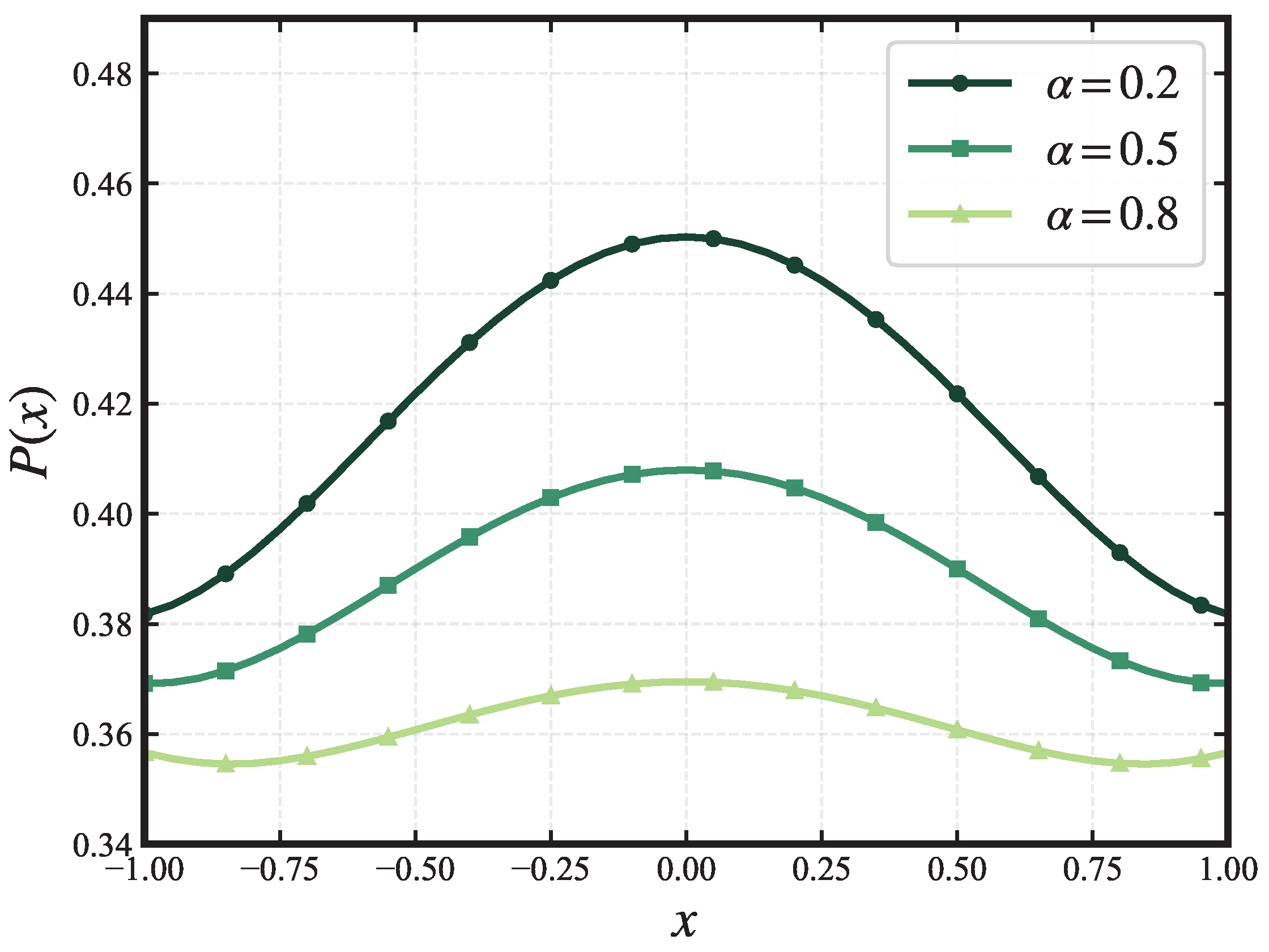
Table 7. The error, convergence order of τ and CPU time for Direct and Fast schemes with fixed h x = h y = 1 / 128 .
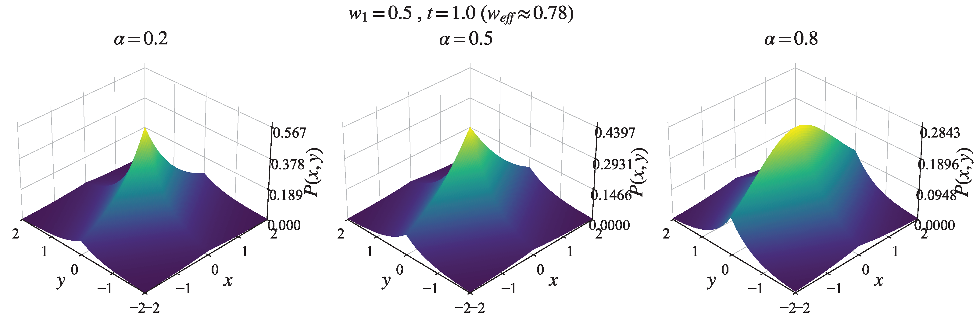
τ DirectFastDirectFast
E r t E r t E r t E r t
α = 0.2 α = 0.4
1/16 7.5148 × 10 5 7.5148 × 10 5 2.3863 × 10 4 2.3863 × 10 4
1/32 3.1078 × 10 5 1.27 3.1078 × 10 5 1.27 8.8817 × 10 5 1.43 8.8817 × 10 5 1.43
1/64 1.7478 × 10 5 0.83 1.7478 × 10 5 0.83 3.7410 × 10 5 1.25 3.7410 × 10 5 1.25
α = 0.6 α = 0.8
1/16 6.3709 × 10 4 6.3709 × 10 4 1.5737 × 10 3 1.5737 × 10 3
1/32 2.5170 × 10 4 1.34 2.5170 × 10 4 1.34 6.9451 × 10 4 1.18 6.9451 × 10 4 1.18
1/64 1.0291 × 10 4 1.29 1.0291 × 10 4 1.29 3.0897 × 10 4 1.17 3.0897 × 10 4 1.17
Table 8. SOE settings reported for the accelerated multi-order solver (Layer C run, M x = M y = 128 , N t = 6400 , T = 0.2 , α = 0.6 ). The table explicitly lists the adopted tolerances, exact short-memory length K exact , selected number of exponentials, and the achieved fitted relative errors for each fractional kernel.
Kernel Order β RoleTolerance ε β K exact L β Rel. Fit Err.
α = 0.6 full-grid history 10 8 859 8.13 × 10 8
α / 2 = 0.3 y-ABC boundary nodes 10 8 8160 2.27 × 10 7
α / 4 = 0.15 backbone endpoints 10 6 860 4.60 × 10 7
Table 9. History-only complexity benchmark for a single fractional order ( β = 0.6 ) with synthetic states ( n dof = 1089 ). This benchmark isolates the temporal history assembly cost and supports the practical complexity advantage of the accelerated scheme over the standard L1 implementation.
N t Direct L1 Time (s)Fast SOE Time (s)Speedup (Direct/Fast)L
2000.0210.0250.84120
4000.0630.0551.15120
8000.2690.1022.64120
16001.1010.2584.27120
32003.3870.4707.21120
64005.8180.8127.17120
Table 10. Small-scale validation of the fully discrete comb-ABC solver, comparing the multi-order accelerated implementation against the standard direct L1 implementation. Configuration: M x = M y = 64 , N t = 800 , T = 0.2 , α = 0.6 , with ( ε α , ε α / 2 , ε α / 4 ) = ( 10 8 , 10 8 , 10 6 ) and K exact = 8 .
MetricValue
max n rel L 2 ( P fast n , P direct n ) 2.757 × 10 11
Final-time rel L 2 ( P fast N t , P direct N t ) 9.797 × 10 12
Final mass (Direct) 0.529988
Final mass (Fast) 0.529988
Relative mass difference at final time 6.468 × 10 12
Disclaimer/Publisher’s Note: The statements, opinions and data contained in all publications are solely those of the individual author(s) and contributor(s) and not of MDPI and/or the editor(s). MDPI and/or the editor(s) disclaim responsibility for any injury to people or property resulting from any ideas, methods, instructions or products referred to in the content.