Maximum Power Extraction from a PMSG-Based Standalone WECS via Neuro-Adaptive Fuzzy Fractional Order Super-Twisting Sliding Mode Control Approach with High Gain Differentiator

Abstract

Maximum Power Point Tracking (MPPT) in permanent-magnet synchronous generator (PMSG)-based wind energy conversion systems (WECS) remains challenging owing to strong nonlinearities, parametric uncertainties, and external disturbances. Conventional sliding mode control (SMC) strategies, while robust, suffer from chattering, dependence on full-state measurements, and degraded performance under model mismatch, limiting their practical deployment. To address these issues, this study proposes a neuroadaptive fuzzy fractional-order super-twisting sliding mode control (Fuzzy-FOSTSMC) integrated with a high-gain observer (HGO) and a radial basis function neural network (RBFNN). The HGO estimates unmeasurable higher-order states (e.g., angular acceleration), enabling output-feedback implementation. In contrast, the RBFNN online approximates unknown nonlinear system dynamics $L_f^{2}h\left(x\right)$ and $L_g{L}_{f}h\left(x\right)$, rendering the controller model-free. Chattering is eliminated by replacing the discontinuous signum function with an adaptive fuzzy boundary layer that dynamically modulates the slope near the sliding surface. Stability is theoretically confirmed by Lyapunov analysis. Extensive MATLAB/Simulink simulations verify that the proposed approach yields a tracking precision of 99.96%, a steady-state speed error of 0.018 rad/s, and a 58.2% reduction in the integral absolute error (IAE) compared to the traditional FOSTSMC. It achieves the optimal power coefficient ($C_p=0.4762$) via TSR control at $7.000\pm 0.002$, under ±30% parametric uncertainties, demonstrating excellent robustness and MPPT effectiveness.

1. Introduction

The worldwide energy system is being fundamentally reshaped to address climate change and the uncertainty of supply from finite fossil fuel sources [1,2]. In this context, it is well known that renewable energy sources, particularly wind, solar, and marine, are the key options. Significantly, global renewable energy consumption increased by 3% in 2020 against a backdrop of decreasing energy demand, and an unprecedented 8% increase in renewable electricity generation in 2021, up to 8300 TWh—its fastest annual growth since the 1970s [3]. Wind and photovoltaic (PV) technologies should account for around two-thirds of new renewable capacity additions, with China accounting for nearly half of global growth, followed by the United States, the European Union, and India. This trend is even more pronounced, given that installed capacity increased rapidly from 175 TWh in 2019–2020 to 275 TWh in 2020–2021, indicative of both technological maturity and falling levelized costs.

Wind energy is captured by WECS, which generally consist of a wind turbine, a gearbox, and an electrical generator connected to the grid via power electronics [4]. Advances in turbine design, such as larger rotor diameters and the introduction of novel power-converter topologies, have led to drastic improvements in the system’s efficiency, scalability, and cost-effectiveness [5,6,7]. However, the time-varying nature of wind speed, along with nonlinearities, parametric uncertainties, and external perturbations inherent in WECS, makes it difficult to operate the system stably and optimally [8]. So, advanced control design is still required to capture maximum energy while maintaining robustness and reliability.

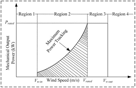
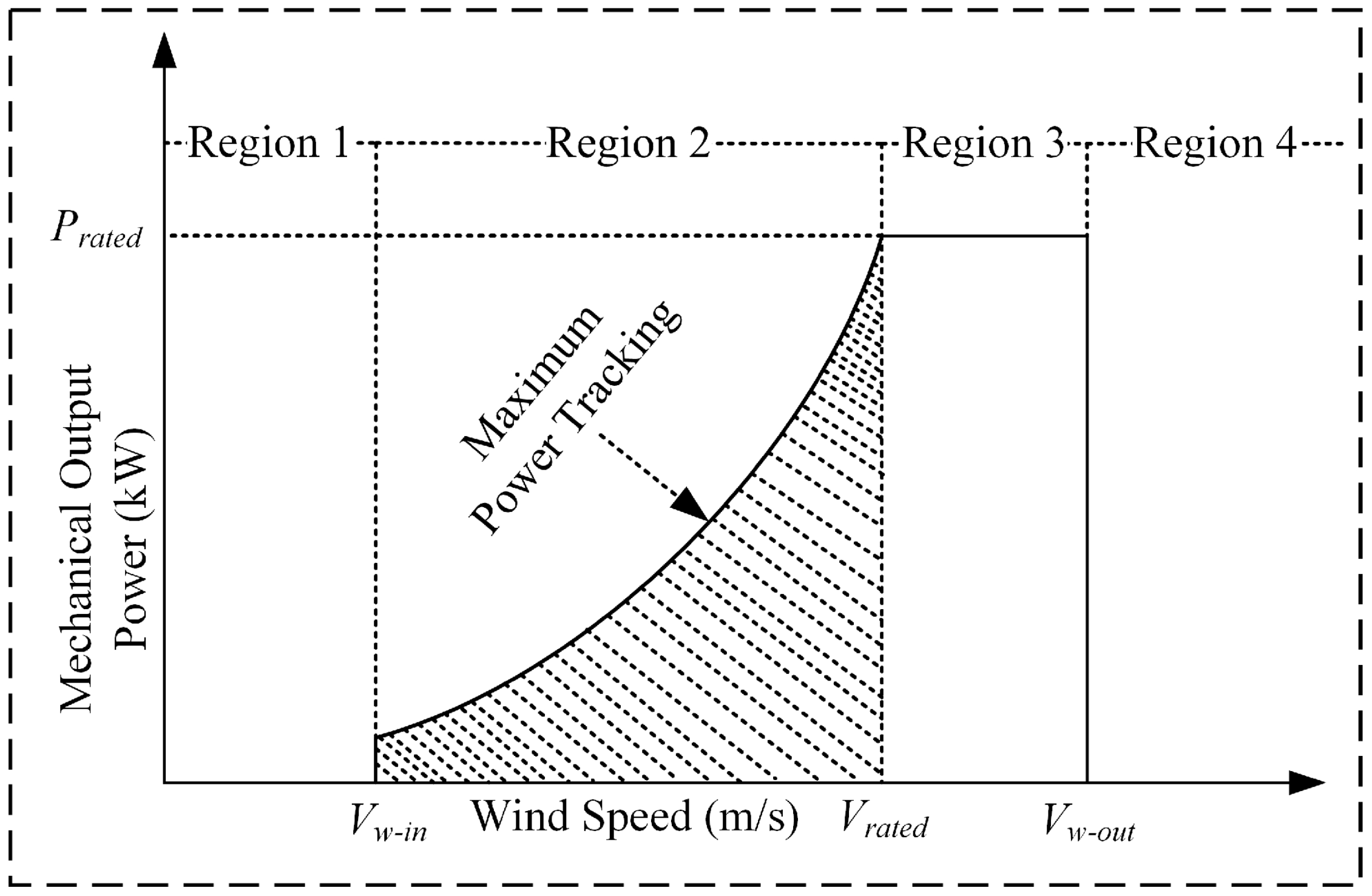
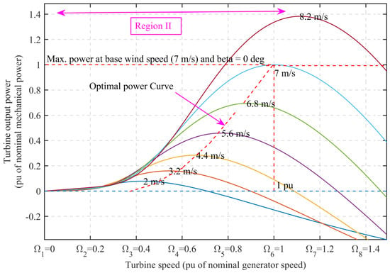
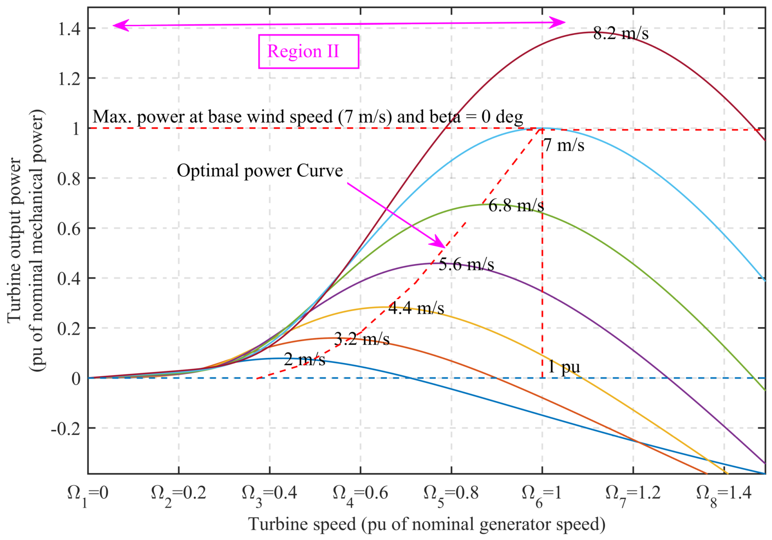
A nominal WECS consists of operation in four different wind-speed regions, as shown in Figure 1 [9,10]. Region 1 ($R_1$) defines the subcut-in wind speeds at which no power is produced. Region 2 ($R_2$) covers the interval between the cut-in speed $V_1$ and the rated speed $V_2$. It is the main area for Maximum Power Point Tracking (MPPT), where variable-speed wind turbines (VSWTs) track rotor speed to maintain the Optimum Tip Speed Ratio (OTSR) and capture the maximum aerodynamic power. Region 3 ($R_3$) is operated at a constant power in the range of [$V_2$, $V_3$], where $V_3$ is the cut-out speed. In Region 4 ($R_4$), the generator is brought to a halt for safety reasons if wind speed is higher than $V_3$. Hence, successful MPPT in Region 2 determines the system’s performance.

Figure 1. The four operating regions of WECS [9,10].

Over the years, a variety of methods have been proposed to perform MPPT, which can be broadly classified into indirect power control (IPC) based on the maximum mechanical power $P_m$ principle and direct power control (DPC) that considers the electrical power $P_e$ explicitly [11]. Standard IPC methods include OTSR control [12], power signal feedback (PSF) [13], and optimal torque algorithms (OTA) [14]. Although PSF and OTA do not require anemometers, they still depend on the parameters of a specific turbine, which limits their use when such parameters are unavailable or vary under uncertain or changing conditions. DPC techniques, including hill-climbing search (HSM) and incremental conductance (INC), are prone to slow convergence and oscillations around the optimum. Conventional linear controllers, such as PI or PID, are more prevalent in industry but often exhibit unsatisfactory performance in the presence of nonlinearities and disturbances due to their fixed gains and limited robustness.

To address these drawbacks, advanced nonlinear control methods have been increasingly studied. Backstepping control [15], model predictive control (MPC) [16], and soft computing methods such as fuzzy logic control (FLC) [17], neural networks [18], and hybrid neuro-fuzzy systems [19], have shown enhanced adaptability. Recently, fault-tolerant control (FTC) schemes, such as neuro-fuzzy qLPV zonotopic observers [20] and MANFIS-based zonotopic fault detectors [21], are being proposed to improve robustness in the presence of sensor or actuator faults. However, they tend to focus more on fault diagnosis than on real-time MPPT operation and may involve complex modeling and/or substantial computational burden.

Sliding mode control (SMC) is a popular strong nonlinear control scheme due to its robustness to matched uncertainties and disturbances [22,23]. However, the traditional first-order SMC exhibits chattering, a high-frequency switching phenomenon caused by the discontinuous signum function, which may excite unmodeled dynamics and shorten hardware life [24]. Although boundary layer smoothing [25] and finite-gain tuning [26] offer partial relief, they compromise tracking accuracy. Higher-order variants, such as the second-order SMC (SOSMC) [27,28] and super-twisting algorithms [29,30], mitigate chattering while preserving robustness but still assume full-state measurements or exact system models. Fractional-order extensions (FOSMC, FOTSMC) [31,32] improve the transient response and disturbance rejection through memory effects; however, they often lack finite-time convergence guarantees under unmatched uncertainties.

Recent composite strategies have integrated SMC with artificial intelligence, such as fuzzy SMC [33], neural-network-enhanced SMC [34], and observer-based designs [35,36], to address model dependency and estimation challenges. Nevertheless, most existing studies treat these components in isolation or use them for gain scheduling rather than for the structural reconfiguration of the control law itself. Crucially, few approaches simultaneously achieve (i) actual chattering elimination without sacrificing robustness, (ii) model-free operation under output feedback, (iii) finite-time convergence in the presence of lumped uncertainties, and (iv) practical feasibility for standalone PMSG-WECS.

To address the aforementioned challenges, the primary objective of this study is to develop a high-performance, chattering-free, and model-free MPPT control strategy for standalone PMSG-based WECS that is robust against parametric uncertainties and external disturbances. As summarized in Table 1, existing approaches either suffer from chattering, rely on full-state measurements, assume known system dynamics, or lack formal guarantees of finite-time convergence under lumped uncertainties. To achieve this, we propose a synergistic neuro-adaptive control framework that integrates a Fuzzy Fractional-Order Super-Twisting Sliding Mode Controller (Fuzzy FOSTSMC) with a Radial Basis Function Neural Network (RBFNN) and an HGO. The RBFNN is employed to online-estimate the unknown nonlinear system dynamics, thereby enabling a model-free control law. Concurrently, the HGO reconstructs the unmeasurable higher-order state derivatives required for control implementation, thereby facilitating a practical output-feedback design. The discontinuous switching component of the controller is replaced with an adaptive fuzzy system to eliminate chattering while preserving robustness, and fractional-order calculus is used to enhance transient response and convergence. The key innovations are:

Table 1. Summary of Related Work and Research Gaps.

Reference	Control Strategy	Key Outcomes	Limitations	Research Gap Addressed
[37,38]	PI/PID Control	Easy implementation, widely used	Fixed gains; poor robustness to nonlinearities/disturbances	Lack of robustness
[15]	Backstepping Control	Good tracking under matched uncertainties	Complex design; requires full-state feedback; sensitive to modeling errors	Full-state dependence and complexity
[16]	Model Predictive Control	Handles constraints; good transient performance	High computational burden; requires accurate model	Computational cost and model reliance
[27,28,29,30]	Super-Twisting SMC	Chattering reduction; robust to matched disturbances	Assumes full-state measurement; still exhibits residual chattering	Output-feedback feasibility & chattering
[31,32]	Fractional-Order SMC	Improved transient response via memory effect	Lacks finite-time convergence; chattering not fully eliminated	Convergence speed and chattering
[33]	Fuzzy-SMC	Reduced chattering via boundary layer smoothing	Rule base often heuristic; limited adaptation to unknown dynamics	Adaptive chattering suppression
[34]	RBFNN-enhanced SMC	Online estimation of uncertainties; improved robustness	Often combined with integer-order SMC; no HGO for state reconstruction	Integration with fractional-order and observer
[35,36]	Observer-based SMC	Enables output-feedback control	Typically uses linear or high-gain observers without neural compensation	Model-free output feedback
Proposed Work	RBFNN + Fuzzy-FOSTSMC + HGO	Chattering-free, model-free, output-feedback, finite-time convergence under lumped uncertainties	—	Simultaneously addresses all above gaps

• A chattering-free reaching law that replaces the discontinuous signum function with an adaptive fuzzy boundary layer whose slope is dynamically modulated by both the sliding surface and its derivative, enabling smooth control action without performance degradation.
• The unknown nonlinear dynamics are compensated using online RBFNN learning of the Lie derivatives $L_f^{2}h\left(x\right)$ and $L_g{L}_{f}h\left(x\right)$, enabling input–output linearization without requiring any knowledge about the exact generator or aerodynamic models.
• An HGO-based output-feedback scheme is devised to accurately reconstruct unmeasurable higher-order states (such as angular acceleration), thereby significantly reducing sensor dependency and improving system deployability in low-cost or harsh-environment applications.
• Finite-time convergence with lumped parametric uncertainty and external disturbance is guaranteed by a positive-definite fractional-power Lyapunov function, which is constructed through a synergistic combination of fractional-order dynamics, super-twisting robustness, and neuro-fuzzy adaptation—an integrated scheme not yet reported for PMSG-based MPPT.

A large number of simulations have been performed in MATLAB/Simulink to verify that the proposed method outperforms the conventional SMC, FOSMC, STSMC, and FOSTSMC in terms of tracking accuracy, chattering reduction, robustness, and convergence rate under actual wind profiles and parametric uncertainties. The outcomes demonstrate that the proposed framework can improve not only tracking accuracy but also the efficiency of the number of expected maxima and minima, and can be extended to practical high-performance control for next-generation wind energy systems.

The rest of the paper is organized as follows. Section 2 introduces the preliminaries of fractional-order calculus. Section 3 presents the modeling of the WECS. The proposed fuzzy fractional-order super-twisting SMC design is detailed in Section 4. Simulation results and discussion are provided in Section 5. Finally, Section 6 concludes the paper and outlines limitations and future research directions.

2. Preliminaries of Fractional-Order Calculus

Fractional calculus extends the concepts of integer-order differentiation and integration to non-integer orders and enables more accurate, flexible modeling of dynamic systems with memory and hereditary effects. Several definitions of fractional derivatives have been proposed, each providing different mathematical formulas for extending classical integer-order calculus [39,40]. In this work, the Riemann–Liouville definition is adopted due to its analytical tractability and suitability for control applications.

Definition 1

([39]). The Riemann–Liouville fractional derivative of order α of a function $f\left(t\right)$, defined over the interval $[t_0,t]$, is given by:

$$D^{\alpha }f\left(t\right)={\displaystyle \frac{1}{\Gamma (m-\alpha )}}{\displaystyle \frac{d^m}{d{t}^m}}{\int }_{t_0}^t{\displaystyle \frac{f\left(\tau \right)}{{(t-\tau )}^{\alpha -m+1}}}d\tau ,$$

(1)

where $m-1\le \alpha <m$, $m\in \mathbb{N}$, and $\Gamma (·)$ denotes the Gamma function.

The corresponding Riemann–Liouville fractional integral of order α is defined as:

$${}_{t_0}I_t^{\alpha }f\left(t\right)={\displaystyle \frac{1}{\Gamma \left(\alpha \right)}}{\int }_{t_0}^t{\displaystyle \frac{f\left(\tau \right)}{{(t-\tau )}^{1-\alpha }}}d\tau .$$

(2)

Lemma 1

([39]). Let $f\left(t\right)$ be a function whose Riemann–Liouville fractional derivative ${}_{a}D_t^{\beta }f\left(t\right)$ exists and is integrable, with $(n-1\le \alpha <n)$. Then, the following property holds:

$$\begin{array}{cc}\hfill {}_{a}D_t^{-\alpha }\left({}_{a}D_t^{\beta }f\left(t\right)\right)& ={}_{a}D_t^{\beta -\alpha }f\left(t\right)-\sum _{j=1}^n{\left[{}_{a}D_t^{\beta -j}f\left(t\right)\right]}_{t=a}·{\displaystyle \frac{{(t-a)}^{\alpha -j}}{\Gamma (1+\alpha -j)}}\hfill \end{array}$$

(3)

Lemma 2

([41,42]). Fractional derivatives and integrals satisfy the following properties:

1.

Semigroup Property:

$${}_{a}D_t^{-\alpha }{}_{a}D_t^{-\beta }f\left(t\right)={}_{a}D_t^{-\alpha -\beta }f\left(t\right)$$

(4)

2.

Composition Rules:

$${\displaystyle \frac{d^n}{d{x}^n}}\left[{}_{a}D_t^{\alpha }f\left(t\right)\right]={}_{a}D_t^{n+\alpha }f\left(t\right)$$

(5)

$$\begin{array}{cc}\hfill {}_{a}D_t^{\alpha }\left[{\displaystyle \frac{d^n}{d{x}^n}}f\left(t\right)\right]& ={}_{a}D_t^{n+\alpha }f\left(t\right)\hfill \\ & -\sum _{j=0}^{n-1}{\displaystyle \frac{f^{\left(j\right)}\left(a\right){(t-a)}^{j-\alpha -n}}{\Gamma (1+j-\alpha -n)}}\hfill \end{array}$$

(6)

where $\alpha >0$, $t\ge a$, $\beta >0$, and $n-1\le \alpha <n$.

Lemma 3

([43]). The fractional integration operator ${}_{a}I_t^{\alpha }$ with $\alpha >0$ is bounded and satisfies the inequality:

$$\parallel I^{\alpha }{y\parallel \le K\parallel y\parallel }_p,0\le K<\infty ,1\le p\le \infty$$

(7)

Lemma 4

([43]). The fractional integration operator ${}_{a}I_t^{\alpha }$ with $\alpha >0$ is bounded and satisfies the inequality:

$$\parallel I^{\alpha }{y\parallel \le K\parallel y\parallel }_p,0\le K<\infty ,1\le p\le \infty$$

(8)

3. Wind Energy Conversion System Modeling

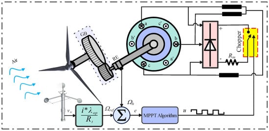
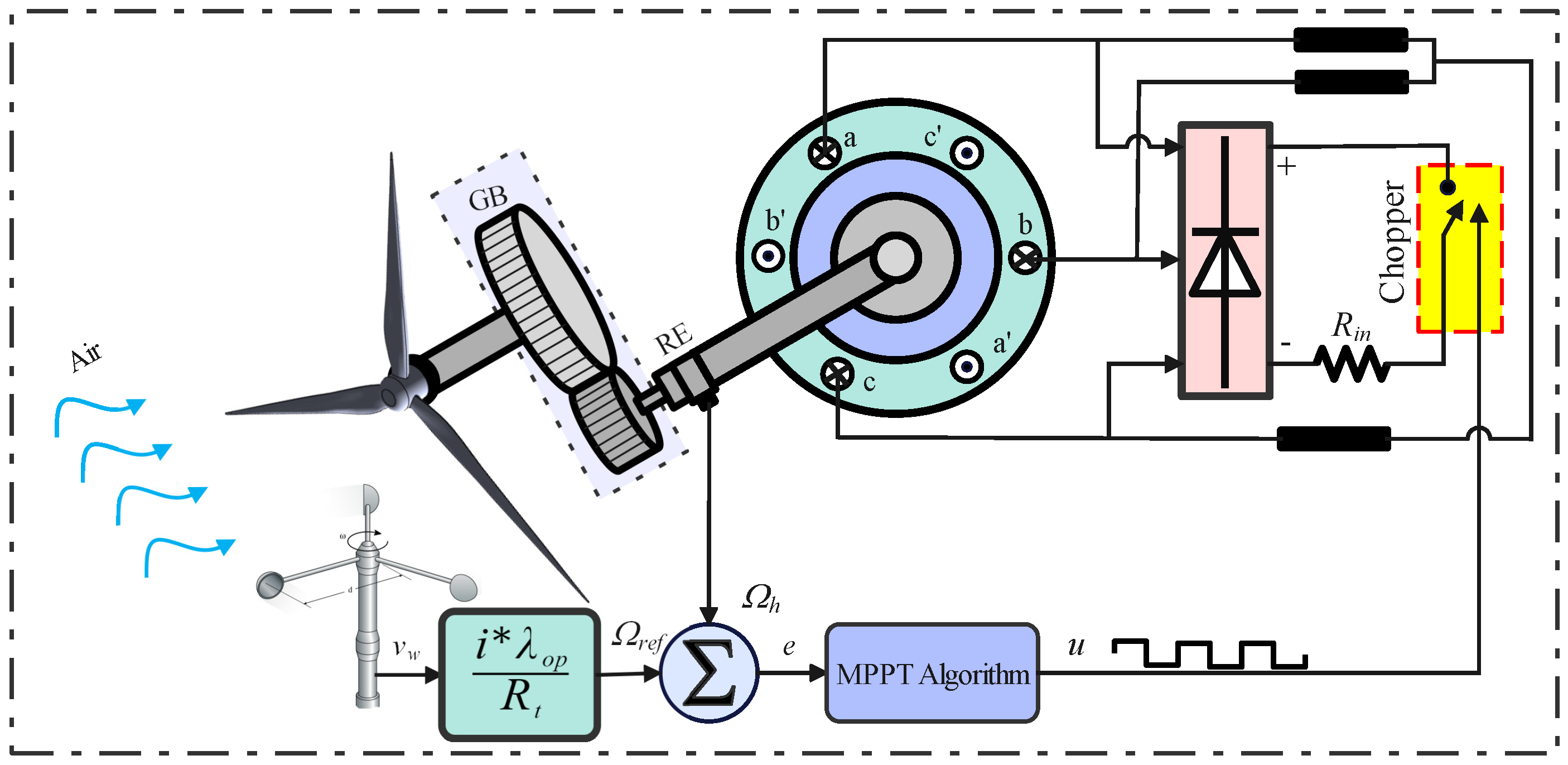
A mathematical description of a wind turbine’s operational behavior is required for performance studies across a range of operating conditions. The complete physical process of WEC is shown in Figure 2 [44]. The mechanical power generation process begins with mechanical power generation from airfoil lift, resulting in a positive torque. Likewise, the mechanical energy is converted into electrical energy by the generator. The rotor-wind interaction (which lies at the core of the entire process) is illustrated in Figure 3. It is astonishing that the average wind speed greatly influences the average generated output power, indicating the importance of including steady aerodynamics when turbulence is not accounted for [45]. A fundamental understanding of wind turbine performance in terms of power and wind load is crucial for assessing wind impacts.

Figure 2. WEC based on PMSG as the central conductor.

Figure 3. Rotational speed of the turbine at different output mechanical powers of the turbine.

The following sections provide brief overviews of the rotor blade and synchronous generator dynamics, which are crucial for control development.

3.1. Wind Turbine Rotor Blades Dynamic Modeling

There are numerous studies focused on the aerodynamic analysis and modeling of VSWTs. Betz was engaged in research on wind turbine aerodynamics during the 1920s and 1930s [46]. In [14], a review on the best design of a wind turbine blade is presented as a multi-blade rotor for wind energy extraction with a maximum power of 59.26% according to the Betz theory in the ideal case. However, in reality, this factor is predicted to drop to 0.5 because of the number of blades and unforeseen variations in external conditions like temperature, wind velocity, and humidity.

The wind turbine power expression can be formulated as:

$$P_{Mech}={\displaystyle \frac{1}{2}}{\rho }_{air}{A}_b{V}_{wind}^3$$

(9)

where $V_{wind}$ the wind velocity (in m/s), $A_b$ the area of the blade swept, ${\rho }_{air}$ the density of air, and $P_{Mech}$ is the mechanical output power of the turbine. The wind turbine rotor power conversion ratio (also known as the power coefficient) $C_p(\lambda ,\beta )$ is the amount of power that can be extracted over the amount of power available. It is modeled in [41] as follows:

$$P_{Mech}={\displaystyle \frac{1}{2}}\pi {\rho }_{air}{R}_{tb}^2{V}_{wind}^3{C}_p(\lambda ,\beta )$$

(10)

where $\lambda$ is the tip-speed ratio (TSR), $\beta$ is the blade pitch angle, and $R_{tb}$ is the radius of the blade in m. The TSR is the angular speed of the turbine relative to the linear speed of wind flow in the free stream, given by,

$$\lambda ={\displaystyle \frac{R_{tb}{\Omega }_h}{V_{wind}}}$$

(11)

where ${\Omega }_h$, $R_{tb}$, and $V_{wind}$ refer to the angular velocity of the rotor, the radius of the rotor, and the wind velocity, respectively, and the power coefficient $C_P$ depends on the variables $\lambda$ and $\beta$. To achieve the maximum power extraction from wind, the tip speed ratio has to be run at its optimum value, which is equal to ${\lambda }_{opt}=7$. The speed of the rotor shaft at this optimal TSR is then used as the reference speed ${\omega }_{ref}$, which is calculated as:

$${\Omega }_{ref}={\displaystyle \frac{{\lambda }_{opt}{V}_{wind}}{R_{tb}}}$$

(12)

For a variable-speed wind turbine, the power coefficient $C_p$ can be approximated as a polynomial function of the tip-speed ratio $\lambda$ by assuming a fixed pitch angle ($\beta =0$) as follows [25]:

$$C_p\left(\lambda \right)={\alpha }_1\lambda +{\alpha }_2{\lambda }^2+{\alpha }_3{\lambda }^3+{\alpha }_4{\lambda }^4+{\alpha }_5{\lambda }^5+{\alpha }_6{\lambda }^6+{\alpha }_7{\lambda }^7$$

(13)

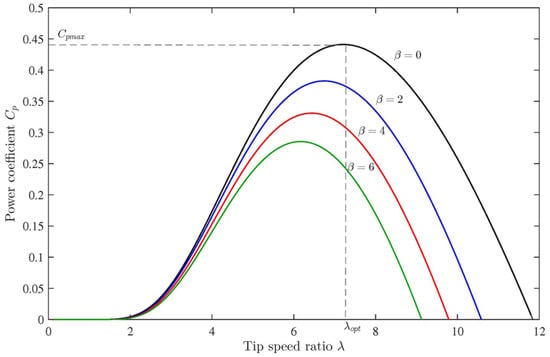
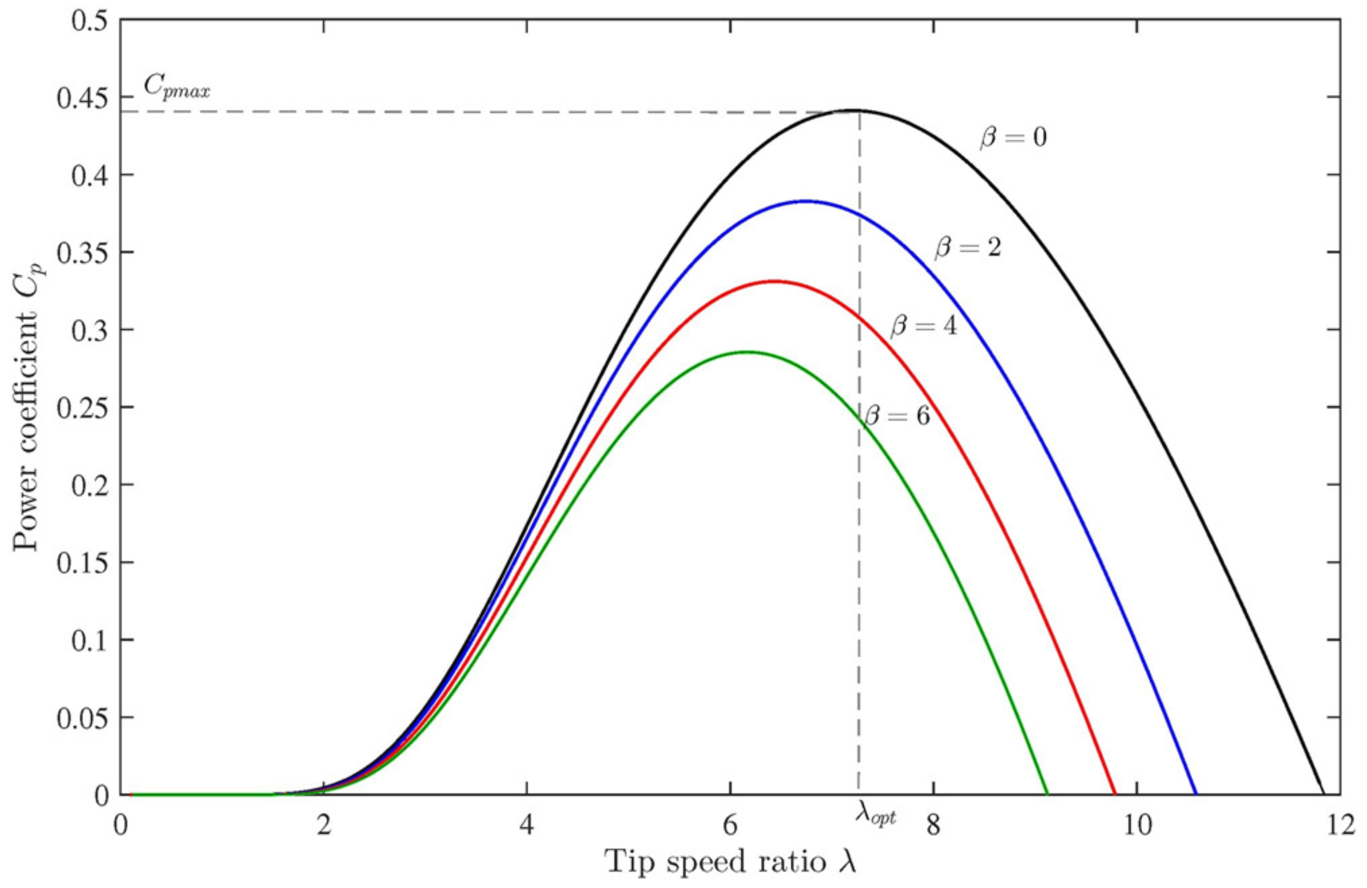
where ${\alpha }_1=6.1\times {10}^{-3}$, ${\alpha }_2=-1.3\times {10}^{-3}$, ${\alpha }_3=8.1\times {10}^{-3}$, ${\alpha }_4=-9.74\times {10}^{-4}$, ${\alpha }_5=6.54\times {10}^{-5}$, ${\alpha }_6=1.30\times {10}^{-6}$, and ${\alpha }_7=-4.54\times {10}^{-7}$. The theoretical upper bound of the power coefficient, known as the Betz limit, is approximately 0.47 [26]. The variation of the power coefficient $C_p$ with respect to the tip-speed ratio for different pitch angles is shown in Figure 4. For each pitch angle $\beta$, the $C_p-\lambda$ characteristic exhibits a unique maximum value $C_{p,max}$ at an optimal tip-speed ratio ${\lambda }_{opt}$. Therefore, by regulating the rotor speed to maintain operation at ${\lambda }_{opt}$, the variable-speed wind turbine can continuously track the maximum power point and extract the maximum available wind energy.

Figure 4. Power coefficient versus tip speed ratio under different pitch angles.

The mechanical torque of the turbine shaft is the output mechanical power divided by the shaft’s angular velocity.

$$\mathrm{Turbine}\mathrm{mechanical}\mathrm{torque}=\mathrm{Output}\mathrm{Mechanical}\mathrm{Power}/\mathrm{Rotor}\mathrm{Speed}$$

(14)

This equation can be written as follows:

$$P_{Mech}={\Gamma }_{Mech}{\Omega }_h$$

(15)

Substituting Equations (10) and (11) into Equation (15), one may get the following expression

$${\Gamma }_{Mech}={\displaystyle \frac{1}{2}}\pi {\rho }_{air}{R}_{tb}^3{V}_{wind}^2{C}_{\Gamma }\left(\lambda \right)$$

(16)

where the turbine torque coefficient $C_{\Gamma }\left(\lambda \right)$ is the power coefficient $C_p\left(\lambda \right)$ divided by the tip speed ratio $\lambda$, ${\rho }_{air}$ is the density of the air, $R_{tb}$ is the radius of the turbine, and $V_{wind}$ is the velocity of the wind. Using Equations (11) and (13) in Equation (16) and neglecting the higher-order $\lambda$ terms, the aerodynamic power can be approximated as:

$${\Gamma }_{Mech}=d_1{V}_{wind}^2+d_2{V}_{wind}{\Omega }_h+d_3{\Omega }_h^2$$

(17)

where $d_1={\displaystyle \frac{1}{2}}\pi {\rho }_{air}{R}_{tb}^3{\alpha }_1$, $d_2={\displaystyle \frac{1}{2}}\pi {\rho }_{air}{R}_{tb}^4{\alpha }_2$, and $d_3={\displaystyle \frac{1}{2}}\pi {\rho }_{air}{R}_{tb}^5{\alpha }_3$.

All the required parameters of the wind turbine employed in this study are given in Table 2.

Table 2. Parameters of the wind turbine.

Parameters	Symbols	Value	Units
Blade Radius	$R_{tb}$	2.5	m
Maximum Power Coefficient	$C_{p_{max}}$	0.47
Gears Ratio/Transmission Ratio	i	7
Air density	$\rho$	1.25	kg/m3
High Speed Shaft Inertia	$j_h$	0.0552	kg
Optimal Tip Speed Ratio	${\lambda }_{opt}$	7

3.2. Electrical Subsystem Modelling

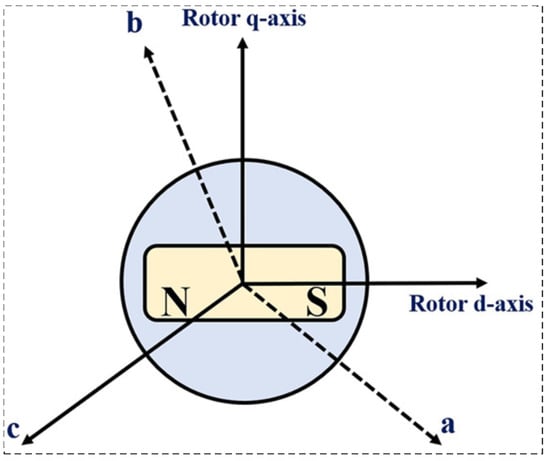
Using Park’s transformation, the three-phase dynamics of the PMSG are mapped onto a single-phase equivalent system. The PMSG comprises three stator windings (a, b, and c), where the d-axis is oriented along the rotor flux and the q-axis in the perpendicular direction, as illustrated in Figure 5.

Figure 5. Three-phase PMSG with the single pole covered by a magnet.

The current along the d-axis is obtained by combining the contributions from the stator windings projected onto the direct axis:

$$i_d=k_d[i_a\cos \left(\theta \right)+i_b\cos (\theta -120)+i_c\cos (\theta +120)]$$

(18)

In the same way, the q-axis current is given as follows:

$$i_q=k_q[i_a\sin \left(\theta \right)+i_b\sin (\theta -120)+i_c\sin (\theta +120)]$$

(19)

where $k_d,k_q$ are positive scalars, and $\theta$ is the angle between the phase a axis and the rotor direct axis. For dimensionality, the zero-sequence current is also established by making use of Kirchhoff’s current law.

$$i_0=k_0[i_a+i_b+i_c]$$

(20)

where $k_d=k_q={\displaystyle \frac{2}{3}}$ and $k_0={\displaystyle \frac{1}{3}}$. Equations (18)–(20) can be written in a concise matrix form:

$$\left[\begin{array}{c}{i}_d\\ i_q\\ i_0\end{array}\right]={\displaystyle \frac{2}{3}}\left[\begin{array}{ccc}\cos \left(\theta \right)& \cos (\theta -120)& \cos (\theta -120)\\ \sin \left(\theta \right)& \sin (\theta -120)& \sin (\theta +120)\\ {\displaystyle \frac{1}{2}}& {\displaystyle \frac{1}{2}}& {\displaystyle \frac{1}{2}}\end{array}\right]\left[\begin{array}{c}{i}_a\\ i_b\\ i_c\end{array}\right]$$

(21)

Park’s transformation matrix P can be used to transform currents, voltages, and fluxes. The resulting currents, voltages, and fluxes in the transformed $dq0$ model are given by

$$\begin{array}{cc}\hfill i_{dq0}& =P{i}_{abc}\hfill \\ \hfill v_{dq0}& =P{v}_{abc}\hfill \\ \hfill {\Psi }_{dq0}& =P{\Psi }_{abc}\hfill \end{array}$$

(22)

and their inverse transformations are

$$\begin{array}{cc}\hfill i_{abc}& =P^{-1}{i}_{dq0}\hfill \\ \hfill v_{abc}& =P^{-1}{v}_{dq0}\hfill \\ \hfill {\Psi }_{abc}& =P^{-1}{\psi }_{dq0}\hfill \end{array}$$

(23)

The Kirchhoff’s voltage-law equations in the a, b, and c stator windings are formulated according to source or generator conventions. Applying Kirchhoff’s voltage law, it follows that:

$$v_k=R_k{i}_k+{\displaystyle \frac{d\Psi }{dt}}$$

(24)

where $k=a, b, \mathrm{and} c$. Adding these equations results in

$$P^{-1}{v}_{dq0}=R_a{P}^{-1}{i}_{dq0}+{\displaystyle \frac{d\left(P^{-1}{\Psi }_{dq0}\right)}{dt}}$$

(25)

Multiplying both sides from the left by P gives:

$$v_{dq0}=R_a{i}_{dq0}+P{\displaystyle \frac{d\left(P^{-1}{\Psi }_{dq0}\right)}{dt}}$$

(26)

After making simplifications, the q-axis and d-axis voltage equations are rewritten as follows:

$$\begin{array}{cc}\hfill v_d& =R_a{i}_d+{\displaystyle \frac{d{\Psi }_d}{dt}}-{\Psi }_q\hfill \\ \hfill v_q& =R_a{i}_q+{\displaystyle \frac{d{\Psi }_q}{dt}}+{\Psi }_d\hfill \end{array}$$

(27)

The direct and quadrature axis fluxes, ${\Psi }_d$ and ${\Psi }_q$, are expressed as:

$$\begin{array}{cc}\hfill {\Psi }_d& =L_d{i}_d+{\varphi }_m\hfill \\ \hfill {\Psi }_q& =L_q{i}_q\hfill \end{array}$$

(28)

After simplification, the final $dq$-model equations for the PMSG are

$$\begin{array}{cc}\hfill v_d& =R_a{i}_d+L_d{\displaystyle \frac{d}{dt}}{i}_d-L_q{i}_q\hfill \\ \hfill v_q& =R_a{i}_q+L_q{\displaystyle \frac{d}{dt}}{i}_q+(L_d{i}_d+{\varphi }_m)\hfill \end{array}$$

(29)

where $v_q$ and $v_d$ are the $dq$-axis voltages, $L_q=L_d=L$ for a non-salient PMSG, ${\Phi }_m$ is the permanent magnet flux, and $R_a$ is the stator resistance. The electromagnetic torque is defined as:

$$\begin{array}{cc}\hfill T_{em}& =p\left[{\varphi }_m{i}_q+(L_d-L_q)i_d{i}_q\right]\hfill \\ \hfill & =p{\varphi }_m{i}_q\hfill \end{array}$$

(30)

3.3. State-Space Representation of System Dynamics

The system comprises three state variables: $i_d$, $i_q$, and ${\Omega }_h$. For the purpose of controller derivation, the PMSG equations are expressed in the form of a nonlinear dynamical system:

$$\begin{array}{cc}\hfill {\dot{x}}_1& ={\displaystyle \frac{-R_s{x}_1+p\left(L_q{L}_{ch}\right)x_2{x}_3-R_{ini}{x}_1}{(L_d+L_{ch})}}\hfill \\ \hfill {\dot{x}}_2& ={\displaystyle \frac{-R_s{x}_2-p(L_d+L_{ch})x_1{x}_3-R_{ini}{x}_2}{(L_q+L_{ch})}}+p{\varphi }_m{x}_3\hfill \\ \hfill {\dot{x}}_3& ={\displaystyle \frac{\frac{d_1{v}_w^2}{i}+\frac{d_2{v}_w{x}_3}{i^3}+\frac{d_3{x}_3^2}{i^3}-p{\varphi }_m{x}_2}{J_h}}\hfill \end{array}$$

(31)

where ${\varphi }_m$ is the flux; $d_1$, $d_2$, and $d_3$ are the constants; p is the number of pole pair; $R_{ini}$ and $R_s$ are the chopper equivalence and stator resistances, respectively; $v_w$ is the wind velocity; $L_d$, $L_q$, and $L_{ch}$ denote the direct-axis, quadrature-axis, and chopper inductances, respectively; $x_1$, $x_2$, and $x_3$ are the states $i_d$, $i_q$, and ${\omega }_h$, respectively; and $J_h$ stand for the moment of inertia.

The system (25) state equations can also be expressed as

$$\begin{array}{cc}\hfill \left[\begin{array}{c}{\dot{x}}_1\\ {\dot{x}}_2\\ {\dot{x}}_2\end{array}\right]& =\left[\begin{array}{c}{\displaystyle \frac{-R_s{x}_1+p\left(L_q{L}_{ch}\right)x_2{x}_3}{(L_d+L_{ch})}}\\ {\displaystyle \frac{-R_s{x}_2-p(L_d+L_{ch})x_1{x}_3}{(L_q+L_{ch})}}+p{\varphi }_m{x}_3\\ {\displaystyle \frac{\frac{d_1{v}_w^2}{i}+\frac{d_2{v}_w{x}_3}{i^3}+\frac{d_3{x}_3^2}{i^3}-p{\varphi }_m{x}_2}{J_h}}\end{array}\right]+\left[\begin{array}{c}{\displaystyle \frac{-R_{ini}{x}_1}{(L_d+L_{ch})}}\\ {\displaystyle \frac{-R_{ini}{x}_2}{(L_q+L_{ch})}}\\ 0\end{array}\right]u\hfill \\ \hfill y& =h\left(x\right)=\left[\begin{array}{ccc}0& 0& 1\end{array}\right]\left[\begin{array}{c}{x}_1\\ x_2\\ x_3\end{array}\right]\hfill \end{array}$$

(32)

The PMSG employed in the system (26) has the parameters given in Table 3.

Table 3. Parameters of the PMSG.

Parameters	Symbols	Value	Units
Stator Resistance	$R_s$	3.3	Ohm
Direct-axis Inductance	$L_d$	$41.56\times {10}^{-3}$	H
Quadrature-axis Inductance	$L_q$	$41.56\times {10}^{-3}$	H
Chopper Inductance	$L_{ch}$	0.08	Henry
Pole Pair Number	p	3	-
Flux	${\varphi }_m$	0.4382	Wb
Chopper Equivalence Resistance	$R_{ini}$	80	ohm

3.4. System Relative Degree

The relative degree of the system is computed prior to the input–output transformation to satisfy the conditions for controller synthesis. For the PMSG-WECS, this relative degree, r, is determined as:

$$L_g{L}_f^{r-1}h\left(x\right)\ne 0\mathrm{For}\mathrm{values}\mathrm{of}\mathrm{r}=1,2,3, \dots ,$$

(33)

where $L_g$ and $L_f$ are the Lie derivative operator with respect to vector fields $g\left(x\right)$ and $f\left(x\right)$, respectively. The Lie derivative of a scalar function $h\left(x\right)$ along the flow of a vector field $f\left(x\right)$ is given by:

$$L_{f}h\left(x\right)={\displaystyle \frac{\partial h\left(x\right)}{\partial x}}f\left(x\right)$$

In the same way, we have the Lie derivative of $h\left(x\right)$ with respect to $g\left(x\right)$ is

$$L_{g}h\left(x\right)={\displaystyle \frac{\partial h\left(x\right)}{\partial x}}g\left(x\right)$$

First order Lie derivative $L_{f}h$ is defined for any $k\ge 2$ recursively as follows:

$$L_f^{k}h\left(x\right)=L_f(L_f^{k-1}h(x))\ge 2$$

These derivatives play a key role in input–output linearization and in characterizing the relative degree of nonlinear systems. Based on the nonlinear system form, the nonlinear functions $f\left(x\right)$ and $g\left(x\right)$ of the system (32) are as follows

$$\begin{array}{cc}\hfill f\left(x\right)& =\left[\begin{array}{c}{f}_1\left(x\right)\\ f_2\left(x\right)\\ f_3\left(x\right)\end{array}\right]=\left[\begin{array}{c}{\displaystyle \frac{-R_s{x}_1+p\left(L_q{L}_{ch}\right)x_2{x}_3}{(L_d+L_{ch})}}\\ {\displaystyle \frac{-R_s{x}_2-p(L_d+L_{ch})x_1{x}_3}{(L_q+L_{ch})}}+p{\varphi }_m{x}_3\\ {\displaystyle \frac{1}{J_h}}\left({\displaystyle \frac{d_1{v}_w^2}{i}}+{\displaystyle \frac{d_2{v}_w{x}_3}{i^3}}+{\displaystyle \frac{d_3{x}_3^2}{i^3}}-p{\varphi }_m{x}_2\right)\end{array}\right]\hfill \\ \hfill g\left(x\right)& =\left[\begin{array}{c}{g}_1\left(x\right)\\ g_2\left(x\right)\\ g_3\left(x\right)\end{array}\right]=\left[\begin{array}{c}{\displaystyle \frac{-R_{ini}{x}_1}{(L_d+L_{ch})}}\\ {\displaystyle \frac{-R_{ini}{x}_2}{(L_q+L_{ch})}}\\ 0\end{array}\right]\hfill \\ \hfill u& =R_{ini}\hfill \end{array}$$

(34)

To find the relative degree, let $r=1$. The Lie derivative of $h\left(x\right)$ along g is computed as

$$L_g{L}_f^{r-1}h\left(x\right)=L_{g}h\left(x\right)={\displaystyle \frac{\partial h\left(x\right)}{\partial x}}.g\left(x\right)=\left[\begin{array}{ccc}0& 0& 1\end{array}\right]\left[\begin{array}{c}{x}_1\\ x_2\\ x_3\end{array}\right]=0$$

(35)

Since the relative degree ($r=1$) is not compatible with this condition, we instead consider the case ($r=2$).

$$L_g{L}_{f}h\left(x\right)={\displaystyle \frac{p{\varphi }_m{x}_2}{J_h(L_q+L_{ch})}}\ne 0$$

(36)

Thus, the proposed PMSG-based WECS exhibits a relative degree of 2.

3.5. Key Modeling Assumptions

For controller design and analysis, the following assumptions are considered for the PMSG-based WECS model:

• Small-scale turbulence effects are not explicitly modeled. This simplification allows focusing on controller performance under variable wind speeds, while the proposed Fuzzy-FOSTSMC can still accommodate moderate wind fluctuations observed in practice.
• All system parameters, including rotor inductances, stator resistance, and permanent magnet flux, are assumed to lie within known physical limits. These bounds are incorporated into the controller design to ensure robustness against parameter uncertainties.
• Sensor measurements are assumed to be bounded and of typical industrial accuracy. The high-gain observer and RBFNN design account for bounded disturbances, ensuring robust control performance in the presence of measurement noise.

These assumptions simplify the modeling process without compromising the demonstration of the proposed controller’s effectiveness.

In the next subsection, the system is reformulated into an appropriate input–output representation for control purposes.

3.6. Input–Output Form Transformation

The general nonlinear system with input $u\in {\mathbb{R}}^m$, output $y=h\left(x\right)\in {\mathbb{R}}^l$, and state $x\in {\mathbb{R}}^n$ is given by

$$\begin{array}{c}\hfill \dot{x}=f\left(x\right)+g\left(x\right)u,y=h\left(x\right)\end{array}$$

(37)

where $f\left(x\right)\in {\mathbb{R}}^n$ denotes the nonlinear smooth state vector field, and $g\left(x\right)\in {\mathbb{R}}^{n\times m}$ is a matrix composed of smooth functions. In the context of the PMSG-WECS system, the state vector x is given by:

$$x=\left[\begin{array}{c}{x}_1\\ x_2\\ x_3\end{array}\right]=\left[\begin{array}{c}{i}_d\\ i_q\\ {\omega }_h\end{array}\right]$$

(38)

We can write the system dynamics as

$$\begin{array}{cc}\hfill {\dot{x}}_1& =-k_1{x}_1-k_2{x}_2{x}_3-k_{3}u{x}_1\hfill \\ \hfill {\dot{x}}_2& =-l_1{x}_2-l_2{x}_1{x}_3+l_3{x}_3-l_{4}u{x}_2\hfill \\ \hfill {\dot{x}}_3& =-m_1-m_2{x}_3-m_3{x}_3^2-m_4{x}_2\hfill \end{array}$$

(39)

In which, the functions $f\left(x\right)$ and $g\left(x\right)$ are defined as follows:

$$\begin{array}{cc}\hfill f\left(x\right)& =\left[\begin{array}{c}{f}_1\left(x\right)\\ f_2\left(x\right)\\ f_3\left(x\right)\end{array}\right]=\left[\begin{array}{c}-k_1{x}_1-k_2{x}_2{x}_3\\ -l_1{x}_2-l_2{x}_1{x}_3+l_3{x}_3\\ -m_1-m_2{x}_3-m_3{x}_3^2-m_4{x}_2\end{array}\right]\hfill \\ \hfill g\left(x\right)& =\left[\begin{array}{c}{g}_1\left(x\right)\\ g_2\left(x\right)\\ g_3\left(x\right)\end{array}\right]=\left[\begin{array}{c}-k_3{x}_1\\ l_{4}u{x}_2\\ 0\end{array}\right]\hfill \end{array}$$

(40)

By plugging Equations (34) into (31), we have the next Equation.

$$\begin{array}{cc}\hfill \left[\begin{array}{c}{\dot{x}}_1\\ {\dot{x}}_2\\ {\dot{x}}_3\end{array}\right]& =\left[\begin{array}{c}-k_1{x}_1-k_2{x}_2{x}_3\\ -l_1{x}_2-l_2{x}_1{x}_3+l_3{x}_3\\ -m_1-m_2{x}_3-m_3{x}_3^2-m_4{x}_2\end{array}\right]+\left[\begin{array}{c}-k_3{x}_1\\ l_{4}u{x}_2\\ 0\end{array}\right]u\hfill \\ \hfill y& =h\left(x\right)=\left[\begin{array}{ccc}0& 0& 1\end{array}\right]\left[\begin{array}{c}{x}_1\\ x_2\\ x_3\end{array}\right]\hfill \end{array}$$

(41)

In Equation (35), the control input u is defined as

$$u=R_{ini}$$

(42)

The dummy variables z in the inverse coordinate transformation are given by:

$$z=\left[z_1,L_{f}h\left(x\right),L_f^{2}h\left(x\right),\dots ,L_f^{r-1}h\left(x\right)\right]$$

(43)

The terms $z_1$, $z_2$, and $z_3$ are expressed as follows

$$\begin{array}{cc}\hfill z_1& =x_3\hfill \\ \hfill z_2& =L_{f}h\left(x\right)=\left[\begin{array}{ccc}0& 0& 1\end{array}\right]\left[\begin{array}{c}-k_1{x}_1-k_2{x}_2{x}_3\\ -l_1{x}_2-l_2{x}_1{x}_3+l_3{x}_3\\ -m_1-m_2{x}_3-m_3{x}_3^2-m_4{x}_2\end{array}\right]\hfill \\ \hfill z_3& =L_f^{2}h\left(x\right)={\displaystyle \frac{x_1}{x_2}}\hfill \end{array}$$

(44)

The inverse coordinate transformation is given by

$$\begin{array}{cc}\hfill x_1& =z_3{\displaystyle \frac{(m_1-z_2-m_2{z}_1-m_3{z}_1^2)}{m_4}}\hfill \\ \hfill x_2& ={\displaystyle \frac{(m_1-z_2-m_2{z}_1-m_3{z}_1^2)}{m_4}}\hfill \\ \hfill x_3& =z_1\hfill \end{array}$$

(45)

Next, system equations are derived in the z-domain as

$$\begin{array}{cc}\hfill {\dot{z}}_1& ={\dot{x}}_3=z_2\hfill \\ \hfill {\dot{z}}_2& =L_f^{2}h\left(x\right)+L_g{L}_{f}h\left(x\right)u\hfill \end{array}$$

(46)

The Lie derivatives are given by

$$\begin{array}{cc}\hfill L_f^{2}h\left(x\right)& =m_4{f}_2-(m_2+2m_3{x}_3)f_3\hfill \\ \hfill L_f{L}_{g}h\left(x\right)& =l_4{m}_4{x}_2\hfill \end{array}$$

(47)

Then, the equivalent linearized system is

$$\begin{array}{cc}\hfill \left[\begin{array}{c}{\dot{z}}_1\\ {\dot{z}}_2\end{array}\right]& =\left[\begin{array}{cc}0& 1\\ 0& 0\end{array}\right]\left[\begin{array}{c}{z}_1\\ z_2\end{array}\right]+\left[\begin{array}{c}0\\ 1\end{array}\right]u\hfill \\ \hfill y& =\left[\begin{array}{cc}1& 0\end{array}\right]\left[\begin{array}{c}{z}_1\\ z_2\end{array}\right]\hfill \end{array}$$

(48)

The proposed sliding mode controller will construct the control input u.

In the next subsection, the stability properties of the system’s third internal dynamic state are analyzed.

3.7. Zero-Dynamic Stability Investigation of the System

After completing all calculations and performing the transformation into the z-coordinate system, the third internal dynamic state of the system is obtained as follows:

$$\begin{array}{cc}\hfill {\dot{z}}_3& ={\displaystyle \frac{m_4}{m_1}}\left(-{\displaystyle \frac{k_1{z}_3{m}_1}{m_4}}-{\displaystyle \frac{k_2{z}_1{m}_1}{m_4}}-{\displaystyle \frac{k_3{z}_3{m}_{1}u}{m_4}}\right)-{\displaystyle \frac{z_3{m}_1}{m_4}}\left(\begin{array}{c}{m}_4^2\\ m_1^2\end{array}\right)\hfill \\ \hfill & \left(-{\displaystyle \frac{l_1{m}_1}{m_4}}-{\displaystyle \frac{l_2{m}_1{z}_3{z}_1}{m_4}}+l_3{z}_1-{\displaystyle \frac{l_4{m}_{1}u}{m_4}}\right)\hfill \end{array}$$

(49)

To analyze the stability of the zero dynamics, impose $z_1=z_2=u=0$. Substituting these conditions into Equation (43) yields the following expression:

$${\dot{z}}_3=-z_3(k_1-l_1)$$

(50)

where the constants $k_1$ and $l_1$ are defined as $k_1={\displaystyle \frac{R_s+R_{ini}}{L_d+L_{ch}}}$ and $l_1={\displaystyle \frac{R_s+R_{ini}}{L_q+L_{ch}}}$. Given the design constant $k_1>l_1$, the following equation can be derived:

$${\dot{z}}_3=-k_1{z}_3$$

(51)

where the zero-dynamic state is stable for all $k_1>l_1$.

Before proceeding to the control law design for duty-cycle regulation and maximum power extraction, the following standard assumptions are introduced:

Assumption 1.

The RBFNN approximation errors are uniformly bounded over a compact set

$$|e_{L_f^{2}h}\left(x\right)|\le {\Xi }_1,|e_{L_g{L}_{f}h}\left(x\right)|\le {\Xi }_2,\Xi =max({\Xi }_1,{\Xi }_2)>0.$$

Assumption 2.

The ideal weight vectors $W_{L_f^{2}h\left(x\right)}$ and $W_{L_g{L}_{f}h}$ are bounded, i.e., $\parallel W\parallel \le W_{max}<\infty$.

Assumption 3.

The reference trajectory $z_{1,ref}\left(t\right)$ and its first two time derivatives are smooth and are bounded.

Assumption 4.

The estimated Lie derivative ${\widehat{L}}_g{L}_{f}h\left(x\right)\ge \underline{\mathcal{l}}>0$ for all x in the operating domain, ensuring the well-posedness of the control law.

4. Design of Fuzzy Fractional Order Super-Twisting Sliding Mode Control

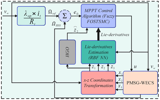
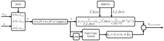
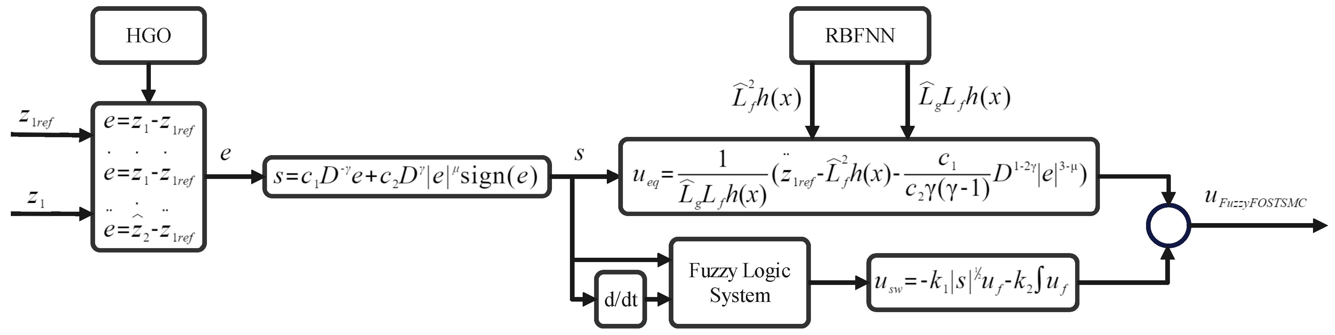
This study presents a novel MPPT strategy for wind turbines that addresses external disturbances and parametric uncertainties through an RBFNN–based fuzzy fractional-order super-twisting sliding mode control (Fuzzy-FOSTSMC). Fractional calculus is embedded in the sliding surface to improve robustness and dynamic performance under uncertainties. The fractional-order structure provides additional tuning flexibility, leading to enhanced tracking accuracy and stronger disturbance rejection [32,34,47]. The proposed scheme also suppresses undesirable fluctuations that can degrade rotor dynamics. The overall control architecture is shown in Figure 6. To reduce sensitivity to unknown disturbances, an RBFNN and a high-gain differentiator are integrated within the Fuzzy-FOSTSMC framework to ensure accurate tracking of the wind speed reference and optimal power extraction. The detailed controller formulation is provided in Equations (48) and (50), assuming stable internal (zero) dynamics.

Figure 6. Schematic representation of the overall control system.

In the next subsection, the control design integrating the RBF neural network with a HGO is detailed.

4.1. Radial Basis Function Neural Network Architecture

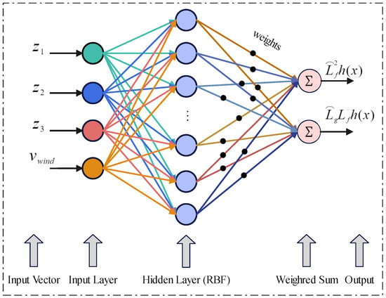
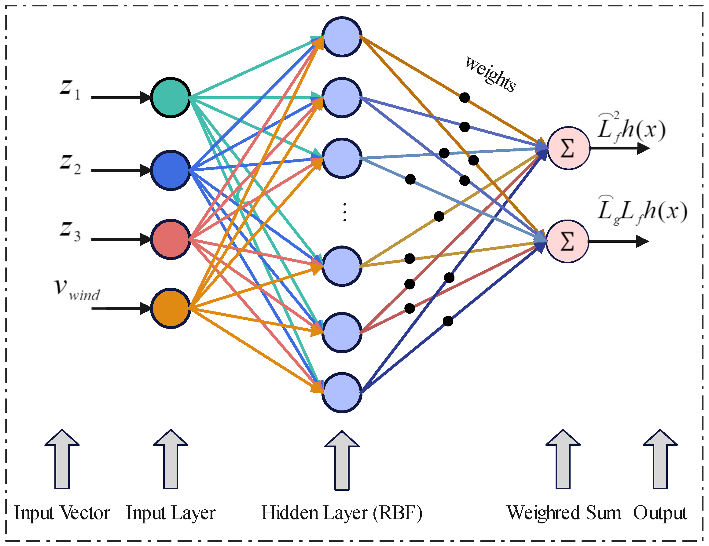
The feedback control input relies on estimates of the nonlinear drift functions. Thus, the input channel $L_g{L}_{f}h\left(x\right)$ and the nonlinear drift term $L_f^{2}h\left(x\right)$ are represented using a radial basis function neural network, where the choice of approximation functions depends on the characteristics of the system. This approach suppresses chattering and provides robust performance, with network weights updated through Lyapunov-based adaptive laws to continuously track and maintain the estimated functions. The network adapts to new system contexts by learning from the input vector $x=[z_1,z_2,z_3,v_{\mathrm{wind}}]$ and the target functions ${\widehat{L}}_f^{2}h\left(x\right)$ and ${\widehat{L}}_g{L}_{f}h\left(x\right)$. As depicted in Figure 7, the z states and wind speed serve as network inputs. Its outputs, representing the estimated Lie derivatives, are subsequently employed in the Fuzzy-FOSTSMCSTSMC controller design.

Figure 7. Radial Bases Function Neural network for the approximation of $L_f^{2}h\left(x\right)$ and $L_g{L}_{f}h\left(x\right)$.

The network output is expressed as follows

$$\begin{array}{cc}\hfill {\widehat{L}}_f^{2}h\left(x\right)& ={\widehat{W}}_{j{L}_f^{2}h\left(x\right)}{h}_j\left(x\right)\hfill \\ \hfill \widehat{L_g{L}_f}h\left(x\right)& ={\widehat{W}}_{j{L}_g{L}_{f}h\left(x\right)}{h}_j\left(x\right)\hfill \end{array}$$

(52)

where ${\widehat{W}}_j={[{\widehat{W}}_1,{\widehat{W}}_2,\cdots ,{\widehat{W}}_l]}^T$ and $h_j\left(x\right)={[h_1\left(x\right),h_2\left(x\right),\cdots ,h_l\left(x\right)]}^T$ are the network weight matrix and the Gaussian function vector, which is introduced as follows

$$h_j\left(x\right)=exp\left(-{\displaystyle \frac{{(x-c_{jk})}^T(x-c_{jk})}{2b_j^2}}\right)$$

(53)

where j indexes the hidden layer nodes, $c_{jk}={[c_{j1},c_{j2},\dots ,c_{jq}]}^T$ denotes the center vector, k indicates the network input number, and $b_j$ is the Gaussian width. The inequality holds for any $e>0$.

$$\begin{array}{cc}\hfill {\overline{L}}_f^{2}h\left(x\right)& =W_{j{L}_f^{2}h\left(x\right)}{h}_j\left(x\right)+e_{L_f^{2}h\left(x\right)}\left(x\right)\hfill \\ \hfill \overline{L_g{L}_f}h\left(x\right)& =W_{j{L}_g{L}_{f}h\left(x\right)}{h}_j\left(x\right)+e_{L_g{L}_{f}h\left(x\right)}\left(x\right)\hfill \end{array}$$

(54)

where

$$\begin{array}{cc}\hfill {\tilde{L}}_f^{2}h\left(x\right)& ={\widehat{L}}_f^{2}h\left(x\right)-{\overline{L}}_f^{2}h\left(x\right)={\tilde{W}}_{j{L}_f^{2}h\left(x\right)}{h}_j\left(x\right)+e_{L_f^{2}h\left(x\right)}\left(x\right)\hfill \\ \hfill \widetilde{L_g{L}_f}h\left(x\right)& =\widehat{L_g{L}_f}h\left(x\right)-\overline{L_g{L}_f}h\left(x\right)={\tilde{W}}_{j{L}_g{L}_{f}h\left(x\right)}{h}_j\left(x\right)+e_{L_g{L}_{f}h\left(x\right)}\left(x\right)\hfill \\ \hfill {\tilde{W}}_{j{L}_f^{2}h\left(x\right)}& ={\widehat{W}}_{j{L}_f^{2}h\left(x\right)}-W_{j{L}_f^{2}h\left(x\right)},{\dot{\tilde{W}}}_{j{L}_f^{2}h\left(x\right)}={\dot{\widehat{W}}}_{j{L}_f^{2}h\left(x\right)}\hfill \\ \hfill {\tilde{W}}_{j{L}_g{L}_{f}h\left(x\right)}& ={\widehat{W}}_{j{L}_g{L}_{f}h\left(x\right)}-W_{j{L}_g{L}_{f}h\left(x\right)},{\dot{\tilde{W}}}_{j{L}_g{L}_{f}h\left(x\right)}={\dot{\widehat{W}}}_{j{L}_g{L}_{f}h\left(x\right)}\hfill \end{array}$$

(55)

The terms $e_{L_f^{2}h\left(x\right)}$ and $e_{L_g{L}_{f}h\left(x\right)}$ denote the approximation errors of the network, which remain bounded within a compact set, i.e., $\left|e\right(x\left)\right|\le \Xi$, with $\Xi >0$ being an unknown constant.

4.2. State Estimator Design Using High-Gain Observer Architecture

In this section, we introduce the HGO as a state observer in which higher derivatives of system states, that are not available for direct measurement, and are required inputs to the controller, are estimated. The HGO is chosen because it ensures rapid convergence of the estimates to the true values and is well-established in the literature.

Consider the following nonlinear dynamical system described by the equations:

$$\begin{array}{cc}\hfill {\dot{\eta }}_i& ={\eta }_{i+1}\hfill \\ \hfill {\dot{\eta }}_n& =\theta (\eta ,z,t)\hfill \end{array}$$

(56)

In this formulation, $i=1,2,\dots ,n-1$, $\eta$ corresponds to the measurable state vector, z is the controlled input, and $\theta (\eta ,z,t)$ represents a mapping—linear or nonlinear—in terms of $\eta$, z, and t. We assume locally Lipschitz property of $\theta (\eta ,z,t)$ if the following holds for some $L\ge 0$:

$$\left|\theta \right(\eta ,z,t)-\theta (x,z,t\left)\right|\le L|\eta -x|$$

Consistently across all values of $\eta$ and for any given observer state denoted by x, the parameter L usually relies on the radii of the respective neighborhoods. For additional details, please refer to [48].

Here, we assume that only the first derivative (${\eta }_1$) is directly observable and that further higher order derivatives have to be estimated. To satisfy this, the observer structure considered is:

$$\begin{array}{cc}\hfill & {\dot{x}}_1=x_2+{\displaystyle \frac{{\beta }_1}{ϵ}}({\eta }_1-x_1)\hfill \\ \hfill & {\dot{x}}_2=x_3+{\displaystyle \frac{{\beta }_2}{{ϵ}^2}}({\eta }_1-x_1)\hfill \\ \hfill & ⋮\hfill \\ \hfill & {\dot{x}}_{n-1}=x_n+{\displaystyle \frac{{\beta }_{n-1}}{{ϵ}^{n-1}}}({\eta }_1-x_1)\hfill \\ \hfill & {\dot{x}}_n=\theta (x,v,t)+{\displaystyle \frac{{\beta }_n}{{ϵ}^n}}({\eta }_1-x_1)\hfill \end{array}$$

(57)

Concisely and abstractly, the concept of an observer can be expressed as indicated in [48].

$$\dot{x}=E_{n}x+\beta \left(ϵ\right)({\eta }_1-x_1)+D_n\theta (x,v,t)$$

(58)

For

$$\beta \left(ϵ\right)=\left[\begin{array}{c}{\displaystyle \frac{{\beta }_1}{ϵ}},{\displaystyle \frac{{\beta }_2}{{ϵ}^2}},\dots ,{\displaystyle \frac{{\beta }_n}{{ϵ}^n}}\end{array}\right],$$

with $0<ϵ<\overline{ϵ}$, the observer injection gains grow considerably as $ϵ$ becomes small, thereby justifying the term “high gain.” The matrices $E_n=\left[\begin{array}{cc}{Q}_{(n-1)\times 1}& I_{(n-1)\times (n-1)}\\ Q_{1\times 1}& Q_{1\times (n-1)}\end{array}\right]$ and $D_n=\left[\begin{array}{c}{Q}_{(n-1)\times 1}\\ I_{1\times 1}\end{array}\right]$ exhibit distinctive structures in this context.

In this section, the proposed Fuzzy-FOSTSMC control method is designed to track the MPPT of the wind power system.

4.3. Control Law Design

To achieve the primary objective of reference speed tracking, the tracking error is defined as

$$e=z_1-z_{1ref}$$

(59)

To ascertain the control input, one must compute the second time derivative of the error as

$$\begin{array}{cc}\hfill \dot{e}& =z_2-{\dot{z}}_{1ref}\hfill \\ \hfill \ddot{e}& ={\dot{\widehat{z}}}_2-{\ddot{z}}_{1ref}\hfill \end{array}$$

(60)

This study introduces a novel aspect: a sliding surface design that yields the advantages mentioned earlier. Consequently, by employing fractional calculus, the formulated sliding surface can be represented as

$$s=c_1{D}^{-\gamma }e+c_2{D}^{\gamma }{\left|e\right|}^{\mu }\mathrm{sign}\left(e\right)$$

(61)

The surface derivative is given as follows

$$\begin{array}{cc}\hfill \dot{s}& =c_1{D}^{1-\gamma }e+c_2{D}^{\gamma +1}{\left|e\right|}^{\mu }\mathrm{sign}\left(e\right)\hfill \\ \hfill \ddot{s}& =c_1{D}^{2-\gamma }e+c_2{D}^{\gamma }\underbrace{D^2{\left|e\right|}^{\mu }\mathrm{sign}\left(e\right)}\hfill \\ \hfill \ddot{s}& =c_1{D}^{2-\gamma }e+c_2{D}^{\gamma }\mu (\mu -1){\left|e\right|}^{\mu -2}\ddot{e}\hfill \end{array}$$

(62)

where $\mathrm{sign}\left(s\right)$ is defined as a function yielding $+1$ for $s>0$ and $-1$ for $s<0$. Applying $D^{-\gamma }$ to both sides of Equation (62) and replacing $\ddot{e}$ with its expression leads to:

$$D^{\overline{\gamma }}s=c_1{D}^{2-\gamma }e+c_2\mu (\mu -1){\left|e\right|}^{\mu -2}\left({\widehat{L}}_f^{2}h\left(x\right)+\widehat{L_g{L}_f}h\left(x\right)u-{\ddot{z}}_{1ref}\right)$$

(63)

The equivalent control law ${\rho }_{eq}$ is obtained from Equation (63), whereas the discontinuous control term ${\rho }_{dis}$ is designed using a super-twisting control scheme and has the following form:

$$\begin{array}{cc}\hfill {\rho }_{overall}& ={\rho }_{eq}+{\rho }_{dis}\hfill \\ \hfill {\rho }_{eq}& ={\displaystyle \frac{1}{\widehat{L_g{L}_f}h\left(x\right)}}\left({\ddot{z}}_{1ref}-{\widehat{L}}_f^{2}h\left(x\right)-{\displaystyle \frac{c_1}{c_2\gamma (\gamma -1)}}{D}^{1-2\gamma }{\left|e\right|}^{3-\mu }\right)\hfill \\ \hfill {\rho }_{dis}& ={\displaystyle \frac{1}{\widehat{L_g{L}_f}h\left(x\right)}}\left(-k_1{\left|s\right|}^{{\displaystyle \frac{1}{2}}}\mathrm{sign}\left(s\right)-k_2\int \mathrm{sign}\left(s\right)\right)k_1,k_2>0\hfill \end{array}$$

(64)

The signum function in Equation (64) is the main cause of chattering in the FO-STSMC scheme. In the present work, the sign(s) is initially substituted by the saturation function to reduce chattering and is expressed as:

$$sat\left({\displaystyle \frac{s}{\psi }}\right)=\left\{\begin{array}{cc}{\displaystyle \frac{s}{\psi }},\hfill & \mathrm{if}\left|s\right|\le \left|\psi \right|\hfill \\ \mathrm{sign}\left(s\right),\hfill & \mathrm{otherwise}\hfill \end{array}\right.$$

(65)

where $\psi$ is the thickness of the boundary layer. Instead of using the conventional sign function (sign(s)), which may lead to chattering, an alternative function is proposed. However, this alternative function may exhibit degraded performance, especially in uncertain scenarios. To address this problem, the conventional saturation function sat was replaced with a fuzzy system. This fuzzy system mimics the behavior of the saturation function but with a nonlinear slope within the narrow boundary layer. The inputs to this fuzzy system are chosen as the fractional order surfaces ($s=s_{\omega }$) and the rate of change of the surface ($\dot{s}={\ddot{s}}_{\omega }$), which are utilized in the control of PMSG as described in this paper. The fuzzy system designed for the speed control loop can be expressed as follows:

$$u_f=Fuzzy-FOSTSMC(s,\ddot{s})$$

(66)

Hence, a new fuzzy-based reaching law (${\rho }_f$) using Equation (66) will replace the (${\rho }_{dis}$) in Equation (64) and is expressed as:

$${\rho }_f={\displaystyle \frac{1}{\widehat{L_g{L}_f}h\left(x\right)}}\left(-k_1{\left|s\right|}^{{\displaystyle \frac{1}{2}}}{u}_f-k_2\int u_f\right)$$

(67)

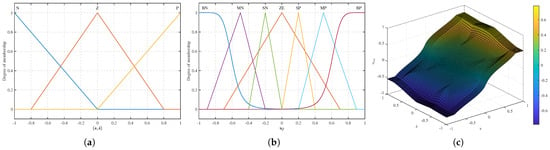
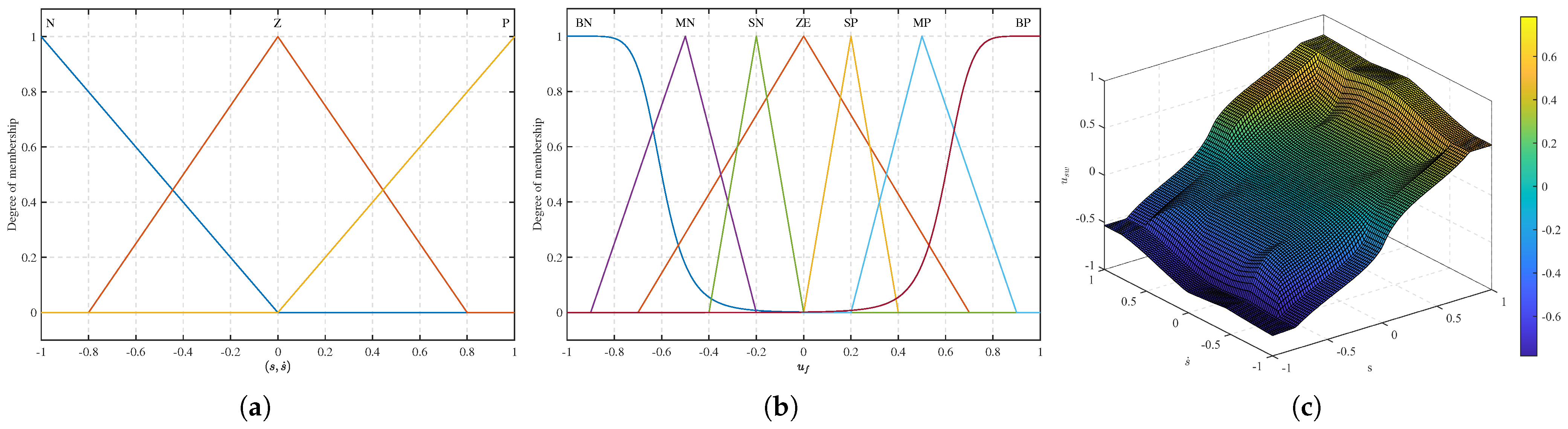
Figure 8a presents triangular-type inputs, whereas Figure 8b illustrates the output membership functions. Figure 8c shows the results inferred from fuzzy rules. Modulating the boundary layer thickness involves adjusting the range of fuzzy sets Z and ZE in both the input and output, allowing for variations in two distinct steps.

Figure 8. (a) Input and (b) output membership functions, and (c) combined 3-D plot of input and output membership functions.

The focus variation in the boundary layer thickness is modified by the proposed fuzzy system with the saturation function in two steps. First, the slope of the saturation function is systematically varied to achieve optimal performance of the fixed-boundary-layer fractional-order super-twisting sliding mode controller (FOSTSMC). The parameters “ZE” and “Z” are then tuned so that the boundary layer thickness obtained in the first step matches the desired one. After these modifications, the specified boundary-layer value ($\psi$) in this paper is 0.8. A Mamdani-type fuzzy inference approach was adopted to satisfy the resource constraints of robustness, enhanced tracking performance, improved system stability, and chattering suppression. This approach is based on a rule–based matrix with 9 fuzzy rules as shown in the Table 4.

Table 4. Rules matrix in terms of s and $\dot{s}$ after swapping these variables s and $\dot{s}$. Abbreviations: N = Negative, P = Positive, ZE = (Output) Zero, SP = Small Positive, BP = Big Positive, Z = (Input) Zero, MP = Medium Positive, BN = Big Negative, MD = Medium (output), SN = Small Negative.

Switching Variable, s	Alteration in Switching Variable, $\dot{\mathit{s}}$
	N	Z	P
N	BN	BN	MD
Z	SN	ZE	SP
P	MP	BP	BP

4.4. Stability and Convergence Analysis

To rigorously establish the stability and convergence properties of the closed-loop PMSG-WECS under the proposed Fuzzy-FOSTSMC, we present a complete Lyapunov-based analysis grounded in fractional-order calculus and adaptive control theory.

4.4.1. Lyapunov Function for Neural Estimation Subsystem

Define the composite Lyapunov candidate function as

$$V\left(t\right)={\displaystyle \frac{1}{2}}{s}^2+{\displaystyle \frac{1}{2{\gamma }_1}}{\tilde{W}}_{L_f^{2}h}^T{\tilde{W}}_{L_f^{2}h}+{\displaystyle \frac{1}{2{\gamma }_2}}{\tilde{W}}_{L_g{L}_{f}h}^T{\tilde{W}}_{L_g{L}_{f}h},$$

where s is the fractional-order sliding surface defined in Equation (62), $\tilde{W}=W-\widehat{W}$ denotes the neural weight estimation error, and ${\gamma }_1,{\gamma }_2>0$ are positive adaptation gains.

Using the property of the Caputo fractional derivative [Lemma 1],

$$D^{\overline{\gamma }}\left({\displaystyle \frac{1}{2}}{x}^2\right)\le x{D}^{\overline{\gamma }}x,0<\overline{\gamma }<1,$$

The fractional derivative of $V\left(t\right)$ satisfies

$$D^{\overline{\gamma }}V\le s{D}^{\overline{\gamma }}s-{\displaystyle \frac{1}{{\gamma }_1}}{\tilde{W}}_{L_f^{2}h}^T{D}^{\overline{\gamma }}{\widehat{W}}_{L_f^{2}h}-{\displaystyle \frac{1}{{\gamma }_2}}{\tilde{W}}_{L_g{L}_{f}h}^T{D}^{\overline{\gamma }}{\widehat{W}}_{L_g{L}_{f}h}$$

From Equation (63), the dynamics of the sliding surface yield:

$$D^{\overline{\gamma }}s=c_1{D}^{2-\gamma }e+c_2\mu (\mu -1){\left|e\right|}^{\mu -2}\left({\widehat{L}}_f^{2}h\left(x\right)+{\widehat{L}}_g{L}_{f}h\left(x\right)u-{\ddot{z}}_{1,\mathrm{ref}}\right)$$

Substituting the control law (Equation (67)) and using the definitions of the estimation errors (Equation (54)), we obtain:

$$D^{\overline{\gamma }}s=-k_1{\left|s\right|}^{1/2}{u}_f-k_2{\int }_0^t{u}_f\left(\tau \right)d\tau +\rho ,$$

where $\rho =\Xi +\delta$ aggregates the effects of the neural approximation error and higher-order modeling uncertainty and is bounded by the assumption.

Now, select the fractional-order weight update laws as

$$D^{\overline{\gamma }}{\widehat{W}}_{L_f^{2}h}={\gamma }_{1}sh\left(x\right),D^{\overline{\gamma }}{\widehat{W}}_{L_g{L}_{f}h}={\gamma }_{2}suh\left(x\right).$$

Substituting into $D^{\overline{\gamma }}V$ and using $\tilde{W}=W-\widehat{W}$, the cross terms cancel, yielding

$$D^{\overline{\gamma }}V\le -k_1{\left|s\right|}^{3/2}-k_2\left|s\right|{\int }_0^t\left|s\left(\tau \right)\right|d\tau +(\rho +\Xi )\left|s\right|.$$

For sufficiently large gains $k_1,k_2>0$ such that

$$k_1{\left|s\right|}^{1/2}+k_2{\int }_0^t\left|s\left(\tau \right)\right|d\tau >\rho +\Xi ,$$

we have $D^{\overline{\gamma }}V<0$ for all $s\ne 0$. Thus, $V\left(t\right)$ is strictly decreasing, and all signals are bounded.

4.4.2. Finite-Time Convergence of Sliding Dynamics

Consider the reduced Lyapunov function $V_s={\displaystyle \frac{1}{2}}{s}^2$. The Caputo derivative satisfies

$$D^{\overline{\gamma }}{V}_s\le s{D}^{\overline{\gamma }}s\le -k_1{\left|s\right|}^{3/2}-k_2\left|s\right|{\int }_0^t\left|s\left(\tau \right)\right|d\tau +\rho \left|s\right|$$

Because $u_f\in [-1,1]$ and mimics $\mathrm{sign}\left(s\right)$ via the fuzzy boundary layer, and given the gain condition above, one can write

$$D^{\overline{\gamma }}{V}_s\le -\eta V_s^{3/4},\eta =\sqrt{2}{k}_1>0$$

According to Lemma 2, if $D^{\overline{\gamma }}V\le -\eta V^{\alpha }$ with $0<\alpha <1$ and $\eta >0$, then the system converges to the origin in a finite time T given by

$$T\le {\left[{\displaystyle \frac{V^{1-\alpha }\left(0\right)}{\eta (1-\alpha )}}\right]}^{1/\overline{\gamma }}$$

Here, $\alpha =3/4<1$, so the finite-time convergence of $s\left(t\right)\to 0$ is guaranteed. This is because the sliding surface $s=0$ implies $e=0$, the tracking error converges to zero in a finite time. Thus, the closed-loop system achieves finite-time stability rather than merely asymptotic convergence.

Under Assumptions 1–4, the proposed Fuzzy-FOSTSMC ensures

• Boundedness of all closed-loop signals,
• Finite-time convergence of the tracking error to zero,
• Chattering-free control via adaptive fuzzy boundary layer,
• Robustness against parametric uncertainties and external disturbances.

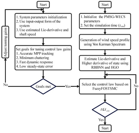
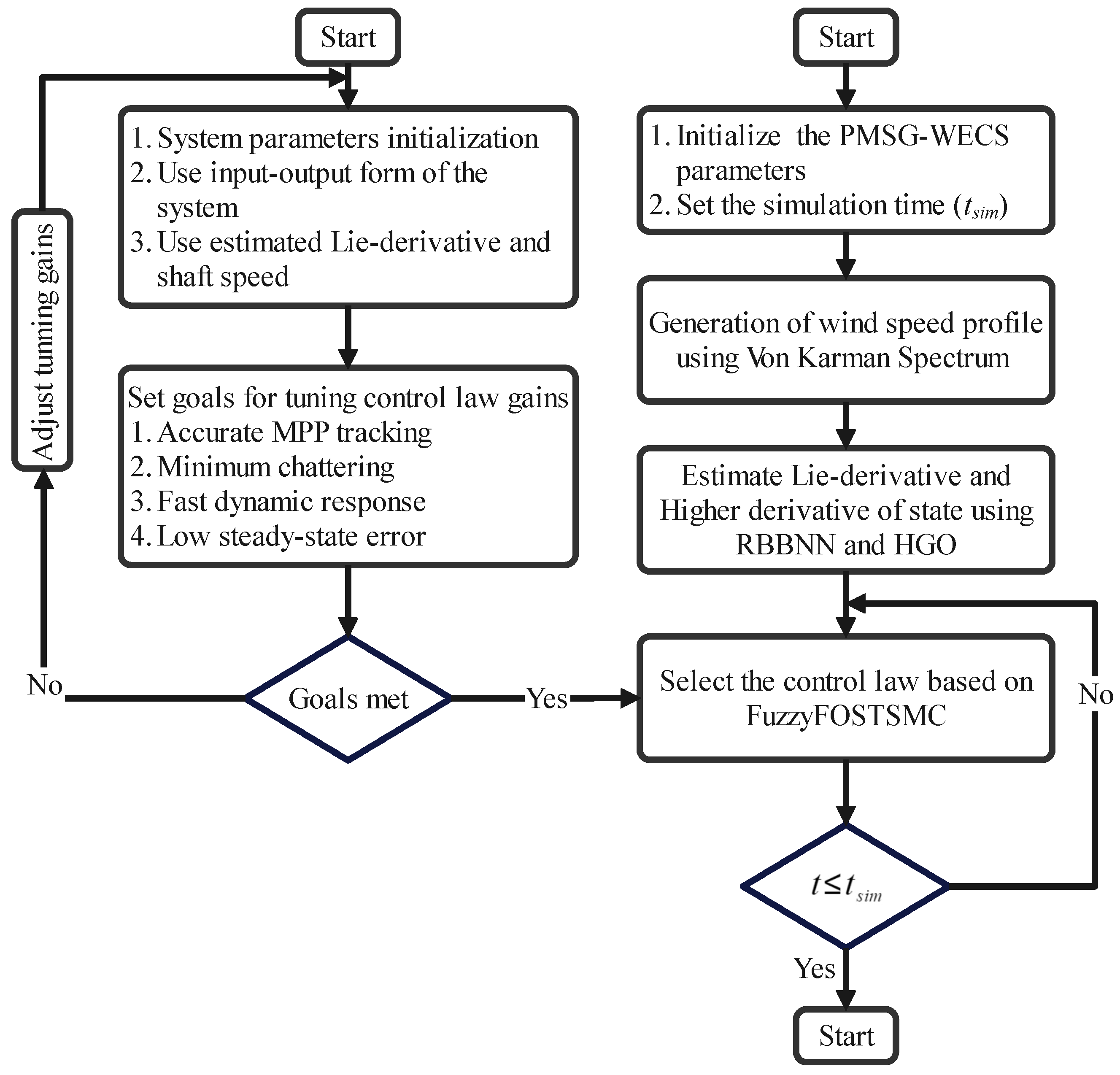
A key benefit of the finite-time sliding mode surface design presented in this study is its ability to ensure faster and more reliable convergence than traditional SMC methods. Conventional SMC algorithms typically take longer to converge (approach equilibrium), which may be unsuitable for applications that require an immediate response (such as wind energy systems). The block diagram describing the proposed control scheme is shown in Figure 9, and the computational flow diagram of the entire system is shown in Figure 10.

Figure 9. Block diagram of the proposed neuro-adaptive Fuzzy-FOSTSMC-based MPPT control architecture.

Figure 10. Computational flowchart showing the methodology of realization in real-time of the control law.

5. Simulation Results and Discussion

The effectiveness of the proposed neuro-adaptive Fuzzy-FOSTSMC for power maximization in WECS is investigated through simulation studies. The simulations are performed in MATLAB/Simulink R2023a employing a fixed-step ode4 (Runge–Kutta) integration method. The performance of the proposed approach is evaluated against several benchmark control strategies, namely classical sliding mode control (CSMC), fractional-order sliding mode control [32], super-twisting sliding mode control, and fractional-order super-twisting sliding mode control [47]. Simulation studies are performed on a standalone 3 kW WECS, comprising a fixed-pitch, variable-speed PMSG with an integrated front-end for power control. A 100-s wind profile at 2.0 m/s is applied while the turbine operates in fixed-pitch, variable-speed mode. All our benchmark controllers are tuned the same way for a fair comparison. The gains are iteratively tuned for performance with stability and are given in Table 5.

Table 5. Controller parameters.

Controllers	Parameters and Values
CSMC	$c=150$, $k=40$
FOSMC	$c_1=0.5$, $c_2=6$, $\gamma =0.6$, $\mu =0.9$, $k=20$
STSMC	$c=100$, $k_1=10$, $k_2=15$
FOSTSMC	$c_1=0.6$, $c_2=4$, $\gamma =0.6$, $\mu =0.9$, $k_1=12$, $k_2=30$
Fuzzy-FOSTSMC	$c_1=0.2$, $c_2=7$, $\gamma =0.6$, $\mu =0.9$, $k_1=15$, $k_2=40$

5.1. Simulation Results of the RBFNN

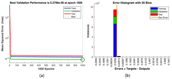
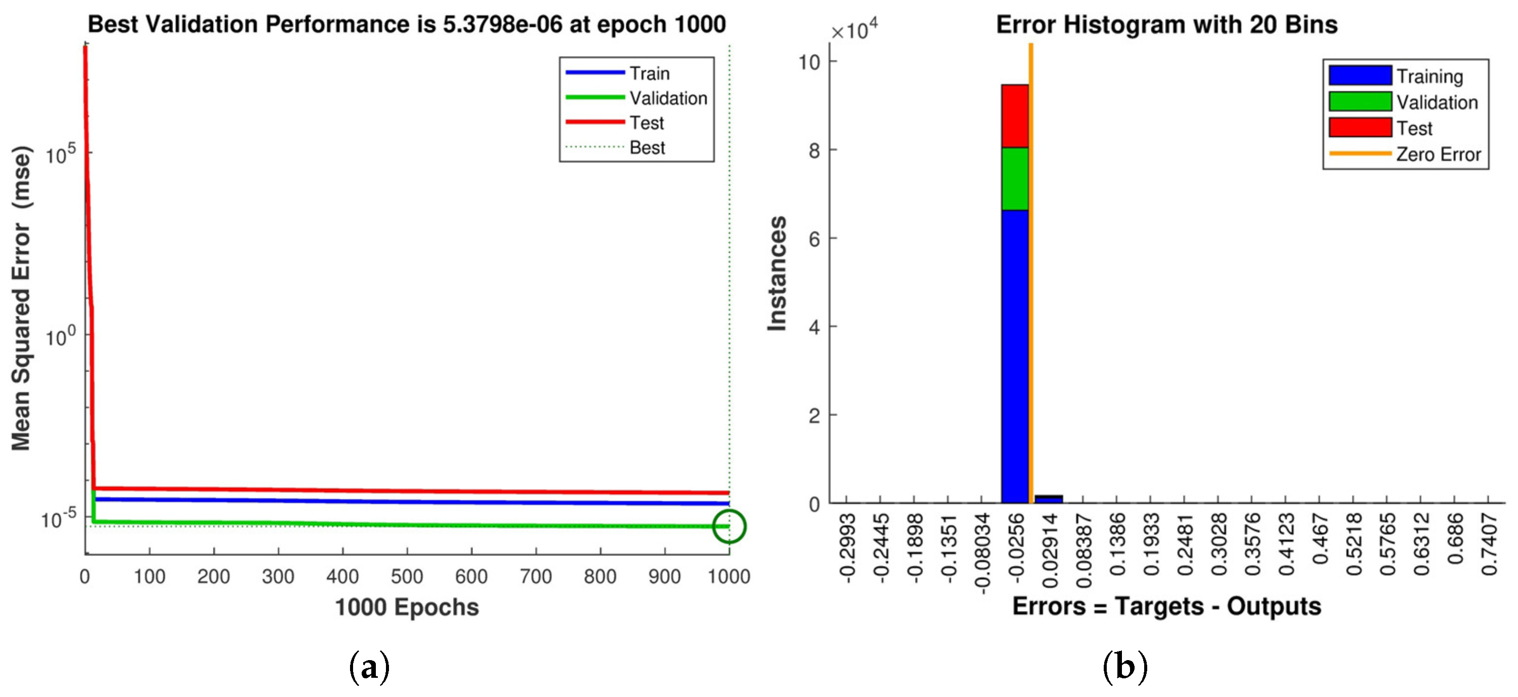
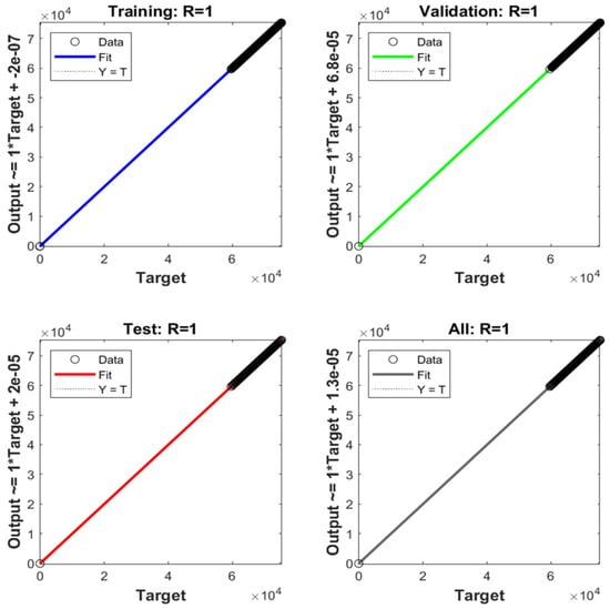
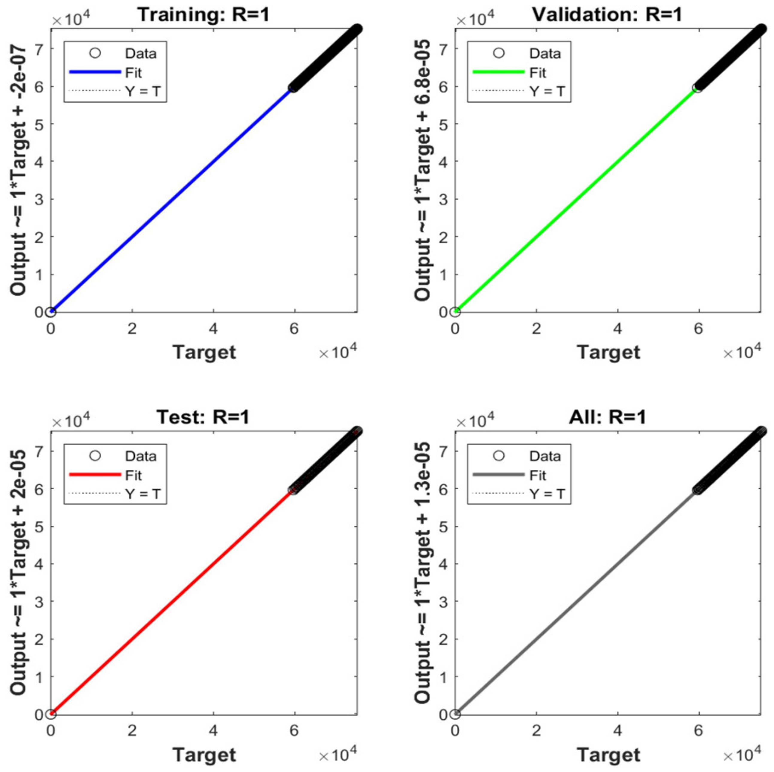
The performance of the radial basis function neural network in estimating the Lie derivatives $L_f^{2}h\left(x\right)$ and $L_g{L}_{f}h\left(x\right)$ is evaluated through simulation results in this subsection. The performance assessment is carried out using the mean squared error obtained during the estimation process, as shown in Figure 11a. A relatively large initial error was observed, followed by a monotonic reduction across the training epochs, indicating progressive learning convergence. The distribution of estimation errors for both $L_f^{2}h\left(x\right)$ and $L_g{L}_{f}h\left(x\right)$ is further examined through the error histogram shown in Figure 11b. Scatter plots of the predicted outputs versus the corresponding target values are illustrated in Figure 12. The accuracy of the estimation is quantitatively evaluated by the regression coefficient (R), where values close to unity indicate a strong correlation and high estimation accuracy, and lower values correspond to degraded approximation performance.

Figure 11. (a) Performance function of radial basis function neural network and (b) Error histogram.

Figure 12. Regression plot of radial basis function neural network.

5.2. Simulation Results of the State Estimator

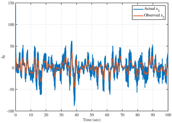
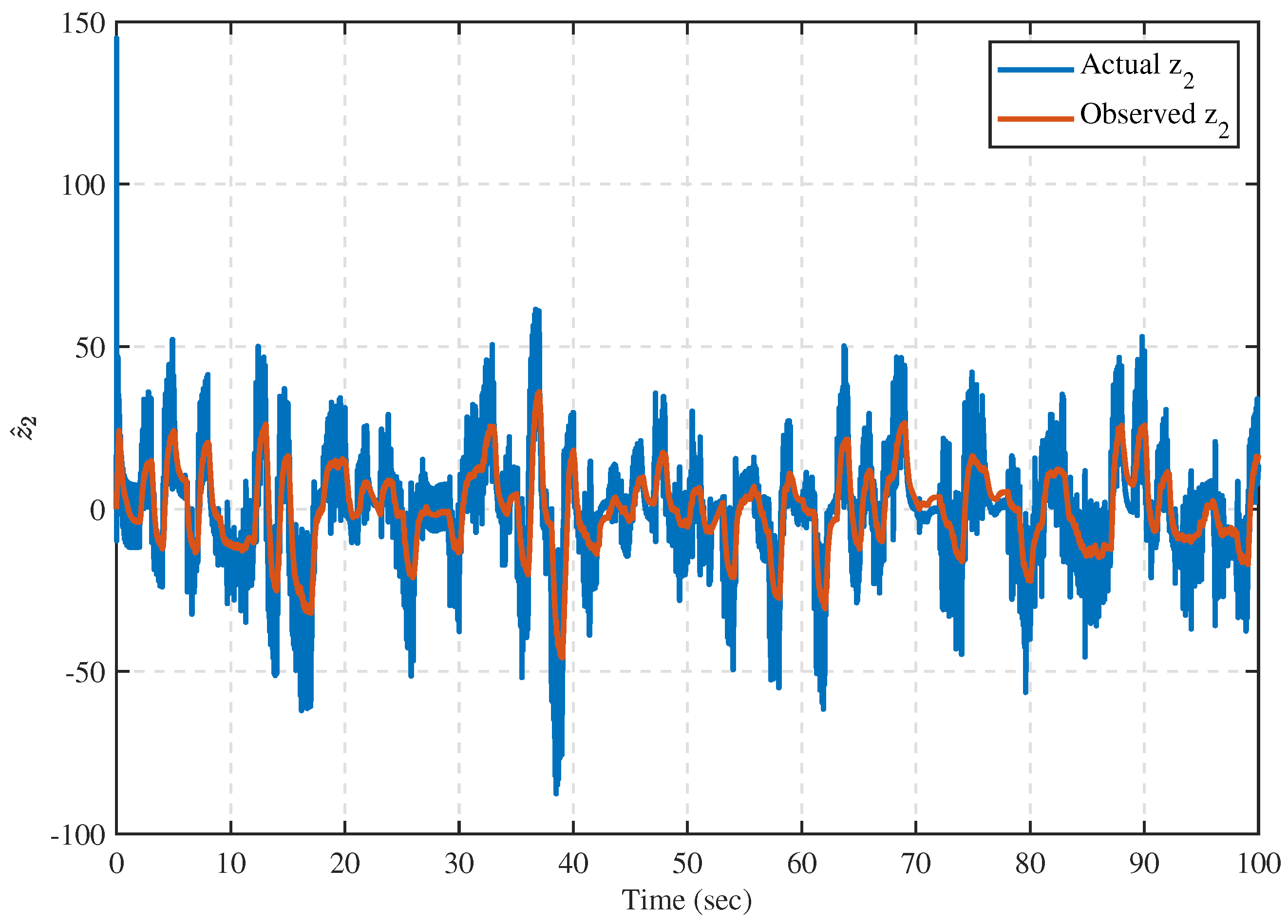
The stability of the closed-loop system relies on the fast convergence of the proposed observer. Such convergence is achieved through an appropriate bound on the high-gain parameter $ϵ$, as established in [48] and the related HGO literature. Notably, our simulations consistently employed a high-gain observer. The primary disparity between the classical observer and high-gain observer lies in the behavior of the gain parameter $ϵ$. In contrast to a classical observer, in a high-gain observer, $ϵ$ does not necessarily converge to zero. The reason for selecting the high-gain observer is to satisfy the asymptotic stability requirement of the overall closed-loop system. Moreover, the proposed differentiator can also estimate the unmeasured states, as shown in Figure 13.

Figure 13. Actual and estimated values of $z_2$.

5.3. Result Comparison of Proposed Controller

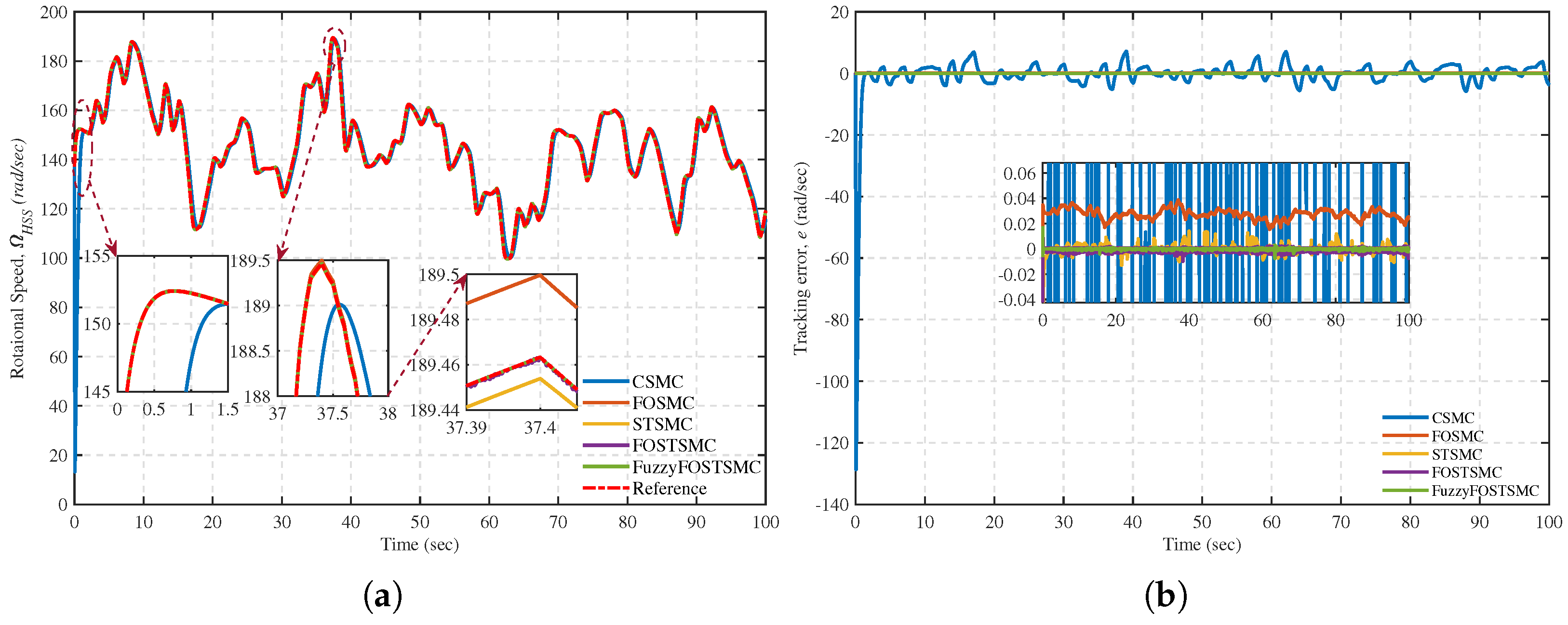
This section presents a comparative performance evaluation of the proposed Fuzzy-FOSTSMC with the conventional CSMC, FOSMC [32], STSMC, and FOSTSMC [47]. Graphical results are used to compare the system responses obtained using the Fuzzy-FOSTSMC and standard FOSTSMC. The analysis aims to demonstrate the performance enhancement achieved by the proposed Fuzzy-FOSTSMC scheme.

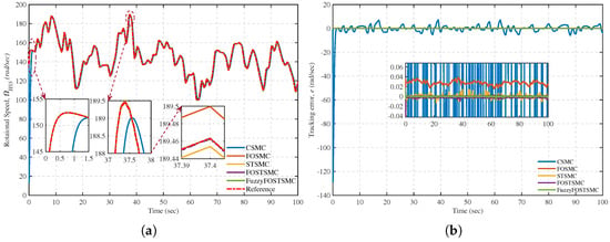
Figure 14a illustrates a comparative analysis of the wind shaft speed tracking performance of the PMSG using various control methodologies. The results show that Fuzzy-FOSTSMC outperforms other control methods, such as CSMC, FOSMC, STSMC, and FOSTSMC, especially when magnified locally. This superiority highlights the outstanding wind-speed tracking performance of Fuzzy-FOSTSMC. In addition, the Fuzzy-FOSTSMC controller exhibits finite-time convergence and enables stable, accurate tracking of the wind shaft speed. This property verifies that Fuzzy-FOSTSMC can guarantee reliable and accurate control performance when applied to practical wind energy systems.

Figure 14. (a) High -speed shaft angular speed tracking performance and (b) associated tracking deviation.

Considering the tracking response of the PMSG wind shaft speed, from Figure 14b, the accuracy of the Fuzzy-FOSTSMC controller is better than that of the CSMC, FOSMC, STSMC, and FOSTSMC controllers. This shows the robustness of the Fuzzy-FOSTSMC controller against initial noise and its finite-time convergence.

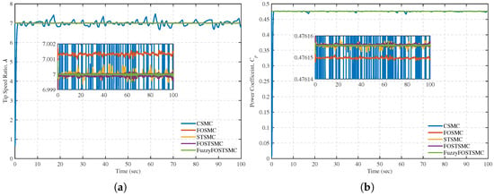
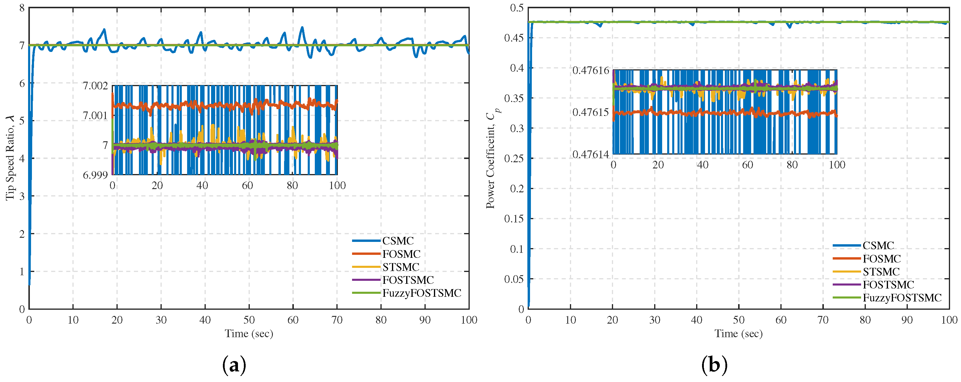
Additionally, the Fuzzy-FOSTSMC can track the VSWT TSR as shown in Figure 15a with few jitters around the optimal TSR (${\lambda }_{opt}$). This feature of the Fuzzy-FOSTSMC controller also makes it the most suitable for an MPPT controller. A plot of the power conversion factor ($C_p$) of the controllers is presented in Figure 15b. Under the designated wind speed profile, the proposed Fuzzy-FOSTSMC scheme achieves good tracking of the maximum $C_p$ value ($C_{pmax}=0.4762$), ensuring high power extraction. In particular, the enlarged views in the above figures show small initial perturbations in the Fuzzy-FOSTSMC and demonstrate robust performance in the presence of uncertain disturbances. This robustness can be explained by the fact that in the Fuzzy-FOSTSMC, disturbances are rapidly attenuated, and during the initial control phase, the system exhibits minimal oscillation. On the other hand, controllers like the CSMC, FOSMC, STSMC, and FOSTSMC may exhibit more oscillatory behavior at the beginning due to disturbances and slower response dynamics.

Figure 15. (a) Tip speed ratio performance and (b) Power conversion coefficient.

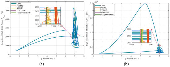
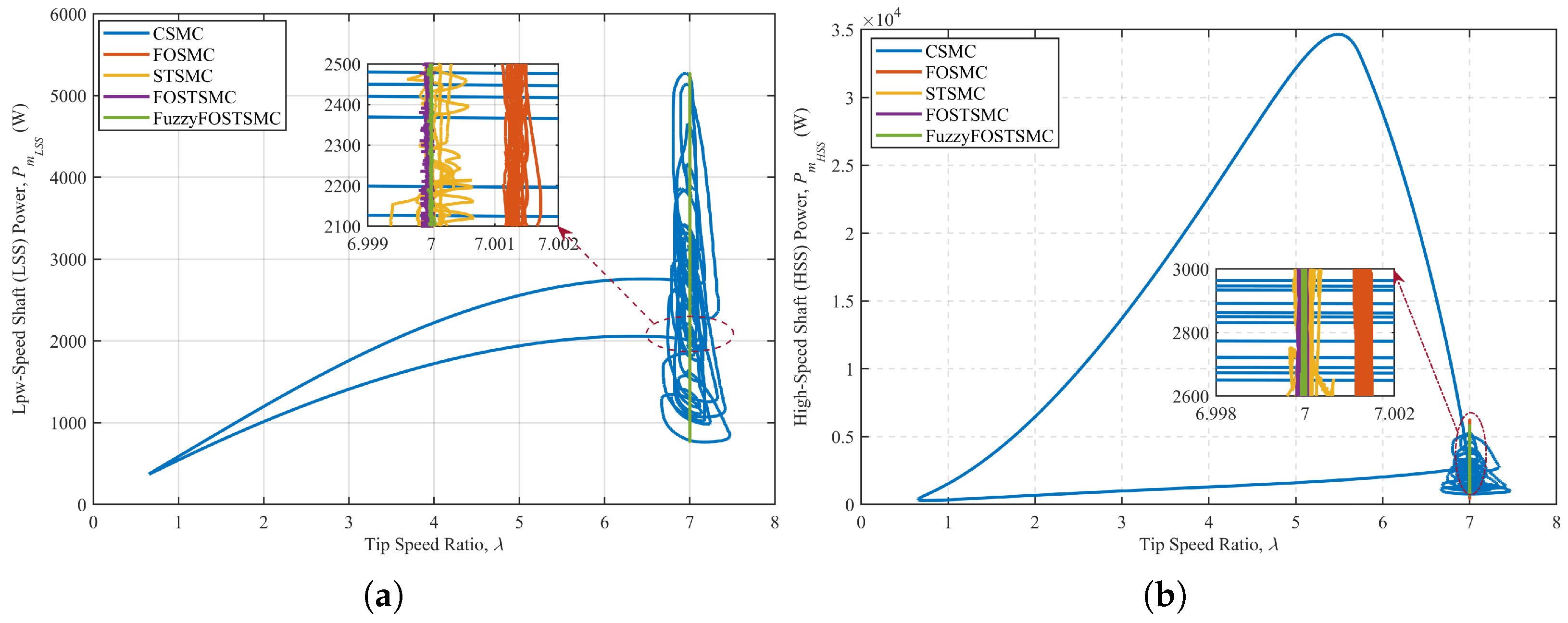
The mechanical power of the low-speed and high-speed shafts versus the tip-speed ratio is shown in Figure 16a and Figure 16b, respectively. By operating near the optimal tip-speed ratio, the Fuzzy-FOSTSMC controller preserves mechanical power at its desired level, resulting in improved system performance. However, the power fluctuations were quite large, indicating that FOSTSMC’s performance was poor. On the other hand, the performance of the STSMC, FOSMC, and CSMC controllers was inadequate, as evidenced by the large fluctuations in mechanical power. These oscillations reveal the limitations of these control schemes in producing a steady power output under varying load conditions.

Figure 16. Mechanical power as a function of the tip-speed ratio: (a) low-speed shaft and (b) high-speed shaft.

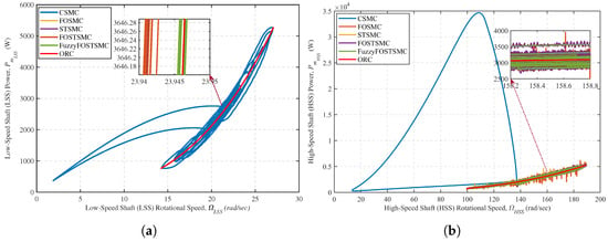
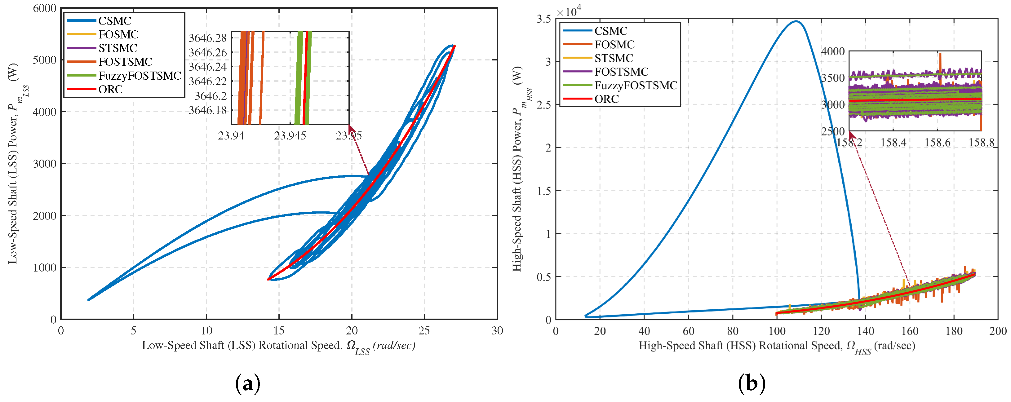
Figure 17a and Figure 17b present the mechanical power as a function of the rotational speed for the low-speed and high-speed shafts, respectively. The results demonstrate that the proposed Fuzzy-FOSTSMC-based MPPT controller effectively regulates the VSWT rotational speed within the desired operating region. The control is designed to maximize the power drawn from the system. In comparison, the FOSTSMC deviates from the Optimal Reference Curve (ORC), resulting in significant differences in both speed and energy. On the other hand, STSMC, FOSMC, and CSMC controllers exhibited large oscillations in speed and power, indicating that their performance is worse than that of the other two controllers. These results confirm that the Fuzzy-FOSTSMC MPPT controller can effectively track the maximum power in changing environments and ensure the VSWT operates under extreme working conditions, thereby achieving higher VSWT output power. This information is essential for the design of wind turbine systems to maximize energy output, an important factor for sustainable and efficient renewable energy generation.

Figure 17. Variation of output power as a function of rotational speed: (a) low-speed shaft and (b) high-speed shaft.

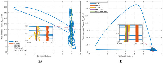
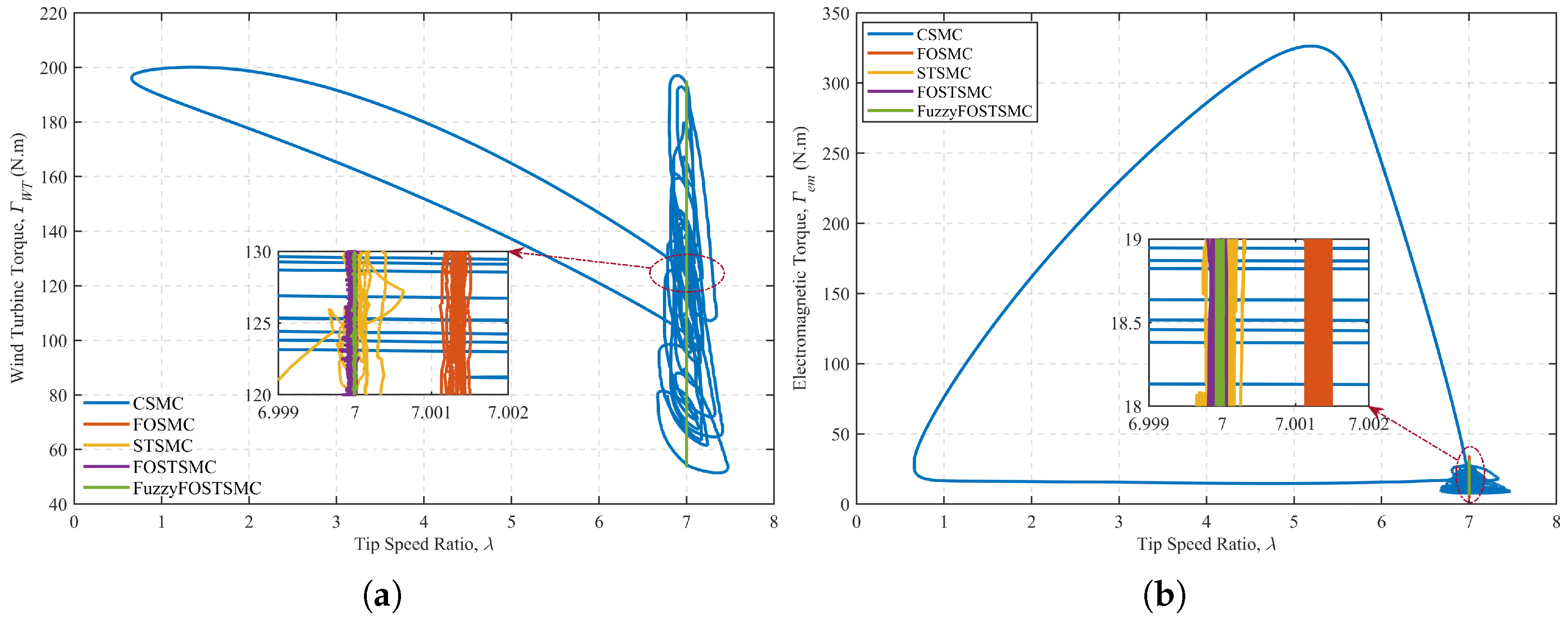
Figure 18a,b depict the variation of the PMSG electromagnetic torque with respect to the TSR. The inset highlights the capability of the Fuzzy-FOSTSMC to accurately track the electromagnetic torque corresponding to the optimal TSR, ensuring maximum power extraction. This control method demonstrates its feasibility for guaranteeing maximum power point operation of a PMSG under high-power conditions. The close correspondence between the controller output and the optimal TSR indicates the robustness and efficiency of the presented Fuzzy-FOSTSMC method in improving the PMSG system’s performance. By tracking the ideal operating point with the PMSG’s electromagnetic torque, the controller enhances the overall energy-conversion efficiency of the PMSG, which is important in many renewable energy applications.

Figure 18. Torque variation with respect to the tip-speed ratio (a) Wind turbine side and (b) generator side.

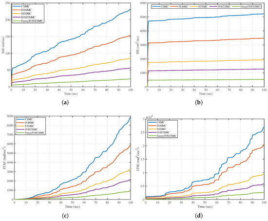
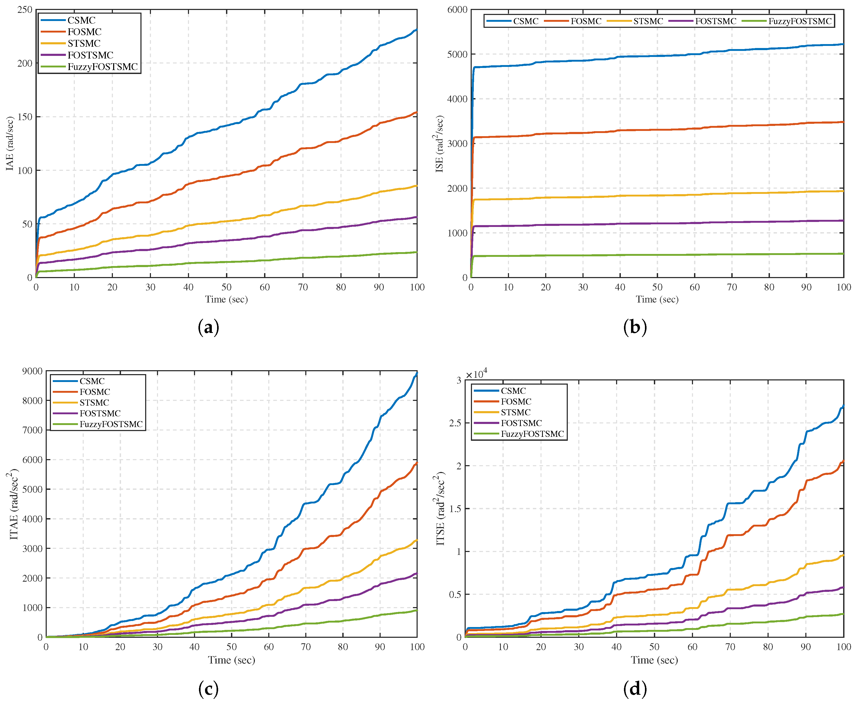
Moreover, the dynamic behavior of the MPPT scheme was quantitatively analyzed using four integral performance indices: IAE, ISE, ITAE, and ITSE. As summarized in Table 6 and shown in Figure 19, the proposed Fuzzy-FOSTSMC achieves the minimum total error at all times, indicating the fastest convergence rate, the least steady-state error, and best transient regulation among FOSTSMC, STSMC, FOSMC, and CSMC. These results confirm the aforementioned tracking capability, and the robustness of the proposed controller is validated in dynamic situations. Table 7 presents a quantitative comparison between the proposed MPPT scheme and other benchmark MPPT algorithms, indicating the best performance of the proposed scheme with respect to the main evaluation indices and global tracking quality.

Table 6. Performance indices.

Performance Indices	Controllers
	CSMC	FOSMC	STSMC	FOSTSMC	Fuzzy-FOSTSMC
IAE	230.974	153.982	85.546	56.262	23.516
ISE	5223.6	3481.07	1934.66	1273.76	532.82
ITAE	8943.37	5890.97	3297.32	2159.95	906.203
ITSE	26,846.5	20,547.1	9546.64	5830.6	2695.64

Figure 19. Comparison of performance indices (a) IAE, (b) ISE, (c) ITAE, and (d) ITSE.

Table 7. Quantitative comparison between the proposed MPPT scheme and benchmark MPPT methods.

Performance Metrics	Controllers
	CSMC	FOSMC	STSMC	FOSTSMC	Fuzzy-FOSTSMC
System Type	PMSG-WECS	PMSG-WECS	PMSG-WECS	PMSG-WECS	PMSG-WECS
Settling Time (s)	2.8	2.5	1.9	1.6	1.2
Rise Time (s)	1.1	0.9	0.7	0.6	0.4
Overshoot (%)	8.5	6.2	3.1	1.8	0.3
Steady-State Error (rad/s)	12.3	8.7	4.2	2.1	0.018
Tracking Accuracy (%)	92.1	94.3	96.8	98.2	99.96
Overall Efficiency (%)	94.2	95.8	96.9	97.4	99.99

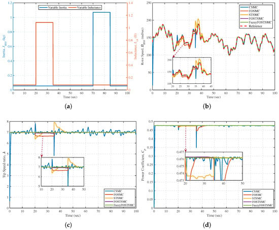
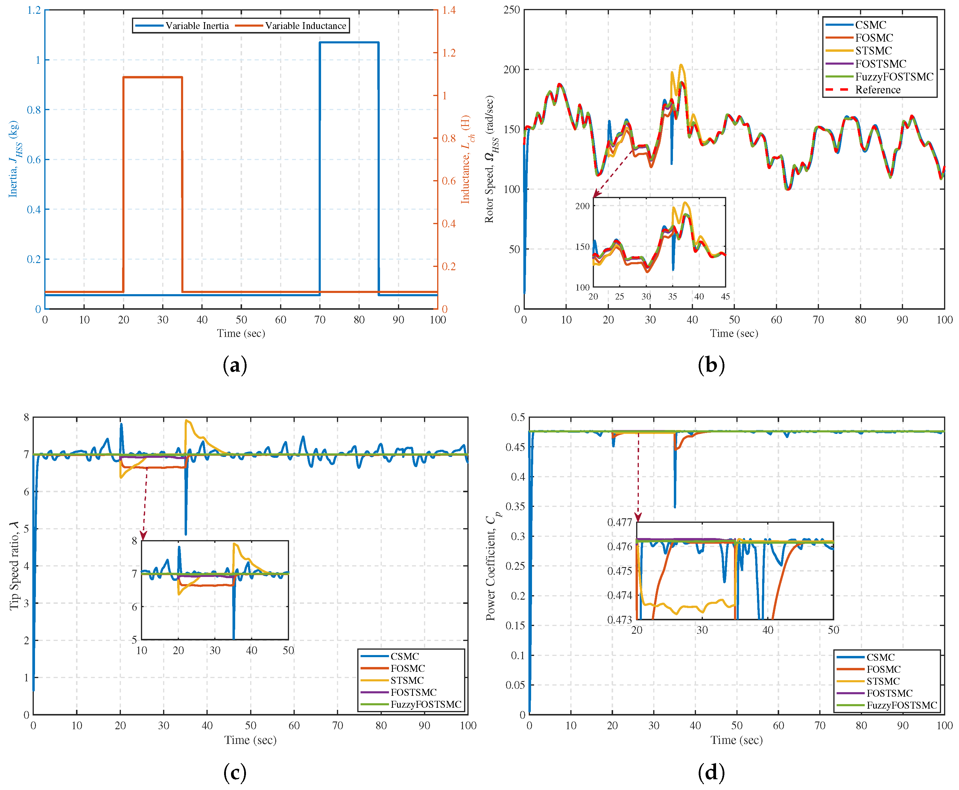
The stability and tracking performance of the proposed MPPT under significant parametric uncertainties are investigated. Figure 20a shows the applied ±30% step variations in high-speed shaft inertia $J_{hss}$ and chopper inductance $L_{ch}$. The comparisons reveal (see Figure 20b) that the Fuzzy-FOSTSMC maintains high accuracy in rotor speed regulation with a maximum transient error of less than 2 rad/s, and it recovers in 0.8 s after each disturbance.

Figure 20. Comparison analysis under the influence of parametric variation (a) Varying inertia and inductance, (b) Speed tracking, (c) TSR, and (d) Power coefficient.

The steady-state tracking error remains within ±0.02 rads/s over the full operating space, indicating that the mechanical and electrical parameter mismatch has strong robustness. On the other hand, the CSMC controller exhibits significant overshoot (>15 rad/s) and persistent oscillations after parameter changes, whereas the FOSMC and STSMC controllers are only mildly affected. Although the FOSTSMC improves transient performance, residual drift (5 rad/s) persists due to the nominal plant dynamics. Improved speed tracking directly improves aerodynamic performance. As shown in Figure 20c, the achieved controller maintains the power coefficient $C_p$ at about 0.4761–0.4762, equivalent to a deviation from the optimal value less than 0.02% under all disturbances. In contrast, CSMC, FOSMC, STSMC, and FOSTSMC undergo significant reductions in $C_p$, especially at inertia changes, meaning the torque dynamics are partially compensated. On the other hand, the tip-speed ratio (Figure 20d) is well controlled at ($\lambda$ = 7.000 ± 0.002) in Fuzzy FOSTSMC. In contrast, other controllers show some oscillations ($\lambda \approx$ 6.95–7.08), which represent a transient loss of optimal operating conditions. This behavior indicates that the RBFNN-based online estimation of higher-order Lie derivatives $L_g{L}_{f}h\left(x\right)$ and $L_f^{2}h\left(x\right)$ can successfully eliminate modeling uncertainties and maintain mechanical–electrical coupling coherence. To sum up, these cooperative features in the fractional-order super-twisting structure, fuzzy smoothing technique, and adaptive neural estimation scheme allow an agile disturbance elimination for a persistent MPPT precision in the presence of practical parameter variations, outperforming traditional and then advanced SMC-based algorithms.

The comparative analysis confirmed the superior performance of the proposed Fuzzy-FOSTSMC over the CSMC, FOSMC, STSMC, and conventional FOSTSMC. The controller achieves high-accuracy wind-speed tracking, suppresses power oscillations, ensures smooth torque regulation, and improves energy conversion efficiency. It consistently outperformed competing methods across key MPPT indicators, including $C_p$ tracking, mechanical power at low and high speeds, rotor-speed regulation, and electromagnetic torque control. These results demonstrate an enhanced energy capture capability and improved system stability, establishing the Fuzzy-FOSTSMC as a high-performance MPPT solution for wind energy conversion systems.

6. Conclusions, Limitations and Future Direction

This study presents a neuro-adaptive fuzzy fractional-order super-twisting sliding mode control strategy integrated with a high-gain observer and radial basis function neural network for maximum power point tracking in a standalone PMSG-based WECS. The proposed framework eliminates chattering, operates under output feedback (using only rotor speed measurement), and compensates for model uncertainties without requiring exact system dynamics. Comprehensive MATLAB/Simulink simulations demonstrated that the controller achieved a tracking accuracy of 99.96% with a steady-state speed error of merely 0.018 rad/s, significantly outperforming the conventional CSMC, FOSMC, STSMC, and FOSTSMC. It reduces the integral absolute error by 58.2% from 56.262 to 23.516 and exhibits a settling time of 1.2 s with only a 0.3% overshoot. Critically, under ±30% parametric variations in the high-speed shaft inertia $J_{hss}$ and chopper inductance $L_{ch}$, the system maintains the power coefficient at $C_p=0.4762$ (optimal value) with less than 0.02% deviation and regulates the tip-speed ratio within $\lambda =7.000\pm 0.002$. These quantitative results confirm that the proposed approach not only ensures robust, chattering-free control but also maximizes aerodynamic power extraction under uncertain operating conditions. Consequently, the Fuzzy-FOSTSMC framework offers a high-performance, model-free, and practically viable solution for next-generation variable-speed WECS.

Despite promising simulation results, this study has notable limitations: (a) all validations are conducted in idealized MATLAB/Simulink environments without measurement noise or quantization effects; (b) the RBFNN and fractional-order operators impose a significant computational load that may challenge real-time deployment on standard DSPs; (c) the high-gain observer’s sensitivity to sensor noise remains untested; and (d) no hardware validation has been performed.

Future efforts will focus on three fronts: (1) hardware-in-the-loop validation using OPAL-RT to assess real-time feasibility and noise robustness; (2) FPGA implementation of the fractional-order operator and fuzzy logic block to evaluate computational footprint; and (3) experimental testing on our lab-scale 3 kW PMSG-WECS testbench to quantify energy yield improvement over a 30-day wind profile.

References

- Ullah, A.; Ullah, S.; Rahman, T.U.; Sami, I.; Rahman, A.U.; Alghamdi, B.; Pan, J. Enhanced wind energy conversion system performance using fast smooth second-order sliding mode control with neuro-fuzzy estimation and variable-gain robust exact output differentiator. Appl. Energy 2025, 377, 124364. [Google Scholar] [CrossRef] [Scilit]
- Ashraf, H.; Abdellatif, S.O.; Elkholy, M.M.; El-Fergany, A.A. Computational techniques based on artificial intelligence for extracting optimal parameters of PEMFCs: Survey and insights. Arch. Comput. Methods Eng. 2022, 29, 3943–3972. [Google Scholar] [CrossRef] [Scilit]
- Valavanidis, A. Global Electricity Generation from Renewable Sources. Journal 2016, 2, 99–110. [Google Scholar]
- Sang, L.Q.; Li, Q.; Cai, C.; Maeda, T.; Kamada, Y.; Wang, X.; Zhou, S.; Zhang, F. Wind tunnel and numerical study of a floating offshore wind turbine based on the cyclic pitch control. Renew. Energy 2021, 172, 453–464. [Google Scholar] [CrossRef] [Scilit]
- Benbouhenni, H.; Hamza, G.; Oproescu, M.; Bizon, N.; Thounthong, P.; Colak, I. Application of fractional-order synergetic-proportional integral controller based on PSO algorithm to improve the output power of the wind turbine power system. Sci. Rep. 2024, 14, 609. [Google Scholar] [CrossRef] [Scilit]
- Rekioua, D. Power Electronics Used in WECS. In Wind Power Electric Systems; Springer: Berlin/Heidelberg, Germany, 2024; pp. 121–151. [Google Scholar]
- Kadhim, I.J.; Hasan, M.J. Enhancing power stability and efficiency with multilevel inverter technology based on renewable energy sources. Electr. Power Syst. Res. 2024, 231, 110290. [Google Scholar] [CrossRef] [Scilit]
- Maurya, V.K.; Pandey, J.; Gaur, C.; Singh, S. Original Research Article Design analysis of intelligent controller to minimize harmonic distortion and power loss of wind energy conversion system (grid connected). J. Auton. Intell. 2024, 7, 1–16. [Google Scholar]
- Yesudhas, A.A.; Joo, Y.H.; Lee, S.R. Reference model adaptive control scheme on PMVG-based wecs for MPPT under a real wind speed. Energies 2022, 15, 3091. [Google Scholar] [CrossRef] [Scilit]
- Shawqran, A.M.; El-Marhomy, A.; Sameh, M.A.; Attia, M.A. Comparative study of blade angle controllers with different optimization algorithms. Alex. Eng. J. 2022, 61, 3897–3912. [Google Scholar] [CrossRef] [Scilit]
- Mousa, H.H.; Youssef, A.R.; Mohamed, E.E. State of the art perturb and observe MPPT algorithms based wind energy conversion systems: A technology review. Int. J. Electr. Power Energy Syst. 2021, 126, 106598. [Google Scholar] [CrossRef] [Scilit]
- Fekkak, B.; Menaa, M.; Loukriz, A.; Kouzou, A. Control of grid-connected PMSG-based wind turbine system with back-to-back converters topology using a new PIL integration method. Int. Trans. Electr. Energy Syst. 2021, 31, e12882. [Google Scholar] [CrossRef] [Scilit]
- Mendi, B.; Pattnaik, M.; Srungavarapu, G. A single current sensor based adaptive step size MPPT control of a small scale variable speed wind energy conversion system. Appl. Energy 2024, 357, 122492. [Google Scholar] [CrossRef] [Scilit]
- Alhamdawee, R.; Hussain, M.M. A study of conventional and modern algorithms employed for MPPT in wind energy conversion systems: A review. In Proceedings of the 2024 3rd International conference on Power Electronics and IoT Applications in Renewable Energy and its Control (PARC), Mathura, India, 23–24 February 2024; IEEE: Piscataway, NJ, USA, 2024; pp. 14–23. [Google Scholar]
- Mourabit, Y.E.; Salime, H.; Bossoufi, B.; Motahhir, S.; Derouich, A.; Mobayen, S.; Zhilenkov, A. Enhanced Performance in PMSG-Based Wind Turbine Systems: Experimental Validation of Adaptive Backstepping Control Design. Energies 2023, 16, 7481. [Google Scholar] [CrossRef] [Scilit]
- Li, S.; Li, J.; Tang, Y.; Shi, Y.; Cao, W. Model-based model predictive control for a direct-driven permanent magnet synchronous generator with internal and external disturbances. Trans. Inst. Meas. Control 2020, 42, 586–597. [Google Scholar]
- AlGhamdi, S.; Hamdan, I.; Youssef, M.M.; Noureldeen, O. Development and application of fuzzy proportional-integral control scheme in pitch angle compensation loop for wind turbines. Machines 2021, 9, 135. [Google Scholar] [CrossRef] [Scilit]
- Zohra, A.F.; Khalil, B.I.; Slimane, L.; Youcef, S.; Benyounes, M. Artificial intelligence control applied in wind energy conversion system. Int. J. Power Electron. Drive Syst. 2018, 9, 571–578. [Google Scholar] [CrossRef] [Scilit]
- Hermassi, M.; Krim, S.; Kraiem, Y.; Hajjaji, M.A.; Mimouni, M.F.; Mtibaa, A. Wind speed estimation and maximum power point tracking using neuro-fuzzy systems for variable-speed wind generator. Wind Eng. 2024, 48, 1088–1104. [Google Scholar] [CrossRef] [Scilit]
- Perez-Perez, E.J.; Puig, V.; Lopez-Estrada, F.R.; Valencia-Palomo, G.; Santos-Ruiz, I.; Samada, S.E. Fault detection and isolation in wind turbines based on neuro-fuzzy qLPV zonotopic observers. Mech. Syst. Signal Process. 2023, 191, 110183. [Google Scholar] [CrossRef] [Scilit]
- Pérez-Pérez, E.J.; Puig, V.; López-Estrada, F.R.; Valencia-Palomo, G.; Santos-Ruiz, I.; Osorio-Gordillo, G. Robust fault diagnosis of wind turbines based on MANFIS and zonotopic observers. Expert Syst. Appl. 2024, 235, 121095. [Google Scholar] [CrossRef] [Scilit]
- Yu, L.; Huang, J.; Luo, W.; Chang, S.; Sun, H.; Tian, H. Sliding-mode control for PMLSM position control—A review. Actuators 2023, 12, 31. [Google Scholar] [CrossRef] [Scilit]
- Ali, A.; Khan, Q.; Ullah, S.; Waqar, A.; Hua, L.G.; Bouazzi, I.; Jun, L.J. High gain differentiator based neuro-adaptive arbitrary order sliding mode control design for MPE of standalone wind power system. PLoS ONE 2024, 19, e0293878. [Google Scholar] [CrossRef] [Scilit]
- Oliveira, T.R.; Hsu, L.; Nunes, E.V.L. Smooth sliding control to overcome chattering arising in classical SMC and super-twisting algorithm in the presence of unmodeled dynamics. J. Frankl. Inst. 2022, 359, 1235–1256. [Google Scholar] [CrossRef] [Scilit]
- Bellarbi, S.; Koussa, D.S.; Djoudi, A. Sliding mode control for PMSG-based wind power system. J. Phys. Conf. Ser. 2018, 1081, 012012. [Google Scholar] [CrossRef] [Scilit]
- Khan, U.H.; Khan, Q.; Khan, L.; Alam, W.; Ali, N.; Khan, I.; Nisar, K.S.; Khan, R.A. MPPT control paradigms for PMSG-WECS: A synergistic control strategy with gain-scheduled sliding mode observer. IEEE Access 2021, 9, 139876–139887. [Google Scholar] [CrossRef] [Scilit]
- Ullah, A.; Ullah, S.; Zhang, Z.; Pan, J. Smooth super-twisting sliding mode control design with high order super-twisting observer for speed tracking control of permanent magnet synchronous motor drive system. ISA Trans. 2025, 162, 227–242. [Google Scholar] [CrossRef] [Scilit]
- Dursun, E.H.; Kulaksiz, A.A. Second-order sliding mode voltage-regulator for improving MPPT efficiency of PMSG-based WECS. Int. J. Electr. Power Energy Syst. 2020, 121, 106149. [Google Scholar] [CrossRef] [Scilit]
- Ullah, A.; Khan, L.; Khan, Q.; Ahmad, S. Variable gain high order sliding mode control approaches for PMSG basedvariable speed wind energy conversion system. Turk. J. Electr. Eng. Comput. Sci. 2020, 28, 2997–3012. [Google Scholar] [CrossRef] [Scilit]
- Ullah, A.; Ullah, S.; Hussan, U.; Alghamdi, B.; Pan, J. Optimized Neuro-Adaptive Third-Order Sliding Mode Control with High-Gain Differentiator for Enhanced Photovoltaic System Performance: Simulation and Experimental Validation. IEEE J. Emerg. Sel. Top. Power Electron. 2025, 13, 5970–5989. [Google Scholar] [CrossRef] [Scilit]
- Alsafran, A.S.; Ullah, S.; Ullah, A.; Hafeez, G.; Babar, M.Z.; Alghamdi, B.; Algethami, A.A. A Robust Fractional-Order Nonsingular Terminal Sliding Mode Control With Deep Learning-Based Lie Derivative Estimation for Maximum Power Point Tracking in Wind Turbine. IEEE Access. 2025, 13, 127423–127435. [Google Scholar] [CrossRef] [Scilit]
- Ullah, N.; Ali, M.A.; Ibeas, A.; Herrera, J. Adaptive fractional order terminal sliding mode control of a doubly fed induction generator-based wind energy system. IEEE Access 2017, 5, 21368–21381. [Google Scholar] [CrossRef] [Scilit]
- Rhaili, S.E.; Abbou, A.; Marhraoui, S.; El Hichami, N.; Moutchou, R. Optimal Power Generation Control of 5-Phase PMSG Based WECS by Using Enhanced Fuzzy Fractional Order SMC. Int. J. Intell. Eng. Syst. 2022, 15, 572–583. [Google Scholar] [CrossRef] [Scilit]
- Ullah, N.; Sami, I.; Chowdhury, M.S.; Techato, K.; Alkhammash, H.I. Artificial intelligence integrated fractional order control of doubly fed induction generator-based wind energy system. IEEE Access 2020, 9, 5734–5748. [Google Scholar] [CrossRef] [Scilit]
- Wu, A.; Zhao, B.; Mao, J.; Wu, G.; Zhang, X. Extended state observer based integral sliding model control for PMSG variable speed wind energy conversion system. In Proceedings of the 2015 34th Chinese Control Conference (CCC), Hangzhou, China, 28–30 July 2015; IEEE: Piscataway, NJ, USA, 2015; pp. 3387–3391. [Google Scholar]
- Rhaili, S.E.; Abbou, A.; El Hichami, N.; Marhraoui, S.; Chojaa, H. Maximum power extraction of five-phase PMSG based WECS by adopting an improved fractional order sliding mode strategy. OSF 2021, 40, 55–74. [Google Scholar] [CrossRef]
- Yessef, M.; Bossoufi, B.; Taoussi, M.; Lagrioui, A.; Chojaa, H. Overview of control strategies for wind turbines: ANNC, FLC, SMC, BSC, and PI controllers. Wind Eng. 2022, 46, 1820–1837. [Google Scholar] [CrossRef] [Scilit]
- Ntuli, W.K. Performance Evaluation of Control Strategies for Grid Connected Wind Power Generator. Ph.D. Thesis, Durban University of Technology (DUT), Durban, South Africa, 2023. [Google Scholar]
- Xue, D.; Bai, L. Introduction to Fractional Calculus. In Fractional Calculus: High-Precision Algorithms and Numerical Implementations; Springer: Berlin/Heidelberg, Germany, 2024; pp. 1–17. [Google Scholar]
- Ullah, S.; Alghamdi, H.; Algethami, A.A.; Alghamdi, B.; Hafeez, G. Robust Control Design of Under-Actuated Nonlinear Systems: Quadcopter Unmanned Aerial Vehicles with Integral Backstepping Integral Terminal Fractional-Order Sliding Mode. Fractal Fract. 2024, 8, 412. [Google Scholar] [CrossRef] [Scilit]
- Baleanu, D. New treatise in fractional dynamics. In Complex Systems: Fractionality, Time-Delay and Synchronization; Springer: Berlin/Heidelberg, Germany, 2011; pp. 1–41. [Google Scholar]
- Ullah, S.; Alsafran, A.S.; Harrison, A.; Hafeez, G.; Hassan, A.; Alghamdi, B.; Kraiem, H. A Uniform Robust Exact Differentiator based Neuro-Fuzzy Fractional Order Sliding Mode Control for Optimal Standalone Solar Photovoltaic System. IEEE Access 2025, 13, 4411–4423. [Google Scholar] [CrossRef] [Scilit]
- Kilbas, A.A.; Srivastava, H.M.; Trujillo, J.J. Theory and Applications of Fractional Differential Equations; Elsevier: Amsterdam, The Netherlands, 2006; Volume 204. [Google Scholar]
- Zholtayev, D.; Rubagotti, M.; Do, T.D. Adaptive super-twisting sliding mode control for maximum power point tracking of PMSG-based wind energy conversion systems. Renew. Energy 2022, 183, 877–889. [Google Scholar] [CrossRef] [Scilit]
- Cutululis, N.A.; Ceanga, E.; Hansen, A.D.; Sørensen, P. Robust multi-model control of an autonomous wind power system. Wind Energy Int. J. Prog. Appl. Wind Power Convers. Technol. 2006, 9, 399–419. [Google Scholar] [CrossRef] [Scilit]
- Betz, A. Wind Energy and Its Exploitation by Windmills; Van-Denhoeck Und Ruprccht: Gottingen, Germany, 1926; Volume 64. [Google Scholar]
- Sami, I.; Ullah, S.; Ali, Z.; Ullah, N.; Ro, J.S. A super twisting fractional order terminal sliding mode control for DFIG-based wind energy conversion system. Energies 2020, 13, 2158. [Google Scholar] [CrossRef] [Scilit]
- Lu, X.Y.; Spurgeon, S.K. Output feedback stabilization of SISO nonlinear systems via dynamic sliding modes. Int. J. Control 1998, 70, 735–759. [Google Scholar] [CrossRef] [Scilit]
Disclaimer/Publisher’s Note: The statements, opinions and data contained in all publications are solely those of the individual author(s) and contributor(s) and not of MDPI and/or the editor(s). MDPI and/or the editor(s) disclaim responsibility for any injury to people or property resulting from any ideas, methods, instructions or products referred to in the content. |
© 2026 by the authors. Licensee MDPI, Basel, Switzerland. This article is an open access article distributed under the terms and conditions of the Creative Commons Attribution (CC BY) license.