


Abstract
Financial time-series forecasting remains challenging because of high volatility, nonlinear market dynamics, and the growing volume of heterogeneous information available to market participants. This study investigates Bitcoin forecasting in a big-data setting by combining high-frequency market data aggregated to hourly forecasting features, news headlines, Bitcoin on-chain variables, and broader macro-financial indicators. Rather than treating headline sentiment as a predefined categorical property, we construct continuous headline-conditioned market-impact labels from short-horizon Bitcoin price responses, directional volume imbalance, and volatility conditions. A chronology-controlled expanding-window FinBERT procedure generates scores without reusing each headline’s own future-derived target. The scores are integrated into multivariate Bitcoin forecasting using iTransformer, with LSTM as a benchmark. Evaluation uses repeated runs, benchmarks, Diebold–Mariano tests, backtesting, and forecast-free momentum controls. The headline-derived signal exhibits a measurable but temporally heterogeneous association with subsequent Bitcoin movements. Adding the headline score yields small, statistically non-significant error reductions for iTransformer, whereas it significantly worsens LSTM forecasts. Backtesting shows no consistent improvement in terminal portfolio value, but the headline feature alters the risk–return profile in several strategy configurations. Overall, the study provides a chronology-aware evaluation of whether headline-conditioned market-impact signals add predictive or economic value, while acknowledging residual dependence from exploratory iTransformer architecture selection.
1. Introduction
The predictability of financial markets has long been debated [1]. The Efficient Market Hypothesis (EMH) argues that asset prices fully reflect all available information, making consistent profits through short-term market predictions impossible [2,3]. However, critics argue that markets exhibit anomalies and behavioral biases that challenge this notion. Empirical evidence suggests that stock prices do not always reflect all available information instantly, and psychological factors such as overconfidence and herd behavior may lead to systematic deviations from fundamental values [1]. Behavioral finance has therefore emerged as an important alternative perspective, showing that psychological factors and investor sentiment can help explain momentum, reversals, and other market effects that are difficult to reconcile with fully efficient pricing [4,5].
This debate is particularly relevant in cryptocurrency markets, where trading is continuous, volatility is high, and prices react to a mixture of market microstructure signals, investor attention, and broader macro-financial conditions. Prior studies have shown that information extracted from textual sources can improve financial prediction relative to price-only modeling. In particular, Khalil and Pipa [6] reported that sentiment derived from heterogeneous information streams can affect short-term market direction with an approximately 3–4 h lag, suggesting that the incorporation of new information into market prices may be neither immediate nor uniform. In the cryptocurrency setting, previous studies have also shown that Bitcoin dynamics are influenced not only by price and trading activity but also by volatility conditions, investor sentiment, and broader market indicators [7,8,9]. Recent evidence further suggests that these relationships may be regime-dependent, with macroeconomic variables playing different roles across latent Bitcoin market states [10].
At the same time, the methodological landscape has evolved substantially. Domain-adapted financial language models have improved the contextual analysis of finance-related text, while more recent instruction-tuned large language models have shown that even general-purpose LLMs can be adapted effectively to financial sentiment tasks [11,12]. Recent surveys further highlight the growing role of large language models in financial NLP applications, including sentiment-oriented tasks, and emphasize the importance of domain-specific adaptation and fine-tuning [13]. In parallel, modern forecasting architectures such as iTransformer have strengthened the case for multivariate Transformer-based prediction [14], and recent cryptocurrency studies have increasingly explored pipelines that combine sentiment, technical indicators, and broader market context [15,16,17].
However, an important gap remains. Most sentiment-based forecasting studies still rely on prebuilt sentiment models, lexicon-based methods, or human-annotated labels [18]. In such settings, sentiment is typically treated as a categorical property of text, for example, positive, negative, or neutral, rather than as a market-conditioned continuous signal [11]. More importantly, although several studies have begun to derive textual supervision from subsequent market behavior [19,20,21], this direction remains less standardized and less extensively evaluated than conventional sentiment classification. Existing market-derived approaches also differ in their target construction and downstream evaluation, leaving scope for continuous headline-level market-impact supervision within a chronology-controlled multivariate forecasting pipeline. This distinction is important because textual polarity and market effect are not equivalent. A headline may appear linguistically negative while still being followed by a positive short-horizon market response. For example, the headline “150 million dollars of long positions have been liquidated in the market over the past 24 h” carries negative wording, yet it may also indicate seller exhaustion and a possible reversal after a liquidation cascade.
To address this gap, this study moves beyond predefined categorical sentiment labels and instead constructs a continuous, price-derived headline-conditioned market-impact variable linked to observed market behavior after the recorded headline timestamp. More specifically, we derive custom headline-to-price impact labels for Bitcoin using combinations of price change, volume imbalance, and volatility information; we then train regression-based text models on these labels and integrate the resulting headline-conditioned market-impact scores into a multivariate time-series forecasting framework.
The main contributions of this paper are as follows:
- We construct and evaluate continuous headline-conditioned market-impact targets based on short-horizon Bitcoin price responses, directional volume imbalance, and volatility conditions, rather than human-annotated sentiment classes.
- We formulate headline-level market-impact estimation as a regression task, compare TF–IDF baselines with fine-tuned finance-oriented transformers, and construct the downstream feature through chronology-controlled expanding-window FinBERT scoring without reusing each headline’s own future-derived target.
- We integrate the derived headline-conditioned market-impact scores with price, volume, on-chain variables, and macro-financial indicators in a multivariate Bitcoin forecasting framework, using iTransformer as the primary architecture and LSTM as an architectural benchmark.
- We evaluate the resulting signals through repeated forecasting experiments, comparisons with simple time-series benchmarks, formal predictive-accuracy tests, and backtesting under multiple trading strategies, including forecast-free momentum controls.
The remainder of this paper is organized as follows. Section 2 reviews financial sentiment modeling, continuous and market-derived textual signals, sentiment-augmented and multivariate forecasting, and Bitcoin-specific predictors and evaluation methods. Section 3 presents the dataset construction procedure and the derivation of headline-to-price impact labels. Section 4 describes the headline-regression and temporal-scoring pipeline, the forecasting setup, and the backtesting framework. Section 5 reports the experimental results across the full pipeline. Section 6 provides a discussion of the main findings, outlines the study’s limitations, and identifies directions for future work. Finally, Section 7 summarizes the main conclusions of the paper.
2. Related Work
This section reviews the literature most relevant to the present study from four connected perspectives: financial sentiment modeling, continuous and market-derived textual signals, sentiment-augmented and multivariate forecasting, and Bitcoin-specific predictors and evaluation methods. The section concludes by positioning the present study relative to these research streams.
2.1. Financial Sentiment Modeling for Market Analysis
Recent financial sentiment analysis has increasingly moved from general-purpose lexicon-based methods toward domain-adapted language models. FinBERT [11], for example, further pretrains BERT on financial text using masked language modeling and has become a widely used benchmark for finance-specific sentiment classification. CryptoBERT [22] adapts the RoBERTa architecture [23] to cryptocurrency-related social-media text and reports improved classification performance over more generic sentiment baselines in the crypto domain. More recent comparative evidence in the cryptocurrency-news domain also shows the effectiveness of modern language models for this task. Roumeliotis et al. [24] compared fine-tuned GPT-4, BERT, and FinBERT models for cryptocurrency-news sentiment classification and found strong performance across all three model families, with GPT-4 achieving the highest classification accuracy.
More broadly, recent surveys confirm that financial sentiment analysis is still dominated by lexicon-based methods, classical machine learning pipelines, and deep-learning models trained primarily for polarity classification [18]. These developments are important because they clearly show that financial context matters: domain adaptation and task-specific fine-tuning can substantially improve the representation of finance- and cryptocurrency-related text. However, the dominant modeling setup remains categorical. In most cases, texts are mapped to classes such as positive, negative, or neutral, and the target labels are provided by human annotators or curated benchmark datasets rather than by observed market outcomes.
For market-prediction applications, this leaves an important distinction unresolved: classification accuracy with respect to human-perceived textual polarity does not necessarily imply alignment with subsequent market behavior. This motivates both continuous formulations and supervision derived more directly from realized financial outcomes, which are reviewed next.
2.2. From Categorical Sentiment to Continuous and Market-Derived Signals
A smaller but important line of work treats sentiment as a continuous rather than categorical variable. This shift is conceptually appealing for financial applications, because market reaction is rarely binary and often depends on the strength, persistence, and context of the information signal.
Khalil and Pipa [6] proposed a forecasting pipeline in which financial news headlines are first classified into positive, negative, or neutral categories and then aggregated into an Hourly Sentiment Index ranging from to 1. This index was combined with historical prices and used as input to an LSTM model for short-term forecasting. Their findings suggest that textual information can influence price direction with a lag of roughly 3–4 h, which is highly relevant for the present study. At the same time, the sentiment signal in that framework is only continuous after aggregation; at the individual headline level it still originates from categorical labels.
Lin et al. [25] move further toward true regression by fine-tuning LLaMA 3 with LoRA for sentiment intensity prediction on SemEval-based datasets. Their study shows that continuous sentiment regression, together with tailored losses such as the Adaptive Weighted Huber Loss, can outperform simpler formulations when the objective is to capture sentiment strength rather than only sentiment direction. This is methodologically important, especially because it demonstrates that regression-specific fine-tuning choices matter.
A distinct line of research derives textual supervision directly from subsequent market behavior. An early example is Lamon et al. [19], who labeled cryptocurrency news and social-media observations using realized future cryptocurrency price changes rather than conventional textual sentiment. More recently, Kirtac and Germano [20] constructed financial-news sentiment labels from aggregated three-day stock excess returns, thereby linking textual supervision directly to realized market outcomes. These studies demonstrate that market-derived supervision provides an established alternative to human-perceived polarity, although their resulting targets remain primarily categorical.
Recent cryptocurrency-specific studies move this idea closer to the setting considered here. Moradi-Kamali et al. [21] assign market-derived labels using short-term price trends following cryptocurrency-related textual observations and evaluate the resulting language-model signals in forecasting and trading contexts. Dikovitsky [26] analyzes more than 23,000 cryptocurrency news headlines with exact publication timestamps and corresponding Bitcoin price changes over the subsequent hour, using GloVe-, BERT-, and GPT-based models to classify news impact and price direction. The latter is particularly close to the present study in its use of headline-level timing and realized short-horizon Bitcoin responses, but formulates the learning problem as discrete classification rather than continuous market-impact regression.
Taken together, the literature shows that neither continuous financial-text modeling nor market-derived textual supervision is new in itself. Existing approaches nevertheless differ substantially in target definition, temporal granularity, and downstream use. In particular, closely related market-derived approaches predominantly employ discrete return-direction or quantile-based labels, leaving continuous composite market-response targets and their chronology-controlled downstream evaluation comparatively less explored.
2.3. Sentiment-Augmented and Multivariate Forecasting
A related body of work investigates how sentiment signals can be incorporated into broader forecasting pipelines. In these studies, sentiment is typically used as an auxiliary feature alongside market variables rather than as the final target of interest.
Khan et al. [27] explored stock trend prediction using textual signals from Twitter, Business Insider, and Yahoo Finance, combining sentiment analysis with machine-learning classifiers such as Random Forest and Gradient Boosting. Their results support the general usefulness of sentiment features, but the underlying sentiment signal was obtained with Stanford NLP, a general-purpose tool that is not specifically adapted to financial or cryptocurrency language. Li et al. [28] investigated oil-futures forecasting using TF–IDF-based sentiment features, Variational Mode Decomposition, and a BiLSTM model. Their hybrid framework demonstrated that sentiment-enhanced inputs can improve predictive performance, especially for volatility-related targets. However, the textual representation remained bag-of-words based, and the sentiment component was neither derived from transformer-based contextual models nor validated against realized market impact.
More recent sentiment-enhanced forecasting studies have moved closer to the cryptocurrency setting. Frohmann et al. [16] proposed a sentiment-enriched Bitcoin forecasting framework that combines historical price information with sentiment scores extracted from microblogs, including BERT-based sentiment modeling. Zhang et al. [17] further introduced a multimodal Bitcoin forecasting framework that integrates market indicators, macroeconomic variables, and sentiment information from financial news and social media within a trading-strategy evaluation setting. These studies are closely related to the present work, but they use sentiment mainly as an externally derived forecasting feature rather than as a continuous headline-level target derived from realized post-news market reactions.
A complementary direction focuses on interactions among news items rather than treating each textual observation independently. Wang et al. [29] introduced FININ (Financial Interconnected News Influence Network), which jointly models links between financial news and market behavior together with interactions among news items. The framework integrates news and market information and was evaluated on long-horizon S&P 500 and NASDAQ 100 datasets containing more than 2.7 million news articles. This line of work is particularly relevant because it emphasizes that the market influence associated with an individual news item can depend on other contemporaneous or related information rather than on that item in isolation. However, FININ addresses market prediction through explicit news-interaction modeling rather than through the construction of a continuous headline-conditioned market-impact target.
Prior sentiment-augmented forecasting studies therefore demonstrate multiple ways in which textual information can be incorporated into financial prediction, but they also highlight differences in how the upstream textual signal is constructed and interpreted. In many such studies, the sentiment variable is treated as an externally given feature. As a result, the literature tends to focus more on the downstream forecasting model than on whether the upstream sentiment signal is itself economically well aligned.
This issue becomes even more important in modern multivariate forecasting settings. Recent architectures such as iTransformer [14] have shown strong performance by modeling dependencies across multiple covariates more explicitly, which is highly relevant when combining price, volume, on-chain variables, macro-financial indicators, and derived sentiment signals in a unified framework. Thus, for the present study, the forecasting question is not simply whether textual information can be incorporated into a multivariate model, but whether a chronology-controlled headline-conditioned market-impact score provides incremental predictive or economic value when combined with broader market information.
2.4. Bitcoin-Specific Predictors and Evaluation Context
The present study also intersects with the literature on the determinants of cryptocurrency prices and on the evaluation of forecasting signals under trading-oriented criteria. These two strands are not the main novelty of the paper, but they are important for motivating the choice of auxiliary variables and the design of the downstream evaluation.
Sovbetov [7] shows that cryptocurrency prices are shaped not only by internal market dynamics, but also by factors such as trading volume, volatility, and broader market conditions. López-Cabarcos et al. [8] further demonstrate that Bitcoin volatility is linked to investor sentiment and macro-financial indicators such as the S&P 500 and VIX, with these effects varying across more stable and more speculative periods. Shen et al. [9] highlight the relevance of intraday structure in Bitcoin markets, showing that momentum-like predictability is stronger under high-volume and high-volatility conditions. Recent evidence also suggests that macroeconomic effects on Bitcoin may be regime-dependent rather than constant across time [10]. Taken together, these studies justify considering not only price and volume but also macro-financial and Bitcoin-specific contextual variables when constructing forecasting inputs.
From an evaluation perspective, pointwise forecasting metrics alone do not fully characterize the economic relevance of a predictive signal. Moreira and Muir [30] show that volatility-managed portfolios can improve risk-adjusted performance by scaling exposure according to recent realized volatility. Moskowitz et al. [31] demonstrate that time-series momentum is a persistent cross-asset effect and remains a useful benchmark for directional trading logic. For the present study, these works motivate evaluating prediction signals under multiple trading rules and comparing model-based strategies with economically interpretable reference rules, rather than relying solely on forecasting-error measures.
2.5. Research Gap and Positioning
To position the present study more precisely, Table 1 summarizes representative papers along several methodological dimensions that are central to the current work: the study focus, the formulation of the textual signal or prediction target, the role of that signal in forecasting or evaluation, and its key distinction relative to the present approach. The comparison is therefore not limited to Bitcoin forecasting studies only. Instead, it covers several connected research streams, including financial sentiment classification, cryptocurrency sentiment modeling, continuous sentiment regression, sentiment-augmented financial forecasting, and market-derived textual supervision.
Table 1.
Representative related studies and their positioning relative to the present work.
As shown in Table 1, prior work already establishes both continuous financial-text modeling and the broader idea of deriving textual supervision from subsequent market behavior. The novelty of the present study therefore does not lie in market-derived supervision per se, but in the specific target formulation and its chronology-controlled end-to-end evaluation. The studies differ, however, in the construction of the target, temporal horizon, granularity of the textual observation, and the way in which the resulting signal is evaluated downstream. In particular, several closely related approaches use discrete return-direction or quantile-based labels, whereas other sentiment-augmented forecasting studies treat sentiment as an externally derived input feature.
The incremental contribution of the present study lies in connecting these elements within a single chronology-controlled pipeline. We construct a continuous headline-conditioned market-impact target that jointly reflects short-horizon price response, directional volume imbalance, and volatility conditions; estimate the resulting headline score under temporal separation; aggregate it to hourly frequency; and evaluate its incremental contribution within multivariate Bitcoin forecasting using both iTransformer and LSTM. Predictive performance is further assessed against simple forecasting benchmarks and formal predictive-accuracy tests, while backtesting and forecast-free controls examine whether any observed forecasting differences translate into economic value. This combination enables an end-to-end assessment of whether a continuous market-derived textual signal provides incremental predictive or economic value once integrated with broader market information.
3. Data and Price-Impact Label Construction
This section describes the data sources and the construction of headline-conditioned market-impact targets used in the subsequent text-regression stage. We first present the market, auxiliary, and headline datasets and their preprocessing; then we describe headline–market alignment and the candidate target definitions. Finally, we evaluate the candidate targets, motivate the operational target retained for downstream analysis, and examine the sensitivity of the constructed responses to overlapping headline windows.
3.1. Data Sources and Preprocessing
We aggregated several complementary data sources to support headline-conditioned market-impact modeling and multivariate Bitcoin forecasting. The hourly market and auxiliary datasets used for downstream forecasting cover the period from October 2019 to June 2025, whereas the headline corpus used in the empirical analysis spans 3 January 2019 to 28 March 2025. Headline–market alignment is not restricted by the October 2019 start of the hourly forecasting dataset because the market-impact labels are constructed directly from the underlying 1 min Bitcoin series, which begins in August 2017. The chronological headline-scoring and downstream forecasting protocols are described separately in Section 4.
Market and auxiliary data. High-frequency (1 min) OHLCV (Open, High, Low, Close, Volume) data for Bitcoin were obtained from Bybit’s public trading repository [32]. The 1 min series begins in August 2017 and is used when computing the rolling volatility and volume baselines defined in Section 3.3. These observations were subsequently aggregated to hourly intervals for the downstream forecasting stage.
To capture broader market conditions, we incorporated macro-financial indicators, namely the S&P 500, Gold, and VXX, retrieved from Tiingo [33]. VXX is an exchange-traded note linked to short-term VIX futures and is used here instead of the VIX index because the latter is not distributed as a tradable price series in the employed data feed. VXX therefore provides exposure to short-term equity-market volatility but does not replicate the VIX index exactly because its price also reflects the futures term structure and associated roll effects. In addition, Bitcoin on-chain variables, including hash rate and transaction count, were obtained from Google BigQuery [34].
Bitcoin trades continuously, whereas the S&P 500, Gold, and VXX series are observed only during their respective market hours and are therefore unavailable overnight, at weekends, and on market holidays. During these intervals, the most recently observed value is carried forward until trading resumes. Consequently, each macro-financial observation included in an hourly forecasting vector was available at or before the corresponding forecast origin; no later observations are propagated backwards and no interpolation involving future observations is performed. The on-chain variables are aggregated into hourly buckets using block timestamps, so that each hourly value contains only information from blocks already confirmed by that time.
News headline data. The collected dataset comprised three Telegram news aggregators: “Watcher Guru”, “Crypto News”, and “unfolded”. The empirical analysis uses a fixed two-source subset consisting of “Watcher Guru” and “unfolded”. This restriction was adopted to keep the repeated chronology-controlled headline-model estimation computationally tractable while maintaining the same consistently processed headline sample across the labeling, scoring, forecasting, and backtesting stages. The resulting limitation in source coverage is discussed in Section 6.
These channels primarily disseminate concise headline-style reports concerning cryptocurrency and broader financial-market events rather than conversational social-media content. Preprocessing comprised service-message and advertisement filtering, timezone standardization, exact and near-duplicate removal, and text cleaning, including removal of URLs, hashtags, usernames, ticker markers, wallet-like strings, and non-alphanumeric noise.
Table 2 reports sample attrition by source and processing stage. Of raw Telegram export records, () remain after text preprocessing and application of the 1 January 2019 start cutoff. Of these, observations ( of the raw two-source sample) additionally admit the complete market-data window required to construct a headline-level market-impact label. The largest reductions result from filtering advertisements and unusable texts (2396 observations) and from applying the start-date cutoff (2351 observations). Duplicate and service-record removal account for only a small additional fraction of the sample.
Table 2.
Headline attrition by source and preprocessing stage for the two-source sample used in the empirical analyses. “Rem.” denotes the number of records remaining after a stage and “Rmv.” the number removed at that stage.
Effective analysis windows. The final two-source labeled headline sample contains 20,258 observations covering 3 January 2019 to 28 March 2025, whereas the downstream hourly forecasting dataset covers October 2019 to June 2025. The precise expanding-window procedure used to generate headline-level scores without using each observation’s own future-derived label, together with the downstream forecasting training and evaluation windows, is specified in Section 4.
3.2. Headline–Market Alignment
Constructing headline-conditioned market-impact targets requires each headline to be linked to market information available around its recorded aggregator timestamp. Let t denote the timestamp at which a headline appeared in the Telegram aggregator. Each cleaned headline was aligned with the most recent available 1 min Bitcoin market observation at or before t, thereby ensuring that the contemporaneous market state does not use information observed after the headline timestamp. headlines for which the required reference observation or the complete subsequent response window was unavailable were excluded, as reported in Table 2.
The response window was designed to balance two considerations. First, the measured market reaction should occur sufficiently close to the headline timestamp to retain a plausible connection with the information event. Second, the horizon should be long enough to capture delayed incorporation of information into cryptocurrency prices. Motivated by prior evidence that short-horizon reactions to financial news can persist for approximately 3–4 h [6], we use a 4 h forward response window ending at h.
For the price-based components of the labels, the immediate reference price is taken 5 min before the aggregator timestamp, at min. This small backward shift provides a conservative pre-posting reference point and reduces sensitivity to very short-lived price movements occurring around the recorded posting time. Importantly, it should not be interpreted as an estimate or correction of the actual news dissemination delay. Telegram exports record the time at which an aggregator posted a headline, not necessarily the time at which the underlying information was first released by its original source. Because the two aggregator channels do not systematically provide the original publication timestamp, this dissemination delay is unobservable and may vary across headlines and sources. The Telegram timestamp is therefore treated as the operational information-arrival time in this study: it represents the point at which the headline became observable to a subscriber of the analyzed channels.
Accordingly, each headline is associated with a market-response interval extending from the pre-posting reference point min to h. The resulting target should be interpreted as a headline-conditioned market response observed within this window rather than as the causal effect of an individual news item. This distinction is particularly relevant when several headlines occur close together in time; the extent of overlapping response windows and the corresponding sensitivity analyses are examined explicitly in Section 3.5.
The overall procedure for constructing the headline-level market-impact targets is illustrated in Figure 1. The workflow links the news-headline and Bitcoin price-and-volume datasets to label computation, model training, and evaluation.
Figure 1.
Workflow for constructing and evaluating candidate headline-conditioned market-impact targets.
This alignment produces a headline-level dataset in which every textual observation is linked to the market information required to construct the candidate targets described in Section 3.3. The subsequent regression models learn to estimate these observed market-response targets from headline text without receiving the future market variables used to construct the labels as model inputs.
3.3. Candidate Price-Impact Labels
The objective of this stage is to construct headline-level supervision targets that represent the market response observed around a headline rather than its linguistic polarity. We therefore define seven candidate market-impact labels capturing different combinations of short-horizon price movement, volatility conditions, and directional trading-volume imbalance. These quantities are used exclusively as regression targets: future market observations entering their construction are not included as input features to the headline-regression models.
Let the 1 min Bitcoin log return be
We define the trailing 30-day volatility as
Thus, is calculated from 1 min log returns using only observations available at or before t. The per-minute standard deviation is rescaled by the square root of the number of minutes in 30 days. The resulting quantity is a dimensionless 30-day log-return volatility measure and is not annualized.
To normalize the volatility regime, we define
i.e., the expanding historical maximum rather than a maximum calculated using future observations. The factor
therefore assigns relatively greater weight to market reactions occurring during calmer background regimes and less weight to reactions occurring when volatility is already elevated. In the present dataset, the historical maximum equals and was attained on 13 February 2018, before the earliest headline used in the analysis. Consequently, is numerically constant throughout the headline sample, although it is computed using the causal expanding-window definition above.
For a headline observed at Telegram timestamp t, we define the normalized 4 h price-response measure as
where is the pre-posting reference price described in Section 3.2, is the Bitcoin price observed at or immediately before the recorded headline timestamp, and is the price at the end of the 4 h response window. Thus, the numerator measures the price movement from the pre-posting reference point to the end of the response window, while provides a contemporaneous scale normalization. The future term is used only to construct the supervision target and is never supplied as an input to the text model.
All label components are calculated from the 1 min Bitcoin series. The operator denotes a trailing exponentially weighted moving average with span s 1 min bars. The smoothed price-response candidates use , corresponding to one hour. For the volume-based candidates, buy and sell volume are separately smoothed using 240 min trailing EMAs and normalized by their corresponding trailing 7-day mean volumes. We define the resulting signed volume-surprise term as
Positive values of indicate relatively stronger abnormal buy-side activity, whereas negative values indicate relatively stronger sell-side activity.
Based on these components, seven candidate headline-conditioned market-impact labels are defined in Table 3.
Table 3.
Mathematical definitions of the candidate headline-conditioned market-impact labels.
The intuition behind the seven candidates is as follows:
- Relative price momentum (). This candidate captures the direction and magnitude of the short-horizon price response over the 4 h event window. The tanh transformation bounds the target to and limits the influence of extreme observations.
- Volatility-scaled momentum (). This candidate conditions the observed price response on the prevailing volatility regime. Price changes occurring during comparatively calm periods receive greater relative weight than similarly sized movements observed when background volatility is already elevated.
- EMA-smoothed momentum (). This variant applies a trailing 60 min exponential moving average to the price-response signal, reducing minute-level variability while retaining its directional information.
- EMA of volatility-scaled momentum (). This candidate combines volatility-regime adjustment with temporal smoothing and is intended to provide a less noisy version of the volatility-conditioned price-response signal.
- Volume-surge momentum (). This candidate measures abnormal directional trading activity relative to trailing 7-day buy- and sell-volume baselines. Its sign is determined by whether abnormal buy-side or sell-side activity dominates.
- Volume surge with volatility adjustment (). This candidate combines the signed abnormal-volume signal with the prevailing volatility regime. It down-weights volume imbalances occurring when market volatility is already elevated.
- Composite market-impact label (). The final candidate combines abnormal directional volume, the volatility regime, and the magnitude of the subsequent 4 h price response. The absolute value controls the strength of the price-response component, whereas the sign of the composite label is determined by the signed volume imbalance . Consequently, the target represents the direction of abnormal trading pressure weighted by the magnitude of the associated market response rather than the linguistic polarity of the headline.
The two volume-adjusted candidates use the signed-product formulations shown in Table 3; no square-root transformation is applied. These formulations are used throughout the empirical analysis.
3.4. Candidate-Label Evaluation and Final Target Choice
The seven candidate labels represent alternative operationalizations of the headline-conditioned market response. Their evaluation requires particular care because the candidates differ substantially in scale and concentration around zero. Consequently, cross-label differences in RMSE, MAE, or SMAPE cannot be interpreted directly as evidence that one candidate is more learnable than another: a strongly compressed target can mechanically produce smaller absolute errors even when its information content is limited.
We therefore first characterize the empirical distributions of the seven candidates. Table 4 reports their standard deviations, central and tail quantiles, and the proportion of observations concentrated close to zero. The differences are substantial. In particular, the standard deviations span more than an order of magnitude, while of the composite label lies within of zero, compared with only for . These differences confirm that absolute regression-error metrics should not be used to rank the candidates across label definitions.
Table 4.
Distributional characteristics of the seven candidate headline-conditioned market-impact labels.
To obtain a scale-independent diagnostic of text-based learnability, we additionally evaluated all candidates using the same TF–IDF + Support Vector Regression (SVR) model under five-fold time-series cross-validation. The TF–IDF vectorizer was fitted separately on each training fold, and the candidate labels were retained in their original scale. This produced 16,890 out-of-fold predictions. For every candidate, we report the correlation between the out-of-fold text-model prediction and the subsequent 4 h Bitcoin price change, together with out-of-sample relative to two simple reference predictors: the mean label estimated from the corresponding training fold and a constant zero prediction. The resulting scale-independent diagnostics are reported in Table 5.
Table 5.
Scale-independent diagnostic evaluation of candidate labels under five-fold time-series cross-validation (n = 16,890 out-of-fold predictions).
The diagnostics show that no candidate clearly dominates across the scale-independent criteria. The composite target has the largest descriptive correlation with the subsequent 4 h price change (), but this association must be interpreted cautiously because is itself a component of the label. It therefore cannot serve as independent evidence that the composite target is superior. Moreover, none of the seven candidates achieves a positive out-of-sample relative to the training-fold mean predictor. The least-negative values are obtained for , whereas is particularly difficult to reproduce relative to a constant predictor because of its strong concentration near zero.
Accordingly, the candidate-label screening does not establish as statistically superior to the alternatives. The composite label is retained as the operational target for the downstream experiments because it directly implements the intended market-response construct of this study: the direction of abnormal buy–sell volume imbalance is combined with the prevailing volatility regime and the magnitude of the subsequent short-horizon price response. Its retention is therefore a modeling choice based on the intended construction of the market-impact target rather than on an independent test of superiority.
The predictive and economic usefulness of this target is assessed separately in the subsequent stages of the study. In particular, the headline-regression models are evaluated under the chronological protocol described in Section 4, and the incremental contribution of the resulting headline-conditioned market-impact score is then tested directly in the downstream Bitcoin forecasting and backtesting experiments.
3.5. Overlapping Response Windows and Concurrent Headlines
The use of a fixed 4 h response horizon creates an attribution challenge because financial headlines frequently arrive in clusters. Consequently, the market movement associated with a particular headline may also reflect other information released during the same response window. The constructed targets should therefore be interpreted as headline-conditioned event-window responses rather than as estimates of the causal effect of an individual headline.
To quantify the extent of this overlap, we counted other headlines whose response windows intersect the 4 h window of each observation. A headline shares its response window with a median of 3 other headlines (mean ; maximum 38), and of the analyzed headlines have at least one other headline within the same response interval. When observations are grouped transitively whenever their response windows overlap, the sample forms 2913 event clusters with an average of approximately headlines per cluster; only 688 headlines are fully isolated. These statistics confirm that strict headline-level attribution is not generally possible in the dataset.
We therefore performed several sensitivity checks to assess whether the observed text–market associations are driven primarily by concurrent market-wide movements or densely populated news intervals.
First, we constructed a market-adjusted response by regressing the 4 h Bitcoin return on contemporaneous S&P 500, Gold, and VXX returns for observations with available macro-financial data. The regression explains of the Bitcoin return. For the 4343 headlines for which this comparison is available, the association between the predicted headline-conditioned signal and the residual Bitcoin return remains of similar magnitude to that obtained with the raw return. For , the corresponding correlation changes from with the raw return to with the residual return, while for it changes from to .
Second, we aggregated observations at the event-cluster level so that overlapping headline windows are treated jointly rather than as independent events. Under this aggregation, the corresponding correlation increases from 0.041 at the headline level to 0.111 across the 2318 event clusters represented in the corresponding evaluation subset. This result is consistent with the possibility that cluster-level aggregation reduces part of the noise introduced by assigning a shared market reaction to individual headlines.
Third, we repeated the evaluation using only the 688 fully isolated headlines whose 4 h response windows contain no other headline. Despite the considerably smaller sample, the resulting correlations range from to across the evaluated candidate signals.
Finally, we excluded the most densely populated news intervals. Specifically, removing windows containing more than seven concurrent headlines leaves 18,794 observations and preserves the relative ordering of the candidate signals observed in the corresponding full-sample analysis.
Taken together, these checks show that the weak text–market association observed in the data is not confined exclusively to densely overlapping headline windows and remains of a similar descriptive magnitude under several alternative aggregation and market-adjustment schemes. Nevertheless, these analyses do not establish causal attribution to individual headlines: unobserved contemporaneous information may still contribute to the measured response. The fixed 4 h horizon is also a design choice motivated by the short-horizon literature rather than an empirically optimized event window; evaluation under alternative response horizons is therefore left as a direction for future work.
The following section describes the regression models used to estimate the selected headline-conditioned market-impact target from text and the chronological procedure used to generate the resulting scores for downstream forecasting and backtesting.
4. Methodology
This section describes the methodology used after constructing the headline-conditioned market-impact target in Section 3. The framework consists of three stages. First, alternative text-regression models are evaluated and a chronology-controlled expanding-window procedure is used to generate headline-level market-impact scores for downstream forecasting. Second, the resulting scores are aggregated to hourly frequency and combined with price, volume, on-chain, and macro-financial variables in multivariate forecasting models. The primary forecasting architecture is iTransformer, while LSTM and several simple time-series predictors are included as comparative benchmarks. Third, the resulting forecasts are evaluated economically using rule-based backtesting and model-free strategy benchmarks.
Figure 2 summarizes the end-to-end pipeline, including headline modeling and chronology-controlled score generation, hourly feature integration, forecasting with iTransformer and comparative benchmarks, statistical evaluation, and strategy-based backtesting.
Figure 2.
High-level overview of the primary research methodology workflow.
4.1. Headline-Conditioned Market-Impact Regression and Temporal Scoring
This subsection describes the text-regression models used to estimate the operational headline-conditioned market-impact target retained in Section 3.4. Although the resulting model output serves as a news-derived feature in the downstream forecasting pipeline, it should not be interpreted as conventional linguistic sentiment polarity. In the remainder of the methodology, we therefore refer to it as a headline-conditioned market-impact score or, for brevity, a headline score.
Two related but distinct stages are considered. First, classical TF–IDF regressors and finance-oriented transformer models are compared as alternative models for learning the constructed headline-level target. Second, because downstream forecasting requires historical headline scores that are not generated by a model fitted on those same headlines and their future-derived targets, FinBERT is re-estimated using a chronology-controlled expanding-window out-of-fold (OOF) procedure. The resulting OOF and subsequently frozen FinBERT scores are used in the downstream forecasting experiments.
4.1.1. Temporal Protocol and Out-of-Fold Score Generation
The downstream pipeline uses expanding-window OOF FinBERT predictions. The labeled headline sample begins on 3 January 2019, as described in Section 3.1. The initial 2019 observations provide the first historical fitting window. Beginning in January 2020, successive future headline intervals are scored by models trained exclusively on earlier observations.
Within each expanding window, the chronologically last 10% of the available fitting data is reserved for inner validation and epoch selection. A one-day purge is inserted between the fitting, validation, and subsequently scored intervals. This exceeds the 4 h forward response horizon used to construct the headline target and prevents a target-response window from crossing a temporal split boundary. No headline belonging to an OOF scored interval is used to fit the model weights that generate its score.
Because the splits are defined by chronological time intervals, headlines sharing the same timestamp are not separated across different subsets. The one-day purge further prevents overlapping 4 h response windows from extending across fitting, validation, and scored boundaries.
Table 6 summarizes the resulting scored intervals. The historical folds provide chronology-controlled headline scores for downstream model development. The final scorer is fitted using information preceding 1 June 2024 and is then held fixed for the downstream evaluation period. Headline-based scores can be generated only until 28 March 2025, the end of the available headline corpus, even though the market-data forecasting evaluation continues through June 2025.
Table 6.
Expanding-window protocol used for chronology-controlled FinBERT scoring.
The purpose of this procedure is to remove the direct in-sample pathway that would arise if FinBERT were trained using a headline’s future-derived market-impact target and then used to generate the forecasting feature for that same headline. Importantly, this procedure does not make the complete model-selection process fully nested. The FinBERT architecture and optimization configuration were determined during an exploratory model-development stage outside the expanding-window folds and were subsequently held fixed when the OOF scores were generated. Thus, the protocol controls the chronology of model fitting and score generation, while the development-stage model-configuration search remains a limitation of the end-to-end experimental design.
4.1.2. TF–IDF Regression Baselines
Two classical text-regression models are retained as lightweight baselines for predicting : Support Vector Regression (SVR) and Gradient Boosting Regression (GBR).
Headlines are represented by TF–IDF features. The n-gram range and document-frequency thresholds are treated as tunable preprocessing parameters. For SVR, the search additionally includes the regularization parameter C, the epsilon-insensitive margin , kernel family, kernel degree, and gamma. For GBR, the tuned parameters include learning rate, maximum tree depth, subsampling rate, and TF–IDF preprocessing settings. Hyperparameter refinement uses chronological validation rather than randomly shuffled cross-validation. The complete refinement histories are reported in Appendix A.
Regression performance is assessed using MSE, RMSE, and MAE with respect to the constructed headline-level target. Pearson correlation between the estimated headline score and the subsequent 4 h Bitcoin price response is also reported as a descriptive measure of market association. As discussed in Section 3.4, this correlation is not an independent validation criterion because the selected target itself contains the magnitude of the subsequent 4 h price response.
4.1.3. Transformer Models and Fine-Tuning
Two finance-oriented transformer models are considered in the headline-regression stage: FinBERT and Finance Qwen. Their exact checkpoints and software provenance are reported in Table 7. Both are included in the comparative headline-regression experiment. For the downstream forecasting pipeline, however, expanding-window re-estimation is performed only for FinBERT. Repeating the same procedure for the substantially larger Finance Qwen model would require considerably greater computational resources; consequently, Finance Qwen remains a comparative upstream model and does not generate the downstream headline feature.
Table 7.
Pretrained checkpoints and software components used in the experiments.
Loss function. The reported transformer-regression experiments use the standard Huber loss. For prediction error and threshold ,
The experiments reported in this study use the standard unweighted Huber loss in Equation (1), with .
FinBERT. The FinBERT checkpoint used here is yiyanghkust/finbert-tone, which produces three finance-tone outputs. The associated tokenizer was loaded from the same repository at revision 4921590d3c0c3832c0efea24c8381ce0bda7844b; no separate tokenizer checkpoint was used. For headline-level regression, these representations are mapped to a single continuous output. Selective unfreezing is used to preserve most of the pretrained representation while allowing task-specific adaptation: the last two BERT encoder blocks are optimized, whereas the earlier encoder blocks and the Linear(3,1) regression head remain fixed.
Two aspects of this configuration require explicit clarification. First, the frozen components include both the pretrained tone classifier, which retains its pretrained weights, and the Linear(3,1) regression head, which is fixed at its standard PyTorch 2.13.0+cu130 random initialization and is never updated during training. Gradients therefore reach only encoder blocks 11 and 12 (14.18 M of 109.75 M parameters, 12.9%). Although the trainable encoder blocks can adapt their representations to the fixed readout, this architecture constrains the regression parameterization and is not equivalent to training a task-specific regression head. The resulting score should therefore be interpreted as the output of the implemented architecture rather than as a direct reading of the pretrained finance-tone logits. Second, this freezing pattern originated as an implementation artifact of the selective-unfreezing procedure rather than as a deliberate modeling choice and is reported here exactly as executed. In the OOF implementation, torch.manual_seed(42) is set before model construction, ensuring an identical regression-head initialization across all expanding-window folds.
The two-block configuration was retained from the exploratory layer-selection stage. In the chronology-controlled OOF implementation, the market-impact target is standardized separately using statistics estimated from the corresponding historical fitting data. Because the standardized regression target is not naturally bounded to , the OOF scorer uses a linear continuous output. The architecture used for the chronology-controlled FinBERT scoring procedure is illustrated in Figure 3.
Figure 3.
Original FinBERT tone-classification architecture (left) and the regression adaptation used for chronology-controlled headline-conditioned market-impact scoring (right).
The chronology-controlled FinBERT runs use a maximum sequence length of 128 tokens, AdamW optimization, learning rate , weight decay , batch size 64, and fp16 automatic mixed-precision (AMP) training. The maximum training budget is 100 epochs, with early-stopping patience of five epochs based on the chronological inner-validation segment. A fixed random seed of 42 is used. Predictions from different expanding windows are placed on a consistent scale using calibration quantities estimated exclusively from observations preceding the corresponding scored interval.
Finance Qwen. Finance Qwen is adapted to the same headline-level regression task by adding a single-output regression head. The last six decoder layers are unfrozen while the remaining backbone is kept fixed. headlines are tokenized to a maximum length of 128 tokens. The comparative Finance Qwen experiment uses batch size 16, mixed-precision training, dropout of in the regression head, SGD with learning rate and weight decay , and a fixed 15-epoch training budget. Its regression adaptation is illustrated in Figure 4.
Figure 4.
Adaptation of the Finance Qwen architecture for headline-level market-impact regression.
Finance Qwen is retained in the headline-model comparison but is not re-estimated over the expanding-window folds and therefore does not contribute headline scores to the downstream iTransformer or LSTM forecasting experiments.
4.1.4. Model Configuration and Downstream Scorer
Table 8 summarizes the configurations used in the headline-regression comparison and the chronology-controlled FinBERT scoring procedure. The comparative FinBERT configuration and the downstream OOF scorer configuration are listed separately because they use different optimization and temporal protocols.
Table 8.
Configurations used for headline-level market-impact regression and chronology-controlled downstream scoring.
The transformer configuration search was exploratory rather than fully nested within each expanding window. In particular, the number of unfrozen blocks and the optimization settings were selected during the development stage and then held fixed when generating the OOF scores. Consequently, the chronology-controlled OOF procedure prevents direct in-sample reuse of a headline’s own future-derived target, while the model-family and hyperparameter-selection decisions remain development-stage choices.
For reproducibility, the exploratory transformer configuration searches used Optuna [41], with 100 trials for FinBERT and 20 trials for Finance Qwen. Each trial was trained for one epoch on a reduced development subsample (3000 headlines for FinBERT and 1000 for Finance Qwen) using a fixed subsampling seed and a chronological 90/10 development split. These searches were used to determine the configurations employed in the development-stage comparative transformer experiments.
For downstream headline scoring, FinBERT was trained under the chronology-controlled expanding-window protocol described in Section 4.1.1 using the separate fixed configuration reported in Table 8. This configuration was held fixed across expanding windows, while the effective number of training epochs was selected separately from the chronological inner-validation segment of each fold. The comparative transformer experiments were conducted as single runs without a fixed global training seed, whereas the OOF FinBERT scoring procedure used seed 42.
The chronology-controlled FinBERT predictions generated by this procedure form the headline-derived input used in the downstream forecasting experiments. Section 4.2 describes how these scores are aggregated to hourly frequency and combined with price, volume, on-chain, and macro-financial variables.
4.2. Forecasting Dataset, Models, and Statistical Evaluation
The downstream forecasting stage evaluates whether the headline-conditioned market-impact score obtained in Section 4.1 provides incremental information for next-hour Bitcoin forecasting when combined with market, on-chain, and macro-financial variables.
The underlying hourly market dataset spans October 2019 to June 2025. In the forecasting experiments, model fitting ends on 30 April 2024. The entire month of May 2024 is left unused as a temporal buffer, and the fixed downstream evaluation period begins on 1 June 2024 and continues through 1 June 2025.
For descriptive analysis, this evaluation interval is divided into two non-overlapping subperiods: 1 June 2024–1 January 2025 and 1 January 2025–1 June 2025. We refer to these periods as the uptrend and sideways periods, respectively, because of their contrasting observed Bitcoin price behavior. These labels are descriptive rather than outputs of a formal regime-detection algorithm and therefore should not be interpreted as an ex ante market-state classification.
The forecasting analysis uses two neural architectures: iTransformer as the primary multivariate forecasting model and a multivariate LSTM as an architectural benchmark. In addition, several low-complexity time-series predictors are evaluated as model-free or classical forecasting references. All final neural-model experiments are repeated over three random initializations, and formal predictive-accuracy tests are used to complement average error metrics.
4.2.1. Forecasting Task, Feature Sets, and Headline-Score Aggregation
We formulate the downstream task as one-step-ahead regression. At forecast origin t, the forecasting model receives the preceding hourly observations (seven days) and predicts the signed Bitcoin price change over the next hour,
where denotes the Bitcoin close price at the forecast origin. Forecasting is performed at hourly frequency, and the MAE and RMSE values reported for this target are therefore expressed in USD.
To isolate the incremental contribution of different information groups, four multivariate feature configurations are evaluated:
- Price + volume: Bitcoin price and trading-volume variables;
- Price + volume + headline score: price and volume together with the headline-conditioned market-impact feature;
- Price + volume + technicals: price and volume together with Bitcoin network variables and macro-financial context, including the S&P 500, Gold, and VXX;
- Full dataset: the combined price, volume, network, macro-financial, and headline-conditioned market-impact variables.
Throughout the remaining tables and figures, the headline-augmented configuration is denoted “Price + volume + headline score” to distinguish the constructed market-impact feature from conventional linguistic sentiment. The label “Price + volume + technicals” is retained as a compact label for the broader auxiliary feature group and includes both Bitcoin network variables and macro-financial indicators.
The headline-derived feature is constructed from the chronology-controlled FinBERT scores described in Section 4.1.1. Historical scores are generated out of fold using the expanding-window procedure, while scores from 1 June 2024 onward are generated by the scorer fitted using only pre-evaluation information and subsequently held fixed. Thus, a headline used as a downstream forecasting input is not scored by a FinBERT model whose weights were fitted using that headline’s own future-derived target.
The underlying market dataset begins in October 2019, whereas the chronology-controlled OOF headline-score series begins in January 2020. Consequently, January 2020 is the earliest point at which headline-augmented training vectors can be constructed using strictly OOF headline scores. All feature configurations are therefore clamped to a common date window beginning 1 January 2020, and all models are evaluated on the same fixed downstream calendar periods.
The Price + volume and Price + volume + headline score configurations consequently share an identical training target interval, from 8 January 2020 00:00 to 29 April 2024 23:00 UTC. They yield 37,745 and 37,737 training sequences respectively, of which 34,865 and 34,857 form the fitting slice and 2880 the inner-validation slice in both cases. The difference of 8 sequences () corresponds to hours for which the headline-score column is missing; these are a strict subset of the Price + volume hours, all fall in 2020–2021, and all lie inside the training period. The evaluation windows are identical for the two configurations (5136 uptrend and 3624 sideways sequences), so the comparison is not confounded on the evaluation side. Because the training indices are not perfectly identical, the main comparison is interpreted as a comparison between complete model configurations rather than as an isolated causal effect of adding the headline score. A matched-training-set robustness check restricted to the intersection of the two hourly indices is reported in Section 5.3.
Because headlines occur asynchronously within an hour, all scores observed during hour h are first averaged:
where is the number of observed headlines during hour h and is the corresponding chronology-controlled FinBERT score. Within the period covered by the headline corpus, hours with no observed headline are assigned a value of zero before temporal aggregation. This value represents the absence of an observed headline-derived signal during that hour rather than a claim of linguistically neutral news.
To allow the headline-derived signal to persist beyond its posting hour, we use a four-hour exponentially decaying aggregation. For decay coefficient , the contribution of a score observed during hour h to hour is
and the resulting hourly headline feature at hour j is
This construction gives full weight to current-hour headline information and progressively smaller weights to information from the preceding three hours. The four-hour decay horizon is consistent with the short-horizon response window used in the headline-target construction, although it remains a design choice rather than an empirically optimized news-decay parameter.
The available headline corpus ends on 28 March 2025. Consequently, no new headline scores enter the feature after this date; once the four-hour carry-over has decayed, the headline-derived feature contains no additional news information during the remaining evaluation interval. This final portion of the evaluation period should therefore be interpreted as having no coverage from the two analyzed headline streams, rather than as evidence of neutral market sentiment.
4.2.2. iTransformer and LSTM Forecasting Models
The primary multivariate forecasting architecture is iTransformer [14], using the implementation identified in Table 7. A multivariate Long Short-Term Memory (LSTM) network [42] is additionally used to test whether the observed feature effects depend on the Transformer architecture.
Both model families receive 168 h input windows and predict the next-hour target in Equation (2). They use the same four feature definitions and the same training cutoff, May 2024 temporal buffer, and downstream evaluation periods. Because some auxiliary variables are not available at every timestamp, the effective number of evaluation observations differs slightly between the Price + volume/Price + volume + headline score configurations and the configurations containing the broader auxiliary feature set. Formal pairwise tests use the common timestamps available to the compared models.
Normalization. Both families share one outer standardization step, applied identically and without branching to all four feature configurations. Inputs are standardized per variate using the mean and standard deviation of the training windows, and the forecasting target is standardized separately using its own scalar training mean and standard deviation. All scaling parameters are estimated on the training split only and are then applied unchanged to the evaluation split. The Huber loss is computed on the standardized target, and reported forecasts are mapped back to USD by inverting the target transformation.
The iTransformer applies a second normalization inside the model: reversible instance normalization [43], which standardizes each 168 h lookback window per variate at forward time using that window’s own statistics, applies a learnable affine transformation with a variance floor of = 10−5, and reverses the operation on the output. Its statistics are computed per window and require no fitted parameters, so the step is causal by construction. The LSTM uses the outer standardization only. The two stages address different problems and are not redundant: reversible instance normalization handles non-stationarity within a lookback window, while the outer standardization places all variates on a comparable numerical scale. This matters for the headline-score variate in particular: under the earlier single-checkpoint scores (standard deviation ) its within-window variance fell below that floor in of lookback windows, against approximately for every other variate, so its scale was destroyed before the model saw it. Under the outer standardization this falls to . The outer standardization was introduced with the chronology-controlled protocol; the development-stage forecasting runs used reversible instance normalization alone, which is one source of the error-level difference between the two sets of runs.
iTransformer. The iTransformer architecture settings originate from the exploratory Optuna development stage, which used 50 trials separately for each feature configuration. The search considered model dimension, depth, number of attention heads, and learning rate. Because part of the validation information used during this exploratory configuration search overlapped the period later adopted for downstream evaluation, architecture selection cannot be regarded as fully independent of the final test interval.
Rather than performing a new hyperparameter search on the evaluation period, the selected architecture settings were therefore treated as fixed development-stage choices in the chronology-controlled forecasting experiments. These settings are summarized in Table 9.
Table 9.
iTransformer configurations used in the chronology-controlled forecasting experiments.
The iTransformer models are fitted using data ending on 30 April 2024, with May 2024 excluded as the temporal buffer. Training uses AdamW and the standard Huber loss with . For each of three random initializations, model performance is monitored on an inner-validation slice drawn from the training period, and the epoch minimizing inner-validation MAE is retained before evaluation on the fixed out-of-sample periods. The architecture configuration itself is unchanged across the three runs.
LSTM. The comparative neural baseline is a unidirectional stacked LSTM followed by a linear output head applied to the final hidden state. Unlike the iTransformer architecture settings, LSTM hyperparameters are selected separately for each feature set using an Optuna study restricted to the training period. Each study uses 50 trials with median pruning. Individual trials are trained for five epochs on a reduced training corpus and scored by validation MAE on an inner-validation slice of the training period.
The final LSTM runs use batch size 256, AdamW optimization, and the standard Huber loss. The selected architecture and learning-rate settings are shown in Table 10.
Table 10.
Final LSTM hyperparameters for the four forecasting feature sets.
The final LSTM experiments follow the same chronological train–buffer–evaluation protocol as the iTransformer. Epoch selection is performed on the inner-validation portion of the training data, and the final forecasting experiment is repeated with three random initializations.
Accordingly, the neural-model comparison does not rely on a single training realization. Section 5 reports mean performance and variability across the three runs, while the predictive-accuracy tests described below are applied to the forecasts averaged across the three seeds.
4.2.3. Forecasting Benchmarks and Statistical Comparison
The neural forecasting models are additionally compared with several low-complexity time-series benchmarks. These reference predictors use no headline-derived feature and provide a basic check of whether the neural models improve on predictions obtainable from the historical Bitcoin price series alone.
The benchmark definitions are summarized in Table 11.
Table 11.
Reference forecasting models used in the downstream evaluation.
Forecast quality is summarized using MAE, RMSE, Pearson correlation between predicted and realized next-hour price changes, and directional accuracy. Results for the neural models are reported across three random initializations, while the deterministic benchmark models are evaluated once on the corresponding fixed evaluation windows.
Because small differences in average forecasting errors do not by themselves establish predictive superiority, the analysis also uses Diebold–Mariano (DM) tests of equal predictive accuracy. For two competing forecasts A and B, the absolute-error loss differential is defined as
where and denote the corresponding next-hour forecast errors. Under this definition, a negative mean loss differential and a negative DM statistic indicate lower absolute error for the first-named forecast.
The null hypothesis is equal expected predictive loss, . Since hourly forecast errors may exhibit serial dependence, the long-run variance of the mean loss differential is estimated using a Newey–West heteroskedasticity- and autocorrelation-consistent estimator. The Harvey–Leybourne–Newbold small-sample correction is applied to the DM statistic.
The DM tests are computed from the forecast obtained by averaging the three seed-specific neural predictions. Pairwise comparisons are restricted to timestamps common to both competing feature configurations. Tests are reported separately for the two evaluation subperiods and include comparisons with the zero-change benchmark as well as comparisons designed to assess the incremental effect of adding the headline-derived and broader auxiliary variables.
To account for multiple testing, the resulting p-values are adjusted using the Benjamini–Hochberg false-discovery-rate procedure across the complete family of comparisons reported for each forecasting architecture. The adjusted values are reported as .
The forecasting evaluation therefore separates three forms of evidence: average forecasting performance and variability across repeated runs, performance relative to simple time-series benchmarks, and formal pairwise predictive-accuracy tests. This distinction is particularly important when assessing the incremental value of the headline-conditioned market-impact feature, for which small numerical differences in MAE or RMSE alone should not be interpreted as evidence of a robust forecasting gain.
4.3. Backtesting Methodology
The final stage evaluates whether the forecasts produced by the primary iTransformer models translate into economically meaningful trading signals. The backtesting analysis is intended as a comparative evaluation of forecasting feature sets and trading rules rather than as a fully realistic simulation of deployable cryptocurrency trading.
Three strategy families are considered: a fixed-exposure threshold strategy, a volatility-adjusted strategy, and a time-series momentum strategy. All strategies are evaluated from an initial portfolio value of $10,000 and use the same backtesting implementation. Strategy parameters are selected using training-period data only, before application to the fixed evaluation windows.
The backtesting implementation uses two descriptive market periods: 1 June 2024–1 December 2024 and 1 January 2025–1 July 2025. These correspond to the uptrend and sideways periods reported in the backtesting results. As in Section 4.2, these labels describe the observed market behavior and are not generated by a formal regime-detection algorithm.
The backtesting windows differ slightly from the periods used to summarize forecasting errors in Section 4.2. Specifically, the first backtesting period covers June–November 2024, whereas the second covers January–June 2025. The forecasting evaluation, by contrast, uses 1 June 2024–1 January 2025 and 1 January 2025–1 June 2025. Results from the forecasting and backtesting stages are therefore interpreted within their respective fixed evaluation windows rather than as observation-by-observation equivalents.
These backtesting windows were defined for descriptive comparison and were not selected by optimizing forecasting or trading performance.
4.3.1. Trading Strategies and Forecast-Free Benchmarks
Let denote the model forecast of the next hourly Bitcoin price change and let denote the latest price available before the trading decision.
Threshold strategy. For the threshold strategy, the predicted percentage change is
A long position is opened when , whereas a short position is opened when . No new position is opened when the forecast remains within the interval . An open position is held for at most H hourly bars unless an opposite signal occurs earlier. In the latter case, the existing position is closed and the portfolio immediately switches to the opposite side.
The threshold strategy uses a constant capital allocation of 0.99 whenever a position is active.
Volatility-adjusted strategy. The volatility-adjusted strategy uses the same directional signal and entry threshold as Equation (7), but scales exposure according to the volatility observed before entry. The position weight is
where is the tuned hourly return volatility-scaling target, expressed in percent and in the same return units as , and is the rolling standard deviation of hourly Bitcoin returns over the preceding 720 h (30 days). The volatility estimate therefore uses information available strictly before the position is entered. The upper bound of 1.00 prevents leveraged exposure, while the lower bound imposes a minimum allocation of 5%.
Time-series momentum strategy. The momentum strategy combines the model’s next-hour forecast with the price movement over a tunable lookback horizon L. Its decision variable is
where is the Bitcoin price L hours before the decision point. A long or short position is opened when exceeds the corresponding positive or negative threshold. Position sizing follows Equation (8), and L, , , and H are selected on the training period.
Equation (9) is important for interpretation: the forecasting output enters the momentum signal as an additive next-hour price-change term rather than as an independent confirmation rule. Therefore, strong results from this strategy could in principle be driven mainly by the underlying historical momentum component.
To assess this possibility, the evaluation includes two additional forecast-free or forecast-destroying references for the momentum strategy. First, a pure time-series momentum benchmark removes the model-forecast contribution and bases the decision on the historical L-hour price movement alone. Second, a shuffled-forecast benchmark applies the same strategy after disrupting the temporal correspondence between the model forecasts and the realized market sequence. These comparisons help distinguish incremental information carried by the forecasting model from performance attributable primarily to the momentum rule itself.
Buy-and-hold is additionally reported as a passive economic benchmark in the backtesting result tables.
4.3.2. Backtest Mechanics and Performance Metrics
Positions are symmetric long or short exposures with direction . For a position weight , portfolio capital evolves according to
where is the realized hourly Bitcoin return. Position size is fixed at entry; no intratrade volatility re-scaling is performed.
A transaction cost of is charged when a position is entered, with the monetary cost proportional to the active position weight and current capital,
where denotes portfolio capital immediately before the corresponding entry transaction.
When a signal reverses an existing position, the switch is treated as an exit followed by a new entry, and the new entry incurs the transaction cost. The implementation does not model bid–ask spread, slippage, funding rates, short-borrow costs, market impact, liquidation constraints, or order-book liquidity. These omissions are particularly relevant for frequent and short-selling strategies; consequently, the resulting portfolio values should be interpreted as comparative signal-evaluation outcomes rather than expected live-trading returns.
No leverage is used in any of the three strategies. The threshold strategy allocates 0.99 of current capital, while the volatility-adjusted and momentum strategies are capped at an exposure of 1.00 by Equation (8).
The backtesting results report the number of trades, number of profitable closed trades, win rate, maximum drawdown, a trade-return Sharpe-type ratio, and final portfolio value. Win rate is calculated over evaluable closed trades, and maximum drawdown is calculated from the portfolio-value path.
Two Sharpe-type quantities are used for different purposes and should be distinguished. Strategy selection uses the hourly portfolio-value path. For hourly portfolio return , the annualized selection statistic is
where the risk-free rate is set to zero and 8760 corresponds to the number of hours in a 365-day continuously traded market. Hours without an active position remain part of the portfolio-return series.
By contrast, the “Sharpe” statistic reported in the backtesting result table is the unannualized mean-to-standard-deviation ratio of trade-to-trade portfolio returns. It is therefore used only as an internal comparative backtesting metric and should not be compared directly with conventionally annualized Sharpe ratios reported in other studies.
4.3.3. Strategy Parameter Selection
Strategy hyperparameters are selected using the training period only. The forecasts used for this selection are generated once, by the forecasting model already fitted on data ending 30 April 2024, over the entire strategy-search frame. The chronological folds described below therefore cross-validate the trading-strategy parameters only; the forecasting model is not re-estimated on a rolling or expanding origin within them. As a result, the forecasts entering the strategy search are predominantly in-sample with respect to the forecasting model: 37,745 of 38,513 sequences () for Price + volume, 37,737 of 38,505 () for Price + volume + headline score, and 37,614 of 38,380 () for both the Price + volume + technicals and Full dataset configurations. Only the 768 h buffer month from 30 April to 31 May 2024 is genuinely out of sample. This affects the selection of strategy parameters alone: the reported backtests begin on 1 June 2024 and remain fully out of sample, because the forecasting model was fitted on data ending 30 April 2024. The associated limitation is discussed in Section 6.3.
The training frame is partitioned into contiguous chronological folds without shuffling. One Optuna [41] study is conducted for each strategy–feature-set combination. Every candidate parameter configuration is evaluated on all ten chronological folds, and its objective value is the mean annualized selection Sharpe across these folds:
Thus, a single parameter configuration is selected according to its aggregate performance across the chronological folds. This provides a single cross-validation objective for both continuous and discrete strategy parameters.
Algorithm 1 summarizes this procedure.
| Algorithm 1 Aggregate chronological-CV strategy selection with Optuna. |
Require: Training-period forecasts, realized prices, chronological folds, strategy search space
|
The strategy-specific search spaces are as follows:
- Threshold strategy: and hours.
- Volatility-adjusted strategy: , , and hours.
- Momentum strategy: hours, , , and hours.
The Optuna budgets are 200 trials for the threshold strategy, 500 trials for the volatility-adjusted strategy, and 1000 trials for the momentum strategy. The optimization is executed with parallel workers. Because the tree-structured Parzen estimator can produce different trial sequences under parallel execution even when initialized with the same nominal seed, the selected strategy configuration is subject to some optimization-run variability. This source of uncertainty is considered when interpreting small differences between trading outcomes.
Table 12 reports the configurations selected for the iTransformer-based backtesting experiments.
Table 12.
Trading-strategy parameters selected by the aggregate chronological-CV Optuna procedure.
The selected parameters are then held fixed throughout each corresponding out-of-sample backtesting window. No strategy parameter is re-optimized using the realized performance of the evaluation periods.
5. Experiments and Results
This section presents the empirical results across the complete experimental pipeline. We first summarize the experimental setup and then evaluate the headline-conditioned market-impact regression models, including the chronology-controlled FinBERT scoring procedure. Next, we assess the incremental forecasting contribution of the resulting headline-derived signal using iTransformer, LSTM, simple time-series benchmarks, and formal predictive-accuracy tests. Finally, we examine whether the forecasting outputs translate into economically meaningful differences under the threshold, volatility-adjusted, and time-series momentum trading strategies, including forecast-free momentum comparisons.
5.1. Experimental Setup
Experiments were conducted on different hardware platforms depending on computational requirements. The TF–IDF headline-regression experiments were run on a virtual machine at Vilnius University equipped with 8 CPUs and 28 GB RAM. Fine-tuning of the language models was performed primarily in Google Colab environments with NVIDIA T4 GPUs, while the larger Finance Qwen model required an NVIDIA A100 GPU. For the final iTransformer forecasting experiments, larger feature sets were trained in Google Colab using L4 GPUs, whereas smaller feature sets were trained on a local machine with an NVIDIA RTX 3060 (12 GB) GPU and a Ryzen 7 3700X CPU.
The experimental evaluation is organized across the following three main stages:
- Headline regression and scoring. TF–IDF regressors, FinBERT, and Finance Qwen are compared in the headline-regression experiments. For the downstream forecasting pipeline, the headline-derived feature is generated using the chronology-controlled FinBERT procedure described in Section 4.1.1. Historical headline scores are generated out of fold using expanding training windows beginning with the 2019 fitting sample. From 1 June 2024 onward, scores are produced by a FinBERT scorer fitted only on pre-evaluation information and subsequently held fixed. The available headline corpus ends on 28 March 2025.
- Time-series forecasting. Model fitting ends on 30 April 2024, while the complete month of May 2024 is excluded as a temporal buffer. Forecast evaluation is performed from 1 June 2024 to 1 June 2025 and is summarized over two descriptive subperiods: an uptrend period from 1 June 2024 to 1 January 2025 and a sideways period from 1 January 2025 to 1 June 2025. Both iTransformer and LSTM are evaluated using the four feature configurations defined in Section 4.2.1. Each neural forecasting experiment is repeated over three random initializations. The reported forecasting metrics summarize these repeated runs, whereas the Diebold–Mariano tests use forecasts averaged across the three realizations.
- Backtesting. Strategy parameters are selected using training-period information only through the aggregate chronological cross-validation procedure described in Section 4.3 and are subsequently held fixed during evaluation. The descriptive backtesting windows are 1 June 2024–1 December 2024 and 1 January 2025–1 July 2025.
5.2. Headline-Conditioned Market-Impact Regression Results
This subsection reports two complementary sets of headline-regression results. First, we summarize the development-stage comparison among the TF–IDF baselines, FinBERT, and Finance Qwen. These experiments were used to explore model and architecture choices, but they should not be interpreted as an independent final test of model superiority because part of the corresponding development information also influenced the subsequent model configuration. Second, we report the chronology-controlled expanding-window FinBERT results that provide the headline scores used in the downstream forecasting experiments.
5.2.1. Development-Stage Transformer Configuration
For the transformer models, the number of trainable encoder or decoder blocks was examined on the reduced development sample described in Section 4.1.4. Table 13 summarizes the resulting layer-selection experiments. Within the tested configurations, the two-block FinBERT adaptation provided the lowest MSE and MAE and the highest descriptive correlation, while the corresponding Finance Qwen comparison favored six unfrozen decoder blocks. These configurations were therefore retained for the subsequent comparative experiments.
Table 13.
Development-stage layer-selection results for FinBERT and Finance Qwen.
Because this sweep was used for development-stage configuration rather than formal statistical inference, the table reports only regression errors and descriptive correlations.
5.2.2. Development-Stage Model Comparison
Table 14 reports the comparative headline-regression results obtained with the configurations retained during model development. TF–IDF + GBR achieved the smallest MSE and MAE, whereas FinBERT produced the largest descriptive correlation with the subsequent 4 h Bitcoin price movement among the four models. Finance Qwen yielded a similar but slightly smaller correlation.
Table 14.
Development-stage comparison of headline-conditioned market-impact regression models.
The magnitude of all reported correlations is small. In particular, the FinBERT correlation of 0.0641 should not be interpreted as evidence of strong headline-level predictability. Furthermore, because this comparison formed part of the model-development process, it is used here only to document the relative behavior of the candidate text models and not as an independent basis for claiming that FinBERT is statistically superior.
5.2.3. Chronology-Controlled FinBERT Performance
The primary headline-score evidence for the downstream pipeline is obtained from the expanding-window FinBERT procedure described in Section 4.1.1. Unlike the development-stage comparison above, every scored observation in this experiment is predicted by a model fitted exclusively on earlier headline–target pairs, with the one-day temporal purge applied around the corresponding boundaries.
Table 15 reports the descriptive correlation between the resulting FinBERT score and the subsequent 4 h Bitcoin price change within each scored interval. The results vary substantially over time. The first four annual intervals produce correlations close to zero, ranging from to . A stronger positive association appears during January–May 2024 (), while the final frozen-model evaluation interval from June 2024 to March 2025 yields a smaller positive correlation of .
Table 15.
Chronology-controlled FinBERT headline-score performance across expanding-window scored intervals.
5.2.4. Implications for Downstream Forecasting
Taken together, the chronology-controlled results indicate that the headline-derived signal is weak and temporally heterogeneous rather than a consistently strong predictor of short-horizon Bitcoin movements. This finding motivates treating the headline score as an auxiliary feature whose incremental value must be established in the downstream forecasting experiments rather than inferred from the headline-regression correlations alone.
FinBERT is retained as the downstream headline scorer because it produced the largest descriptive market association among the candidate models in the development-stage comparison and could be re-estimated under the expanding-window protocol at a feasible computational cost. Finance Qwen, although retained as an upstream comparative model, is not re-estimated across the expanding-window folds because of its substantially larger computational requirements. Consequently, the choice of FinBERT should be interpreted as a development-stage modeling decision rather than as evidence that it is statistically or universally superior to the alternative headline-regression models.
The final FinBERT scorer used for the downstream evaluation is fitted using information preceding 1 June 2024 and is subsequently held fixed. The resulting headline scores are aggregated to hourly frequency and evaluated only through their incremental contribution to the iTransformer and LSTM forecasting results reported in Section 5.3.
5.3. Forecasting Results
We next evaluate whether the chronology-controlled headline-conditioned market-impact score provides incremental information for next-hour Bitcoin forecasting. Results are reported for both the primary iTransformer model and the multivariate LSTM benchmark introduced in Section 4.2. All neural-model results are based on three independent training initializations. MAE and RMSE are summarized across these runs, while correlation and directional accuracy are reported using the corresponding seed-level or seed-averaged quantities specified below. The simple forecasting benchmarks provide an additional reference for assessing the magnitude of the neural-model improvements.
5.3.1. iTransformer Forecasting Results
Table 16 reports the iTransformer results for the four feature configurations. Under the fixed out-of-sample evaluation, all four configurations operate on a comparable forecast-error scale.
Table 16.
Out-of-sample iTransformer forecasting performance across the two evaluation periods.
The iTransformer results show only small differences among the simpler feature configurations. During the uptrend period, adding the headline-conditioned score to Price + volume reduces MAE from 257.7 to 257.3 USD and RMSE from 397.8 to 397.7 USD. During the sideways period, the corresponding MAE decreases from 336.7 to 335.0 USD and RMSE from 516.2 to 515.0 USD. These numerical differences are small relative to the overall forecast-error magnitude and should therefore not by themselves be interpreted as evidence of a meaningful incremental forecasting gain.
The broader auxiliary variables also do not yield a consistent improvement. The Price + volume + technicals configuration remains close to the Price + volume baseline in both periods, whereas the Full dataset produces higher MAE and RMSE in both cases. Correlations remain close to zero for all iTransformer configurations, and directional accuracy remains close to 50%. Thus, the results do not provide strong evidence that richer feature sets substantially improve point forecasting.
5.3.2. LSTM Forecasting Results
Table 17 reports the corresponding results for the multivariate LSTM. The LSTM generally achieves slightly lower MAE than the iTransformer and provides an architectural check on whether the contribution of the headline-derived feature is specific to the Transformer-based model.
Table 17.
Out-of-sample LSTM forecasting performance across the two evaluation periods.
The LSTM results provide a somewhat stronger forecasting baseline than the iTransformer. In the uptrend period, the Price + volume configuration obtains the lowest MAE of 255.0 USD, while the Full dataset produces a similar MAE of 255.6 USD and the highest correlation and directional accuracy among the four LSTM configurations. In the sideways period, Price + volume and Price + volume + technicals both obtain an MAE of approximately 332.8 USD.
Importantly, the headline-conditioned feature does not improve the LSTM point forecasts. Adding it to Price + volume increases MAE from 255.0 to 256.3 USD in the uptrend period and from 332.8 to 335.0 USD in the sideways period. This architectural comparison therefore does not support a general claim that the headline-derived feature provides a consistent forecasting improvement across model families.
Figure 5 summarizes the inner-validation diagnostics used for epoch selection in the two neural forecasting architectures. These diagnostics are computed on validation slices drawn exclusively from the training period and therefore do not use the fixed downstream evaluation windows. For iTransformer, the preferred stopping point varies across feature configurations and random initializations. The LSTM diagnostics likewise show that the validation-optimal epoch depends on the feature configuration. These patterns support selecting the training duration through inner-validation performance rather than imposing a common fixed number of epochs across all forecasting configurations.
Figure 5.
Inner-validation diagnostics used for epoch selection in the neural forecasting experiments. In panel (a), the curves correspond to the three iTransformer random initializations for each feature configuration, and the dotted vertical lines indicate the selected epochs. In panel (b), circles indicate the selected LSTM epoch for each feature configuration; the right-hand plot expresses validation MAE relative to the zero-change benchmark.
5.3.3. Comparison with Simple Forecasting Benchmarks
Table 18 compares the neural-model error levels with the low-complexity forecasting references defined in Section 4.2. Because absolute-error loss is also used in the subsequent Diebold–Mariano tests, MAE provides the most direct compact comparison.
Table 18.
MAE of the simple next-hour Bitcoin forecasting benchmarks.
The benchmark comparison emphasizes the difficulty of the next-hour forecasting task. In the uptrend period, the zero-change, historical-mean, and AR(1) benchmarks obtain MAEs of approximately 257 USD, which is already close to the iTransformer results. The LSTM Price + volume model improves modestly on these references, with an MAE of 255.0 USD. A similar pattern is observed in the sideways period: the simple benchmarks obtain MAEs of approximately 333–334 USD, while the best LSTM configurations reduce this value only slightly. The random-walk last-change benchmark performs considerably worse in both periods.
Consequently, the neural models show at most modest improvements over these low-complexity references. This comparison also demonstrates why small differences among multivariate feature sets should not be interpreted solely from their mean MAE values.
5.3.4. Matched Training-Set Robustness Check
As described in Section 4.2.1, the Price + volume and Price + volume + headline score configurations share an identical training interval but differ by 8 training sequences, because the headline-score column is missing for 8 h in 2020–2021. To confirm that this negligible difference does not drive the comparison, both configurations were retrained on the intersection of their hourly indices (50,282 h, 37,737 training sequences each), so that the two models observe exactly the same rows, windows, and targets. Hyperparameters, the epoch-selection procedure, and the three random initializations are unchanged. Table 19 reports the outcome.
Table 19.
iTransformer forecasting performance under a matched training set, in which Price + volume and Price + volume + headline score are restricted to the intersection of their hourly indices.
Under the matched training set, MAE changes by at most 0.5 USD relative to the main run, which is small relative to the overall error level and comparable to the observed seed-to-seed variation. The corresponding MAE difference (Price + volume + headline score minus Price + volume) is USD in the uptrend period and USD in the sideways period, compared with and USD in the main run. MAE, RMSE, and directional accuracy are therefore stable. The Price + volume correlation is the exception, moving from 0.0265 to 0.0120; both values remain small in absolute terms, but this metric is evidently the least stable of the four. The substantive conclusion—that the headline-conditioned score does not provide robust evidence of improved point forecasting—is unaffected by the sequence-count difference.
5.3.5. Predictive-Accuracy Tests
Formal Diebold–Mariano comparisons were therefore performed using the absolute-error loss differential defined in Section 4.2. The tests use the forecasts averaged across the three neural-model initializations, Newey–West long-run variance estimation, the Harvey–Leybourne–Newbold correction, and Benjamini–Hochberg adjustment over the complete comparison family for each architecture. Because Table 16 and Table 17 report MAE averaged across the three seed-specific model runs, whereas the Diebold–Mariano tests first average the three forecasts at each common timestamp and then compute absolute errors, the two summaries are not algebraically equivalent. Consequently, the magnitude and, in principle, the sign of a Diebold–Mariano mean loss differential need not match the ordering of the seed-level mean MAEs. Table 20 and Table 21 report the corresponding predictive-accuracy comparisons for the iTransformer and LSTM forecasts, respectively. The two tables do not contain identical comparison families. Both include all four feature configurations versus the zero-change benchmark and the direct Price + volume + headline score versus Price + volume contrast. Table 20 additionally compares Price + volume + technicals and Full dataset with Price + volume, whereas Table 21 compares Full dataset with Price + volume + technicals. The Benjamini–Hochberg adjustment is applied separately within each table.
Table 20.
Diebold–Mariano tests of equal predictive accuracy for the iTransformer forecasts, on absolute errors of the seed-averaged forecast.
Table 21.
Diebold–Mariano tests of equal predictive accuracy for the LSTM forecasts, on absolute errors of the seed-averaged forecast.
For the iTransformer, the small numerical reductions obtained by adding the headline-conditioned feature to Price + volume do not provide robust evidence of improved predictive accuracy once serial dependence and multiple comparisons are taken into account. The direct Price + volume + headline score versus Price + volume comparison is not significant in either the uptrend or sideways period ( and , respectively). Accordingly, the headline feature cannot be regarded as providing a statistically established incremental forecasting gain for the iTransformer.
The iTransformer tests also indicate that adding all available inputs is not necessarily beneficial. The Full dataset is significantly worse than the zero-change benchmark in both the uptrend () and sideways () periods and is significantly worse than Price + volume in the uptrend period (). The remaining pairwise differences involving the simpler feature configurations do not survive the multiple-comparison adjustment.
The LSTM comparison provides stronger evidence regarding the headline feature. Relative to Price + volume, adding the headline-conditioned feature increases mean absolute error in both periods. For the uptrend period, the mean loss difference is approximately USD, with a DM statistic of and . For the sideways period, the corresponding mean loss difference is approximately USD, with a DM statistic of and . Thus, for the LSTM architecture, the headline-augmented configuration is significantly worse than the Price + volume baseline under the absolute-error criterion. At the same time, several LSTM configurations outperform the zero-change reference during the uptrend period, showing that this result concerns the incremental headline contribution rather than an inability of the architecture to extract any predictive information.
Taken together, the repeated-run results, simple benchmarks, and formal predictive-accuracy tests indicate that the incremental predictive contribution of the headline-conditioned score is small and architecture-dependent. Although the score can be incorporated into the multivariate forecasting pipeline, the present results do not support a general claim that adding the headline-conditioned market-impact feature consistently improves next-hour Bitcoin forecasting. The economic implications of these forecast differences are examined separately through the backtesting experiments in Section 5.4.
5.4. Backtesting Results
We finally examine whether the forecasting outputs translate into economically meaningful differences under the three trading rules defined in Section 4.3. The analysis is based on the iTransformer forecasts because iTransformer constitutes the primary downstream forecasting architecture of the study. Strategy parameters are selected using training-period information only through the aggregate chronological cross-validation procedure described in Section 4.3.3 and are subsequently held fixed during evaluation.
The backtesting periods differ slightly from the forecasting-error subperiods. The first backtest covers 1 June 2024–1 December 2024 and the second covers 1 January 2025–1 July 2025. As in the methodology, we refer to these periods as uptrend and sideways periods for descriptive convenience rather than as formally estimated market regimes. As noted in Section 4.2.1, the headline corpus ends on 28 March 2025. Consequently, after the four-hour carry-over has decayed, no new headline-derived information enters the forecasting feature during the remaining part of the sideways backtesting period.
Table 22 reports the principal economic outcomes for all strategy–feature-set combinations. Buy-and-hold is included as a passive benchmark. Because the reported Sharpe statistic is the trade-return mean-to-standard-deviation ratio defined in Section 4.3.2, it should be interpreted only as an internal comparative statistic rather than as a conventional annualized Sharpe ratio.
Table 22.
iTransformer-based backtesting results across the three trading strategies and two descriptive market periods.
Figure 6 complements the tabulated results by visualizing the corresponding portfolio-value trajectories across the three trading strategies and both evaluation periods.
Figure 6.
Portfolio-value trajectories for the three iTransformer-based trading strategies. For each strategy, the left panel shows the uptrend period and the right panel the sideways period.
5.4.1. Strategy-Level Results
Threshold strategy. The threshold strategy produces mixed results and does not show a systematic advantage from adding the headline-conditioned feature. During the uptrend period, the Price + volume configuration reaches a final portfolio value of $12,769, compared with $12,099 after adding the headline score and $13,891 for buy-and-hold. The Price + volume + technicals configuration executes only four trades and ends below the initial capital, while the Full dataset configuration does not generate any trades under its selected threshold.
During the sideways period, Price + volume provides the strongest threshold result, reaching $12,034 and exceeding the buy-and-hold value of $11,057. Adding the headline-conditioned score reduces the final value to $10,774. However, the headline-augmented configuration also reduces maximum drawdown from 15.86% to 8.82% and increases the win rate from 25.93% to 28.07%. A similar, although smaller, reduction in drawdown is observed during the uptrend period. Thus, the headline-derived feature changes the risk–return profile of the threshold strategy but does not provide a consistent improvement in terminal portfolio value.
Volatility-adjusted strategy. The volatility-adjusted strategy produces the strongest model-based terminal portfolio value in the uptrend period. Price + volume reaches $13,812, close to the buy-and-hold benchmark of $13,891. The Full dataset reaches $12,925, whereas Price + volume + headline score ends at $11,551. The Price + volume + technicals result of $10,172 is based on only four trades and should therefore not be interpreted as a stable outcome despite its high trade-return Sharpe statistic.
The headline-augmented configuration again exhibits a different risk–return profile from Price + volume alone. In the uptrend period, adding the headline score reduces maximum drawdown from 17.87% to 7.85% and increases the reported trade-return Sharpe statistic from 0.122 to 0.172, but at the cost of a lower final portfolio value. The same qualitative pattern appears in the sideways period: maximum drawdown falls from 18.68% to 10.04% and the reported Sharpe statistic increases slightly from 0.084 to 0.093, while final portfolio value decreases from $11,341 to $10,800.
Therefore, the volatility-adjusted results do not demonstrate a robust economic gain from the headline-conditioned feature, although they indicate that the additional signal can materially alter the risk profile of the resulting strategy. These risk-profile differences should be interpreted cautiously because the headline-augmented configurations also execute fewer trades in several cases; the lower drawdowns therefore cannot be attributed solely to additional information contained in the headline score.
Time-series momentum strategy. None of the four model-based momentum configurations outperforms buy-and-hold in either backtesting period. During the uptrend period, Price + volume + headline score produces the largest final portfolio value among the model-based momentum variants ($11,468), closely followed by Price + volume + technicals ($11,454) and the Full dataset ($11,064). All remain clearly below the buy-and-hold benchmark of $13,891. Price + volume alone reaches only $10,277.
The sideways period is unfavorable to all momentum configurations. Final portfolio values range from $9217 to $9697, compared with $11,057 for buy-and-hold, and all reported trade-return Sharpe statistics are negative. The headline-augmented configuration has the least-negative Sharpe statistic among the four momentum variants, but its final value remains slightly below that of Price + volume. Consequently, the momentum results do not establish a robust economic advantage from the headline-conditioned feature.
5.4.2. Forecast-Free Momentum Comparison
Because the momentum decision variable in Equation (9) combines the next-hour forecast with a historical price-trend component, strategy performance cannot automatically be attributed to forecasting skill. We therefore additionally compare the model-based momentum strategies with the pure time-series momentum and shuffled-forecast references defined in Section 4.3.1. The former removes the model forecast altogether, whereas the latter destroys its temporal alignment with the realized market sequence.
Figure 7 compares the model-based momentum strategies with the pure time-series momentum and shuffled-forecast references across the two evaluation periods.
Figure 7.
Comparison of the iTransformer-based momentum strategies with pure time-series momentum and the shuffled-forecast benchmark. The left panel shows the uptrend period and the right panel the sideways period.
The comparison provides an important qualification to the strategy-level results. Both the pure-momentum and shuffled-forecast trajectories remain in the same broad performance range as the model-based momentum strategies. The temporally aligned model forecasts therefore do not produce a consistent separation from the two reference strategies across the evaluation periods.
This result indicates that a substantial part of the observed behavior of the momentum strategy can be attributed to the underlying historical price-trend rule rather than to incremental information contained in the next-hour forecast. Momentum backtesting should therefore not be interpreted as independent evidence of strong forecasting skill.
5.4.3. Overall Economic Comparison
Several broader conclusions emerge from the backtesting experiments. First, trading performance depends strongly on both the strategy rule and the evaluation period. The same forecasting feature set can produce substantially different outcomes when embedded in threshold, volatility-adjusted, or momentum trading logic.
Second, the simpler Price + volume configuration remains economically competitive with, and in several cases stronger than, the richer feature sets. It produces the highest terminal portfolio value under the threshold and volatility-adjusted strategies in the sideways period and nearly matches buy-and-hold under the volatility-adjusted strategy in the uptrend period. The Full dataset does not provide a consistent economic advantage and in some cases generates either no trades or substantial drawdowns.
Third, the headline-conditioned feature does not provide a robust incremental improvement in terminal portfolio value. Adding it to Price + volume lowers the final value under both threshold and volatility-adjusted strategies in both periods. Nevertheless, these comparisons also reveal a more nuanced effect: the headline-augmented variants frequently exhibit lower maximum drawdown and, in several cases, higher internal trade-return Sharpe statistics. The headline-conditioned feature may therefore affect the risk profile of the strategy even when this does not translate into greater terminal wealth.
For the momentum strategy, the headline feature improves the model-based uptrend outcome relative to Price + volume alone, but the resulting portfolio remains substantially below buy-and-hold and does not show a consistent advantage over the forecast-free references. During the sideways period, all momentum variants lose value.
Taken together with the forecasting results in Section 5.3, the backtesting experiments therefore do not support a general claim that the headline-conditioned market-impact score consistently improves predictive or economic performance. Its observed contribution is limited, varies with the forecasting architecture and trading rule, and appears in some cases through changes in the strategy risk profile rather than through higher returns. The main empirical contribution of the analysis is therefore a chronology-controlled evaluation of how a market-derived textual signal propagates through the complete headline-regression, forecasting, and strategy-evaluation pipeline.
6. Discussion
This section interprets the main findings of the study, discusses their implications for the use of market-derived textual signals in cryptocurrency forecasting, and outlines the principal limitations and directions for future research.
6.1. Interpretation of the Main Findings
A first important finding concerns the construction of the headline-conditioned market-impact target. Although the composite label shows the largest descriptive correlation with the subsequent 4 h Bitcoin price change, the scale-independent diagnostics do not establish it as statistically superior to the alternatives. It is therefore retained as an operational modeling choice that combines abnormal directional volume, the prevailing volatility regime, and the magnitude of the associated price response. Importantly, the sensitivity analyses show that the observed text–market association is not confined solely to densely overlapping news intervals, supporting the use of the constructed target as an operational market-response representation for the downstream analysis.
A second important finding concerns the headline-conditioned market-impact regression models themselves. The development-stage comparison reveals a distinction between raw regression fit and descriptive market association: TF–IDF + GBR achieved the lowest raw error metrics, whereas fine-tuned FinBERT produced the strongest correlation with future price movement among the tested models. Under chronology-controlled evaluation, however, FinBERT performance varies substantially over time, ranging from correlations close to zero in early periods to 0.1268 in January–May 2024 and 0.0763 in the subsequent held-fixed scoring period. This indicates that the headline-derived signal is measurable but temporally heterogeneous, with substantially stronger associations emerging during some periods than others.
The downstream forecasting results provide a further qualification. Adding the headline-conditioned score to Price + volume yields small numerical MAE reductions for the iTransformer in both evaluation periods, although these differences are not statistically significant under the Diebold–Mariano tests. For the LSTM, the headline-augmented configuration is significantly worse than Price + volume in both periods. Thus, the incremental forecasting value of the headline-derived feature is architecture-dependent rather than consistently positive, demonstrating the importance of evaluating textual information across more than one forecasting architecture.
Finally, the backtesting results show that the simpler Price + volume configuration remains economically competitive, while the headline-augmented variants do not consistently improve terminal portfolio value. They do, however, frequently exhibit lower maximum drawdowns and in some cases higher internal trade-return Sharpe statistics, indicating meaningful changes in the resulting risk–return profile. The forecast-free momentum controls additionally show that part of the apparent momentum-strategy performance can arise from the trading rule itself. Overall, these findings demonstrate the value of evaluating market-derived textual signals across the complete headline-regression, forecasting, and strategy-evaluation pipeline, using chronology-controlled scoring, alternative forecasting architectures, formal predictive-accuracy tests, and forecast-free economic controls.
6.2. Practical Implications
From a practical perspective, the results suggest that headline-derived market-impact information can be incorporated into cryptocurrency forecasting, but its value should be assessed incrementally within the complete forecasting pipeline rather than inferred from upstream text-model performance alone. In particular, three practical implications emerge.
First, the headline-conditioned score is best treated as an auxiliary source of market context. Price and volume remain highly competitive inputs, while the headline feature produces small and architecture-dependent forecasting effects. Nevertheless, its time-varying association with subsequent market movements indicates that textual information can contain measurable, period-dependent market-response information.
Second, chronology-aware evaluation is essential when market-derived labels depend on future price responses. The expanding-window OOF procedure used in this study prevents a headline’s own future-derived target from being reused when generating its downstream forecasting feature and provides a practical framework for evaluating such signals under temporal separation.
Third, additional variables and more complex trading rules should not be assumed to improve performance automatically. The results show that simpler Price + volume configurations can remain competitive with richer multivariate alternatives, while the forecast-free momentum controls demonstrate that apparent economic performance may partly originate from the trading rule itself. At the same time, the headline-derived feature can materially alter the risk–return profile of some strategies even when it does not consistently increase terminal portfolio value.
6.3. Limitations
Several scope-related limitations should be considered when interpreting the results of this study.
First, the news dataset was constructed from two Telegram-based cryptocurrency news aggregator channels. These sources are suitable for capturing headline-style market-moving events, but they represent only one segment of the broader Bitcoin information environment. Other sources, such as institutional financial news, exchange announcements, or wider social-media streams, may produce different headline-derived market-impact signals. Moreover, the available timestamp corresponds to the aggregator posting time rather than necessarily to the original publication time of the underlying news item. The fixed 4 h response window also frequently overlaps across nearby headlines, which limits strict attribution of an observed market movement to an individual headline. The sensitivity analyses in Section 3.5 reduce this concern but do not provide causal identification of individual news effects.
Second, the empirical analysis focuses on Bitcoin. This choice provides a coherent and liquid benchmark asset for evaluating the full pipeline, from headline-level price-impact labeling to multivariate forecasting and backtesting. However, the extent to which the proposed framework generalizes to other cryptocurrencies, equity markets, or macro-financial assets remains an open question.
Third, the downstream validation uses two descriptive out-of-sample market periods: an uptrend period and a sideways period. These periods allow the forecasting signals to be compared under contrasting market conditions, but they are not formally estimated market regimes, and additional rolling or walk-forward evaluations would provide a broader view of temporal robustness. In addition, the headline corpus ends on 28 March 2025, so after the four-hour carry-over has decayed, the remaining part of the sideways evaluation contains no new information from the analyzed headline streams.
Fourth, a residual model-selection dependence remains in parts of the experimental pipeline. The FinBERT architecture and optimization settings were determined during the development stage and subsequently held fixed across the expanding-window scoring procedure. The FinBERT results are also conditional on the implemented fixed-readout configuration; alternative readout-training schemes were outside the scope of this study. Similarly, part of the information used during the exploratory iTransformer architecture search overlaps the period later used for downstream evaluation. The final neural forecasting experiments mitigate training variability through three random initializations and formal predictive-accuracy testing, but the residual dependence of architecture selection on development information should be considered when interpreting small performance differences.
Fifth, the forecasts used to select the trading-strategy parameters are predominantly in-sample with respect to the forecasting model. That model is fitted once on data ending 30 April 2024, and its predictions over the strategy-search frame are then partitioned into chronological folds that cross-validate the strategy parameters only, without any rolling-origin re-estimation of the forecaster. Approximately 98% of the sequences entering the strategy search therefore fall inside the forecasting model’s own training window. The reported backtests themselves begin on 1 June 2024 and remain fully out of sample, so this does not affect the reported trading results directly. The limitation is that the selected strategy parameters may be tuned to forecast behavior that is optimistic relative to genuine out-of-sample forecasts. This compounds the search-noise caveat noted above, since the strategy optimization is executed in parallel and the tree-structured Parzen estimator is not deterministic under parallel execution even with a fixed seed.
Finally, the backtesting analysis is intended as a comparative evaluation of feature sets and strategy variants rather than as a deployable trading simulation. The experiments include transaction fees but do not model bid–ask spreads, slippage, funding rates, short-borrow costs, market impact, liquidation constraints, or order-book liquidity constraints. Therefore, the reported trading outcomes should be interpreted primarily as evidence about the relative utility of the proposed signals within the tested forecasting framework.
6.4. Future Work
Several directions can extend the present study.
First, the headline-conditioned market-impact framework could be evaluated on a broader set of information sources, including institutional financial news, exchange-specific event feeds, and curated cryptocurrency news datasets. This would help assess whether the relationship between headline content and short-horizon market response remains stable across different types of news streams. Where available, original-source publication timestamps could additionally be used to examine the influence of information-dissemination delays more precisely.
Second, the same framework could be applied to additional assets and market environments. Extending the analysis to other major cryptocurrencies, equity indices, or macro-financial instruments would allow the generality of the headline-conditioned market-impact framework to be assessed more systematically.
Third, future work could strengthen temporal robustness analysis through rolling-origin or walk-forward evaluation across a larger number of market phases. Alternative market-response horizons and treatments of clustered news events could also be examined to characterize more fully how headline-related information is incorporated into market prices over time.
Finally, future studies could incorporate more detailed trading-simulation assumptions, including bid–ask spreads, slippage, funding costs, and liquidity constraints. This would move the evaluation from comparative signal testing toward a more realistic assessment of implementation-level trading performance.
7. Conclusions
This study examined whether headline-derived market-impact information can improve Bitcoin price forecasting when combined with market and broader contextual information. To address this question, we developed a headline-conditioned market-impact regression pipeline in which headline labels are derived from observed short-horizon market reactions rather than from conventional subjective sentiment categories.
The results show that market-derived headline supervision can be constructed and estimated from headline text, although its strength varies over time. Among the candidate price-impact formulations, the composite label was retained as the operational target because it directly combines abnormal directional volume, the prevailing volatility regime, and the magnitude of the associated price response, rather than because it was statistically superior to the alternatives. In the headline-regression stage, fine-tuned FinBERT produced the largest descriptive correlation with subsequent price movement among the tested models, while TF–IDF + GBR achieved lower raw regression errors. The chronology-controlled FinBERT evaluation further revealed a measurable but temporally heterogeneous headline–market association.
The downstream experiments show that the incremental value of this headline-derived signal is architecture- and strategy-dependent. For the iTransformer, adding the headline-conditioned score produced small numerical reductions in MAE, but these differences were not statistically significant under the Diebold–Mariano tests. For the LSTM, the headline-augmented configuration performed significantly worse than Price + volume in both evaluation periods. In backtesting, the headline feature did not consistently increase terminal portfolio value, although it frequently altered the risk–return profile through lower maximum drawdowns and, in several cases, higher internal trade-return Sharpe statistics.
Overall, the main methodological contribution of the study is an end-to-end framework that connects continuous price-derived headline supervision with financial language modeling, multivariate Bitcoin forecasting, and economic evaluation under chronological separation. By combining chronology-controlled headline scoring, alternative forecasting architectures, simple forecasting benchmarks, formal predictive-accuracy tests, and forecast-free trading controls, the study provides a structured and chronology-aware evaluation of when market-derived textual signals exhibit measurable market association and whether this association translates into incremental predictive or economic value, while acknowledging the residual model-selection dependence associated with the exploratory iTransformer architecture search.
Author Contributions
Conceptualization, P.M., R.P. and E.F.; Methodology, P.M. and E.F.; Software, P.M.; Validation, P.M., R.P. and E.F.; Formal analysis, P.M., R.P. and E.F.; Investigation, P.M., R.P. and E.F.; Data curation, P.M.; Writing—original draft, P.M. and E.F.; Writing—review and editing, R.P. and E.F.; Visualization, P.M.; Supervision, E.F. All authors have read and agreed to the published version of the manuscript.
Funding
This research received no external funding.
Institutional Review Board Statement
Not applicable.
Informed Consent Statement
Not applicable.
Data Availability Statement
The code, datasets, model artifacts, and supporting documentation for this study are publicly available: Notebooks, scripts, and data-processing code: https://github.com/Kosmosas/finetuned-finbert-crypto-sentiment (accessed on 5 September 2026) (tag v2.2, commit 20db8eb); Datasets: https://huggingface.co/datasets/Kosmosas/BERT-bitcoin-sentiment-assets (accessed on 5 September 2026); Fine-tuned FinBERT model and out-of-fold checkpoints: https://huggingface.co/Kosmosas/BERT-bitcoin-sentiment (accessed on 5 September 2026). The repository provides environment specifications, random seeds, and component-specific reproducibility guidance. The released materials reproduce the principal analytical workflow; some exploratory development-stage components are reproducible at the workflow level rather than as exact numerical reruns, as documented in the repository README.
Conflicts of Interest
The authors declare no conflicts of interest.
Abbreviations
The following abbreviations are used in this manuscript:
| NLP | Natural Language Processing |
| LLM | Large Language Model |
| BERT | Bidirectional Encoder Representations from Transformers |
| EMH | Efficient Market Hypothesis |
| LSTM | Long Short-Term Memory |
| BiLSTM | Bidirectional Long Short-Term Memory |
| LoRA | Low-Rank Adaptation |
| TF–IDF | Term Frequency–Inverse Document Frequency |
| SVR | Support Vector Regression |
| GBR | Gradient Boosting Regressor |
| EMA | Exponential Moving Average |
| OHLCV | Open, High, Low, Close, Volume |
| VIX | CBOE Volatility Index |
| VXX | iPath Series B S&P 500 VIX Short-Term Futures ETN |
| OOF | Out-of-Fold |
| AR | Autoregressive |
| DM | Diebold–Mariano |
| MSE | Mean Squared Error |
| MAE | Mean Absolute Error |
| RMSE | Root Mean Squared Error |
| SMAPE | Symmetric Mean Absolute Percentage Error |
| SGD | Stochastic Gradient Descent |
| GPU | Graphics Processing Unit |
| CV | Cross-Validation |
Appendix A. TF–IDF Hyperparameter Search Details
This appendix reports the full coarse-to-fine GridSearchCV search ranges used for the TF–IDF baselines introduced in Section 4.1.2. Table A1 summarizes the refinement history for TF–IDF + SVR, while Table A2 summarizes the corresponding search history for TF–IDF + GBR.
Appendix A.1. TF–IDF + SVR Search History
Table A1.
GridSearchCV refinement history for the TF–IDF + SVR baseline across 7 refinement stages.
Appendix A.2. TF–IDF + GBR Search History
Table A2.
GridSearchCV refinement history for the TF–IDF + GBR baseline across 12 refinement stages.
Appendix B. Optuna Tuning Details for Headline-Regression Models
This appendix provides the documented development-stage tuning details for the FinBERT and Finance Qwen headline-conditioned market-impact regression models. Table A3 reports the Optuna search space used for development-stage FinBERT configuration selection, while Table A4 summarizes the Finance Qwen tuning protocol and the selected configuration used in the comparative experiment. The optimization protocols and final selected configurations for the downstream iTransformer and LSTM forecasting models are reported in Section 4.2.2.
Appendix B.1. FinBERT Optuna Search Space
Table A3.
Optuna search space used for development-stage FinBERT configuration selection.
Appendix B.2. Finance Qwen Development-Stage Tuning Details
Table A4.
Development-stage tuning protocol and selected configuration for Finance Qwen headline-conditioned market-impact regression.
The Optuna-based parameter selection used for the trading strategies is not repeated here because the corresponding search spaces, optimization budgets, and chronological cross-validation procedure are specified explicitly in Section 4.3.3.
References
- Malkiel, B.G. The Efficient Market Hypothesis and Its Critics. J. Econ. Perspect. 2003, 17, 59–82. [Google Scholar] [CrossRef] [Scilit]
- Fama, E.F. Efficient Capital Markets: II. J. Financ. 1991, 46, 1575–1617. [Google Scholar] [CrossRef]
- Malkiel, B.G. A Random Walk Down Wall Street, 9th ed.; W. W. Norton: New York, NY, USA, 2007. [Google Scholar]
- Glaser, M.; Nöth, M.; Weber, M. Behavioral Finance. In Blackwell Handbook of Judgment and Decision Making; Koehler, D.J., Harvey, N., Eds.; Blackwell Publishing: Malden, MA, USA, 2004; pp. 527–546. [Google Scholar] [CrossRef] [Scilit]
- Barberis, N.; Thaler, R.H. A Survey of Behavioral Finance. In Handbook of the Economics of Finance; Elsevier: Amsterdam, The Netherlands, 2003; Volume 1, pp. 1053–1128. [Google Scholar] [CrossRef] [Scilit]
- Khalil, F.; Pipa, G. Is Deep-Learning and Natural Language Processing Transcending the Financial Forecasting? Investigation Through Lens of News Analytic Process. Comput. Econ. 2022, 60, 147–171. [Google Scholar] [CrossRef] [Scilit]
- Sovbetov, Y. Factors Influencing Cryptocurrency Prices: Evidence from Bitcoin, Ethereum, Dash, Litecoin, and Monero. J. Econ. Financ. Anal. 2018, 2, 1–27. [Google Scholar]
- López-Cabarcos, M.Á.; Pérez-Pico, A.M.; Piñeiro-Chousa, J.; Šević, A. Bitcoin Volatility, Stock Market and Investor Sentiment. Are They Connected? Financ. Res. Lett. 2021, 38, 101399. [Google Scholar] [CrossRef] [Scilit]
- Shen, D.; Urquhart, A.; Wang, P. Bitcoin Intraday Time Series Momentum. Financ. Rev. 2022, 57, 319–344. [Google Scholar] [CrossRef] [Scilit]
- Pakštaitė, V.; Filatovas, E.; Juodis, M.; Paulavičius, R. Bitcoin Price Regime Shifts: A Bayesian MCMC and Hidden Markov Model Analysis of Macroeconomic Influence. Mathematics 2025, 13, 1577. [Google Scholar] [CrossRef] [Scilit]
- Araci, D. FinBERT: Financial Sentiment Analysis with Pre-trained Language Models. arXiv 2019, arXiv:1908.10063. [Google Scholar]
- Zhang, B.; Yang, H.; Liu, X.Y. Instruct-FinGPT: Financial Sentiment Analysis by Instruction Tuning of General-Purpose Large Language Models. In Proceedings of the FinLLM Symposium at IJCAI 2023, Macao, China, 19–25 August 2023. [Google Scholar]
- Li, Y.; Wang, S.; Ding, H.; Chen, H. Large Language Models in Finance: A Survey. In Proceedings of the 4th ACM International Conference on AI in Finance (ICAIF), Brooklyn, NY, USA, 27–29 November 2023; pp. 374–382. [Google Scholar] [CrossRef] [Scilit]
- Liu, Y.; Hu, T.; Zhang, H.; Wu, H.; Wang, S.; Ma, L.; Long, M. iTransformer: Inverted Transformers Are Effective for Time Series Forecasting. In Proceedings of the Twelfth International Conference on Learning Representations (ICLR), Vienna, Austria, 7–11 May 2024. [Google Scholar]
- Kumar, A.; Ji, T. CryptoPulse: Short-Term Cryptocurrency Forecasting with Dual-Prediction and Cross-Correlated Market Indicators. In Proceedings of the 2024 IEEE International Conference on Big Data (BigData); IEEE: New York, NY, USA, 2024; pp. 1–8. [Google Scholar] [CrossRef] [Scilit]
- Frohmann, M.; Karner, M.; Khudoyan, S.; Wagner, R.; Schedl, M. Predicting the Price of Bitcoin Using Sentiment-Enriched Time Series Forecasting. Big Data Cogn. Comput. 2023, 7, 137. [Google Scholar] [CrossRef] [Scilit]
- Zhang, Z.; Jiang, C.; Lu, M. Fusion of Sentiment and Market Signals for Bitcoin Forecasting: A SentiStack Network Based on a Stacking LSTM Architecture. Big Data Cogn. Comput. 2025, 9, 161. [Google Scholar] [CrossRef] [Scilit]
- Du, K.; Xing, F.; Mao, R.; Cambria, E. Financial Sentiment Analysis: Techniques and Applications. ACM Comput. Surv. 2024, 56, 1–42. [Google Scholar] [CrossRef] [Scilit]
- Lamon, C.; Nielsen, E.; Redondo, E. Cryptocurrency Price Prediction Using News and Social Media Sentiment. SMU Data Sci. Rev. 2017, 1, 1–22. [Google Scholar] [CrossRef] [Scilit]
- Kirtac, K.; Germano, G. Sentiment Trading with Large Language Models. Financ. Res. Lett. 2024, 62, 105227. [Google Scholar] [CrossRef] [Scilit]
- Moradi-Kamali, H.; Rajabi-Ghozlou, M.H.; Ghazavi, M.; Soltani, A.; Sattarzadeh, A.; Entezari-Maleki, R. Market-Derived Financial Sentiment Analysis: Context-Aware Language Models for Crypto Forecasting. arXiv 2025, arXiv:2502.14897. [Google Scholar]
- Kulakowski, M.; Frasincar, F. Sentiment Classification of Cryptocurrency-Related Social Media Posts. IEEE Intell. Syst. 2023, 38, 5–9. [Google Scholar] [CrossRef] [Scilit]
- Liu, Y.; Ott, M.; Goyal, N.; Du, J.; Joshi, M.; Chen, D.; Levy, O.; Lewis, M.; Zettlemoyer, L.; Stoyanov, V. RoBERTa: A Robustly Optimized BERT Pretraining Approach. arXiv 2019, arXiv:1907.11692. [Google Scholar]
- Roumeliotis, K.I.; Tselikas, N.D.; Nasiopoulos, D.K. LLMs and NLP Models in Cryptocurrency Sentiment Analysis: A Comparative Classification Study. Big Data Cogn. Comput. 2024, 8, 63. [Google Scholar] [CrossRef] [Scilit]
- Lin, D.; Wen, Y.; Wang, W.; Su, Y. Enhanced Sentiment Intensity Regression Through LoRA Fine-Tuning on Llama 3. IEEE Access 2024, 12, 108072–108087. [Google Scholar] [CrossRef] [Scilit]
- Dikovitsky, V. Short-Term Cryptocurrency Price Forecasting Based on News Headline Analysis. Front. Blockchain 2025, 8, 1627769. [Google Scholar] [CrossRef] [Scilit]
- Khan, W.; Ghazanfar, M.A.; Azam, M.A.; Karami, A.; Alyoubi, K.H.; Alfakeeh, A.S. Stock Market Prediction Using Machine Learning Classifiers and Social Media. News. J. Ambient Intell. Humaniz. Comput. 2022, 13, 3433–3456. [Google Scholar] [CrossRef] [Scilit]
- Li, Y.; Jiang, S.; Li, X.; Wang, S. The Role of News Sentiment in Oil Futures Returns and Volatility Forecasting: Data-Decomposition Based Deep Learning Approach. Energy Econ. 2021, 95, 105140. [Google Scholar] [CrossRef] [Scilit]
- Wang, M.; Cohen, S.B.; Ma, T. Modeling News Interactions and Influence for Financial Market Prediction. In Proceedings of the Findings of the Association for Computational Linguistics: EMNLP 2024, Miami, FL, USA, 12–16 November 2024; pp. 3302–3314. [Google Scholar] [CrossRef] [Scilit]
- Moreira, A.; Muir, T. Volatility-Managed Portfolios. J. Financ. 2017, 72, 1611–1644. [Google Scholar] [CrossRef] [Scilit]
- Moskowitz, T.J.; Ooi, Y.H.; Pedersen, L.H. Time Series Momentum. J. Financ. Econ. 2012, 104, 228–250. [Google Scholar] [CrossRef] [Scilit]
- Bybit. Bybit Public Market Data. Available online: https://public.bybit.com/trading/ (accessed on 12 January 2026).
- Tiingo. Tiingo Stock & Financial Markets API. Available online: https://www.tiingo.com/ (accessed on 12 January 2026).
- Day, A.; Bookman, C. Bitcoin in BigQuery: Blockchain Analytics on Public Data. Google Cloud Blog. 2018. Available online: https://cloud.google.com/blog/topics/public-datasets/bitcoin-in-bigquery-blockchain-analytics-on-public-data (accessed on 12 January 2026).
- Bezir, A.; Türkay, F.B.; Asmazoğlu, C. WiroAI/WiroAI-Finance-Qwen-1.5B. Revision f79cfbc65f90691b879f1a3960bf02a89f998ae6. Apache-2.0 Licence. 2025. Available online: https://huggingface.co/WiroAI/WiroAI-Finance-Qwen-1.5B/tree/f79cfbc65f90691b879f1a3960bf02a89f998ae6 (accessed on 22 August 2026).
- Guo, D.; Yang, D.; Zhang, H.; Song, J.; Wang, P.; Zhu, Q.; Xu, R.; Zhang, R.; Ma, S.; Bi, X.; et al. DeepSeek-R1 Incentivizes Reasoning in LLMs through Reinforcement Learning. Nature 2025, 645, 633–638. [Google Scholar] [CrossRef] [Scilit] [PubMed]
- Yang, Y.; Huang, A.H.; Wang, H. yiyanghkust/finbert-tone. Revision 4921590d3c0c3832c0efea24c8381ce0bda7844b. No Licence Declared. 2022. Available online: https://huggingface.co/yiyanghkust/finbert-tone/tree/4921590d3c0c3832c0efea24c8381ce0bda7844b (accessed on 22 August 2026).
- Huang, A.H.; Wang, H.; Yang, Y. FinBERT: A Large Language Model for Extracting Information from Financial Text. Contemp. Account. Res. 2023, 40, 806–841. [Google Scholar] [CrossRef] [Scilit]
- Wang, P. iTransformer: PyTorch Implementation. Version 0.8.1. MIT Licence. 2025. Available online: https://pypi.org/project/iTransformer/0.8.1/ (accessed on 22 August 2026).
- Flowers, J.G. Finance-Instruct-500k. Apache-2.0 Licence. 2025. Available online: https://huggingface.co/datasets/Josephgflowers/Finance-Instruct-500k (accessed on 22 August 2026).
- Akiba, T.; Sano, S.; Yanase, T.; Ohta, T.; Koyama, M. Optuna: A Next-Generation Hyperparameter Optimization Framework. In Proceedings of the 25th ACM SIGKDD International Conference on Knowledge Discovery & Data Mining; Association for Computing Machinery: New York, NY, USA, 2019; pp. 2623–2631. [Google Scholar] [CrossRef] [Scilit]
- Hochreiter, S.; Schmidhuber, J. Long Short-Term Memory. Neural Comput. 1997, 9, 1735–1780. [Google Scholar] [CrossRef] [Scilit] [PubMed]
- Kim, T.; Kim, J.; Tae, Y.; Park, C.; Choi, J.H.; Choo, J. Reversible Instance Normalization for Accurate Time-Series Forecasting against Distribution Shift. In Proceedings of the Ninth International Conference on Learning Representations (ICLR), Online, 25–29 April 2022. [Google Scholar]




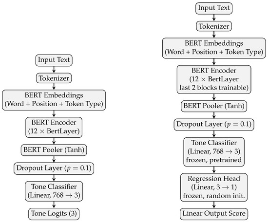
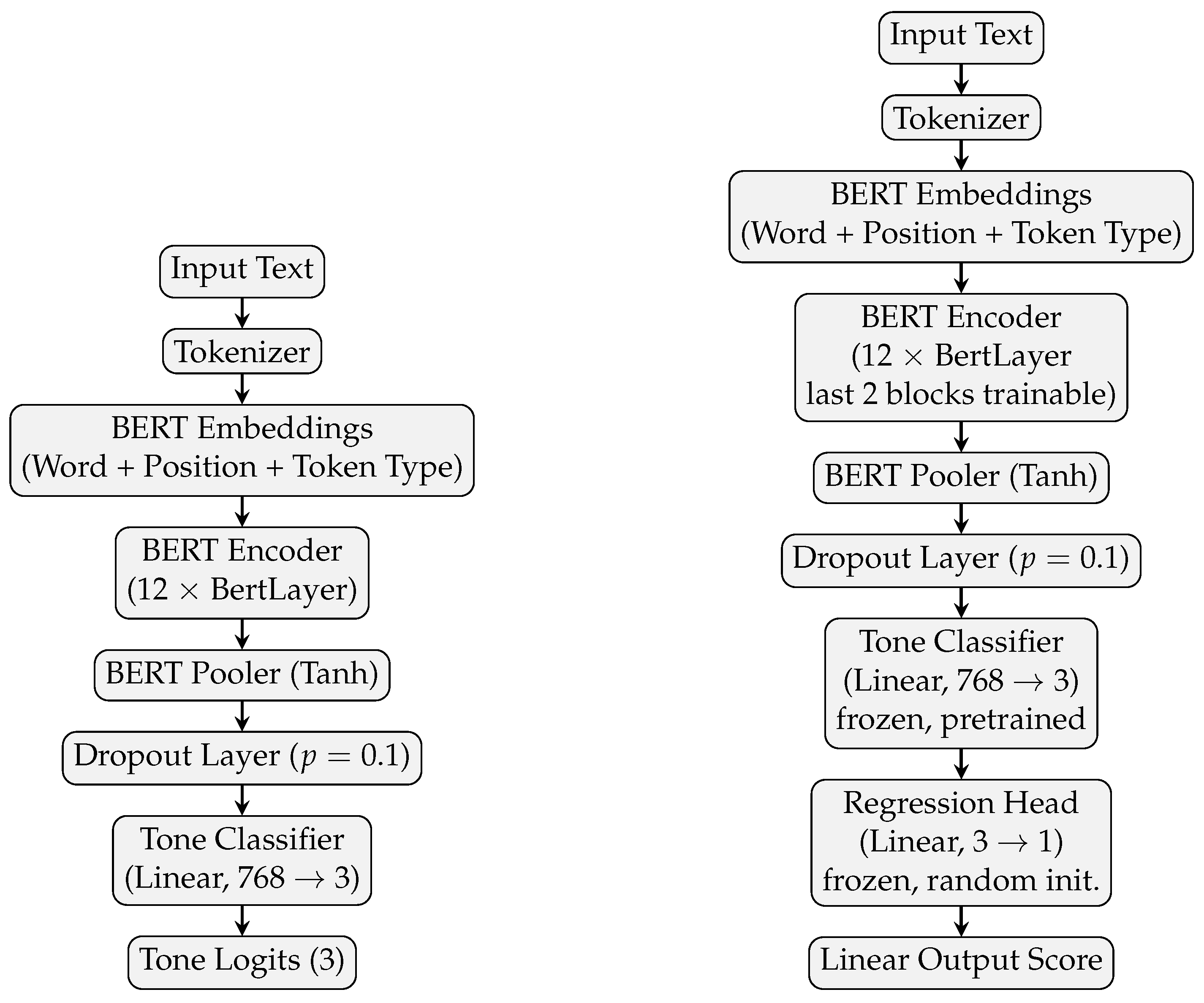
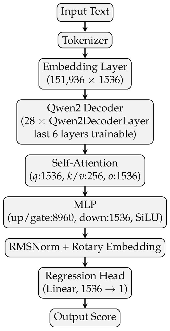
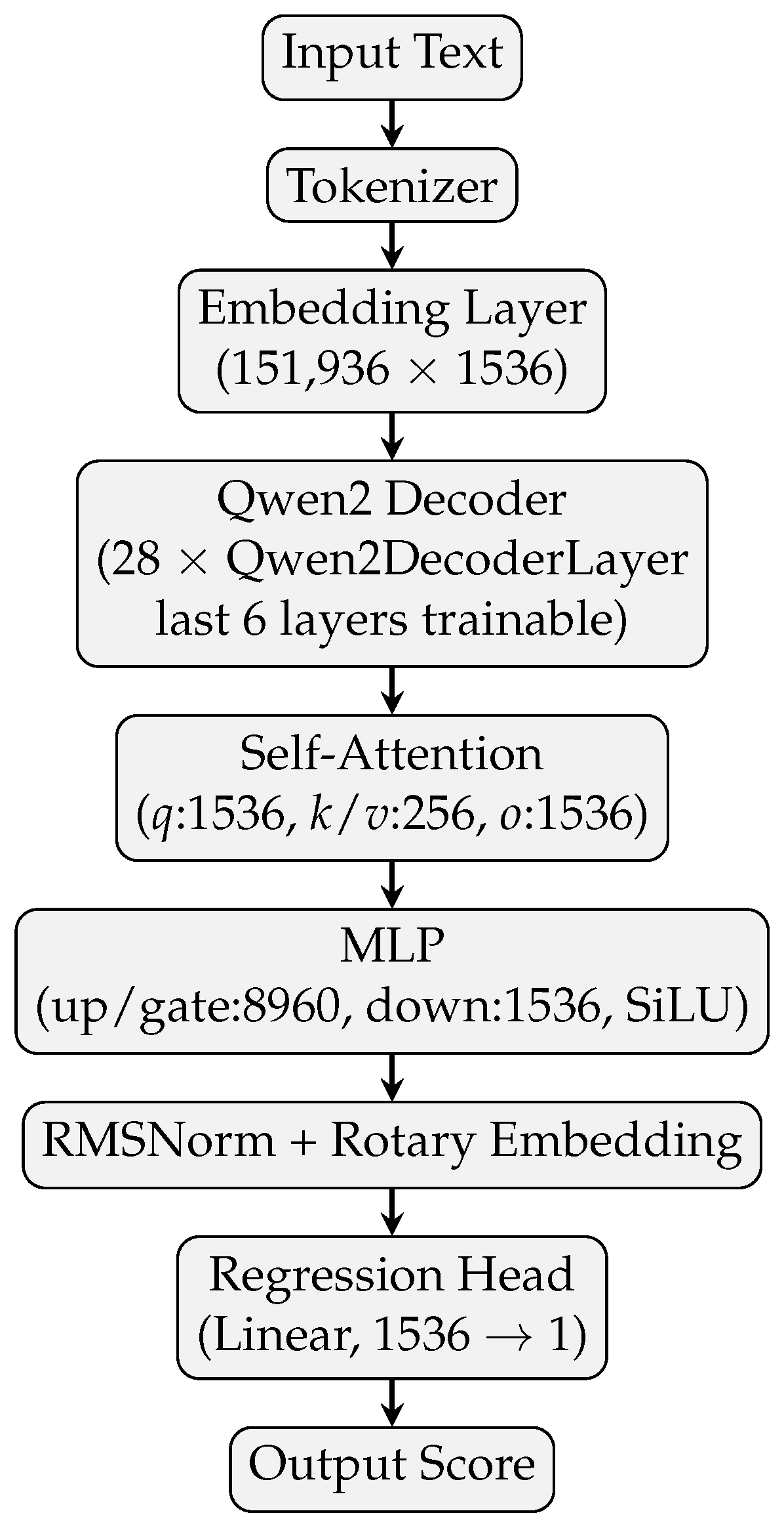
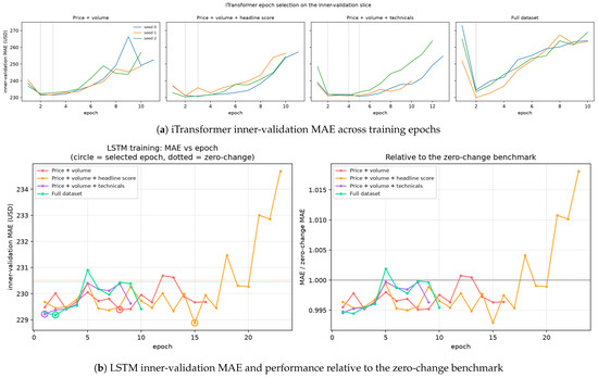
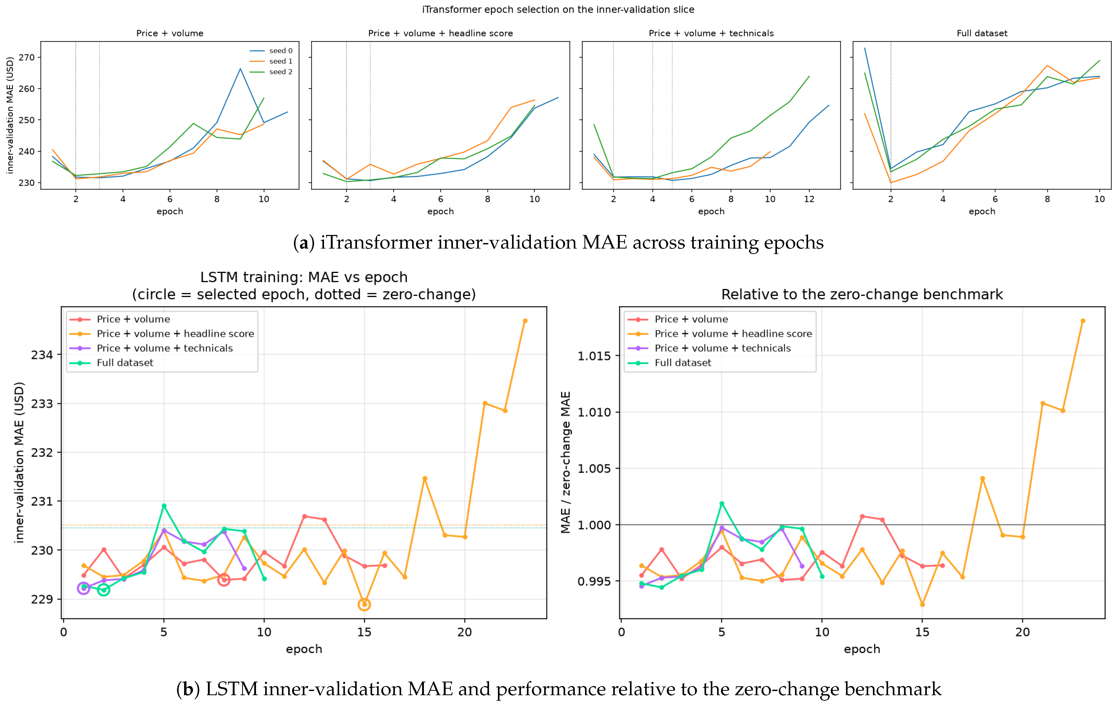
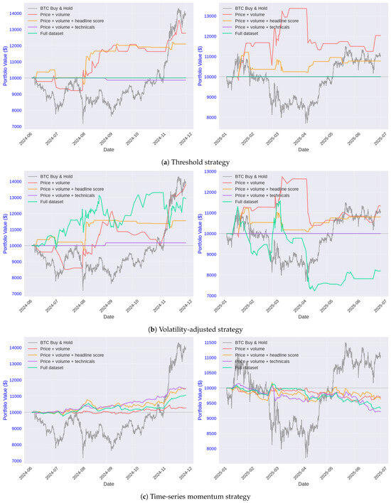
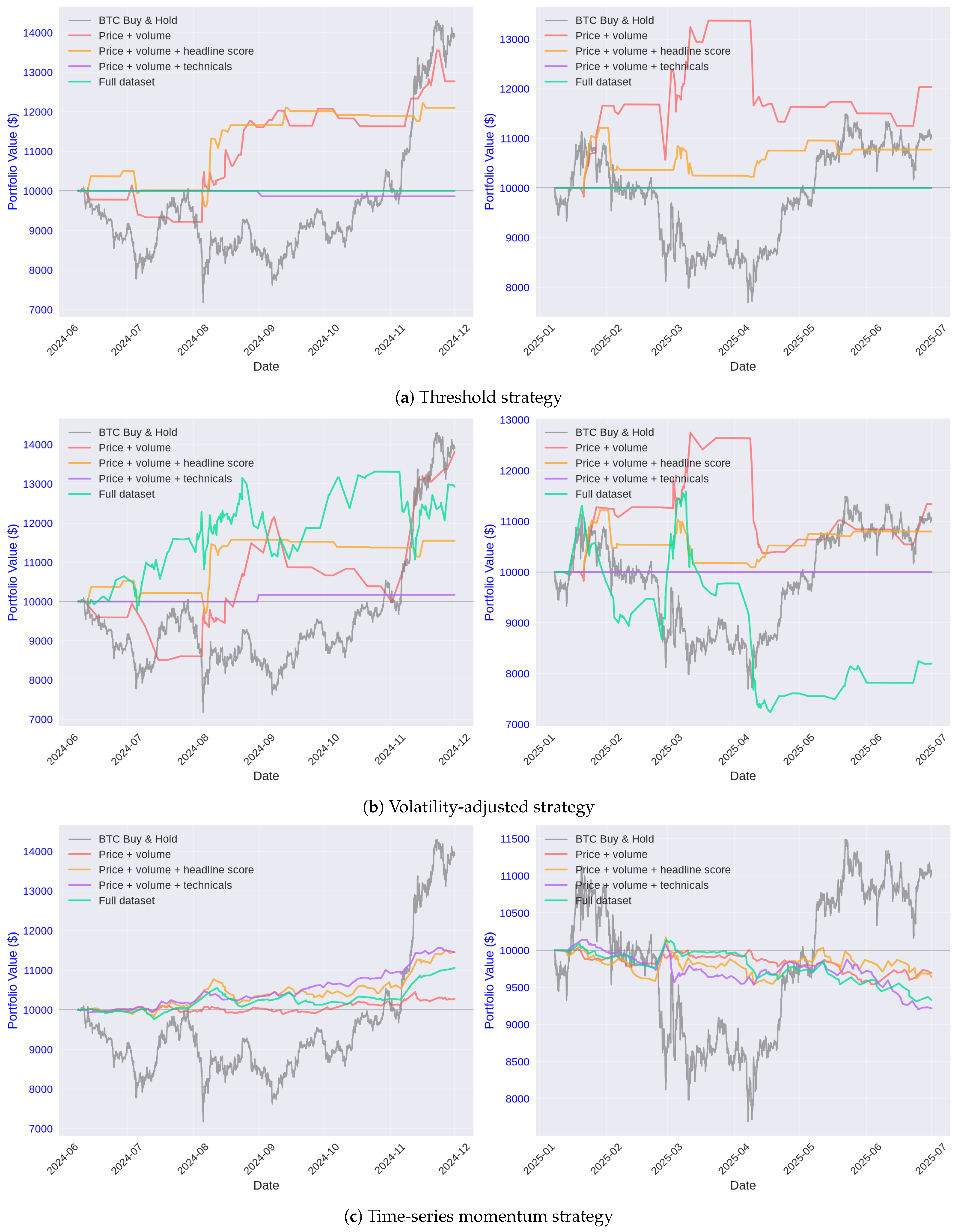
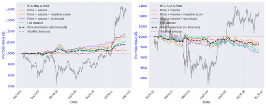
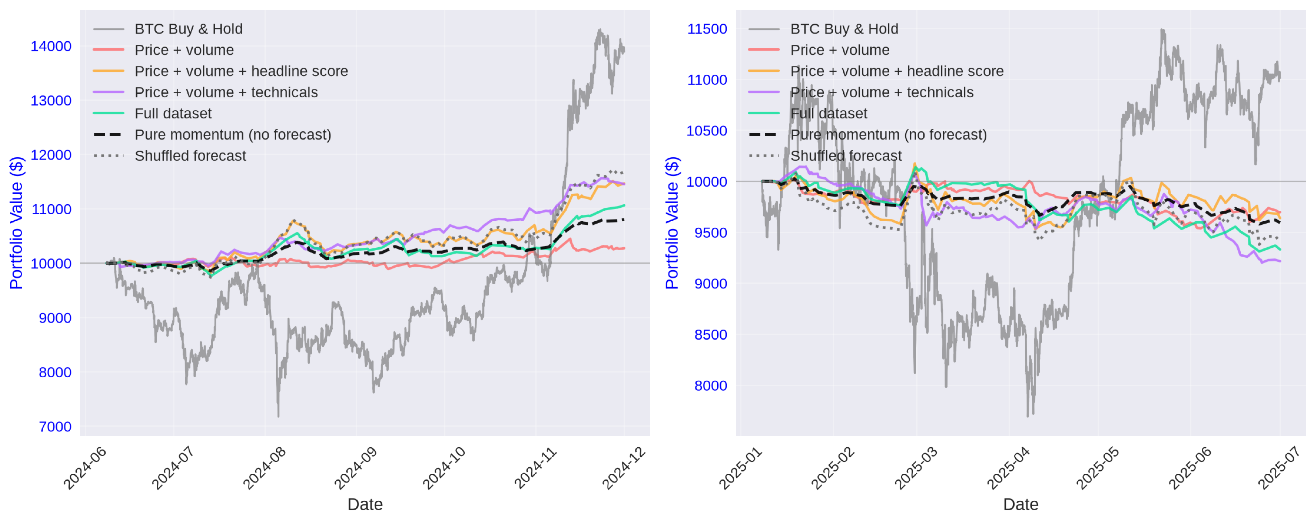

Disclaimer/Publisher’s Note: The statements, opinions and data contained in all publications are solely those of the individual author(s) and contributor(s) and not of MDPI and/or the editor(s). MDPI and/or the editor(s) disclaim responsibility for any injury to people or property resulting from any ideas, methods, instructions or products referred to in the content. |
© 2026 by the authors. Licensee MDPI, Basel, Switzerland. This article is an open access article distributed under the terms and conditions of the Creative Commons Attribution (CC BY) license.