Directional Inhibition Network (DI-Net): An Inspectable Retina-Inspired Code for Controlled GT-Isolated One-Pixel Eight-Way Direction Classification

Abstract

A long-standing account of retinal direction selectivity states that asymmetric inhibition suppresses responses to motion in the null direction. We use this idea as a computational prior in the Directional Inhibition Network (DI-Net), a two-stage model for direction classification from a before/after image pair. The first stage is a deterministic, parameter-free, anti-coincidence encoder that produces eight spatial maps of local directional evidence. The second is a compact convolutional network that combines this evidence into a global direction estimate. Because only the second stage is learned, the intermediate code remains directly inspectable. Experiments use object-conditioned pairs derived from DIS5K, with controlled translations and corruption applied only at test time. For one-pixel motion, DI-Net achieves 0.993 Accuracy on clean pairs and 0.747 under 10% corruption, close to Lucas–Kanade in the same evaluation. Fixed-channel voting reduces clean Accuracy to 0.713, whereas a convolutional network trained directly on the image pair degrades much more sharply under corruption. A multi-step version of the encoder also improves direction classification for displacements from 1 to 16 pixels compared with a parameter-matched one-step control. Tests on selected DAVIS-derived pairs show no statistically resolved difference between DI-Net and the evaluated optical-flow baselines. Taken together, these results support DI-Net as an interpretable, retina-inspired computational model for controlled motion-direction tasks rather than as a physiological account of retinal processing.

1. Introduction

Vision begins with retinal processing before signals reach downstream neural systems [1,2,3]. Specialized retinal circuits support efficient motion computation under constraints on energy, latency, and wiring [4,5,6,7]. This motivates using selected biological motifs as explicit algorithmic priors while evaluating the resulting systems on computational, rather than physiological, terms [8,9,10].

Retinal circuits derive direction selectivity from organized inhibitory interactions [7,11,12,13]. Classical inhibitory accounts and motion-energy models describe distinct mechanisms for direction-sensitive computation [14,15,16]. Recent retina-inspired systems span small-target motion, direction–speed detection, grayscale motion pathways, and neuromorphic motion processing [17,18,19,20]. Here these lines only motivate a discrete ordering rule; DI-Net does not reproduce retinal timing, anatomy, cell types, or circuitry.

Our earlier deterministic model combined a Barlow-inspired anti-coincidence encoder with fixed activation-count voting [21]. The present study asks whether a compact learned spatial integrator can use this inherited direction-indexed code on more complex object supports, whether multiple displacement steps extend the mechanism from minimal motion to longer-displacement direction discrimination, and whether the code itself has quantifiable spatial semantics. The task-aligned comparison with the predecessor is implemented as an encoder-only voting ablation and reported in Section 4.3; the multi-step extension is evaluated over 1–16 pixels in Section 4.4.

• Contributions

Our main contributions are as follows:

• We replace the inherited fixed activation-count readout with a compact learned spatial integrator and quantify the resulting gain using an encoder-only prior-work proxy under the same DIS5K-derived protocol.
• We extend the direction-indexed front end from a single displacement step to a dense 1–16-step bank and show, through equal-weight averages over all sixteen pixel displacements, that the multi-step mechanism supports longer-displacement eight-way direction discrimination.
• In the main experimental line, we benchmark DI-Net under the complete five-family DIS5K protocol against an adapted published TSM-MobileNetV2-2f reference and the MaskPair-CNN and PairLift-CNN representation controls. The three-row component ablation covers clean, 2.5%, 5%, 7.5%, and 10% corruption.
• Supplementary analyses quantify direction-indexed localization on all 2470 held-out pairs and report family- and training-run-specific behavior, paired TSM and five-seed MaskPair analyses, three deterministic transformations, and a selected DAVIS-derived multi-gap task under explicitly separated protocols.

2. Related Work

2.1. Bio-Inspired and Circuit-Motivated Vision

Comparing bio-inspired systems requires separating the native task, sensory input, output, explicit mechanism, and learning locus. Representative systems embed orientation selectivity, cortical front ends, or excitation–inhibition motifs into learned networks [22,23,24,25,26]. Motion-oriented neighbors include retinal small-target and direction–speed systems and data-driven models of human motion processing [17,18,19,27]. Their tasks and intermediate representations differ from DI-Net.

Learning-based motion-direction systems include a dendritic artificial visual system [28] and a horizontal-cell-based dendritic model [29]. Qiu et al. [30] retained a local motion detector and used Gaussian-mixture-model-based unsupervised grouping for global direction detection. In contrast, the primary DI-Net model retains a fixed anti-coincidence encoder and trains a supervised CNN to integrate its spatial evidence maps.

Most directly related is our earlier deterministic model [21], which combined Barlow-inspired local anti-coincidence units with fixed activation-count voting on successive $32\times 32$ synthetic binary patterns. Because the original publication used a different dataset and execution protocol, its published scores are not compared directly with the present results. Instead, the encoder-only voting variant in Section 4.3 retains the inherited deterministic encoder and reinstates the defining fixed channel-count readout within the current DIS5K-derived protocol. It therefore serves both as a component ablation and as the task-aligned quantitative proxy for the most directly related bio-inspired predecessor. The proxy obtains 0.713 Accuracy and 0.685 Macro-F1 scores, compared with 0.993/0.993 for DI-Net, identifying learned spatial evidence integration as the principal functional extension. The broader bio-inspired methods in Table 1 remain conceptual comparators because their tasks, sensors, and native outputs are not commensurate with this eight-way direction-classification protocol.

Table 1. Structured positioning of DI-Net relative to representative mechanistic, bio-inspired, neuromorphic, structured-compensation, and motion-estimation lines. Native tasks, inputs, outputs, and supervision differ; the table is a conceptual comparison, not a cross-task performance ranking.

Work or Family	Native Task/Output	Input	Explicit Mechanism and Learning Locus	Relation to DI-Net
Earlier Barlow-inspired detector [21]	Discrete motion direction	Two successive synthetic binary pattern images	Fixed anti-coincidence units and activation-count vote; no learned spatial integrator	Direct antecedent; the encoder family is inherited
Orientation-selective visual systems [22,23]	Image orientation	Grayscale or RGB image	Explicit selectivity motifs; learning role depends on the system	Related selectivity mechanisms, but not paired-frame motion
Hubel–Wiesel and dendritic systems [25,26]	Object detection or classification	Task-specific images or features	Cortical or dendritic excitation–inhibition motifs embedded in learned task networks	Mechanistic-learning context with different tasks and intermediate semantics
Event/neuromorphic vision [31,32]	Motion, flow, or recognition	Asynchronous events or spikes	Event/spike encoding and temporal processing; estimator-dependent learning	Different sensor and temporal representations; DI-Net is frame-based and non-spiking
Retina-inspired motion systems [17,18,19]	Small-target, direction, or direction–speed output	Grayscale/RGB scenes or engineered pathways	Explicit retinal/cortical motifs with task-specific learning	Direct thematic neighbors with non-identical inputs and protocols
Temporal Shift Module [33]	Video recognition; here adapted to eight-way direction	Multi-frame RGB; here two ordered frames	Parameter-free temporal channel shifts inside a learned 2D backbone	Published temporal reference, but the $T=2$ adaptation is not representation- or capacity-matched
Optical-flow estimation [34,35,36,37,38]	Sparse or dense displacement field	Two intensity frames	Optimization, polynomial expansion, cost volumes, or learned correlation/refinement	Native output differs; flow is quantized only as a task reference
STSc-GCN [39]	Skeleton-based action recognition	Multi-frame human-joint skeleton sequence	Learned CMSC joint-topology compensation and MSTC cross-attention temporal sharpening	Broader data-compensation context; no fixed directional inhibitory code
DI-Net (this work)	Object-conditioned eight-way direction	Before/after RGB converted to binary receptor maps	Inherited fixed eight-hypothesis anti-coincidence code; only the CNN integrator is learned	Learned integration plus direct analysis of code semantics and failure boundaries

A second within-study test extends the inherited one-step regime to direction discrimination at larger displacements. In the separate $q=1,\dots ,16$ experiment, the dense 16-step front end averages 0.995/0.995 clean and 0.991/0.991 under the fixed 10% corruption, whereas the parameter-matched one-step control averages 0.777/0.777 and 0.690/0.688. These equal-weight results show that the multi-step directional code remains effective across all sixteen evaluated pixel displacements. Table 2 summarizes the structural differences between the earlier deterministic study and DI-Net.

Table 2. Direct structural comparison between the earlier deterministic study and DI-Net. The studies use different data, preprocessing, and execution protocols; no cross-publication performance ranking is implied.

Dimension	Earlier Deterministic Study [21]	DI-Net (Present Study)
Encoding rule	Barlow-inspired local direction-selective inhibitory/veto units applied to two successive binary pattern images	The inherited eight-direction veto family formalized as a fixed, foreground-area-normalized anti-coincidence evidence tensor; the encoder is not claimed to be new
Readout mechanism	Count local-unit activations for each direction and use an argmax decision to select the global direction	Use a learned three-block CNN to integrate the eight-channel spatial evidence tensor, followed by global average pooling and an eight-class head
Learning location	There is no learned spatial integrator in the proposed deterministic detector; the CNN in the earlier study was evaluated separately as a comparator	Decoder only; the encoder remains fixed and parameter-free
Experimental task and evaluation scope	Infer one of eight global motion directions from two successive $32\times 32$ synthetic binary light-spot or random-dot pattern images, including tests with added noise	Classify GT-derived, object-conditioned before/after pairs in the one-pixel primary protocol and a controlled 1–16-pixel multi-step extension
New contribution	A deterministic local-to-global motion-direction mechanism combining Barlow-inspired local units with fixed activation-count aggregation	Learned spatial integration of the inherited direction-indexed code, plus multi-step longer-displacement direction discrimination and controlled representation-level analysis

2.2. Motion and Displacement Estimation

Recovering displacement from an image pair is a classical problem. Classical optical flow includes global smoothness [34], local least squares [35], and polynomial expansion [36]. Learned estimators include pyramid/warping designs and all-pairs iterative refinement [37,38]; event-based methods instead exploit an asynchronous temporal structure [32,40]. These estimator families provide conceptual context rather than a task-matched benchmark in the present study. These estimators recover motion effectively, but they return a displacement or a dense flow field without explicit, per-hypothesis mechanistic semantics that can be inspected channel by channel. Our objective is complementary: rather than maximizing raw estimation accuracy, we evaluate an explicit inhibitory evidence code in the primary minimal-displacement regime and then extend its direction hypotheses to 1–16 pixel steps for longer-displacement direction discrimination.

As a published learned temporal reference, the Temporal Shift Module (TSM) inserts parameter-free channel shifts into a two-dimensional backbone for video understanding [33]. We adapt the TSM with a MobileNetV2 backbone to two ordered frames and eight direction logits. Because the original work primarily considered longer clips, our $T=2$ configuration is a task-specific adaptation trained from scratch, not a reproduction of a published result on this direction task.

Two author-constructed controls address representation questions that the external TSM comparison cannot isolate. MaskPair-CNN learns directly from the same two receptor maps with near-matched capacity and an equal training budget. PairLift-CNN v6 first applies a learned bias-free $1\times 1$ two-to-eight-channel lift and then uses the unchanged DI-Net decoder; the reported result uses one training seed and a post hoc epoch-6 checkpoint selected using clean-training information only. The TSM is external and published but differs in input representation and capacity. Together, these methods provide complementary internal representation controls and an external temporal reference, not three strictly matched external comparators.

A complementary route to robustness under constrained observations is learned spatial–temporal self-compensation. Li et al.’s STSc-GCN targets skeleton-based action recognition when skeleton sequences are degraded by body occlusion, missing frames, or noise [39]. Its collaborative motion spatial compensation (CMSC) module models universal and personalized relationships among human joints to compensate for spatial information loss, while its meta-action sharpening temporal compensation (MSTC) module uses cross-attention-based motion sharpening under missing-frame conditions. STSc-GCN is a learned compensation architecture operating on multi-frame skeleton graphs, whereas DI-Net neither reconstructs missing joints or frames nor learns a compensation graph. DI-Net’s fixed encoder instead maps one object-conditioned binary before/after pair into eight directional anti-coincidence channels, and only the downstream CNN learns their spatial integration. We therefore cite STSc-GCN as complementary context, not as a task-matched baseline or evidence of universal robustness for DI-Net.

Recent cross-modal studies provide a second form of conceptual context. Band-Mixed combines edge-aware supervision with RGB–thermal interaction for camouflaged-object detection [41], whereas Co-D² uses radar-derived structural cues for infrared detection and de-ghosting [42]. Their modalities, tasks, outputs, datasets, and metrics differ from DI-Net’s object-conditioned paired-frame classification; they are therefore related examples of structured cue integration, not task-matched numerical baselines or validation of the anti-coincidence mechanism.

2.3. Interpretable and Mechanistic Deep Learning

Mechanistic and interpretable learning emphasizes explicit internal structure and testable intermediate representations rather than post hoc explanation alone [10,24,27,43]. DI-Net evaluates interpretability at the representation level through component ablation and spatial localization of the direction-indexed pre-decoder code. These analyses test where task-relevant evidence is expressed, while remaining distinct from decoder-causality claims, post hoc attribution, human interpretability studies, or physiological validation.

3. Mechanism and System

This section formalizes the implemented anti-coincidence operator and the CNN evidence integrator. Biological terminology is used only to motivate the ordering relation defined below.

3.1. Biological Inspiration: An Asymmetric-Inhibition Motif

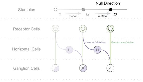
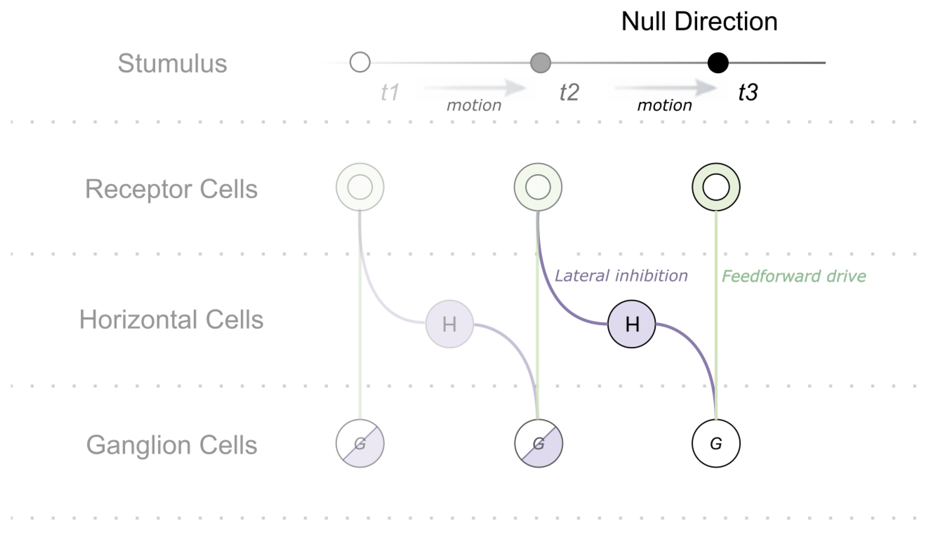
The classical Barlow–Levick account attributes direction selectivity to temporally asymmetric suppression of null-direction motion [14,15,44]. Figure 1 illustrates the biological motif that inspired DI-Net: a moving stimulus successively engages spatially offset receptors, while a lateral pathway can oppose feedforward drive at the readout. The drawing supplies a conceptual drive-and-veto relation only; it is not a circuit diagram of the implemented model.

Figure 1. Asymmetric lateral-inhibition motif motivating DI-Net. (Top): A schematic null-direction stimulus progresses across three spatial positions ($t_1$–$t_3$). (Bottom): The source biological abstraction contrasts receptor-driven feedforward drive with a laterally mediated inhibitory pathway converging on a ganglion-cell readout. The receptor, horizontal-cell, and ganglion-cell labels describe the motivating retinal account only. DI-Net does not instantiate these cell types or simulate temporal delays, membrane or synaptic dynamics, spiking, adaptation, or complete retinal circuitry.

From this schematic, DI-Net only retains the computational asymmetry: drive-like evidence is admitted when the opposed evidence is absent. The implementation replaces named retinal pathways and temporal-delay dynamics with deterministic spatial tests on two ordered binary receptor maps. Accordingly, before/after order is an input convention, not a simulated synaptic delay, and the learned CNN is an engineering evidence integrator rather than a ganglion-cell model.

3.2. Algorithmic Instantiation of the Discrete Anti-Coincidence Rule

The implementation is a two-lobed spatial anti-coincidence operator. At an active after-map site, it samples opposed locations in the before map for each candidate displacement and emits support only when the driving sample is present and the opposing sample is absent.

The candidate displacement axes are the first-order lattice-neighborhood displacement set,

$${\mathcal{N}}_1=\{d=(\Delta y,\Delta x)\in {\mathbb{Z}}^2:{\parallel d\parallel }_{\infty }{=1\}=\{-1,0,1\}}^2\setminus \left\{(0,0)\right\}.$$

This center-excluded Chebyshev radius-one neighborhood is the eight-connected Moore neighborhood of a two-dimensional image lattice, whose elements we order as

$${\mathcal{N}}_1=\{d^{\left(1\right)},\dots ,d^{\left(M\right)}\},M=\left|{\mathcal{N}}_1\right|.$$

In the present two-dimensional setting, $M=8$. Accordingly, the shorthand labels in the figures (“Eight-Dir Encoder” and “8-Direction Inhibition”) and the schematic notation ${\mathbb{R}}^{8\times H\times W}$ all denote this $M=|{\mathcal{N}}_1|=8$ instantiation, not an arbitrary eight-class motion convention. The accompanying angle labels are merely a convention for ordering the elements of ${\mathcal{N}}_1$; we state this once here and do not repeat it in the individual figure captions.

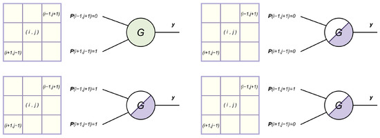
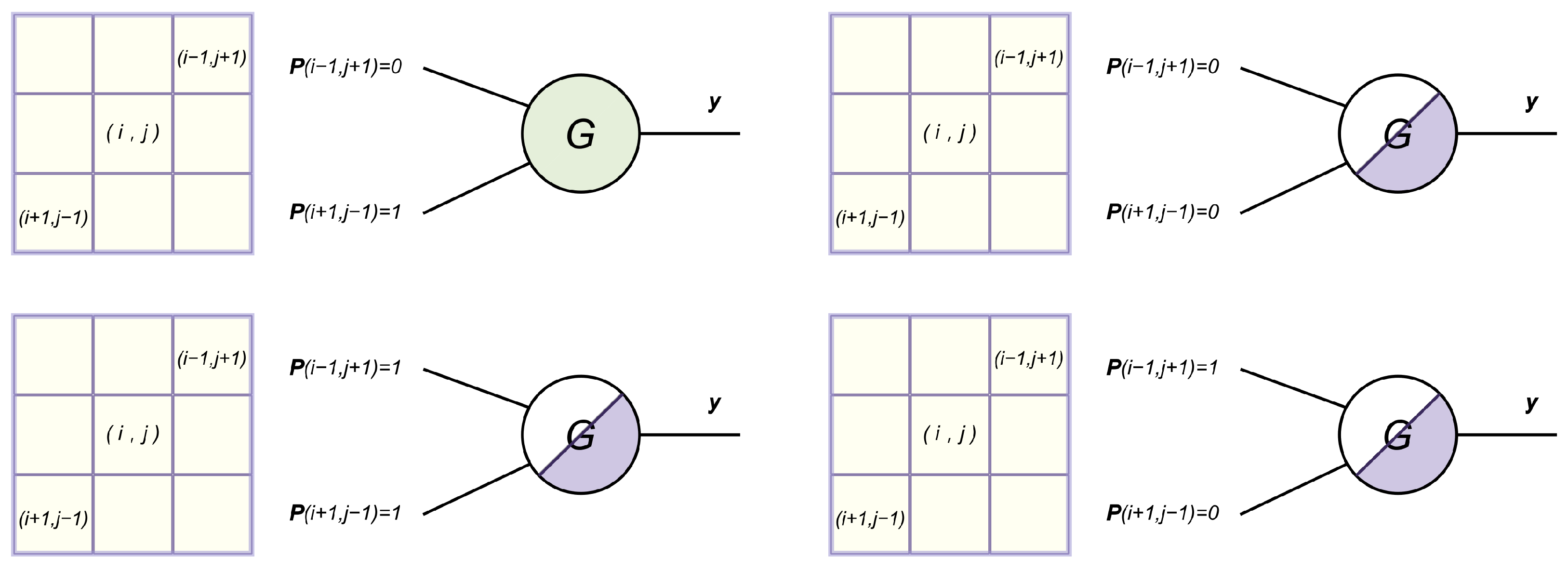
For one representative axis, Figure 2 enumerates the four binary input configurations. Tiling the same rule across space and over every hypothesis in ${\mathcal{N}}_1$ yields the neighborhood-indexed evidence tensor. Figure 3 illustrates the deterministic encoder.

Figure 2. Implemented two-lobed anti-coincidence operator. The operator compares opposed samples for each displacement hypothesis and emits support only when the driving sample is active and the opposing sample is inactive. Here G denotes an abstract Boolean gate. Green denotes an active gate, whereas purple-shaded crossed gates denote inactive outputs.

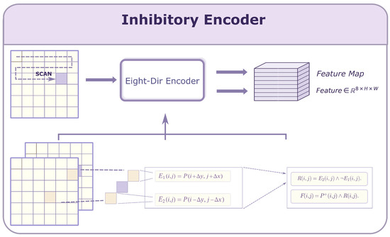
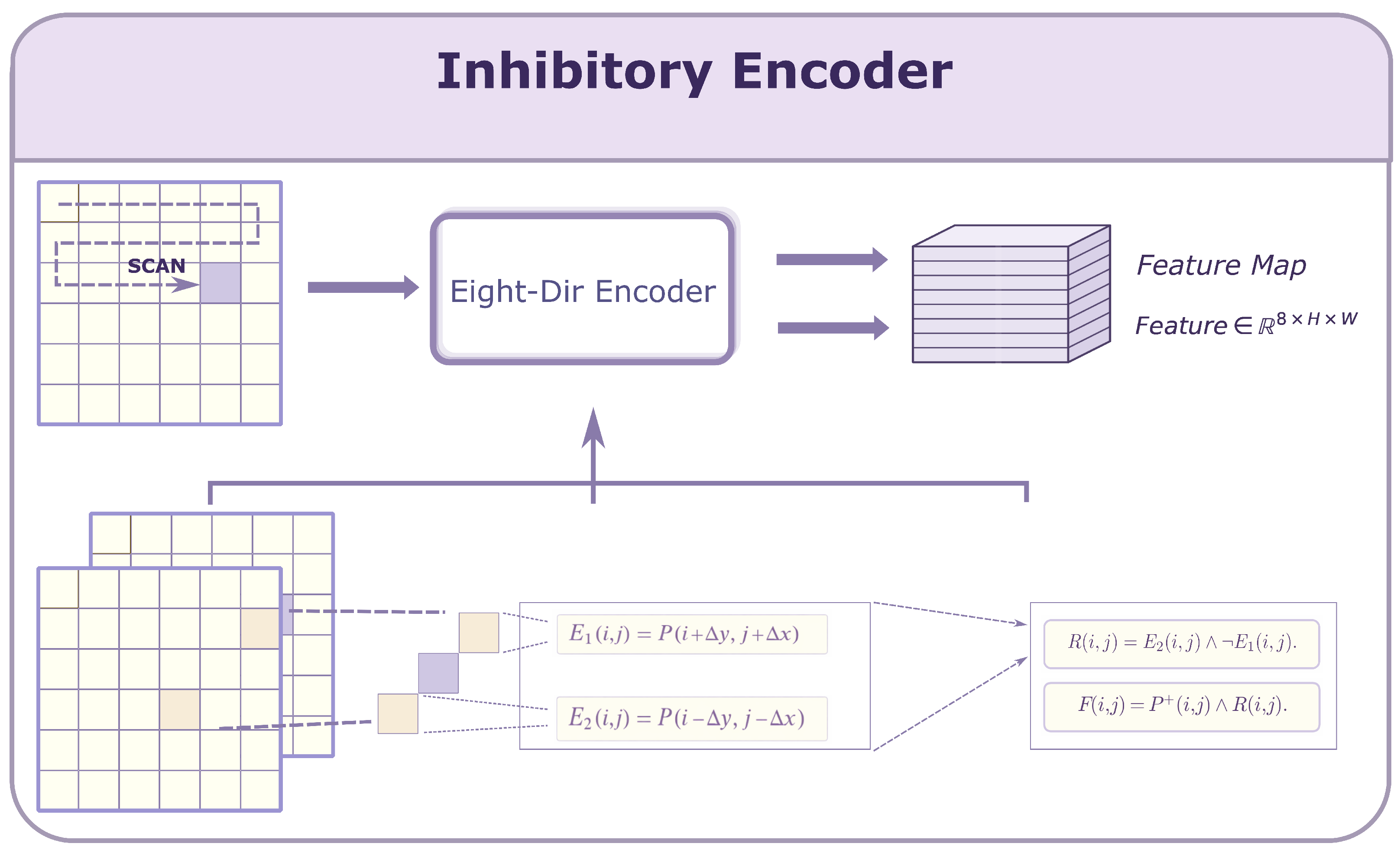
Figure 3. Implemented deterministic anti-coincidence encoder. At each active after-map site, opposed before-map samples are evaluated for the eight displacement hypotheses. The binary support tensor is normalized by the active after-map area before it is passed to the CNN. Arrows indicate the flow of sampling and encoding operations; colors distinguish schematic components.

3.3. Implemented Anti-Coincidence Encoder

Let $P,P^{+}\in {\{0,1\}}^{H\times W}$ denote the RGB-derived binary support maps for the before and after observations, with zero extension outside the image lattice $\mathsf{\Omega }$. We retain the shorthand receptor maps for implementation consistency; these arrays are thresholded image supports, not modeled photoreceptor responses. Channels follow the ordered set ${\mathcal{N}}_1=\{d^{\left(1\right)},\dots ,d^{\left(M\right)}\}$, where $M=8$. For a candidate applied displacement $d^{\left(k\right)}$ and an active after site x, the implementation samples

$$D^{\left(k\right)}\left(x\right)=P\left(x-d^{\left(k\right)}\right),I^{\left(k\right)}\left(x\right)=P\left(x+d^{\left(k\right)}\right).$$

(1)

The binary anti-coincidence support is

$${\tilde{F}}^{\left(k\right)}\left(x\right)=P^{+}\left(x\right)\wedge D^{\left(k\right)}\left(x\right)\wedge \neg I^{\left(k\right)}\left(x\right).$$

(2)

The implementation normalizes by the active after-map area,

$$N^{+}=\sum _{x\in \mathsf{\Omega }}{P}^{+}\left(x\right),$$

(3)

$$F^{\left(k\right)}\left(x\right)=\left\{\begin{array}{cc}{\tilde{F}}^{\left(k\right)}\left(x\right)/(N^{+}+{10}^{-6}),\hfill & N^{+}>0,\hfill \\ 0,\hfill & N^{+}=0,\hfill \end{array}\right.\mathbf{F}={\mathrm{stack}}_{k=1}^M{F}^{\left(k\right)}\in {\mathbb{R}}_{\ge 0}^{M\times H\times W}.$$

(4)

The support tensor $\tilde{\mathbf{F}}$ is binary, whereas $\mathbf{F}$, which is passed to the CNN, is real valued. It is an explicit direction-indexed representation, not a dense optical-flow field or a modeled neural response.

3.4. CNN Decoder for Hierarchical Evidence Integration

The encoder hands the decoder an explicit neighborhood-indexed evidence tensor $\mathbf{F}\in {\mathbb{R}}_{\ge 0}^{M\times H\times W}$ (Equation (4)), formed by stacking ${\left\{F^{\left(k\right)}\right\}}_{k=1}^M$ in the fixed order of ${\mathcal{N}}_1$ (Section 3.3). The decoder ${\varphi }_{\theta }$ integrates these sparse, spatially scattered events into a global displacement-direction decision while remaining agnostic to the absolute position.

• Convolutional integration

Three $3\times 3$ convolutional blocks with zero-padding preserve the $H\times W$ lattice. With ${\mathbf{F}}^{\left(0\right)}=\mathbf{F}$ and ${\mathbf{F}}^{(\ell )}$, the feature map after block ℓ, for $\ell \in \{1,2,3\}$,

$${\mathbf{F}}^{(\ell )}=\sigma \left({\mathrm{GN}}_g\left({\mathbf{K}}^{(\ell )}\ast {\mathbf{F}}^{(\ell -1)}\right)\right),$$

(5)

where ∗ is convolution, ${\mathbf{K}}^{(\ell )}$ the learnable kernel bank of block ℓ, ${\mathrm{GN}}_g(·)$ Group Normalization with g groups, and $\sigma (·)$ ReLU. Channel widths follow $M\to 32\to 64\to 64$ ($M=8$ here), so ${\mathbf{F}}^{\left(3\right)}\in {\mathbb{R}}^{64\times H\times W}$ encodes higher-order spatial conjunctions of the original neighborhood-indexed evidence.

• Global pooling and readout

A global average pooling (GAP) over $\mathsf{\Omega }$ produces a position-invariant summary,

$$\mathbf{h}=\mathrm{GAP}\left({\mathbf{F}}^{\left(3\right)}\right)\in {\mathbb{R}}^{64},h_c={\displaystyle \frac{1}{HW}}\sum _{(i,j)\in \mathsf{\Omega }}{F}_{c,i,j}^{\left(3\right)},$$

(6)

with $c\in \{1,\dots ,64\}$ indexing channels, and a dropout-regularized two-layer linear head maps $\mathbf{h}$ to logits $\mathbf{s}\in {\mathbb{R}}^M$:

$$\mathbf{s}={\mathbf{U}}_2\sigma \left({\mathbf{U}}_1\mathrm{Dropout}\left(\mathbf{h}\right)\right),s_c\mathrm{is}\mathrm{the}c-\mathrm{th}\mathrm{logit},$$

(7)

where ${\mathbf{U}}_1$ and ${\mathbf{U}}_2$ are learnable weight matrices. The softmax posterior is

$$p_{\theta }(y\mid \mathbf{F})={\displaystyle \frac{\exp \left(s_y\right)}{{\sum }_{c=1}^M\exp \left(s_c\right)}},y\in \{1,\dots ,M\}.$$

(8)

This yields the direction scores ${\varphi }_{\theta }\left(\mathbf{F}\right)=\mathbf{s}$ and the predicted class $\widehat{y}=\arg {\max }_c{s}_c$.

• Training objective and modularity

For a labeled sample $(\mathbf{F},y)$, all decoder parameters are trained with multi-class cross-entropy:

$$\mathcal{L}\left(\theta \right)=-\log p_{\theta }\left(y|\mathbf{F}\right).$$

(9)

Because the anti-coincidence encoder (Section 3.3) is deterministic and parameter-free, all trainable parameters reside in the CNN, which learns to integrate the fixed logical evidence.

• Encoder complexity.

For M direction hypotheses on an $H\times W$ lattice, evidence construction requires $O\left(MHW\right)$ time and $O\left(MHW\right)$ output storage. A radius bank S requires $O\left(\right|S\left|MHW\right)$ evidence-construction work. Parameter-free therefore does not mean computation-free, and these bounds exclude the learned decoder.

3.5. System Architecture

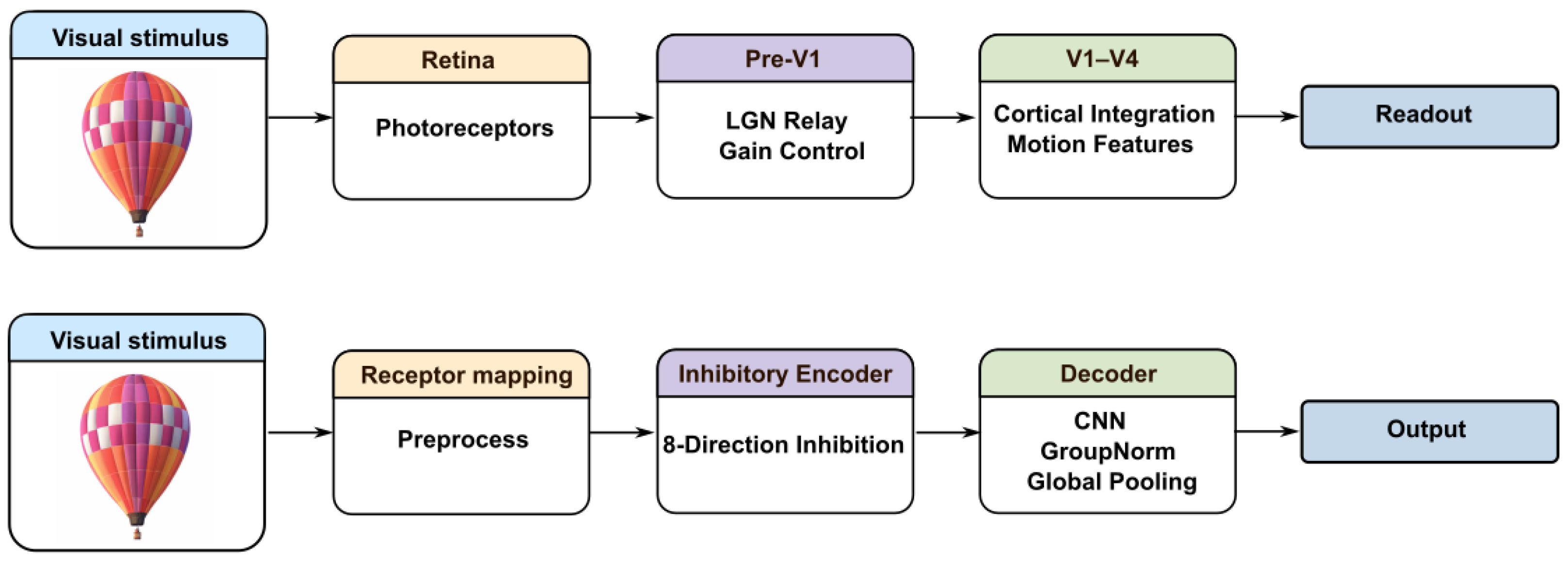
Figure 4 summarizes the implemented mapping. Given $(P,P^{+})$, the fixed encoder produces the direction-indexed tensor $\mathbf{F}$ defined in Equation (4), and the decoder in Section 3.4 maps $\mathbf{F}$ to eight direction logits:

$$(P,P^{+})⟼\mathbf{F}\stackrel{{\varphi }_{\theta }}{\to }\mathbf{s}\in {\mathbb{R}}^M\stackrel{\mathrm{softmax}}{\to }{p}_{\theta }(y\mid \mathbf{F}),\widehat{y}=\arg \underset{c\in \{1,\dots ,M\}}{\max }{s}_c.$$

(10)

This modular mapping supports the encoder-only and raw-pair component ablations defined in Section 4.1.

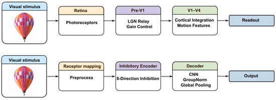
Figure 4. Implemented two-stage algorithmic pipeline. The first stage is a fixed logical operator and the second is a learned spatial integrator.

4. Experiments

4.1. Experimental Setup

• Dataset split and preprocessing

We retain the official DIS5K roles without re-splitting: all 3000 DIS-TR images are used for training, and DIS-VD together with DIS-TE1–4 provides 2470 non-TR evaluation images [45]. For each source, the GT map is thresholded above zero and RGB outside that support is set to zero. The full masked frame is not bounding-box-cropped. It is downscaled only when a spatial dimension exceeds 256, using nearest-neighbor interpolation with preserved aspect ratio, and centered on a zero-valued transparent $256\times 256$ RGBA canvas; smaller frames are not enlarged. The encoder ignores alpha and forms the RGB-derived receptor map

$$P\left(x\right)=⊮\left[\underset{c\in \{R,G,B\}}{\max }{I}_c\left(x\right)>0\right].$$

(11)

Thus, GT supplies object isolation, while the encoder consumes RGB-derived support. Alpha is retained for cohort construction and localization targets but is not passed to the encoder. The binary direction-indexed support is normalized by the active after-frame receptor count plus ${10}^{-6}$; cached evidence is stored as float16 and loaded as float32. DI-Net applies no ImageNet normalization.

• Pair construction under minimal first-order lattice displacement

In the $(\Delta y,\Delta x)$ coordinates, the ordered displacement set is

$${\mathcal{N}}_1=[(0,1),(1,1),(1,0),(1,-1),(0,-1),(-1,-1),(-1,0),(-1,1)].$$

(12)

A NumPy RandomState with motion seed 12345 selects one displacement per source. The complete RGBA array is translated once with zero filling, and its index is the class label for every method. Diagonal motion is one Chebyshev-lattice step. This fixed offline pair construction is not online augmentation. No learned segmentation model, predicted mask, original full-scene input, or segmentation-free deployment pipeline is evaluated.

• Primary and supplementary experiments

The main experimental line contains three result blocks: the eleven-method one-pixel DIS5K comparison, the component ablation across clean and four corruption levels, and the separately trained controlled $q=1,\dots ,16$ multi-step experiment summarized by its equal-weight average. Appendix A.1 reports the family-resolved decomposition, localization analysis, salt-and-pepper comparator ladder, paired TSM and five-seed MaskPair studies, fixed-realization Gaussian-blur/reciprocal-exposure/label-preserving-rotation tests, and the separately trained selected DAVIS-derived multi-gap task. Metrics are never pooled across these distinct supplementary protocols. Table 3 summarizes the impulse-corruption parameters.

Table 3. Impulse-corruption parameterization. Sampling is separate for the two RGB frames over the complete $256\times 256$ lattice; p is an overwrite budget, not a guaranteed receptor-flip fraction.

Family	Spatial Draws per Frame	Sampling	Assignment
Salt-and-pepper	$\mathrm{round}\left(pHW\right)$ coordinates	Without replacement	Black/white, equiprobable
Salt-only	$\mathrm{round}\left(pHW\right)$ coordinates	Without replacement	White
Pepper-only	$\mathrm{round}\left(pHW\right)$ coordinates	Without replacement	Black
Random RGB	$\mathrm{round}\left(pHW\right)$ coordinates	Without replacement	Channels uniform on $\{0,\dots ,255\}$
Block impulse	$\max \{1,\mathrm{round}(pHW/25\left)\right\}$ blocks	Valid origins with replacement	$5\times 5$ black/white; later write wins

• Noise protocol

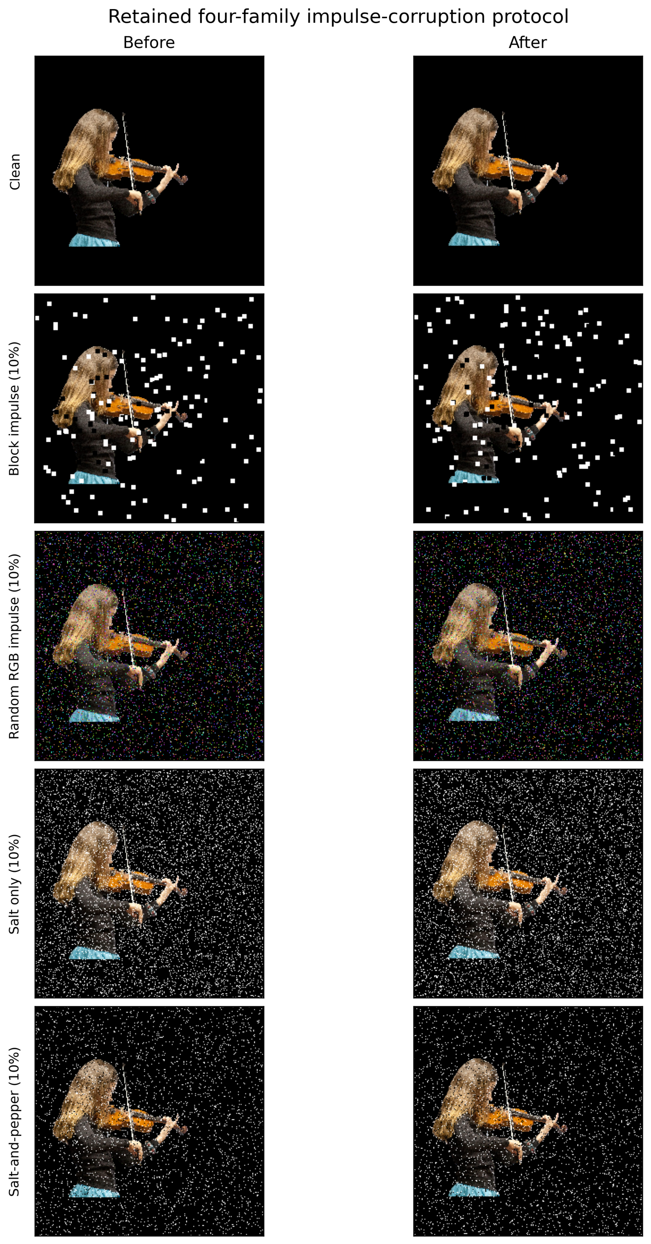
Corruption is applied after clean pair construction to the before and after RGB frames using distinct deterministic frame-role keys. At levels 2.5/5/7.5/10%, point families sample 1638/3277/4915/6554 coordinates uniformly without replacement; the $5\times 5$ block impulse samples 66/131/197/262 origins uniformly with replacement, permits overlap, and applies later-write overwrite. The complete main panel uses five families: block impulse, random RGB impulse, salt-only, pepper-only, and salt-and-pepper. Ten corruption-realization IDs (20260618–20260627) are used with fixed clean-trained checkpoints and no corruption-specific retraining. Appendix A.2 gives the complete keyed protocol; Figure A1 illustrates four representative families, with pepper-only following the same point-sampling rule and assigning black.

• Corruption and inference order

The clean cutout is centered, the translated after frame and label are fixed, and the two RGB frames are then corrupted separately. DI-Net subsequently thresholds RGB by the any-channel-positive rule, forms and normalizes the eight anti-coincidence channels, and invokes the CNN. Every method receives the same corrupted RGB pair before its own disclosed preprocessing.

• Metrics and statistical units

We report Accuracy and fixed-eight-class Macro-F1. Corruption-realization intervals resample ten realization summaries within one fixed checkpoint/family/level. Training-run summaries first average those ten realizations within each checkpoint and then summarize five independently trained checkpoints. These units are not pooled or interchanged; Appendix A.4 gives the run-level records and interval definitions.

Localization intervals use 20,000 complete-stem bootstrap replicates. This interval is conditional on the frozen checkpoint and does not cover training-run, target-definition, dataset, or deployment uncertainty.

• Compared methods

The primary representation control is MaskPair-CNN, which matches DI-Net in the receptor source, resolution, backbone/head family, data, seeds, and update budget, and near-matches its capacity, while replacing the eight-channel directional code with the two receptor maps. PairLift-CNN v6 is a second author-constructed representation control that learns a two-to-eight-channel pointwise lift before the unchanged decoder. The protocol-aligned deterministic readout inherited from our 2021 predecessor tests the non-neural stage alone; CNN-from-pair is a historical raw-pair ablation; TSM-MobileNetV2-2f is an external temporal reference aligned in task and budget; and Lucas–Kanade, Farneback, and RAFT-small are motion references. Because these methods answer different questions, their executed configurations and comparison roles are separated in Appendix A.3.

• Component ablations

To probe the two stages of DI-Net, we retain two historical component-level ablations while disclosing that their executed settings are not uniformly matched. CNN-from-pair removes the inhibitory encoder and feeds the raw before/after pair to the same backbone family. Its $299\times 299$ input and train-clean checkpoint rule differ from DI-Net, so it is a same-backbone, near-capacity historical ablation rather than a strictly matched control. Protocol-aligned predecessor readout (encoder only) removes the decoder and applies the deterministic activation-count decision rule inherited from the 2021 bio-inspired predecessor directly to the evidence tensor $\mathbf{F}$,

$$s_k=\sum _{(i,j)\in \mathsf{\Omega }}{F}^{\left(k\right)}(i,j),\widehat{y}=\arg \underset{k\in \{1,\dots ,M\}}{\max }{s}_k,$$

(13)

with deterministic lowest-index tie-breaking. The foreground-area normalization multiplies every channel sum by the same positive factor and therefore does not change the argmax. Under the labeling convention above, the winning channel index is exactly the predicted class. This is both a protocol-aligned predecessor comparison and a decoder-removal ablation, showing how much direction information the anti-coincidence code carries before learned integration. The full DI-Net retains both stages.

4.2. Main Results on DIS5K

Table 4 reports the eleven-method DIS5K comparison. Every non-clean cell summarizes the same five-family, ten-realization condition grid at the indicated nominal corruption level.

Table 4. In-domain robustness on DIS5K. Entries are Accuracy/Macro-F1, reported as mean ± sample SD over 50 condition-level metrics per noisy cell (five fixed impulse-noise families × ten fixed corruption realizations); clean is deterministic. The SD describes heterogeneous family/realization conditions, not training-run uncertainty or a confidence interval. Rows other than TSM-MobileNetV2-2f, MaskPair-CNN, and PairLift-CNN v6 use their documented fixed checkpoints. These three learned comparators use training seed 40; PairLift-CNN v6 uses the disclosed post hoc epoch-6 checkpoint selected using clean-training information only.

Method	Clean	2.5%	5%	7.5%	10%
DI-Net	0.993 ± 0.000/0.993 ± 0.000	0.977 ± 0.008/0.977 ± 0.008	0.915 ± 0.030/0.915 ± 0.030	0.835 ± 0.046/0.834 ± 0.045	0.747 ± 0.056/0.744 ± 0.056
CNN-from-pair	0.998 ± 0.000/0.998 ± 0.000	0.552 ± 0.270/0.516 ± 0.296	0.421 ± 0.309/0.380 ± 0.337	0.355 ± 0.325/0.306 ± 0.353	0.319 ± 0.331/0.263 ± 0.361
ResNet-50	0.996 ± 0.000/0.996 ± 0.000	0.639 ± 0.257/0.623 ± 0.289	0.521 ± 0.293/0.502 ± 0.316	0.451 ± 0.313/0.421 ± 0.337	0.409 ± 0.321/0.366 ± 0.350
MaxViT-tiny	0.998 ± 0.000/0.998 ± 0.000	0.619 ± 0.305/0.605 ± 0.318	0.573 ± 0.306/0.545 ± 0.339	0.531 ± 0.314/0.502 ± 0.350	0.494 ± 0.299/0.451 ± 0.339
LK flow	1.000 ± 0.000/1.000 ± 0.000	0.935 ± 0.047/0.935 ± 0.047	0.858 ± 0.087/0.857 ± 0.087	0.791 ± 0.120/0.790 ± 0.121	0.746 ± 0.150/0.746 ± 0.151
RAFT-small	0.928 ± 0.000/0.928 ± 0.000	0.766 ± 0.100/0.766 ± 0.100	0.671 ± 0.136/0.671 ± 0.136	0.607 ± 0.156/0.608 ± 0.155	0.561 ± 0.169/0.562 ± 0.168
Frame differencing	0.973 ± 0.000/0.973 ± 0.000	0.571 ± 0.230/0.570 ± 0.230	0.498 ± 0.238/0.496 ± 0.239	0.455 ± 0.238/0.454 ± 0.239	0.424 ± 0.233/0.423 ± 0.233
Centroid shift	0.981 ± 0.000/0.981 ± 0.000	0.575 ± 0.232/0.573 ± 0.232	0.501 ± 0.240/0.499 ± 0.241	0.457 ± 0.240/0.456 ± 0.240	0.426 ± 0.234/0.425 ± 0.234
TSM-MobileNetV2-2f	0.990 ± 0.000/0.990 ± 0.000	0.361 ± 0.320/0.303 ± 0.350	0.323 ± 0.333/0.263 ± 0.363	0.309 ± 0.332/0.251 ± 0.362	0.300 ± 0.326/0.242 ± 0.356
MaskPair-CNN	0.999 ± 0.000/0.999 ± 0.000	0.743 ± 0.186/0.715 ± 0.200	0.570 ± 0.261/0.523 ± 0.286	0.478 ± 0.280/0.423 ± 0.308	0.418 ± 0.287/0.350 ± 0.320
PairLift-CNN v6	0.999 ± 0.000/0.999 ± 0.000	0.530 ± 0.212/0.444 ± 0.254	0.406 ± 0.210/0.323 ± 0.242	0.331 ± 0.202/0.253 ± 0.224	0.280 ± 0.186/0.201 ± 0.200

DI-Net exceeded TSM-MobileNetV2-2f, MaskPair-CNN, and PairLift-CNN v6 at every noisy level. Against the strongest of these noisy rows, MaskPair-CNN, the DI-Net Accuracy margins were 0.234, 0.345, 0.357, and 0.329 at 2.5%, 5%, 7.5%, and 10%, respectively. At 10%, DI-Net and LK flow had nearly identical mean Accuracy (0.747 versus 0.746), with lower across-condition dispersion for DI-Net. The clean comparison was not uniformly favorable: MaskPair-CNN and PairLift-CNN both reached 0.999 versus 0.993 for DI-Net. Moreover, pooling families can hide family-specific reversals, so Table 4 is a descriptive robustness panel rather than evidence of universal method dominance.

The pooled main result is accompanied by family-resolved and multi-run analyses in Appendix A.1. For the fixed seed-42 checkpoint at 10%, DI-Net Accuracy ranges from 0.706 for random-RGB and salt-only corruption to 0.852 for block impulse, so the complete five-family main average should be read together with the supplementary condition-specific records.

4.3. Component Ablation

Table 5 reports the three ablations across the complete corruption ladder. CNN-from-pair is near-ceiling when clean but degrades from 0.998/0.998 to 0.319/0.263 at 10%, showing that learned aggregation from the raw pair is highly noise-sensitive. Encoder-only readout is less accurate on clean data but far more stable under corruption: it reaches 0.684/0.644 at 10% versus 0.319/0.263 for CNN-from-pair. The full model combines both stages and reaches 0.747/0.744 at 10%, improving over encoder-only readout by 0.063 in Accuracy and 0.100 in Macro-F1 and over CNN-from-pair by 0.428 and 0.481. The full table therefore supports the two-stage interpretation: the deterministic encoder supplies robust direction evidence, while the learned decoder improves spatial integration across every evaluated corruption level.

Table 5. Component ablation on DIS5K. Entries are mean Accuracy/Macro-F1; per-cell standard deviations for the shared rows (CNN-from-pair and Full DI-Net) are reported in Table 4. Noisy entries are averaged over five impulse-noise families and ten fixed corruption realizations. CNN-from-pair removes the inhibitory encoder, encoder-only readout removes the CNN decoder, and Full DI-Net keeps both stages.

Variant	Removed Component	Clean	2.5%	5%	7.5%	10%
CNN-from-pair	Inhibitory encoder	0.998/0.998	0.552/0.516	0.421/0.380	0.355/0.306	0.319/0.263
Encoder-only readout	CNN decoder	0.713/0.685	0.705/0.675	0.697/0.664	0.691/0.654	0.684/0.644
Full DI-Net	None	0.993/0.993	0.977/0.977	0.915/0.915	0.835/0.834	0.747/0.744

4.4. Controlled 1–16-Pixel Multi-Step Direction Discrimination

We extend the primary one-pixel setting to exact zero-filled translations at every displacement step $q=1,\dots ,16$ and all eight directions. The implementation changes the detection distance of the directional inhibitory neurons: for each direction $(\Delta y,\Delta x)$, the same source-and-veto test is repeated at offsets $\pm s(\Delta y,\Delta x)$ for $s=1,\dots ,16$, instead of using only the one-pixel offset. The normalized activation counts form a $16\times 8$ distance-by-direction density vector, which is flattened and passed to a two-layer, direction-only MLP. The S1 control applies the identical computation only at $s=1$ and widens the hidden layer to approximately match the S16 parameter count.

Source-disjoint cohorts contain 512 training, 128 validation, and 512 test objects, giving 65,536 training, 16,384 validation, and 65,536 test pairs per condition. Both learned variants were trained only on clean pairs with training seed 42. Clean validation direction negative log-likelihood selects the checkpoint. Testing uses clean input and one fixed 10% salt-and-pepper realization (noise seed 20260618); labels are opened only after both prediction rosters are complete.

Across all sixteen displacement steps with equal weight, S16 exceeded S1 by 0.2176 in Accuracy (95% paired source-cluster CI [0.2045, 0.2309]) on clean input. Under fixed 10% corruption, the Accuracy difference was 0.3012 (95% paired source-cluster CI [0.2858, 0.3161]). The clean/noisy averages of 0.9949/0.9912 show that the multi-step front end supports eight-way direction discrimination at displacements up to 16 pixels. The one-training-seed and one-corruption-seed design is stated in the table caption and complete protocol in Appendix A.2. Table 6 summarizes the equal-weight results.

Table 6. Equal-weight averages over controlled 1–16-pixel multi-step direction discrimination. Values are Accuracy/Macro-F1-averaged over the 16 evaluated displacement steps; each step contains 4096 test pairs. This mechanism-isolating comparison contains S16 and its parameter-matched S1 control; both use one training seed, and the noisy condition uses one corruption seed.

Model	Clean Average	S&P 10% Average
S16 multi-step	0.9949/0.9949	0.9912/0.9912
S1 one-step parameter-matched control	0.7773/0.7773	0.6900/0.6880

5. Discussion

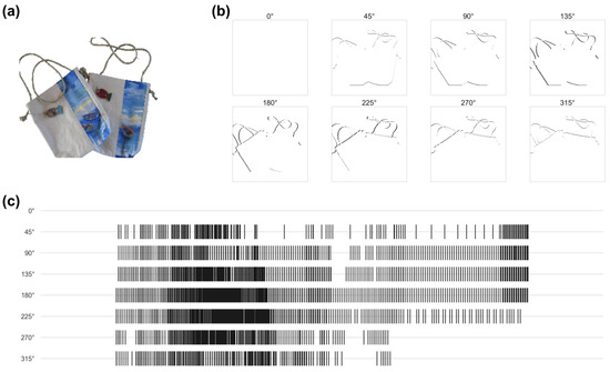
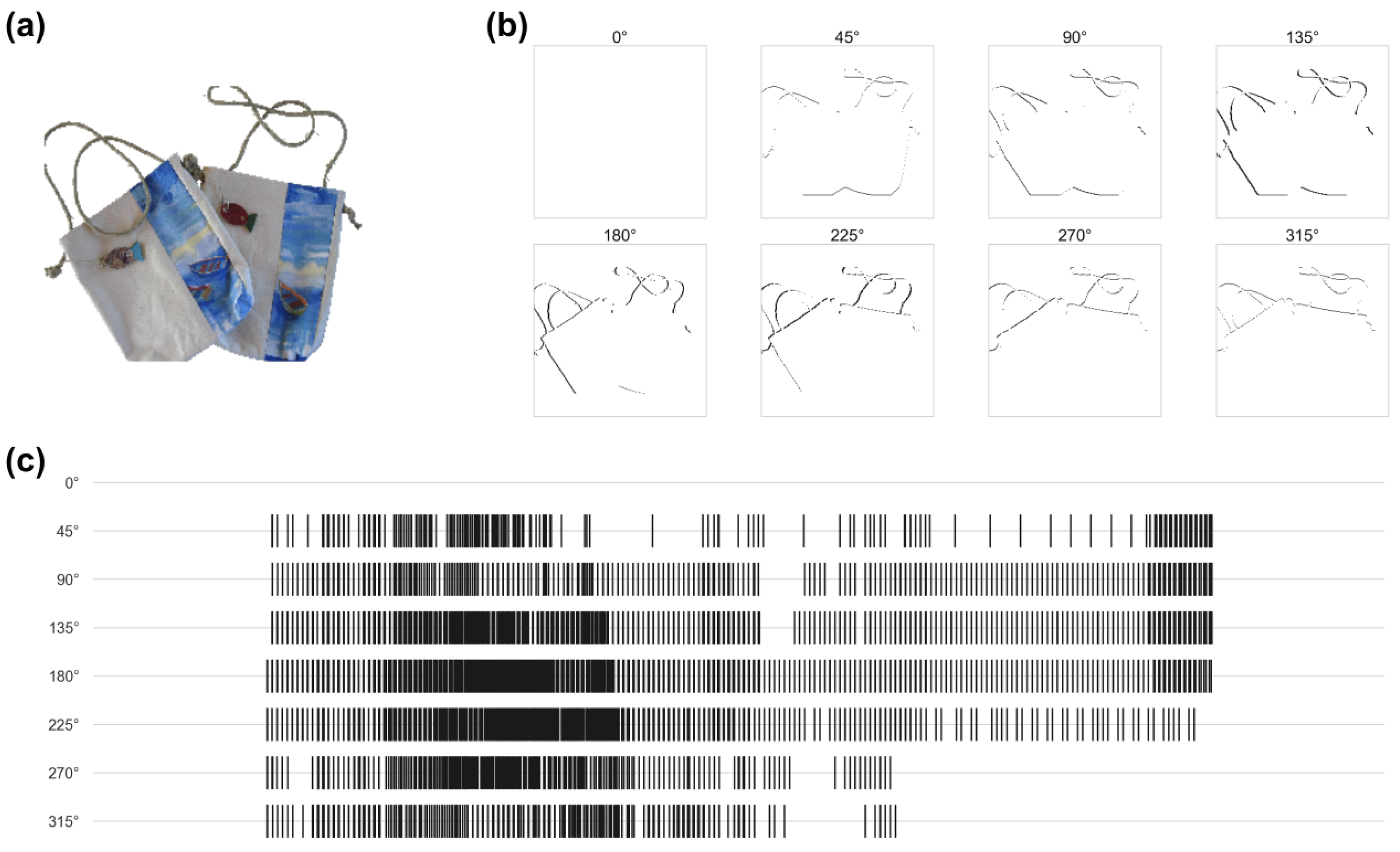
The encoder-only ablation shows that fixed activation-count voting is insufficient for the present cohort, whereas the supplementary localization analysis shows that the pre-decoder code retains direction-indexed spatial structure. Together, these findings motivate learned spatial integration of an inspectable code. Figure 5 visualizes the direction-indexed evidence maps.

Figure 5. Visualization of the neighborhood-indexed evidence code produced by the deterministic inhibitory encoder. (a) Example before/after observation pair. (b) Evidence maps indexed by the first-order lattice-neighborhood hypotheses ${\left\{F^{\left(k\right)}\right\}}_{k=1}^M$. (c) Rasterized view of the ordered neighborhood channels. Angle labels denote the ordered elements of ${\mathcal{N}}_1$ ($M=8$ in the present two-dimensional implementation).

5.1. Scope and Adverse Diagnostic Boundaries

The reported outcomes remain conditional on the declared DIS5K-derived cohort, preprocessing, checkpoints, corruption families, and statistical units. Variation across corruption families and localization tolerances precludes claims of universal robustness, a stable architecture ranking, a new Accuracy ceiling, or general motion-estimation superiority.

The controlled $q=1,\dots ,16$ experiment shows that extending the neuronal detection distance enables the multi-step front end to preserve high average performance from one-pixel motion through the longest evaluated 16-pixel displacement. Its clean/noisy equal-weight Accuracy averages of 0.9949/0.9912 provide direct evidence that DI-Net can perform longer-displacement direction discrimination. However, this panel was designed to isolate the detection-distance extension and therefore only compared S16 with the parameter-matched S1 control, using one training seed and one corruption seed; TSM-MobileNetV2-2f, MaskPair-CNN, and PairLift-CNN v6 were not retrained and evaluated on this $q=1,\dots ,16$ cohort. The result consequently supports the benefit of lengthening the neuronal detection distance, but does not establish cross-architecture superiority. In the supplementary salt-and-pepper ladder (Appendix A.1), the DI-Net/Lucas–Kanade ordering reverses at 10% corruption.

The eleven-method main table includes TSM-MobileNetV2-2f, MaskPair-CNN, and PairLift-CNN v6. TSM is a published external temporal reference but differs in RGB representation, capacity, and training-seed coverage; MaskPair-CNN and PairLift-CNN are author-constructed representation controls rather than external methods. DI-Net is higher than all three on the pooled noisy levels, whereas MaskPair-CNN and PairLift-CNN are slightly higher on clean input. PairLift additionally uses a single post hoc epoch-6 checkpoint selected using clean-training information only. The supplementary paired TSM and five-seed MaskPair analyses retain their narrower statistical interpretations, and none of these results establish a universal architecture ranking. The blur, reciprocal-exposure, and regenerated-rotation results are likewise transformation- and preprocessing-specific rather than evidence of universal distribution-shift robustness.

In the supplementary selected DAVIS-derived task, DI-Net (multi-scale) is the separately DAVIS-trained six-radius extension; it improves over the MaskPair control, while its differences from Lucas–Kanade, Farneback, and RAFT-small remain statistically unresolved. The experiment therefore provides additional evidence on selected natural frames under its stated protocol.

The biological connection remains a discrete logical abstraction rather than a retinal simulation. Original full-scene inputs, predicted masks, segmentation errors, natural occlusion, spatially varying illumination, simultaneous multi-object association, controlled non-rigid deformation, camera motion, general texture variation, and long-sequence temporal consistency remain untested.

5.2. Future Research Directions

Future work should first replace GT object isolation with predicted masks, boundary-perturbed supports, and eventually full-frame inputs so that segmentation-error propagation can be measured explicitly. A second direction is to extend the present multi-step mechanism to longer temporal windows, multiple independently moving objects, non-rigid deformation, occlusion, and camera motion while preserving the direction-indexed semantics of the intermediate code. Third, the multi-step extension should be evaluated with multiple training and corruption seeds and compared directly with TSM-MobileNetV2-2f, MaskPair-CNN, PairLift-CNN, and motion-estimation references on the same $q=1,\dots ,16$ cohort. Finally, uncertainty calibration and failure detection should be incorporated for difficult observation regimes. These directions are prospective and are not implied to have been completed in the present experiments.

6. Conclusions

DI-Net augments an inherited deterministic anti-coincidence code with a compact learned spatial integrator for object-conditioned eight-way direction classification. Under the eleven-method DIS5K main protocol, DI-Net remains competitive with Lucas–Kanade and is higher than TSM-MobileNetV2-2f, MaskPair-CNN, and PairLift-CNN v6 at every pooled noisy level, while the latter two controls are higher on clean input. The full ablation shows complementary contributions from the encoder and decoder across clean, 2.5%, 5%, 7.5%, and 10% conditions. The equal-weight 1–16-pixel results extend the mechanism from minimal motion to longer-displacement direction discrimination, with 0.9949 clean and 0.9912 noisy average Accuracy for the dense multi-step front end. Supplementary experiments in Appendix A.1 provide localization, family-resolved analysis, paired comparator analyses, transformation tests, training-run summaries, and the selected DAVIS-derived evaluation; on the latter task, differences from the three motion references remain statistically unresolved.

The evidence supports an inspectable direction-indexed representation under the evaluated protocols. Segmentation-free full-scene input, predicted-mask errors, multi-object interaction, and long-sequence natural video remain open problems addressed in the preceding future-work subsection.

Appendix A.1. Supplementary Experimental Analyses

The main text presents the DIS5K main comparison, the full component ablation, and the controlled 1–16-pixel multi-step experiment. The following supplementary analyses use separate cohorts, checkpoints, comparison roles, and statistical units; their metrics are not pooled with the main results.

Appendix A.1.1. Family-Resolved DI-Net Analysis

The complete main table pools five impulse families and ten fixed corruption realizations per noisy level. Table A1 reports the four-family DI-Net decomposition; pepper-only remains included in the five-family main panel but is not one of the four rows below.

Table A1. Family-resolved DI-Net performance. Entries are mean [bootstrap 95% CIs] across ten corruption realizations for the fixed seed-42 checkpoint; intervals exclude training-run and test-cohort uncertainty.

Family	Metric	2.5%	5%	7.5%	10%
Block impulse	Accuracy	0.989 [0.988, 0.990]	0.970 [0.969, 0.972]	0.922 [0.920, 0.924]	0.852 [0.849, 0.854]
	Macro-F1	0.989 [0.988, 0.989]	0.970 [0.969, 0.971]	0.922 [0.920, 0.924]	0.849 [0.847, 0.852]
Random-RGB impulse	Accuracy	0.972 [0.971, 0.973]	0.891 [0.890, 0.892]	0.801 [0.800, 0.802]	0.706 [0.704, 0.707]
	Macro-F1	0.972 [0.971, 0.973]	0.892 [0.891, 0.893]	0.802 [0.800, 0.803]	0.704 [0.702, 0.705]
Salt-only	Accuracy	0.971 [0.970, 0.972]	0.893 [0.892, 0.893]	0.801 [0.800, 0.801]	0.706 [0.705, 0.708]
	Macro-F1	0.971 [0.970, 0.972]	0.893 [0.893, 0.894]	0.801 [0.800, 0.802]	0.705 [0.703, 0.706]
Salt-and-pepper	Accuracy	0.983 [0.982, 0.983]	0.922 [0.920, 0.923]	0.827 [0.826, 0.829]	0.717 [0.716, 0.718]
	Macro-F1	0.983 [0.982, 0.983]	0.922 [0.920, 0.923]	0.825 [0.824, 0.827]	0.709 [0.707, 0.710]

Table A1. Family-resolved DI-Net performance. Entries are mean [bootstrap 95% CIs] across ten corruption realizations for the fixed seed-42 checkpoint; intervals exclude training-run and test-cohort uncertainty.

Family	Metric	2.5%	5%	7.5%	10%
Block impulse	Accuracy	0.989 [0.988, 0.990]	0.970 [0.969, 0.972]	0.922 [0.920, 0.924]	0.852 [0.849, 0.854]
	Macro-F1	0.989 [0.988, 0.989]	0.970 [0.969, 0.971]	0.922 [0.920, 0.924]	0.849 [0.847, 0.852]
Random-RGB impulse	Accuracy	0.972 [0.971, 0.973]	0.891 [0.890, 0.892]	0.801 [0.800, 0.802]	0.706 [0.704, 0.707]
	Macro-F1	0.972 [0.971, 0.973]	0.892 [0.891, 0.893]	0.802 [0.800, 0.803]	0.704 [0.702, 0.705]
Salt-only	Accuracy	0.971 [0.970, 0.972]	0.893 [0.892, 0.893]	0.801 [0.800, 0.801]	0.706 [0.705, 0.708]
	Macro-F1	0.971 [0.970, 0.972]	0.893 [0.893, 0.894]	0.801 [0.800, 0.802]	0.705 [0.703, 0.706]
Salt-and-pepper	Accuracy	0.983 [0.982, 0.983]	0.922 [0.920, 0.923]	0.827 [0.826, 0.829]	0.717 [0.716, 0.718]
	Macro-F1	0.983 [0.982, 0.983]	0.922 [0.920, 0.923]	0.825 [0.824, 0.827]	0.709 [0.707, 0.710]

The fixed seed-42 checkpoint ranges from 0.706 Accuracy for random-RGB and salt-only corruption to 0.852 for block impulse at 10%. The supplementary five-run summaries below further show material training-run variation.

Appendix A.1.2. Salt-and-Pepper Comparator Ladder and Training-Run Stability

For the declared independent high-frequency pixel-noise stress test, we selected salt-and-pepper corruption rather than additive Gaussian noise. DI-Net and CNN-from-pair retain their fixed clean-trained seed-42 checkpoints; Lucas–Kanade is deterministic. No method is retrained or adapted to a corruption level.

Table A2. Salt-and-pepper Accuracy and Macro-F1 at four nominal corruption fractions. Each cell is the mean [95% CI] over ten independently keyed corruption realizations on 2470 aligned test pairs; intervals resample corruption realizations and exclude training-run and test-cohort uncertainty.

Method	Metric	2.5%	5%	7.5%	10%
DI-Net	Accuracy	0.983 [0.982, 0.983]	0.922 [0.920, 0.923]	0.827 [0.826, 0.829]	0.717 [0.716, 0.718]
	Macro-F1	0.983 [0.982, 0.983]	0.922 [0.920, 0.923]	0.825 [0.824, 0.827]	0.709 [0.707, 0.710]
CNN-from-pair	Accuracy	0.548 [0.547, 0.549]	0.352 [0.350, 0.353]	0.221 [0.220, 0.222]	0.156 [0.155, 0.156]
	Macro-F1	0.509 [0.508, 0.510]	0.307 [0.305, 0.308]	0.167 [0.166, 0.169]	0.089 [0.088, 0.090]
Lucas–Kanade	Accuracy	0.944 [0.941, 0.946]	0.864 [0.860, 0.868]	0.806 [0.804, 0.809]	0.769 [0.764, 0.774]
	Macro-F1	0.943 [0.941, 0.945]	0.864 [0.860, 0.868]	0.805 [0.803, 0.808]	0.768 [0.763, 0.773]

Table A2. Salt-and-pepper Accuracy and Macro-F1 at four nominal corruption fractions. Each cell is the mean [95% CI] over ten independently keyed corruption realizations on 2470 aligned test pairs; intervals resample corruption realizations and exclude training-run and test-cohort uncertainty.

Method	Metric	2.5%	5%	7.5%	10%
DI-Net	Accuracy	0.983 [0.982, 0.983]	0.922 [0.920, 0.923]	0.827 [0.826, 0.829]	0.717 [0.716, 0.718]
	Macro-F1	0.983 [0.982, 0.983]	0.922 [0.920, 0.923]	0.825 [0.824, 0.827]	0.709 [0.707, 0.710]
CNN-from-pair	Accuracy	0.548 [0.547, 0.549]	0.352 [0.350, 0.353]	0.221 [0.220, 0.222]	0.156 [0.155, 0.156]
	Macro-F1	0.509 [0.508, 0.510]	0.307 [0.305, 0.308]	0.167 [0.166, 0.169]	0.089 [0.088, 0.090]
Lucas–Kanade	Accuracy	0.944 [0.941, 0.946]	0.864 [0.860, 0.868]	0.806 [0.804, 0.809]	0.769 [0.764, 0.774]
	Macro-F1	0.943 [0.941, 0.945]	0.864 [0.860, 0.868]	0.805 [0.803, 0.808]	0.768 [0.763, 0.773]

DI-Net exceeded CNN-from-pair in both metrics at all four levels and exceeded Lucas–Kanade through 7.5% corruption. At 10%, however, Lucas–Kanade was stronger: Accuracy was 0.769 versus 0.717 and Macro-F1 was 0.768 versus 0.709. This crossover precludes a claim of universal high-frequency-noise superiority.

The nominal fraction is an overwrite budget, not a matched receptor-flip rate: point assignments can coincide with original pixel values, while salt/random-RGB can activate the background and block overlap reduces unique coverage. Family results therefore should not be collapsed into a universal robustness ranking.

Across the five runs, clean Accuracy was $99.304\%\pm 0.135\%$. At nominal 10%, family means ranged from 74.136% to 78.204%, and sample SDs from 6.724 to 8.373 percentage points. Clean performance was reproducible, whereas corruption performance depended materially on family and training run.

Table A3. DI-Net stability across five independent training runs. Values are mean ± sample SD across seeds 40–44 after within-run averaging of ten nominal-10% realizations; intervals bootstrap the five run summaries.

Condition	Accuracy (%)	95% CI	Macro-F1 (%)	95% CI
Clean	99.304 ± 0.135	[99.198, 99.409]	99.298 ± 0.133	[99.195, 99.402]
Block impulse	78.204 ± 6.724	[72.193, 82.937]	77.164 ± 8.564	[69.389, 82.632]
Random-RGB impulse	74.139 ± 8.337	[68.306, 80.696]	73.937 ± 9.255	[67.355, 81.962]
Salt-only	74.136 ± 8.373	[68.276, 81.459]	73.925 ± 9.315	[67.311, 81.921]
Salt-and-pepper	76.951 ± 7.113	[72.496, 83.297]	76.621 ± 7.419	[71.746, 83.155]

Table A3. DI-Net stability across five independent training runs. Values are mean ± sample SD across seeds 40–44 after within-run averaging of ten nominal-10% realizations; intervals bootstrap the five run summaries.

Condition	Accuracy (%)	95% CI	Macro-F1 (%)	95% CI
Clean	99.304 ± 0.135	[99.198, 99.409]	99.298 ± 0.133	[99.195, 99.402]
Block impulse	78.204 ± 6.724	[72.193, 82.937]	77.164 ± 8.564	[69.389, 82.632]
Random-RGB impulse	74.139 ± 8.337	[68.306, 80.696]	73.937 ± 9.255	[67.355, 81.962]
Salt-only	74.136 ± 8.373	[68.276, 81.459]	73.925 ± 9.315	[67.311, 81.921]
Salt-and-pepper	76.951 ± 7.113	[72.496, 83.297]	76.621 ± 7.419	[71.746, 83.155]

Appendix A.1.3. Published TSM-MobileNetV2 Two-Frame Comparator

We adapted TSM-MobileNetV2 [33] to two ordered RGB frames and eight direction logits. It was trained from scratch on the same 3000 clean $q=1$ pairs, labels, optimizer family, batch size, 20-epoch budget, and final-epoch rule as DI-Net. Both rows below use the fixed seed 40. TSM has 2,234,120 trainable parameters versus 62,600 for DI-Net and is not capacity-matched.

Table A4. DI-Net and adapted TSM-MobileNetV2-2f on the one-pixel salt-and-pepper ladder. Values are Accuracy/Macro-F1 (%); the two fixed seed-40 checkpoints share the clean cohort and ten fixed corruption realizations.

Method	Clean	S&P 2.5%	S&P 5%	S&P 7.5%	S&P 10%
DI-Net	99.15/99.15	98.63/98.65	94.08/94.18	86.09/86.35	77.99/78.35
TSM-MobileNetV2-2f (adapted)	98.99/98.99	18.49/11.05	14.04/7.06	12.93/5.76	12.72/5.32

Table A4. DI-Net and adapted TSM-MobileNetV2-2f on the one-pixel salt-and-pepper ladder. Values are Accuracy/Macro-F1 (%); the two fixed seed-40 checkpoints share the clean cohort and ten fixed corruption realizations.

Method	Clean	S&P 2.5%	S&P 5%	S&P 7.5%	S&P 10%
DI-Net	99.15/99.15	98.63/98.65	94.08/94.18	86.09/86.35	77.99/78.35
TSM-MobileNetV2-2f (adapted)	98.99/98.99	18.49/11.05	14.04/7.06	12.93/5.76	12.72/5.32

The paired DI-Net-minus-TSM Accuracy difference was +0.16 percentage points on clean input (95% source-stem bootstrap CI [$-0.36$, 0.69]) and +80.14, +80.03, +73.16, and +65.27 points at the four noisy levels. The corresponding intervals were [78.74, 81.51], [78.54, 81.51], [71.36, 74.89], and [63.20, 67.23]. The 20,000 bootstrap replicates resample complete stems while holding both checkpoints and all ten corruption realizations fixed. Consequently, this $T=2$ adaptation is a single-training-seed diagnostic; it does not establish cross-seed stability, statistical significance over training runs, or general superiority to temporal video models.

Table A5. Mixed batch-one engineering profile for DI-Net and TSM-MobileNetV2-2f on one RTX 4060 Laptop GPU. Medians use one fixed clean pair and a counterbalanced schedule; this is not a cross-hardware efficiency ranking.

Method	Parameters	GMAC/Pair	Learned Forward (ms)	Pair Pipeline (ms)
DI-Net	62,600	3.775	1.519 [1.458, 1.580]	12.630 [8.506, 18.729]
TSM-MobileNetV2-2f	2,234,120	0.782	9.456 [9.303, 9.700]	11.681 [11.539, 11.820]

Table A5. Mixed batch-one engineering profile for DI-Net and TSM-MobileNetV2-2f on one RTX 4060 Laptop GPU. Medians use one fixed clean pair and a counterbalanced schedule; this is not a cross-hardware efficiency ranking.

Method	Parameters	GMAC/Pair	Learned Forward (ms)	Pair Pipeline (ms)
DI-Net	62,600	3.775	1.519 [1.458, 1.580]	12.630 [8.506, 18.729]
TSM-MobileNetV2-2f	2,234,120	0.782	9.456 [9.303, 9.700]	11.681 [11.539, 11.820]

The engineering directions are mixed: DI-Net has 35.7 times fewer parameters and a 6.2 times faster learned forward pass, whereas TSM has fewer counted MACs and a slightly lower complete-pipeline point estimate. Four schedule occurrences are engineering repeats, not independent training runs.

Appendix A.1.4. Same-Receptor Learned Control

The primary learned control aligns both capacity and training budget. It compares five DI-Net and five MaskPair-CNN seeds. Table A6 reports clean input and each of the four declared nominal-10% corruption families separately, without cross-family pooling.

Table A6. Five-seed DI-Net and MaskPair-CNN results. Values are mean ± sample SD Accuracy/Macro-F1 (%) over independent training seeds 40–44. Each nominal-10% noisy run summary first averages ten fixed corruption realizations within the same checkpoint and family. The four corruption families are reported separately; no cross-family macro-average is used.

Method	Metric	Clean	Block Impulse	Random RGB	Salt-Only	Salt-and-Pepper
DI-Net	Accuracy	99.304 ± 0.135	78.204 ± 6.724	74.139 ± 8.337	74.136 ± 8.373	76.951 ± 7.113
	Macro-F1	99.298 ± 0.133	77.164 ± 8.564	73.937 ± 9.255	73.925 ± 9.315	76.621 ± 7.419
MaskPair-CNN	Accuracy	99.814 ± 0.289	18.922 ± 4.935	25.640 ± 5.656	25.660 ± 5.654	34.280 ± 7.123
	Macro-F1	99.812 ± 0.292	8.796 ± 4.242	16.235 ± 5.373	16.225 ± 5.354	25.446 ± 8.027

Table A6. Five-seed DI-Net and MaskPair-CNN results. Values are mean ± sample SD Accuracy/Macro-F1 (%) over independent training seeds 40–44. Each nominal-10% noisy run summary first averages ten fixed corruption realizations within the same checkpoint and family. The four corruption families are reported separately; no cross-family macro-average is used.

Method	Metric	Clean	Block Impulse	Random RGB	Salt-Only	Salt-and-Pepper
DI-Net	Accuracy	99.304 ± 0.135	78.204 ± 6.724	74.139 ± 8.337	74.136 ± 8.373	76.951 ± 7.113
	Macro-F1	99.298 ± 0.133	77.164 ± 8.564	73.937 ± 9.255	73.925 ± 9.315	76.621 ± 7.419
MaskPair-CNN	Accuracy	99.814 ± 0.289	18.922 ± 4.935	25.640 ± 5.656	25.660 ± 5.654	34.280 ± 7.123
	Macro-F1	99.812 ± 0.292	8.796 ± 4.242	16.235 ± 5.373	16.225 ± 5.354	25.446 ± 8.027

Across the five training seeds, MaskPair-CNN was higher on clean input by 0.510 Accuracy points and 0.514 Macro-F1 points. Under each of the four declared nominal-10% corruption families, DI-Net had higher mean Accuracy: by 59.282 percentage points for block impulse, 48.499 points for random-RGB impulse, 48.476 points for salt-only corruption, and 42.671 points for salt-and-pepper corruption. Macro-F1 showed the same family-wise ordering. Because only five paired training runs are available, these comparisons are descriptive and are not used to claim conventional cross-run significance or universal representation superiority.

Appendix A.1.5. Additional Deterministic Transformations

We also evaluated the eight main methods on the same 2470 aligned stems under Gaussian blur (radii of 0.5, 1.0, 1.5, and 2.0 pixels), reciprocal spatially uniform temporal exposure changes (0.25, 0.5, 1, and 2 EV, preserving exact black), and label-preserving regenerated rotations (5, 10, 15, and 20 degrees). Fixed clean-trained checkpoints were used without transformation-specific retraining. At the strongest settings, DI-Net Accuracy/Macro-F1 was 0.982/0.982 for blur, 0.991/0.991 for reciprocal exposure, and 0.994/0.993 for regenerated rotation. The outcome is pipeline-specific: at the strongest blur, CNN-from-pair and Lucas–Kanade reached 0.994 and 1.000 Accuracy; at the strongest rotation they reached 0.999 and 1.000. Conversely, at the specified 2 EV exposure transform, DI-Net exceeded both (0.132 and 0.354 Accuracy). Each cell uses one fixed transformation realization, so the results do not quantify transformation-seed, training-seed, or domain uncertainty. Gaussian blur is not additive Gaussian noise, the reciprocal exposure transform is not natural illumination, and regenerated rotation is not general affine robustness.

Appendix A.1.6. DAVIS-Derived Object-Conditioned Multi-Gap Evaluation

To evaluate the mechanism beyond controlled translated-object stimuli, we constructed a selected DAVIS-derived object-conditioned eight-way direction-classification task [46]. The 60 official DAVIS training sequences were partitioned into 48 training and 12 validation sequences before reading images or labels; all 30 official validation sequences formed the sealed test set. This produced 9979 training, 2506 validation, and 5037 test object–frame pairs at temporal gaps $\Delta t\in \{1,2,4,8\}$ and displacement strata of $[2,4)$, $[4,8)$, $[8,16)$, and $[16,32)$ pixels. Annotated objects are isolated on black backgrounds, and annotated-mask centroid displacement is quantized into eight directions. This is not an official DAVIS metric, dense-flow benchmark, or segmentation-free full-frame evaluation.

The target model in this experiment is denoted DI-Net (multi-scale). It uses fixed evidence radii $S=\{1,2,4,8,16,32\}$ and three fixed training seeds (82601–82603). MaskPair-CNN uses the same DAVIS split and seeds. Each learned point estimate is the arithmetic mean of the three checkpoint-specific metrics, not an ensemble prediction. Intervals use 20,000 complete-sequence bootstrap replicates over the 30 test sequences with shared draws for paired contrasts.

Table A7. DAVIS-derived object-conditioned multi-gap eight-way classification. Values are percentages on 5037 test pairs from 30 sequences; brackets give 95% complete-sequence bootstrap intervals. Training and information regimes differ, so this is not an architecture-fair leaderboard.

Method	Training or Diagnostic Role	Accuracy [95% CI]	Macro-F1 [95% CI]
DI-Net (multi-scale)	DAVIS train, three seeds	76.93 [71.37, 81.51]	71.25 [64.97, 75.85]
MaskPair-CNN	DAVIS train, three seeds	70.00 [66.25, 74.32]	62.73 [58.30, 66.51]
Lucas–Kanade	Deterministic sparse flow	77.72 [73.27, 82.17]	73.91 [68.59, 77.72]
Farneback	Deterministic dense flow	76.73 [72.23, 81.24]	72.91 [67.74, 76.59]
RAFT-small	Pretrained C_T_V2 weights	71.21 [67.21, 75.31]	66.30 [61.46, 69.67]

Table A7. DAVIS-derived object-conditioned multi-gap eight-way classification. Values are percentages on 5037 test pairs from 30 sequences; brackets give 95% complete-sequence bootstrap intervals. Training and information regimes differ, so this is not an architecture-fair leaderboard.

Method	Training or Diagnostic Role	Accuracy [95% CI]	Macro-F1 [95% CI]
DI-Net (multi-scale)	DAVIS train, three seeds	76.93 [71.37, 81.51]	71.25 [64.97, 75.85]
MaskPair-CNN	DAVIS train, three seeds	70.00 [66.25, 74.32]	62.73 [58.30, 66.51]
Lucas–Kanade	Deterministic sparse flow	77.72 [73.27, 82.17]	73.91 [68.59, 77.72]
Farneback	Deterministic dense flow	76.73 [72.23, 81.24]	72.91 [67.74, 76.59]
RAFT-small	Pretrained C_T_V2 weights	71.21 [67.21, 75.31]	66.30 [61.46, 69.67]

Within the DAVIS-trained learned group, DI-Net (multi-scale) exceeded MaskPair-CNN by 6.93 Accuracy points (95% paired CI [1.04,11.62]) and 8.51 Macro-F1 points ([1.17,14.85]). This name denotes the separately DAVIS-trained six-radius extension described above. Its paired Accuracy effects relative to Lucas–Kanade, Farneback, and RAFT-small were $-0.79$ [$-6.25$,3.94], +0.20 [$-5.24$,4.82], and +5.72 [$-0.38$,10.45] percentage points; all intervals included zero, so neither superiority nor equivalence was claimed.

Appendix A.2. Complete Experimental Protocols

Four impulse-corruption families were evaluated on already constructed $256\times 256$ RGB observation pairs: salt-and-pepper, salt-only, random RGB impulse, and block impulse. The nominal fraction p is a sampling or overwrite budget over the complete image lattice, including object and background pixels. It is neither foreground relative nor a guarantee that a sampled pixel changes value.

For every point-corruption family and each frame, $\mathrm{round}\left(pHW\right)$ coordinates were sampled uniformly without replacement. Salt-and-pepper corruption set the complete RGB pixel at every selected coordinate to black $(0,0,0)$ or white $(255,255,255)$ with equal probability. Salt-only set the complete pixel to white. Random RGB impulse sampled the three channel values independently from the discrete integers $0,\dots ,255$.

Block impulse used a fixed block width $b=5$ and $\max \{1,\mathrm{round}(pHW/b^2)\}$ block draws per frame. Every top-left origin was sampled uniformly with replacement from $\{0,\dots ,H-b\}\times \{0,\dots ,W-b\}$, so the complete block remained inside the canvas. Each block was set to black or white with equal probability. Origins could repeat and blocks could overlap; later writes replaced earlier values. Realized unique-pixel coverage could therefore be lower than the nominal block budget.

Corruption was introduced only after the clean before/after pair and its one-pixel displacement label had been constructed. The two frames were then corrupted separately using the deterministic key templates seed|family|level|stem|before and seed|family|level|stem|after. The CRC32 of each complete UTF-8 key, interpreted as an unsigned 32-bit value, initialized a NumPy RandomState. The before and after observations consequently used separately generated, independently keyed coordinate and value streams. The same ten corruption-realization identifiers (20260618–20260627) were used for every method and family at each level. Task-trained classifiers were trained only on clean pairs and evaluated from fixed checkpoints; no model was retrained or adapted for a corruption family, fraction, or realization.

The dedicated high-frequency pixel-noise analysis selects salt-and-pepper corruption at $p\in \{0.025,0.05,0.075,0.10\}$ on all 2470 aligned test pairs. Its intervals resample ten fixed corruption-realization summaries for the seed-42 checkpoint; they are not training-run or test-sample intervals.

• Executable order

The protocol can be reproduced without an additional algorithm package by the following ordered operations:

• Select held-out object stem s and applied displacement label y.
• Construct the clean zero-background before observation $B_s$ on the $256\times 256$ canvas.
• Construct the clean after observation $A_s$ by zero-fill translating $B_s$ by the labeled one-pixel displacement y; fix y before any corruption is applied.
• For each frame role $\rho \in \{\mathtt{before},\mathtt{after}\}$, form $k=r\left|f\right|\ell \left|s\right|\rho$, where r is the corruption identifier, f the family, and ℓ the level tag. Initialize RandomState with the unsigned CRC32 value of the complete key.
• For a point family, draw $\mathrm{round}\left(pHW\right)$ coordinates without replacement and overwrite their RGB values according to f. For block impulse, use the draw count in Table A8, sample valid $5\times 5$ origins with replacement, and overwrite each block with a separately sampled black-or-white value.
• Keep y unchanged and provide the identical corrupted RGB pair to all methods before their disclosed method-specific preprocessing.
• For DI-Net, convert each corrupted RGB observation to $P\left(x\right)=⊮[{\max }_c{I}_c\left(x\right)>0]$, construct the eight anti-coincidence channels, normalize the channels by the active after-receptor count, and invoke the fixed-checkpoint CNN decoder.

Table A8. Exact overwrite budgets per frame for the impulse-corruption protocol. Point-family counts are sampled lattice coordinates; block-family counts are $5\times 5$ draws. Block overlap, repeated origins, and assignments equal to the original value can make the realized change smaller than the nominal budget.

Nominal Level	Point Coordinates	$5\times 5$ Block Draws
2.5%	1638	66
5.0%	3277	131
7.5%	4915	197
10.0%	6554	262

Table A8. Exact overwrite budgets per frame for the impulse-corruption protocol. Point-family counts are sampled lattice coordinates; block-family counts are $5\times 5$ draws. Block overlap, repeated origins, and assignments equal to the original value can make the realized change smaller than the nominal budget.

Nominal Level	Point Coordinates	$5\times 5$ Block Draws
2.5%	1638	66
5.0%	3277	131
7.5%	4915	197
10.0%	6554	262

• Protocol scope

The deterministic key construction keeps frame role, family, level, stem, and realization identifier explicit. The results are reported separately by family and level, and the input-generation authority is not treated as a rerun of model inference.

Appendix A.2.1. Supplementary 1–16-Pixel Multi-Step Protocol

The controlled multi-step experiment uses displacement steps $q=1,\dots ,16$, all eight ordered lattice directions, and candidate steps $s=1,\dots ,16$ on a $256\times 256$ canvas. Objects are limited to a 192-pixel bounding box and centered with a 32-pixel margin, satisfying $q_{\max }+s_{\max }=32$. A fixed hash rule selects 512 DIS-TR sources for training, 128 DIS-VD sources for validation, and 128 sources from each of DIS-TE1–4 for the 512-source test cohort. Every source is rendered at all 16 displacement steps and in eight directions. S16 and the widened parameter-matched S1 control use training seed 42, clean training and validation only, and clean validation direction negative log-likelihood for checkpoint selection. The noisy test uses one salt-and-pepper seed (20260618) with 6554 unique spatial coordinates per frame and independently keyed before/after values. Source-cluster intervals use 10,000 paired resamples; the design uses one training seed and one corruption seed.

Appendix A.2.2. Learned-Comparator and Additional-Transformation Protocols

TSM-MobileNetV2-2f consumes the same ordered one-pixel RGB pair and predicts eight logits without dense-flow supervision or flow-to-class binning. It is trained from scratch under the seed-40 DI-Net training cohort, labels, AdamW family, batch size, 20-epoch budget, and final-epoch rule. Its 2,234,120 parameters and RGB input are not capacity- or representation-matched to DI-Net. The TSM bootstrap resamples complete source stems while fixing the two seed-40 checkpoints and the ten corruption realizations.

Figure A1. Representative observations for four illustrated impulse-corruption families. The same held-out DIS5K-derived before/after pair is shown clean and after block impulse, random RGB impulse, salt-only, and salt-and-pepper corruption at the nominal 10% level using corruption identifier 20260618. Each point family samples 6554 of the $256\times 256$ lattice coordinates without replacement per frame. Random RGB impulse draws the three channel values independently from $\{0,\dots ,255\}$; salt-only writes white; and salt-and-pepper writes black or white equiprobably. Block impulse draws 262 valid $5\times 5$ origins with replacement and writes each block black or white equiprobably; overlaps and later-write replacement are therefore possible. Before and after observations use separate deterministic frame-role keys. This pair and realization are illustrative only; reported metrics use all 2470 test pairs and the declared ten corruption-realization identifiers.

Figure A1. Representative observations for four illustrated impulse-corruption families. The same held-out DIS5K-derived before/after pair is shown clean and after block impulse, random RGB impulse, salt-only, and salt-and-pepper corruption at the nominal 10% level using corruption identifier 20260618. Each point family samples 6554 of the $256\times 256$ lattice coordinates without replacement per frame. Random RGB impulse draws the three channel values independently from $\{0,\dots ,255\}$; salt-only writes white; and salt-and-pepper writes black or white equiprobably. Block impulse draws 262 valid $5\times 5$ origins with replacement and writes each block black or white equiprobably; overlaps and later-write replacement are therefore possible. Before and after observations use separate deterministic frame-role keys. This pair and realization are illustrative only; reported metrics use all 2470 test pairs and the declared ten corruption-realization identifiers.

MaskPair-CNN receives the same two $256\times 256$ receptor maps as DI-Net and uses the same Conv–GroupNorm–ReLU widths, global pooling, classifier head, 3000 clean pairs, seeds 40–44, AdamW settings, batch size, 20 fixed epochs, 3760 updates, and final-epoch rule. Its two-channel input differs intentionally from DI-Net’s eight-channel evidence tensor, and its 60,872 parameters are near, not equal to, DI-Net’s 62,600. The nominal-10% family summaries average ten fixed corruption realizations within each training run before computing the five-run mean and sample SD.

PairLift-CNN v6 receives the same two receptor maps, applies a learned bias-free $1\times 1$ two-to-eight-channel lift, and then uses the unchanged DI-Net decoder and head, totaling 62,616 trainable parameters. Its main-panel result uses training seed 40 and a post hoc epoch-6 checkpoint selected using clean-training information only. It is an internal representation diagnostic, not a published external method, a preregistered analysis, a final-epoch-matched comparator, or a multi-seed stability result.

The additional deterministic-transformation analysis uses the same 2470 aligned DIS5K stems and fixed clean-trained checkpoints. Gaussian blur uses 0.5, 1.0, 1.5, and 2.0 radii pixels. Reciprocal temporal exposure applies spatially uniform before/after multiplicative gains corresponding to 0.25, 0.5, 1, and 2 EV while preserving exact black. For regenerated rotation, the clean before frame is rotated by 5, 10, 15, or 20 degrees and the after frame is regenerated by the original labeled integer displacement, preserving the class by construction. Each method–transformation–level cell contains one fixed transformed cohort; no transformation-specific retraining is used.

Appendix A.2.3. DAVIS-Derived Multi-Gap Protocol

The selected DAVIS-derived task partitions the 60 official training sequences into 48 training and 12 validation sequences without image or label access and seals all 30 official validation sequences for testing. Eligible object pairs use temporal gaps $\Delta t\in \{1,2,4,8\}$, annotated-object isolation on black, prespecified trajectory-coherence and direction-quantization gates, and annotated-mask centroid displacement as the eight-way proxy label. DI-Net (multi-scale) uses radii $\{1,2,4,8,16,32\}$; it and MaskPair-CNN are trained on the same DAVIS split with three fixed seeds (82601–82603). The displayed DI-Net (multi-scale) point estimate averages three checkpoint-specific metrics and is not an ensemble prediction. Lucas–Kanade and Farneback are deterministic references, and RAFT-small uses pretrained C_T_V2 weights. Sequence-bootstrap intervals use 20,000 shared draws over the 30 sealed test sequences and do not cover training-seed, selection-gate, or cross-domain uncertainty.

Appendix A.2.4. Localization Protocol

For localization, the target is after-alpha support minus before-alpha support. GT-direction, predicted-direction, and all-channel-union views are evaluated under exact and $L_{\infty }\le 1$ overlap, with count-matched null support sampled inside the after-frame RGB foreground.

Appendix A.2.5. Implementation and Reproducibility Configuration

The learned decoder follows Section 3.4: three $3\times 3$ convolutional blocks with channel widths $M\to 32\to 64\to 64$ ($M=8$), with each block applying Group Normalization with $g=8$ groups followed by ReLU, then global average pooling and a two-layer head $64\to 64\to M$; dropout with $p=0.1$ is applied to the pooled features before the head, as in Equation (7). The original decoder uses cross-entropy and AdamW (learning rate $5\times {10}^{-4}$, weight decay ${10}^{-4}$), a batch size of 16, a constant learning rate, and a fixed 20-epoch budget. It is trained from scratch without online geometric, photometric, corruption, MixUp, or CutMix augmentation; no scheduler, automated search, early stopping, or held-out checkpoint selection is used, and the final epoch is retained. The historical main checkpoint uses seed 42; the stability study uses seeds 40–44.

The formal accuracy evaluation used Windows 10.0.26200, Python 3.10.6, PyTorch 2.1.2+cu121, torchvision 0.16.2+cu121, NumPy 1.26.4, Pillow 12.1.0, and OpenCV 4.13.0.90 on an NVIDIA GeForce RTX 4060 Laptop GPU. The CPU latency audit used a 13th Gen Intel Core i9-13900HX. The complete environment of the historical seed-42 training and 646.1 samples/s profile was not preserved, so later software details are not assigned retrospectively.

Table A9. Learned-module profiles for the target model and raw-pair component ablation on an RTX 4060 Laptop GPU. Batch-one random tensors and different input shapes were used. Receptor conversion, deterministic encoding, transfer, file I/O, and postprocessing are excluded; this is not end-to-end throughput.

Profiled Learned Module	Input	Params (M)	Profiler GFLOPs	Samples/s	Peak Allocated (MiB)
DI-Net CNN decoder	$1\times 8\times 256\times 256$	0.063	7.550	646.1	58.5
CNN-from-pair	$1\times 6\times 299\times 299$	0.062	10.196	441.2	76.4

Table A9. Learned-module profiles for the target model and raw-pair component ablation on an RTX 4060 Laptop GPU. Batch-one random tensors and different input shapes were used. Receptor conversion, deterministic encoding, transfer, file I/O, and postprocessing are excluded; this is not end-to-end throughput.

Profiled Learned Module	Input	Params (M)	Profiler GFLOPs	Samples/s	Peak Allocated (MiB)
DI-Net CNN decoder	$1\times 8\times 256\times 256$	0.063	7.550	646.1	58.5
CNN-from-pair	$1\times 6\times 299\times 299$	0.062	10.196	441.2	76.4

The 646.1 samples/s row profiles the decoder on a random GPU-resident tensor without a loaded checkpoint. Audited CPU component latency records are reported in Appendix A.4. No cross-hardware speedup or universal efficiency ranking is inferred.

Appendix A.3. Complete Comparator Configurations and Comparison Roles

All evaluated methods predict the same eight applied-displacement classes, but they do not all match receptor source, representation, capacity, training, or support access. Table A10 and Table A11 disclose the executed settings; Table A12 isolates the primary fairness comparison.

Table A10. Executed configurations and roles for DI-Net and the learned or deterministic-code comparators. 

Method	Task Input and Preprocessing	Initialization/Capacity	Task Training and Reported Checkpoint	Inference Aggregation and Role
DI-Net	Eight-channel directional code, $256\times 256$	From scratch; 62,600 trainable parameters	Seed 42 for fixed-checkpoint tables and seeds 40–44 for the matched-control analysis; AdamW, $5\times {10}^{-4}$, WD ${10}^{-4}$; batch 16; 20 epochs; final epoch	Eight logits; target method
Encoder-only	Same normalized directional code as DI-Net, followed by channel sums	No learned decoder or trainable decision parameters	No task training or checkpoint selection	Lowest-index $\arg \max$; protocol-aligned 2021 predecessor readout and decoder-removal ablation
CNN-from-pair	Concatenated RGB pair, $6\times 299\times 299$	From scratch; 62,024 parameters	Same optimizer and 20-epoch budget as DI-Net; train-clean Macro-F1 checkpoint, epoch 6	Historical same-backbone and near-capacity ablation; input resolution and FLOPs differ
MaskPair-CNN	Two receptor maps, $2\times 256\times 256$	From scratch; 60,872 parameters	Seeds 40–44; same data, AdamW settings, batch 16, 20 epochs, 3760 updates, and final-epoch rule as DI-Net	Same-receptor, same-resolution, near-capacity, equal-budget learned control; tensor differs intentionally
PairLift-CNN v6	Two receptor maps; learned bias-free $1\times 1$ lift to eight channels	From scratch; 62,616 parameters	Seed 40; post hoc epoch-6 checkpoint selected using clean-training information only	Internal representation control; not preregistered, multi-seed, or final-epoch-matched
TSM-MobileNetV2-2f	Ordered RGB pair, $2\times 3\times 256\times 256$; $[0,1]$ scaling and ImageNet mean/SD normalization; no resize or augmentation	From scratch; 2,234,120 parameters; offline bidirectional TSM ($T=2$, shift divisor 8) in ten MobileNetV2 residual blocks	Seed 40; same 3000 clean pairs/labels, AdamW settings, batch 16, 20 epochs, 3760 updates, and final-epoch rule	Mean of two frame logits; adapted published temporal reference, task/budget-aligned but not representation/capacity-matched

Table A10. Executed configurations and roles for DI-Net and the learned or deterministic-code comparators. 

Method	Task Input and Preprocessing	Initialization/Capacity	Task Training and Reported Checkpoint	Inference Aggregation and Role
DI-Net	Eight-channel directional code, $256\times 256$	From scratch; 62,600 trainable parameters	Seed 42 for fixed-checkpoint tables and seeds 40–44 for the matched-control analysis; AdamW, $5\times {10}^{-4}$, WD ${10}^{-4}$; batch 16; 20 epochs; final epoch	Eight logits; target method
Encoder-only	Same normalized directional code as DI-Net, followed by channel sums	No learned decoder or trainable decision parameters	No task training or checkpoint selection	Lowest-index $\arg \max$; protocol-aligned 2021 predecessor readout and decoder-removal ablation
CNN-from-pair	Concatenated RGB pair, $6\times 299\times 299$	From scratch; 62,024 parameters	Same optimizer and 20-epoch budget as DI-Net; train-clean Macro-F1 checkpoint, epoch 6	Historical same-backbone and near-capacity ablation; input resolution and FLOPs differ
MaskPair-CNN	Two receptor maps, $2\times 256\times 256$	From scratch; 60,872 parameters	Seeds 40–44; same data, AdamW settings, batch 16, 20 epochs, 3760 updates, and final-epoch rule as DI-Net	Same-receptor, same-resolution, near-capacity, equal-budget learned control; tensor differs intentionally
PairLift-CNN v6	Two receptor maps; learned bias-free $1\times 1$ lift to eight channels	From scratch; 62,616 parameters	Seed 40; post hoc epoch-6 checkpoint selected using clean-training information only	Internal representation control; not preregistered, multi-seed, or final-epoch-matched
TSM-MobileNetV2-2f	Ordered RGB pair, $2\times 3\times 256\times 256$; $[0,1]$ scaling and ImageNet mean/SD normalization; no resize or augmentation	From scratch; 2,234,120 parameters; offline bidirectional TSM ($T=2$, shift divisor 8) in ten MobileNetV2 residual blocks	Seed 40; same 3000 clean pairs/labels, AdamW settings, batch 16, 20 epochs, 3760 updates, and final-epoch rule	Mean of two frame logits; adapted published temporal reference, task/budget-aligned but not representation/capacity-matched

Historical raw-pair training used CUDA automatic mixed precision with TF32 disabled; the recorded evaluation used evaluation mode, FP32 tensors without autocast, no gradients or test-time augmentation, and a batch size of 8.

• Common motion-vector quantization

For the three motion references, OpenCV/flow components $(d_x,d_y)$ are reordered to $(d_y,d_x)$ and mapped by cosine similarity to

$$\begin{array}{cc}\hfill \mathcal{D}=\{& (0,1),(1,1),(1,0),(1,-1),\hfill \\ & (0,-1),(-1,-1),(-1,0),(-1,1)\},\hfill \\ \hfill \widehat{k}=& \arg \underset{k}{\max }{\displaystyle \frac{(d_y,d_x)·{\mathcal{D}}_k}{{\parallel (d_y,d_x)\parallel }_2{\parallel {\mathcal{D}}_k\parallel }_2}},\hfill \end{array}$$

where image y increases downward and ties take the lowest index. No angular tolerance is applied.

Table A11. Executed configurations for support-assisted motion references on the 5037-pair DAVIS-derived test. 

Method	Input/Support and Estimator	Vector Aggregation	Failure Rule and Role
Lucas–Kanade	RGB-to-gray; Shi–Tomasi points inside before-frame any-RGB-nonzero support (max of 512, quality of 0.01, distance of 3, block of 3); pyramidal LK window $21\times 21$, max level of 3, 30 iterations, $ϵ=0.01$	Status-valid tracks only; component-wise median displacement, then common eight-direction rule	Missing/empty or zero/non-finite median maps to class 0 (3/5037); deterministic sparse-flow reference
Farneback	RGB-to-gray; dense flow with pyramid scale 0.5, four levels, window 21, five iterations, polynomial neighborhood of 7, $\sigma =1.5$, zero flags	Component-wise median over before-frame any-RGB-nonzero support, then common rule	Invalid median would map to class 0 (0/5037 observed); deterministic dense-flow reference
RAFT-small	Torchvision RAFT-small C_T_V2 weights; RGB $[0,1]$ plus weight transforms; bilinear pad-resize to multiples of eight and vector-rescaled return to the original canvas; batch four	Final predicted flow; finite vectors inside the union of before/after any-RGB-nonzero supports; component-wise median, then common rule	Empty/non-finite/zero aggregate falls back to support-centroid displacement and then eight-shift Dice matching; pretrained dense-flow reference

Table A11. Executed configurations for support-assisted motion references on the 5037-pair DAVIS-derived test. 

Method	Input/Support and Estimator	Vector Aggregation	Failure Rule and Role
Lucas–Kanade	RGB-to-gray; Shi–Tomasi points inside before-frame any-RGB-nonzero support (max of 512, quality of 0.01, distance of 3, block of 3); pyramidal LK window $21\times 21$, max level of 3, 30 iterations, $ϵ=0.01$	Status-valid tracks only; component-wise median displacement, then common eight-direction rule	Missing/empty or zero/non-finite median maps to class 0 (3/5037); deterministic sparse-flow reference
Farneback	RGB-to-gray; dense flow with pyramid scale 0.5, four levels, window 21, five iterations, polynomial neighborhood of 7, $\sigma =1.5$, zero flags	Component-wise median over before-frame any-RGB-nonzero support, then common rule	Invalid median would map to class 0 (0/5037 observed); deterministic dense-flow reference
RAFT-small	Torchvision RAFT-small C_T_V2 weights; RGB $[0,1]$ plus weight transforms; bilinear pad-resize to multiples of eight and vector-rescaled return to the original canvas; batch four	Final predicted flow; finite vectors inside the union of before/after any-RGB-nonzero supports; component-wise median, then common rule	Empty/non-finite/zero aggregate falls back to support-centroid displacement and then eight-shift Dice matching; pretrained dense-flow reference

Table A12. Primary fairness design: DI-Net versus MaskPair-CNN. Only the representation presented to the matched CNN is intentionally changed.

Design Dimension	DI-Net	MaskPair-CNN
Upstream information	Same ordered any-RGB-nonzero receptor maps $P^{-},P^{+}$	Same ordered maps $P^{-},P^{+}$
Network input	Eight-channel normalized anti-coincidence tensor $\mathbf{F}\in {\mathbb{R}}^{8\times 256\times 256}$	Stacked receptor pair $[P^{-},P^{+}]\in {\{0,1\}}^{2\times 256\times 256}$
Backbone and head	Three Conv–GroupNorm–ReLU blocks, global pooling, eight-class head	Same widths, normalization, activation, pooling, and head
Trainable parameters	62,600	60,872 (near-capacity, not exact-capacity)
Data and runs	Same 3000 clean pairs and labels; seeds 40–44	Same 3000 clean pairs and labels; seeds 40–44
Optimization and selection	AdamW, $5\times {10}^{-4}$, WD ${10}^{-4}$, batch 16, 20 epochs/3760 updates, final epoch	Identical optimizer, batch, epoch/update budget, and final-epoch rule
Comparison question	Target model	Effect of the directional anti-coincidence representation under matched receptors and training

Table A12. Primary fairness design: DI-Net versus MaskPair-CNN. Only the representation presented to the matched CNN is intentionally changed.

Design Dimension	DI-Net	MaskPair-CNN
Upstream information	Same ordered any-RGB-nonzero receptor maps $P^{-},P^{+}$	Same ordered maps $P^{-},P^{+}$
Network input	Eight-channel normalized anti-coincidence tensor $\mathbf{F}\in {\mathbb{R}}^{8\times 256\times 256}$	Stacked receptor pair $[P^{-},P^{+}]\in {\{0,1\}}^{2\times 256\times 256}$
Backbone and head	Three Conv–GroupNorm–ReLU blocks, global pooling, eight-class head	Same widths, normalization, activation, pooling, and head
Trainable parameters	62,600	60,872 (near-capacity, not exact-capacity)
Data and runs	Same 3000 clean pairs and labels; seeds 40–44	Same 3000 clean pairs and labels; seeds 40–44
Optimization and selection	AdamW, $5\times {10}^{-4}$, WD ${10}^{-4}$, batch 16, 20 epochs/3760 updates, final epoch	Identical optimizer, batch, epoch/update budget, and final-epoch rule
Comparison question	Target model	Effect of the directional anti-coincidence representation under matched receptors and training

ResNet-50 and MaxViT-tiny provide historical main-panel context in Table 4, but they are not treated as quantitative fairness evidence because their runs differ in pretraining, raw-pair representation, resolution, capacity, preprocessing, optimization/update budget, and checkpoint selection; we make no inference that larger pretrained models are intrinsically inferior.

Appendix A.4. Statistical Units and Reproducibility Records

The analysis keeps three design entities separate. A training run is an independent initialization and shuffle followed by the complete 20-epoch training protocol and final-epoch checkpoint. A corruption realization is one prespecified deterministic identifier used to generate a family- and frame-specific perturbation for a fixed checkpoint. An aligned stem is the same held-out object-pair identity evaluated by each compared method under the same condition. Corruption realizations are not relabeled as training runs, and the corruption families are experimental strata rather than random draws from one noise population.

For fixed-checkpoint family/level summaries, ten realization-level metrics are averaged within the family and a percentile interval is formed from 20,000 bootstrap resamples of those ten summaries. This interval describes corruption-realization variation for that fixed checkpoint; it does not contain training-run, test-cohort, dataset, or domain uncertainty. For independent training analysis at nominal 10%, the order is reversed only after respecting the hierarchy: the ten realizations are first averaged within each checkpoint and family, producing one summary ${\overline{M}}_{t,f}$ for every training run t and family f. Mean and sample SD are then computed over seeds 40–44, with

$${\overline{M}}_f={\displaystyle \frac{1}{5}}{\displaystyle \sum _{t=40}^{44}}{\overline{M}}_{t,f},s_f=\sqrt{{\displaystyle \frac{1}{4}}\sum _{t=40}^{44}{({\overline{M}}_{t,f}-{\overline{M}}_f)}^2}.$$

The DI-Net-only family intervals use 50,000 percentile-bootstrap resamples of the five run-level summaries. Family identity is never pooled into realization or training-run variance. No cross-training-run significance claim is made.

Table A13. Complete DI-Net results for five independent training runs. Each noisy cell is percentage Accuracy/Macro-F1 after averaging the ten nominal-10% corruption realizations within that checkpoint and family.

Seed	Clean	Block Impulse	Random RGB	Salt-Only	Salt-and-Pepper
40	99.150/99.155	67.231/62.621	77.943/79.167	77.951/79.176	77.980/78.340
41	99.393/99.385	77.818/77.778	86.709/86.785	86.721/86.792	88.935/88.859
42	99.312/99.295	85.162/84.924	70.559/70.370	70.636/70.454	71.700/70.857
43	99.474/99.471	79.356/79.194	70.077/70.695	70.138/70.765	73.202/73.080
44	99.190/99.184	81.453/81.303	65.409/62.669	65.235/62.439	72.939/71.968

Table A13. Complete DI-Net results for five independent training runs. Each noisy cell is percentage Accuracy/Macro-F1 after averaging the ten nominal-10% corruption realizations within that checkpoint and family.

Seed	Clean	Block Impulse	Random RGB	Salt-Only	Salt-and-Pepper
40	99.150/99.155	67.231/62.621	77.943/79.167	77.951/79.176	77.980/78.340
41	99.393/99.385	77.818/77.778	86.709/86.785	86.721/86.792	88.935/88.859
42	99.312/99.295	85.162/84.924	70.559/70.370	70.636/70.454	71.700/70.857
43	99.474/99.471	79.356/79.194	70.077/70.695	70.138/70.765	73.202/73.080
44	99.190/99.184	81.453/81.303	65.409/62.669	65.235/62.439	72.939/71.968

Across the five parameter-distinct checkpoints, clean DI-Net performance is consistent, but nominal-10% family Accuracy SDs range from 6.724 to 8.373 percentage points. The run summaries are formed only after averaging the ten realizations within each checkpoint and family; clean reproducibility therefore does not imply training-run-invariant corrupted performance.

Appendix A.4.1. Complete Localization Views

The motion-leading target is the after-frame alpha support minus the before-frame alpha support. The frozen model’s predicted-direction channel is evaluated under exact and one-pixel Chebyshev tolerances. The null is count-matched within each after-frame RGB support; intervals use 20,000 stem bootstrap resamples over 2470 pairs. The predicted-direction evidence is enriched above the support-conditioned null under both definitions, with exact precision/recall of 0.529/0.865 and one-pixel-tolerant precision/recall of 0.986/0.980.

Table A14. Complete evidence view and tolerance analysis for localization. Values are point estimates (95% complete-stem bootstrap intervals).

Evidence View	Tolerance	Precision	Recall	Conditional Null	Enrichment
GT-direction	exact	0.530 (0.526–0.533)	0.867 (0.860–0.873)	0.173 (0.166–0.180)	3.063 (2.954–3.178)
GT-direction	$L_{\infty }\le 1$	0.986 (0.984–0.989)	0.982 (0.980–0.983)	0.359 (0.348–0.371)	2.746 (2.663–2.835)
Predicted-direction	exact	0.529 (0.525–0.533)	0.865 (0.858–0.871)	0.173 (0.166–0.180)	3.066 (2.957–3.181)
Predicted-direction	$L_{\infty }\le 1$	0.986 (0.984–0.989)	0.980 (0.977–0.983)	0.359 (0.347–0.370)	2.750 (2.666–2.838)
All-channel union	exact	0.364 (0.358–0.369)	0.966 (0.964–0.968)	0.160 (0.154–0.166)	2.279 (2.215–2.348)
All-channel union	$L_{\infty }\le 1$	0.818 (0.812–0.824)	0.996 (0.995–0.997)	0.343 (0.332–0.353)	2.386 (2.323–2.453)

Table A14. Complete evidence view and tolerance analysis for localization. Values are point estimates (95% complete-stem bootstrap intervals).

Evidence View	Tolerance	Precision	Recall	Conditional Null	Enrichment
GT-direction	exact	0.530 (0.526–0.533)	0.867 (0.860–0.873)	0.173 (0.166–0.180)	3.063 (2.954–3.178)
GT-direction	$L_{\infty }\le 1$	0.986 (0.984–0.989)	0.982 (0.980–0.983)	0.359 (0.348–0.371)	2.746 (2.663–2.835)
Predicted-direction	exact	0.529 (0.525–0.533)	0.865 (0.858–0.871)	0.173 (0.166–0.180)	3.066 (2.957–3.181)
Predicted-direction	$L_{\infty }\le 1$	0.986 (0.984–0.989)	0.980 (0.977–0.983)	0.359 (0.347–0.370)	2.750 (2.666–2.838)
All-channel union	exact	0.364 (0.358–0.369)	0.966 (0.964–0.968)	0.160 (0.154–0.166)	2.279 (2.215–2.348)
All-channel union	$L_{\infty }\le 1$	0.818 (0.812–0.824)	0.996 (0.995–0.997)	0.343 (0.332–0.353)	2.386 (2.323–2.453)

The all-channel union increases recall at the cost of spatial specificity. GT-selected and predicted-channel aggregates are close partly because the frozen checkpoint classifies 2453 of 2470 stems correctly. Three stems have no positive predicted-channel support. These results concern positive pre-decoder support only.

Appendix A.4.2. CPU Component Latency

Table A15. Audited CPU component latency on an Intel Core i9-13900HX. Each row uses 32 real direction-stratified pairs, five passes, a batch size of one, one warm-up pass, and one PyTorch intra-/inter-op thread.

Measured Scope	Median (ms)	Mean (ms)
Two-PNG decoder and receptor conversion	2.307	2.421
Deterministic encoder, predecoded receptors	1.107	1.272
Seed-42 decoder, resident evidence tensor	84.736	84.915
Warm-cache PNG-to-argmax path	89.957	90.083

Table A15. Audited CPU component latency on an Intel Core i9-13900HX. Each row uses 32 real direction-stratified pairs, five passes, a batch size of one, one warm-up pass, and one PyTorch intra-/inter-op thread.

Measured Scope	Median (ms)	Mean (ms)
Two-PNG decoder and receptor conversion	2.307	2.421
Deterministic encoder, predecoded receptors	1.107	1.272
Seed-42 decoder, resident evidence tensor	84.736	84.915
Warm-cache PNG-to-argmax path	89.957	90.083

References

- Kandel, E.R.; Schwartz, J.H.; Jessell, T.M.; Siegelbaum, S.A.; Hudspeth, A.J. Principles of Neural Science, 5th ed.; McGraw-Hill: New York, NY, USA, 2013. [Google Scholar]
- Meister, M.; Berry, M.J. The neural code of the retina. Neuron 1999, 22, 435–450. [Google Scholar] [CrossRef] [Scilit] [PubMed]
- Gollisch, T.; Meister, M. Eye smarter than scientists believed: Neural computations in circuits of the retina. Neuron 2010, 65, 150–164. [Google Scholar] [CrossRef] [Scilit] [PubMed]
- Masland, R.H. The neuronal organization of the retina. Neuron 2012, 76, 266–284. [Google Scholar] [CrossRef] [Scilit] [PubMed]
- Baden, T.; Berens, P.; Franke, K.; Román Rosón, M.; Bethge, M.; Euler, T. The functional diversity of retinal ganglion cells in the mouse. Nature 2016, 529, 345–350. [Google Scholar] [CrossRef] [Scilit] [PubMed]
- Sterling, P.; Laughlin, S. Principles of Neural Design; MIT Press: Cambridge, MA, USA, 2015. [Google Scholar]
- Wei, W. Neural Mechanisms of Motion Processing in the Mammalian Retina. Annu. Rev. Vis. Sci. 2018, 4, 165–192. [Google Scholar] [CrossRef] [Scilit] [PubMed]
- Hassabis, D.; Kumaran, D.; Summerfield, C.; Botvinick, M. Neuroscience-inspired artificial intelligence. Neuron 2017, 95, 245–258. [Google Scholar] [CrossRef] [Scilit] [PubMed]
- Zador, A.M. A critique of pure learning and what artificial neural networks can learn from animal brains. Nat. Commun. 2019, 10, 3770. [Google Scholar] [CrossRef] [Scilit] [PubMed]
- Richards, B.A.; Lillicrap, T.P.; Beaudoin, P.; Bengio, Y.; Bogacz, R.; Christensen, A.; Clopath, C.; Costa, R.P.; de Berker, A.; Ganguli, S.; et al. A deep learning framework for neuroscience. Nat. Neurosci. 2019, 22, 1761–1770. [Google Scholar] [CrossRef] [Scilit] [PubMed]
- Briggman, K.L.; Helmstaedter, M.; Denk, W. Wiring specificity in the direction-selectivity circuit of the retina. Nature 2011, 471, 183–188. [Google Scholar] [CrossRef] [Scilit] [PubMed]
- Vaney, D.I.; Sivyer, B.; Taylor, W.R. Direction selectivity in the retina: Symmetry and asymmetry in structure and function. Nat. Rev. Neurosci. 2012, 13, 194–208. [Google Scholar] [CrossRef] [Scilit] [PubMed]
- Borst, A.; Helmstaedter, M. Common circuit design in fly and mammalian motion vision. Nat. Neurosci. 2015, 18, 1067–1076. [Google Scholar] [CrossRef] [Scilit] [PubMed]
- Barlow, H.B.; Levick, W.R. The mechanism of directionally selective units in rabbit’s retina. J. Physiol. 1965, 178, 477–504. [Google Scholar] [CrossRef] [Scilit] [PubMed]
- Torre, V.; Poggio, T.A. A synaptic mechanism possibly underlying directional selectivity to motion. Proc. R. Soc. Lond. Ser. B Biol. Sci. 1978, 202, 409–416. [Google Scholar] [CrossRef] [Scilit]
- Adelson, E.H.; Bergen, J.R. Spatiotemporal Energy Models for the Perception of Motion. J. Opt. Soc. Am. A 1985, 2, 284–299. [Google Scholar] [CrossRef] [Scilit] [PubMed]
- Huang, X.; Qiao, H.; Li, H.; Jiang, Z. A Bioinspired Retinal Neural Network for Accurately Extracting Small-Target Motion Information in Cluttered Backgrounds. Image Vis. Comput. 2021, 114, 104266. [Google Scholar] [CrossRef] [Scilit]
- Hua, Y.; Todo, Y.; Tao, S.; Tang, Z.; Cheng, T.; Qiu, Z. Bio-Inspired Computational Model for Direction and Speed Detection. Knowl.-Based Syst. 2024, 300, 112195. [Google Scholar] [CrossRef] [Scilit]
- Tao, S.; Zhao, R.; Yang, Y.; Todo, H.; Tang, Z.; Todo, Y. Artificial Visual Network with Fully Modeled Retinal Direction-Selective Neural Pathway for Motion Direction Detection in Grayscale Scenes. Symmetry 2024, 16, 1592. [Google Scholar] [CrossRef] [Scilit]
- Baek, E.; Song, S.; Baek, C.K.; Rong, Z.; Shi, L.; Cannistraci, C.V. Neuromorphic Dendritic Network Computation with Silent Synapses for Visual Motion Perception. Nat. Electron. 2024, 7, 454–465. [Google Scholar] [CrossRef] [Scilit]
- Han, M.; Todo, Y.; Tang, Z. Mechanism of motion direction detection based on Barlow’s retina inhibitory scheme in direction-selective ganglion cells. Electronics 2021, 10, 1663. [Google Scholar] [CrossRef] [Scilit]
- Li, B.; Todo, Y.; Tang, Z.; Tang, C. The mechanism of orientation detection based on color-orientation jointly selective cells. Knowl.-Based Syst. 2022, 254, 109715. [Google Scholar] [CrossRef] [Scilit]
- Chen, T.; Qiu, Z.; Hua, Y.; Todo, Y.; Tang, Z. Learning orientation detection system and its application to RGB images. In Proceedings of the International Conference on Optics, Electronics, and Communication Engineering, Wuhan, China, 26–28 July 2024; SPIE: Bellingham, WA, USA, 2024; Volume 13395, p. 1339521. [Google Scholar] [CrossRef] [Scilit]
- Dapello, J.; Marques, T.; Schrimpf, M.; Geiger, F.; Cox, D.D.; DiCarlo, J.J. Simulating a Primary Visual Cortex at the Front of CNNs Improves Robustness to Image Perturbations. In Proceedings of the Advances in Neural Information Processing Systems, Virtual Conference, 6–12 December 2020; Volume 33, pp. 13073–13087. [Google Scholar]
- Wang, Y.; Li, B.; Todo, Y. Enhancing robustness of object detection: Hubel–Wiesel model connected with deep learning. Knowl.-Based Syst. 2025, 311, 112984. [Google Scholar] [CrossRef] [Scilit]
- Li, J.; Lei, Z.; Zhang, Z.; Li, H.; Todo, Y.; Gao, S. Alternating excitation–inhibition dendritic computing for classification. IEEE Trans. Artif. Intell. 2024, 5, 5431–5441. [Google Scholar] [CrossRef] [Scilit]
- Sun, Z.; Chen, Y.J.; Yang, Y.H.; Li, Y.; Nishida, S. Machine Learning Modelling for Multi-Order Human Visual Motion Processing. Nat. Mach. Intell. 2025, 7, 1037–1052. [Google Scholar] [CrossRef] [Scilit]
- Chen, T.; Kobayashi, Y.; Todo, Y.; Tang, Z. A learning artificial visual system for motion direction detection. Neural Comput. Appl. 2024, 36, 17181–17197. [Google Scholar] [CrossRef] [Scilit]
- Chen, T.; Todo, Y.; Qiu, Z.; Hua, Y.; Sugiura, H.; Tang, Z. A Bio-Inspired Learning Dendritic Motion Detection Framework with Direction-Selective Horizontal Cells. Biomimetics 2025, 10, 286. [Google Scholar] [CrossRef] [Scilit] [PubMed]
- Qiu, Z.; Hua, Y.; Chen, T.; Todo, Y.; Tang, Z.; Qiu, D.; Chu, C. A Gaussian Mixture Model-Based Unsupervised Dendritic Artificial Visual System for Motion Direction Detection. Biomimetics 2025, 10, 332. [Google Scholar] [CrossRef] [Scilit] [PubMed]
- Roy, K.; Jaiswal, A.; Panda, P. Towards spike-based machine intelligence with neuromorphic computing. Nature 2019, 575, 607–617. [Google Scholar] [CrossRef] [Scilit] [PubMed]
- Gallego, G.; Delbrück, T.; Orchard, G.; Bartolozzi, C.; Taba, B.; Censi, A.; Leutenegger, S.; Davison, A.J.; Conradt, J.; Daniilidis, K.; et al. Event-Based Vision: A Survey. IEEE Trans. Pattern Anal. Mach. Intell. 2022, 44, 154–180. [Google Scholar] [CrossRef] [Scilit] [PubMed]
- Lin, J.; Gan, C.; Han, S. TSM: Temporal Shift Module for Efficient Video Understanding. In Proceedings of the IEEE/CVF International Conference on Computer Vision, Seoul, Republic of Korea, 27 October–2 November 2019; pp. 7083–7093. [Google Scholar] [CrossRef] [Scilit]
- Horn, B.K.P.; Schunck, B.G. Determining Optical Flow. Artif. Intell. 1981, 17, 185–203. [Google Scholar] [CrossRef] [Scilit]
- Lucas, B.D.; Kanade, T. An Iterative Image Registration Technique with an Application to Stereo Vision. In Proceedings of the 7th International Joint Conference on Artificial Intelligence (IJCAI), Vancouver, BC, Canada, 24–28 August 1981; pp. 674–679. [Google Scholar]
- Farnebäck, G. Two-Frame Motion Estimation Based on Polynomial Expansion. In Proceedings of the Image Analysis: 13th Scandinavian Conference, SCIA 2003; Lecture Notes in Computer Science; Springer: Berlin/Heidelberg, Germany, 2003; Volume 2749, pp. 363–370. [Google Scholar] [CrossRef] [Scilit] [PubMed]
- Sun, D.; Yang, X.; Liu, M.Y.; Kautz, J. PWC-Net: CNNs for Optical Flow Using Pyramid, Warping, and Cost Volume. In Proceedings of the IEEE Conference on Computer Vision and Pattern Recognition, Salt Lake City, UT, USA, 18–22 June 2018; pp. 8934–8943. [Google Scholar] [CrossRef] [Scilit]
- Teed, Z.; Deng, J. RAFT: Recurrent All-Pairs Field Transforms for Optical Flow. In Proceedings of the European Conference on Computer Vision (ECCV), Glasgow, UK, 23–28 August 2020; pp. 402–419. [Google Scholar] [CrossRef] [Scilit]
- Li, X.; Geng, Q.; Huang, Q.; Li, X.; Tang, J.; Ye, Q. Spatial–Temporal Self-Compensating Graph Convolutional Network for Skeleton-Based Action Recognition Under Data Constraints. IEEE Trans. Image Process. 2026, 35, 5818–5833. [Google Scholar] [CrossRef] [Scilit] [PubMed]
- Liu, H.; Chen, G.; Qu, S.; Zhang, Y.; Li, Z.; Knoll, A.; Jiang, C. TMA: Temporal Motion Aggregation for Event-Based Optical Flow. In Proceedings of the IEEE/CVF International Conference on Computer Vision, Paris, France, 1–6 October 2023; pp. 9651–9660. [Google Scholar] [CrossRef] [Scilit]
- Zhang, R.; Chen, K.; Li, L.; Zhou, D.; Xu, Y.; Lin, Z.; Xu, L.; Song, W. Band-Mixed Edge-Aware Interaction Learning for RGB-T Camouflaged Object Detection. IEEE Trans. Multimed. 2026, early access. [Google Scholar] [CrossRef] [Scilit]
- Cao, Z.; Xu, L.; Yu, H.; Sun, H.; Yuan, W.; Zhang, R. Co-D2: Collaborative Detection and De-ghosting with Radar-guided Infrared Perception. IEEE Trans. Mob. Comput. 2026, 25, 17788–17801. [Google Scholar] [CrossRef] [Scilit]
- Rudin, C. Stop explaining black box machine learning models for high stakes decisions and use interpretable models instead. Nat. Mach. Intell. 2019, 1, 206–215. [Google Scholar] [CrossRef] [Scilit] [PubMed]
- Koch, C.; Poggio, T.; Torre, V. Retinal ganglion cells: A functional interpretation of dendritic morphology. Philos. Trans. R. Soc. Lond. Ser. B Biol. Sci. 1982, 298, 227–264. [Google Scholar] [CrossRef] [Scilit] [PubMed]
- Qin, X.; Dai, H.; Hu, X.; Fan, D.P.; Shao, L.; Van Gool, L. Highly Accurate Dichotomous Image Segmentation. In Proceedings of the European Conference on Computer Vision (ECCV); Lecture Notes in Computer Science; Springer: Cham, Switzerland, 2022; Volume 13678, pp. 38–56. [Google Scholar] [CrossRef] [Scilit]
- Pont-Tuset, J.; Perazzi, F.; Caelles, S.; Arbeláez, P.; Sorkine-Hornung, A.; Van Gool, L. The 2017 DAVIS Challenge on Video Object Segmentation. arXiv 2017, arXiv:1704.00675. [Google Scholar]
Disclaimer/Publisher’s Note: The statements, opinions and data contained in all publications are solely those of the individual author(s) and contributor(s) and not of MDPI and/or the editor(s). MDPI and/or the editor(s) disclaim responsibility for any injury to people or property resulting from any ideas, methods, instructions or products referred to in the content. |
© 2026 by the authors. Licensee MDPI, Basel, Switzerland. This article is an open access article distributed under the terms and conditions of the Creative Commons Attribution (CC BY) license.