STDPatch: A Three-Stream Framework for Long-Term Time Series Forecasting via SG-Filter-Based Decomposition and Patch Refactor

Abstract

Driven by non-stationary factors in real-world sensor-driven applications, time series streams from energy meters, traffic detectors, weather stations, and industrial monitors often exhibit complex patterns composed of long-term trends and multi-scale seasonal fluctuations. Accurately disentangling and modeling these heterogeneous components remains a fundamental challenge in long-term time series forecasting (LTSF). To address this issue, we propose STDPatch, a novel three-stream forecasting framework that combines structural decomposition with architecture specialization. First, we introduce an SG-Filter-Based seasonal–trend decomposition module that employs polynomial fitting to extract shape-preserving trends while reducing seasonal noise. Second, we design a trend decomposition module that further separates the trend component into ascending and descending segments to capture fine-grained evolutionary dynamics. Third, we propose a patch refactor module that adaptively aggregates adjacent patches according to structural similarity, thereby preserving temporal semantic continuity and reducing spurious correlations. Finally, we develop a three-stream architecture that leverages convolutional, linear, and Transformer branches to model seasonal patterns, smooth trends, and non-stationary sub-trends, respectively, with each branch built from efficient, channel-independent components. Extensive experiments on seven real-world sensor-derived benchmark datasets demonstrate that STDPatch consistently outperforms state-of-the-art methods for long-term time series forecasting.

1. Introduction

Long-term Time Series Forecasting (LTSF) is a foundational capability for modern sensor networks and embedded intelligent systems [1]. Across smart grid [2,3], intelligent transportation [4], financial monitoring [5], and environment sensing [6], data arrive as continuous streams from large numbers of distributed sensors—smart meters, loop detectors, weather stations, and industrial transformer monitors—and accurate forecasts over long horizons are needed to support scheduling, anomaly detection, and autonomous decision making. Increasingly, these forecasts must be produced close to the sensing source under stringent latency, memory, and energy budgets rather than offloaded to the cloud, since streaming raw high-rate sensor data is costly in bandwidth and incompatible with real-time response. Recently, deep learning models such as Recurrent Neural Networks (RNNs) [7], Convolutional Neural Networks (CNNs) [8,9], Multi-Layer Perceptrons (MLPs) [10,11], Transformer-based methods [12,13,14], and Large Language Models (LLMs) [15,16] have achieved remarkable progress in this domain. Among them, Transformers have attracted extensive attention due to the capability of the self-attention mechanism in capturing long-range dependencies.

However, real-world time series data are governed by non-stationary physical and behavioral processes, and are therefore characterized by deeply intertwined long-term trends and multi-scale fluctuations. This raises a twofold bottleneck for deep-learning-based LTSF: the model must disentangle evolving components with distinct temporal semantics from non-stationary, interleaved signals, and it must do so with an architecture light enough to operate within an embedded time and energy envelope. Because these heterogeneous patterns are highly complex, holistic single-stream paradigms often fail to differentiate persistent trend evolutions from transient seasonal fluctuations, while simply scaling up model capacity to compensate is impractical at the sensing edge.

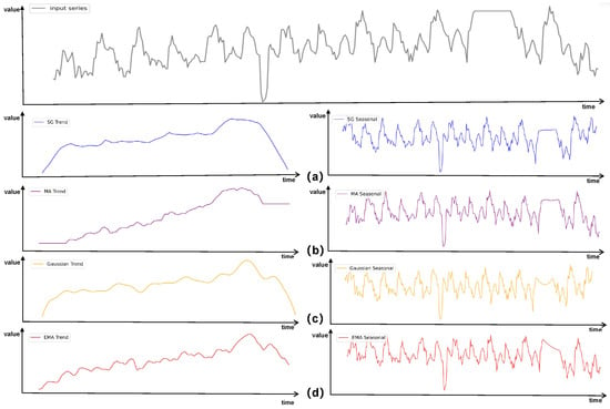
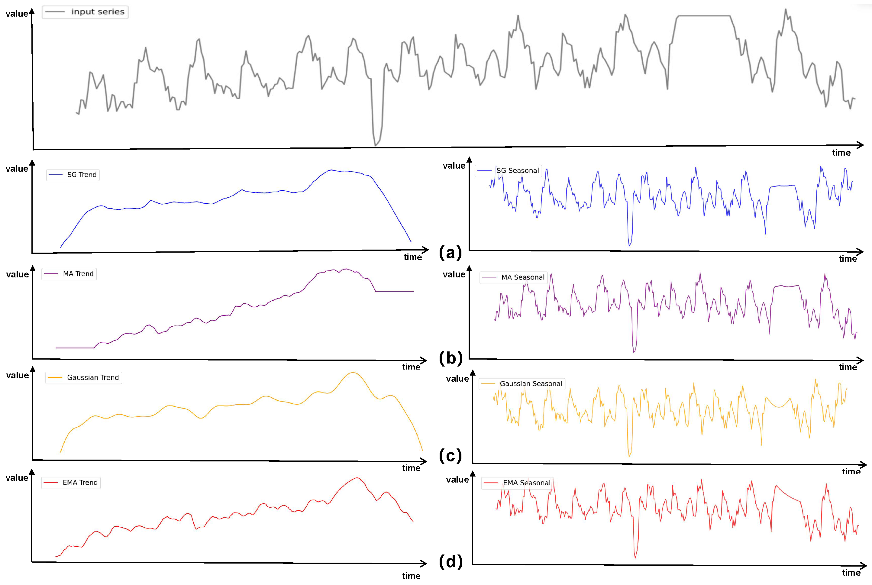
To address this, recent state-of-the-art LTSF models like TimeMixer [17] and xPatch [18] adopt seasonal-trend decomposition to independently capture long-range trends and seasonal variations. The core of this mechanism lies in selecting a smoothing operator to isolate the trend. Historically, these smoothing methods have evolved from the parametric perspective of ARIMA [19] to more flexible localized operators: simple moving averages (e.g., TimeMixer), Gaussian pooling [20], and exponential moving averages (e.g., xPatch). However, these methods share a common structural limitation: they function by redistributing the energy of local sharp peaks along the time axis. In sensor streams with intensive seasonal fluctuations—common when many periodic physical processes are superimposed, as illustrated in Figure 1—this inevitably leads to energy leakage, where multi-scale seasonal features remain residual in the trend component, degrading the fidelity of both the trend and seasonal parts.

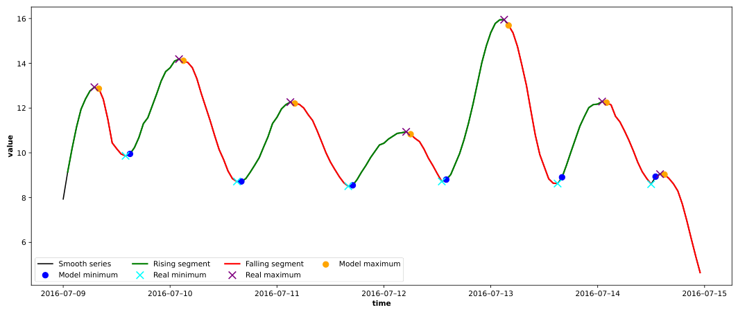
Figure 1. Seasonal-trend decomposition methods. Comparative illustration of SG-Filter-Based Seasonal-Trend Decomposition (a) and other baselines for seasonal-trend decomposition (b–d).

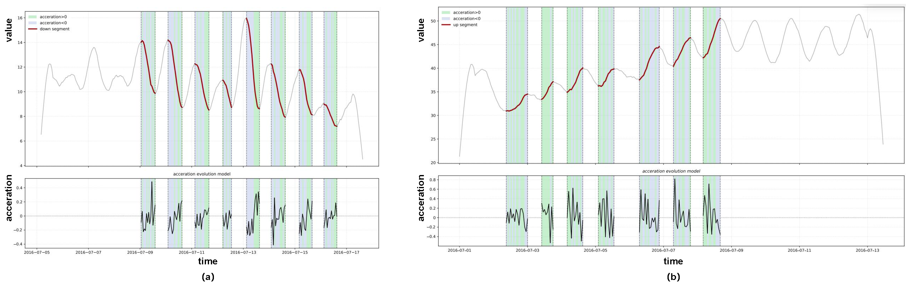
Furthermore, although the seasonal-trend decomposition mechanism improves prediction accuracy, how to perform in-depth feature mining on the extracted trend component remains underexplored. Existing methods represented by Autoformer [21] and FEDformer [22] mainly treat the trend component as a static global description. Specifically, Autoformer isolates the trend through cumulative moving average and utilizes the autocorrelation mechanism for dependency discovery; FEDformer attempts to capture the global contour of the trend by randomly selecting subsets in the frequency domain. However, if the trend is merely regarded as the smooth trajectory produced by low-pass filtering (such as moving average or frequency domain truncation), then these methods mainly focus on the coarse-grained evolution direction (first-order feature $\nabla x$), while ignoring the high-order dynamic information in the trend component. Specifically, they lack effective modeling of the key physical information during the trend evolution (such as curvature or acceleration ${\nabla }^{2}x$). This higher-order information is particularly salient in sensor data, where the underlying processes are physical: as shown in Figure 2, where higher-order acceleration exhibits distinct, recurring pattern features, and the upward segments demonstrate a pronounced driving effect that propels subsequent trend evolutions. This limits the model’s ability to effectively decouple complex non-stationary evolutionary processes and makes it difficult to perceive the sophisticated trend from a deep semantic perspective [23].

Figure 2. Semantic dependencies of sub-trend segments. Correlation analysis of ascending sequences (a) and descending sequences (b).

Accurately modeling local seasonal fluctuation is equally critical in LTSF. To effectively capture multi-scale seasonal fluctuations and overcome the long-term interference caused by global modeling, recent studies have introduced a patch mechanism. These methods are generally classified into two categories: fixed-size patch partitioning such as CARD [14] and PatchTST [12], and multi-/variable-scale partitioning such as TimesNet [9] and Pathformer [24]. In non-stationary sensing environments, particularly under abrupt events such as holiday effects, regime shifts, or sudden sensor excitations, these rigid strategies often lead to the “fragmentation of patterns”, where complete semantic patterns are split across patch boundaries. Meanwhile, to capture the inter-block and intra-block correlations, Pathformer combines the temporal resolution and distance through a dual attention mechanism.

Here, the cross-block attention is used to achieve the overall correlation between blocks; internal block attention handles the local details within them. However, these models tend to over-capture semantically invalid long-range correlations, leading to poor generalization under period drift and an inability to restore continuous semantic coherence across fragmented blocks.

Existing methods address some of these challenges, but none provides a unified solution for accurate decomposition, fine-grained trend modeling, and adaptive patch refactor that is also lightweight enough for embedded deployment. In this paper, we propose the STDPatch framework, which addresses the major limitations in existing LTSF methods. Firstly, we propose a novel decomposition method based on the Savitzky–Golay (SG) Filter [25], which generates a conformal trend component through polynomial fitting, minimizing seasonal noise while preserving the extreme features of the original sequence (as shown in Figure 1a). To address the issue of insufficient depth in trend modeling, we design a new trend decomposition module, explicitly capturing fine-grained phase transformations (rising and falling sub-trends) and high-order physical dynamics. To solve the problem of shape fragmentation and false correlations in seasonal terms, we construct the patch refactor module, adaptively aggregating adjacent patches based on structural similarity, restoring semantic continuity, and filtering out invalid remote interference.

Finally, we introduce a three-stream hybrid architecture in which architectural inductive biases are explicitly matched to the properties of decomposed time series components: CNN for local seasonal regularity, MLP for global trend smoothness, and Transformer for non-stationary sub-trend dynamics. Each branch is designed around well-established efficient building blocks: an activation-free linear backbone, grouped depthwise plus pointwise convolutions, and attention over patch tokens rather than raw time steps. The framework is channel-independent, so the model size is invariant to the number of sensor channels. These design choices position STDPatch as a forecasting backbone suited in principle to sensor-network and edge settings, with on-device deployment left to future work.

The main contributions of this paper are summarized as follows:

• We propose an SG-Filter-based seasonal–trend decomposition method that extracts shape-preserving trends while reducing seasonal leakage.
• We introduce a trend decomposition module that separates trends into ascending and descending segments to capture fine-grained temporal dynamics.
• We develop a patch refactor module that adaptively aggregates neighboring patches based on structural similarity.
• We design a three-stream architecture that combines CNN, MLP, and Transformer branches to model seasonal patterns, global trends, and non-stationary sub-trends.

The remainder of the paper is organized as follows: Section 2 discusses related work. Section 3 presents the proposed framework. Section 4 evaluates our method, and Section 5 concludes this paper.

2. Related Work

2.1. Deep Learning Methods for LTSF

RNNs and their variants (e.g., LSTMs and GRUs [26]) are widely used for sequence modeling, capturing temporal dependencies through hidden states. However, they suffer from the gradient vanishing problem, making it difficult to handle long-term dependencies. LSTMs alleviate this issue via gating mechanisms and memory cells; for instance, Vizi [27] applied it to water level forecasting. Nevertheless, LSTMs still exhibit deficiencies in capturing local trends and rapid fluctuations. Among CNNs, Temporal Convolutional Networks (TCNs) integrate causal convolution, dilated convolution, and residual connections to avoid future information leakage and expand the receptive field, which facilitates the capture of long-term dependencies. The Multi-scale Integrated Convolutional Network (MICN) proposed by Wang [28] can extract both local and global features simultaneously. Yet, TCNs are still constrained by the locality of convolution and struggle to model relationships between distant time points, as noted in ModernTCN [29]. Transformers directly model global dependencies among time points through the self-attention mechanism, achieving strong performance in long-term forecasting. For example, Autoformer [21] and FEDformer [22] optimize seasonal-trend decomposition via self-correlation and frequency-domain attention, respectively. However, the attention mechanism may fail to effectively identify temporal dependencies in complex temporal patterns. As a fundamental architecture, MLPs are also applied to time series forecasting. N-BEATS [30] and LightTS [31] adopt fully connected layers and sampling strategies to achieve efficient forecasting, while NHITS [32] addresses fluctuations and computational issues in long-term forecasting through hierarchical interpolation. Meanwhile, Kolmogorov–Arnold Networks (KANs) replace the fixed linear weights plus activation functions in MLPs with learnable one-dimensional functions, thereby solving the problems of low expression efficiency, severe entanglement of functional structures, and poor interpretability in MLPs [33].

2.2. Evolution of Structural Decoupling in Time Series Forecasting

The evolution of time series forecasting has transitioned from holistic sequence modeling to sophisticated structural decomposition, a trajectory primarily defined by the shift from endogenous integration to explicit decoupling. Early Transformer-based architectures, such as Autoformer [21] and FEDformer [22], pioneered this shift by embedding seasonal-trend decomposition layers directly within neural blocks, utilizing moving average kernels to progressively isolate latent components. While these designs allowed self-attention to operate on stabilized representations, the high computational overhead and potential information leakage in deep-integrated layers led to the rise of explicit structural decoupling. Represented by DLinear [10] and MICN [28], this subsequent paradigm treats decomposition as a fundamental front-end step. DLinear demonstrated that independent linear mappings on decomposed components could effectively mitigate distribution shifts, while MICN introduced multi-scale CNN branches to capture the hierarchical interplay between local morphological fluctuations and global contextual dynamics, offering a more granular perspective on non-stationary series.

Building upon these structural foundations, recent research has focused on the deep fusion of classical statistical priors with modern high-efficiency architectures. Models such as ETSformer [34] and CARD [14] revisit classical state-space principles by integrating exponential smoothing directly into attention mechanisms, thereby enhancing token-level stability. This trend toward refined smoothing has been further extended by TimeMixer [17], which reconciles information across different temporal resolutions via cross-scale decomposition, and xPatch [18], which leverages exponential moving averages (EMAs) within a non-Transformer framework to balance channel independence with patch-wise semantic preservation. Concurrently, recent efforts have also introduced multi-level seasonal-trend decomposition mechanisms [35] to progressively isolate complex, multi-scale non-stationary variations through hierarchical layer structures. Despite these advancements, conventional moving average kernels often suffer from pattern confounding, effectively expanding or shifting temporal energy and sacrificing sharp local phase transitions. Our proposed STDPatch addresses this limitation by deploying a polynomial-fitting SG-Filter for high-fidelity trend extraction, combined with a specialized three-stream parallel architecture to model the decoupled components explicitly. Moreover, by decoupling trends into independent unidirectional processes and employing a similarity-driven patch refactor mechanism, STDPatch achieves a more precise characterization of evolutionary logic while preserving the critical morphological integrity lost in prior methods.

2.3. Block-Based Multivariate Time Series Forecasting

Patch-based strategies have proven highly successful for regularly sampled time series forecasting [12,36,37,38] and have also been extended to irregular multivariate time series forecasting through methods such as tPatchGNN [39] and TimeCHEAT [40]. These studies demonstrate the broad applicability of patch-based representations across different temporal sampling settings. However, many existing approaches still construct patches according to predefined temporal spans or fixed partitioning rules. Although such strategies are simple and computationally efficient, their rigid boundaries may not align with the evolving local structures of non-stationary time series. In particular, a temporally coherent pattern may be divided across adjacent patches when its duration does not match the predefined patch size, while subsequent global modeling may introduce redundant or spurious correlations between structurally dissimilar patches. Adaptive patching methods, such as HDMixer [41], alleviate this limitation by learning more flexible temporal blocks to accommodate varying local dynamics. Nevertheless, preserving structural continuity across neighboring patches while selectively suppressing irrelevant cross-patch interactions remains challenging. To address this issue, we propose a patch refactor mechanism that adaptively aggregates adjacent segments according to structural cosine similarity and learnable hard masks. Rather than changing the original sampling structure, the proposed mechanism operates directly on patch-level semantic representations. Structurally consistent neighboring patches are selectively incorporated into the current representation to restore temporal semantic continuity, whereas dissimilar patches are suppressed to reduce irrelevant interference. In this way, the patch refactor mechanism improves the representation of non-stationary and multi-scale temporal patterns while introducing only limited additional computational overhead.

2.4. Online Learning of Time Series and Streaming Prediction

With the widespread application of sensor technology in real-time monitoring, time series prediction has gradually shifted from the offline batch processing paradigm to the online continuous learning paradigm. Guo et al. [42] initially explored adapting to non-stationary data streams by dynamically updating the weights of neural networks, attempting to capture the evolution of data distribution within limited memory constraints. Recent streaming prediction by Pellicani et al. [43] further emphasizes that in the context of concept drift, the model must possess the ability to adapt immediately, typically adopting memory-based rapid replay mechanisms or lightweight parameter evolution strategies to cope with the continuous input of sensor data.

In the current STDPatch design, we have prioritized addressing the issues of pattern fragmentation and energy leakage in long sequence prediction, ensuring the model’s accuracy advantage when handling complex non-stationary processes. The true online continuous update capability, the immediate reconfiguration of the computational graph, and the automated adaptive autoregressive mechanism for concept drift have been planned as the key focus of our next stage of research. We intend to introduce dynamic memory management and lightweight online fine-tuning strategies in our subsequent work, thereby smoothly transferring the decoupling and representation advantages of STDPatch to the streaming deployment scenarios at the edge.

3. Proposed Method

This section presents the details of STDPatch. Before proceeding, we first give the formal definition of the problem considered. In multivariate time series forecasting, given the observations $x=(x_1,x_2,\dots ,x_L)$ over L historical time steps, the task is to predict the future T time steps $\widehat{x}=(x_{L+1},x_{L+2},\dots ,x_{L+T})$. Each $x_t$ at time step t is multivariate, representing a vector containing M variables. Therefore, the multivariate historical sequence is expressed as $X\in R^{M\times L}$, and the multivariate prediction is expressed as $\widehat{X}\in R^{M\times T}$.

3.1. STDPatch Overview

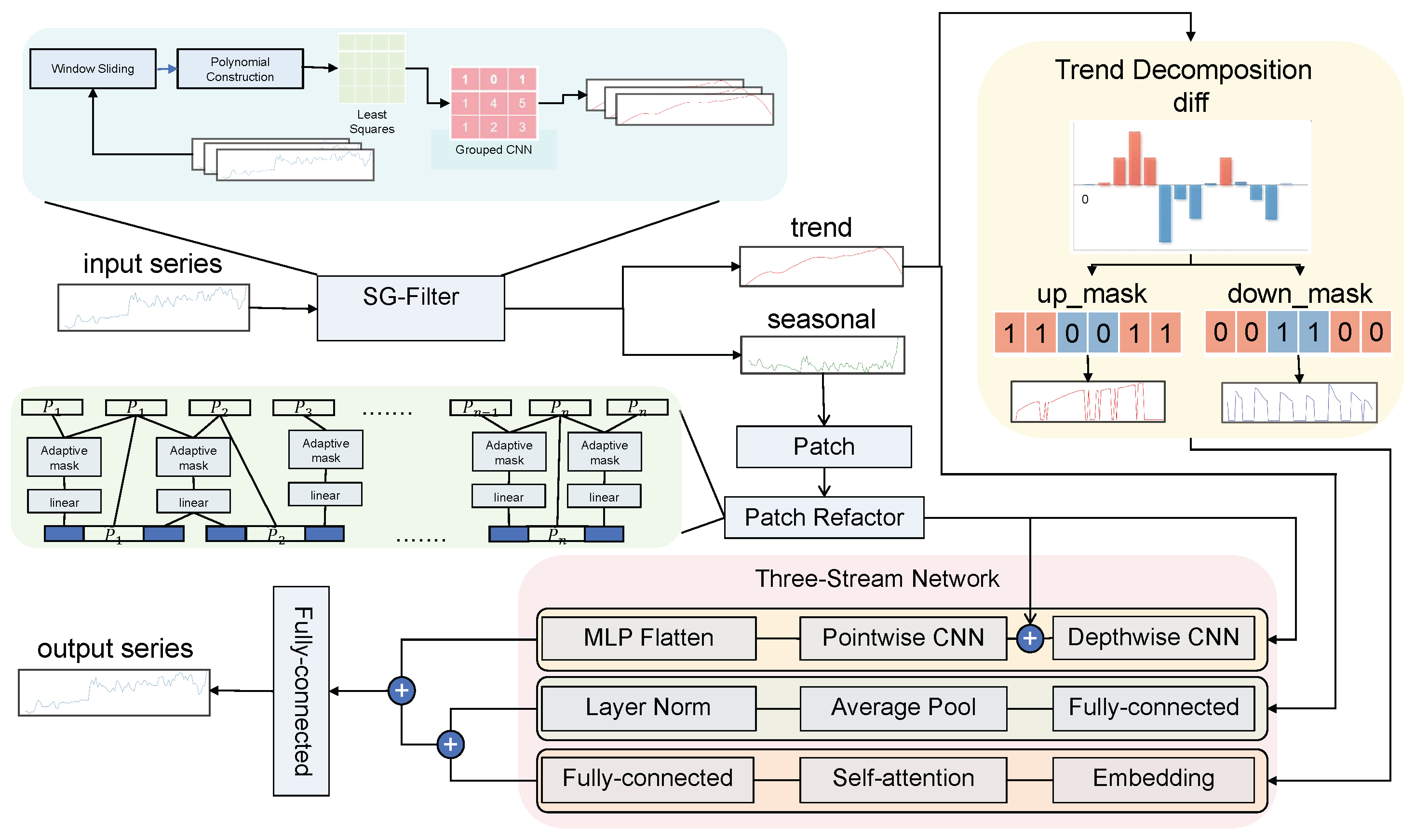
Figure 3 presents the overview of the proposed STDPatch, which consists of four key components:

• The SG-Filter-based Seasonal-Trend Decomposition Module, which achieves a more accurate separation of trend and seasonal components from the original sequence via shape-preserving smoothing technology. It can mitigate the risk of seasonal residuals.
• The Trend Decomposition Module, which further decomposes the trend component of the time series into two key sub-components (ascending and descending components). It enables the model to capture fine-grained dynamic semantics such as acceleration and deceleration within the trend evolution, which are critical for distinguishing different phases of trend development.
• The Patch Refactor Module, which adaptively aggregates adjacent patches to reconstruct the current module through linear projection. It preserves the integrity of local morphological patterns and enhances the consistency of semantic representations across varying temporal scales.
• The Three-Stream Network Architecture, which applies hybrid neural architectures for different decomposed features and achieves more accurate prediction.

Figure 3. Model overview. Each univariate sequence is decomposed by the SG-Filter, and then processed through the three-stream network architecture after undergoing trend decomposition and patch refactor.

Figure 3. Model overview. Each univariate sequence is decomposed by the SG-Filter, and then processed through the three-stream network architecture after undergoing trend decomposition and patch refactor.

3.2. SG-Filter Seasonal-Trend Decomposition Module

Seasonal-trend decomposition facilitates the learning of complex temporal patterns by decomposing time series signals into trend and seasonal components. Trend features typically represent the long-term direction of data, which can be linear or evolve smoothly. In contrast, seasonal components capture recurring patterns or cycles that occur periodically and are usually non-linear due to the complexity and variability of periodic behaviors. The model first learns the features of these components individually and then combines them to generate the final predictions.

Simple Moving Average (SMA) is the decomposition method adopted in Autoformer [21], FEDformer [22], DLinear [10], MICN [28] and TimeMixer [17]. SMA is defined as the unweighted average of k data points. For the moving average point $s_t$ of k entries, where t denotes the moving step, n is the length of the dataset, and $X=\{x_1,x_2,\dots ,x_n\}$ represents the data points, the calculation is as follows:

$$X_T=\mathrm{AvgPool}\left(\mathrm{Padding}\left(X\right)\right).$$

(1)

Gaussian pooling [20] introduces distance weighting to overcome the “one-size-fits-all” problem, with step sizes and kernel sizes predefined through experiments. Its weights are initialized using a Gaussian distribution with the calculation as follows:

$$U[0,0,i]=exp\left(-{\displaystyle \frac{{(i-K/2)}^2}{2{\sigma }^2}}\right),i=1,2,\dots ,K,U\in {\mathbb{R}}^{1\times 1\times K},$$

(2)

$$\omega =\mathrm{Softmax}(U,\dim =-1),$$

(3)

$$X_T=\mathrm{LD}\left(\mathrm{Padding}\left(X_{\mathrm{embed}}\right)\right).$$

(4)

Stitsyuk and Choi argue that the average pooling operation leads to the loss of significant trend features [18]. In addition, alignment requires padding at both ends of the sequence, which may distort the head and tail of the sequence. Therefore, an exponentially weighted scheme, i.e., EMA, is adopted, which can respond more rapidly to changes in the underlying trends of time series without padding repeated values, with the calculation as follows:

$$s_1=x_1,$$

(5)

$$s_t=\alpha x_t+(1-\alpha )s_{t-1},t>0,$$

(6)

$$X_T=\mathrm{EMA}\left(X\right).$$

(7)

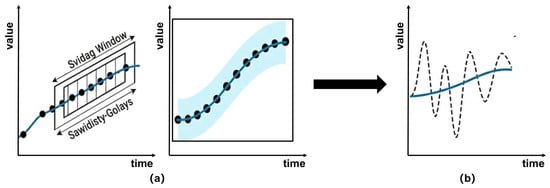
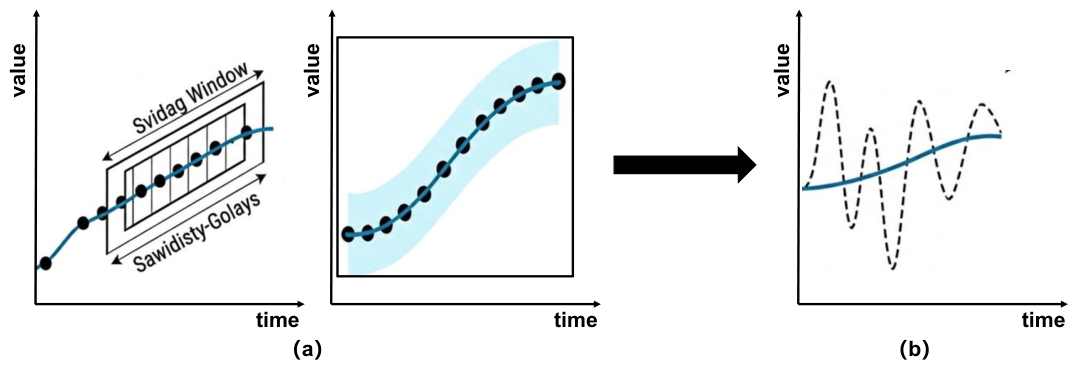
As shown in Figure 4, to extract the trend and seasonal components in time series more accurately, we have designed a novel seasonal-trend decomposition module. Our method uses the SG-Filter to simulate the original sequence by controlling the window size and polynomial order, thus generating a smooth trend curve and minimizing seasonal noise (The settings for the window size and polynomial order of the SG filter can be found in Appendix A). Moreover, most of the seasonal information remaining in the trend term of traditional methods is incorporated into the seasonal term, thereby retaining more complete seasonal information while preserving the overall trend of the original sequence.

$${\widehat{x}}^{\left(d\right)}\left[n\right]={\displaystyle \sum _{k=-M}^M}{c}_k^{\left(d\right)}x[n-k],$$

(8)

where $M={\displaystyle \frac{W-1}{2}}$, $c_k^{\left(d\right)}$ denotes the SG coefficient corresponding to the d-th order derivative (w and $win\_length$ are the input window lengths of the SG-Filter); when $d=0$, it corresponds to smooth filtering; when $d>0$, it corresponds to derivative approximation. The convolution kernel ${\mathbf{c}}^{\left(d\right)}$ is derived from the design of the Savitzky–Golay filter:

$${\mathit{c}}_d={\mathit{e}}_d^{\mathrm{T}}{\mathit{A}}^{\mathrm{T}}{\mathit{A}}^{-1}{\mathit{A}}^{\mathrm{T}},$$

(9)

where A represents the polynomial basis matrix (each column is $1,n,n^2,\dots$), ${\mathbf{e}}_d$: the unit vector for selecting the d-th order derivative.

$$X_T=\mathrm{SG}\left(X\right),$$

(10)

$$X_S=X-X_T,$$

(11)

Figure 4. Signal processing workflow based on SG convolution smoothing: (a) algorithm principle example and (b) operator engineering example.

Equations (10) and (11) formalize the decomposition process: the SG-Filter first extracts a shape-preserving trend $X_T$ from the original sequence X; the seasonal component $X_S$ is then obtained as the residual $X-X_T$, isolating periodic fluctuations from the long-term evolution.

3.3. Trend Decomposition Module

We further decompose the trend component of the time series into two critical sub-components: an upward segment and a downward segment. These two segments alternate and connect with each other, jointly forming a complete trend trajectory. This decomposition method aims to extract more fine-grained unidirectional movement patterns from the macro trend, thereby characterizing the long-term evolutionary features of the series more accurately. The trend component is processed with linear blocks to capture the slowly varying long-term constituents in the series; in contrast, the upward segment and downward segment are modeled using Transformer blocks. This is because these segments represent complex, dynamic nonlinear variation patterns in the series, and the Transformer can more effectively capture these local and non-stationary dependencies by virtue of its powerful attention mechanism [44]. Our trend decomposition algorithm generates upward and downward masks by calculating the differences between adjacent time steps in the time series data.

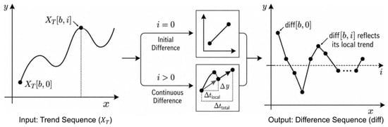
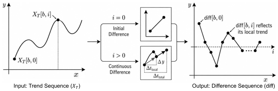
The differential operation characterizes the variation trend of the time series at adjacent positions, as shown in Figure 5. For the first time step $i=0$, since there is no preceding time step, the original value $X_{\mathrm{T}}[b,0]$ is directly used as the initial difference value; for subsequent time steps, the local variation is obtained by computing the difference between the current and the preceding time step. This differential operation can explicitly reflect the upward or downward trend of the series, providing a basis for the subsequent construction of directional masks. The calculation process of diff is as follows:

$$\mathrm{diff}[b,i]=\left\{\begin{array}{cc}{X}_T[b,0],\hfill & i=0\hfill \\ X_T[b,i]-X_T[b,i-1],\hfill & i=1,\dots ,L-1\hfill \end{array}\right..$$

(12)

Figure 5. The calculation workflow of the difference sequence.

Based on the differencing results, we construct an upward mask ($\mathrm{up}\_\mathrm{mask}$) and a downward mask ($\mathrm{down}\_\mathrm{mask}$), respectively. If the difference is positive, it indicates an upward trend compared to the previous time step, and the $\mathrm{up}\_\mathrm{mask}$ is set to 1. Conversely, when the difference is less than or equal to 0, the sequence is in a downward or stable state, and the $\mathrm{down}\_\mathrm{mask}$ is set to 1:

$$\mathrm{up}\_\mathrm{mask}[b,i]=\left\{\begin{array}{c}1,\mathrm{diff}[b,i]\ge 0\hfill \\ 0,\mathrm{otherwise}\hfill \end{array}\right.\hspace{1em},\mathrm{down}\_\mathrm{mask}[b,i]=\left\{\begin{array}{c}1,\mathrm{diff}[b,i]<0\hfill \\ 0,\mathrm{otherwise}\hfill \end{array}\right.\hspace{1em}.$$

(13)

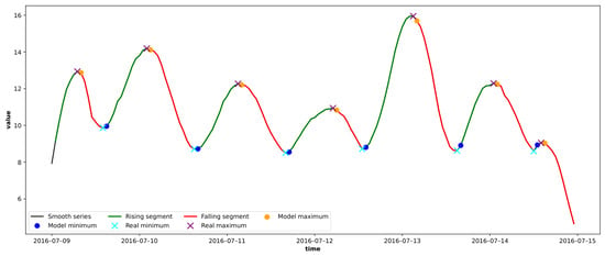
This design discretizes continuous numerical changes into explicit directional trends through simple sign determination. To intuitively verify the effectiveness of this mechanism, the internally generated masks are compared with the local extrema of the original sequence, as illustrated in Figure 6. The visualization demonstrates that the switching points of the masks align closely with the peaks and troughs of the original data. This confirms that the model accurately captures critical trend turning points, providing reliable directional guidance for the subsequent trend decomposition stream.

Figure 6. Comparison of local extrema between the masked sequence and the original sequence.

After obtaining the masks, they are multiplied with the original feature sequence to generate new sequences: the upward sequence retains the original features only at upward time steps, with all other positions set to zero; the downward sequence retains features only at downward or stationary time steps. In this way, the original sequence is split into two sub-sequences distinguished by their variation directions:

$$\begin{array}{c}\hfill T_{\mathrm{up}}[b,i,:]=\mathrm{up}\_\mathrm{mask}[b,i]t[b,i,:],T_{\mathrm{down}}[b,i,:]=\mathrm{down}\_\mathrm{mask}[b,i]t[b,i,:].\end{array}$$

(14)

By modeling the decoupled sub-trends $T_{\mathrm{up}}$ and $T_{\mathrm{down}}$ via Transformer blocks rather than conventional first-order smoothing operators, the framework effectively captures complex, non-linear dependencies. Formally, the feature extraction on each sub-trend can be compactly represented as:

$$H_{\psi }=A_{\psi }{\mathbf{V}}_{\psi },\psi \in \{\mathrm{up},\mathrm{down}\},$$

(15)

where $A_{\psi }$ denotes the temporal affinity (attention) matrix generated within the Transformer block. Crucially, $A_{\psi }$ functions as an implicit, data-driven differential operator. Since its elements $A_{\psi }[i,j]$ quantify the transitional momentum and dynamic rates of change between directional states at time segments i and j, this design empowers STDPatch to capture high-order physical dynamics such as curvature and acceleration (${\nabla }^{2}x$). Consequently, the model accurately perceives sophisticated trend transitions and structural regime shifts to guide long-term forecasting.

3.4. Patch Refactor Module

Traditional patch partitioning methods based on fixed lengths and intervals are simple to implement and computationally efficient, yet their rigid structures struggle to adapt to the dynamic variation characteristics of different periodic and trend components in time series. This one-size-fits-all partitioning approach has three limitations:

• It tends to split integral morphological features (e.g., complete cycles of public opinion or economic fluctuations), disrupting inherent semantic continuity [24].
• Insufficient overlap between segments risks losing transitional information, while excessive overlap causes feature redundancy and computational overhead [12].
• It fails to adapt to multi-scale characteristics, making it unable to capture both short-term fluctuations and long-term trends simultaneously.

These limitations severely restrict the model’s expressive capacity for complex time series patterns, especially when processing data with irregular periodicity and abrupt fluctuation characteristics.

To calculate the local similarity later, we have divided the continuous time series into non-overlapping patches:

$${\mathit{s}}_{p,k}^{\left(i\right)}=\mathrm{unfold}\left(\mathit{s},\mathrm{dimension}=-1,\mathrm{size}=P,\mathrm{step}=P\right),$$

(16)

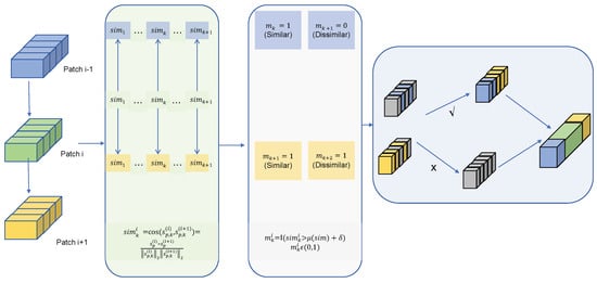
where i represents the i-th patch, and $k\in \{1,\dots ,B\times C\}$ represents a composite index that simultaneously covers the batch size B and the channel dimension C. Compared with the fixed partitioning strategy (as shown in Figure 7), we propose a dynamically adaptive patch refactor mechanism based on the similarity of adjacent patches, which performs fine-grained modeling of temporal structures via a learnable hard mask. Specifically, the model first calculates the cosine similarity between the representations of adjacent patches, takes the sample-level statistical mean as the benchmark, and introduces a learnable bias to adaptively determine the similarity threshold, thereby generating a binary mask that characterizes whether adjacent patches should be regarded as the same semantic structure. The process of constructing similarity is as follows:

$${\mathrm{sim}}_k^{\left(i\right)}=cos\left({\mathit{s}}_{p,k}^{\left(i\right)},{\mathit{s}}_{p,k}^{(i+1)}\right)={\displaystyle \frac{{\mathit{s}}_{p,k}^{\left(i\right)}·{\mathit{s}}_{p,k}^{(i+1)}}{{∥{\mathit{s}}_{p,k}^{\left(i\right)}∥}_2{∥{\mathit{s}}_{p,k}^{(i+1)}∥}_2}}.$$

(17)

Figure 7. Patch Refactor via semantic correlation analysis.

Building on this foundation, we reconstruct patches in both forward and backward directions, respectively: for adjacent patches with similarity above the threshold, their features are retained and aggregated into the current patch; for patches with low similarity, their contributions are directly suppressed, thus avoiding the interference of structurally discontinuous or semantically irrelevant segments with the current representation. This selective aggregation mechanism based on hard masks enables the model to effectively reduce the introduction of redundant information while preserving structural discriminability.

$$m_k^{\left(i\right)}=\mathrm{I}\left({\mathrm{sim}}_k^{\left(i\right)}\ge \mu \left(\mathrm{sim}\right)+\delta \right),m_k^{\left(i\right)}\in \{0,1\},$$

(18)

where $\delta$ is a hyperparameter that controls the strictness of the binarization process. Guided by the hard masks $m_k^{(i-1)}$ and $m_k^{\left(i\right)}$, the model selectively propagates contextual information from the previous and subsequent patches via learnable linear projections ($W_{\mathrm{prev}},b_{\mathrm{prev}}$ and $W_{\mathrm{next}},b_{\mathrm{next}}$) to enrich the current representation ${\tilde{\mathit{s}}}_{p,k}^{(i+1)}$, effectively forming longer valid macro-evolution segments in stable regions while fully suppressing noise interference from structurally discontinuous segments:

$${\tilde{\mathit{s}}}_{p,k}^{(i+1)}={\mathit{s}}_{p,k}^{(i+1)}+m_k^{(i-1)}·\left(W_{\mathrm{prev}}{\mathit{s}}_{p,k}^{(i-1)}+b_{\mathrm{prev}}\right)+m_k^{\left(i\right)}·\left(W_{\mathrm{next}}{\mathit{s}}_{p,k}^{(i+1)}+b_{\mathrm{next}}\right).$$

(19)

This mechanism offers three advantages:

• The structural similarity-based hard mask strategy preserves critical morphological structures (e.g., complete periodic fluctuations) within individual patches and reinforces local semantic consistency.
• The adaptive patch aggregation method inherently supports multi-scale modeling, enabling the unified characterization of short-term fluctuations and long-term trends.
• The reconstruction process based on binary masks incurs extremely low computational overhead, maintaining high overall computational efficiency while improving representation quality.

3.5. Three-Stream Network Architecture

Refined seasonal-trend pre-decomposition is achieved via the SG-Filter in STDPatch, where a “three-stream parallel” architecture is used to tackle the complex non-stationary evolution inherent in real-world time series. The core value of this architecture lies in its superior feature decoupling capability: the seasonal convolutional stream leverages local receptive fields to capture high-frequency periodic patterns; the trend linear stream anchors global evolutionary inertia through comprehensive mapping; and the trend decomposition Transformer stream specifically addresses “intermittent” non-linear jumps and long-range dependencies within trends. This approach effectively resolves the pattern confusion issues typical of traditional single-stream models when processing trend shifts. Although the three-stream design introduces certain overhead in parallel computing and memory synchronization, when coupled with patch refactor technology, the model can synergize semantic information across multiple scales. This design—trading moderate computational redundancy for specialized stream processing—significantly enhances the precision in capturing state transitions within non-stationary systems (To assess our consumption, we also conducted certain experiments, as can be seen in the Appendix A), providing a robust deep learning paradigm with solid physical–logical grounding for complex time series forecasting.

Linear Stream: The linear stream is an MLP-based network that includes average pooling and layer normalization, with the activation function omitted to emphasize linear features.

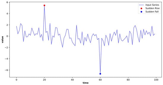
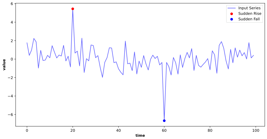
The decomposed data $x^{\left(i\right)}$ is passed through two linear blocks, each consisting of a fully connected layer. To address the abrupt noise points present in the trend component (as shown in Figure 8), we adopt average pooling with a kernel size of k = 2 for feature smoothing, along with layer normalization to ensure training stability. Each linear layer and average pooling operation contributes to dimensionality reduction, encouraging the network to compress feature representations for efficient adaptation to the available space. This reduction in the number of features, combined with the absence of activation functions and bottleneck architectures, is designed to retain only the most important linear features of the smooth trend:

$$X_T^{\left(l\right)}=\mathrm{LayerNorm}\left(\mathrm{AvgPool}\left(\mathrm{Linear}\left(X_T^{\left(l\right)}\right),k=2\right)\right).$$

(20)

Figure 8. Intuitively displayed time slices, surge noise points and drop noise points.

Transformer Stream: The ascending and descending sequences derived from trend decomposition are used to project the input queries (Q), keys (K), and values (V) into multiple head spaces via linear transformations. We then calculate the scaled dot-product attention scores, apply softmax and dropout to obtain the attention weights, and generate the contextual representations through a weighted sum of the weights and values. Finally, the output is obtained via an output linear layer, residual connection, and layer normalization, with the averaged attention weights returned simultaneously for visual analysis:

$$\mathrm{Attention}\left({\mathcal{T}}_i\right)=\mathrm{softmax}\left({\displaystyle \frac{Q_{i+1}{K}_{i+1}^{\mathrm{T}}}{\sqrt{d_k}}}\right)\ast V_{i+1},$$

(21)

$$Q_{i+1}=f_1\left({\mathcal{T}}_i\right),K_{i+1}=f_2\left({\mathcal{T}}_i\right),V_{i+1}=f_3\left({\mathcal{T}}_i\right).$$

(22)

The core function of the embedding layer (typically realized by segmenting a sequence into sub-sequential patches and performing linear projection) is to convert the single-channel value of each time step into a semantic vector representation that can characterize its local temporal context. Instead of mapping words to a vector space, it maps a short time sequence segment to a temporal semantic vector. In this way, the original scalar time series points are lifted to a vector space rich in local trend and morphological information, enabling the subsequent Transformer-based self-attention mechanism to effectively capture and measure the long-range dependencies and pattern similarities between these temporal semantic vectors in the same way it processes natural language:

$${\mathbf{E}}_{b,t,j}={\displaystyle \sum _{c=1}^C}{T}_{b,t,c}·W_{c,j}+b_j,$$

(23)

$${\mathbf{E}}_{b,t,j}={\displaystyle \sum _{c=1}^C}\left(\sum _k{T}_{b,t,c}·V_{c,j,k}+u_{j,k}\right),$$

(24)

For a small or moderate number of channels (C < 100), Scheme 2 (Summing after independent embedding) has sufficient computational resources and data to support the model in learning complex channel interactions while mitigating overfitting risks. This scheme preserves more fine-grained details and offers greater modeling potential.

For an extremely large number of channels (C > 100), Scheme 1 (Direct joint embedding) forces the model to retain only the most important cross-channel collaborative signals while ignoring a large number of insignificant or redundant channel details. This greatly reduces the model’s degrees of freedom, driving it to learn highly generalizable and robust feature representations, thereby alleviating overfitting.

Convolution Stream: The embedded and repaired data $X_p^{\left(i\right)}\in {\mathbb{X}}^{N\times P}$ is processed to increase the number of features via the activation function $\sigma$ and batch normalization. This is intended to capture comprehensive semantic information that may not be attainable at the point level and to enable the focus on non-linear features. For deepwise convolution, we adopt grouped convolution, where the number of groups g is equal to the number of patches N, the large kernel size k is equal to the patch length P, and the convolution stride s is equal to the patch length P:

$$S_p^{N\times P}={\mathrm{Conv}}_{N\to N}\left(S_p^{N\times P^2},k=P,s=P,g=N\right)$$

(25)

Information fusion and feature transformation among variables are then performed via a $1\times 1$ pointwise convolution (Pointwise Conv), followed by non-linear transformation through batch normalization (BatchNorm) and an activation function. This structure significantly reduces the number of computational parameters while preserving the model’s expressive capacity:

$$S_p^{N\times P}=\mathrm{DepthwiseConv}\left(S_p^{N\times P^2}+S_p^{N\times P^2}\right),$$

(26)

$$S_p^{N\times P}={\mathrm{Conv}}_{N\to N}\left(S_p^{N\times P},k=1,s=1,g=1\right).$$

(27)

3.6. Final Prediction

The final prediction module integrates the outputs from three parallel training branches: the Transformer branch, the CNN branch, and the MLP branch. By aggregating the features captured by different architectures, the model generates the final prediction result. The aggregation process is formulated as follows:

$$X_{\mathrm{trans}}=\mathrm{Transformer}\left(X_{\mathrm{up}}\right)+\mathrm{Transformer}\left(X_{\mathrm{down}}\right),$$

(28)

$$\widehat{Y}=\mathrm{FC}\left(X_{\mathrm{trans}}+\mathrm{MLP}\left(X_T\right)+\mathrm{CNN}\left(X_S\right)\right)$$

(29)

To maintain consistency with the dimensions of the ground truth, the aggregated patch features are projected and reshaped through a fully connected layer (FC). The final output is converted to $\widehat{Y}\in {\mathbb{R}}^{M\times T}$.

4. Experiments

4.1. Experimental Settings

Datasets: We conduct extensive experiments on seven real-world multivariate time series datasets, including Electricity Transformer Temperature (ETTh1, ETTh2, ETTm1, ETTm2), Weather, Traffic, and Electricity.

Evaluation Metrics: Following previous work, we use Mean Squared Error (MSE) and Mean Absolute Error (MAE) metrics to evaluate performance.

Implementation Details: All experiments are implemented in PyTorch 2.7.0 [45] and conducted on a single Nvidia RTX 4090 GPU.

Baselines: We select the latest LTSF models as the baselines for our experiments, including TimeKAN (2025), xPatch (2025), TimeMixer (2024), iTransformer (2024), MSGNet (2024), TimesNet (2023), MICN (2023), DLinear (2023), PatchTST (2023). All implementations are derived from the official repository code of the models with the same configurations retained. It is also worth noting that we strictly adhere to the settings specified in the official implementations, including the number of training epochs and the learning rate adjustment strategy.

Unified Experimental setting: To ensure a fair comparison, we perform two types of experiments. For all other datasets, the first experiment adopts a unified setting based on the prediction protocol proposed by TimesNet (2023), with $L=96$ and $T=\{96,192,336,720\}$. The experimental results are reported in Table 1.

Table 1. For all datasets, a unified lookback window of $L=96$ is adopted. All results are derived from four distinct prediction horizons with their average value, denoted as $T=\{96,192,336,720,\mathrm{avg}\}$. The best-performing model is displayed in red font, and the second-best model in blue font.

Dataset	Horizon	STDPatch		TimeKAN		xPatch		TimeMixer		iTransformer		MSGNet		TimesNet		MICN		DLinear		PatchTST
		MSE	MAE	MSE	MAE	MSE	MAE	MSE	MAE	MSE	MAE	MSE	MAE	MSE	MAE	MSE	MAE	MSE	MAE	MSE	MAE
ETTh1	96	0.364	0.385	0.367	0.395	0.376	0.386	0.385	0.402	0.386	0.405	0.390	0.411	0.384	0.402	0.426	0.446	0.397	0.412	0.393	0.407
	192	0.401	0.404	0.414	0.420	0.417	0.407	0.443	0.430	0.441	0.436	0.422	0.442	0.436	0.429	0.454	0.464	0.446	0.441	0.445	0.434
	336	0.423	0.421	0.445	0.434	0.449	0.425	0.512	0.470	0.487	0.458	0.480	0.468	0.638	0.469	0.493	0.487	0.489	0.467	0.483	0.451
	720	0.439	0.446	0.444	0.459	0.470	0.456	0.497	0.476	0.503	0.491	0.494	0.488	0.521	0.500	0.526	0.526	0.513	0.510	0.479	0.470
	Avg	0.406	0.414	0.417	0.427	0.428	0.419	0.459	0.444	0.454	0.448	0.446	0.452	0.495	0.450	0.475	0.480	0.461	0.457	0.450	0.441
ETTh2	96	0.231	0.299	0.290	0.340	0.233	0.300	0.289	0.342	0.297	0.349	0.328	0.371	0.340	0.374	0.372	0.424	0.340	0.394	0.293	0.342
	192	0.287	0.336	0.375	0.392	0.291	0.338	0.378	0.397	0.380	0.400	0.402	0.414	0.402	0.414	0.492	0.492	0.482	0.479	0.377	0.393
	336	0.336	0.374	0.423	0.435	0.344	0.377	0.432	0.434	0.428	0.432	0.435	0.443	0.452	0.452	0.607	0.555	0.591	0.541	0.380	0.408
	720	0.401	0.425	0.443	0.449	0.407	0.427	0.464	0.464	0.427	0.445	0.417	0.441	0.462	0.468	0.824	0.655	0.839	0.661	0.411	0.433
	Avg	0.313	0.359	0.383	0.404	0.319	0.361	0.390	0.409	0.383	0.407	0.395	0.417	0.414	0.427	0.574	0.531	0.563	0.519	0.365	0.394
ETTm1	96	0.307	0.336	0.322	0.361	0.311	0.346	0.317	0.356	0.334	0.368	0.319	0.366	0.338	0.375	0.365	0.387	0.346	0.374	0.320	0.359
	192	0.348	0.370	0.357	0.383	0.348	0.368	0.367	0.384	0.377	0.391	0.376	0.397	0.374	0.387	0.403	0.408	0.382	0.391	0.365	0.381
	336	0.381	0.388	0.382	0.401	0.388	0.391	0.391	0.406	0.426	0.420	0.417	0.422	0.410	0.411	0.436	0.431	0.415	0.415	0.391	0.401
	720	0.456	0.429	0.445	0.435	0.461	0.430	0.454	0.441	0.491	0.459	0.481	0.458	0.478	0.450	0.489	0.462	0.473	0.451	0.455	0.436
	Avg	0.373	0.380	0.376	0.395	0.377	0.384	0.382	0.397	0.407	0.410	0.398	0.410	0.400	0.406	0.423	0.422	0.404	0.408	0.383	0.394
ETTm2	96	0.151	0.238	0.174	0.255	0.164	0.248	0.175	0.257	0.180	0.264	0.177	0.262	0.187	0.267	0.197	0.296	0.193	0.293	0.177	0.259
	192	0.205	0.275	0.239	0.299	0.230	0.291	0.240	0.302	0.250	0.309	0.247	0.307	0.249	0.309	0.284	0.361	0.284	0.361	0.248	0.306
	336	0.252	0.307	0.301	0.340	0.292	0.331	0.303	0.343	0.311	0.348	0.312	0.346	0.321	0.351	0.381	0.429	0.382	0.429	0.313	0.346
	720	0.318	0.349	0.395	0.396	0.381	0.383	0.392	0.396	0.412	0.407	0.414	0.403	0.408	0.403	0.549	0.522	0.558	0.525	0.399	0.397
	Avg	0.231	0.292	0.277	0.322	0.267	0.313	0.277	0.324	0.288	0.332	0.287	0.329	0.291	0.333	0.353	0.402	0.354	0.402	0.284	0.327
Weather	96	0.161	0.197	0.162	0.208	0.168	0.203	0.163	0.209	0.174	0.214	0.163	0.212	0.172	0.220	0.198	0.261	0.195	0.252	0.177	0.218
	192	0.206	0.240	0.207	0.249	0.214	0.245	0.211	0.254	0.221	0.254	0.212	0.254	0.219	0.261	0.239	0.299	0.237	0.295	0.225	0.259
	336	0.239	0.273	0.263	0.290	0.236	0.273	0.263	0.293	0.278	0.296	0.272	0.299	0.246	0.337	0.285	0.336	0.282	0.331	0.277	0.297
	720	0.317	0.327	0.338	0.340	0.309	0.321	0.344	0.348	0.358	0.347	0.350	0.348	0.365	0.359	0.351	0.388	0.345	0.382	0.350	0.345
	Avg	0.230	0.259	0.242	0.272	0.232	0.261	0.245	0.276	0.258	0.278	0.249	0.278	0.251	0.294	0.268	0.321	0.265	0.315	0.257	0.280
Electricity	96	0.149	0.241	0.174	0.266	0.159	0.244	0.153	0.245	0.148	0.240	0.165	0.274	0.168	0.272	0.180	0.293	0.210	0.302	0.166	0.252
	192	0.159	0.251	0.182	0.273	0.160	0.248	0.166	0.257	0.162	0.253	0.184	0.292	0.184	0.322	0.189	0.302	0.210	0.305	0.173	0.260
	336	0.181	0.272	0.197	0.286	0.182	0.267	0.185	0.275	0.178	0.269	0.195	0.302	0.198	0.300	0.198	0.312	0.223	0.319	0.190	0.277
	720	0.213	0.298	0.236	0.320	0.216	0.298	0.224	0.312	0.225	0.317	0.231	0.332	0.220	0.320	0.217	0.330	0.258	0.350	0.230	0.311
	Avg	0.175	0.265	0.197	0.286	0.179	0.264	0.182	0.272	0.178	0.270	0.193	0.300	0.193	0.304	0.196	0.309	0.225	0.319	0.190	0.275
Traffic	96	0.472	0.283	0.612	0.383	0.471	0.275	0.462	0.285	0.395	0.268	0.511	0.300	0.593	0.321	0.519	0.309	0.650	0.396	0.446	0.283
	192	0.474	0.286	0.574	0.365	0.478	0.272	0.473	0.296	0.417	0.276	0.538	0.311	0.617	0.336	0.537	0.315	0.598	0.370	0.453	0.285
	336	0.489	0.292	0.561	0.365	0.501	0.276	0.498	0.296	0.433	0.283	0.562	0.322	0.629	0.336	0.534	0.313	0.605	0.373	0.467	0.291
	720	0.522	0.307	0.614	0.383	0.547	0.291	0.506	0.313	0.467	0.302	0.591	0.338	0.640	0.350	0.577	0.325	0.645	0.394	0.500	0.309
	Avg	0.489	0.292	0.590	0.374	0.499	0.279	0.484	0.298	0.428	0.282	0.550	0.317	0.620	0.336	0.541	0.315	0.625	0.383	0.467	0.292
1st Count		25/24		1/0		3/11		0/0		7/2		0/0		0/0		0/0		0/0		0/0

Hyperparameter Search: Due to the high computational cost of the transformer stream, we replace it with the linear stream during hyperparameter search. After identifying the optimal hyperparameters, the transformer stream is restored, and all final experiments are conducted using the optimized configuration. In the second experiment, our goal is to determine the upper bound of the compared models and conduct a hyperparameter search. We evaluate all models to check whether they benefit from longer historical data, so as to identify the optimal lookback length for each model. A hyperparameter search is performed for models benefiting from longer input lengths, including TVNet (2025) [46], TimeMixer (2024), iTransformer (2024), TimesNet (2023), MICN (2023), DLinear (2023), and PatchTST (2023), following the methodology established in TimeMixer (2024). The experimental results are shown in Table 2.

Table 2. For all datasets, all results are obtained for four distinct prediction horizons along with their average value, denoted as $T=\{96,192,336,720,\mathrm{avg}\}$. The best-performing model is displayed in red font, and the second-best one in blue font.

Dataset	Horizon	STDPatch		TVNet		TimeMixer		iTransformer		TimesNet		MICN		DLinear		PatchTST
		MSE	MAE	MSE	MAE	MSE	MAE	MSE	MAE	MSE	MAE	MSE	MAE	MSE	MAE	MSE	MAE
ETTh1	96	0.350	0.389	0.371	0.408	0.361	0.390	0.396	0.425	0.384	0.402	0.398	0.427	0.375	0.399	0.370	0.400
	192	0.374	0.408	0.398	0.409	0.409	0.414	0.430	0.450	0.436	0.429	0.430	0.453	0.405	0.416	0.413	0.429
	336	0.391	0.418	0.401	0.409	0.430	0.429	0.479	0.485	0.491	0.469	0.440	0.460	0.439	0.443	0.422	0.440
	720	0.431	0.455	0.458	0.459	0.445	0.460	0.700	0.608	0.521	0.500	0.491	0.509	0.472	0.490	0.447	0.468
	Avg	0.386	0.417	0.407	0.421	0.411	0.423	0.501	0.492	0.458	0.450	0.440	0.462	0.423	0.437	0.413	0.434
ETTh2	96	0.232	0.308	0.263	0.329	0.271	0.330	0.311	0.363	0.340	0.374	0.299	0.364	0.289	0.353	0.274	0.337
	192	0.270	0.340	0.319	0.372	0.317	0.402	0.391	0.413	0.402	0.414	0.422	0.441	0.383	0.418	0.341	0.382
	336	0.315	0.379	0.311	0.373	0.332	0.396	0.415	0.437	0.452	0.452	0.447	0.474	0.448	0.465	0.329	0.384
	720	0.389	0.425	0.401	0.434	0.342	0.408	0.424	0.455	0.462	0.468	0.442	0.467	0.605	0.551	0.379	0.422
	Avg	0.301	0.363	0.324	0.377	0.316	0.384	0.385	0.417	0.414	0.427	0.403	0.437	0.431	0.447	0.331	0.381
ETTm1	96	0.288	0.341	0.288	0.343	0.291	0.340	0.313	0.366	0.338	0.375	0.316	0.364	0.299	0.343	0.293	0.346
	192	0.325	0.364	0.326	0.367	0.327	0.365	0.349	0.388	0.374	0.387	0.363	0.390	0.335	0.365	0.333	0.370
	336	0.354	0.381	0.365	0.391	0.360	0.381	0.381	0.411	0.410	0.411	0.408	0.426	0.369	0.386	0.369	0.392
	720	0.400	0.406	0.412	0.413	0.415	0.417	0.448	0.449	0.478	0.450	0.459	0.464	0.425	0.421	0.416	0.420
	Avg	0.341	0.373	0.348	0.379	0.348	0.376	0.373	0.404	0.400	0.406	0.387	0.411	0.357	0.379	0.353	0.382
ETTm2	96	0.154	0.246	0.161	0.254	0.164	0.254	0.180	0.274	0.187	0.267	0.179	0.275	0.167	0.260	0.166	0.256
	192	0.188	0.270	0.220	0.293	0.223	0.295	0.238	0.311	0.249	0.309	0.262	0.326	0.224	0.303	0.223	0.296
	336	0.230	0.295	0.272	0.316	0.279	0.330	0.294	0.349	0.321	0.351	0.305	0.353	0.281	0.342	0.274	0.329
	720	0.285	0.340	0.349	0.379	0.359	0.383	0.382	0.406	0.408	0.403	0.389	0.407	0.397	0.421	0.362	0.385
	Avg	0.214	0.287	0.251	0.311	0.256	0.316	0.274	0.335	0.291	0.333	0.284	0.340	0.267	0.332	0.256	0.317
Weather	96	0.144	0.183	0.147	0.198	0.147	0.197	0.191	0.239	0.172	0.220	0.161	0.229	0.176	0.237	0.149	0.198
	192	0.188	0.227	0.194	0.238	0.189	0.239	0.219	0.263	0.219	0.261	0.220	0.281	0.220	0.282	0.194	0.241
	336	0.224	0.264	0.235	0.277	0.241	0.280	0.284	0.311	0.280	0.306	0.278	0.331	0.265	0.319	0.245	0.282
	720	0.291	0.317	0.308	0.331	0.310	0.330	0.389	0.375	0.365	0.359	0.311	0.356	0.323	0.362	0.314	0.334
	Avg	0.211	0.248	0.221	0.261	0.222	0.262	0.271	0.297	0.259	0.287	0.243	0.299	0.246	0.300	0.226	0.264
Electricity	96	0.127	0.220	0.142	0.223	0.129	0.224	0.131	0.227	0.168	0.272	0.164	0.269	0.140	0.237	0.129	0.222
	192	0.144	0.235	0.165	0.241	0.140	0.220	0.152	0.248	0.184	0.289	0.177	0.285	0.153	0.249	0.147	0.240
	336	0.160	0.252	0.164	0.269	0.161	0.255	0.170	0.267	0.198	0.300	0.193	0.304	0.169	0.267	0.163	0.259
	720	0.200	0.288	0.190	0.284	0.194	0.287	0.190	0.284	0.220	0.320	0.212	0.321	0.203	0.301	0.197	0.290
	Avg	0.157	0.248	0.165	0.254	0.156	0.247	0.161	0.257	0.193	0.295	0.187	0.295	0.166	0.264	0.159	0.253
Traffic	96	0.378	0.250	0.367	0.252	0.360	0.249	0.348	0.255	0.593	0.321	0.519	0.309	0.410	0.282	0.360	0.249
	192	0.393	0.260	0.381	0.262	0.375	0.250	0.366	0.266	0.617	0.336	0.537	0.315	0.423	0.287	0.379	0.256
	336	0.405	0.263	0.395	0.268	0.385	0.270	0.383	0.273	0.629	0.336	0.534	0.313	0.436	0.296	0.392	0.264
	720	0.439	0.279	0.442	0.290	0.430	0.281	0.413	0.287	0.640	0.350	0.577	0.325	0.466	0.315	0.432	0.286
	Avg	0.403	0.263	0.396	0.268	0.388	0.263	0.378	0.270	0.620	0.336	0.542	0.316	0.434	0.295	0.391	0.264
1st Count		25/26		3/3		3/8		6/1		0/0		0/0		0/0		0/1

Under the standard setting of $L=96$, STDPatch demonstrated significant advantages on most benchmark datasets (with the optimal rates of MSE/MAE reaching 71% and 68%, respectively). This is not only a quantitative superiority but also validates the rationality of the architecture: subsequent ablation experiments have confirmed that the shape-preserving decomposition based on the SG-Filter effectively suppresses the “energy leakage” between components to accurately lock the extreme values, while the three-stream parallel architecture achieves deep decoupling of multi-scale characteristics through heterogeneous sensory bias. Although the increase narrowed on datasets with large variables such as Traffic, the ablation analysis revealed that the main cause was not insufficient processing of temporal features, but the current design focuses on time semantic reconstruction and has not yet introduced detailed exploration of the complex spatial correlations among a large number of variables; this high consistency between experimental observations and ablation inferences not only validates the robustness of the model in handling non-stationary sequences, but also indicates the direction for future work on modeling inter-variable correlations.

Under the hyperparameter search settings, STDPatch achieved the best performance in 71% (MSE) and 74% (MAE) of cases. This robust performance across different datasets reveals the depth potential of its architecture: from the shape-preserving decomposition of the front-end SG-Filter, to the fine-grained feature extraction at the middle stage, to the specialized matching at the back-end tri-stream architecture, the entire collaborative link constructs a more resilient optimization landscape. This systematic design enables the model to maintain a very high performance floor within the complex parameter search space, and through flexible parameter configuration, accurately capture the evolution patterns of heterogeneous data from different domains, thereby demonstrating a wider generalization upper limit and convergence stability compared to traditional single-stream models. This effective integration of structural decomposition and tri-stream specialization successfully steers the framework toward a global optimization equilibrium, securing top-tier predictive accuracy even amid high data volatility.

4.2. Ablation Study

The experimental results in Table 3 quantify the contribution of each module to long-term forecasting. The results demonstrate that the full model achieves leading performance in terms of the average metric across all datasets, validating the collaborative gains brought by each component.

Table 3. Ablation study and effectiveness verification of the five modules on the ETT dataset.The best-performing result is displayed in red font.

Dataset	Horizon	Original		Replace EMA		w/o Trend Decomp		w/o Patch Refactor		w/o Transformer Flow		w/o Linear Flow
		MSE	MAE	MSE	MAE	MSE	MAE	MSE	MAE	MSE	MAE	MSE	MAE
ETTh1	96	0.364	0.385	0.366	0.387	0.366	0.385	0.367	0.385	0.365	0.385	0.418	0.421
	192	0.401	0.404	0.417	0.413	0.409	0.411	0.404	0.402	0.404	0.405	0.458	0.442
	336	0.423	0.421	0.432	0.428	0.427	0.422	0.429	0.423	0.423	0.423	0.472	0.459
	720	0.439	0.446	0.456	0.455	0.448	0.450	0.447	0.449	0.448	0.453	0.514	0.492
	Avg	0.406	0.414	0.417	0.421	0.412	0.417	0.411	0.415	0.410	0.416	0.465	0.453
ETTh2	96	0.231	0.299	0.232	0.300	0.231	0.299	0.230	0.299	0.232	0.300	0.232	0.299
	192	0.287	0.336	0.291	0.338	0.286	0.336	0.287	0.336	0.288	0.337	0.289	0.337
	336	0.336	0.374	0.344	0.378	0.341	0.378	0.342	0.379	0.342	0.378	0.342	0.380
	720	0.401	0.425	0.410	0.432	0.406	0.428	0.416	0.433	0.407	0.429	0.415	0.434
	Avg	0.313	0.359	0.319	0.362	0.316	0.360	0.318	0.362	0.317	0.361	0.319	0.362
ETTm1	96	0.307	0.336	0.315	0.343	0.307	0.338	0.306	0.337	0.308	0.339	0.361	0.384
	192	0.348	0.370	0.352	0.370	0.363	0.367	0.364	0.367	0.363	0.368	0.412	0.412
	336	0.381	0.388	0.355	0.391	0.381	0.390	0.381	0.388	0.381	0.391	0.447	0.433
	720	0.456	0.429	0.465	0.431	0.459	0.430	0.457	0.429	0.460	0.432	0.536	0.477
	Avg	0.373	0.380	0.380	0.384	0.377	0.381	0.377	0.380	0.378	0.382	0.439	0.426
ETTm2	96	0.151	0.238	0.155	0.241	0.153	0.240	0.151	0.239	0.155	0.242	0.161	0.250
	192	0.205	0.275	0.209	0.277	0.209	0.276	0.205	0.275	0.209	0.277	0.216	0.287
	336	0.252	0.307	0.255	0.307	0.258	0.310	0.254	0.307	0.254	0.308	0.259	0.313
	720	0.318	0.349	0.322	0.350	0.325	0.353	0.318	0.350	0.323	0.351	0.330	0.358
	Avg	0.231	0.292	0.235	0.293	0.236	0.294	0.232	0.292	0.235	0.294	0.241	0.302

Linear Flow (w/o Linear Flow): It exerts the most significant impact on model performance. After its removal, the average MSE of ETTh1 deteriorates from 0.406 to 0.465, representing a performance increase of 14.5%. This strongly verifies that robust linear mapping serves as the core support for modeling the evolutionary relationships of long-term time series.

Patch Refactor (w/o Patch Refactor): Experimental results confirm that this module is critical for maintaining prediction accuracy under long forecast horizons. Although it yields marginal improvements for short prediction lengths (e.g., ETTh2-96), it effectively mitigates prediction drift via patch-level structural constraints as the prediction window expands. Consequently, the model retains state-of-the-art (SOTA) performance even at a prediction length of 720 steps.

Trend Decomposition (w/o Trend Decomp): It plays an essential role in minute-level high-frequency data (ETTm1/m2). Removing this module leads to a non-linear increase in prediction error with the growth of prediction length, which empirically validates the denoising capability of trend decomposition in handling complex high-frequency fluctuations.

Exponential Moving Average Module (Replace EMA): Replacing the EMA mechanism causes a universal rise in MSE on ETTh1 and ETTh2. This indicates that SG-Filter stabilizes the feature extraction process and substantially improves the generalization and robustness of the model under diverse transformer load scenarios.

Transformer Flow (w/o Transformer Flow): This module delivers steady performance gains on ETTh1 and ETTm1. By supplementing high-dimensional non-linear modeling, it refines the complex residual relationships that cannot be captured by Linear Flow.

Conclusion: Ablation experiments confirm that no module is redundant; the synergy between the SG-Filter and the three-stream architecture is the key to decoupling non-stationary dynamics. The proposed model captures dominant trends through the linear backbone, while patch constraints and Transformer-based refinement provide auxiliary optimization for local morphology and nonlinear jumps. This hierarchical collaboration allows the model to achieve optimal forecasting accuracy across multiple time granularities, validating our hypothesis that specialized inductive biases are essential for processing complex, heterogeneous components without mutual interference.

To further explore the generalizability of each model component in handling diverse dynamic characteristics, such as the continuity of meteorological data, the periodicity of power load, and the complex spatial correlation of traffic data, we conduct extended ablation experiments on the Weather, Electricity, and Traffic datasets. The results in Table 4 strongly demonstrate the universal effectiveness of each module for time series with distinct characteristics.

Table 4. Ablation study and effectiveness verification of the three modules on the Weather, Electricity and Traffic datasets. The best-performing result is displayed in red font.

Dataset	Horizon	Original		Replace EMA		w/o Trend Decomp		w/o Patch Refactor		w/o Transformer Flow		w/o Linear Flow
		MSE	MAE	MSE	MAE	MSE	MAE	MSE	MAE	MSE	MAE	MSE	MAE
Weather	96	0.161	0.197	0.165	0.199	0.164	0.200	0.161	0.197	0.167	0.263	0.166	0.205
	192	0.206	0.240	0.209	0.241	0.211	0.242	0.208	0.241	0.218	0.248	0.215	0.249
	336	0.239	0.273	0.244	0.276	0.246	0.277	0.242	0.277	0.246	0.277	0.243	0.279
	720	0.317	0.327	0.324	0.328	0.325	0.333	0.321	0.330	0.327	0.331	0.259	0.313
	avg	0.230	0.259	0.235	0.261	0.236	0.263	0.233	0.261	0.239	0.264	0.236	0.266
Electricity	96	0.149	0.241	0.149	0.241	0.183	0.258	0.151	0.245	0.192	0.264	0.151	0.245
	192	0.159	0.251	0.165	0.254	0.186	0.264	0.165	0.256	0.189	0.270	0.209	0.290
	336	0.181	0.272	0.181	0.272	0.199	0.278	0.178	0.270	0.210	0.289	0.237	0.315
	720	0.213	0.298	0.213	0.296	0.236	0.309	0.226	0.309	0.257	0.327	0.271	0.341
	avg	0.175	0.265	0.177	0.265	0.201	0.277	0.180	0.270	0.212	0.287	0.228	0.305
Traffic	96	0.472	0.283	0.488	0.298	0.495	0.301	0.480	0.294	0.508	0.315	0.555	0.332
	192	0.474	0.286	0.479	0.290	0.488	0.294	0.477	0.291	0.506	0.305	0.527	0.319
	336	0.489	0.292	0.493	0.293	0.499	0.296	0.491	0.294	0.510	0.305	0.539	0.323
	720	0.522	0.307	0.522	0.307	0.528	0.312	0.526	0.308	0.556	0.332	0.584	0.350
	avg	0.489	0.292	0.495	0.297	0.502	0.300	0.493	0.296	0.520	0.314	0.551	0.331

Linear Flow Module (w/o Linear Flow): This module exerts a decisive impact on overall model performance. On the Electricity dataset, removing this module sharply increases the average MSE from 0.175 to 0.228. The results intuitively validate that Linear Flow acts as the fundamental pillar for capturing long-range temporal mapping, and it is particularly indispensable for modeling power load data with strong periodicity.

Trend Decomposition Module (w/o Trend Decomp): It delivers prominent effects in the Traffic scenario with intricate fluctuations. When the prediction length extends to 720 steps, the absence of this module leads to a noticeable rise in MSE (0.522 -> 0.528), which empirically verifies its critical role in decoupling seasonal fluctuations from long-term trends.

Transformer Flow Module (w/o Transformer Flow): It endows the model with essential high-dimensional nonlinear modeling capability. Removing this module causes continuous performance degradation on the Weather and Traffic datasets, indicating that it can effectively refine complex dynamic dependencies that cannot be captured by Linear Flow.

Patch Refactor Module (w/o Patch Refactor): This module aims to preserve local topological consistency and morphological continuity. Without this mechanism (w/o patch refactor), the framework suffers from boundary semantic fragmentation, leading to an accuracy drop. Experimental results show that it serves as a critical performance anchor for short prediction horizons on the Weather dataset and multiple prediction lengths on the Electricity dataset. By filtering out spurious remote correlations and keeping local fidelity, it successfully stabilizes prediction accuracy across different time granularities.

Exponential Moving Average Module (Replace EMA): It significantly reduces the robustness of the prediction. On the weather dataset, the variant with the EMA parameter-smoothing mechanism (replacing the SG-Filter) performed worse than the full model in all time windows, confirming the role of our SG-Filter in maintaining model stability in dynamic environments.

Conclusion: The complete model achieves the best results in nearly all key indicators across the datasets. This consistent leading performance not only confirms our observation in the hyperparameter search that the “decomposition-extraction-reconstruction” chain builds a more resilient optimization landscape, but also reinforces our deduction regarding high-dimensional data. Specifically, the performance gap on the Traffic dataset versus others supports our earlier judgment that while the model excels at temporal semantic reconstruction, its current limitation lies in the exploration of intricate inter-variable correlations. Ultimately, these results verify the necessity of each design choice and reflect the superior generalization ability of the integrated architecture in processing diverse time series data.

5. Conclusions

In this paper, we proposed STDPatch, a three-stream framework that leverages SG-Filter-based decomposition and adaptive patch refactoring to achieve state-of-the-art performance in long-term non-stationary time series forecasting. While our results confirm the effectiveness of this design in capturing complex multi-scale dynamics, the framework faces trade-offs regarding computational overhead and hyperparameter sensitivity, necessitating further exploration into automated, lightweight optimization for resource-constrained edge deployment. Given its robustness against concept drift and its capacity for interpretable decomposition, STDPatch holds significant potential for critical industrial applications such as grid management and predictive maintenance. Moving forward, our research will prioritize transitioning toward a continuous, online learning paradigm capable of real-time adaptation to streaming data, while concurrently exploring architecture compression techniques and multi-source data fusion to enhance the model’s predictive precision and deployment versatility in volatile real-world environments.

Appendix A.1. SG-Filter Parameter Analysis

To assess the robustness of the proposed model with respect to key hyperparameters [25], this study conducted an in-depth sensitivity analysis on the historical window length W and the polynomial order P across six public benchmark datasets (ETTh1, ETTh2, ETTm1, ETTm2, Weather, Electricity), as shown in the table. The results in Table A1 indicate that the model demonstrates strong stability across different datasets.

This study evaluated the model’s adaptability to different temporal and spatial coverage ranges by adjusting the historical window length W (within the range of $\{7,11,23,47,95\}$) on six benchmark datasets. The experimental results showed that for the evolving characteristics of power and logistics data, the model adopted differentiated benchmark window settings: $ETTh1$ utilized $W=7$ for fine-grained semantic modeling due to its high system inertia and concentrated temporal and spatial topology, while the other datasets employed a long window of $W=23$ to smooth out the complex environmental interference across regions. The experimental data demonstrated that the model exhibited high performance robustness under different window benchmarks, confirming its architecture’s ability to adaptively represent the temporal resolution of the input sequence.

Table A1. Sensitivity analysis of hyperparameters W and P across six datasets.

Dataset	Hyperparameter Setting	MSE	MAE	MSE	MAE
ETTh1	W = 7, P = 2 (Baseline)	0.364	0.385	0.364	0.385
	W = 11, P = 2/W = 7, P = 1	0.368	0.385	0.372	0.387
	W = 23, P = 2/W = 7, P = 3	0.376	0.390	0.365	0.385
	W = 47, P = 2/W = 7, P = 4	0.376	0.392	0.367	0.385
	W = 95, P = 2/W = 7, P = 5	0.373	0.391	0.367	0.385
ETTh2	W = 23, P = 2 (Baseline)	0.231	0.299	0.231	0.299
	W = 7, P = 2/W = 23, P = 1	0.235	0.303	0.233	0.302
	W = 11, P = 2/W = 23, P = 3	0.235	0.303	0.233	0.301
	W = 47, P = 2/W = 23, P = 4	0.233	0.301	0.233	0.302
	W = 95, P = 2/W = 23, P = 5	0.232	0.301	0.233	0.302
ETTm1	W = 23, P = 2 (Baseline)	0.307	0.336	0.307	0.336
	W = 7, P = 2/W = 23, P = 1	0.310	0.341	0.318	0.344
	W = 11, P = 2/W = 23, P = 3	0.309	0.339	0.314	0.344
	W = 47, P = 2/W = 23, P = 4	0.319	0.346	0.309	0.340
	W = 95, P = 2/W = 23, P = 5	0.317	0.344	0.310	0.340
ETTm2	W = 23, P = 2 (Baseline)	0.151	0.238	0.151	0.238
	W = 7, P = 2/W = 23, P = 1	0.156	0.242	0.154	0.241
	W = 11, P = 2/W = 23, P = 3	0.155	0.241	0.155	0.241
	W = 47, P = 2/W = 23, P = 4	0.155	0.241	0.155	0.242
	W = 95, P = 2/W = 23, P = 5	0.155	0.241	0.156	0.242
Weather	W = 23, P = 2 (Baseline)	0.161	0.197	0.161	0.197
	W = 7, P = 2/W = 23, P = 1	0.165	0.207	0.164	0.205
	W = 11, P = 2/W = 23, P = 3	0.165	0.207	0.165	0.207
	W = 47, P = 2/W = 23, P = 4	0.164	0.206	0.166	0.208
	W = 95, P = 2/W = 23, P = 5	0.163	0.202	0.166	0.208
Electricity	W = 23, P = 2 (Baseline)	0.149	0.241	0.149	0.241
	W = 7, P = 2/W = 23, P = 1	0.151	0.241	0.156	0.249
	W = 11, P = 2/W = 23, P = 3	0.151	0.244	0.150	0.244
	W = 47, P = 2/W = 23, P = 4	0.154	0.247	0.150	0.241
	W = 95, P = 2/W = 23, P = 5	0.155	0.248	0.150	0.241

Table A1. Sensitivity analysis of hyperparameters W and P across six datasets.

Dataset	Hyperparameter Setting	MSE	MAE	MSE	MAE
ETTh1	W = 7, P = 2 (Baseline)	0.364	0.385	0.364	0.385
	W = 11, P = 2/W = 7, P = 1	0.368	0.385	0.372	0.387
	W = 23, P = 2/W = 7, P = 3	0.376	0.390	0.365	0.385
	W = 47, P = 2/W = 7, P = 4	0.376	0.392	0.367	0.385
	W = 95, P = 2/W = 7, P = 5	0.373	0.391	0.367	0.385
ETTh2	W = 23, P = 2 (Baseline)	0.231	0.299	0.231	0.299
	W = 7, P = 2/W = 23, P = 1	0.235	0.303	0.233	0.302
	W = 11, P = 2/W = 23, P = 3	0.235	0.303	0.233	0.301
	W = 47, P = 2/W = 23, P = 4	0.233	0.301	0.233	0.302
	W = 95, P = 2/W = 23, P = 5	0.232	0.301	0.233	0.302
ETTm1	W = 23, P = 2 (Baseline)	0.307	0.336	0.307	0.336
	W = 7, P = 2/W = 23, P = 1	0.310	0.341	0.318	0.344
	W = 11, P = 2/W = 23, P = 3	0.309	0.339	0.314	0.344
	W = 47, P = 2/W = 23, P = 4	0.319	0.346	0.309	0.340
	W = 95, P = 2/W = 23, P = 5	0.317	0.344	0.310	0.340
ETTm2	W = 23, P = 2 (Baseline)	0.151	0.238	0.151	0.238
	W = 7, P = 2/W = 23, P = 1	0.156	0.242	0.154	0.241
	W = 11, P = 2/W = 23, P = 3	0.155	0.241	0.155	0.241
	W = 47, P = 2/W = 23, P = 4	0.155	0.241	0.155	0.242
	W = 95, P = 2/W = 23, P = 5	0.155	0.241	0.156	0.242
Weather	W = 23, P = 2 (Baseline)	0.161	0.197	0.161	0.197
	W = 7, P = 2/W = 23, P = 1	0.165	0.207	0.164	0.205
	W = 11, P = 2/W = 23, P = 3	0.165	0.207	0.165	0.207
	W = 47, P = 2/W = 23, P = 4	0.164	0.206	0.166	0.208
	W = 95, P = 2/W = 23, P = 5	0.163	0.202	0.166	0.208
Electricity	W = 23, P = 2 (Baseline)	0.149	0.241	0.149	0.241
	W = 7, P = 2/W = 23, P = 1	0.151	0.241	0.156	0.249
	W = 11, P = 2/W = 23, P = 3	0.151	0.244	0.150	0.244
	W = 47, P = 2/W = 23, P = 4	0.154	0.247	0.150	0.241
	W = 95, P = 2/W = 23, P = 5	0.155	0.248	0.150	0.241

At the feature representation level, this study selects the second-order polynomial ($P=2$) as the benchmark for feature decomposition to balance the model fitting accuracy and computational efficiency. Experimental analysis has confirmed that $P=2$ can effectively capture the local trends and dynamic changes in the time series evolution process, and exhibits better generalization performance when dealing with complex data heterogeneity; compared to higher-order polynomials, the second-order configuration maintains prediction accuracy while effectively avoiding the oscillatory noise caused by overfitting. Sensitivity tests on multiple datasets further indicate that regardless of the adjustment of the window length W, $P=2$ always serves as an efficient feature abstraction operator, ensuring that the model does not require cumbersome parameter tuning when deployed across scenarios, and achieving consistency in the prediction logic.

Appendix A.2. Comparative Analysis of Computational Efficiency of Time Series Prediction Models

To evaluate the resource efficiency and real-time response capability of this model in actual deployment, we compared the resource consumption and inference performance of STDPatch with several advanced time series prediction models on six benchmark datasets. The experimental results are shown in Table A2.

This model exhibits characteristics that are compatible with its model complexity in terms of parameter quantity and computational complexity (MACs). Although STDPatch has slightly higher parameter quantity and computational overhead compared to extremely lightweight linear layer variants such as TimeKAN and TimeMixer, when compared to heavy models like PatchTST and TimesNet that incorporate complex multi-scale feature extraction mechanisms, this model still falls within a significantly lower magnitude in terms of parameter size and computational overhead. This design trade-off demonstrates that while we ensure the model’s ability to represent complex spatiotemporal elements, by simplifying the network depth and operator structure, we effectively controlled the upper limit of computational resource requirements.

Although STDPatch does not have the lowest theoretical computational complexity, its actual inference latency demonstrates an outstanding leading advantage. It is lower than that of similar models on multiple datasets, and even surpasses some heavy-parameter architectures. This performance contrast is mainly attributed to the highly heterogeneous design of the model architecture: the core Patch reconstruction operator of STDPatch is deeply coupled with modern computing units, which significantly optimizes memory access locality and simplifies the inference path, thereby achieving an excellent transformation from theoretical complexity to real-time execution efficiency when dealing with large-scale temporal predictions. This feature ensures that the model can achieve the effective combination of high-precision prediction and real-time scheduling decisions in production scenarios with strict response speed requirements, such as intelligent logistics.

Table A2. Comparison of the parameters, computational capacity and inference latency of each model on different datasets.

Model	ETTh1	ETTh2	ETTm1	ETTm2	Weather	Electricity
STDPatch	0.25 M/0.39 G/5.98 ms	0.25 M/0.39 G/4.52 ms	0.25 M/0.39 G/4.53 ms	0.25 M/0.39 G/4.69 ms	0.25 M/0.49 G/4.47 ms	0.27 M/2.53 G/5.98 ms
xPatch	0.15 M/0.06 G/5.73 ms	0.15 M/0.06 G/6.87 ms	0.15 M/0.06 G/5.79 ms	0.15 M/0.06 G/5.77 ms	0.15 M/0.20 G/6.01 ms	0.15 M/7.94 G/27.03 ms
TimeKAN	0.01 M/7.63 M/9.38 ms	0.02 M/8.02 M/7.72 ms	0.01 M/7.63 M/8.19 ms	0.04 M/16.66 M/10.27 ms	0.02 M/29.86 M/15.86 ms	0.02 M/456.50 M/146.78 ms
TimeMixer	0.08 M/20.37 M/4.73 ms	0.08 M/20.37 M/4.68 ms	0.08 M/20.37 M/4.65 ms	0.08 M/24.18 M/4.70 ms	0.10 M/82.62 M/5.58 ms	0.11 M/1.26 G/50.97 ms
iTransformer	0.84 M/77.46 M/0.98 ms	0.22 M/19.86 M/1.26 ms	0.22 M/19.86 M/1.27 ms	0.22 M/19.86 M/0.97 ms	4.83 M/1.16 G/0.96 ms	4.83 M/16.29 G/2.21 ms
PatchTST	3.75 M/5.90 G/1.02 ms	10.06 M/17.66 G/1.00 ms	3.75 M/5.90 G/0.82 ms	10.06 M/17.66 G/1.03 ms	6.90 M/35.30 G/2.63 ms	6.90 M/539.38 G/43.03 ms
TimesNet	0.61 M/18.13 G/7.36 ms	1.19 M/36.28 G/8.87 ms	4.71 M/144 G/7.21 ms	1.19 M/36.28 G/9.23 ms	1.19 M/36.28 G/8.20 ms	150.30 M/4.61 T/7.34 ms

Table A2. Comparison of the parameters, computational capacity and inference latency of each model on different datasets.

Model	ETTh1	ETTh2	ETTm1	ETTm2	Weather	Electricity
STDPatch	0.25 M/0.39 G/5.98 ms	0.25 M/0.39 G/4.52 ms	0.25 M/0.39 G/4.53 ms	0.25 M/0.39 G/4.69 ms	0.25 M/0.49 G/4.47 ms	0.27 M/2.53 G/5.98 ms
xPatch	0.15 M/0.06 G/5.73 ms	0.15 M/0.06 G/6.87 ms	0.15 M/0.06 G/5.79 ms	0.15 M/0.06 G/5.77 ms	0.15 M/0.20 G/6.01 ms	0.15 M/7.94 G/27.03 ms
TimeKAN	0.01 M/7.63 M/9.38 ms	0.02 M/8.02 M/7.72 ms	0.01 M/7.63 M/8.19 ms	0.04 M/16.66 M/10.27 ms	0.02 M/29.86 M/15.86 ms	0.02 M/456.50 M/146.78 ms
TimeMixer	0.08 M/20.37 M/4.73 ms	0.08 M/20.37 M/4.68 ms	0.08 M/20.37 M/4.65 ms	0.08 M/24.18 M/4.70 ms	0.10 M/82.62 M/5.58 ms	0.11 M/1.26 G/50.97 ms
iTransformer	0.84 M/77.46 M/0.98 ms	0.22 M/19.86 M/1.26 ms	0.22 M/19.86 M/1.27 ms	0.22 M/19.86 M/0.97 ms	4.83 M/1.16 G/0.96 ms	4.83 M/16.29 G/2.21 ms
PatchTST	3.75 M/5.90 G/1.02 ms	10.06 M/17.66 G/1.00 ms	3.75 M/5.90 G/0.82 ms	10.06 M/17.66 G/1.03 ms	6.90 M/35.30 G/2.63 ms	6.90 M/539.38 G/43.03 ms
TimesNet	0.61 M/18.13 G/7.36 ms	1.19 M/36.28 G/8.87 ms	4.71 M/144 G/7.21 ms	1.19 M/36.28 G/9.23 ms	1.19 M/36.28 G/8.20 ms	150.30 M/4.61 T/7.34 ms

Appendix A.3. Model Prediction Visualization Analysis and Comparison Experiment

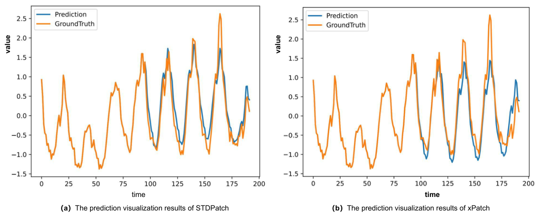
To intuitively demonstrate the prediction performance of the model under diverse data distributions, we conduct visual comparison experiments between the STDPatch and xPatch models on two benchmark datasets, namely Electricity and Traffic, with both the input and prediction lengths set to 96. On the Electricity dataset, which exhibits drastic fluctuations and prominent non-stationarity, the prediction curve of xPatch shows obvious amplitude attenuation and fitting lag at multiple peaks and troughs (e.g., around time steps 110, 140, and 160), as shown in Figure A1. This verifies the inherent limitation that the underlying EMA smoothing operator of xPatch tends to cause energy diffusion of local extreme values. In contrast, the prediction curve of STDPatch closely fits the violent oscillations of ground-truth values and accurately captures extreme peaks. The results indicate that the SG-Filter adopted by STDPatch effectively removes noise while preserving the extreme-value patterns of trend components. Meanwhile, its three-stream architecture enables precise decoupling and reconstruction of complex nonlinear mutations in time series.

Figure A1. Forecasting performance comparison of STDPatch and xPatch on the Electricity dataset.

Figure A1. Forecasting performance comparison of STDPatch and xPatch on the Electricity dataset.

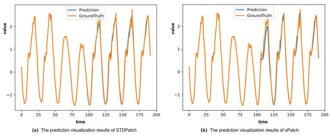
On the Traffic dataset with strong periodic patterns and relatively smooth trends, STDPatch also delivers outstanding fitting accuracy, as shown in Figure A2. Although xPatch can roughly capture the overall periodic trend, its prediction curve still suffers from slight amplitude deviation and morphological distortion at several local peaks, such as around time step 115. By comparison, the prediction curve of STDPatch closely matches the ground truth. This result demonstrates the effectiveness of the patch refactor module in alleviating morphological fragmentation caused by physical partitioning and restoring semantic consistency across patch boundaries. Combined with the visualization results on both datasets, STDPatch demonstrates superior prediction accuracy and robustness when handling both high-frequency fluctuating power load data and highly periodic traffic flow series.

Figure A2. Forecasting performance comparison of STDPatch and xPatch on the Traffic dataset.

Figure A2. Forecasting performance comparison of STDPatch and xPatch on the Traffic dataset.

References

- Luo, X.; Liu, D.; Kong, H.; Huai, S.; Chen, H.; Xiong, G.; Liu, W. Efficient deep learning infrastructures for embedded computing systems: A comprehensive survey and future envision. ACM Trans. Embed. Comput. Syst. 2024, 24, 21. [Google Scholar] [CrossRef] [Scilit]
- Zhou, H.; Zhang, S.; Peng, J.; Zhang, S.; Li, J.; Xiong, H.; Zhang, W. Informer: Beyond efficient transformer for long sequence time-series forecasting. In Proceedings of the AAAI Conference on Artificial Intelligence, Virtual, 2–9 February 2021; Volume 35, pp. 11106–11115. [Google Scholar] [CrossRef] [Scilit]
- Wang, H.; Zhang, X.; Xia, Y.; Wu, X. A differential privacy-preserving deep learning caching framework for heterogeneous communication network systems. Int. J. Intell. Syst. 2022, 37, 11142–11166. [Google Scholar] [CrossRef] [Scilit]
- He, H.; Zhang, Q.; Bai, S.; Yi, K.; Niu, Z. CATN: Cross attentive tree-aware network for multivariate time series forecasting. In Proceedings of the AAAI Conference on Artificial Intelligence, Virtual, 22 February–1 March 2022; Volume 36, pp. 4030–4038. [Google Scholar] [CrossRef] [Scilit]
- Chen, Z.; Ma, M.; Li, T.; Wang, H.; Li, C. Long sequence time series forecasting with deep learning: A survey. Inf. Fusion 2023, 97, 101819. [Google Scholar] [CrossRef] [Scilit]
- Wu, H.; Zhou, H.; Long, M.; Wang, J. Interpretable weather forecasting for worldwide stations with a unified deep model. Nat. Mach. Intell. 2023, 5, 602–611. [Google Scholar] [CrossRef] [Scilit]
- Jan, G.; Benidis, K.; Wang, Y.; Rangapuram, S.S.; Salinas, D.; Flunkert, V.; Bohlke-Schneider, M.; Januschowski, T. Probabilistic forecasting with spline quantile function RNNs. In Proceedings of the International Conference on Artificial Intelligence and Statistics (PMLR), Okinawa, Japan, 16–18 April 2019; pp. 1901–1910. [Google Scholar]
- Bai, S.; Kolter, J.Z.; Koltun, V. An empirical evaluation of generic convolutional and recurrent networks for sequence modeling. arXiv 2018, arXiv:1803.01271. [Google Scholar]
- Wu, H.; Hu, T.; Liu, Y.; Zhou, H.; Wang, J.; Long, M. TimesNet: Temporal 2D-variation modeling for general time series analysis. In Proceedings of the International Conference on Learning Representations, Kigali, Rwanda, 1–5 May 2023. [Google Scholar]
- Zeng, A.; Chen, M.; Zhang, L.; Xu, Q. Are transformers effective for time series forecasting? In Proceedings of the AAAI Conference on Artificial Intelligence, Kigali, Rwanda, 1–5 May 2023; Volume 37, pp. 11121–11128. [Google Scholar]
- Xu, Z.; Zeng, A.; Xu, Q. FITS: Modeling time series with 10k parameters. arXiv 2023, arXiv:2307.03756. [Google Scholar]
- Nie, Y.; Nguyen, N.H.; Sinthong, P.; Kalagnanam, J. A time series is worth 64 words: Long-term forecasting with transformers. In Proceedings of the International Conference on Learning Representations, Kigali, Rwanda, 1–5 May 2023. [Google Scholar]
- Liu, Y.; Hu, T.; Zhang, H.; Wu, H.; Wang, S.; Ma, L.; Long, M. iTransformer: Inverted transformers are effective for time series forecasting. In Proceedings of the International Conference on Learning Representations, Vienna, Austria, 7–11 May 2024. [Google Scholar]
- Wang, X.; Zhou, T.; Wen, Q.; Gao, J.; Ding, B.; Jin, R. CARD: Channel aligned robust blend transformer for time series forecasting. In Proceedings of the International Conference on Learning Representations, Vienna, Austria, 7–11 May 2024. [Google Scholar]
- Jin, M.; Wang, S.; Ma, L.; Chu, Z.; Zhang, J.Y.; Shi, X.; Chen, P.Y.; Liang, Y.; Li, Y.F.; Pan, S.; et al. Time-LLM: Time series forecasting by reprogramming large language models. In Proceedings of the International Conference on Learning Representations, Virtual, 3–7 May 2021. [Google Scholar]
- Zhou, T.; Niu, P.; Wang, X.; Sun, L.; Jin, R. One fits all: Power general time series analysis by pretrained LM. In Proceedings of the Advances in Neural Information Processing Systems, New Orleans, LA, USA, 10–16 December 2023; Volume 36, pp. 43322–43355. [Google Scholar]
- Wang, S.; Wu, H.; Shi, X.; Hu, T.; Luo, H.; Ma, L.; Zhang, J.Y.; Zhou, J. TimeMixer: Decomposable multiscale mixing for time series forecasting. arXiv 2024, arXiv:2405.14616. [Google Scholar]
- Stitsyuk, A.; Choi, J. xPatch: Dual-Stream Time Series Forecasting with Exponential Seasonal-Trend Decomposition. In Proceedings of the AAAI Conference on Artificial Intelligence, Philadelphia, PA, USA, 25 February–4 March 2025; Volume 39, pp. 20601–20609. [Google Scholar]
- Box, G.E.P.; Jenkins, G.M.; Reinsel, G.C.; Ljung, G.M. Time Series Analysis: Forecasting and Control; John Wiley & Sons: Hoboken, NJ, USA, 2015. [Google Scholar]
- Yu, G.; Zou, J.; Hu, X.; Aviles-Rivero, A.I.; Qin, J.; Wang, S. Revitalizing multivariate time series forecasting: Learnable decomposition with inter-series dependencies and intra-series variations modeling. arXiv 2024, arXiv:2402.12694. [Google Scholar]
- Wu, H.; Xu, J.; Wang, J.; Long, M. Autoformer: Decomposition transformers with auto-correlation for long-term series forecasting. In Advances in Neural Information Processing Systems; MIT Press: Cambridge, MA, USA, 2021; Volume 34, pp. 22419–22430. [Google Scholar]
- Zhou, T.; Ma, Z.; Wen, Q.; Wang, X.; Sun, L.; Jin, R. Fedformer: Frequency enhanced decomposed transformer for long-term series forecasting. In Proceedings of the International Conference on Machine Learning, Baltimore, MD, USA, 17–23 July 2022; pp. 27268–27286. [Google Scholar]
- Nematirad, R.; Pahwa, A.; Natarajan, B. Times2d: Multi-period decomposition and derivative mapping for general time series forecasting. In Proceedings of the AAAI Conference on Artificial Intelligence, Philadelphia, PA, USA, 25 February–4 March 2025; Volume 39, pp. 19651–19658. [Google Scholar]
- Chen, P.; Zhang, Y.; Cheng, Y.; Shu, Y.; Wang, Y.; Wen, Q.; Yang, B.; Guo, C. Pathformer: Multi-scale transformers with adaptive pathways for time series forecasting. arXiv 2024, arXiv:2402.05956. [Google Scholar]
- Savitzky, A.; Golay, M.J.E. Smoothing and differentiation of data by simplified least squares procedures. Anal. Chem. 1964, 36, 1627–1639. [Google Scholar] [CrossRef] [Scilit]
- Wang, R.; Miao, S.; Liu, D.; Jin, X.; Zhang, W. Multi-layer seasonal perception network for time series forecasting. In Proceedings of the ICASSP 2023—2023 IEEE International Conference on Acoustics, Speech and Signal Processing (ICASSP), Rhodes Island, Greece, 4–10 June 2023; pp. 1–5. [Google Scholar]
- Vizi, Z.; Batki, B.; Rátki, L.; Szalánczi, S.; Fehérváry, I.; Kozák, P.; Kiss, T. Water level prediction using long short-term memory neural network model for a lowland river: A case study on the Tisza River, Central Europe. Environ. Sci. Eur. 2023, 35, 92. [Google Scholar] [CrossRef] [Scilit]
- Wang, H.; Peng, J.; Huang, F.; Wang, J.; Chen, J.; Xiao, Y. MICN: Multi-scale local and global context modeling for long-term series forecasting. In Proceedings of the International Conference on Learning Representations, Kigali, Rwanda, 1–5 May 2023. [Google Scholar]
- Luo, D.; Wang, X. ModernTCN: A modern pure convolution structure for general time series analysis. In Proceedings of the International Conference on Learning Representations, Vienna, Austria, 7–11 May 2024. [Google Scholar]
- Oreshkin, B.N.; Carpov, D.; Chapados, N.; Bengio, Y. N-BEATS: Neural basis expansion analysis for interpretable time series forecasting. arXiv 2019, arXiv:1905.10437. [Google Scholar]
- Zhang, T.; Zhang, Y.; Cao, W.; Bian, J.; Yi, X.; Zheng, S.; Li, J. Less Is More: Fast Multivariate Time Series Forecasting with Light Sampling-oriented MLP Structures. arXiv 2022, arXiv:2207.01186. [Google Scholar]
- Challu, C.; Olivares, K.G.; Oreshkin, B.N.; Ramirez, F.G.; Canseco, M.M.; Dubrawski, A. N-HiTS: Neural hierarchical interpolation for time series forecasting. In Proceedings of the AAAI Conference on Artificial Intelligence, Washington, DC, USA, 7–14 February 2023; Volume 37, pp. 6989–6997. [Google Scholar]
- Huang, S.; Zhao, Z.; Li, C.; Bai, L. TimeKAN: KAN-based frequency decomposition learning architecture for long-term time series forecasting. arXiv 2025, arXiv:2502.06910. [Google Scholar]
- Woo, G.; Liu, C.; Sahoo, D.; Kumar, A.; Hoi, S. ETSformer: Exponential smoothing transformers for time-series forecasting. arXiv 2022, arXiv:2202.01381. [Google Scholar]
- Bao, Q.; Miao, S.; Tian, Y.; Jin, X.; Wang, P.; Jiang, Q.; Yao, S.; Hu, D.; Wang, R. GDRNet: A channel grouping based time-slice dilated residual network for long-term time-series forecasting. J. Supercomput. 2025, 81, 499. [Google Scholar]
- Lu, J.; Chen, P.; Guo, C.; Shu, Y.; Wang, M.; Yang, B. Towards Non-Stationary Time Series Forecasting with Temporal Stabilization and Frequency Differencing. In Proceedings of the AAAI Conference on Artificial Intelligence (AAAI), Singapore, 20–27 January 2026. [Google Scholar]
- Wang, Q.; Wu, Y.; Long, Y.; Huang, J.; Ran, F.; Su, B.; Xu, H. A Plug-and-Play Bregman ADMM Module for Inferring Event Branches in Temporal Point Processes. In Proceedings of the AAAI Conference on Artificial Intelligence (AAAI), Philadelphia, PA, USA, 25 February–4 March 2025. [Google Scholar]
- Wu, X.; Qiu, X.; Cheng, H.; Li, Z.; Hu, J.; Guo, C.; Yang, B. Enhancing time series forecasting through selective representation spaces: A patch perspective. arXiv 2025, arXiv:2510.14510. [Google Scholar]
- Zhang, W.; Yin, C.; Liu, H.; Zhou, X.; Xiong, H. Irregular Multivariate Time Series Forecasting: A Transformable Patching Graph Neural Networks Approach. In Proceedings of the International Conference on Machine Learning (ICML), Vienna, Austria, 21–27 July 2024. [Google Scholar]
- Liu, J.; Cao, M.; Chen, S. TimeCHEAT: A Channel Harmony Strategy for Irregularly Sampled Multivariate Time Series Analysis. In Proceedings of the AAAI Conference on Artificial Intelligence (AAAI), Philadelphia, PA, USA, 25 February–4 March 2025; pp. 18861–18869. [Google Scholar]
- Huang, Q.; Shen, L.; Zhang, R.; Cheng, J.; Ding, S.; Zhou, Z.; Wang, Y. HDMixer: Hierarchical Dependency with Extendable Patch for Multivariate Time Series Forecasting. In Proceedings of the AAAI Conference on Artificial Intelligence (AAAI), Vancouver, BC, Canada, 26–27 February 2024; pp. 12608–12616. [Google Scholar]
- Guo, T.; Xu, Z.; Yao, X.; Chen, H.; Aberer, K.; Funaya, K. Robust online time series prediction with recurrent neural networks. In Proceedings of the 2016 IEEE International Conference on Data Science and Advanced Analytics (DSAA), Montreal, QC, Canada, 17–19 October 2016; pp. 816–825. [Google Scholar]
- Pellicani, A.; Pio, G.; Džeroski, S.; Ceci, M. Dynamic instance weighting for online learning in multi-cryptocurrency price and trend forecasting. Data Min. Knowl. Discov. 2026, 40, 58. [Google Scholar] [CrossRef] [Scilit]
- Ashish, V.; Shazeer, N.; Parmar, N.; Uszkoreit, J.; Jones, L.; Gomez, A.N.; Kaiser, Ł.; Polosukhin, I. Attention is all you need. In Proceedings of the Advances in Neural Information Processing Systems, Long Beach, CA, USA, 4–9 December 2017; Volume 30. [Google Scholar]
- Paszke, A.; Gross, S.; Massa, F.; Lerer, A.; Bradbury, J.; Chanan, G.; Killeen, T.; Lin, Z.; Gimelshein, N.; Antiga, L.; et al. PyTorch: An Imperative Style, High-Performance Deep Learning Library. In Proceedings of the Advances in Neural Information Processing Systems, Vancouver, BC, Canada, 8–14 December 2019; Volume 32, pp. 8024–8035. [Google Scholar]
- Li, C.; Li, M.; Diao, R. TVNet: A Novel Time Series Analysis Method Based on Dynamic Convolution and 3D-Variation. arXiv 2025, arXiv:2503.07674. [Google Scholar]
Disclaimer/Publisher’s Note: The statements, opinions and data contained in all publications are solely those of the individual author(s) and contributor(s) and not of MDPI and/or the editor(s). MDPI and/or the editor(s) disclaim responsibility for any injury to people or property resulting from any ideas, methods, instructions or products referred to in the content. |
© 2026 by the authors. Licensee MDPI, Basel, Switzerland. This article is an open access article distributed under the terms and conditions of the Creative Commons Attribution (CC BY) license.