ExPAM: Explainable Personality Assessment Method Using Heterogeneous Linguistic Features and Off-the-Shelf LLMs

Abstract

Many organizations increasingly adopt personalization techniques to enhance user satisfaction. However, current systems generally cannot automatically infer and interpret individual personality traits (PTs), although these traits are key drivers of user behavior. While Large Language Models (LLMs) are widely used, they remain poorly suited to reliable and explainable Personality Assessment (PA). To address this gap, we propose ExPAM, a novel Explainable Personality Assessment Method that combines hybrid feature fusion with in-context learning in off-the-shelf LLMs to predict Big Five PTs from text. ExPAM explicitly grounds its predictions in interpretable linguistic patterns without requiring LLM fine-tuning. Its hybrid fusion is designed to improve both predictive performance and interpretability in PA. Transformer-based embeddings encode local contextual information, whereas features extracted using the Linguistic Inquiry and Word Count (LIWC) dictionary provide complementary global and local linguistic indicators of PTs. These interpretable feature patterns are included in prompts that guide the LLM to produce both PT predictions and human-understandable explanations. ExPAM shows competitive performance compared with multi-task models on the ChaLearn First Impressions v2 (FIv2) corpus and single-task models on the PANDORA corpus that rely on a single feature set. On FIv2, it achieves a mean accuracy (mAC) of 0.891 and a Concordance Correlation Coefficient (CCC) of 0.333. On PANDORA, it achieves a mean Pearson Correlation Coefficient (PCC) of 0.240 and a CCC of 0.101. Prompting the LLM with hybrid global–local patterns further improves CCC by 9.9% on FIv2 and 15.8% on PANDORA, while changes in mAC and mean PCC remain marginal. Qualitative interpretability analysis reveals trait-specific linguistic patterns, highlighting the potential of ExPAM for psychological research, computational linguistics, and paralinguistic studies.

1. Introduction

Personality Traits (PTs) are stable patterns of thought, feeling, and behavior that distinguish individuals. The Big Five personality model, also known as OCEAN, is widely used in computer science and psychology [1]. It includes five personality traits (PTs): Openness to experience (O), Conscientiousness (C), Extroversion (E), Agreeableness (A), and Neuroticism/non-Neuroticism (N), which influence various aspects of behavior [2]. Personality Assessment (PA) plays a key role in understanding human behavior and is used in a wide range of domains, including health monitoring [3], education [4], marketing [5], and human resources [6,7,8].

Researchers use various modalities, such as audio, video, and text, to analyze PTs, as well as bimodal and multimodal fusion strategies that combine two or more sources of information [9,10]. The present work focuses exclusively on the text modality, since the availability and abundance of textual data from digital platforms, such as social media, personal messages, and professional documents, make it informative for real-world applications [11,12]. Importantly, text is characterized by its verbal nature, as it directly reflects an individual’s cognitive or linguistic style, allowing traits to be analyzed through lexical and semantic content [13].

Traditional text-based PA methods rely on hand-crafted lexical features, such as word counts, sentiment, or word category associations. Such features are often extracted from well-known psycholinguistic tools such as Linguistic Inquiry and Word Count (LIWC) [14]. Methods based on hand-crafted features can explain which words are associated with PTs, offering interpretable models to understand relationships between linguistic patterns and PTs [15]. However, such methods are often less reliable than methods based on deep features, which capture contextual and semantic nuances [16]. Methods based on deep features, especially those using pre-trained language models such as Bidirectional Encoder Representations from Transformer (BERT)-based and Word2Vec, produce rich contextual embeddings that encode syntactic, semantic, and pragmatic information. They effectively capture complex linguistic patterns in PT [17,18,19].

To combine both deep and hand-crafted features, temporal models such as Recurrent Neural Networks (RNNs), Long Short-Term Memory (LSTM), and Transformer are commonly used [13,18]. These models capture sequential dependencies in textual data and analyze how linguistic patterns unfold over time. Despite recent progress in PA, current methods often rely on a single feature set, which limits the interpretability of the model. To address this limitation, interpretation methods such as SHapley Additive exPlanations, Local Interpretable Model-agnostic Explanations, and Large Language Models (LLMs) are used [20,21,22,23]. However, the first two methods do not support all model architectures, while off-the-shelf LLMs often require fine-tuning. In-context learning [24,25] offers a flexible alternative to fine-tuning for personality inference [26,27], although performance remains sensitive to phrasing and prompt design.

This paper addresses these research gaps and aims to improve the performance and interpretability of PA by developing ExPAM, an Explainable Personality Assessment Method based on hybrid linguistic feature modeling. To make the methodological structure clearer, we distinguish the core contribution of ExPAM from auxiliary components used for implementation, comparison, and evaluation. The core mechanism of ExPAM consists of three components: deep feature analysis, hand-crafted feature analysis, and interpretation. The first two components model complementary linguistic information using deep contextual representations and interpretable psycholinguistic categories, respectively. To capture linguistic patterns over time, these components use Bidirectional LSTM (BiLSTM)-based and Mamba-based [28] models with an attention mechanism. The interpretation component computes gradient-based importance scores for words, tokens, and word categories, and the resulting explainable outputs are then used as prompts for an off-the-shelf LLM. Thus, the main novelty of ExPAM lies in a unified pipeline that connects hybrid linguistic representation learning, multi-task OCEAN prediction, gradient-based explanation generation, and LLM-based refinement without fine-tuning off-the-shelf LLMs for PA. In contrast, components such as BERT [29], XLM-RoBERTa [30], jina-embeddings-v3 [31] (JINA), LIWC [14], BiLSTM, and Mamba [28] are used as feature extractors, linguistic resources, or model variants within the proposed method. This design directly follows from three gaps identified in State-of-the-Art (SOTA) work: the limited use of complementary deep and hand-crafted linguistic features in a unified model, the lack of transparent token-level and category-level explanations for text-based PA, and the insufficient understanding of whether model-derived explanations can serve as structured prompts for off-the-shelf LLMs. Specifically, we address the following research questions:

• RQ1: Can hybrid fusion that combines hand-crafted and deep linguistic features improve both prediction performance and interpretability in PA?
• RQ2: Can gradient-based interpretation be adapted to textual data to explain PT predictions through token-level and LIWC-category-level evidence?
• RQ3: Can explanations generated by the proposed model effectively serve as in-context prompts for LLMs to improve PTs prediction performance without fine-tuning?

Our main contributions are as follows:

• An Explainable Personality Assessment Method (ExPAM) through hybrid fusion of linguistic features.
• Explainable outputs produced by ExPAM are used as prompts to guide LLM-based predictions.
• A comparative analysis of twelve off-the-shelf LLMs across various in-context learning setups, including zero-shot, one-shot, and few-shot, as well as explanation-based setups.

2. Related Work

2.1. State-of-the-Art Methods

SOTA text-based methods for PA are largely limited to a single feature set, either hand-crafted or deep ones, and do not provide explainability without fine-tuning an off-the-shelf LLM for a specific task. In 2017, a challenge was organized to develop PA methods using video interviews [32]; for this purpose, a new corpus called ChaLearn First Impressions v2 (FIv2) was introduced. Later, the same authors [33] used the NLTK toolkit to extract eight readability measures and supplemented them with total word count and the number of unique words in transcripts. Logistic Regression (LR) was applied to predict the five PTs for each feature set. In contrast, Aslan et al. [34] used pre-trained Embeddings from Language Models (ELMo) with Fully Connected Layers (FCLs) and achieved similar results. Suman et al. [35] compared several word representation models, such as Global Vectors (GloVe), BERT, Text-char-1, and Text-char-2, whose embeddings were fed into a Convolutional Neural Network (CNN) and FCL to predict five PT scores, achieving performance comparable to previous methods. Ouarka et al. [36] and Revathi et al. [37] also used GloVe with a combination of CNNs and FCLs, while Wang et al. [18] extracted linguistic features using Contrastive Language-Image Pretraining (CLIP)-based [38] visual–text associations. Finally, Bounab et al. [13] fine-tuned neural feature extractors, including Word2Vec, Doc2Vec, and Facebook’s FastText, and used five separate BiLSTM-based temporal models with self-attentions. Each model contains a single-task regressor, which excludes correlations between traits. In addition, they first trained the entire pipeline on job interview estimation before adapting it to PA.

For PA on the PANDORA corpus, Gjurković et al. [39] used n-grams, Myers–Briggs Type Indicator (MBTI) dimensions, and psycholinguistic features with an LR model, while still predicting each PT separately. Radisavljević et al. [40] extended this approach with Enneagram predictions and specific LIWC features, and compared several regressors, including Ridge, Elastic-Net, Huber, and Support Vector Regression. Fu et al. [41] fine-tuned the Language Understanding with Knowledge-based Embeddings (LUKE) transformer-based model with a regression head as an auxiliary personality predictor for empathetic response generation. More recent studies shifted toward transformer-based continuous prediction. Killian Jr and Sun [42] fine-tuned a BERT-based regressor with a shared [CLS] representation for all five PTs. Wang and Sun [43] used RoBERTa with mixed training strategies and a Multilayer Perceptron (MLP) head. Maharjan et al. [22] compared BERT, RoBERTa, and OpenAI’s text-embedding-3-small within a BiLSTM-based model and additionally evaluated their psychometric validity through correlations with LIWC and emotion-related features. Shum et al. [44] fine-tuned BERT and RoBERTa and analyzed intercorrelations among PTs. Shen et al. [45] proposed the self-supervised EmoPerso framework with synthetic augmentation, auxiliary affective features, and cross-attention. Finally, Aragón et al. [46] compared Bag-of-Words (BoW), DisorBERT, and MPNet representations and trained five separate models for each PT, showing that a simple BoW+Support Vector Machine (SVM) model achieved the highest Pearson Correlation Coefficient (PCC) across all five PTs.

Despite a high recognition accuracy, the methods [13,39,40,41,46] are based on separate models for each trait, which limits their ability to explicitly model dependencies between PTs. In addition, most of these approaches offer limited interpretability, which limits their applicability in practical settings.

2.2. Interpretation Methods

Interpretable methods are crucial for PA, given the sensitive and complex nature of PT inferences [11,47]. Traditional interpretability methods, such as Local Interpretable Model-agnostic Explanations [48] and SHapley Additive exPlanations [49], are widely used in machine learning [50,51]. However, these methods have notable limitations for PA. The PA models often involve high-dimensional linguistic features and multi-task learning. Zhao et al. [52] noted that standard attention visualization tools do not provide a theoretical explanation for predictions, underscoring the need for more interpretable methods. LLMs can generate more natural and context-aware explanations for PT inferences. The idea is that an LLM, with its strong language abilities and capacity for human-like communication, can articulate the reasoning behind a PA model’s outputs in a human-readable form. Sun et al. [20] introduced a “chain-of-personality-evidence” method, in which a GPT-4-based system identifies dialogue excerpts indicative of an individual’s traits and then composes a summary explanation connecting this evidence to the Big Five prediction. Wen et al. [21] proposed Affective Natural Language Inference (Affective-NLI), which enriches text with personality descriptions, allowing pre-trained LMs to provide explainable results. Although a gap remains between current explanations and human-level explanations, integrating LLMs into PA helps narrow this gap.

3. Materials

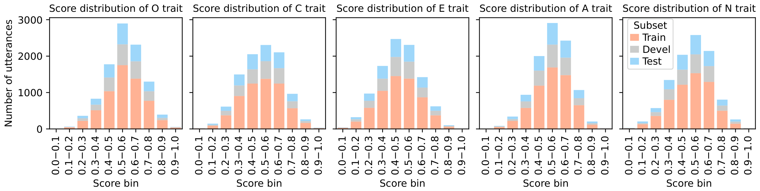
In this work, we conduct experiments on two corpora: the large-scale multimodal FIv2 (ChaLearn First Impressions v2) corpus (https://chalearnlap.cvc.uab.cat/dataset/24/description/, accessed on 13 July 2026) [33] and the text-only PANDORA (Personality ANd Demographics Of Reddit Authors) corpus (https://psy.takelab.fer.hr/datasets/all/PANDORA/, accessed on 13 July 2026) [39]. FIv2 comprises 10K short high-definition video clips from YouTube with about 3K unique individuals. Each video is in English and lasts about 15 s. Each video is annotated with scores for each PT ranging from 0 to 1. The corpus is divided into three main subsets: Train (6K videos), Development (2K videos), and Test (2K videos). Figure 1 shows the score distributions for the O, C, E, A, and N traits in the Train, Development, and Test subsets. The scores for four of the five PTs (O, C, A, and N) are concentrated between 0.4 and 0.6, while the scores for E are concentrated between 0.3 and 0.5. This central tendency may cause the model to predominantly predict mean values, which may reduce performance for instances with low or high PT scores [33]. The corpus ensures diversity by including people of varying genders, ages, and ethnicities. This broad demographic representation, combined with a variety of monologue topics, improves the real-world applicability of models trained on FIv2.

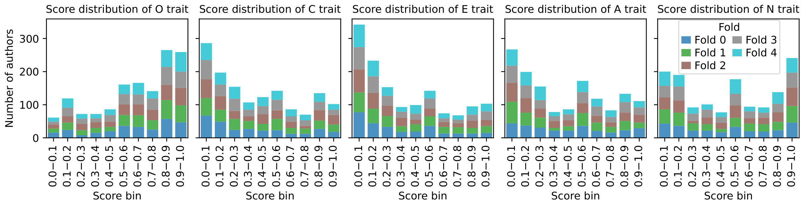
PANDORA contains approximately 2.8M English Reddit comments from about 1.4K authors with PT annotations [39]. In contrast to FIv2, we use predefined author-level folds from the official baseline split. Therefore, instead of fixed Train/Development/Test subsets, we perform a fold-based training and evaluation. For comparability with FIv2, PANDORA trait scores are mapped from $[0,100]$ to $[0,1]$, and Neuroticism is converted to non-Neuroticism as $1-N$. Moreover, unlike SOTA methods developed on this corpus, we train both single-task and multi-task models. Figure 2 shows the distribution of PT scores across authors in the predefined folds. In contrast to FIv2, where most scores are concentrated in the range $[0.4,0.6]$, the PANDORA score distributions are generally more balanced across bins, with a slight shift toward higher values $[0.8,1]$ for O and toward lower values $[0,0.2]$ for C, E, and A.

Other text-only corpora include the Essays corpus [53] (2500 student essays with self-reported PTs), myPersonality [54] (66K Facebook users linked to 22M status updates and questionnaire scores), and dialogue-based corpora, such as Story2Personality [55] (3543 characters extracted from 507 movie scripts with dialogue and scene descriptions) and PersonalityEvd [20] (about 2K dialogues from 72 users). These corpora remain valuable benchmarks. Among text-only corpora, PANDORA stands out for its scale and labeling setup, providing a large number of comments per user, enabling more stable user-level (or author-level) modeling than smaller alternatives. Its domain, naturalistic Reddit discourse, complements and extends that of FIv2, which consists of short video interviews. This allows us to evaluate the proposed method across multiple domains and to assess the cross-corpus robustness of models trained on different corpora.

For FIv2, the preprocessing stage begins with speech transcriptions produced by an Automatic Speech Recognition (ASR) system, specifically the Whisper model [56]. Following transcription, we apply a standard text normalization pipeline. The pipeline converts all input text to lowercase, expands frequent English contractions (e.g., don’t → do not), removes punctuation, and deletes annotations enclosed in square brackets (e.g., non-linguistic markers or editorial notes). In general, these steps reduce spelling variability and remove extraneous characters, resulting in clean and uniformly formatted text for subsequent analysis.

4. Methods

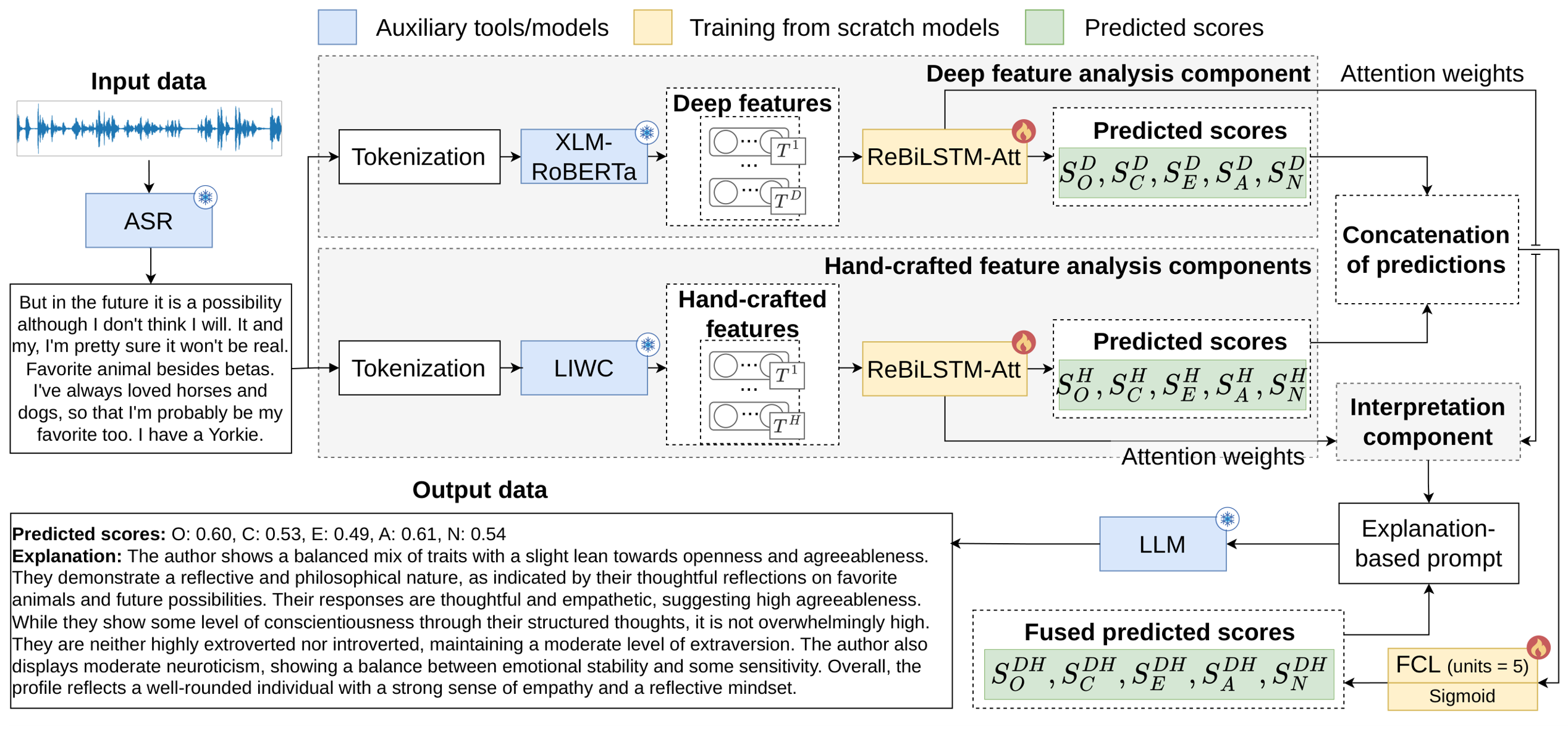
Figure 3 shows the ExPAM pipeline. The input is a textual speech transcription obtained after ASR using Whisper [56]. The deep and hand-crafted feature analysis components produce five predicted PT scores and attention outputs. Their predictions are concatenated and passed to the final FCL with five units to obtain the fused scores. The interpretation component then identifies important words, tokens, and word categories, supporting qualitative analysis and the optional LLM-based calibration stage. The contribution of each component and of their fusion is evaluated through ablation studies. All components of ExPAM are described below.

Overall, the methodological contribution of ExPAM lies in its core mechanism, which jointly performs hybrid linguistic modeling, multi-task PT prediction, prediction-level fusion, and gradient-based explanation generation. In contrast, Whisper, XLM-RoBERTa, the LIWC dictionary, and off-the-shelf LLM are used as supporting components for transcription, deep and hand-crafted feature extraction, and optional score calibration, respectively.

4.1. Deep and Hand-Crafted Feature Analysis Components

In the first step of both components, an input text is tokenized. In the deep feature analysis component, a multilingual XLM-RoBERTa model [30] is used to extract deep word representations (or deep features). Unknown or long words are split into sub-tokens using the WordPiece tokenization algorithm used by XLM-RoBERTa. A unique identifier is assigned to each (sub-)token. The vector of unique identifiers is passed through the XLM-RoBERTa model to extract a feature matrix with a size of $T\times 768$, where T is the number of (sub-)tokens including two special tokens. The value of T varies across utterances; therefore, during training, we pad sequences with zeros to the maximum length within a batch and apply a mask to ignore the padded (sub-)tokens.

In the hand-crafted feature analysis component, the LIWC [14] dictionary is used to extract features from English words. LIWC is designed for psychological text analysis. In this dictionary, words are grouped into 64 categories, such as work, cognitive processes, and anxiety, among others. Each word can belong to more than one category and is represented as a binary feature vector. Each value in the feature vector is encoded with 1 if a word belongs to the corresponding LIWC category and with 0 otherwise. These feature vectors are formed as a feature matrix with a size of $T\times 64$. For this feature set, a length-based mask is also applied in the same manner as for the previous one.

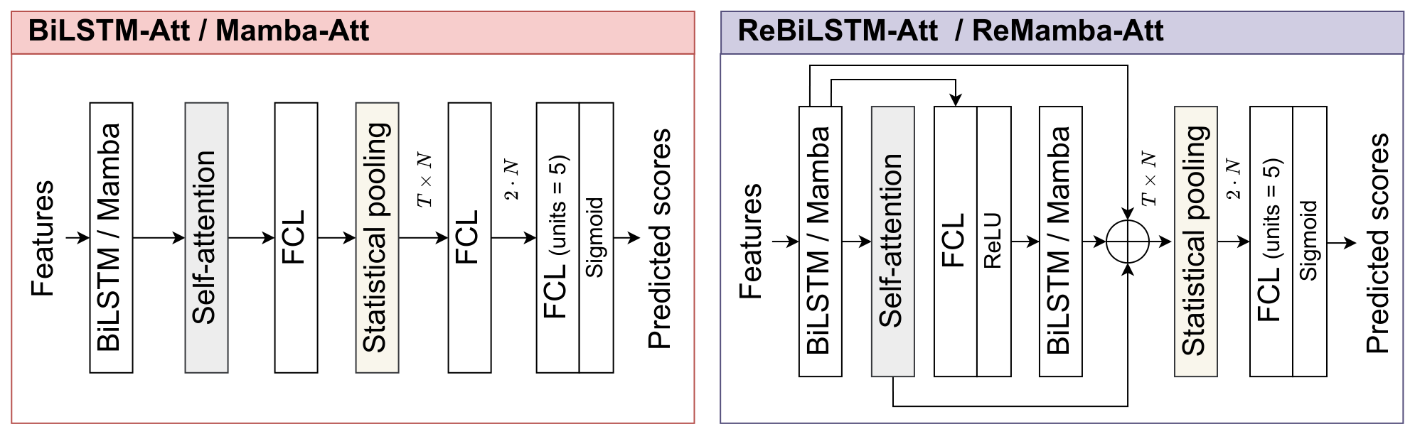
We consider four models for contextual modeling of individual PTs. The proposed linguistic models are shown in Figure 4. All architectures include temporal layers, a self-attention [57] mechanism, and a statistical pooling layer. We use BiLSTM and Mamba [28] to learn context from the feature representations. The former captures sequential dependencies via gated recurrent mechanisms with bidirectional context integration and can adapt the dimension of its hidden states to the desired output size. The latter, in contrast, relies on a selective state-space mechanism with linear-time inference while keeping a fixed hidden size; therefore, a linear projection layer is added after the Mamba block to map its output to the target dimension. Both models efficiently process long sequences. The self-attention mechanism helps the model focus on informative parts of the input sequence. Statistical pooling aggregates sequential data while preserving the mean and standard deviation of feature variations. In addition, ReBiLSTM-Att and ReMamba-Att use a residual connection that improves gradient flow during training.

The deep feature analysis component is based on the pre-trained XLM-RoBERTa model and produces rich feature representations trained on large-scale data. In contrast, the hand-crafted feature analysis component relies on predefined linguistic rules and domain-specific knowledge embedded in LIWC, which organizes text into structured categories based on linguistic and psychological attributes. Thus, deep features study non-linear relationships between words, while hand-crafted features study psycholinguistic patterns.

4.2. Interpretation Component

We use the attention outputs of the proposed models together with gradient-based importance scores to analyze the contribution of words, tokens, and word categories to the prediction of the five PTs. Since LIWC groups words into 64 categories, the hand-crafted feature analysis component enables both local analysis within an utterance and global analysis across utterances. In contrast, the deep feature analysis component supports token-level analysis. Unlike frequency-based explanations used in previous works [13,20], our results suggest that model-derived importance scores may better reflect the evidence used by the prediction model than raw word frequency alone.

The importance of words, tokens, and word categories is computed by adapting Grad-CAM [58] to the BiLSTM- and Mamba-based models. The resulting heatmaps are treated as local sensitivity maps derived from the trained ExPAM model. They should not be interpreted as causal explanations of the full decision-making mechanism. Rather, they indicate how changes in input features may affect the predicted score of a particular PT. Thus, the generated explanations are used as model-derived evidence for interpretation and LLM prompting, but not as independent psychological justifications.

Formally, ExPAM solves the mapping $f:\mathbb{X}\to \mathbb{S}$, where $\mathbb{X}$ is the input utterance and $\mathbb{S}\subseteq {\mathbb{R}}^5$ is the vector of predicted scores for the five PTs. We denote the model output by $\mathit{S}=[S_O,S_C,S_E,S_A,S_N]\in {\mathbb{R}}^5$. The input utterance is represented by two feature matrices: the deep feature matrix ${\mathit{F}}^D={[{\mathit{f}}_1^D,\dots ,{\mathit{f}}_{T^D}^D]}^{\top }\in {\mathbb{R}}^{T^D\times N^D}$ and the hand-crafted feature matrix ${\mathit{F}}^H={[{\mathit{f}}_1^H,\dots ,{\mathit{f}}_{T^H}^H]}^{\top }\in {\mathbb{R}}^{T^H\times N^H}$, where $T^D$ and $T^H$ are the numbers of (sub-)tokens and tokens, respectively, and $N^D$ and $N^H$ are the corresponding feature dimensions.

For the deep feature analysis component, the model receives ${\mathit{F}}^D$ and produces ${\mathit{S}}^D\in {\mathbb{R}}^5$. For each trait $k\in \{1,\dots ,5\}$, the deep-feature gradient map is defined as

$${\mathit{FM}}_k^D={\displaystyle \frac{\partial S_k^D}{\partial {\mathit{F}}^D}}\in {\mathbb{R}}^{T^D\times N^D}.$$

(1)

This map is aggregated into the token-level importance vector ${\widetilde{\mathit{FM}}}_k^D\in {\mathbb{R}}^{T^D}$ and is then merged at the word level when sub-tokens belong to the same word. The detailed aggregation procedure is given in Appendix A.

For the hand-crafted feature analysis component, the model receives ${\mathit{F}}^H$ and produces ${\mathit{S}}^H\in {\mathbb{R}}^5$. The category-level gradient map for trait k is computed as

$${\mathit{FM}}_k^H={\displaystyle \frac{\partial S_k^H}{\partial {\mathit{F}}^H}}\in {\mathbb{R}}^{T^H\times N^H}.$$

(2)

After averaging over token positions, categories absent from the utterance are masked. The resulting local hand-crafted importance vector is denoted by ${\widetilde{\mathit{FM}}}_k^H\in {\mathbb{R}}^{N^H}$. Global category-level importance is then obtained by averaging these local masked vectors over the Train subset:

$${\widetilde{\mathit{GFM}}}_k^H={\displaystyle \frac{1}{M}}{\displaystyle \sum _{m=1}^M}{\widetilde{\mathit{FM}}}_k^{H\left(m\right)}\in {\mathbb{R}}^{N^H},$$

(3)

where M is the number of utterances in the Train subset and ${\widetilde{\mathit{FM}}}_k^{H\left(m\right)}$ is the masked importance vector for trait k computed on the m-th utterance. In this way, ExPAM provides local token-level and category-level explanations, as well as global LIWC-category-level summaries for each PT.

4.3. LLM Integration

The interpretation produced by our hybrid feature-based model still requires clarification and humanization of the results. To address this issue, we employ off-the-shelf LLMs. We evaluate LLMs independently of our method in three different in-context learning experimental setups:

1.

Zero-shot, in which the model predicts scores for five PTs using only a single test utterance;

2.

One-shot, in which the model receives one test and one annotated utterance;

3.

Few-shot, in which the model makes predictions based on five annotated utterances.

In the final setup, called the explanation-based setup, we evaluate the most efficient LLM in combination with our hybrid feature-based method, using the generated explainable output of the method as a prompt for the LLM. The LLM makes predictions only for the Test subset, while annotated utterances from the Train subset are used as examples. We also use the default settings for all used off-the-shelf LLMs considered in this work.

It should be emphasized that the explanation-based setup is not intended to make the LLM predict personality from scratch. Instead, it is formulated as a constrained score calibration procedure. The preliminary ExPAM scores are used as anchors, while the generated trait-specific explanations determine the magnitude of score correction. The transcript is used only as an additional weak constraint and cannot override the correction direction defined by the preliminary score. Therefore, the observed improvement in this setup should be interpreted as the effect of explanation-guided calibration rather than as the result of unconstrained LLM reasoning.

4.4. Evaluation Method

To evaluate the models, we use different performance measures depending on the corpus. For FIv2, the official evaluation measures are Accuracy (AC) [33] and mean accuracy (mAC), whereas for PANDORA, the official evaluation measures are PCC [39] and mean PCC (mPCC). In addition, we report Concordance Correlation Coefficient (CCC) [59] as a supplementary measure to provide a more comprehensive assessment of the agreement between predicted and ground truth scores. AC measures the error between predicted and ground truth scores, whereas PCC and CCC assess their linear association and concordance, respectively. mAC is the average of all AC measures for each PT $i\in \{1,\dots ,5\}$ [60]:

$$A{c}^{\left(i\right)}=1-{\displaystyle \frac{1}{U}}{\displaystyle \sum _{u=1}^U}\left|y_u^{\left(i\right)}-{\widehat{y}}_u^{\left(i\right)}\right|,$$

(4)

$$mAc={\displaystyle \frac{1}{5}}{\displaystyle \sum _{i=1}^5}A{c}^{\left(i\right)},$$

(5)

where U is the number of test utterances; $y_u^{\left(i\right)}$ and ${\widehat{y}}_u^{\left(i\right)}$ denote the ground truth and the predicted scores, respectively, for the PT i of the test utterance u.

For PANDORA, PCC for each PT is computed as follows:

$${\rho }^{\left(i\right)}={\displaystyle \frac{\mathrm{cov}\left(y^{\left(i\right)},{\widehat{y}}^{\left(i\right)}\right)}{{\sigma }_{y^{\left(i\right)}}{\sigma }_{{\widehat{y}}^{\left(i\right)}}}},$$

(6)

$$mPCC={\displaystyle \frac{1}{5}}{\displaystyle \sum _{i=1}^5}{\rho }^{\left(i\right)},$$

(7)

where ${\rho }^{\left(i\right)}$ is the PCC for the PT i, and $mPCC$ is the average PCC across all five PTs.

The CCC is computed as follows:

$$CCC={\displaystyle \frac{2{\rho }_{y,\widehat{y}}{\sigma }_y{\sigma }_{\widehat{y}}}{{\sigma }_y^2+{\sigma }_{\widehat{y}}^2+{\left({\mu }_y-{\mu }_{\widehat{y}}\right)}^2}},$$

(8)

where y and $\widehat{y}$ are the ground truth and the predicted scores over all test utterances U of all PTs; ${\mu }_y$ and ${\mu }_{\widehat{y}}$ denote the means of the ground truth and the predicted scores; ${\sigma }_y$ and ${\sigma }_{\widehat{y}}$ are the corresponding standard deviations; and ${\rho }_{y,\widehat{y}}$ is the PCC between y and $\widehat{y}$.

For FIv2, we used the official author-independent split into the Train, Development, and Test subsets. The models were trained on the Train subset, their hyperparameters were selected on the Development subset, and the best configuration was finally evaluated on the Test subset.

For PANDORA, we followed the official five-fold cross-validation protocol. In each run, one fold was used for testing, one for validation, and the remaining three for training. This procedure was repeated until each fold had served as the test fold once. For this corpus, we report both the mean and standard deviation of the performance measures across the five folds.

The performance comparison of the proposed method and comparison with SOTA methods is presented in Section 5.2.

5. Experiments

5.1. Experimental Setup

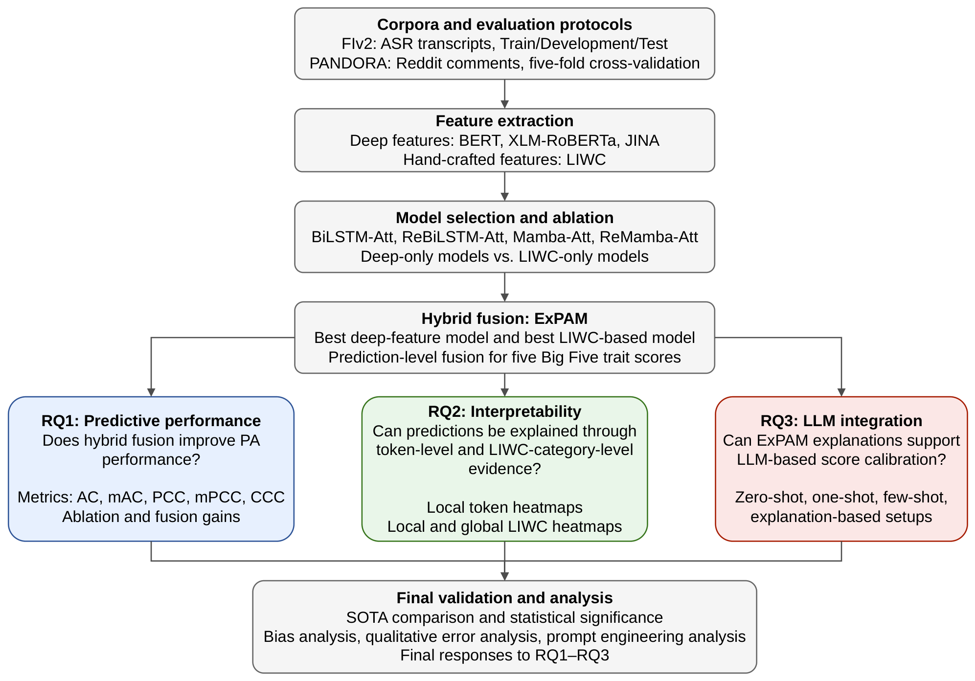
Figure 5 summarizes the experimental setup. We first compare deep word representations and temporal architectures, then evaluate LIWC-based models, fuse the best deep-feature and hand-crafted feature configurations into ExPAM, analyze local and global heatmaps, and finally test zero-shot, one-shot, few-shot, and explanation-based LLM prompting setups. These stages correspond to RQ1–RQ3 and are followed by SOTA comparison, statistical testing, bias analysis, and qualitative error analysis.

During the model training, the optimal model and training parameters are selected using the grid search method. The following parameters are considered: (1) the number of units in LSTM {32, 64, 128, 256}; (2) the number of units in FCL {64, 128, 256, 512}; (3) the optimizer {Adam, SGD, AdamW}; and (4) the learning rate $\{{10}^{-3},{10}^{-4},{10}^{-5}\}$. For reproducibility, the random seed was set to 42. To support replicability, the source code of ExPAM is publicly available at https://github.com/SMIL-SPCRAS/ExPAM (accessed on 13 July 2026) and includes the main pipeline implementation, configuration files, and the list of required libraries. We set the batch size to 32 and train for up to 500 epochs, using early stopping with a patience of 100 epochs based on validation performance. The proposed models were trained on an NVIDIA GeForce RTX 3090, while LLMs were run on an NVIDIA A100. The use of a fixed random seed and the detailed reporting of the experimental configuration support the reproducibility. Nevertheless, minor numerical variations may still occur across different hardware and software environments due to the non-deterministic nature of some GPU operations.

5.2. Experimental Results

Table 1. Performance comparison of the proposed methods on the FIv2 corpus. ZS, OS, FS and EX mean zero-shot, one-shot, few-shot, and explanation-based setups, respectively. CCC reports the absolute performance value, while ${\Delta }_{\mathrm{CCC}}$ reports the relative percentage change in CCC compared with the baseline method, JINA + BiLSTM-Att. The best results are highlighted in bold.

ID	Method	AC					mAC, %	CCC	${\mathbf{\Delta }}_{\mathbf{CCC}}$, %
		O	C	E	A	N
1	JINA + BiLSTM-Att	0.889	0.887	0.883	0.897	0.884	0.888	0.286	–
2	JINA + ReBiLSTM-Att	0.889	0.886	0.885	0.897	0.884	0.888	0.238	$-16.8$
3	JINA + Mamba-Att	0.890	0.888	0.885	0.898	0.884	0.889	0.255	$-10.8$
4	JINA + ReMamba-Att	0.891	0.887	0.885	0.897	0.884	0.889	0.276	$-3.5$
5	XLM-RoBERTa + BiLSTM-Att	0.891	0.889	0.886	0.899	0.887	0.890	0.304	6.3
6	XLM-RoBERTa + ReBiLSTM-Att	0.892	0.889	0.887	0.900	0.888	0.891	0.311	8.7
7	XLM-RoBERTa + Mamba-Att	0.891	0.889	0.886	0.900	0.887	0.890	0.300	4.9
8	XLM-RoBERTa + ReMamba-Att	0.891	0.889	0.886	0.900	0.886	0.890	0.316	10.5
9	BERT + BiLSTM-Att	0.890	0.887	0.885	0.899	0.885	0.889	0.293	2.4
10	BERT + ReBiLSTM-Att	0.891	0.887	0.885	0.899	0.885	0.889	0.294	2.8
11	BERT + Mamba-Att	0.890	0.887	0.884	0.899	0.884	0.889	0.276	$-3.5$
12	BERT + ReMamba-Att	0.890	0.887	0.885	0.899	0.886	0.889	0.297	3.8
13	LIWC + BiLSTM-Att	0.890	0.884	0.884	0.899	0.886	0.889	0.263	$-8.0$
14	LIWC + ReBiLSTM-Att	0.889	0.885	0.885	0.900	0.886	0.889	0.289	1.0
15	LIWC + Mamba-Att	0.889	0.883	0.884	0.898	0.884	0.888	0.245	$-14.3$
16	LIWC + ReMamba-Att	0.889	0.884	0.883	0.898	0.885	0.888	0.261	$-8.7$
17	IDs 6 and 14	0.892	0.889	0.887	0.901	0.888	0.891	0.333	16.4
18	Gemma4-31B ZS	0.879	0.874	0.852	0.862	0.828	0.859	0.138	$-51.7$
19	Gemma4-31B OS	0.875	0.872	0.852	0.863	0.832	0.859	0.155	$-45.8$
20	Gemma4-31B FS	0.867	0.872	0.863	0.858	0.838	0.860	0.167	$-41.6$
21	ID 17 + Gemma4-31B EX	0.891	0.888	0.886	0.900	0.887	0.890	0.366	$28.0$

presents the experimental results on FIv2 for the proposed methods based on different combinations of features (BERT [29], XLM-RoBERTa [30], JINA [31]) and model variants. It also reports the results obtained with LLMs. The mAC measure does not show significant performance differences compared with CCC. Therefore, further performance comparisons are based on the CCC measure, while mAC is used for comparison with the SOTA methods.

Among deep feature representations, XLM-RoBERTa achieved the highest performance across the trained model variants. Its larger number of parameters (278M) relative to BERT (178M) and JINA (129M) may contribute to richer contextual representations in this setting. JINA (30 languages) underperformed XLM-RoBERTa (100 languages) and BERT (104 languages), which may be related to differences in multilingual exposure and pre-training objectives. At the same time, the fact that BERT has broader language coverage but lower performance than XLM-RoBERTa suggests that parameterization and representation quality may be at least as important as the number of supported languages for text-based PA. The best mAC was achieved using XLM-RoBERTa + ReBiLSTM-Att ($\mathrm{mAC}=0.891$; ${\Delta }_{\mathrm{mAC}}=0.3\%$ relative to JINA + BiLSTM-Att), while the best CCC was obtained with XLM-RoBERTa + ReMamba-Att ($\mathrm{CCC}=0.316$; ${\Delta }_{\mathrm{CCC}}=10.5\%$). Models based on hand-crafted features were generally weaker than the best XLM-RoBERTa- and BERT-based configurations. Among them, LIWC + ReBiLSTM-Att achieved $\mathrm{mAC}=0.889$ (${\Delta }_{\mathrm{mAC}}=0.1\%$) and $\mathrm{CCC}=0.289$ (${\Delta }_{\mathrm{CCC}}=1.0\%$). Mamba-based models showed lower performance with binary LIWC features, while with deep features their results were comparable to those of BiLSTM-based variants.

In general, models with residual connections and two temporal layers (ReBiLSTM-Att and ReMamba-Att) tended to outperform their non-residual versions (BiLSTM-Att and Mamba-Att). This may indicate that additional depth and residual connections contribute to performance, although the effect also depends on the temporal layer. BiLSTM yielded higher and more stable gains than Mamba in these text-based PA experiments. This may suggest that bidirectionality and recurrence capture long-range context more effectively than selective state-space mechanisms. Therefore, we combine the predictions of XLM-RoBERTa + ReBiLSTM-Att and LIWC + ReBiLSTM-Att in the final fusion. Combining these two methods (IDs 6 and 14) at the prediction level yielded a 7.1% relative improvement in CCC (CCC of 0.311 vs. 0.333). Thus, the fusion of deep and hand-crafted features mainly improves CCC, while the change in mAC remains marginal.

When integrating LLM into ExPAM, the fused scores and explanations for each PT are used as prompts. The evaluation of public off-the-shelf LLMs under different in-context learning setups showed that performance varies substantially across prompting strategies. Table 1 reports the top three LLM-based results across zero-shot, one-shot, and few-shot setups according to the highest average of the mAC and CCC measures. In the explanation-based setups setup, the top three positions were held by Falcon-family models with comparable performance. Therefore, we report the results of the best Falcon model. Across the considered setups, Gemma4-31B showed stable performance. In the explanation-based setup, it yielded nearly the same mAC as ExPAM without LLM integration (0.890 vs. 0.891) and improved CCC by 9.9% (0.366 vs. 0.333). These results suggest that, under the considered protocols, explanation-based calibration is more effective than standalone zero-shot, one-shot, or few-shot prompting for PA.

On the PANDORA corpus (

Table 2. Performance comparison of the proposed methods on the PANDORA corpus. ZS, OS, FS and EX mean zero-shot, one-shot, few-shot, and explanation-based setups, respectively. CCC reports the absolute performance value, while ${\Delta }_{\mathrm{CCC}}$ reports the relative percentage change in CCC compared with the baseline method, JINA + BiLSTM-Att. The best results are highlighted in bold.

ID	Method	PCC					mPCC, %	CCC	${\mathbf{\Delta }}_{\mathbf{CCC}}$, %
		O	C	E	A	N
1	JINA + BiLSTM-Att	0.133	0.192	0.285	0.239	0.236	0.217$\pm 0.032$	0.078$\pm 0.016$	–
2	JINA + ReBiLSTM-Att	0.134	0.200	0.284	0.230	0.244	0.218$\pm 0.034$	0.077$\pm 0.014$	$-1.28$
3	JINA + Mamba-Att	0.120	0.178	0.272	0.238	0.228	0.207$\pm 0.029$	0.074$\pm 0.014$	$-5.13$
4	JINA + ReMamba-Att	0.123	0.184	0.272	0.242	0.227	0.209$\pm 0.030$	0.076$\pm 0.012$	$-2.56$
5	XLM-RoBERTa + BiLSTM-Att	0.158	0.217	0.304	0.242	0.261	0.236$\pm 0.026$	0.091$\pm 0.012$	16.67
6	XLM-RoBERTa + ReBiLSTM-Att	0.179	0.211	0.305	0.240	0.254	0.238$\pm 0.024$	0.093$\pm 0.012$	19.23
7	XLM-RoBERTa + Mamba-Att	0.146	0.203	0.296	0.231	0.216	0.219$\pm 0.020$	0.085$\pm 0.010$	8.97
8	XLM-RoBERTa + ReMamba-Att	0.136	0.192	0.298	0.253	0.224	0.220$\pm 0.030$	0.087$\pm 0.012$	11.54
9	BERT + BiLSTM-Att	0.161	0.213	0.307	0.247	0.256	0.237$\pm 0.028$	0.093$\pm 0.015$	19.23
10	BERT + ReBiLSTM-Att	0.153	0.196	0.308	0.222	0.251	0.226$\pm 0.022$	0.085$\pm 0.008$	8.97
11	BERT + Mamba-Att	0.129	0.198	0.289	0.229	0.240	0.217$\pm 0.012$	0.084$\pm 0.030$	7.69
12	BERT + ReMamba-Att	0.141	0.192	0.297	0.227	0.233	0.218$\pm 0.022$	0.085$\pm 0.015$	8.97
13	LIWC + BiLSTM-Att	0.094	0.150	0.230	0.193	0.164	0.166$\pm 0.024$	0.031$\pm 0.005$	$-60.26$
14	LIWC + ReBiLSTM-Att	0.109	0.120	0.234	0.204	0.174	0.168$\pm 0.009$	0.036$\pm 0.008$	$-53.85$
15	LIWC + Mamba-Att	0.112	0.137	0.195	0.206	0.134	0.157$\pm 0.022$	0.029$\pm 0.006$	$-62.82$
16	LIWC + ReMamba-Att	0.082	0.132	0.205	0.192	0.155	0.153$\pm 0.012$	0.032$\pm 0.011$	$-58.97$
17	IDs 6 and 14	0.172	0.219	0.310	0.244	0.257	0.240$\pm 0.025$	0.101$\pm 0.014$	29.49
18	Gemma4-31B ZS	0.087	0.117	0.147	0.181	0.077	0.121$\pm 0.007$	0.073$\pm 0.006$	$-6.41$
19	Gemma4-31B OS	0.086	0.099	0.133	0.183	0.087	0.118$\pm 0.009$	0.073$\pm 0.005$	$-6.41$
20	Gemma4-31B FS	0.111	0.096	0.119	0.183	0.071	0.116$\pm 0.012$	0.076$\pm 0.006$	$-2.56$
21	ID 17 + Gemma4-E4B EX	0.179	0.219	0.310	0.233	0.251	0.238$\pm 0.024$	0.117$\pm 0.009$	50.00

), we observe a trend similar to that on FIv2. Among the methods based on deep feature representations, XLM-RoBERTa + ReBiLSTM-Att achieved the best performance, with $\mathrm{mPCC}=0.238$. Among the methods based on hand-crafted features, the best result was obtained by LIWC + ReBiLSTM-Att, which reached $\mathrm{mPCC}=0.168$. The fusion of these models at the prediction level (IDs 6 and 14) resulted in a small increase in mPCC, from 0.238 to 0.240, and a more visible increase in CCC, from 0.093 to 0.101. This is consistent with the FIv2 results and suggests that combining deep and hand-crafted features may improve the robustness of the proposed method.

Regarding LLMs, the Gemma family again showed the strongest performance on PANDORA among the evaluated models. However, unlike on FIv2, Gemma4-31B did not benefit from one-shot or few-shot prompting: compared with the zero-shot setup, its mPCC decreased from 0.121 to 0.118 and 0.116, respectively, whereas CCC remained unchanged or varied only marginally (0.073, 0.073, and 0.076). This may indicate that the PANDORA corpus contains more diverse and structurally complex utterances, making in-context examples less effective for adjusting PT scores. It is also worth noting that, in the explanation-based setup, the best result was achieved by the smaller Gemma4-E4B model rather than Gemma4-31B, confirming that a larger model does not necessarily guarantee better performance. Furthermore, integrating explanations produced by our method to the prompt improved CCC from 0.101 to 0.117, corresponding to a relative gain of $15.8\%$, while mPCC decreased slightly by $0.8\%$ (0.240 vs. 0.238). These results suggest that explanation-enhanced prompting helps LLMs produce PT scores that are more concordant with the ground truth.

Overall, the results on both FIv2 and PANDORA demonstrate consistent patterns. First, deep feature representations are more effective than hand-crafted features when used independently. Second, the fusion of deep and hand-crafted features improves the final results, indicating that these two feature types capture complementary information relevant to PA. Third, residual recurrent architectures remain the most reliable choice for temporal modeling across corpora. The experiments further show that off-the-shelf LLMs are insufficient for accurate PA in zero-shot and limited-shot settings. However, when enriched with explanations generated by the proposed method, LLMs yield better results. Overall, these findings suggest that the most effective strategy for PA is to combine heterogeneous feature types at the prediction level and to use model-generated explanations as an additional source of structured semantic guidance for LLMs.

Table 3. Computational characteristics and runtime estimates of the final multi-task ExPAM pipeline on the FIv2 corpus. Inference time is reported for the official Test subset containing 2K utterances. Training time is reported per epoch and includes training, validation, and testing. N/A means not applicable.

Stage	Component	Configuration in ExPAM	Size, MB	Params, M	Training, min/epoch	Inference, min
1	ASR transcription	Whisper model used to generate speech transcriptions from FIv2 videos	3087.62	808.88	N/A	28
2	Deep feature extraction	Pre-trained XLM-RoBERTa model used to extract contextual token-level deep features	1081.80	278	N/A	16
3	Hand-crafted feature extraction	LIWC-based extraction of 64 psycholinguistic word category features	0.08	N/A	N/A	<0.1
4	Deep-feature prediction model	ReBiLSTM-Att trained on XLM-RoBERTa features, corresponding to ID 6 in Table 1	5.65	1.48	2	<0.4
5	Hand-crafted feature prediction model	ReBiLSTM-Att trained on LIWC features, corresponding to ID 14 in Table 1	2.56	0.67	1	<0.2
6	Prediction-level fusion model	Fusion of predictions from the deep-feature and hand-crafted feature ReBiLSTM-Att models, corresponding to ID 17 in Table 1	<0.01	<0.0001	<1	<0.1
7	Prediction and explanation generation (Stages 4, 5, 6)	All prediction generations, followed by Grad-CAM-based token-level and LIWC-category-level explanations	8.21	2.15	N/A	9
8	LLM-based prediction generation	Gemma4-31B in the explanation-based setup, corresponding to ID 21 in Table 1	64,102.40	30,700	N/A	140
9	Total non-ASR and non-LLM ExPAM pipeline (Stages 2, 3, 7)	Deep and hand-crafted feature extraction, both ReBiLSTM-Att prediction models, prediction-level fusion, and Grad-CAM-based explanations	1090.10	280.15	3	26
10	Total non-LLM ExPAM pipeline (Stages 1, 2, 3, 7)	ASR transcription and the full non-LLM ExPAM pipeline	4177.72	1089.03	3	54
11	Full explanation-based ExPAM pipeline (Stages 1, 2, 3, 7, 8)	ASR transcription, ExPAM prediction and explanation generation, and Gemma4-31B inference	68,280.12	31789.03	3	194

summarizes the computational characteristics of the final multi-task ExPAM pipeline. The auxiliary transcription and feature extraction components are substantially larger than the trainable ExPAM prediction modules. Whisper contains 808.88M parameters and requires 28 min for ASR inference on the FIv2 Test subset, while XLM-RoBERTa contains 278M parameters and requires 16 min for deep feature extraction. In contrast, the XLM-RoBERTa-based and LIWC-based ReBiLSTM-Att prediction models contain only 1.48M and 0.67M parameters, respectively, and require 2 and 1 min per epoch, including training, validation, and testing. The prediction-level fusion model introduces negligible additional overhead.

In practical PA scenarios, numerical predictions alone are often insufficient, since it is also important to understand why particular PT scores are assigned. Therefore, ExPAM additionally provides Grad-CAM-based token-level and LIWC-category-level explanations. With pre-extracted transcriptions and linguistic features, and without LLM inference, the multi-task prediction and explanation stage requires 9 min on the FIv2 Test subset. Although single-task models may achieve higher trait-wise performance on PANDORA, they require a proportional increase in computational cost because prediction and explanation generation must be performed separately for each PT. In contrast, the multi-task ExPAM configuration produces all five PT scores and their explanations within a single unified pipeline, making inference substantially more scalable for simultaneous OCEAN profile prediction and explanation.

The full explanation-based pipeline requires 194 min, mainly due to Gemma4-31B inference, which takes 140 min. However, the LLM stage is optional and is used only when natural-language refinement of predictions and explanations is required. Without the LLM, the complete pipeline including ASR requires 54 min, while the non-ASR and non-LLM ExPAM pipeline requires 26 min. Thus, the main computational bottlenecks are the external ASR, deep feature extractor, and LLM components, whereas the trainable ExPAM models remain compact and computationally efficient.

For PANDORA, the memory footprint and number of parameters of the ExPAM components remain unchanged because the same feature extraction and prediction architectures are used. However, training and inference time may increase substantially, since PANDORA contains approximately 2.8M comments, whereas FIv2 contains only 10K videos converted into text utterances and distributed across the Train, Development, and Test subsets. Therefore, for PANDORA, the computational cost is mainly determined by the number of comments processed in each fold rather than by the model size, further supporting the practical relevance of the multi-task ExPAM formulation for large-scale profile-level PA.

From a deployment perspective, ExPAM can be used as a modular pipeline. The non-LLM version is sufficient when numerical PT predictions and gradient-based explanations are required; if textual speech transcriptions are already available, the ASR stage can also be omitted. The optional LLM-based calibration stage can be deployed separately on a server or replaced with a smaller instruction-following model, while both the prediction and explanation generation can remain on a local workstation. Therefore, ExPAM is practically implementable, with the lightweight non-LLM configuration suitable for efficient prediction and explanation, and the full explanation-guided calibration setup applicable when additional interpretability and score refinement are required.

Together with the ablation results in Table 1 and Table 2, this analysis shows which parts of the pipeline contribute to prediction quality, which parts mainly support interpretability, and which parts introduce additional computational costs.

5.3. Comparison with SOTA Methods

Table 4. Comparison with SOTA methods on FIv2. MT refers to a multi-task regressor. EX means explanation-based setup. The best results are highlighted in bold.

ID	Method	MT	AC					mAC	CCC
			O	C	E	A	N
1	GloVe + CNNs + FCLs [36]	+	0.885	0.878	0.879	0.894	0.880	0.883	–
2	NLTK + LR [33]	+	0.890	0.880	0.887	0.897	0.885	0.888	–
3	ELMO + FCLs [34]	+	0.881	0.881	0.901	0.893	0.885	0.888	–
4	Text-char-2 + CNN [35]	+	–	–	–	–	–	0.888	–
5	ExPAM	+	0.892	0.889	0.887	0.901	0.888	0.891	0.333
6	ExPAM + Gemma4-31B EX	+	0.891	0.888	0.886	0.900	0.887	0.890	0.366
7	FastText + BiLSTM-Att [13]	–	0.904	0.886	0.886	0.901	0.887	0.893	–

and

Table 5. Comparison with SOTA methods on PANDORA. MT refers to a multi-task regressor. * denotes an auxiliary personality regressor used inside StyEmp rather than a standalone PA method. EX means explanation-based setup. The best results are highlighted in bold.

ID	Method	MT	PCC					mPCC	CCC
			O	C	E	A	N
1	N-gram + MBTI + LR [39]	–	0.250	0.273	0.387	0.270	0.283	0.293	–
2	N-grams + MBTI + Elastic-Net [40]	–	0.283	0.283	0.397	0.274	0.298	0.307	–
3	LUKE + regression head * [41]	–	0.047	0.129	0.408	−0.027	0.107	0.133	–
4	BoW + SVM [46]	–	0.310	0.268	0.326	0.274	0.232	0.282	–
5	ExPAM	–	0.289	0.272	0.370	0.338	0.320	0.318$\pm 0.035$	0.180$\pm 0.050$
6	ExPAM	+	0.172	0.219	0.310	0.244	0.257	0.240$\pm 0.025$	0.101$\pm 0.014$
7	ExPAM + Gemma4-E4B EX	+	0.179	0.219	0.310	0.233	0.251	0.238$\pm 0.024$	0.117$\pm 0.009$

summarize the comparison of ExPAM with SOTA methods on FIv2 and PANDORA, respectively. On FIv2, ExPAM achieves higher mAC than the previously reported multi-task methods included in the comparison and provides a unified multi-task solution for joint modeling of the OCEAN dimensions. In particular, the proposed multi-task ExPAM achieves $\mathrm{mAC}=0.891$ and $\mathrm{CCC}=0.333$, while its explanation-enhanced variant further improves CCC to 0.366. Although the best single-task method [13] achieves a slightly higher $\mathrm{mAC}=0.893$, it relies on five independent trait-specific models and therefore does not provide a unified solution for joint PA.

On PANDORA, existing SOTA methods are predominantly single-task and trait-specific, and are often based on shallow lexical representations or separate regressors. In this setting, the single-task ExPAM achieves the highest mean performance among the compared methods, reaching $\mathrm{mPCC}=0.318$ and $\mathrm{CCC}=0.180$. At the same time, ExPAM provides the first explicit multi-task baseline on PANDORA, achieving $\mathrm{mPCC}=0.240$ and $\mathrm{CCC}=0.101$, with a further improvement in CCC to 0.117 after LLM-based explanation integration. It should also be noted that, although SOTA methods were evaluated under the same five-fold protocol, they report only mean scores without standard deviations. As a result, a fully consistent comparison with ExPAM is difficult, since our results also reflect variability across folds and therefore provide a more informative estimate of model robustness.

Overall, single-task solutions tend to achieve higher performance than multi-task ones on PANDORA, and we do not claim that the multi-task ExPAM configuration is numerically superior in terms of mPCC. Rather, its purpose is to provide a unified profile-level PA method that predicts all five PTs simultaneously, explicitly model-shared information between traits, and supports a single explanation pipeline for the complete OCEAN profile. In contrast, single-task solutions require training, storing, and maintaining five independent trait-specific models. Moreover, in practical interpretability-oriented scenarios, numerical predictions alone are insufficient, and gradient-based explanations must also be generated. In this setting, single-task models require separate prediction and Grad-CAM-based explanation generation for each PT, increasing the computational cost approximately in proportion to the number of traits. This becomes especially relevant for large-scale corpora such as PANDORA, which contains approximately 2.8M comments, compared with 10K videos in FIv2. Therefore, despite the current performance gap, the multi-task ExPAM configuration remains important as a more scalable, unified, and interpretable alternative for profile-level PA.

5.4. Heatmap Visualization

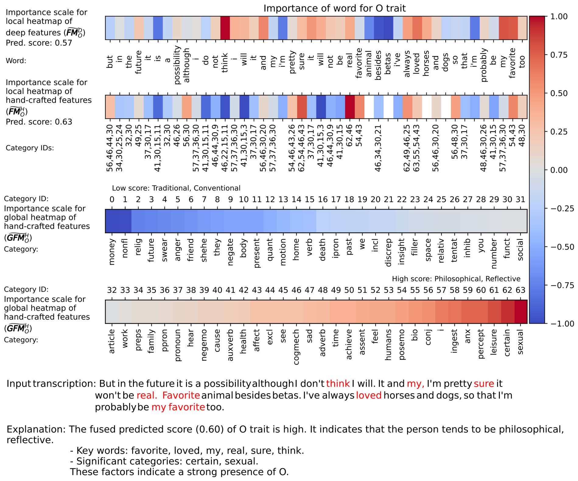
To visualize the heatmaps (importance) of the words and word categories and to explain the model predictions (see Figure 6), we randomly selected one test utterance. The word importance for ${\widetilde{\mathit{FM}}}_O^D$, ${\widetilde{\mathit{FM}}}_O^H$, and ${\widetilde{\mathit{GFM}}}_O^H$ ranges from −1 (blue, the least informative) to 1 (red, the most informative). For the O trait, the most important words are “think”, “real”, “sure”, “favorite”, and “loved”, indicating cognitive engagement, emotional expressiveness, and well-defined preferences.

These behavioral indicators are consistent with O, reflecting intellectual curiosity, self-confidence, and an appreciation of aesthetic and emotional depth. The heatmap for ${\widetilde{\mathit{GFM}}}_O^H$ illustrates word categories with values from −1 to 0 (low scores) and from 0 to 1 (high scores). Since the test utterance contains words from highly predictive categories, such as sexual (“loved”) and certain (“real” and “sure”), the predicted score for ${\widetilde{\mathit{FM}}}_O^H$ is 0.63, which differs from the predicted score for ${\widetilde{\mathit{FM}}}_O^D$ (0.57). After the fusion step, the final score is 0.6, because the model mainly relies on the ${\widetilde{\mathit{FM}}}_O^D$ prediction.

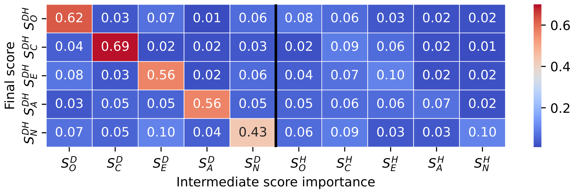
Figure 7 and Figure 8 illustrate how intermediate predictions contribute to the final PT scores in the fusion models trained on FIv2 and PANDORA, respectively. On FIv2, the fusion model primarily relies on predictions based on deep features. The diagonal entries indicate that each trait depends mainly on its own intermediate prediction, with the highest contributions for O ($S_O^{DH}=0.62$) and C ($S_C^{DH}=0.69$). For the remaining traits, the off-diagonal values reveal cross-trait influences. E receives notable input from O ($S_O^D=0.08$) and C ($S_C^H=0.07$). A distributes the weights almost equally across all other PTs. N is moderately influenced by E ($S_E^D=0.10$ and $S_E^H=0.10$) and C ($S_C^H=0.09$). The relatively low off-diagonal values suggest that the final scores are largely trait-specific, with limited interdependence across the OCEAN dimensions.

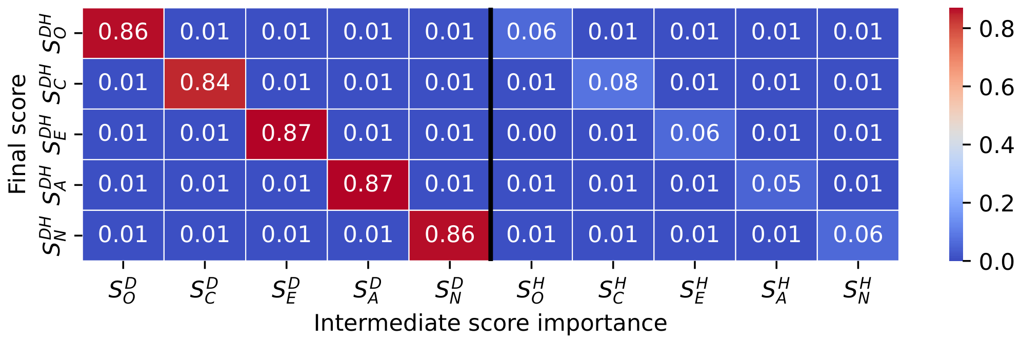
On PANDORA, this pattern is even more pronounced. The mean fusion weights across the five folds show a strong dominance of the diagonal entries, which range from 0.84 to 0.87, whereas most off-diagonal contributions remain close to 0.01. The average contribution of hand-crafted predictions ranges from 0.05 to 0.08, with moderate variability across folds. Compared with FIv2, the fusion models trained on PANDORA are driven more strongly by predictions obtained from deep features and show a weaker reliance on predictions based on hand-crafted features.

6. Discussion

Our experimental evaluation demonstrates the potential of ExPAM. Since automatic PA is intended for real-world human-centered applications, its applicability should also be considered together with possible ethical risks. However, a deeper understanding of its behavior, limitations, and contextual dependencies is needed to fully assess its real-world applicability. In this section, we examine the statistical significance of the improvements achieved by ExPAM, analyze model bias, and investigate prediction errors through illustrative examples. We also explain our choice of LLMs and assess the impact of prompt engineering across zero-shot, one-shot, few-shot, and explanation-based setups. Finally, we further summarize the findings to answer the research questions posed in the introduction and outline methodological limitations and directions for future research.

Overall, ExPAM can support educational personalization, adaptive tutoring, user-aware conversational agents, digital coaching, recommender systems, and human–computer interaction scenarios, where estimated PT may help adapt communication strategies to individual users. At the same time, automatic PA raises ethical concerns related to privacy, informed consent, demographic and corpus-specific biases, and the possible overinterpretation of inferred PTs. Therefore, ExPAM should be considered as a research-oriented and decision-support tool rather than an autonomous system for high-stakes decisions such as hiring, diagnosis, or psychological profiling. Its explainable design partially mitigates these risks by making model decisions more transparent; however, practical deployment would still require human oversight, clear usage policies, and validation in the target application context.

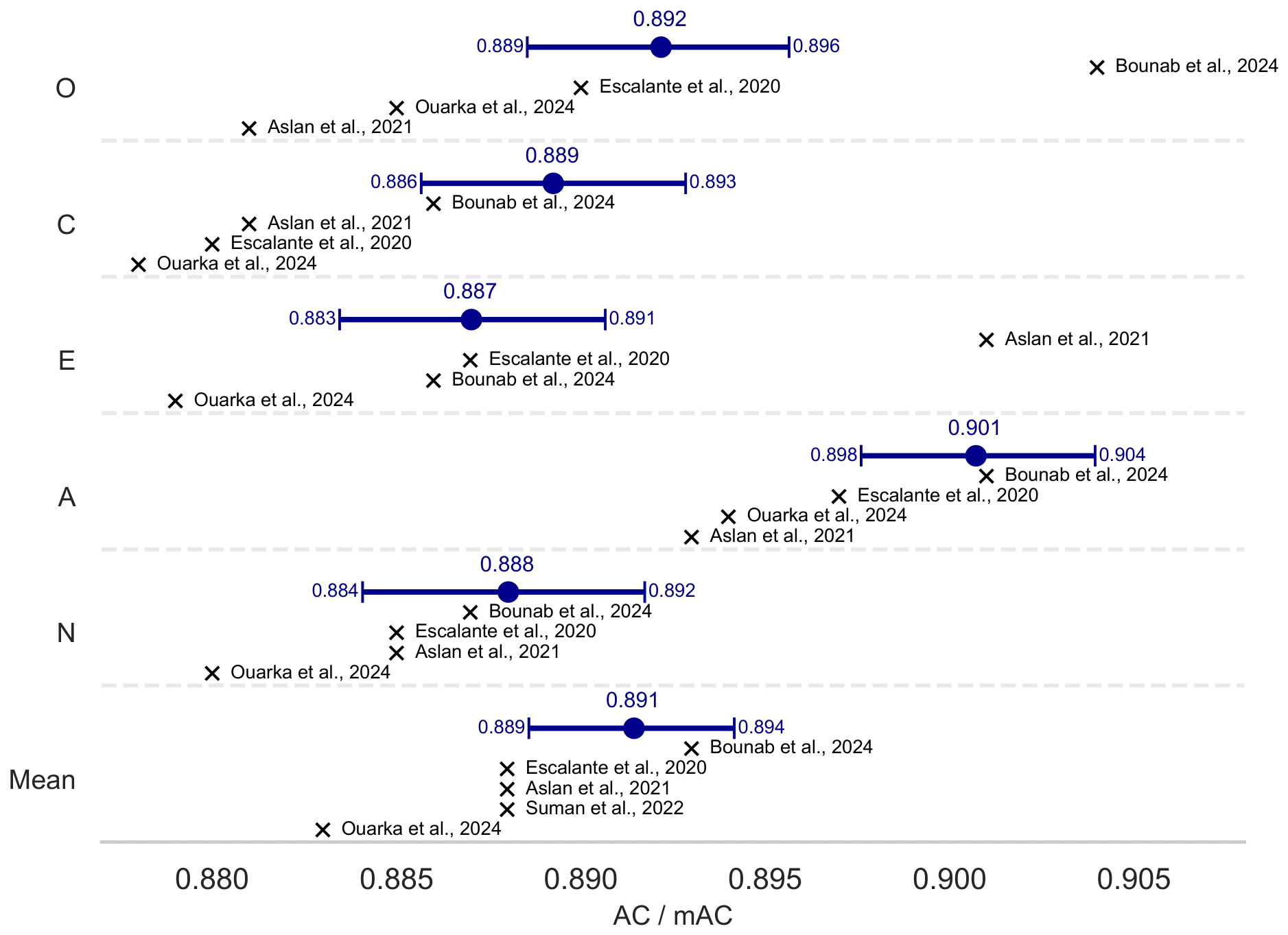
Figure 9 presents a comparison of ExPAM with SOTA methods on the FIv2 corpus across all five PTs and the overall mAC. For ExPAM, 95% confidence intervals are shown as horizontal lines with central markers indicating the estimated performance, while SOTA results are represented by single-point estimates for the same measures. ExPAM demonstrates competitive or superior performance across all PTs, with particularly strong results in C, A, and N, where its confidence interval lies above the SOTA point estimates. However, for the O and E PT, ExPAM is inferior to SOTA [13,34], since the SOTA point estimates exceed the upper bounds of the corresponding confidence intervals. The mAC of ExPAM lies within the upper range of reported SOTA results, highlighting its effectiveness in the PT prediction.

6.1. Statistical Significance of Performance Gains

It should be noted that FIv2 and PANDORA follow different official evaluation protocols. PANDORA provides predefined author-level folds, making it possible to report the mean and standard deviation of the performance measures across the five official folds. In contrast, FIv2 is evaluated using the official fixed Train/Development/Test subsets: the models are trained on the Train subset, the hyperparameters are selected on the Development subset, and the final performance is reported on the Test subset. Therefore, constructing additional folds for FIv2 would modify the standard benchmark protocol and make comparisons with previously published SOTA methods inconsistent.

To assess the statistical reliability of the FIv2 results while preserving the official evaluation protocol, we used a non-parametric bootstrap resampling procedure [61]. Specifically, 1000 bootstrap resamples of the official Test subset were generated by sampling test instances with replacement, such that each resample had the same size as the original Test subset and individual test instances could appear multiple times within a single resample. For each bootstrap replicate, we recomputed AC for each PT and mAC across all five PTs. The 2.5th and 97.5th percentiles of the resulting bootstrap distributions were used as the lower and upper bounds of the 95% confidence intervals. These confidence intervals provide a statistically grounded estimate of the uncertainty of ExPAM performance on the official FIv2 Test subset without redefining the benchmark split.

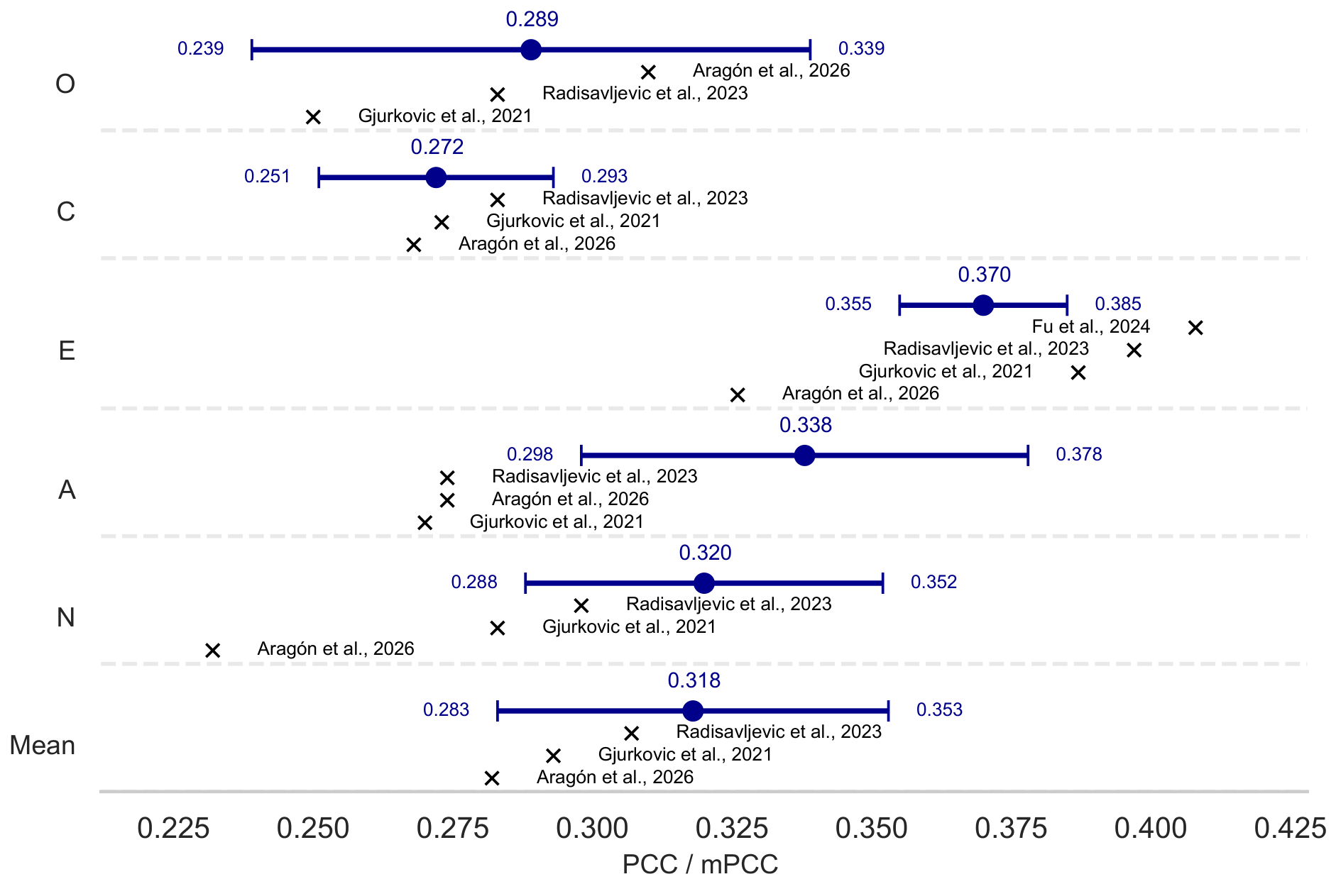
Figure 10 presents the corresponding comparison on PANDORA for the single-task ExPAM. In contrast to FIv2, the variability is estimated as the standard deviation across all five official folds. ExPAM achieves the best mean performance among the compared methods and shows clear advantages for A and N, where its intervals are above the reported SOTA point estimates. For E, ExPAM remains competitive but does not surpass the strongest previous result, while for O and C, it remains below the best single-task baselines. At the same time, ExPAM achieves a higher mean mPCC than all compared methods, indicating that it provides the best overall balance across PTs on PANDORA.

Overall, the results indicate that ExPAM provides competitive mean performance on both FIv2 and PANDORA while preserving a unified formulation for all five PTs. Although some existing SOTA methods achieve better results for individual PTs, ExPAM remains superior at the level of the full OCEAN profile and also shows clear advantages for several PTs.

6.2. Bias Analysis

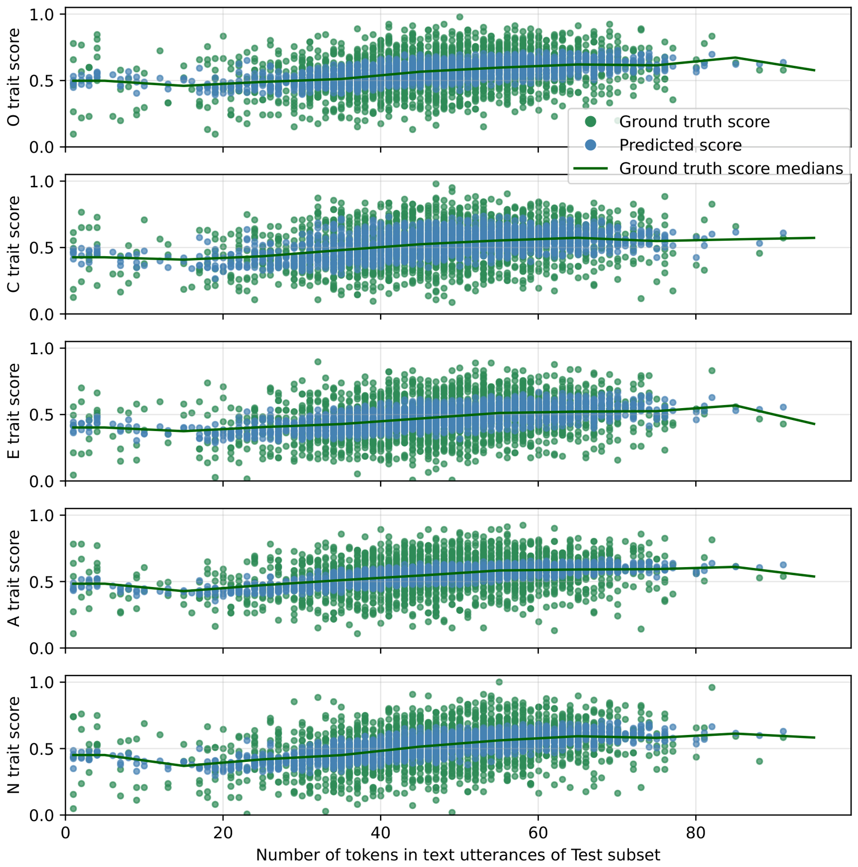
Figure 11 shows the relationship between utterance length, measured in tokens, and both the ground truth and predicted scores for the Big Five PTs. This analysis is feasible for FIv2 because each speaker is represented by a single utterance. In PANDORA, however, each author is associated with multiple comments of varying lengths. The ground truth scores exhibit a consistent positive trend across all PTs: as the number of tokens increases, median scores tend to rise, indicating that longer utterances are systematically assigned higher PTs values. These patterns suggest an inherent length-based annotation bias and further imply that annotation may also rely on non-linguistic data (e.g., audio or video). The model’s predictions also follow this trend, but with lower variability. The predicted scores cluster more tightly around the median than the wider range observed in human annotations, suggesting that the model may underestimate the full range of human judgments. This limitation arises because the training data are concentrated in a certain range, as shown in Figure 1. The ground truth scores fall primarily between 0.4 and 0.6, with fewer examples at the extremes. Consequently, the model lacks sufficient training data for very low or very high PT levels, so it cannot accurately predict extreme values. As a result, the model appears to learn primarily PT polarity (e.g., extroverted vs. introverted), rather than nuanced continuous PT levels. This dependence of both ground truth and predicted scores on utterance length raises concerns about fairness and generalization, highlighting the need to handle input length carefully in PA systems to reduce systematic errors across texts of different lengths.

6.3. Qualitative Error Analysis

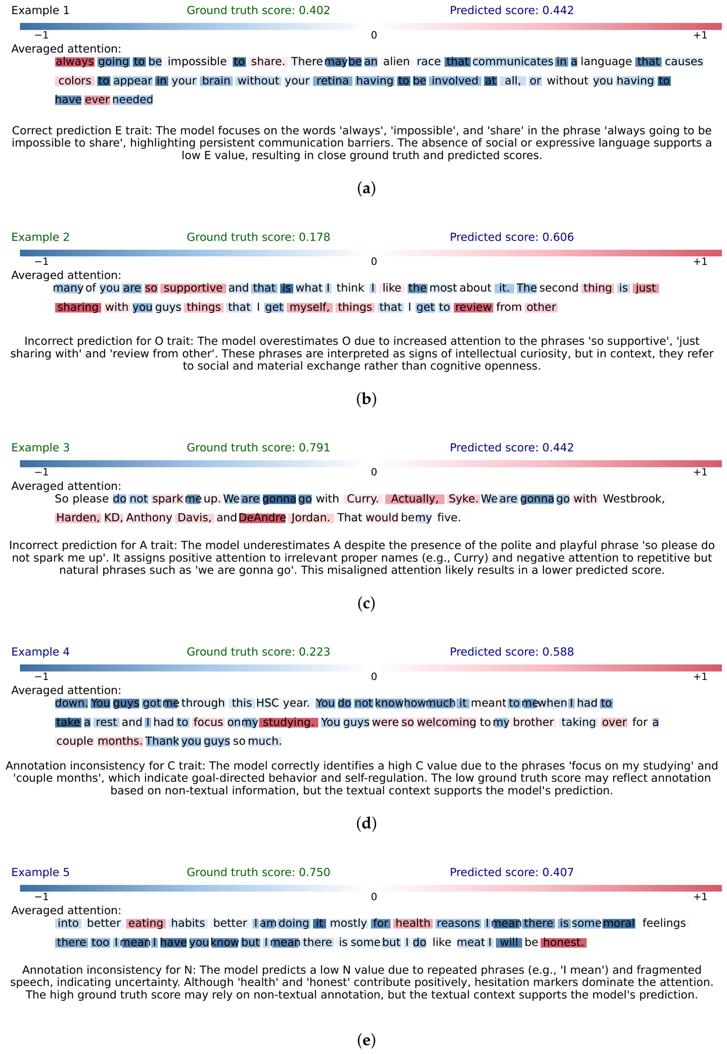
Figure 12 presents a qualitative analysis of the model’s predictions using five representative examples, illustrating the interaction between ground truth scores, predicted scores, and attention patterns. The first example (see Figure 12a) demonstrates strong alignment between the ground truth and predicted scores (both low). The model correctly identifies key linguistic cues (e.g., expressions of social withdrawal and emotional distance) that support a low E score. This suggests that the model can accurately capture relevant patterns when they are clearly expressed in the text.

The second and third examples (see Figure 12b and Figure 12c, respectively) highlight model errors arising from misaligned attention. In Example 2, the model overestimates O, assigning high attention to phrases such as “so supportive”, “just sharing with”, and “review from other” and interpreting them as signs of intellectual curiosity. However, these phrases refer to social and material exchange rather than cognitive openness. In Example 3, despite a high ground truth score for A, the model underestimates the score, overlooking the polite phrase “so please do not spark me up”. Instead, it focuses on neutral proper names (e.g., Curry, Westbrook) and repetitive phrasing (e.g., “we are gonna go”), which together lack trait-relevant meaning. This reflects a tendency to prioritize surface-level tokens over contextually grounded linguistic signals.

The last two examples reveal potential issues in the annotation process. In Example 4 (see Figure 12d), the model predicts a high score based on clear indicators of Conscientiousness (e.g., “focus on my studying” and “couple months”), yet the ground truth score is low. Similarly, in Example 5 (see Figure 12e), the model predicts a low N score, driven by attention to hesitation markers such as “I mean” and fragmented phrasing, which typically signal uncertainty and thus support a low N prediction; however, the ground truth score is high. These discrepancies suggest that the annotations may not fully reflect the textual content and may instead rely on non-linguistic features (e.g., acoustic or visual). Thus, these cases point to annotation errors, where human estimates deviate from the evidence present in the text.

Overall, the analysis shows that the model’s predictions fall into either correct or incorrect outcomes. In the latter case, errors arise either from model limitations, such as misprioritizing linguistic features, or from annotation inconsistencies, where ground truth scores do not align with textual evidence. This distinction underscores the importance of evaluating both model performance and data quality in PA, particularly when interpreting results in real-world applications.

6.4. LLM Integration and Prompt Engineering

Table 6. Comparison of LLM characteristics. Inference time is reported for 2K test requests.

Model	Release	Link	Parameters/Layers	Architecture	Training Data	Inference, min
Qwen3.5-4B	March 2026	HF	4B/32	Hybrid: Gated DeltaNet + Gated Attention, CLM with vision encoder	Supports 201 languages and dialects	≈60
Qwen3.5-9B	March 2026	HF	9B/32	Hybrid: Gated DeltaNet + Gated Attention, CLM with vision encoder	Supports 201 languages and dialects	≈80
Qwen3.5-27B	March 2026	HF	27B/64	Hybrid: Gated DeltaNet + Gated Attention, CLM with vision encoder	Supports 201 languages and dialects	≈130
Qwen3.5-35B	March 2026	HF	35B, 3B active/40	Hybrid: Gated DeltaNet + Gated Attention with sparse MoE, CLM with vision encoder	Supports 201 languages and dialects	≈150
Qwen3.6-35B	April 2026	HF	35B, 3B active/40	Hybrid: Gated DeltaNet + Gated Attention with sparse MoE, CLM with vision encoder	Supports 201 languages and dialects	≈120
Gemma4-E4B	April 2026	HF	8B, 4.5B effective/42	Hybrid attention: local sliding-window + full global attention, p-RoPE; PLE	Large-scale pre-training data including web documents, code, images, and audio; content in 140+ languages	≈110
Gemma4-31B	April 2026	HF	30.7B/60	Hybrid attention: local sliding-window + full global attention, p-RoPE	Large-scale pre-training data including web documents, code, images, and audio; content in 140+ languages	≈140
Falcon-H1-7B	July 2025	HF	7B/44	Causal decoder-only; Hybrid Transformers + Mamba architecture	English, multilingual	≈150
Falcon-H1-34B	July 2025	HF	34B/72	Causal decoder-only; Hybrid Transformers + Mamba architecture	English, multilingual	≈200
GigaChat3-10B	December 2025	HF	10B, 1.8B active/26	Custom MoE with MLA and MTP	20T tokens; 10 added languages; books, academic data, code and math datasets; about 5.5T synthetic tokens	≈110
GLM4.7-31B	August 2025	HF	31B, 3B active/47	Sparse MoE, CLM decoder-only	Not predestined	≈80

summarizes the characteristics of the LLMs used in our experiments. We selected open-weight models from the Qwen, Gemma, Falcon, GigaChat, and GLM families, covering a wide range of parameter scales and architectural designs, including hybrid attention-based models, Mixture of Experts (MoE) variants, and Transformer + Mamba hybrids. We used only publicly available models because their released weights ensure reproducible inference and avoid dependence on proprietary API-based systems such as ChatGPT, DeepSeek, and other commercial LLMs. We also tested GPT-OSS-20B (https://huggingface.co/openai/gpt-oss-20b, accessed on 13 July 2026), but excluded it from Table 6 and the final comparison because, under our compact instructions, it did not produce the required numeric outputs.

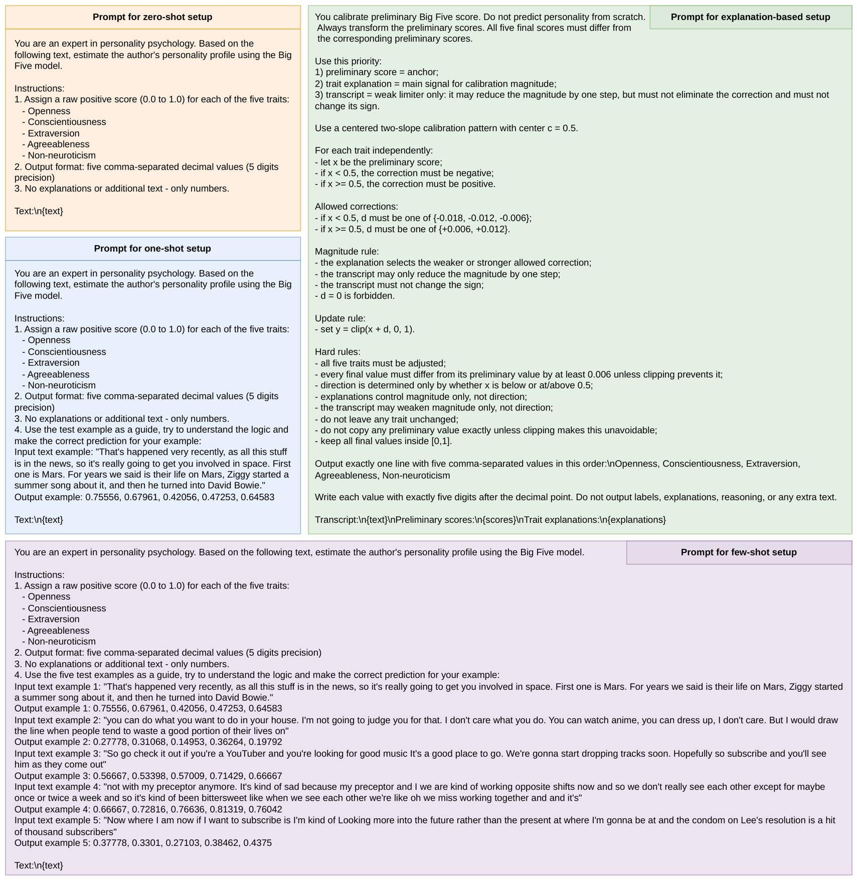
The selection of prompts is an important step in testing LLMs. Figure 13 presents the prompts that show the highest average performance across all models. However, it should be noted that some models performed better with certain prompts, while others excelled on different ones. Since the goal of this work is not to optimize the LLM performance, but to demonstrate their ability in PA without fine-tuning for a specific task, we limit our analysis to the most effective prompts.

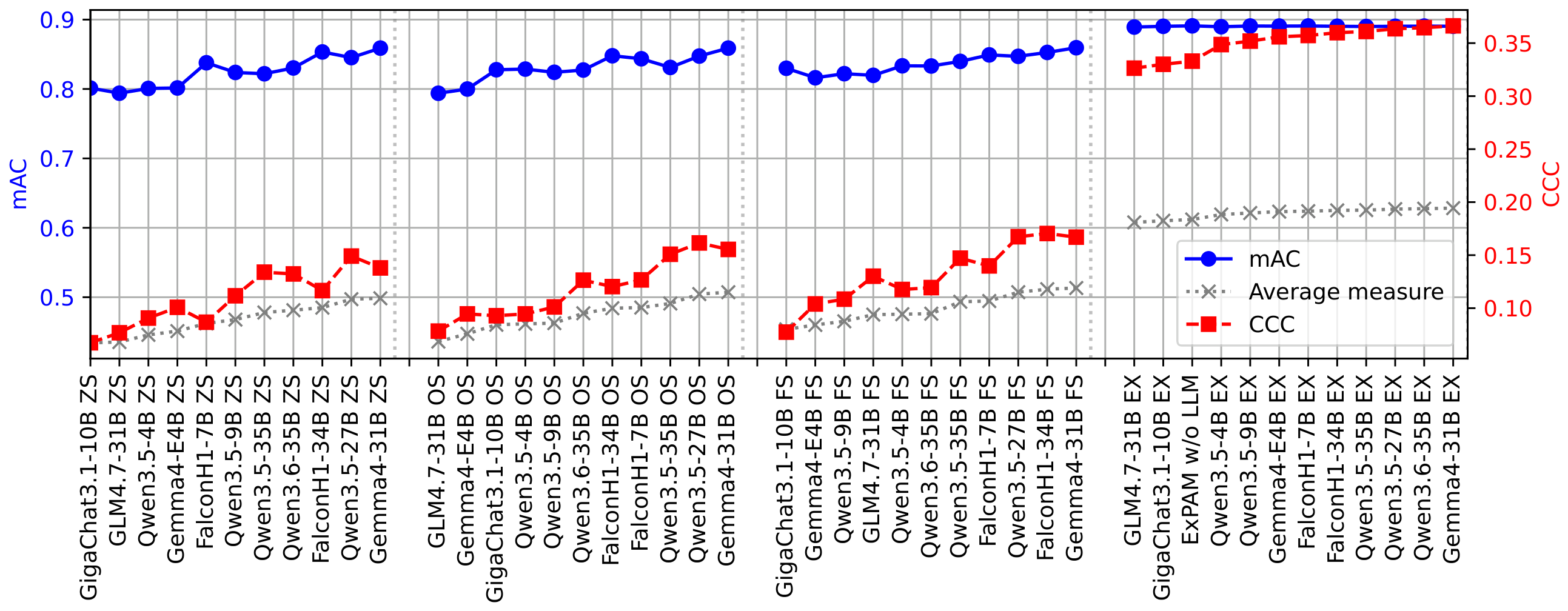
Experimental results on the FIv2 corpus (see Figure 14) indicate that the prompting strategy has a substantial impact on the performance of off-the-shelf LLMs. While one-shot and few-shot prompting generally improve performance compared with the zero-shot setup, the best results are achieved with explanation-based prompting. In this setting, both CCC and the average of CCC and mAC show a marked increase, whereas mAC remains high and stable across model families. In terms of a model scale, larger LLMs do not offer a decisive advantage over medium-scale models. Although some of the strongest results are achieved by larger models, medium-scale models already reach highly competitive performance, especially in the explanation-based setup, where the gap between medium and large models becomes relatively small. This suggests that explanation-based prompting plays a more important role than model scale alone and that medium-scale open-weight models may provide a better trade-off between both a predictive quality and a computational efficiency.

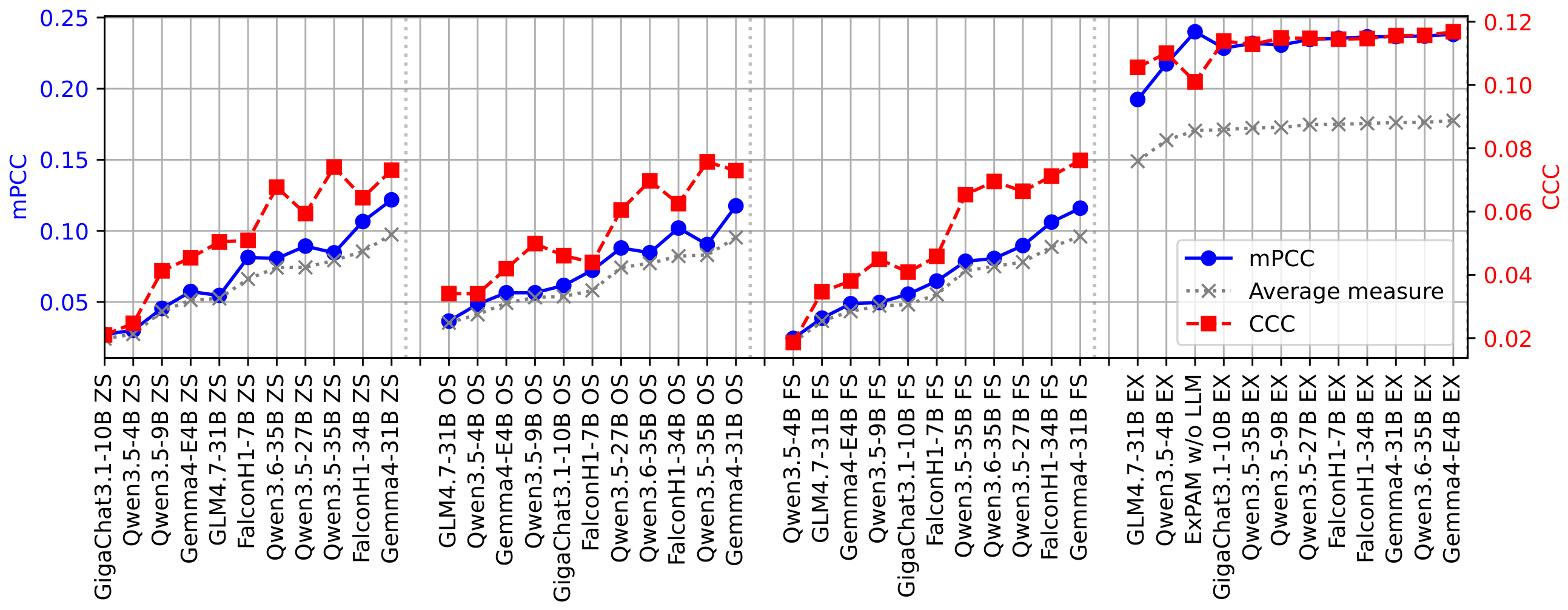
Experimental results on the PANDORA corpus (see Figure 15) are generally consistent with those on FIv2. In particular, explanation-based prompting again provides the best overall performance, confirming that LLMs benefit most from structured explanations produced by the proposed method. At the same time, unlike on FIv2, one-shot and few-shot prompting do not yield consistent improvements over the zero-shot setup, suggesting greater variability and structural complexity of utterances in PANDORA. In addition, larger models do not demonstrate a clear advantage: under explanation-based prompting, the lighter Gemma4-E4B achieves the best result, indicating that a model size itself does not determine a high efficiency. Overall, these findings confirm that LLMs are most effective when used together with explanations rather than as standalone predictors.

Overall, the results on both FIv2 and PANDORA show that the explanation-based prompting is the most reliable strategy for integrating LLMs. While zero-shot, one-shot, and few-shot setups are more corpus-dependent, structured explanations improve the effectiveness of LLM-based PA.

6.5. Responses to Research Questions

RQ1: Can hybrid fusion that combines hand-crafted and deep linguistic features improve both prediction performance and interpretability in PA?

Our results are summarized in Table 1 and Table 2. On FIv2, the fusion of deep features (ID 6: XLM-RoBERTa + ReBiLSTM-Att) with hand-crafted features (ID 14: LIWC + ReBiLSTM-Att) yields only a modest change in mAC but improves CCC: the combined model (ID 17) achieves a CCC of 0.333, corresponding to a 7.1% relative improvement over the best single-feature model (ID 6, $\mathrm{CCC}=0.311$). On PANDORA, the same fusion strategy also improves performance: the combined model (ID 17) reaches $\mathrm{mPCC}=0.240$ and $\mathrm{CCC}=0.101$, compared with $\mathrm{mPCC}=0.238$ and $\mathrm{CCC}=0.093$ for the best model based on deep features (ID 6), corresponding to relative gains of 0.8% and 8.6%, respectively. These results show that the fusion of deep and hand-crafted features improves the robustness of the proposed method across both corpora.

In addition, this hybrid design preserves and improves interpretability. Deep features capture token-level contextual evidence, whereas LIWC provides psychologically grounded category-level evidence. At the same time, Figure 7 illustrates how the fusion weights predominantly rely on deep-feature predictions, particularly for Openness and Conscientiousness, while still using hand-crafted features when they are linguistically informative (e.g., for Agreeableness and Neuroticism). Overall, the hybrid fusion offers a useful trade-off: it preserves competitive predictive performance while providing more transparent explanations.

RQ2: Can gradient-based interpretation be adapted to textual data to explain PT predictions through token-level and LIWC-category-level evidence?

Our findings confirm that gradient-based interpretation methods originally developed for visual models, such as Grad-CAM, can be successfully adapted to text data. By computing the gradient of each trait-specific output with respect to the input feature matrices, both deep and hand-crafted, we generate token- and category-level importance heatmaps (see Section 4.2). As shown in Figure 6, these heatmaps reveal linguistically coherent and psychologically meaningful patterns. For example, words such as “think”, “loved”, and “sure” emerge as strong indicators of high Openness, which is consistent with theoretical expectations regarding cognitive engagement and emotional expressiveness. At the category-level, the global heatmap highlights trait-relevant LIWC categories (e.g., “certain” and “sexual”) across the Train subset. Overall, our results suggest that vision-inspired interpretability methods, when applied to the sequential and categorical structure of linguistic features in PA, can produce useful and theory-aligned explanations.

RQ3: Can explanations generated by the proposed model effectively serve as in-context prompts for LLMs to improve PT prediction performance without any fine-tuning?

Empirical results support this claim on both corpora. On FIv2 (see Table 1), when ExPAM fused scores and trait-specific explanations are used as prompts in the explanation-based in-context learning setup, the best LLM-based configuration (ID 21) achieves $\mathrm{CCC}=0.366$, compared with $\mathrm{CCC}=0.333$ for the hybrid ExPAM model without LLM integration (ID 17), corresponding to a relative improvement of 9.9%. At the same time, mAC remains nearly unchanged (0.890 vs. 0.891). Moreover, compared with the best few-shot setup (ID 20, $\mathrm{CCC}=0.167$), the explanation-based configuration more than doubles the CCC value, highlighting the importance of explanation-enriched prompting over standard in-context examples alone.

A similar pattern is observed on PANDORA (see Table 2). The explanation-based setup (ID 21) improves CCC from 0.101 to 0.117 relative to the fused ExPAM model without LLM integration, yielding a 15.8% relative gain, while mPCC changes only marginally, from 0.240 to 0.238. Compared with the best few-shot setup (ID 20, $\mathrm{CCC}=0.076$), the explanation-based prompting yields a 53.9% relative improvement in CCC. These results suggest that the observed CCC improvement is not determined by model size alone and may be related to the structured trait-level rationales generated by ExPAM.

The zero-shot, one-shot, and few-shot setups evaluate LLM-based PA without ExPAM-derived explanations and without constrained calibration of preliminary scores. In contrast, the explanation-based setup is formulated as a constrained score calibration procedure: the preliminary ExPAM scores are used as anchors, the prompt defines the allowed direction and magnitude of score changes, and the trait-specific explanations guide the correction magnitude. Therefore, the gain should be attributed to the complete explanation-guided calibration procedure rather than to unconstrained LLM reasoning or to the explanations alone.

Overall, ExPAM-generated explanations serve as effective in-context prompts, connecting interpretable intermediate predictions with the reasoning capabilities of off-the-shelf LLMs.

7. Limitations and Future Work

ExPAM has several non-critical limitations for explainable Big Five PA. First, although we evaluate the proposed method on two corpora with substantially different properties, namely FIv2 and PANDORA, both corpora still represent restricted experimental settings. FIv2 consists of short 15-second monologues and therefore does not fully reflect natural conversational dynamics, while PANDORA is based on author-level Reddit comments and captures a written language rather than a spoken one. As a result, the current evaluation does not yet cover longer, multi-turn, and fully naturalistic conversational scenarios. Second, the English-only LIWC dictionary limits a cross-lingual applicability. Extending the method to other languages would require multilingual LIWC resources or comparable psycholinguistic lexicons. Third, although we explored open-weight LLMs across a range of scales, from compact 4B models to large models with 35B to 37B parameters, their integration still substantially increases computational costs. For 2K test instances, inference time rises from about 12 min for ExPAM without LLMs to roughly 60–200 min, depending on the selected model, which currently limits a real-time deployment. Finally, the ground truth labels in both corpora differ in nature: FIv2 relies on observer ratings, whereas PANDORA uses author-level trait annotations obtained from social media data. These differences may introduce corpus-specific biases and reduce the comparability of absolute performance values across datasets.

Another limitation is that the numerical gains in the main performance measures are modest; therefore, ExPAM should not be interpreted as providing a large improvement over SOTA methods, but rather as a competitive and interpretable profile-level PA method. In addition, the generated explanations were analyzed qualitatively and were not evaluated by independent psychology experts; therefore, their psychological validity should be further examined in a dedicated expert-based study. Finally, although the multi-task configuration is more scalable for the simultaneous prediction and explanation of all five PTs, it may underperform stronger single-task models on some corpora, especially when the goal is to maximize trait-wise predictive accuracy.

Future work will address these limitations by extending the evaluation beyond short monologues and written author-level comments to longer, multi-turn, and more naturalistic interaction settings, as well as by assessing robustness under stronger domain and distribution shifts. To improve cross-lingual applicability, we will include multilingual psycholinguistic lexicons, such as LIWC resources for additional languages and study transfer across languages. To reduce the computational overhead introduced by LLMs, we will investigate efficiency-focused designs such as distilled models, batching and caching strategies, and more compact prompts, aiming to move toward near real-time inference. Finally, we will examine how different label sources (observer ratings vs. standardized self-reports) influence bias and reliability. Future work will also include expert-based assessment of explanation plausibility and a more detailed analysis of the trade-off between a single-task accuracy and a multi-task scalability.

8. Conclusions

This work introduces ExPAM, a hybrid explainable linguistic method for Big Five PA from text. ExPAM combines LIWC-based hand-crafted psycholinguistic features with deep word representations extracted using XLM-RoBERTa. The best-performing configuration uses ReBiLSTM-Att for both feature types and combines their intermediate predictions through an FCL-based weighted fusion. In addition, attention outputs and gradient-based importance scores are used to build interpretable heatmaps over words, tokens, and LIWC categories. These explanations, together with fused predicted scores, are used as prompts for off-the-shelf LLMs in the explanation-based calibration setup.

Our experiments on both FIv2 and PANDORA show that ExPAM provides competitive PA performance even without integration with LLMs. On FIv2, ExPAM exceeds previously reported multi-task SOTA methods in mAC, reaching $\mathrm{mAC}=0.891$ and $\mathrm{CCC}=0.333$. On PANDORA, ExPAM provides a multi-task baseline with $\mathrm{mPCC}=0.240$ and $\mathrm{CCC}=0.101$, while its single-task variant achieves stronger results. Among the prompting strategies evaluated with the considered open-weight LLMs, the explanation-based setup produced the highest CCC on both corpora, with $\mathrm{CCC}=0.366$ on FIv2 and $\mathrm{CCC}=0.117$ on PANDORA.

Thus, the main contribution of ExPAM lies in combining competitive prediction quality with interpretable trait-specific explanations, which is important for applications, where understanding the reasons behind the predictions is crucial. The source code is publicly available at https://github.com/SMIL-SPCRAS/ExPAM (accessed on 13 July 2026).

References

1. Ryumina, E.; Markitantov, M.; Ryumin, D.; Karpov, A. OCEAN-AI framework with EmoFormer cross-hemiface attention approach for personality traits assessment. Expert Syst. Appl. 2024, 239, 122441. [Google Scholar] [CrossRef] [Scilit]
2. McCrae, R.R.; John, O.P. An introduction to the five-factor model and its applications. J. Personal. 1992, 60, 175–215. [Google Scholar] [CrossRef] [Scilit] [PubMed]
3. Nikčević, A.V.; Marino, C.; Kolubinski, D.C.; Leach, D.; Spada, M.M. Modelling the contribution of the Big Five personality traits, health anxiety, and COVID-19 psychological distress to generalised anxiety and depressive symptoms during the COVID-19 pandemic. J. Affect. Disord. 2021, 279, 578–584. [Google Scholar] [CrossRef] [Scilit] [PubMed]
4. Liu, Z.; Yin, S.X.; Lin, G.; Chen, N.F. Personality-aware Student Simulation for Conversational Intelligent Tutoring Systems. In Proceedings of the Conference on Empirical Methods in Natural Language Processing (EMNLP), Miami, FL, USA, 12–16 November 2024; pp. 626–642. [Google Scholar] [CrossRef] [Scilit]
5. Naz, A.; Khan, H.U.; Alsahfi, T.; Alhajlah, M.; Alshemaimri, B.; Daud, A. Using transformers and Bi-LSTM with sentence embeddings for prediction of openness human personality trait. PeerJ Comput. Sci. 2025, 11, e2781. [Google Scholar] [CrossRef] [Scilit] [PubMed]
6. Thapa, L.; Pandey, A.; Gupta, D.; Deep, A.; Garg, R. A Framework for Personality Prediction for E-Recruitment Using Machine Learning Algorithms. In Proceedings of the 14th International Conference on Cloud Computing, Data Science & Engineering (Confluence), Noida, India, 14–15 January 2024; pp. 1–5. [Google Scholar] [CrossRef] [Scilit]
7. Ryumina, E.; Ryumin, D.; Karpov, A. OCEAN-AI: Open multimodal framework for personality traits assessment and HR-processes automatization. In Proceedings of the Interspeech, Kos, Greece, 1–5 September 2024; pp. 1–2. [Google Scholar]
8. Valovy, M.; Buchalcevova, A. Personality-based pair programming: Toward intrinsic motivation alignment in very small entities. PeerJ Comput. Sci. 2025, 11, e2774. [Google Scholar] [CrossRef] [Scilit] [PubMed]
9. Ryumina, E.; Markitantov, M.; Ryumin, D.; Karpov, A. Gated Siamese Fusion Network based on multimodal deep and hand-crafted features for personality traits assessment. Pattern Recognit. Lett. 2024, 185, 45–51. [Google Scholar] [CrossRef] [Scilit]
10. Ryumina, E.; Axyonov, A.; Koryakovskaya, D.; Abdulkadirov, T.; Egorova, A.; Fedchin, S.; Zaburdaev, A.; Ryumin, D. SSL-MEPR: A Semi-Supervised Multi-Task Cross-Domain Learning Framework for Multimodal Emotion and Personality Recognition. Mach. Learn. Knowl. Extr. 2026, 8, 56. [Google Scholar] [CrossRef] [Scilit]
11. Panfilova, A.S.; Turdakov, D.Y. Applying explainable artificial intelligence methods to models for diagnosing personal traits and cognitive abilities by social network data. Sci. Rep. 2024, 14, 5369. [Google Scholar] [CrossRef] [Scilit] [PubMed]
12. Ryumina, E.; Axyonov, A.; Abdulkadirov, T.; Koryakovskaya, D.; Ryumin, D. Cross-Lingual Bimodal Emotion Recognition with LLM-Based Label Smoothing. Big Data Cogn. Comput. 2025, 9, 285. [Google Scholar] [CrossRef] [Scilit]
13. Bounab, Y.; Oussalah, M.; Arhab, N.; Bekhouche, S. Towards job screening and personality traits estimation from video transcriptions. Expert Syst. Appl. 2024, 238, 122016. [Google Scholar] [CrossRef] [Scilit]
14. Pennebaker, J.W.; Boyd, R.L.; Jordan, K.; Blackburn, K. The Development and Psychometric Properties of LIWC2015; University of Texas at Austin: Austin, TX, USA, 2015; p. 407. [Google Scholar] [CrossRef] [Scilit]
15. Jiang, Z.; Zheng, X.; Yu, W.; Chen, J. Exploring the effects of personality traits on customer perceived value based on text decomposition. IEEE Access 2025, 13, 62137–62153. [Google Scholar] [CrossRef] [Scilit]
16. Han, W.; Chen, Y.; Xing, X.; Zhou, G.; Xu, X. Speaker-aware hierarchical transformer for personality recognition in multiparty dialogues. In Proceedings of the International Conference on Acoustics, Speech and Signal Processing (ICASSP), Rhodes Island, Greece, 4–10 June 2023; pp. 1–5. [Google Scholar] [CrossRef] [Scilit]
17. Yang, F.; Yang, T.; Quan, X.; Su, Q. Learning to answer psychological questionnaire for personality detection. In Proceedings of the Findings of the Association for Computational Linguistics: EMNLP, Punta Cana, Dominican Republic, 7–11 November 2021; pp. 1131–1142. [Google Scholar] [CrossRef] [Scilit]
18. Wang, R.; Xu, X.; Yang, H.; Wei, L.; Ma, H. A novel multimodal personality prediction method based on pretrained models and graph relational transformer network. In Proceedings of the International Conference on Acoustics, Speech and Signal Processing (ICASSP), Hyderabad, India, 6–11 April 2025; pp. 1–5. [Google Scholar] [CrossRef] [Scilit]
19. Müller, O.; Degaetano-Ortlieb, S. Embedded Personalities: Word Embeddings and the “Big Five” Personality Model. In Proceedings of the Joint SIGHUM Workshop on Computational Linguistics for Cultural Heritage, Social Sciences, Humanities and Literature (LaTeCH-CLfL), Albuquerque, NM, USA, 4 May 2025; pp. 205–215. [Google Scholar] [CrossRef] [Scilit]
20. Sun, L.; Zhao, J.; Jin, Q. Revealing Personality Traits: A New Benchmark Dataset for Explainable Personality Recognition on Dialogues. In Proceedings of the Conference on Empirical Methods in Natural Language Processing (EMNLP), Miami, FL, USA, 12–16 November 2024; pp. 19988–20002. [Google Scholar] [CrossRef] [Scilit]
21. Wen, Z.; Cao, J.; Yang, Y.; Yang, R.; Liu, S. Affective-NLI: Towards accurate and interpretable personality recognition in conversation. In Proceedings of the International Conference on Pervasive Computing and Communications (PerCom), Biarritz, France, 11–15 March 2024; pp. 184–193. [Google Scholar] [CrossRef] [Scilit]
22. Maharjan, J.; Jin, R.; Zhu, J.; Kenne, D. Psychometric Evaluation of Large Language Model Embeddings for Personality Trait Prediction. J. Med. Internet Res. 2025, 27, e75347. [Google Scholar] [CrossRef] [Scilit] [PubMed]
23. Li, J.; He, Y.; Xu, J.; Luo, T.; Hu, Z.; Hong, R.; Wang, M. Traits Run Deep: Enhancing Personality Assessment via Psychology-Guided LLM Representations and Multimodal Apparent Behaviors. arXiv 2025, arXiv:2507.22367. [Google Scholar] [CrossRef] [Scilit]
24. Park, C.F.; Lee, A.; Lubana, E.S.; Yang, Y.; Okawa, M.; Nishi, K.; Wattenberg, M.; Tanaka, H. ICLR: In-Context Learning of Representations. In Proceedings of the International Conference on Learning Representations (ICLR), Singapore, 24–28 April 2025; pp. 1–27. [Google Scholar]
25. Wu, S.; Wang, Y.; Yao, Q. Why In-Context Learning Models are Good Few-Shot Learners? In Proceedings of the International Conference on Learning Representations (ICLR), Singapore, 24–28 April 2025; pp. 1–13. [Google Scholar]
26. Sandhan, J.; Cheng, F.; Sandhan, T.; Murawaki, Y. CAPE: Context-Aware Personality Evaluation Framework for Large Language Models. arXiv 2025, arXiv:2508.20385. [Google Scholar] [CrossRef] [Scilit]
27. Handa, G.; Wu, Z.; Koshiyama, A.; Treleaven, P. Personality as a Probe for LLM Evaluation: Method Trade-offs and Downstream Effects. arXiv 2025, arXiv:2509.04794. [Google Scholar] [CrossRef] [Scilit]
28. Gu, A.; Dao, T. Mamba: Linear-time sequence modeling with selective state spaces. arXiv 2023, arXiv:2312.00752. [Google Scholar] [CrossRef] [Scilit]
29. Devlin, J.; Chang, M.W.; Lee, K.; Toutanova, K. Bert: Pre-training of deep bidirectional transformers for language understanding. In Proceedings of the Conference of the North American Chapter of the Association for Computational Linguistics: Human Language Technologies, Volume 1 (Long and Short Papers), Minneapolis, MN, USA, 2–7 June 2019; pp. 4171–4186. [Google Scholar] [CrossRef] [Scilit]
30. Conneau, A.; Khandelwal, K.; Goyal, N.; Chaudhary, V.; Wenzek, G.; Guzmán, F.; Grave, E.; Ott, M.; Zettlemoyer, L.; Stoyanov, V. Unsupervised Cross-lingual Representation Learning at Scale. In Proceedings of the Annual Meeting of the Association for Computational Linguistics (ACL), Florence, Italy, 28 July–2 August 2019; pp. 8440–8451. [Google Scholar] [CrossRef] [Scilit]
31. Sturua, S.; Mohr, I.; Akram, M.K.; Günther, M.; Wang, B.; Krimmel, M.; Wang, F.; Mastrapas, G.; Koukounas, A.; Wang, N.; et al. jina-embeddings-v3: Multilingual embeddings with task lora. arXiv 2024, arXiv:2409.10173. [Google Scholar] [CrossRef] [Scilit]
32. Escalante, H.J.; Guyon, I.; Escalera, S.; Jacques, J.; Madadi, M.; Baró, X.; Ayache, S.; Viegas, E.; Güçlütürk, Y.; Güçlü, U.; et al. Design of an explainable machine learning challenge for video interviews. In Proceedings of the International Joint Conference on Neural Networks (IJCNN), Anchorage, AK, USA, 14–19 May 2017; pp. 3688–3695. [Google Scholar] [CrossRef] [Scilit]
33. Escalante, H.J.; Kaya, H.; Salah, A.A.; Escalera, S.; Güçlütürk, Y.; Güçlü, U.; Baró, X.; Guyon, I.; Junior, J.C.S.J.; Madadi, M.; et al. Modeling, recognizing, and explaining apparent personality from videos. IEEE Trans. Affect. Comput. 2020, 13, 894–911. [Google Scholar] [CrossRef] [Scilit]
34. Aslan, S.; Güdükbay, U.; Dibeklioğlu, H. Multimodal assessment of apparent personality using feature attention and error consistency constraint. Image Vis. Comput. 2021, 110, 104163. [Google Scholar] [CrossRef] [Scilit]
35. Suman, C.; Saha, S.; Gupta, A.; Pandey, S.K.; Bhattacharyya, P. A multi-modal personality prediction system. Knowl.-Based Syst. 2022, 236, 107715. [Google Scholar] [CrossRef] [Scilit]
36. Ouarka, A.; Ait Baha, T.; Es-Saady, Y.; El Hajji, M. A deep multimodal fusion method for personality traits prediction. Multimed. Tools Appl. 2024, 84, 29665–29687. [Google Scholar] [CrossRef] [Scilit]
37. Revathi, S.; Nagaraja, G.; Azam, F. Deep cross-modal integration with hierarchical multi-head attention for big five personality prediction. Multimed. Tools Appl. 2025, 84, 46833–46862. [Google Scholar] [CrossRef] [Scilit]
38. Radford, A.; Kim, J.W.; Hallacy, C.; Ramesh, A.; Goh, G.; Agarwal, S.; Sastry, G.; Askell, A.; Mishkin, P.; Clark, J.; et al. Learning transferable visual models from natural language supervision. In Proceedings of the International Conference on Machine Learning (ICML), Vienna, Austria, 18–24 July 2021; pp. 8748–8763. [Google Scholar]
39. Gjurković, M.; Karan, V.M.; Vukojević, I.; Bošnjak, M.; Snajder, J. PANDORA Talks: Personality and Demographics on Reddit. In Proceedings of the International Workshop on Natural Language Processing for Social Media, Online, 10 June 2021; pp. 138–152. [Google Scholar] [CrossRef] [Scilit]
40. Radisavljević, D.; Rzepka, R.; Araki, K. Personality types and traits—Examining and leveraging the relationship between different personality models for mutual prediction. Appl. Sci. 2023, 13, 4506. [Google Scholar] [CrossRef] [Scilit]
41. Fu, Y.; Chu, C.; Kawahara, T. StyEmp: Stylizing empathetic response generation via multi-grained prefix encoder and personality reinforcement. In Proceedings of the 25th Annual Meeting of the Special Interest Group on Discourse and Dialogue, Kyoto, Japan, 18–20 September 2024; pp. 172–185. [Google Scholar] [CrossRef] [Scilit]
42. Killian, J., Jr.; Sun, R. Detecting big-5 personality dimensions from text based on large language models. In Proceedings of the International Conference on Deep Learning Theory and Applications, Dijon, France, 10–11 July 2024; Springer: Berlin/Heidelberg, Germany, 2024; pp. 264–278. [Google Scholar] [CrossRef] [Scilit]
43. Wang, R.; Sun, K. Continuous output personality detection models via mixed strategy training. arXiv 2024, arXiv:2406.16223. [Google Scholar] [CrossRef] [Scilit]
44. Shum, K.M.; Ptaszynski, M.; Masui, F. Big five personality trait prediction based on user comments. Information 2025, 16, 418. [Google Scholar] [CrossRef] [Scilit]
45. Shen, L.; Cai, X.; Long, Y.; Razzak, I.; Chen, G.; Jameel, S. EmoPerso: Enhancing personality detection with self-supervised emotion-aware modelling. In Proceedings of the 34th ACM International Conference on Information and Knowledge Management, Seoul, Republic of Korea, 10–14 November 2025; pp. 2577–2587. [Google Scholar] [CrossRef] [Scilit]
46. Aragón, M.E.; Fernandez-Pichel, M.; Losada, D.E. Personality Traits and Demographics Analysis in Online Mental Health Discourse. IEEE Trans. Affect. Comput. 2026, 17, 1940–1951. [Google Scholar] [CrossRef] [Scilit]
47. Chiaburu, T.; Haußer, F.; Bießmann, F. Uncertainty in XAI: Human Perception and Modeling Approaches. Mach. Learn. Knowl. Extr. 2024, 6, 1170–1192. [Google Scholar] [CrossRef] [Scilit]
48. Ribeiro, M.T.; Singh, S.; Guestrin, C. “Why should I trust you?” Explaining the predictions of any classifier. In Proceedings of the ACM SIGKDD International Conference on Knowledge Discovery and Data Mining, San Francisco, CA, USA, 13–17 August 2016; pp. 1135–1144. [Google Scholar] [CrossRef] [Scilit]
49. Lundberg, S.M.; Lee, S.I. A unified approach to interpreting model predictions. In Proceedings of the Conference on Neural Information Processing Systems (NIPS), Long Beach, CA, USA, 4–9 December 2017; pp. 1–10. [Google Scholar] [CrossRef]
50. Yang, P.; AKHTAR, N.; Wen, Z.; Shah, M.; Mian, A.S. Re-calibrating Feature Attributions for Model Interpretation. In Proceedings of the International Conference on Learning Representations (ICLR), Kigali, Rwanda, 1–5 May 2023; pp. 1–24. [Google Scholar]
51. Liu, Y.; Zhu, W.; Dong, L.; Zhang, Y.; Guo, X. Enhancing interpretability in video-based personality trait recognition using SHAP analysis. Multimed. Syst. 2025, 31, 150. [Google Scholar] [CrossRef] [Scilit]
52. Zhao, X.; Tang, Z.; Zhang, S. Deep personality trait recognition: A survey. Front. Psychol. 2022, 13, 839619. [Google Scholar] [CrossRef] [Scilit] [PubMed]
53. Tausczik, Y.R.; Pennebaker, J.W. The psychological meaning of words: LIWC and computerized text analysis methods. J. Lang. Soc. Psychol. 2010, 29, 24–54. [Google Scholar] [CrossRef] [Scilit]
54. Park, G.; Schwartz, H.A.; Eichstaedt, J.C.; Kern, M.L.; Kosinski, M.; Stillwell, D.J.; Ungar, L.H.; Seligman, M.E. Automatic personality assessment through social media language. J. Personal. Soc. Psychol. 2015, 108, 934. [Google Scholar] [CrossRef] [Scilit] [PubMed]
55. Sang, Y.; Mou, X.; Yu, M.; Wang, D.; Li, J.; Stanton, J. MBTI Personality Prediction for Fictional Characters Using Movie Scripts. In Proceedings of the Findings of the Association for Computational Linguistics: EMNLP 2022, Abu Dhabi, United Arab Emirates, 7–15 December 2022; pp. 6715–6724. [Google Scholar] [CrossRef] [Scilit]
56. Radford, A.; Kim, J.W.; Xu, T.; Brockman, G.; McLeavey, C.; Sutskever, I. Robust speech recognition via large-scale weak supervision. In Proceedings of the International Conference on Machine Learning (ICML), Honolulu, HI, USA, 23–29 July 2023; pp. 28492–28518. [Google Scholar] [CrossRef]
57. Vaswani, A.; Shazeer, N.; Parmar, N.; Uszkoreit, J.; Jones, L.; Gomez, A.N.; Kaiser, Ł.; Polosukhin, I. Attention is all you need. In Proceedings of the Conference on Neural Information Processing Systems (NIPS), Long Beach, CA, USA, 4–9 December 2017; pp. 1–11. [Google Scholar]
58. Selvaraju, R.R.; Cogswell, M.; Das, A.; Vedantam, R.; Parikh, D.; Batra, D. Grad-CAM: Visual explanations from deep networks via gradient-based localization. In Proceedings of the International Conference on Computer Vision (ICCV), Venice, Italy, 22–29 October 2017; pp. 618–626. [Google Scholar] [CrossRef] [Scilit]
59. Lin, L.I.K. A concordance correlation coefficient to evaluate reproducibility. Biometrics 1989, 45, 255–268. [Google Scholar] [CrossRef] [Scilit]
60. Ryumina, E.; Ryumin, D.; Markitantov, M.; Kaya, H.; Karpov, A. Multimodal personality traits assessment (MuPTA) corpus: The impact of spontaneous and read speech. In Proceedings of the Interspeech, Dublin, Ireland, 20–24 August 2023; pp. 4049–4053. [Google Scholar] [CrossRef] [Scilit]
61. Tibshirani, R.J.; Efron, B. An introduction to the bootstrap. Monogr. Stat. Appl. Probab. 1993, 57, 1–436. [Google Scholar] [CrossRef] [Scilit]
Figure 1. Distributions of PT scores across FIv2 utterances in different subsets.
Bdcc 10 00254 g001
Figure 2. Distributions of PT scores for PANDORA authors across predefined folds.
Bdcc 10 00254 g002
Figure 3. Pipeline of ExPAM. T D and T H are the number of deep and hand-crafted words/tokens in an utterance, respectively.
Bdcc 10 00254 g003
Figure 4. Proposed architectures of linguistic models: BiLSTM-Att, Mamba-Att, ReBiLSTM-Att, and ReMamba-Att. “Att” and “Re” refer to an attention mechanism and residual connections, respectively. FCL refers to Fully Connected Layer. T is the number of words/(sub-)tokens in an utterance. N is the number of features.
Bdcc 10 00254 g004
Figure 5. Overall experimental setup of the study, showing how each experimental stage is positioned with respect to the research questions.
Bdcc 10 00254 g005
Figure 6. Visualization of importance of the word and word categories for the O trait. For FM ˜ O H , each word’s importance vector was computed by averaging its importance across all the categories it appeared in. Few uncolored cells indicate that a word is missing from the LIWC dictionary.
Bdcc 10 00254 g006
Figure 7. Contribution of intermediate predicted scores to the final scores in the multi-task fusion model trained on FIv2.
Bdcc 10 00254 g007
Figure 8. Contribution of intermediate predicted scores to the final scores in the multi-task fusion models trained on PANDORA (mean across the five folds).
Bdcc 10 00254 g008
Figure 9. Comparison of multi-task ExPAM with SOTA methods on FIv2 [13,33,34,35,36]. For ExPAM (blue box), 95% confidence intervals are shown, whereas SOTA results are represented as single-point estimates.
Bdcc 10 00254 g009
Figure 10. Comparison of the single-task ExPAM with SOTA methods on PANDORA [39,40,41,46]. For ExPAM (blue box), error bounds indicate the standard deviation across the five folds, whereas SOTA results are represented as single-point estimates.
Bdcc 10 00254 g010
Figure 11. Comparison of predicted scores with ground truth scores across utterance lengths in FIv2.
Bdcc 10 00254 g011
Figure 12. Qualitative analysis of five examples illustrating (a) a correct prediction, (b,c) model errors, and (d,e) annotation inconsistencies.
Bdcc 10 00254 g012
Figure 13. Prompts for various LLMs.
Bdcc 10 00254 g013
Figure 14. Performance measures of LLMs on FIv2. ZS, OS, FS and EX refer to zero-, one-, few-shot and explanation-based setups, respectively.
Bdcc 10 00254 g014
Figure 15. Performance measures of LLMs on PANDORA. ZS, OS, FS and EX refer to zero-, one-, few-shot and explanation-based setups, respectively.
Bdcc 10 00254 g015