Linear Stability Analysis of MHD Flow Through a Porous Channel with Wall Slip and Surface Roughness

Abstract

This study investigates the linear stability of magnetohydrodynamic (MHD) flow in a porous channel with Navier-slip boundary conditions and lower-wall surface roughness to clarify the combined effects of these mechanisms on flow transition. A modified Orr–Sommerfeld eigenvalue model incorporating the Reynolds number, Hartmann number, Darcy number, slip parameter, and roughness wavenumber is formulated and solved using the Chebyshev spectral collocation method. The results demonstrate that surface roughness has a negligible effect on the base-flow profile, while increasing the roughness wavenumber enhances disturbance attenuation and promotes flow stability. Wall slip increases the base-flow velocity and further suppresses disturbance growth. The Hartmann number provides strong magnetic damping, significantly enhancing flow stability. In contrast, increasing the Darcy number reduces porous-medium resistance and promotes instability, leading to a transition from stable to unstable behaviour within the investigated parameter range. The numerical results closely match established benchmark solutions, demonstrating the accuracy and robustness of the proposed approach. These findings provide new insights into the coupled influence of wall slip, surface roughness, porous permeability, and magnetic effects on hydrodynamic stability, with potential applications in MHD transport systems, porous channels, microfluidic devices, and advanced thermal management technologies.

1. Introduction

The transition from laminar to turbulent flow is a crucial issue in fluid mechanics, as it governs momentum transfer, friction, mixing, and heat transfer in engineering systems. Therefore, predicting flow stability is important for microfluidics, lubrication, porous-media flows, and MHD flow control. Linear stability theory provides a useful framework for examining the growth of infinitesimal disturbances and the onset of instability.

Classical stability analyses generally assume no-slip boundary conditions, which are suitable for conventional macroscale flows. However, this assumption may be inadequate for microchannels, hydrophobic surfaces, polymer processing, rarefied gases, and biomedical transport. In such applications, finite wall slip provides a more realistic description of the fluid–solid interface by modifying near-wall shear, thereby affecting disturbance growth and flow stability. Thus, Navier-slip boundary conditions have become an important aspect of modern hydrodynamic stability analyses.

Navier [1] introduced wall slip by assuming that the tangential fluid velocity at the solid boundary is linearly related to the local shear rate. This assumption leads to the classical Navier-slip boundary condition:

$$u_s=\lambda {\left.{\displaystyle \frac{\partial u}{\partial y}}\right|}_{y=0}$$

(1)

where $\lambda$ denotes the slip length, $u_s$ is the tangential slip velocity of the fluid, and $y$ represents the normal distance from the wall. The no-slip condition is recovered when $\lambda =0$, which implies zero relative tangential velocity between the fluid and the wall. As $\lambda \to \infty$, the boundary approaches an idealised perfectly slipping surface, where the tangential resistance to fluid motion becomes negligible.

To represent practical channel configurations more realistically, different slip parameters are prescribed at the upper and lower walls, denoted by ${\lambda }_1$ and ${\lambda }_2$, respectively. The corresponding boundary conditions are given by

$$u+{\lambda }_1{\displaystyle \frac{\partial u}{\partial y}}=0, v=0 on y=+1$$

(2)

$$u-{\lambda }_2{\displaystyle \frac{\partial u}{\partial y}}=0, v=0 on y=-1$$

(3)

where $u$ and $v$ represent the streamwise and wall-normal velocities, respectively.

This generalised Navier-slip formulation enables investigation of the effects of unequal wall slip in conjunction with surface roughness, porous-medium resistance, and a transverse magnetic field. Such boundary conditions provide a suitable framework for representing asymmetric wall treatments and finite slip effects in practical channel-flow configurations.

The hydrodynamic stability of channel and Poiseuille flows in the presence of wall slip, magnetic fields, porous-medium resistance, and non-Newtonian behaviour has attracted considerable attention in recent decades. In some early works, He and Wang [2] showed that wall slip modifies the critical stability conditions and growth of disturbances in Poiseuille flow. Makinde and Mhone [3] demonstrated that magnetic and porous resistance effects suppress the growth of disturbances. Smolentsev [4] reported that wall slip modifies electromagnetic damping and viscous resistance in MHD duct flows. Bhat et al. [5] investigated porous pipe flow and showed that increasing wall slip produces flatter velocity profiles and reduces wall shear stress. Chai and Song [6] demonstrated that anisotropic slip modifies near-wall momentum transport and consequently alters the flow structure. Ceccacci et al. [7] reported that the stability effect of wall slip depends on the slip magnitude and boundary configuration, with slip potentially stabilising or destabilising the flow. Badday and Harfash [8] showed that increasing the Hartmann number and porous resistance delays instability in MHD porous-channel flow with slip boundaries. Dabiri and Leonard [9] demonstrated that small deviations from the no-slip condition can significantly modify channel-flow stability. At the same time, Yadav and Srivastava [10] reported strong effects of permeability and wall slip on MHD flow through an inclined porous channel. Kudenatti et al. [11] showed that non-Newtonian rheology influences disturbance evolution and flow transition. In contrast, Geetha and Shivaraj [12] demonstrated that Lorentz-force damping suppresses disturbance amplification. Similar magnetic field stabilisation effects were reported by Shivaraj et al. [13] and Arjun et al. [14]. Benbeghila et al. [15] further showed that thermal gradients and wall slip influence the critical stability conditions in Rayleigh–Bénard–Poiseuille flow.

Recent studies have increasingly examined surface roughness together with coupled multi-physical effects. Zhang and Zhang [16] showed that surface roughness modifies the transfer of disturbance energy and transition behaviour in slip flows. Floryan [17] investigated the two-dimensional linear stability of channel flow with distributed surface roughness and found that roughness destabilises traveling-wave disturbances. Floryan [18] examined rough-channel stability and showed that roughness can induce streamwise vortex instability, with the dominant Fourier mode providing a good approximation to the critical conditions. Hajool and Harfash [19] reported that porous resistance and wall slip can delay instability in bidisperse porous channels. Mostapha et al. [20] demonstrated that roughness significantly affects transport characteristics and flow stability in porous nanofluid systems. Suresha et al. [21] highlighted the combined influence of magnetic fields, variable viscosity, porous resistance, and couple stresses in porous flows. Chhabra et al. [22] investigated hydromagnetic Brinkman flow in rough permeable microchannels. They showed that permeability and roughness strongly affect near-wall transport and shear stress. Using the Chebyshev spectral collocation method, Saha and Ghosh [23] demonstrated that magnetic damping delays instability in anisotropic porous MHD flow. Kudenatti and Misbah [24] studied the hydromagnetic stability of Casson fluid in plane Poiseuille flow using the Chebyshev spectral method. They found that increasing the magnetic field and non-Newtonian effects generally suppress disturbance growth. Amrutha et al. [25] studied the stability of viscoelastic Walters’ liquid B flow under a transverse magnetic field. They reported that elasticity promotes instability, whereas magnetic effects suppress the growth of disturbances.

Recently, the authors investigated the linear stability of magnetohydrodynamic flow through a porous channel with Navier-slip boundary conditions, demonstrating the stabilising influence of wall slip, magnetic damping, and porous-medium resistance on the evolution of disturbances in smooth-walled channels [26]. However, lower-wall surface roughness was not considered in that study. Therefore, the combined influence of wall slip, transverse magnetic damping, porous-medium resistance, and lower-wall surface roughness on the linear stability of MHD porous-channel flow remains largely unexplored, providing the primary motivation for the present study.

Motivated by the above research gap, the present study investigates the linear stability of magnetohydrodynamic flow through a porous channel with Navier-slip boundary conditions and lower-wall surface roughness. A roughness-modified Orr–Sommerfeld equation is developed by incorporating the effects of magnetic damping and porous-medium resistance into the linear-stability formulation. The resulting eigenvalue problem is solved using the Chebyshev spectral collocation method to examine the effects of the Reynolds number, Hartmann number, Darcy number, wall-slip parameters, and surface-roughness wavenumber on disturbance growth and neutral stability. The novelty of the present study lies in the simultaneous consideration of wall slip and lower-wall periodic roughness in an MHD porous-channel stability framework, together with comparisons among the different wall configurations. This formulation provides further insight into the stability characteristics of MHD porous-channel flow under combined magnetic, porous-medium, slip, and roughness effects. The numerical results are validated against benchmark solutions, demonstrating the accuracy and reliability of the proposed approach.

Table 1 compares the scope of the present study with representative previous investigations and highlights the simultaneous consideration of porous-medium, MHD, wall-slip, surface-roughness, and linear-stability effects.

Table 1. Comparative analysis of the present study with previously reported linear stability studies.

Reference	Porous Medium	MHD	Wall Slip	Surface Roughness	Linear Stability
Bharathi & Kudenatti [27]	✓	✗	✗	✗	✓
Zhang & Zhang [16]	✗	✗	✓	✓	✓
Arjun et al. [28]	✓	✗	✓	✗	✓
Palaiah et al. [26]	✓	✓	✓	✗	✓
Amrutha et al. [25]	✗	✓	✗	✗	✓
Present study	✓	✓	✓	✓	✓

2. Mathematical Formulation

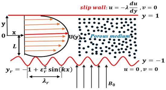
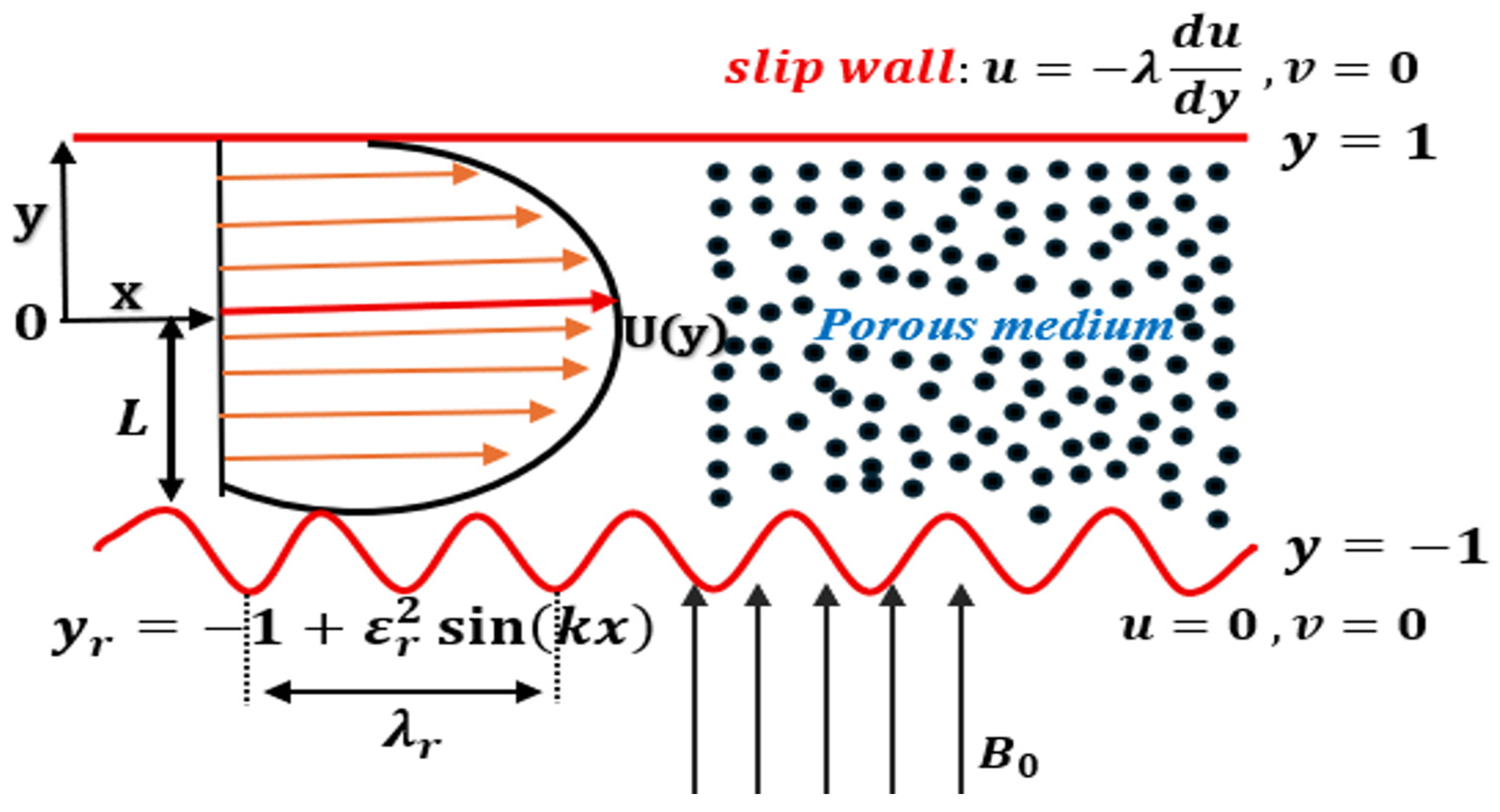
The present study investigates the linear stability of an incompressible magnetohydrodynamic (MHD) flow through a porous channel bounded by two parallel walls, as illustrated in Figure 1. The upper wall is smooth and satisfies the Navier-slip boundary condition. In contrast, the lower wall is periodically rough and satisfies the classical no-slip condition. To examine the influence of different wall boundary conditions on flow stability, two additional configurations are considered: Navier-slip conditions at both walls and no-slip conditions at both smooth walls.

Figure 1. Schematic of the physical model.

The fluid is assumed to be Newtonian, viscous, electrically conducting, and incompressible. It flows through a homogeneous porous medium under a uniform transverse magnetic field, $B=\left(0,B_0,0\right)$, imposed in the y-direction and perpendicular to the primary streamwise flow. The magnetic Reynolds number is assumed to be sufficiently small such that the induced magnetic field can be neglected. Consequently, the governing equations consist of the incompressible Navier–Stokes equations supplemented by Darcy drag and Lorentz-force terms to account for porous-medium resistance and magnetic effects. The resulting Lorentz force opposes the primary streamwise motion and therefore appears as an electromagnetic damping term in the streamwise momentum equation.

The smooth upper wall is located at $y=1$, whereas the lower wall is periodically corrugated and is represented by $y_r=-1+{\epsilon }_r^2\sin \left(kx\right)$, where ${\epsilon }_r\ll 1$ is the dimensionless roughness-amplitude parameter, and $k$ is the dimensionless roughness wavenumber. The corresponding dimensionless roughness wavelength is ${\lambda }_r={\displaystyle \frac{2\pi }{k}}.$ Thus, the wall displacement from its mean position is $\eta \left(x\right)={\epsilon }_r^2\sin \left(kx\right).$ Since ${\epsilon }_r\ll 1$, the boundary conditions imposed at the actual periodically modulated wall are expanded to first order in the wall displacement $\eta \left(x\right)$ about the mean wall position $y=-1$.

For a generic flow variable $f\left(x,y,t\right)$, the Taylor expansion about the mean lower-wall position gives

$$f\left(x,y_r,t\right)=f\left(x,-1,t\right)+\eta \left(x\right){\left.{\displaystyle \frac{\partial f}{\partial y}}\right|}_{y=-1}+O\left({\eta }^2\right).$$

Hence,

$$f\left(x,y_r,t\right)=f\left(x,-1,t\right)+{\epsilon }_r^2\sin \left(kx\right){\left.{\displaystyle \frac{\partial f}{\partial y}}\right|}_{y=-1}+O\left({\epsilon }_r^4\right).$$

At the actual corrugated lower wall $y=y_r$, the classical no-slip and impermeability conditions are imposed as $u\left(x,y_r,t\right)=0,v\left(x,y_r,t\right)=0$.

Using the above Taylor expansion, these conditions become

$$\begin{array}{c}u\left(x,-1,t\right)+{\epsilon }_r^2\sin \left(kx\right){\left.{\displaystyle \frac{\partial u}{\partial y}}\right|}_{y=-1}+O\left({\epsilon }_r^4\right)=0,\end{array}$$

and

$$\begin{array}{c}v\left(x,-1,t\right)+{\epsilon }_r^2\sin \left(kx\right){\left.{\displaystyle \frac{\partial v}{\partial y}}\right|}_{y=-1}+O\left({\epsilon }_r^4\right)=0.\end{array}$$

Figure 1 illustrates the physical configuration considered in the present study. The channel has a smooth upper wall at $y=1$ with Navier-slip condition and a periodically corrugated lower wall described by $\begin{array}{c}{y}_r=-1+{\epsilon }_r^2\sin \left(kx\right),\end{array}$ where $L$ denotes the channel half-width, $y=0$ is the channel centreline, ${\epsilon }_r$ is the dimensionless roughness amplitude, $k$ is the roughness wavenumber, and $\begin{array}{c}{\lambda }_r={\displaystyle \frac{2\pi }{k}}\end{array}$ is the corresponding roughness wavelength. The lower wall satisfies the classical no-slip condition, while $B_0$ represents the applied transverse magnetic field.

For an incompressible two-dimensional flow through a homogeneous porous medium, the dimensional continuity and momentum equations are given by [3,16,26]

$${\displaystyle \frac{\partial \tilde{u}}{\partial \tilde{x}}}+{\displaystyle \frac{\partial \tilde{v}}{\partial \tilde{y}}}=0$$

(4)

$${\displaystyle \frac{\partial \tilde{u}}{\partial \tilde{t}}}+\tilde{u}{\displaystyle \frac{\partial \tilde{u}}{\partial \tilde{x}}}+\tilde{v}{\displaystyle \frac{\partial \tilde{u}}{\partial \tilde{y}}}=-{\displaystyle \frac{1}{{\rho }_0}}{\displaystyle \frac{\partial \tilde{p}}{\partial \tilde{x}}}+\nu {\nabla }^2\tilde{u}-{\displaystyle \frac{\nu }{K}}\tilde{u}-{\displaystyle \frac{\sigma B_0^2}{{\rho }_0}}\tilde{u}$$

(5)

$${\displaystyle \frac{\partial \tilde{v}}{\partial \tilde{t}}}+\tilde{u}{\displaystyle \frac{\partial \tilde{v}}{\partial \tilde{x}}}+\tilde{v}{\displaystyle \frac{\partial \tilde{v}}{\partial \tilde{y}}}=-{\displaystyle \frac{1}{{\rho }_0}}{\displaystyle \frac{\partial \tilde{p}}{\partial \tilde{y}}}+\nu {\nabla }^2\tilde{v}-{\displaystyle \frac{\nu }{K}}\tilde{v}$$

(6)

where $\tilde{\mathbf{u}}=\left(\tilde{u},\tilde{v}\right)$ is the dimensional velocity vector, $\tilde{u}$ and $\tilde{v}$ are the streamwise and wall-normal velocity components, respectively. ${\rho }_0$ is the fluid density, $\nu$ is the kinematic viscosity, $p$ is the pressure, $\sigma$ is the electrical conductivity, $B_0$ is the strength of the applied uniform transverse magnetic field, and $K$ is the permeability of the porous medium.

Introducing the following dimensionless variables:

$$x={\displaystyle \frac{\tilde{x}}{L}},\hspace{1em}y={\displaystyle \frac{\tilde{y}}{L}}, u={\displaystyle \frac{\tilde{u}}{U_0}},\hspace{1em}v={\displaystyle \frac{\tilde{v}}{U_0}}, t={\displaystyle \frac{U_0}{L}}\tilde{t}, p={\displaystyle \frac{\tilde{p}-\widetilde{p_0}}{{\rho }_0{U}_0^2}}$$

(7)

where $L$ is the channel half-width and $U_0$ is the characteristic velocity.

Substituting the dimensionless variables defined in Equation (7) into Equations (4)–(6), we obtain the following dimensionless governing equations:

$${\displaystyle \frac{\partial u}{\partial x}}+{\displaystyle \frac{\partial v}{\partial y}}=0$$

(8)

$${\displaystyle \frac{\partial u}{\partial t}}+u{\displaystyle \frac{\partial u}{\partial x}}+v{\displaystyle \frac{\partial u}{\partial y}}=-{\displaystyle \frac{\partial p}{\partial x}}+{\displaystyle \frac{1}{Re}}{\nabla }^{2}u-\left({\displaystyle \frac{1}{Re Da}}+{\displaystyle \frac{{Ha}^2}{Re}}\right)u$$

(9)

$${\displaystyle \frac{\partial v}{\partial t}}+u{\displaystyle \frac{\partial v}{\partial x}}+v{\displaystyle \frac{\partial v}{\partial y}}=-{\displaystyle \frac{\partial p}{\partial y}}+{\displaystyle \frac{1}{Re}}{\nabla }^{2}v-{\displaystyle \frac{1}{Re Da}}v$$

(10)

where $\mathit{u}=\left(u,v\right)$ is the dimensionless velocity vector, $\mathrm{a}\mathrm{n}\mathrm{d} u$ and $v$ are the streamwise and wall-normal velocity components, respectively.

$$Re={\displaystyle \frac{U_{0}L}{\mathsf{\nu }}}, Da={\displaystyle \frac{K}{L^2}}, { Ha}^2={\displaystyle \frac{\mathsf{\sigma }{B}_0^2{L}^2}{\mathsf{\rho }\mathsf{\nu }}}$$

where $Re$, $Da$, and $Ha$ denote the Reynolds, Darcy, and Hartmann numbers, respectively.

Here, $L$ is the channel half-width, and $U_0$ is the fixed reference velocity used for non-dimensionalisation. The flow is driven by a prescribed constant pressure gradient, represented by the dimensionless parameter G. Accordingly, the Reynolds number is held fixed in the stability calculations, while variations in $Da,Ha$, and the slip parameter modify the resulting base-flow profile and its centreline velocity.

The Darcy number is defined as $Da=K/L^2$, where $K$ is the permeability of the porous medium. The present formulation is based on a homogenised porous-medium description and assumes that the small-amplitude periodic wall modulation does not alter the effective permeability of the porous medium. Accordingly, cases involving large values of $Da$ are interpreted as mathematical parameter-limit results, rather than as quantitative predictions for a specific porous material.

The linear stability analysis is performed for the three boundary configurations introduced in Section 2 to examine the combined effects of wall slip and surface roughness. Surface roughness is incorporated through a first-order perturbation correction to the governing equations and boundary conditions, providing a consistent representation of periodically rough surfaces while retaining the essential physics of disturbance growth and flow stability.

3. Linear Stability Analysis

The linear stability analysis is performed by considering two-dimensional infinitesimal disturbances. The flow variables are decomposed into a steady base flow, an infinitesimal hydrodynamic disturbance, and a roughness-induced correction.

Accordingly, the velocity and pressure fields are expressed as [16]

$$u\left(x,y,t\right)=U\left(y\right)+{\epsilon }_d\hspace{0.17em}{u}^{\ast }\left(x,y,t\right)+{{\epsilon }_r}^2{u}_b\left(x,y\right),$$

(11)

$$v\left(x,y,t\right)={\epsilon }_d\hspace{0.17em}{v}^{\ast }\left(x,y,t\right)+{{\epsilon }_r}^2{v}_b\left(x,y\right),$$

(12)

$$p\left(x,y,t\right)=P\left(x\right)+{\epsilon }_d\hspace{0.17em}{p}^{\ast }\left(x,y\right)+{{\epsilon }_r}^2{p}_b\left(x,y\right)$$

(13)

where $U\left(y\right)$ and $P\left(x\right)$ denote the steady base velocity and pressure, respectively. The quantities $u^{\ast }$, $v^{\ast }$, and $p^{\ast }$ denote the infinitesimal hydrodynamic disturbance fields, whereas $u_b$, $v_b$, and $p_b$ represent the flow corrections induced by the periodically corrugated lower wall. Since the wall displacement is $\eta \left(x\right)={\epsilon }_r^2\sin \left(kx\right)$, the corresponding roughness-induced corrections enter at $O\left({\epsilon }_r^2\right)$. Thus, ${\epsilon }_d$ and ${\epsilon }_r$ are distinct small parameters associated with the hydrodynamic disturbance and wall corrugation, respectively.

Substituting Equations (11)–(13) into Equations (8)–(10) yields the governing base-flow equations:

$${\displaystyle \frac{\partial U}{\partial x}}=0 \hspace{1em}\Rightarrow \hspace{1em}U=U(y),$$

(14)

$$-{\displaystyle \frac{dP}{dx}}+{\displaystyle \frac{1}{Re}}{\displaystyle \frac{d^{2}U}{d{y}^2}}-{\displaystyle \frac{1}{Re\hspace{0.17em}Da}}U-{\displaystyle \frac{H{a}^2}{Re}}U=0,$$

(15)

$${\displaystyle \frac{\partial P}{\partial y}}=0$$

(16)

Collecting the terms of $O\left({\epsilon }_d\right)$, the linearised perturbation equations are given by

$${\displaystyle \frac{\partial u^{\ast }}{\partial x}}+{\displaystyle \frac{\partial v^{\ast }}{\partial y}}=0$$

(17)

$${\displaystyle \frac{\partial u^{\ast }}{\partial t}}+\mathrm{U}{\displaystyle \frac{\partial u^{\ast }}{\partial x}}+v^{\ast }{\displaystyle \frac{dU}{dy}}=-{\displaystyle \frac{\partial p^{\ast }}{\partial x}}+{\displaystyle \frac{1}{Re}} {\nabla }^2{u}^{\ast }-\left({\displaystyle \frac{1}{Re Da}}+{\displaystyle \frac{{Ha}^2}{\mathrm{R}\mathrm{e}}}\right)u^{\ast }$$

(18)

$${\displaystyle \frac{\partial v^{\ast }}{\partial t}}+U{\displaystyle \frac{\partial v^{\ast }}{\partial x}}=-{\displaystyle \frac{\partial p^{\ast }}{\partial y}}+{\displaystyle \frac{1}{Re}}{\nabla }^2{v}^{\ast }-{\displaystyle \frac{1}{Re Da}}{v}^{\ast }$$

(19)

Since the present analysis is restricted to linear temporal stability, the disturbance expansion is truncated at first order in the independent disturbance-amplitude parameter ${\epsilon }_d$. The parameter ${\epsilon }_r\ll 1$ denotes the roughness-amplitude parameter, with the wall displacement specified at $O\left({{\epsilon }_r}^2\right)$. The effect of the periodically modulated lower wall is introduced through the boundary conditions imposed at $y_r=-1+{\epsilon }_r^2\mathrm{s}\mathrm{i}\mathrm{n}\left(kx\right)$, rather than through additional bulk equations. Expanding these conditions about the mean wall position $y=-1$ generates the roughness-dependent Fourier sidebands $\alpha +k$ and $\alpha -k$. In the present reduced single-sideband formulation, the $\left(\alpha +k\right)$ component is retained through the combined streamwise wavenumber $\alpha +k$, whereas the $\left(\alpha -k\right)$ component and the explicit $O\left({\epsilon }_r^2\right)$ boundary corrections are omitted as part of the adopted modelling approximation.

To satisfy the continuity equation, the disturbance velocity field is represented in terms of a stream-function. The stream-function is then expressed in normal-mode form as

$$\mathsf{\psi }\left(x,y,t\right)=\mathsf{\varphi }\left(x,y\right)e^{i\mathsf{\alpha }\left(x-ct\right)}$$

(20)

where $\varphi \left(x, y\right)$ is the disturbance stream-function amplitude, $\alpha \in \mathbb{R}$ is the disturbance wavenumber, and $c=c_r+i{c}_i\in \mathbb{C}$ is the complex wave speed.

The lower wall is assumed to have small-amplitude sinusoidal roughness. For $k>0$, the corresponding roughness wavelength is ${\lambda }_r={\displaystyle \frac{2\pi }{k}}$. The limiting case $k=0$ corresponds to the smooth-wall limit, for which $\sin \left(kx\right)=0$ and hence $y_r=-1$. The roughness-induced spatial dependence is represented as

$$\varphi \left(x,y\right)=\phi \left(y\right)\hspace{0.17em}{e}^{ikx}$$

(21)

where $k$ denotes the roughness wavenumber and $\phi \left(y\right)$ is the associated wall-normal amplitude function.

Combining the normal-mode representation with the spatial dependence introduced by the periodic wall roughness gives

$$\psi \left(x,y,t\right)=\phi \left(y\right)\hspace{0.17em}{e}^{i\left[\left(k+\alpha \right)x-\alpha ct\right]}$$

(22)

Thus, the periodic wall roughness enters the disturbance formulation through the combined streamwise wavenumber $\left(k+\alpha \right)$.

The periodic modulation of the lower wall introduces additional streamwise Fourier components into the disturbance field. The roughness-dependent part of the Taylor-expanded boundary condition contains the product $\mathrm{s}\mathrm{i}\mathrm{n}\left(kx\right)e^{i\alpha x}$, which can be written as

$$\mathrm{s}\mathrm{i}\mathrm{n}\left(kx\right)e^{i\alpha x}={\displaystyle \frac{1}{2i}}\left[e^{i\left(\alpha +k\right)x}-e^{i\left(\alpha -k\right)x}\right].$$

Thus, the first-order wall-displacement correction couples the primary disturbance of wavenumber $\alpha$ to the two sidebands $\alpha +k$ and $\alpha -k$. In the present reduced single-sideband approximation, the $+$ sideband $\left(\alpha +k\right)$ is retained, while the $-$ sideband $\left(\alpha -k\right)$ is omitted. Accordingly, the retained disturbance is represented as

$$\psi \left(x,y,t\right)=\varphi \left(y\right)e^{i\left[\left(\alpha +k\right)x-\alpha ct\right]},$$

The differential operators in the reduced Orr–Sommerfeld problem are evaluated using the combined streamwise wavenumber $\alpha +k.$ The explicit $O\left({\epsilon }_r^2\right)$ coefficient arising from the Taylor expansion is not retained as an independent boundary parameter in this reduced model; its spatial effect is represented through the selected $+$ sideband. Hence, the formulation should be interpreted as a reduced single-sideband model of the periodically modulated wall, rather than a full Floquet–Bloch treatment of the boundary-value problem [16].

The roughness amplitude ${\epsilon }_r$ is assumed to be sufficiently small such that the bulk porous-medium properties, including the prescribed permeability $K$, remain unchanged. Thus, the wall corrugation is treated as a small-amplitude geometric perturbation of the lower boundary, while its spatial variation is characterised by the roughness wavenumber $k$.

The disturbance velocity vector is defined as

$${ u}^{\ast }\left(x,y,t\right)={\displaystyle \frac{\partial \mathsf{\psi }}{\partial y}}={\phi }^{\prime }\left(y\right)e^{i\left[\right(k+\mathsf{\alpha })x-\mathsf{\alpha }ct]}$$

(23)

$$v^{\ast }\left(x,y,t\right)=-{\displaystyle \frac{\partial \mathsf{\psi }}{\partial x}}=-i(k+\mathsf{\alpha })\phi \left(y\right)e^{i\left[\right(k+\mathsf{\alpha })x-\mathsf{\alpha }ct]}$$

(24)

The above expressions satisfy the continuity equation identically.

Substituting Equations (23) and (24) into the perturbation Equations (17)–(19), and simplifying, we get

$$\begin{gathered} i(k+\alpha )p=i\left((k+\alpha )U-\alpha c\right)\phi -({\displaystyle \frac{1}{Re\hspace{0.17em}Da}}+{\displaystyle \frac{H{a}^2}{Re}}) D\phi +{\displaystyle \frac{1}{Re}}\left(D^3-{(k+\alpha )}^{2}D\right)\phi \\ +i(k+\alpha )U^{\prime }\phi \end{gathered}$$

(25)

$$p^{\prime }=(k+\alpha )\alpha c\hspace{0.17em}\phi +i{(k+\alpha )}^{2}U\hspace{0.17em}-{\displaystyle \frac{i(k+\alpha )}{Re}}\left(D^2-{(k+\alpha )}^2\right)\phi +{\displaystyle \frac{i(k+\alpha )}{Re\hspace{0.17em}Da}}\phi$$

(26)

Equations (20) and (21) incorporate the effect of periodic wall roughness through the combined streamwise wavenumber $(k+\alpha )$.

Eliminating the pressure terms from Equations (25) and (26) yields the following fourth-order modified Orr–Sommerfeld equation [29]:

$$\begin{gathered} c\alpha \left[{\left(k+\alpha \right)}^2-D^2\right]\phi =\{\left({\displaystyle \frac{1}{i\hspace{0.17em}Re}}\right){\left[D^2-{\left(k+\alpha \right)}^2\right]}^2+{\left(k+\alpha \right)}^{3}U \\ -\left(k+\alpha \right)\left(U{D}^2-D^{2}U\right)-{\displaystyle \frac{1}{Re}}\left({\displaystyle \frac{1}{Da}}+H{a}^2\right)\left[{\left(k+\alpha \right)}^2-D^2\right]\} \phi \end{gathered}$$

(27)

where $D={\displaystyle \frac{d}{dy}}$ denotes differentiation with respect to the wall-normal coordinate $y$, $\alpha$ is the real disturbance wavenumber, $k$ is the roughness wavenumber, and $c$ denotes the complex wave speed.

Equation (27) represents the modified Orr–Sommerfeld eigenvalue problem for MHD flow in a porous channel with periodic wall roughness. The effective streamwise wavenumber in the present single-sideband formulation is $\left(k+\alpha \right)$.

The complex wave speed is expressed as

$$c=c_r+i{c}_i$$

(28)

where $c_r$ is the phase speed of the disturbance, and $c_i$ is the temporal growth rate.

The flow is unstable for $\left(c_i>0\right)$ and stable for $\left(c_i<0\right)$.

For a temporal stability analysis, the flow is classified as follows:

• Stable if $c_i<0$,
• Unstable if $c_i>0$,
• Neutral if $c_i=0$.

From the complete eigenvalue spectrum, the eigenvalue with the largest imaginary part is selected as the most unstable and physically relevant mode. This eigenvalue is subsequently used to determine stability characteristics and critical conditions.

The modified Orr–Sommerfeld eigenvalue problem is solved numerically using the Chebyshev spectral collocation method, which ensures spectral convergence and highly accurate solutions for hydrodynamic stability analysis. Differentiation matrices based on the Chebyshev polynomials are constructed using the Gauss–Lobatto collocation points, and the derivatives in the equations are evaluated through these matrices. The resulting discretised equation is formulated as a generalised eigenvalue problem and solved using MATLAB R2024b [30]. Using the calculated eigenvalues, the disturbance growth rates, phase velocities, and critical Reynolds numbers are determined. Possible spurious eigenvalues are identified through convergence tests, and only converged eigenvalues are retained for the stability analysis.

4. Boundary Conditions

4.1. Case I: Upper-Wall Slip with No-Slip Rough Lower Wall

In this configuration, the upper wall is smooth and satisfies the Navier-slip boundary condition, whereas the lower wall is modelled as a rough surface. The corresponding boundary conditions for Equations (8)–(10) are

$$u+\mathsf{\lambda }{\displaystyle \frac{\partial u}{\partial y}}=0,\hspace{1em}v=0, on y=1$$

(29)

$$u=0,\hspace{1em}v=0, on y=y_r$$

(30)

where ${\epsilon }_r$ is the roughness amplitude and $k$ is the roughness wavenumber, with $y_r=-1+{\epsilon }_r^{2}sin\left(kx\right)$.

Since ${\epsilon }_r\ll 1$, the lower-wall boundary conditions are expanded about the mean wall position $y=-1$. For a generic field $f\left(x,y,t\right)$, the Taylor expansion at the corrugated wall gives

$$\begin{array}{c}f\left(x,y_r,t\right)=f\left(x,-1,t\right)+{\epsilon }_r^2\sin \left(kx\right){\left.{\displaystyle \frac{\partial f}{\partial y}}\right|}_{y=-1}+O\left({\epsilon }_r^4\right).\end{array}$$

Therefore, the leading-order roughness contribution enters explicitly through the term ${\epsilon }_r^2\sin \left(kx\right)\partial f/\partial y$.

$$u+\mathsf{\lambda }{\displaystyle \frac{\partial u}{\partial y}}=0,\hspace{1em}v=0, on y=1$$

(31)

$$u+{\epsilon }_r^2\sin \left(kx\right){\displaystyle \frac{\partial u}{\partial y}}=0,\hspace{1em}v+{\epsilon }_r^2\sin \left(kx\right){\displaystyle \frac{\partial v}{\partial y}}=0\hspace{1em}\mathrm{on} y=-1,$$

(32)

In the absence of roughness, i.e., ${\epsilon }_r\to 0$, Equation (32) reduces to the classical no-slip conditions $u=v=0$ at $y=-1$.

Substituting these conditions into Equations (11)–(13), the corresponding base-flow boundary conditions become

$$U+\mathsf{\lambda }{\displaystyle \frac{dU}{dy}}=0, on\hspace{1em}y=1$$

(33)

$$U=0, on\hspace{1em}y=-1$$

(34)

For the mean base flow, the zeroth-order condition at the mean lower-wall location is $U\left(-1\right)=0$. The geometric correction associated with the corrugated wall is retained through the Taylor term ${\epsilon }_r^2\sin \left(kx\right){\left.{\displaystyle \frac{dU}{dy}}\right|}_{y=-1},$ while the base-flow profile is evaluated on the mean channel geometry.

The disturbance velocity and pressure fields are denoted by $u^{\ast }$, $v^{\ast }$ and $p^{\ast }$, respectively, to distinguish them from the corresponding total fields. The perturbation boundary conditions are given by

$$u^{\ast }+\mathsf{\lambda }{\displaystyle \frac{\partial u^{\ast }}{\partial y}}=0,\hspace{1em}{v}^{\ast }=0, on\hspace{1em}y=1$$

(35)

$$u^{\ast }+{\epsilon }_r^2\sin \left(kx\right){\displaystyle \frac{\partial u^{\ast }}{\partial y}}=0,\hspace{1em}{v}^{\ast }+{\epsilon }_r^2\sin \left(kx\right){\displaystyle \frac{\partial v^{\ast }}{\partial y}}=0, on\hspace{1em}y=-1$$

(36)

The terms proportional to ${\epsilon }_r^2$ explicitly represent the leading-order influence of the periodic lower-wall corrugation. In the smooth-wall limit ${\epsilon }_r\to 0$, Equation (36) reduce to the usual no-slip disturbance conditions.

As demonstrated in Section 3, multiplication of these $O\left({\epsilon }_r^2\right)$ terms by the primary Fourier disturbance generates the sidebands $\alpha +k$ and $\alpha -k$. The present reduced model retains the $\left(\alpha +k\right)$ sideband in the eigenvalue equation, while the explicit amplitude-dependent boundary correction is not retained as an independent boundary operator.

Using Equations (14)–(16) together with the boundary conditions in Equations (33) and (34), the corresponding base-flow velocity profile is obtained as

$$U\left(y\right)={\displaystyle \frac{G}{M^2}}\left[1-{\displaystyle \frac{\left(2sinh\left(M\right)+\lambda Mcosh\left(M\right)\right)cosh\left(My\right)-\lambda Msinh\left(M\right)sinh\left(My\right)}{sinh\left(2M\right)+\lambda Mcosh\left(2M\right)}}\right]$$

(37)

where $M^2={\displaystyle \frac{1}{Da}}+H{a}^2, G=-Re\hspace{0.17em}{\displaystyle \frac{dp}{dx}}$ denotes the dimensionless imposed pressure-gradient parameter.

The modified Orr–Sommerfeld equation is solved subject to the boundary conditions obtained from the disturbance conditions above, given by

$$D\phi +\lambda D^2\phi =0,\hspace{1em}\phi =0, on\hspace{1em}y=1$$

(38)

$$D\phi =0,\hspace{1em}\phi =0, on\hspace{1em}y=-1$$

(39)

Equation (39) represents the leading-order disturbance boundary condition imposed at the mean position of the lower wall, $y=-1$. As given in Section 3, the Taylor expansion of the periodically modulated wall boundary generates the first-order Fourier sidebands $\alpha +k$ and $\alpha -k$. In the present reduced single-sideband formulation, the $\left(\alpha +k\right)$ sideband is retained in the modified Orr–Sommerfeld eigenvalue problem, whereas the $\left(\alpha -k\right)$ sideband and higher spatial harmonics are omitted as part of the adopted modelling approximation. The explicit $O\left({\epsilon }_r^2\right)$ amplitude-dependent contribution arising from the wall-displacement expansion is likewise not incorporated as an independent boundary operator.

4.2. Case II: Slip at Both Walls with Rough Lower Surface

In this configuration, both channel walls satisfy the Navier-slip boundary condition, while the lower wall is periodically modulated. Following the procedure described in Case I, the boundary conditions are expanded about the mean lower-wall position:

$$y=-1,\mathrm{with} y_r=-1+{\epsilon }_r^2\sin \left(kx\right).$$

Accordingly, the leading-order boundary conditions at the mean wall positions are obtained as

$$u+{\lambda }_1{\displaystyle \frac{\partial u}{\partial y}}=0,\hspace{1em}v=0, on y=1$$

(40)

$$u-{\lambda }_2{\displaystyle \frac{\partial u}{\partial y}}=0,\hspace{1em}v=0, on y=-1$$

(41)

where ${\lambda }_1$ and ${\lambda }_2$ denote the slip parameters at the upper and lower walls, respectively. The Taylor expansion of the lower-wall condition about the mean position $y=-1$ generates the first-order Fourier sidebands $\alpha +k$ and $\alpha -k$. In the present reduced single-sideband formulation, only the $\left(\alpha +k\right)$ sideband is retained, while the $\left(\alpha -k\right)$ sideband is omitted as part of the adopted modelling approximation. The explicit $O\left({\epsilon }_r^2\right)$ wall-displacement correction is not retained as an independent boundary operator; instead, the selected roughness-induced spatial dependence is incorporated into the eigenvalue problem through the combined streamwise wavenumber $\alpha +k$.

The corresponding base-flow boundary conditions are therefore

$$U+{\lambda }_1{\displaystyle \frac{dU}{dy}}=0, on\hspace{1em}y=1$$

(42)

$$U-{\lambda }_2{\displaystyle \frac{dU}{dy}}=0, on\hspace{1em}y=-1$$

(43)

The associated perturbation boundary conditions become

$$u^{\ast }+{\lambda }_1{\displaystyle \frac{\partial u^{\ast }}{\partial y}}=0,\hspace{1em}{v}^{\ast }=0, on y=1$$

(44)

$$u^{\ast }-{\lambda }_2{\displaystyle \frac{\partial u^{\ast }}{\partial y}}=0,\hspace{1em}{v}^{\ast }=0, on y=-1$$

(45)

Using Equations (14)–(16) together with the boundary conditions in Equations (42) and (43), the corresponding base-flow solution is obtained as

$$U\left(y\right)={\displaystyle \frac{G}{M^2}}\left[1-{\displaystyle \frac{[ 2a+M\left({\lambda }_1+{\lambda }_2\right)cosh\left(M\right)]cosh\left(My\right)-Ma\left({\lambda }_1-{\lambda }_2\right)sinh\left(My\right)}{sinh\left(2M\right)+M\left({\lambda }_1+{\lambda }_2\right)cosh\left(2M\right)+M^2{\lambda }_1{\lambda }_2 sinh\left(2M\right)}}\right]$$

(46)

where $a=sinh\left(M\right)$.

The modified Orr–Sommerfeld equation is solved subject to

$$D\phi +{\lambda }_1{D}^2\phi =0,\hspace{1em}\phi =0, on\hspace{1em}y=1$$

(47)

$$D\phi -{\lambda }_2{D}^2\phi =0,\hspace{1em}\phi =0, on\hspace{1em}y=-1$$

(48)

Accordingly, although the boundary conditions in Equations (44), (45), (47) and (48) are expressed at the mean wall positions, the effect of the periodic wall modulation is incorporated in the reduced eigenvalue problem through the retained sideband wavenumber $\alpha +k$. Thus, Equations (47) and (48) define the leading-order mean-wall boundary operator, whereas the roughness-induced modification enters through $k$ in the modified Orr–Sommerfeld equation. The omitted $\left(\alpha -k\right)$ sideband represents a modelling reduction rather than a higher-order roughness contribution.

4.3. Case III: No-Slip at Both Walls with Rough Lower Surface

For the limiting case $\lambda =0$ in Equation (37) or ${\lambda }_1={\lambda }_2=0$ in Equation (46), the Navier-slip condition reduces to the classical no-slip condition. The classical no-slip boundary condition is recovered at both channel walls. Under these conditions, the governing base-flow solution reduces to the classical magnetohydrodynamic Poiseuille flow profile given by

$$U\left(y\right)={\displaystyle \frac{G}{M^2}}\left[1-{\displaystyle \frac{\cosh \left(My\right)}{\cosh \left(M\right)}}\right]$$

(49)

The corresponding no-slip boundary conditions are

$$u=0,\hspace{1em}v=0, on\hspace{1em}y=\pm 1$$

(50)

Furthermore, in the limiting case $Da\to \infty$ and $Ha\to 0$, we have $M\to 0$, and the above expression (39) reduces to

$$U\left(y\right)={\displaystyle \frac{G}{2}}\left(1-y^2\right)$$

(51)

which is the classical plane-Poiseuille velocity profile. This limiting result confirms the consistency of the present formulation.

The corresponding Orr–Sommerfeld eigenvalue problem is solved subject to the classical no-slip perturbation boundary conditions.

$$\phi =0,\hspace{1em}D\phi =0\hspace{1em}on y=\pm 1$$

(52)

5. Results and Discussion

The modified Orr–Sommerfeld eigenvalue problem is solved numerically to investigate the linear-stability characteristics of magnetohydrodynamic flow through a porous channel. The effects of the slip parameters, roughness wavenumber, Hartmann number, and Darcy number on the eigenvalue spectrum, critical Reynolds number, neutral stability curves, and base-flow characteristics are examined for the three boundary configurations defined in Section 2. The numerical methodology is first validated against benchmark solutions, after which the influence of the governing parameters is discussed in detail. During the parameter studies, $Re$ and $G$ are kept fixed, while $Da,Ha,k$, and $\lambda$ are varied individually. Consequently, these parameters modify the base-flow profile and centreline velocity without changing the prescribed reference velocity scale used in the definition of $Re$.

5.1. Case I: Upper-Wall Slip with No-Slip Rough Lower Wall

The stability characteristics of the flow with an upper Navier-slip wall and a rough no-slip lower wall are investigated for fixed values of $Re=\mathrm{10,000},G=2,N=120, \mathrm{a}\mathrm{n}\mathrm{d} \alpha =1.$

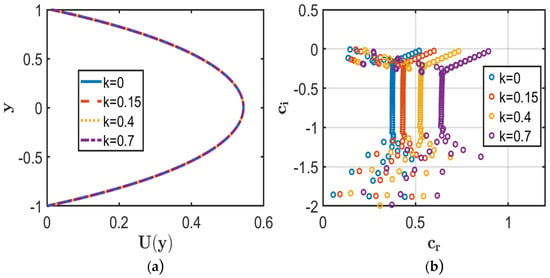
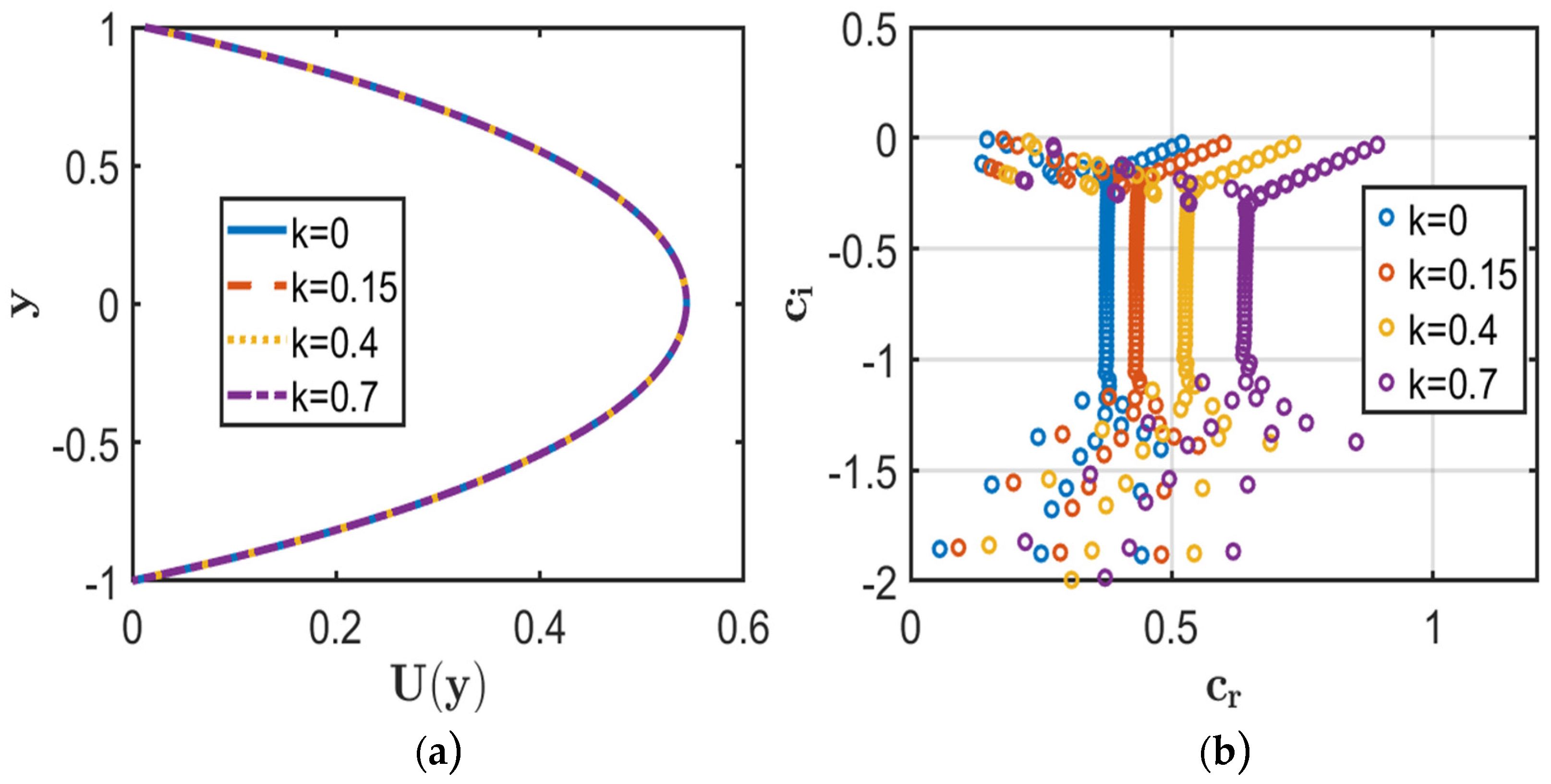
Figure 2 illustrates the influence of the roughness wavenumber $\left(k\right)$ on the base-flow velocity and eigenvalue spectrum. Figure 2a shows that varying $k$ has a negligible effect on the base-flow velocity profile, since $k$ characterises the spatial frequency of the wall roughness and does not enter the leading-order steady base-flow equation. Its influence is primarily evident in the roughness-dependent disturbance boundary conditions.

Figure 2. Effect of the roughness wavenumber (k = 0, 0.15, 0.4, 0.7) for fixed parameters Da = Ha = 1, and λ = 0.01. (a) Velocity profiles. (b) Eigenvalue spectrum.

The eigenvalue distributions in Figure 2b exhibit a progressive change with increasing $k$, with the dominant eigenvalues shifting toward lower values of $c_i$. Because $c_i<0$ corresponds to temporal decay and a stable disturbance, while $c_i>0$ indicates disturbance growth and instability, the observed decrease in $c_i$ indicates enhanced damping. Thus, within the investigated parameter range, increasing the roughness wavenumber tends to stabilise the flow while producing negligible changes in the base-flow velocity profile.

Table 2 quantitatively supports the spectral behaviour shown in Figure 2b. The imaginary part of the dominant eigenvalue, $c_i$, decreases as the roughness wavenumber $k$ increases, indicating a progressive reduction in the disturbance growth rate. The numerical results, therefore, confirm the stability trend observed in the eigenvalue spectra.

Table 2. Effect of roughness wavenumber (k) on the complex wave speed and stability characteristics.

k	c = cr + ici	Stability
0	0.14664 − 0.006973i	Stable
0.15	0.17777 − 0.007723i	Stable
0.4	0.22652 − 0.017333i	Stable
0.7	0.893018 − 0.030637i	Stable

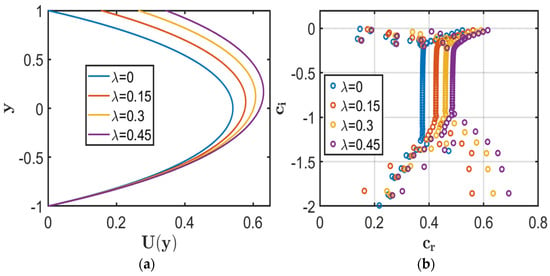
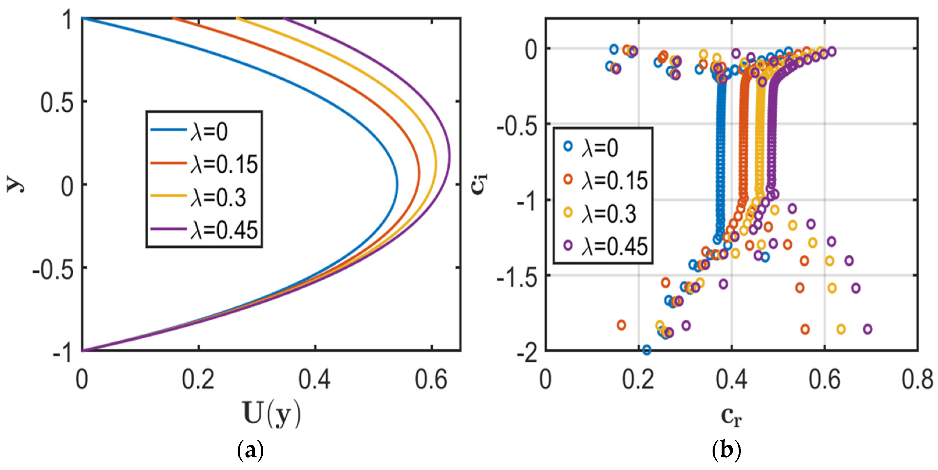
Figure 3 illustrates the influence of the slip parameter $\left(\lambda \right)$ on the base-flow velocity and eigenvalue spectrum. As seen in Figure 3a, increasing $\lambda$ enhances the streamwise velocity and shifts the maximum velocity toward the upper wall. This behaviour results from reduced wall shear and friction due to increased slip, thereby allowing greater fluid motion under the imposed pressure gradient.

Figure 3. Effect of the slip parameter λ = (0, 0.15, 0.3, 0.45) for fixed parameters Da = Ha = 1, and k = 0.01. (a) Velocity profiles. (b) Eigenvalue spectrum.

The eigenvalue spectrum in Figure 3b indicates that increasing $\lambda$ shifts the dominant eigenvalues toward larger $c_r$ and more negative $c_i$. Since $c_i<0$ corresponds to temporal decay, all considered cases remain stable. Thus, increasing wall slip enhances disturbance damping and maintains flow stability within the investigated parameter range.

Table 3 shows the most unstable eigenvalues. The imaginary part of the dominant eigenvalue, $c_i$, progressively decreases with increasing slip parameter, indicating stronger disturbance damping. Since $c_i <0$ for all cases, the flow remains stable throughout the investigated range.

Table 3. Effect of slip parameter on the complex wave speed and stability characteristics.

λ	c = cr + ici	Stability
0	0.14716 − 0.006496i	Stable
0.15	0.17499 − 0.011050i	Stable
0.3	0.18488 − 0.016234i	Stable
0.45	0.18929 − 0.019329i	Stable

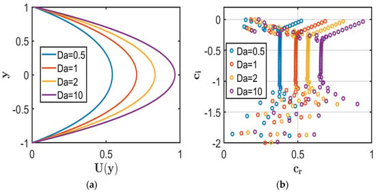
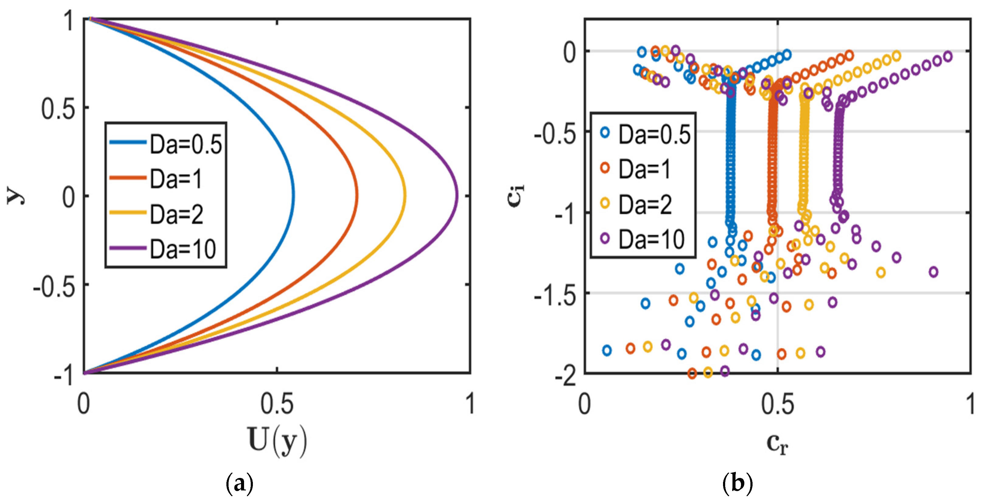
Figure 4 illustrates the effect of the Darcy number $\left(Da\right)$ on the base-flow velocity and eigenvalue spectrum. Figure 4a indicates that increasing $Da$ enhances the streamwise velocity throughout the channel, as higher permeability reduces the resistance offered by the porous medium and permits stronger pressure-driven flow.

Figure 4. Effect of the Darcy parameter Da = (0.5, 1, 2, 10) for fixed parameters Ha = 0.1, and λ = k = 0.01. (a) Velocity profiles. (b) Eigenvalue spectrum.

The eigenvalue distribution in Figure 4b shifts toward higher $c_r$ and $c_i$, with $c_i$ approaching zero from below. Since $c_i<0$ denotes temporal decay and stability, increasing $Da$ progressively weakens disturbance damping. When $c_i>0$, disturbances grow, and the flow becomes unstable. Thus, increasing $Da$ reduces the stabilising influence of the porous medium and promotes instability.

Table 4 shows the corresponding dominant eigenvalues for different Darcy numbers. The imaginary part of the dominant eigenvalue, $c_i,$ increases toward zero as $Da$ increases because the associated Darcy resistance decreases, thereby reducing the damping of hydrodynamic disturbances. This reduction in porous-medium damping eventually causes $c_i$ to become positive, marking the onset of instability.

Table 4. Effect of Darcy number Da on the complex wave speed and flow stability.

Da	c = cr + ici	Stability
0.5	0.14844 − 0.006942i	Stable
1	0.18324 − 0.002920i	Stable
2	0.20877 − 0.000397i	Stable
2.3	0.21271 − 0.000042i	Stable
2.35	0.21328 + 0.000008i	Unstable
10	0.23589 + 0.001848i	Unstable

It should be noted that $Da=2.35$ lies in the large-$Da$ regime. Since $Da=K/L^2$, such a value corresponds to a permeability scale comparable to or larger than the square of the channel half-width. Therefore, this result is interpreted as a mathematical stability characteristic of the present model rather than as a quantitatively representative prediction for a conventional homogenised porous medium.

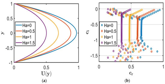
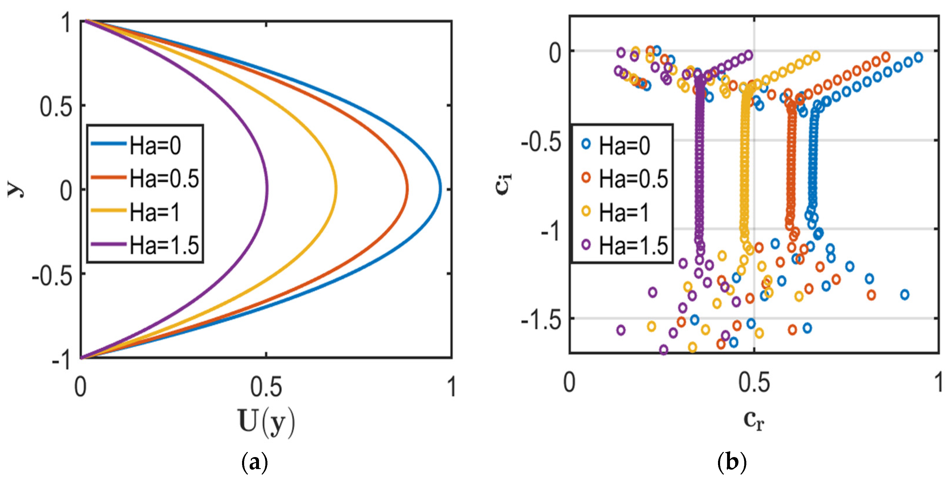
Figure 5 illustrates the influence of the Hartmann number $\left(Ha\right)$ on the base-flow velocity and eigenvalue spectrum. As observed in Figure 5a, increasing $Ha$ progressively reduces the streamwise velocity because the transverse magnetic field generates a Lorentz force opposing the fluid motion. Consequently, stronger magnetic effects increase electromagnetic resistance and suppress the base-flow velocity.

Figure 5. Effect of the Hartmann number Ha = (0, 0.5, 1, 1.5) for fixed parameters λ = k = 0.01, and Da = 10. (a) Velocity profiles. (b) Eigenvalue spectrum.

The results in Figure 5b indicate a systematic shift of the dominant eigenvalues toward lower $c_r$ and more negative $c_i$ as $Ha$ increases. The enhanced magnetic damping suppresses disturbance growth, with $c_i>0$ corresponding to an unstable flow and $c_i<0$ to a stable flow. Within the considered parameter range, the flow changes from unstable to stable as the magnetic field strength increases.

Table 5 further confirms this behaviour through the dominant eigenvalues, where $c_i$ decreases with increasing $Ha$. The sign change of $c_i$ identifies the transition from temporal disturbance growth to decay, demonstrating the stabilising influence of the transverse magnetic field.

Table 5. Effect of Hartmann number on the complex wave speed and flow stability.

Ha	c = cr + ici	Stability
0	0.23667 + 0.001905i	Unstable
0.5	0.21874 + 0.000481i	Unstable
0.55	0.21535 + 0.000190i	Unstable
0.6	0.21178 − 0.000125i	Stable
1	0.17936 − 0.003337i	Stable
1.5	0.13970 − 0.008040i	Stable

5.2. Case II: Slip at Both Walls with Rough Lower Surface

The stability characteristics of the flow with Navier-slip conditions at both walls and a rough lower surface are investigated for fixed values of $Re=\mathrm{10,000},\alpha =1,G=2,$ and $N=120$.

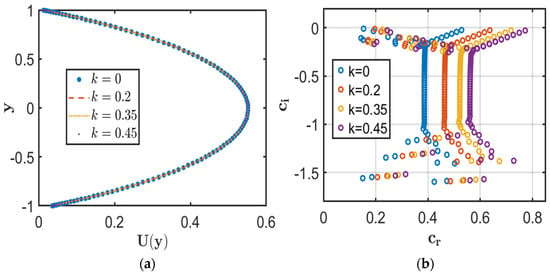
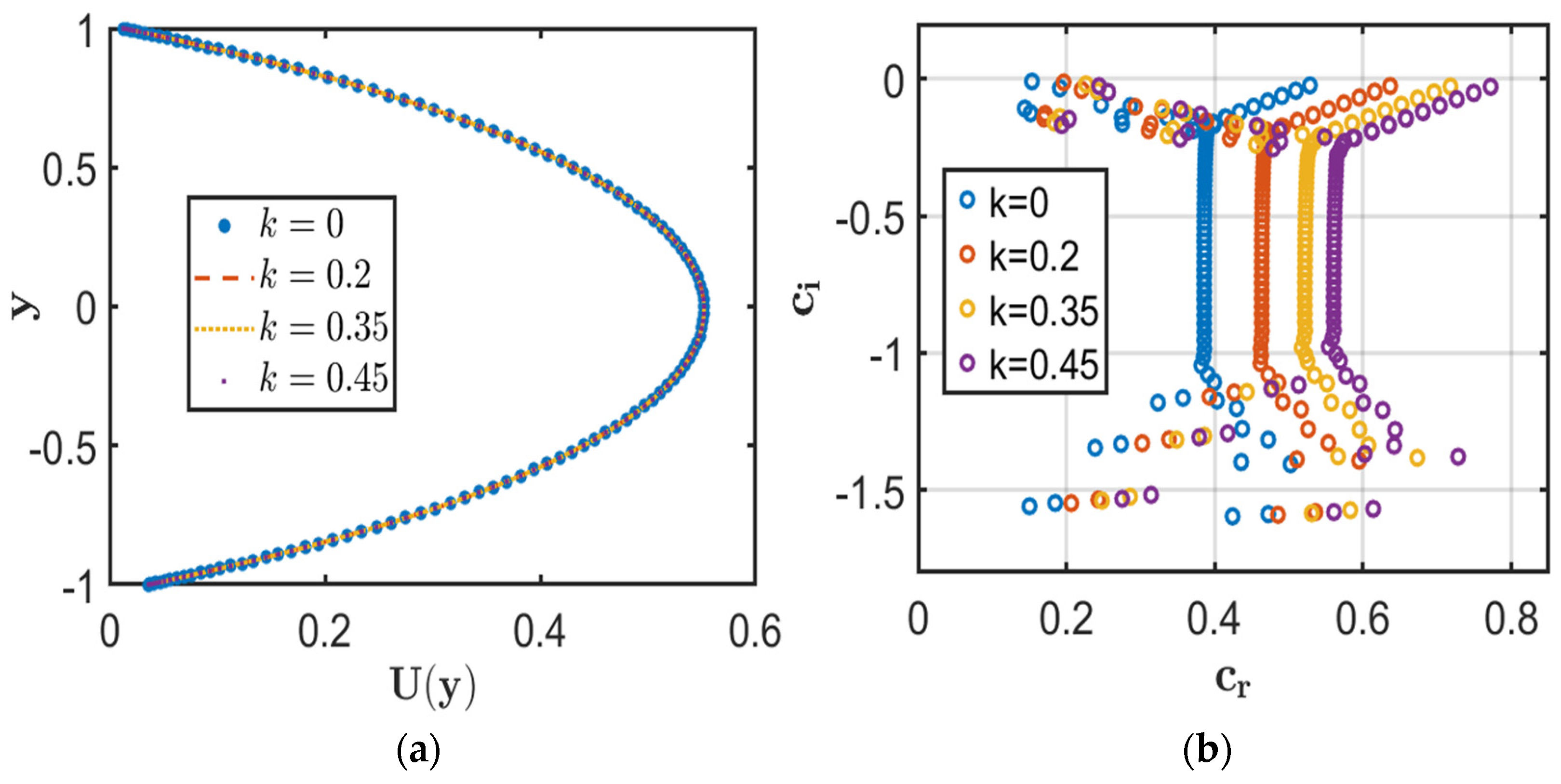
Figure 6 shows the effect of the roughness wavenumber $\left(k\right)$ on the base-flow velocity and eigenvalue spectrum for the configuration with Navier-slip at both walls. Figure 6a shows that the base-flow velocity profiles remain essentially unchanged as the roughness wavenumber $k$ increases. The imposed slip conditions modify the velocity distribution, whereas the roughness wavenumber has no significant effect on the leading-order base-flow velocity profile.

Figure 6. Effect of the roughness wavenumber k = (0, 0.2, 0.35, 0.45) for fixed parameters Da = Ha = 1, λ₁ = 0.01, and λ₂ = 0.03. (a) Velocity profiles. (b) Eigenvalue spectrum.

Figure 6b shows a systematic displacement of the dominant eigenvalues toward larger $c_r$ and more negative $c_i$ as $k$ increases. Within the considered parameter range, the reduction in $c_i$ indicates enhanced temporal damping of the disturbance modes, with all cases satisfying $c_i<0$, confirming that the flow remains stable.

Table 6 presents the corresponding dominant eigenvalues. The increasingly negative values of $c_i$ provide a quantitative measure of greater disturbance attenuation, while all computed modes remain stable.

Table 6. Effect of roughness wavenumber on the complex wave speed and flow stability.

k	c = cr + ici	Stability
0	0.15350 − 0.008813i	Stable
0.2	0.19625 − 0.012076i	Stable
0.35	0.22616 − 0.019365i	Stable
0.45	0.24406 − 0.026063i	Stable

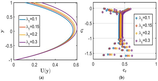
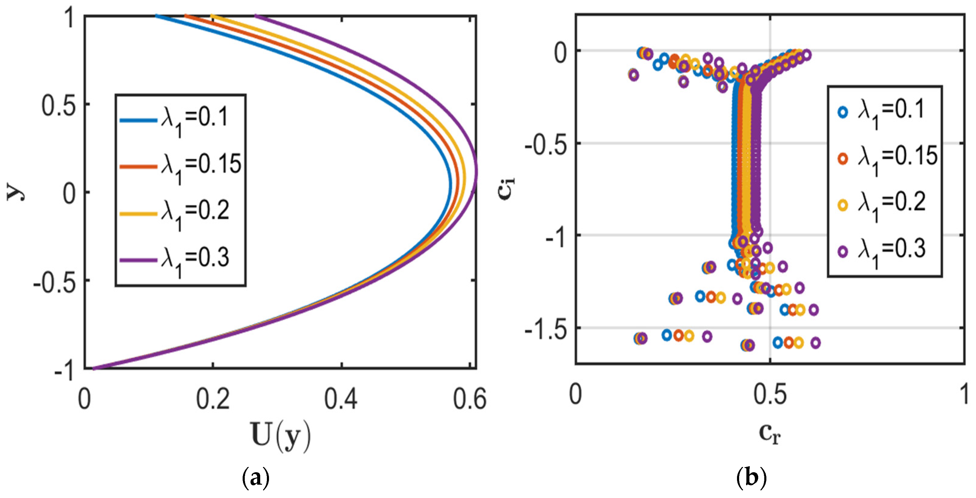
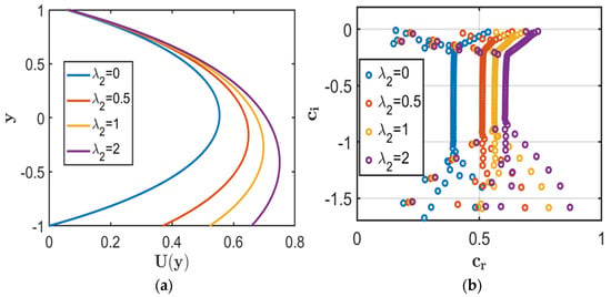
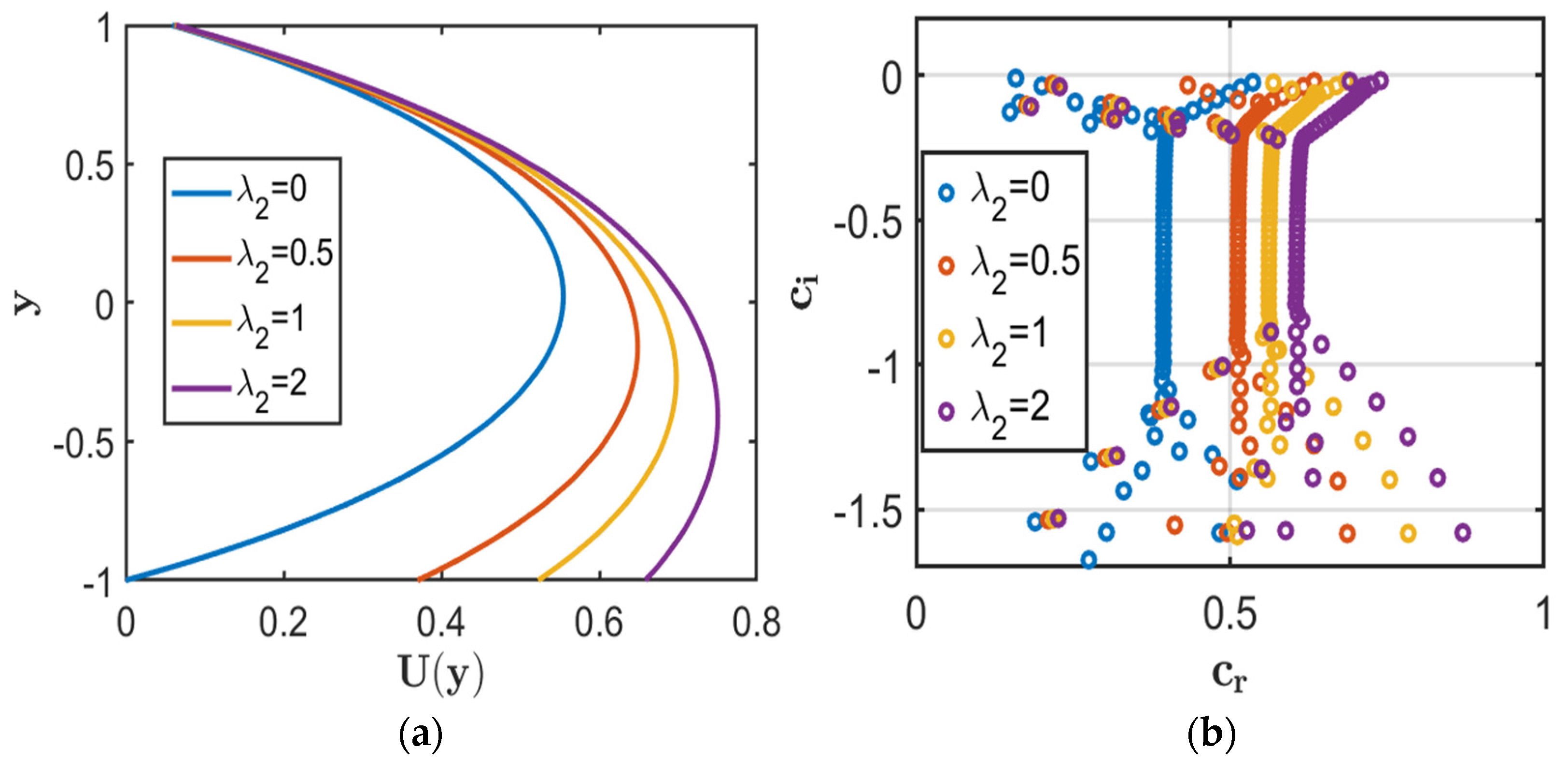
Figure 7 and Figure 8 illustrate the effects of the upper-wall slip parameter $\left({\lambda }_1\right)$ and lower-wall slip parameter $\left({\lambda }_2\right)$ on the base-flow velocity and eigenvalue spectrum for the configuration with slip at both walls and a rough lower surface. As observed in Figure 7a, increasing ${\lambda }_1$ enhances the streamwise velocity by reducing tangential resistance at the upper wall. The dominant eigenvalues in Figure 7b shift toward larger $c_r$ and more negative $c_i$, indicating enhanced temporal damping. Since $c_i<0$ corresponds to temporal decay, the flow remains stable for all considered values of ${\lambda }_1$.

Figure 7. Effect of the slip parameter λ₁ = (0.1, 0.15, 0.2, 0.3) for fixed parameters Da = Ha = 1, and λ₂ = k = 0.01. (a) Velocity profiles. (b) Eigenvalue spectrum.

Figure 8. Effect of the slip parameter λ₂ = (0, 0.5, 1, 2) for fixed parameters Da = Ha = 1, λ₁ = 0.05, and k = 0.01. (a) Velocity profiles. (b) Eigenvalue spectrum.

For the lower-wall slip parameter, Figure 8a shows that increasing ${\lambda }_2$ increases the streamwise velocity and modifies the asymmetric velocity distribution. This results from reduced tangential resistance at the lower wall. The eigenvalue spectrum in Figure 8b shifts toward larger $c_r$, while $c_i$ remains negative. Hence, all considered cases satisfy $c_i<0$, confirming that the flow remains stable over the investigated range of ${\lambda }_2$.

Table 7 lists the corresponding dominant eigenvalues for the two slip parameters. As ${\lambda }_1$ increases, $c_i$ decreases from $-0.010733 to -0.017563$, indicating enhanced disturbance attenuation. As ${\lambda }_2$ increases, $c_i$ remains negative throughout, confirming the stable nature of the flow for all considered cases.

Table 7. Effect of the slip parameters on the complex wave speed and flow stability.

λ1	λ2	c = cr + ici	Stability
0.1	0.01	0.17031 − 0.010733i	Stable
0.15	0.01	0.17715 − 0.012166i	Stable
0.2	0.01	0.18170 − 0.01421i	Stable
0.3	0.01	0.18699 − 0.017563i	Stable
0.05	0	0.15895 − 0.009040i	Stable
0.05	0.5	0.63409 − 0.020888i	Stable
0.05	1	0.68502 − 0.019366i	Stable
0.05	2	0.73973 − 0.017566i	Stable

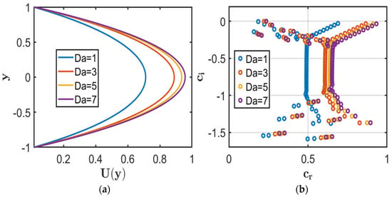
The effect of the Darcy number (Da) on the base-flow distribution and the eigenvalue spectra is illustrated in Figure 9 for MHD flow through a porous channel with slip at both boundaries. Figure 9a illustrates the effect of the Darcy number on the base-flow velocity. Increasing $Da$ progressively enhances the streamwise velocity, with the maximum velocity increasing as the porous-medium resistance decreases. This behaviour follows from the inverse dependence of the Darcy drag on $Da$, whereby larger $Da$ reduces the resistance to fluid motion and allows a stronger flow under the imposed pressure gradient.

Figure 9. Effect of the Darcy number Da = (1, 3, 5, 7) for fixed parameters Ha = 0.1, and λ₁ = λ₂ = k = 0.01. (a) Velocity profiles. (b) Eigenvalue spectrum.

Figure 9b shows a systematic modification of the eigenvalue spectrum as $Da$ increases. The dominant eigenvalues shift toward larger $c_r$, while $c_i$ increases toward zero and eventually becomes positive. This behaviour results from the reduced porous-medium resistance at larger $Da$, which weakens disturbance damping and ultimately drives the flow toward instability.

Table 8 quantifies the stability transition associated with $Da$. The dominant approaches zero as it increases and changes sign between $Da=3.8$ and $Da=3.9$. This sign reversal marks the critical condition at which disturbance decay changes to temporal growth, indicating the onset of flow instability.

Table 8. Effect of the Darcy parameter on the complex wave speed and flow stability.

Da	c = cr + ici	Stability
1	0.18556 − 0.003569i	Stable
3	0.22241 − 0.000387i	Stable
3.5	0.22569 − 0.000145i	Stable
3.8	0.22728 − 0.000030i	Stable
3.9	0.22777 + 0.000003i	Unstable
5	0.23188 + 0.000291i	Unstable
7	0.23622 + 0.000584i	Unstable

Similarly, the instability observed at $Da=3.9$ should be regarded as a limiting mathematical result of the model. The physical interpretation of such large Darcy numbers is restricted by the homogenised porous-medium assumption adopted in the present analysis.

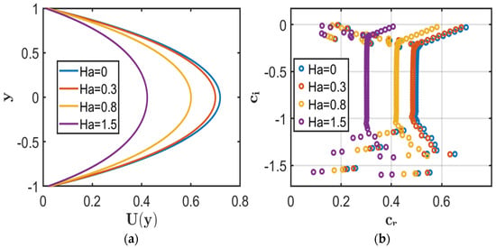
Figure 10 illustrates the effect of the Hartmann number ($Ha$) on the base-flow velocity and eigenvalue spectrum. Figure 10a shows the influence of the Hartmann number on the base-flow velocity. Increasing $Ha$ progressively suppresses the streamwise velocity, with the maximum velocity decreasing as the magnetic field strength increases. This reduction is caused by the Lorentz force, which acts as an electromagnetic drag opposing the fluid motion. Consequently, the enhanced magnetic resistance reduces the fluid momentum and lowers the base-flow velocity.

Figure 10. Effect of the Hartmann number Ha = (0, 0.3, 0.8, 1.5) for fixed parameters Da = 1, λ₂ = 0.02, and λ₁ = k = 0.01. (a) Velocity profiles. (b) Eigenvalue spectrum.

Figure 10b shows a systematic modification of the eigenvalue spectrum as $Ha$ increases. The dominant eigenvalues shift toward lower $c_r$ and more negative $c_i$ as the magnetic field strength increases. The decrease in $c_i$ reflects enhanced temporal damping of the disturbance modes due to the additional electromagnetic resistance introduced by the Lorentz force. Consequently, stronger magnetic damping suppresses disturbance growth and maintains flow stability over the considered parameter range.

Table 9 presents the corresponding dominant eigenvalues. The progressive decrease in $c_i$ with increasing $Ha$ indicates enhanced magnetic damping of the dominant disturbance mode. Since $c_i$ remains negative in all cases, the disturbances decay over time, and the flow remains stable.

Table 9. Effect of the Hartmann number on the complex wave speed and flow stability.

Ha	c = cr + ici	Stability
0	0.18963 − 0.004581i	Stable
0.3	0.18552 − 0.004938i	Stable
0.8	0.16412 − 0.006958i	Stable
1.5	0.124147 − 0.011332i	Stable

5.3. Case III: No-Slip at Both Walls with Lower-Wall Roughness

The stability characteristics of the flow with no-slip conditions at both walls and a periodically rough lower wall are investigated for fixed values of $Re=\mathrm{10,000}$, $N=120,$ $\alpha =1$, and $G=2$. The no-slip conditions impose maximum wall shear resistance, while the lower-wall roughness modifies the disturbance dynamics. The corresponding eigenvalue spectrum provides a reference for assessing the combined influence of surface roughness and wall boundary conditions on flow stability.

Figure 11 shows the base-flow velocity profile for classical MHD Poiseuille flow with no-slip boundary conditions at both walls. The velocity vanishes at the walls and reaches its maximum at the channel centerline, reflecting the balance between the imposed pressure gradient and viscous forces.

Figure 11. Velocity profile for the no-slip case with fixed values Da = Ha = 1, and k = 0.1.

Figure 12 compares the corresponding eigenvalue spectra for smooth- and rough-wall configurations. As shown in Figure 12a, several eigenvalues lie in the unstable region $\left(c_i>0\right),$ indicating disturbance growth. In contrast, the inclusion of wall roughness in Figure 12b shifts the eigenvalues toward the stable region $\left(c_i<0\right)$, demonstrating a stabilising effect within the considered parameter range. This result indicates that introducing wall roughness modifies the disturbance characteristics and suppresses the growth of unstable modes under the present no-slip boundary conditions.

Figure 12. Eigenvalue spectrum for fixed parameters Da = Ha = 1. (a) Eigenvalue spectrum for no-slip with no surface roughness (λ₁ = λ₂ = k = 0). (b) Eigenvalue spectrum for no-slip (λ₁ = λ₂ = 0) with roughness (k = 0.1).

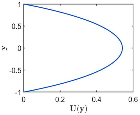
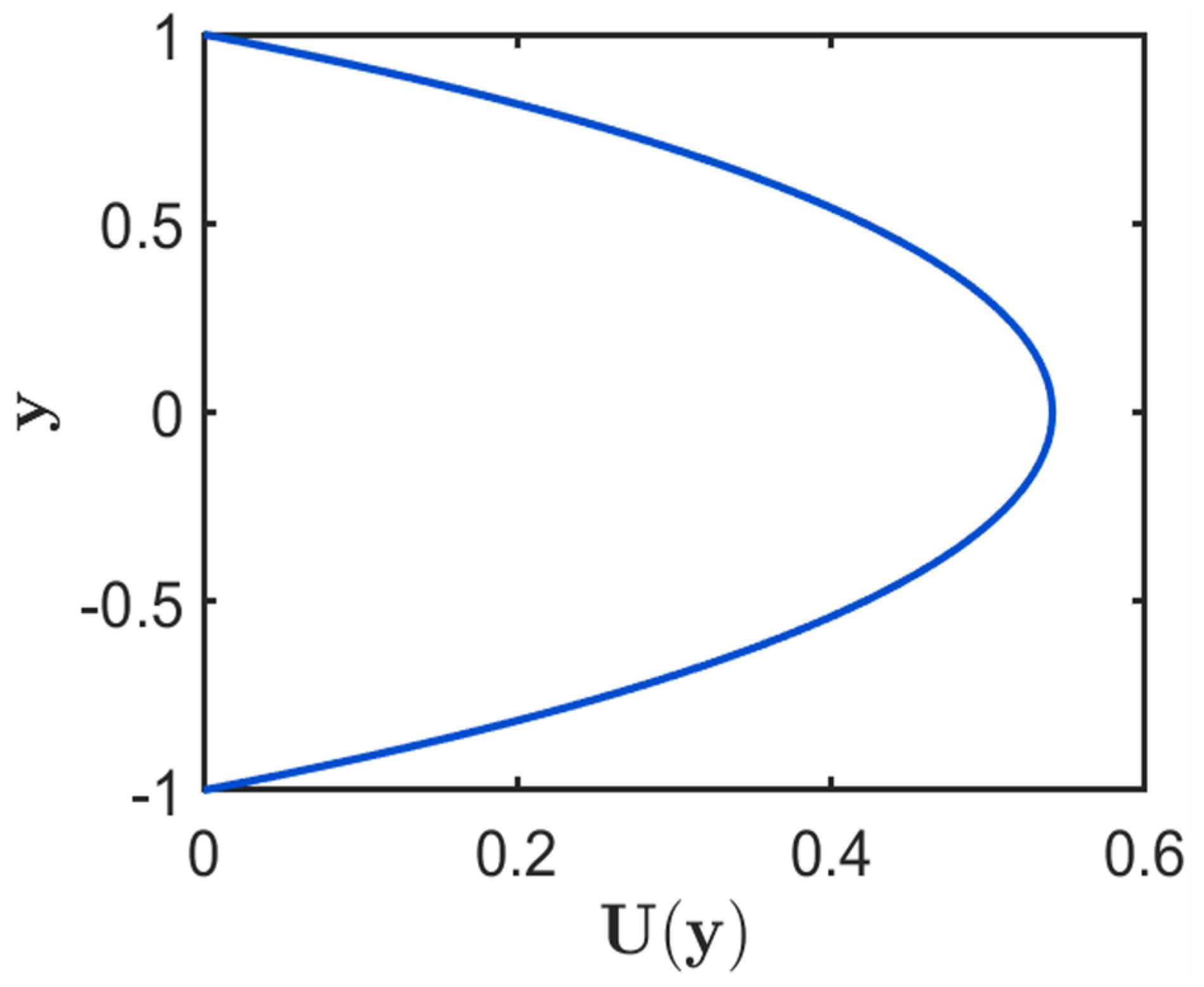
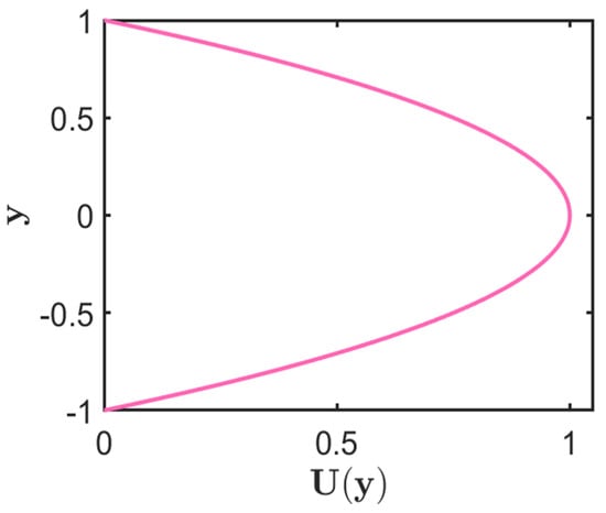
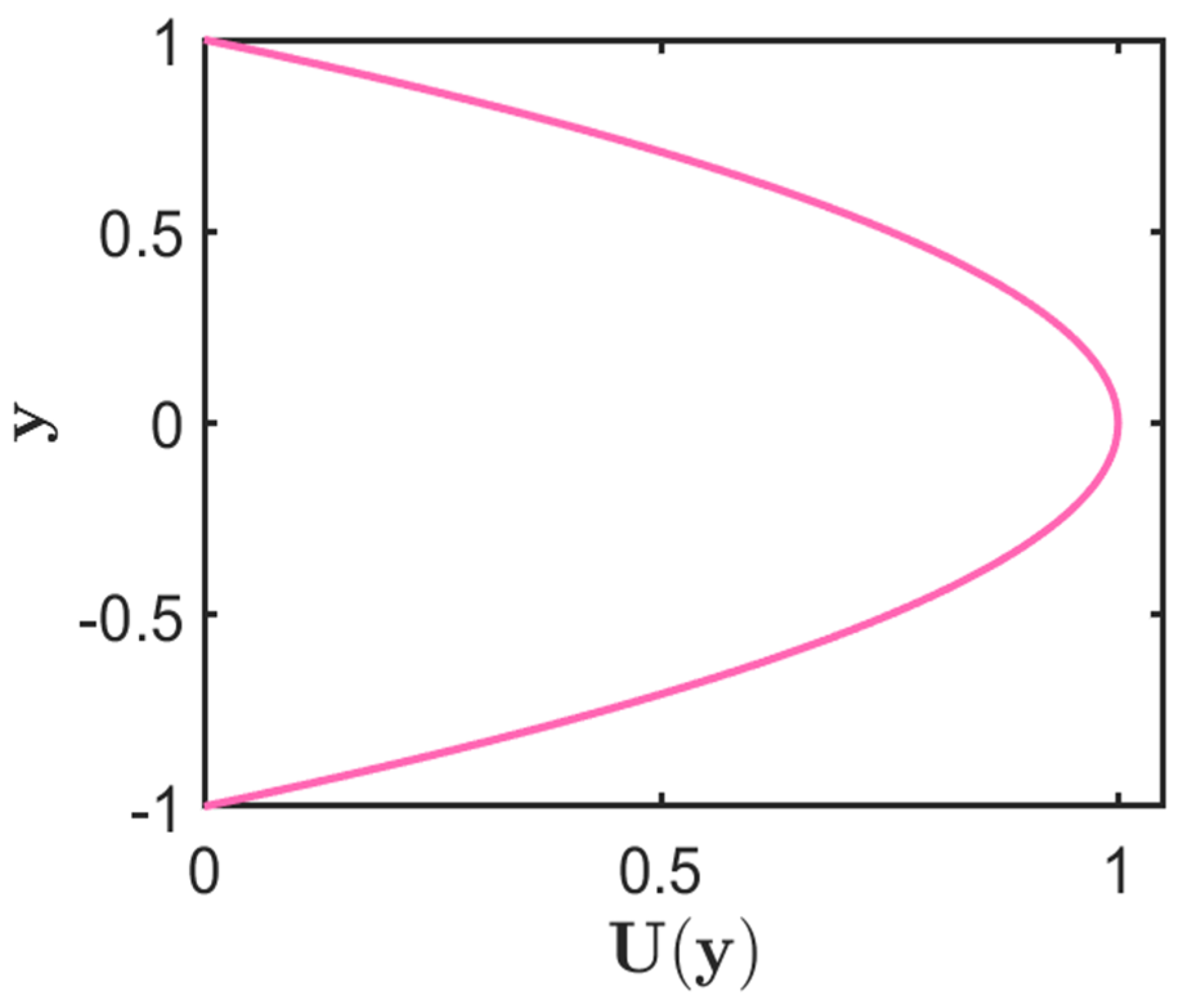
Figure 13 shows the classical parabolic base-flow velocity profile for plane Poiseuille flow without magnetic-field and porous-medium effects. The velocity reaches its maximum at the channel centreline. It decreases to zero at both walls because of the no-slip boundary condition.

Figure 13. Velocity profile for plane Poiseuille flow in the limiting case $Da\to \infty$ and Ha = 0.

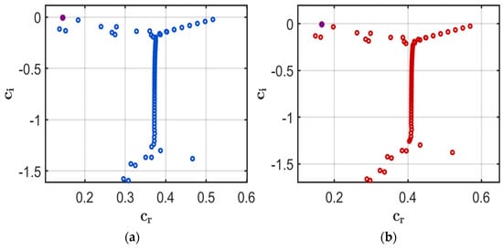
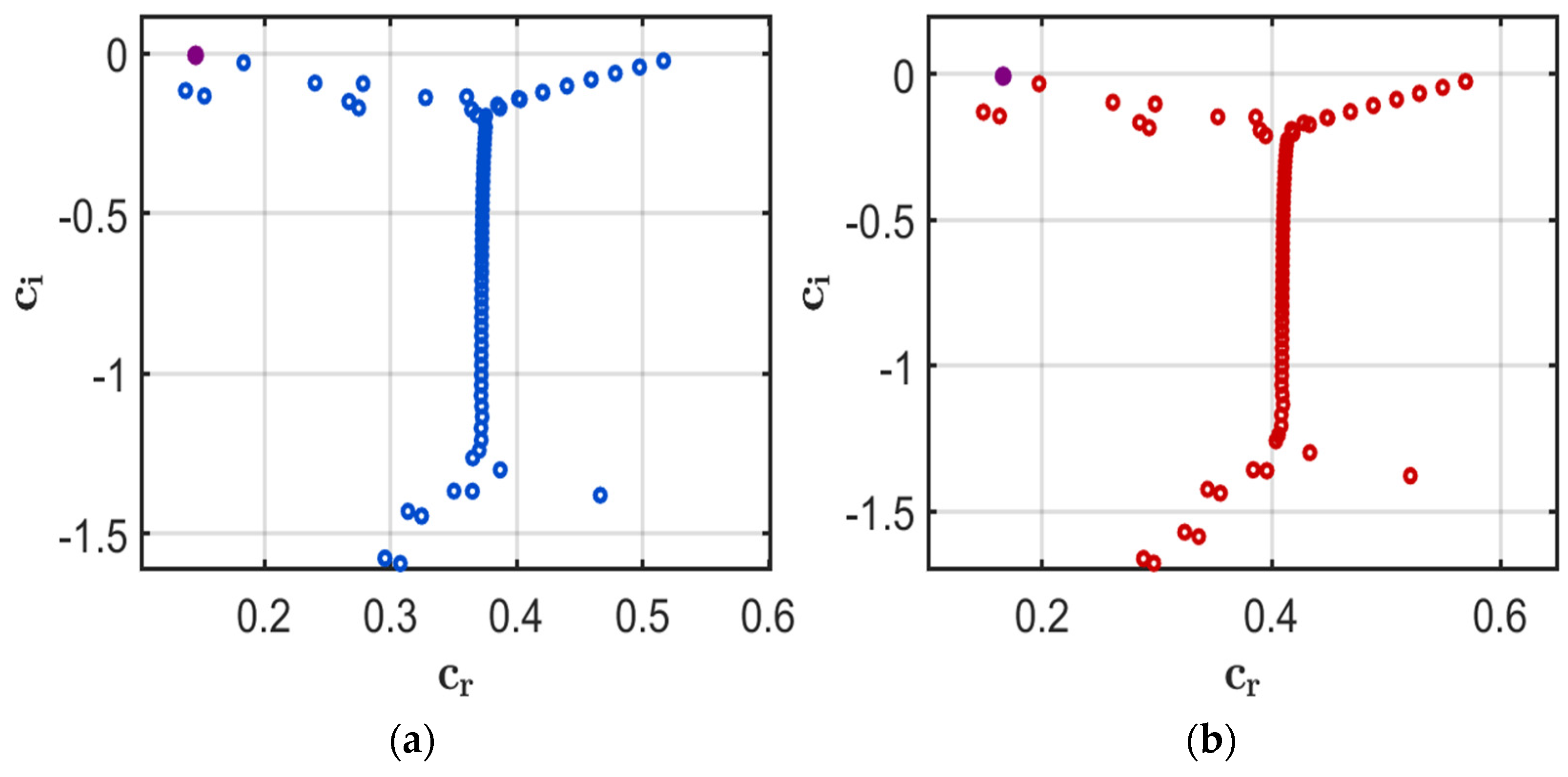
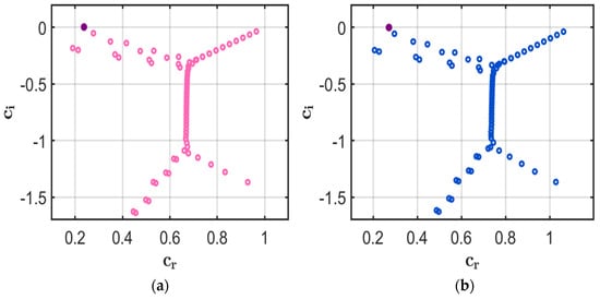
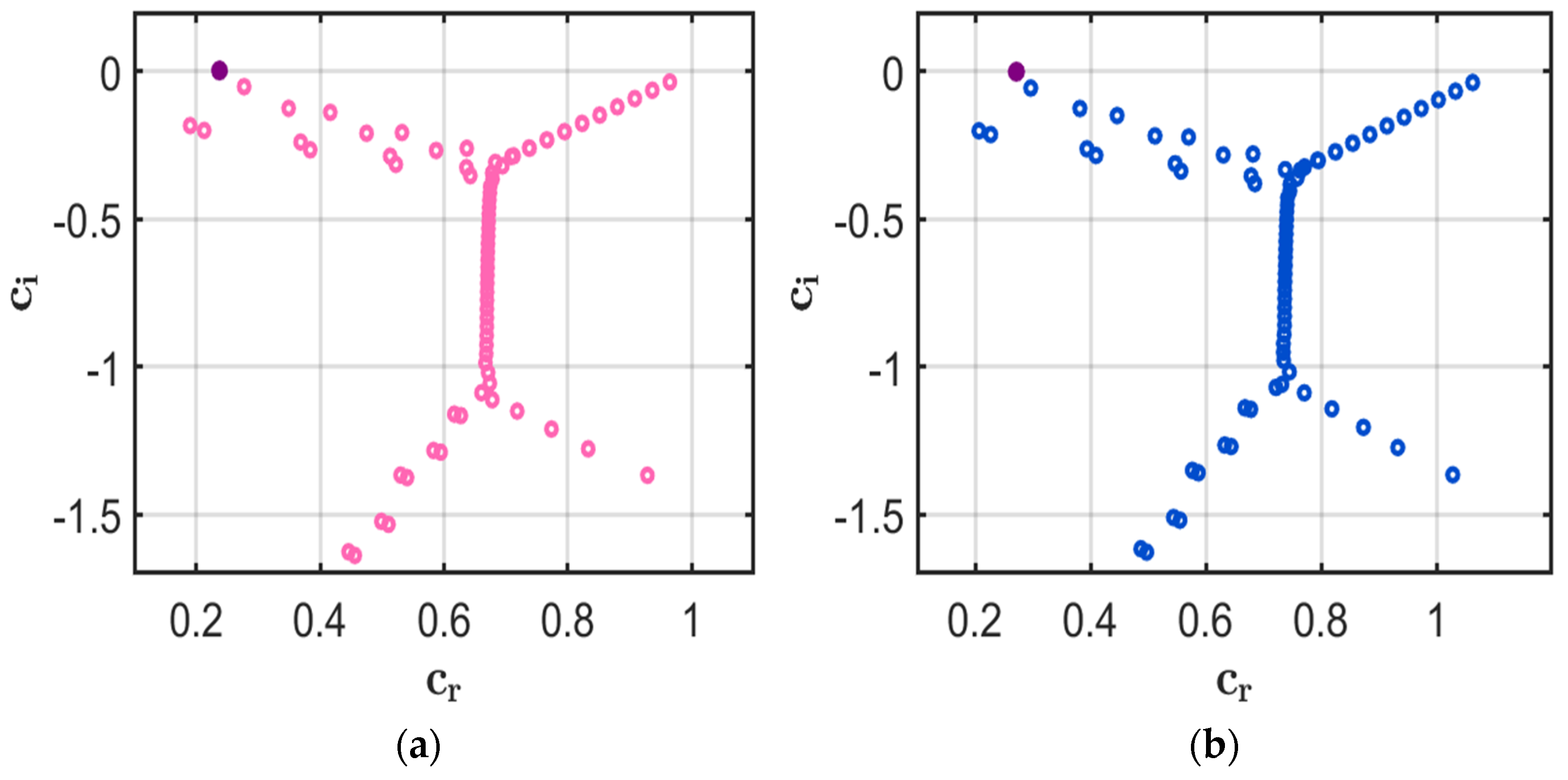
Figure 14 compares the eigenvalue spectra for the smooth- and rough-wall configurations. As shown in Figure 14a, several eigenvalues lie in the unstable region $\left(c_i>0\right)$, indicating disturbance growth. In contrast, the rough-wall configuration in Figure 14b shifts the eigenvalues toward the stable region $\left(c_i<0\right)$, demonstrating a stabilising effect within the considered parameter range. This result indicates that surface roughness modifies the disturbance characteristics and suppresses the growth of the unstable modes under the present no-slip boundary conditions. Furthermore, increasing the roughness wavenumber strengthens the observed stabilising effect, as reflected by the further shift in the relevant eigenvalues toward the stable region.

Figure 14. Eigenvalue spectra for plane Poiseuille flow in the limiting case $Da\to \infty$ and Ha = 0. (a) k = 0. (b) k = 0.1.

Table 10 compares the most unstable eigenvalue obtained using the present Chebyshev spectral collocation method with the benchmark solution of Orszag [31] for $Re=\mathrm{10,000}$ and $\alpha =1.0$. The results show excellent agreement, confirming the accuracy of the present numerical method. As the number of Chebyshev collocation points ($N$) increases, the computed eigenvalues converge rapidly to the benchmark solution. Good agreement is achieved at $N=50$, demonstrating the spectral convergence and numerical reliability of the proposed approach.

Table 10. The most unstable eigenvalue c for Re = 10,000, α = 1.0 and different values of N.

N	c (Orszag [31])	c (Present Results)
20	0.23752 + 0.003734i	0.23801 + 0.003299i
23	0.23752 + 0.003739i	0.23635 + 0.001255i
26	0.23752 + 0.003739i	0.23743 + 0.004788i
29	0.23752 + 0.003739i	0.23739+ 0.003750i
32	0.23752 + 0.003739i	0.23748 + 0.003641i
38	0.23752 + 0.003739i	0.23750 + 0.003750i
50	0.23752 + 0.003739i	0.23752 + 0.003739i

Table 11 presents the spectral convergence of the most unstable eigenvalue as the number of Chebyshev collocation points increases. The results demonstrate that both the real and imaginary parts of the eigenvalue converge rapidly as $N$ increases, with negligible variation for $N\ge 70$. The corresponding relative errors also decrease significantly, confirming the numerical convergence of the discretised Orr–Sommerfeld eigenvalue problem. Based on this convergence assessment, $N=120$ is adopted for all subsequent stability calculations.

Table 11. Spectral convergence of the most unstable eigenvalue for $Re=\mathrm{10,000}$, G = 2, and α = 1.0.

N	cr	ci	Relative Error in cr (%)	Relative Error in ci (%)
30	0.23742	0.00376	0.04142	0.8040
40	0.23751	0.00373	0.00376	0.2394
50	0.23752	0.00373	0.00008	0.01332
60	0.23752	0.00373	≈0	0.00017
80	0.23752	0.00373	≈0	≈0
100	0.23752	0.00373	≈0	≈0
120	0.23752	0.00373	≈0	≈0

Table 12 compares the critical stability parameters for smooth- and rough-wall plane Poiseuille flow. For the smooth-wall case ($k=0$), the computed critical values are in excellent agreement with the benchmark solution of Orszag [31], confirming the validity of the present stability formulation.

Table 12. Critical values for plane Poiseuille flow with $G=2,N=120.$

k	Rec	αc	c
0	5772.22	1.02	0.26400 + 0.00000i
0.1	5889.97	1.0	0.27973 + 0.00000i

For the rough-wall case $k=0.1$, the critical Reynolds number increases to $\mathrm{R}{\mathrm{e}}_{\mathrm{c}}=5889.97$, indicating that a higher Reynolds number is required for the onset of instability. This result demonstrates that surface roughness delays transition in the present configuration. The increase in the critical Reynolds number indicates that surface roughness has a stabilising effect within the parameter range considered, requiring a higher Reynolds number for the onset of instability. The corresponding increase in the critical wavenumber, ${\alpha }_c$, further indicates that surface roughness modifies the spatial characteristics of the most unstable disturbance mode.

The critical Reynolds number is determined from the neutral stability condition, $cᵢ=0.$ For each $\alpha$, the eigenvalue with the largest $cᵢ$ is identified as the most unstable mode. The calculations are performed over $0.1\le \alpha \le 5.0$ and $500\le Re\le \mathrm{20,000}$. The critical Reynolds number, $R{e}_c$, is defined as the minimum Reynolds number on the neutral stability curve, with the corresponding wavenumber denoted by ${\alpha }_c.$

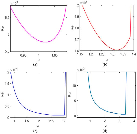
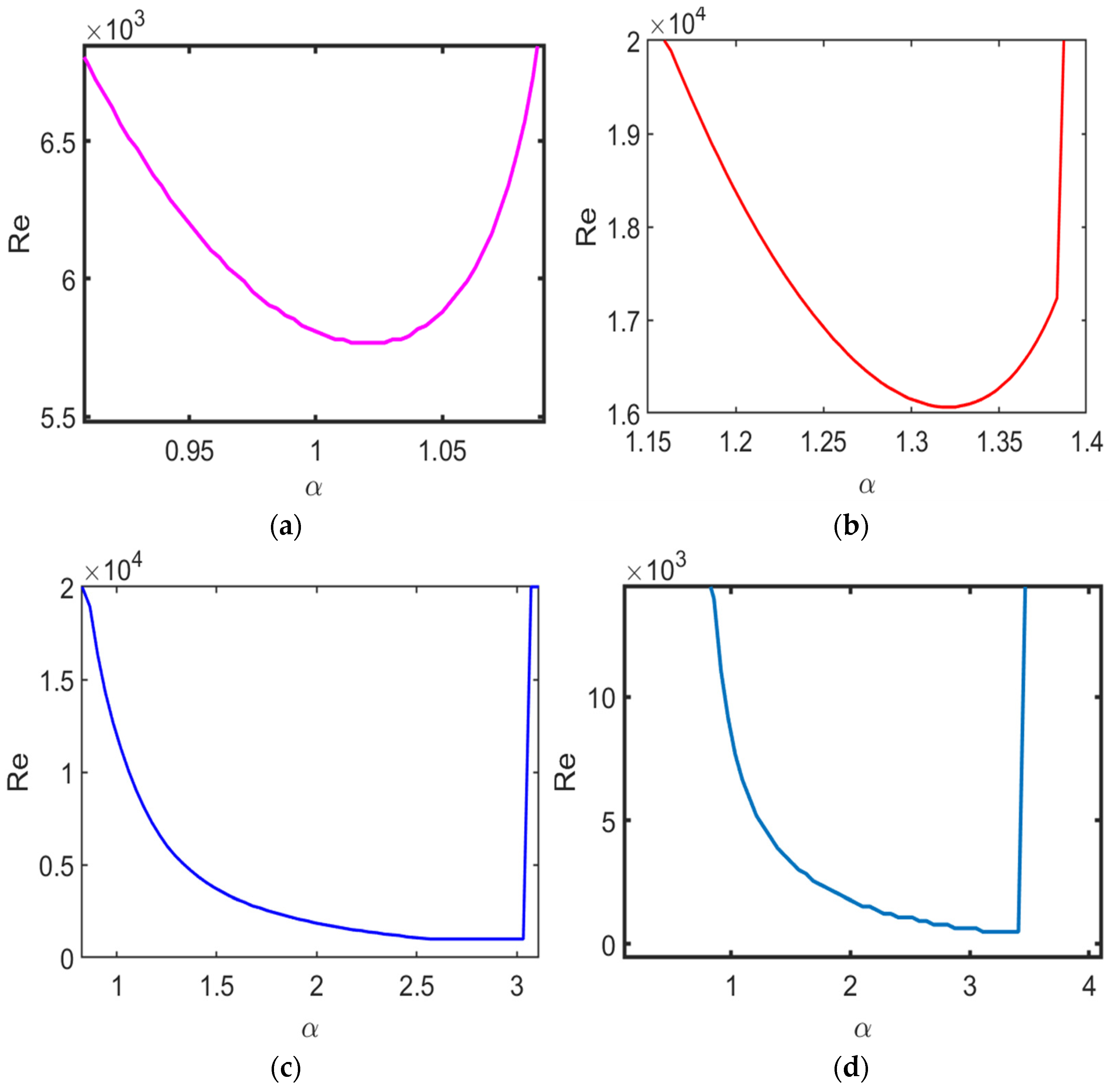
Figure 15 compares neutral stability curves for different channel-flow configurations, demonstrating how both wall slip and wall roughness influence the onset of flow instability. For all cases, the Reynolds number is considered in the range $1000\le Re\le \mathrm{20,000}$, while the disturbance wavenumber is varied over $0.2\le \alpha \le 5$. The same Reynolds-number and wavenumber ranges are used consistently in all cases to facilitate direct comparison of the neutral stability characteristics. Neutral stability curves represent the boundary between the stable and unstable regimes, where the temporal growth rate of the disturbance is zero.

Figure 15. Neutral stability curves for different boundary configurations (G = 2, N = 120). (a) Poiseuille flow. (b) No-slip walls with a rough lower wall (k = 0.1), Da = Ha = 1. (c) Upper wall slip (λ = 0.1) with a rough lower wall (k = 0.1), Da = Ha = 1. (d) Slip at both walls (λ₁ = λ₂ = 0.1) with a rough lower wall (k = 0.1), Da = Ha = 1.

Figure 15a corresponds to plane Poiseuille flow. The neutral curve reaches its minimum value at approximately $R{e}_c\approx 5772$, which agrees well with the classical result. Figure 15b demonstrates the shift of the neutral curve to higher Reynolds numbers due to the presence of surface roughness. The shift of the neutral stability curve toward higher Reynolds numbers indicates that a higher Reynolds number is required for the onset of instability, demonstrating the stabilising effect of surface roughness within the parameter range considered.

The neutral stability curves of channel flows subject to slip and lower-wall roughness are illustrated in Figure 15c,d. Both curves are shifted toward lower Reynolds numbers compared with the rough no-slip channel, indicating an earlier onset of instability. This shift demonstrates that wall slip has a destabilising influence within the considered parameter range. Compared with the configuration shown in Figure 15c, the configuration in Figure 15d exhibits a more pronounced destabilising effect, as evidenced by the further displacement of the neutral stability curve toward lower Reynolds numbers. These results indicate that stability characteristics are strongly influenced by the combined effects of wall slip and surface roughness.

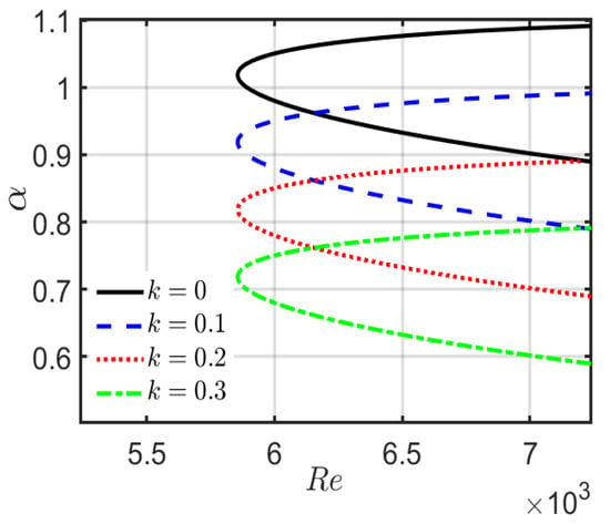
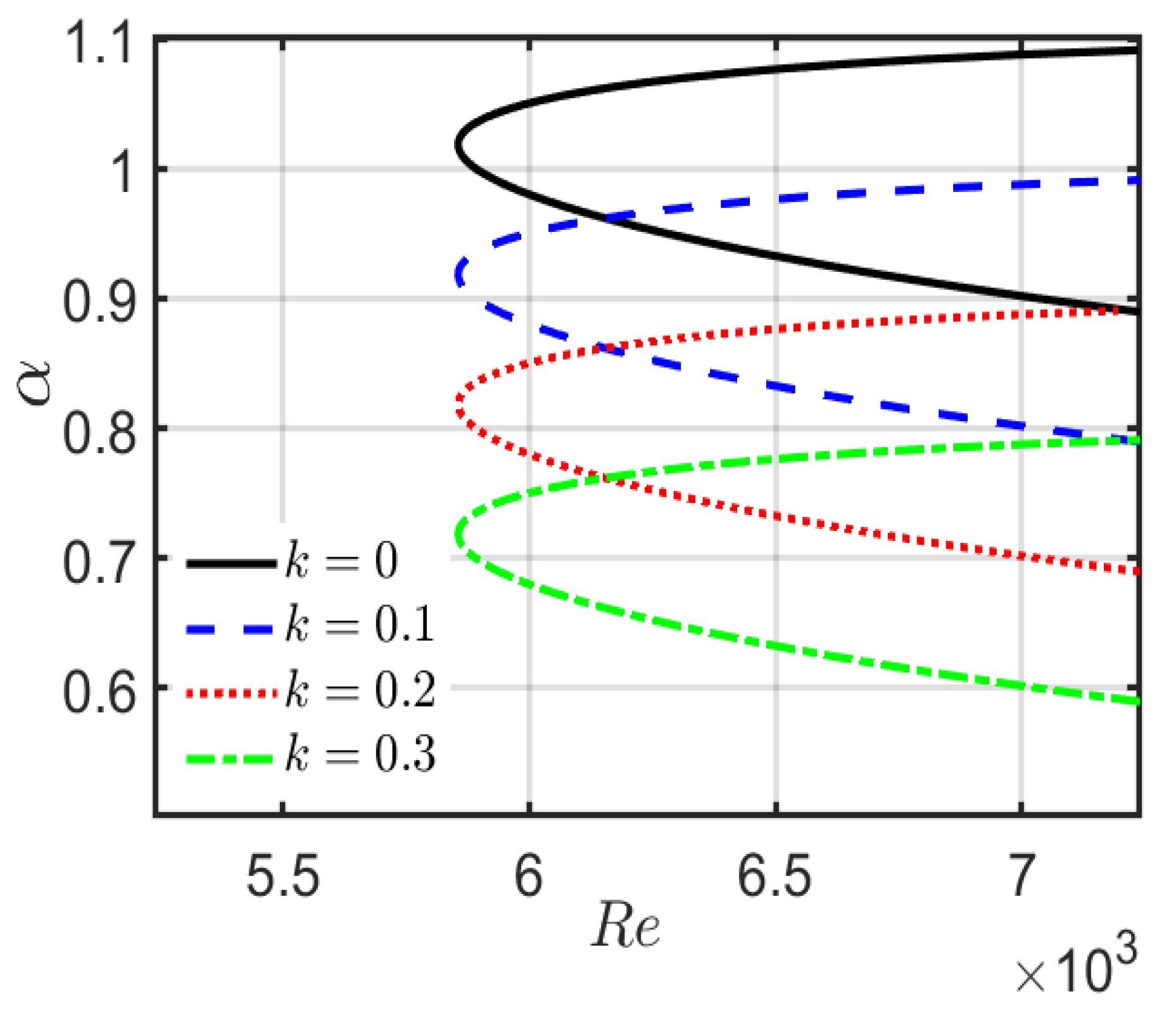
Figure 16 illustrates the neutral stability characteristics of classical plane Poiseuille flow for surface roughness wavenumbers $k=0, 0.1, 0.2,$ and $0.3.$ The smooth-wall case $\left(k=0\right)$ provides the reference stability boundary. As the roughness wavenumber increases, the neutral stability curves shift systematically toward lower disturbance wavenumbers, while the critical Reynolds number remains comparatively insensitive to $k.$ This indicates that the roughness wavenumber primarily modifies the critical disturbance characteristics. The overall trend and ordering of the neutral stability curves are qualitatively consistent with those reported by Zhang and Zhang [16], providing additional validation of the present rough-wall formulation.

Figure 16. Neutral stability curves of classical plane Poiseuille flow for different surface roughness wavenumbers (k = 0, 0.1, 0.2, 0.3).

The present stability analysis is relevant to electrically conducting fluid flows through porous channels subjected to an externally applied magnetic field, where wall slip and surface irregularities may influence the flow behaviour. Such configurations arise in porous-media transport, electromagnetic flow-control systems, filtration and separation processes, and thermal-management applications involving electrically conducting fluids. The present results provide a theoretical assessment of how magnetic-field strength, porous-medium permeability, wall slip, and surface roughness affect the base-flow characteristics and linear disturbance stability. The model can therefore be used to identify stability trends and parameter regimes relevant to the design and operation of porous-channel flow systems.

The present analysis assumes that the periodically corrugated lower wall represents a small-amplitude geometric perturbation and does not alter the bulk permeability $K$ of the porous medium. This assumption is consistent with the adopted homogenised Darcy–Brinkman framework for small wall deformations. For sufficiently large $Da$, however, the pore and channel length scales may become comparable, and the homogenised description becomes less representative. The corresponding large-$Da$ results are therefore interpreted as mathematical trends of the model rather than direct predictions for a particular porous material.

The present study is based on two-dimensional linear temporal stability analysis. It does not include a separate disturbance-energy-budget analysis. Accordingly, the physical interpretations are restricted to the effects directly supported by the governing equations, base-flow profiles, and computed eigenvalue spectra. The analysis also considers small-amplitude sinusoidal roughness and the adopted single-sideband approximation. A detailed disturbance-energy analysis, together with nonlinear, three-dimensional, and fully coupled roughness effects, will be considered in future work.

6. Conclusions

In this study, the linear stability of magnetohydrodynamic flow through a porous channel with Navier-slip boundary conditions and lower-wall surface roughness is investigated using a roughness-modified Orr–Sommerfeld formulation solved using the Chebyshev spectral collocation method. The principal findings are summarised as follows:

• Increasing the roughness wavenumber enhances flow stability by increasing disturbance attenuation while producing negligible changes in the base-flow velocity.
• Wall slip increases the base-flow velocity and suppresses disturbance growth, demonstrating that reduced wall shear resistance can enhance the temporal stability of the flow within the investigated range.
• Increasing the Darcy number promotes instability by reducing porous-medium resistance, thereby increasing the disturbance growth rate and altering the flow’s stability characteristics.
• Magnetic-field strength provides a strong stabilising mechanism through Lorentz-force damping, progressively suppressing disturbance growth and shifting the dominant eigenvalues toward the stable region.
• The proposed numerical formulation accurately captures the stability characteristics of MHD porous-channel flow and provides consistent results for the limiting classical configuration, supporting the validity of the present formulation.

The findings provide useful insights for controlling flow stability in applications such as microfluidic devices, porous-channel systems, electromagnetic flow control, filtration, and lubrication.

References

- Navier, C.L.M.H. Mémoire sur les lois du mouvement des fluides. Mém. l’Académie R. Des. Sci. l’Institut Fr. 1823, 6, 389–440. [Google Scholar]
- He, Q.; Wang, X. The effect of the boundary slip on the stability of shear flow. ZAMM-J. Appl. Math. Mech./Zeitschrift Für Angew. Math. Mech. 2008, 88, 729–734. [Google Scholar] [CrossRef] [Scilit]
- Makinde, O.D.; Mhone, P.Y. On Temporal Stability Analysis for Hydromagnetic Flow in a Channel Filled with a Saturated Porous Medium. Flow Turbul. Combust. 2009, 83, 21–32. [Google Scholar] [CrossRef] [Scilit]
- Smolentsev, S. MHD duct flows under hydrodynamic ‘slip’ condition. Theor. Comput. Fluid Dyn. 2009, 23, 557–570. [Google Scholar] [CrossRef] [Scilit]
- Bhat, A.; Katagi, N.N.; Bujurke, N.M. Analysis of laminar flow in a porous pipe with slip velocity. J. Mech. Eng. Res. Dev. 2017, 40, 526–536. [Google Scholar]
- Chai, C.; Song, B. Stability of slip channel flow revisited. Phys. Fluids 2019, 31, 084105. [Google Scholar] [CrossRef] [Scilit]
- Ceccacci, S.; Calabretto, S.A.W.; Thomas, C.; Denier, J.P. The linear stability of slip channel flows. Phys. Fluids 2022, 34, 074103. [Google Scholar] [CrossRef] [Scilit]
- Badday, A.J.; Harfash, A.J. Magnetohydrodynamic instability of fluid flow in a porous channel with slip boundary conditions. Appl. Math. Comput. 2022, 432, 127363. [Google Scholar] [CrossRef] [Scilit]
- Dabiri, J.O.; Leonard, A. Linear instability of viscous parallel shear flows: Revisiting the perturbation no-slip condition. J. Fluid Mech. 2024, 996, A47. [Google Scholar] [CrossRef] [Scilit]
- Yadav, P.K.; Srivastava, P. Impact of porous material and slip condition on the MHD flow of immiscible Couple stress-Newtonian fluids through an inclined channel: Head loss and pressure difference. Chin. J. Phys. 2024, 89, 1198–1221. [Google Scholar] [CrossRef] [Scilit]
- Kudenatti, R.B.; Bharathi, M.C.; Noor-E-Misbah. Linear stability on transpiration effect of self-similar boundary layer flow for non-Newtonian fluids over a moving wedge. Math. Comput. Simul. 2025, 231, 46–61. [Google Scholar] [CrossRef] [Scilit]
- Geetha, D.L.; Shivaraj, D.L. Stability of Plane Poiseuille Channel Flow of a Classical Newtonian Fluid in the Presence of Uniform Transverse Magnetic Field: Modal and Non-modal Approach. In Innovative Solutions: A Systematic Approach Towards Sustainable Future, 1st ed.; BP International: West Bengal, India, 2025; pp. 317–331. [Google Scholar] [CrossRef] [Scilit]
- Shivaraj, D.L.; Geetha, D.L.; Basavaraj, M.S. Modal and Nonmodal Instabilities of a Two-Dimensional Channel Flow Subject to Wall Slip and Transverse Magnetic Field. J. Fluids Eng. 2025, 147, 091301. [Google Scholar] [CrossRef] [Scilit]
- Arjun, C.M.; Praveena, M.M.; Gogate, S.S.P.; Bharathi, M.C. Linear stability of Navier–Stokes–Voigt fluid under the influence of uniform magnetic field in a porous medium. Int. J. Non. Linear. Mech. 2025, 175, 105105. [Google Scholar] [CrossRef] [Scilit]
- Benbeghila, A.; Ouzani, R.; Benderradji, A.; Alloui, Z.; Khelladi, S. Linear stability of Rayleigh-Bénard-Poiseuille flow of water near 4 °C in a channel bounded by slip walls. Int. Commun. Heat Mass Transf. 2025, 160, 108370. [Google Scholar] [CrossRef] [Scilit]
- Zhang, J.; Zhang, R. Linear stability analysis in channel with slippery and rough boundaries. Phys. Fluids 2024, 36, 124110. [Google Scholar] [CrossRef] [Scilit]
- Floryan, J.M. Two-dimensional instability of flow in a rough channel. Phys. Fluids 2005, 17, 044101. [Google Scholar] [CrossRef] [Scilit]
- Floryan, J.M. Three-dimensional instabilities of laminar flow in a rough channel and the concept of hydraulically smooth wall. Eur. J. Mech.-B/Fluids 2007, 26, 305–329. [Google Scholar] [CrossRef] [Scilit]
- Hajool, S.S.; Harfash, A.J. Hydrodynamic stability of Poiseuille flow in a bidisperse porous medium with slip effect. Int. J. Mod. Phys. B 2025, 39, 2550006. [Google Scholar] [CrossRef] [Scilit]
- Mostapha, D.R.; Nabil, T.M.E.; Abbas, W. Nonlinear Analysis of Ion-Slip and Surface Roughness Effects in Peristaltic Flow of Williamson Nanofluid Through a Stenosed Artery with Reference to Experimental Observations. J. Nonlinear Math. Phys. 2025, 33, 2. [Google Scholar] [CrossRef] [Scilit]
- Suresha, R.; Hanumagowda, B.N.; Arunkumar, R.; Raghavendra, S. Squeeze film lubrication between a cylinder and a flat porous plate under the influence of magnetohydrodynamics, couple stress, and viscosity variation. Multiscale Multidiscip. Model. Exp. Des. 2026, 9, 104. [Google Scholar] [CrossRef] [Scilit]
- Chhabra, V.; Nishad, C.S.; Vijay, K.G.; Sahni, M. 2D-MHD Brinkman flow around circular cylinders inside a microchannel exhibiting wall roughness. Can. J. Chem. Eng. 2026, 104, 1051–1082. [Google Scholar] [CrossRef] [Scilit]
- Saha, M.; Ghosh, S. On the magnetohydrodynamic instability pattern of an anisotropic porous media flow in a rotating channel. Phys. Fluids 2026, 38, 014122. [Google Scholar] [CrossRef] [Scilit]
- Kudenatti, R.B.; Noor-E-Misbah. The onset of instability in a hydromagnetic channel flow of Casson fluid: The accurate solutions. Appl. Math. Comput. 2023, 436, 127475. [Google Scholar] [CrossRef] [Scilit]
- Amrutha, H.; Gogate, S.S.P.; M.C., B.; Kudenatti, R.B. Linear stability of viscoelastic Walters’ liquid B in a channel in the presence of a magnetic field. Phys. Fluids 2026, 38, 023107. [Google Scholar] [CrossRef] [Scilit]
- Palaiah, A.P.; Katagi, N.N.; Bhat, A.; Shettar, M. Influence of navier-slip boundary conditions, magnetic field, and porous medium on the stability of two-dimensional channel flow. Sci. Rep. 2026, 16, 14251. [Google Scholar] [CrossRef] [Scilit] [PubMed]
- Bharathi, M.C.; Kudenatti, R.B. Linear stability of channel Poiseuille flow of viscoelastic Giesekus fluid. Proc. R. Soc. A Math. Phys. Eng. Sci. 2025, 481, 20240241. [Google Scholar] [CrossRef] [Scilit]
- Arjun, C.M.; Praveena, M.M.; Gogate, S.S.P. Stability of Plane Poiseuille Flow of Casson Fluid Through a Porous Medium With Magnetic and Slip Effects. J. Fluids Eng. 2026, 148, 20240241. [Google Scholar] [CrossRef] [Scilit]
- Drazin, P.G.; Reid, W.H. Hydrodynamic Stability; Cambridge University Press: Cambridge, UK, 2004. [Google Scholar]
- Trefethen, L.N. Spectral Methods in MATLAB; Society for Industrial and Applied Mathematics: Philadelphia, PA, USA, 2000. [Google Scholar]
- Orszag, S.A. Accurate solution of the Orr–Sommerfeld stability equation. J. Fluid Mech. 1971, 50, 689–703. [Google Scholar] [CrossRef] [Scilit]
Disclaimer/Publisher’s Note: The statements, opinions and data contained in all publications are solely those of the individual author(s) and contributor(s) and not of MDPI and/or the editor(s). MDPI and/or the editor(s) disclaim responsibility for any injury to people or property resulting from any ideas, methods, instructions or products referred to in the content. |
© 2026 by the authors. Licensee MDPI, Basel, Switzerland. This article is an open access article distributed under the terms and conditions of the Creative Commons Attribution (CC BY) license.