


Abstract
Electro-optical bunch arrival time measurement is a method to monitor the timing of bunches in predominantly linear electron accelerators to below femtosecond precision. Despite the method being well established, a stable and fully available measurement was reported only recently. DESY’s free-electron lasers FLASH and EuXFEL feature Bunch Arrival Time (BAM) diagnostics that serve as a standard operation data source for the facility’s longitudinal fast and slow stabilization, as well as an instrument available to the users for pump laser alignment and offline analysis. A comprehensive upgrade and R&D effort targeting the performance of DESY’s BAM was carried out in recent years. The complexity of the device poses challenges to its control layer, calibration, drift control, and operation setup. Solving these proved to be essential in reaching operational stability and high availability. We report on the updates to the BAM controls and the development of automation of numerous tasks that contributed a great deal to achieving long-term stability and full run availability.
1. Introduction
The Free Electron Lasers (FEL) are linear electron accelerators functioning as sources of coherent and intense X-ray light, used for imaging and experiments in a wide range of sciences. One of the key features of the linear electron machines is their longitudinal phase space stability and its control, i.e., the ability to achieve and control precise timing of the generated X-ray pulses. Feedback loops that utilize accelerating cavities located before dispersive sections as actuators, arrival time measurement devices as sensors, and large synchronization networks can stabilize the timing of the machine actively [1] to the level of a few fs [2].
While the control of accelerating cavities and stable reference synchronization networks have been available [3], a stable and highly available sensor that would support weeks or months of undisturbed operation was not, mainly due to its complexity. Targeted R&D effort on the BAM device and its controls at DESY yielded results in the form of providing EuXFEL [4] and FLASH [5] with Bunch Arrival Time (BAM) monitors of high stability and reliability that function as standard machine diagnostics and drive the feedback loops on a daily basis.
This paper describes the results of the R&D effort on the device control level, which proved to be crucial in order to achieve stable and highly available operation. The BAM devices and their electronics require a significant set of configuration and calibration parameters to operate correctly. These parameters can drift or change frequently with electron beam properties, like charge or compression, or with environmental parameters like large humidity fluctuations or tidal effects [6]. The number of devices installed at DESY’s accelerators reached 17. To address reproducibility, stability, and operability of the number of devices, all of the calibration and configuration tasks were automated, and algorithms were developed that replace the necessity of human interaction fully while setting up the system for operation.
1.1. System Description
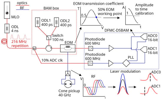
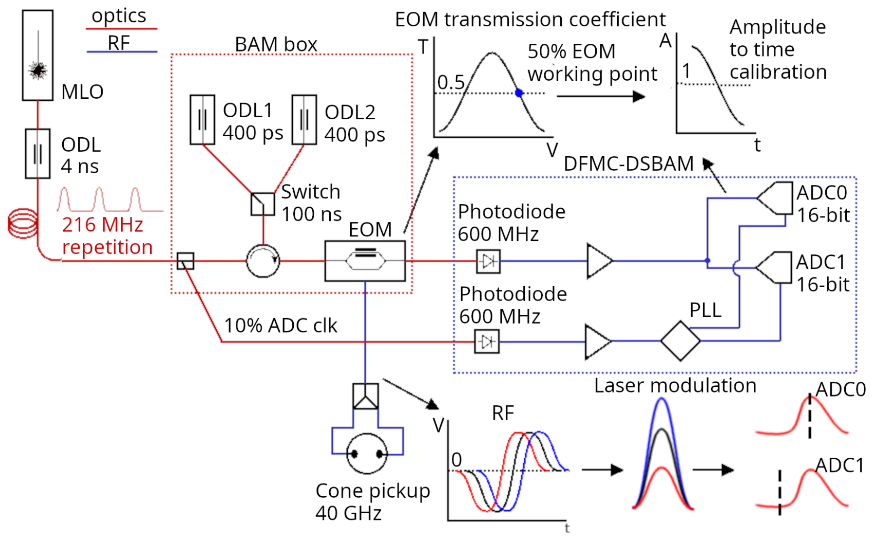
The measurement method of the Bunch Arrival-time Monitor (BAM) utilizes precise laser pulses that sample a bipolar RF signal that is generated by electrons passing a conical pickup. The sampling happens in a Mach–Zehnder Electro-Optical intensity Modulator (EOM) [7]. Thus, phase (or time) information of the bunch arrival time is modulated as the amplitude of the laser pulses to provide a single-shot measurement. A set of multiple devices exists to provide the ecosystem of the measurement, including synchronization, timing, and controls. The BAM itself can be separated into three sub-devices [8]: conical button pickups attached to the vacuum vessel of the accelerator [9]; the measurement device itself located inside a box, called the BAM box, close to the beam pipe and the uTCA readout electronics possibly located farther away. Figure 1 shows the simplified system schematics, including the source of the laser pulses.
Figure 1.
A simplified overall BAM system schematic, showing the device box, readout electronics, and the source Master Laser Oscillator (MLO) and a large Optical Delay Line (ODL) in the synchronization system. The arrows point to the signal shapes. The 50% transmission working point at the top. The RF to optics to ADC samples at the bottom.
The encoding method requires the EOM to be operated at its 50% transmission when no RF signal from the pickups is superposed. The timing is set such that the rising edge of the RF signal is used for the measurement around its zero potential, where its slope is the steepest. The RF signal is bipolar, first negative then positive. Once a passing bunch generates an RF signal, it will superimpose on the 50% transmission of the EOM, leading to relatively increased or decreased transmission, depending on the RF potential at the time when the laser pulse samples it. The laser pulse is an order of magnitude shorter than the rising edge of the RF pulse. Sooner or later bunch arrival leads to higher or lower potential, respectively, at the EOM at the time of the sampling.
The arrival time is then computed with the Equation (1), where is the amplitude of the modulated laser pulse, and is the amplitude of the preceding pulse not modulated with a passing beam. The ratio of / is called “modulation” and reaches values between 0 and 2 for a properly set up system. The calibration function translates the dimensionless modulation value to time units. It is obtained during a calibration process described in Section 2.4.2.
1.1.1. Hardware
The key element of the device, the Mach–Zehnder EOM, is placed in a stabilized and controlled environment, is biased to a proper voltage, and the incoming laser signal is conditioned and delayed with one or two parallel Optical Delay Lines (ODL) to align with the incoming RF signal [8].
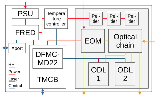
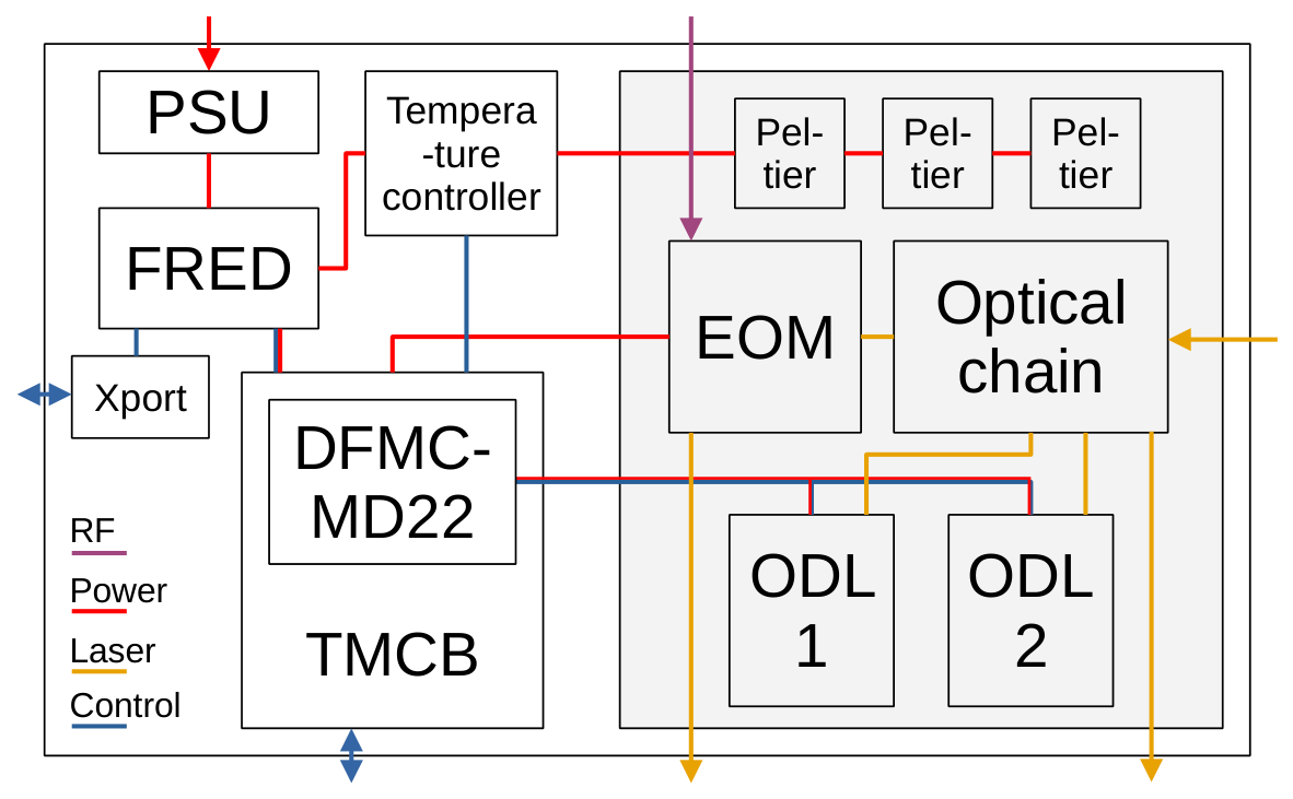
Temperature Monitoring and Control Board (TMCB) electronics act as the control unit of the device box. It is an FPGA carrier with extended connectivity and monitoring functions. It controls a dedicated temperature controller that drives three Peltier elements to provide stable temperature. Furthermore, it hosts a DFMC-MD22 FMC motor driver mezzanine that controls the stepper motors of the ODLs. It also biases the EOM via one of its DACs. Power is supplied from a source via a Fuse Relay Board (FRED) that provides monitoring and power channel control, with the possibility of external control via an Ethernet port (Xport). See Figure 2 for the system schematics.
Figure 2.
System schematics of the BAM box hardware.
1.1.2. Readout Electronics
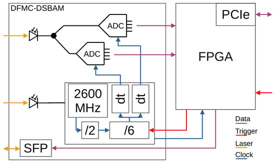
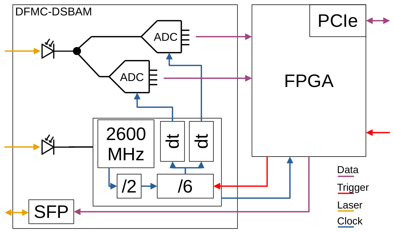
The readout electronics are composed of a uTCA [10] AMC FPGA carrier and an application FMC. DAMC-FMC25 and DFMC-DSBAM v2 are the most prevalent versions installed, while being replaced gradually by the DAMC-FMC2ZUP carrier with DFMC-DSBAM v3 and DFMC-SFP4 mezzanines. The electronics is connect via three optical lines from the BAM box: the modulated bunch signal, the clock signal and the digital control link to the TMCB. The clock and bunch signals are captured with photodiodes at the base MHz repetition rate of the synchronization system. The clock signal drives a clock distribution chip with a PLL. The modulated bunch signal splits into two ADCs and is sampled with the clock generated by the clock distribution chip. The ADCs operate interleaved; one samples the peaks and the other samples the bases of the MHz analog signal. Parallel data links transfer data to the Virtex 5 or UltraScale+ FPGA, where the arrival time is computed. See Figure 3 for the system schematics.
Figure 3.
System and clock distribution schematics of the BAM electronics with DFMC-DSBAM v2.
1.1.3. Software
The software stack for the BAM consists of two servers. They are written in C++ and use the Control System and Hardware Interface with Mapped and Extensible Register-based device Abstraction Tool Kit (ChimeraTK) [11] framework, which allows a control-system middleware-agnostic implementation to enable potential re-use in facilities other than DESY. The servers communicate with each other using the standard control-system communication protocol. The BAM control server is responsible for setting up the DFMC-DSBAM hardware according to fixed setup parameters and persisted online configuration conducted by the operators. It is the main entry point for performing the necessary scans and calibrations to the BAM system as described below. The server also drives the internal ODL to keep the hardware at the optimal operation point. In addition, it publishes the arrival time and derived statistics into the control system for machine operators and beam users to use, as well as diagnostics for the experts.
The second control server, SDM, is a generic control server for managing the TMCB and is also used in other setups for beam diagnostics. Its task is to configure and monitor the temperature controller in the BAM box hardware and provide additional ADC readout and DAC control support. The latter is responsible for generating the bias voltage for the EOM.
2. Materials and Methods
The following sections describe automation algorithms that were developed for the BAM system. The algorithms reside at the software level. The development was conducted in Python 3 using a direct HW or DOOCS interface first, with the majority of the algorithms consequently ported to the principal BAM C++ low-level server based on the ChimeraTK framework. Except for the high-level control, described in Section 2.6, the automation takes place in the software layer in between the hardware and the facility middleware, which is DOOCS [12] in the case of FLASH and EuXFEL. The firmware provides the basic building blocks such as delays, flip-flops, data buffers, and control interfaces but is otherwise transparent to the processing.
The automation algorithms target the hardware configuration described in Section 2.1, the configuration of the back-end electronics described in Section 2.2, alignment with the external systems in the environment described in Section 2.3, and automation of operation described in Section 2.4.
2.1. Hardware Automation
The BAM device hardware is located inside a 4-U (Standard rack unit) high and 19-inch wide box, close to the beam pipe, in order to limit the length of RF cabling that carries the 40 GHz signal from the beam pickups. The main component of the device is the EOM, which requires a biasing voltage and drift control. Devices with two ODLs have an optical switch that distributes the light. Those sensitive components are located within a temperature- and humidity-stabilized compartment.
2.1.1. EOM Bias Voltage
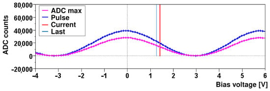
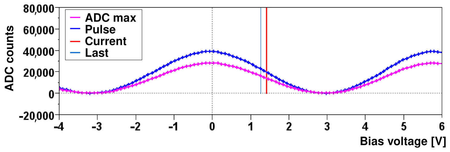
The Mach–Zehnder EOM modulates the passing laser pulses with the RF signal superimposed on a DC bias voltage. BAM is conceived so that zero RF potential produces 50% light transmission, so that the steepest slope of the RF voltage, located around ground, modulates the laser pulses. The location of the 50% point is achieved via a scan shown in Figure 4. A range of ≈4 is scanned with the bias voltage, and a 50% transmission point on the falling edge with rising bias is located. Keeping a falling or rising edge exclusively allows fixing the sign of the relation between arrival time and modulation. A sooner arrival time (more RF voltage at the sampling time) results in less transmission on the falling edge and more transmission on the rising edge. Selection of a 50% point regardless of edge was considered initially, but as it required an additional degree of freedom for calibration function fits Section 2.4.2, it was preferable to fix to one edge.
Figure 4.
One bias voltage scan in the range of −4 to 6 V. Maximum and minimum transmission of the EOM is seen as peaks and bases of the waveform, respectively. The peak sampling ADC is shown as ADC max, and the pulse height (peak-base) is shown as pulse. The current and previous calibration results are marked with the vertical lines.
2.1.2. EOM Bias Drift
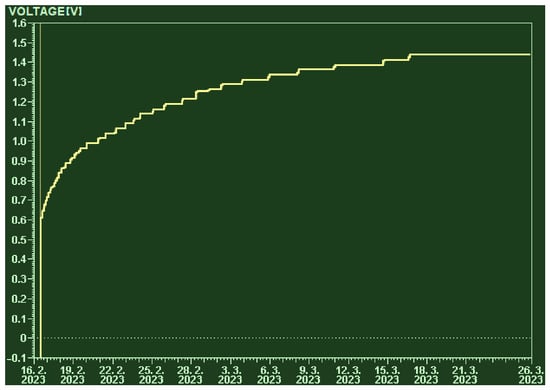
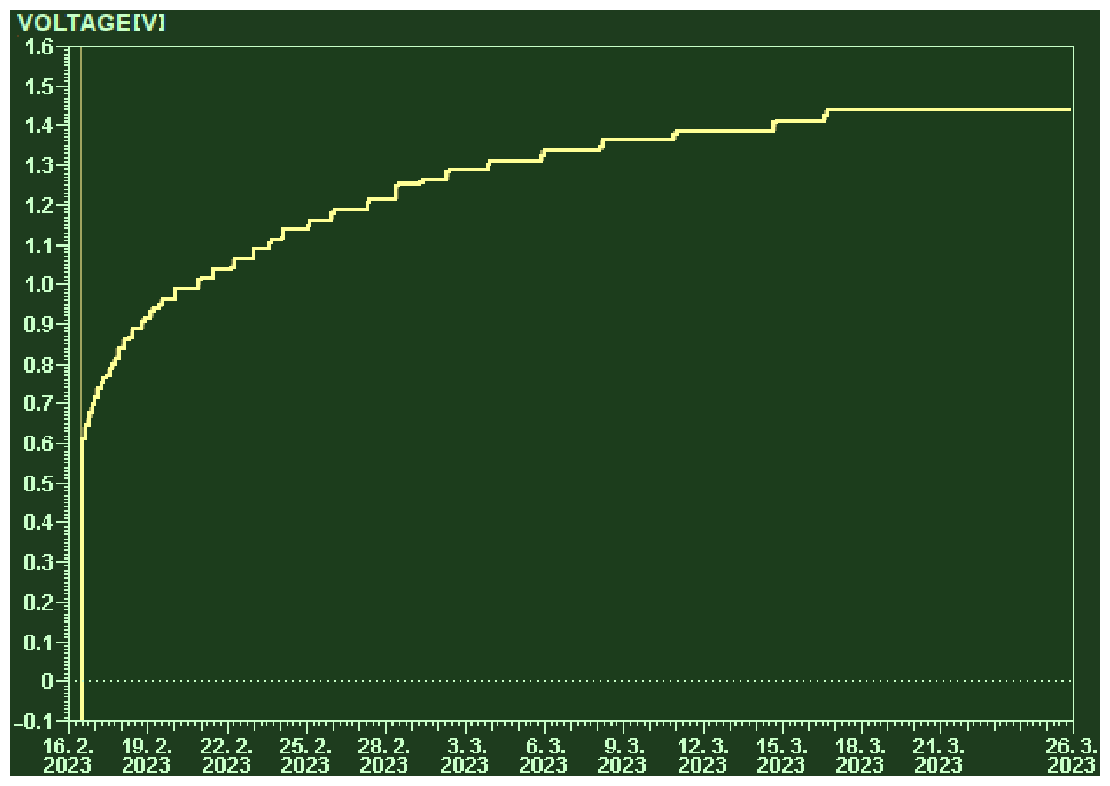
The 50% transmission point described in the previous paragraph is subject to long-term drifts. The drift is strongest after a large change of the bias voltage and decays with time, yet it is still present after days, weeks, or even months in a noticeable magnitude. Such an effect degrades dynamic range and, due to nonlinearities, also the resolution. A proportional feedback that averages a window of 512 laser samples, known to have no RF signal, over several hundred macro-pulses actuates the bias voltage to keep the non-modulated transmission at 50%. The target value is known from the bias voltage scan described in the previous paragraph. Since the drift is strongest after large changes and decays exponentially, the feedback actuating period is set to be one minute after the EOM bias scan for 15 min and is scaled down to 15 min afterwards. Figure 5 shows an example of a bias voltage drift correction.
Figure 5.
Example of EOM 50% transmission biasing drift over a course of one month.
2.1.3. Temperature Stabilization
High sensitivity of the optical components to temperature variations would lead to drifts in the measurement if the temperature were allowed to move freely with the environment or with electronics’ thermal dissipation inside the box. An insulated compartment, heated or cooled with Peltier elements that are controlled by a temperature controller, produces an environment with stability to lower millikelvins. The current strength of the controller was limited to 0.1 A, and the PID algorithm was fine-tuned to avoid temperature controller oscillation and burnouts at power up or down that were observed.
2.1.4. Optical Switch Protection
Two ODLs are installed at stations where large arrival time steps on the beam, in between different RF beam regions, are expected. A fast switch distributes the laser signal between them to accommodate the large step that would reach beyond the range of 1/2 EOM rotation. Switching occurs during accelerator RF transition so that the device is ready for measurement with the following beam region. The switching is triggered by accelerator timing. The switch lifetime is rated in the number of switches in the range of millions. A fault condition in an FPGA or timing configuration can force the switch into fast switching, overheating its control electronics or depleting the switch lifetime fast. A digital protection was built into the switch trigger chain, right before exiting the last FPGA in the chain, to limit the number of switches per second to 100.
2.2. Electronics Automation
The readout electronics feature several clock domains, which have a random relationship between various measurement stations. There is an inherent non-deterministic clock phase generation at the clock distribution chip. The ADC sampling phase requires alignment to the incoming analog signal peaks and bases. All these parameters are, in theory, stable over time. There are drifts in practice, changes in underlying systems that are outside of control, and even a frequent need to reconfirm the setup for especially sensitive measurements, for example. Station configuration was fully automated to combat the complexity and possible drifts and changes. Experience shows that the effort expended on creating the automation was well paid off. The resulting effect is that a station calibrates itself fully with one button click within several minutes, as an alternative to being set up by a human within an hour. The advantage of automation is more evident with scale, in the case of DESY, that being 17 measurement stations. Reproducibility of setpoints generated by software algorithms is also noticeably better than human results. Non-experts can operate the calibration simply, which improves availability in case of recovery from problems. The electronics calibrations are run after shutdowns and interventions, before sensitive measurements, and in case of large drifts in the underlying system.
2.2.1. Clock Digital Delay
The PLL and clock generation chip on the DFMC-DSBAM v2 module does not feature a 0-delay loop. An external, precisely timed signal is required to synchronize its dividers. The PLL’s internal VCO frequency is 2600 MHz, followed by a 2-divider whose phase cannot be controlled, hence booting into one of two possible phases randomly. The 1300 MHz clock is then divided and distributed to outputs. The external signal synchronizes the dividers and must hit outside the metastable regions of the 1300 MHz clock. With the random boot phase of the 2-divider, optimal external signal timing for one phase intersects exactly with the metastable region of the other phase. At such frequencies, internal FPGA latency and jitter, chip-by-chip variation, and thermal effects play a role.
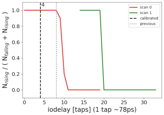
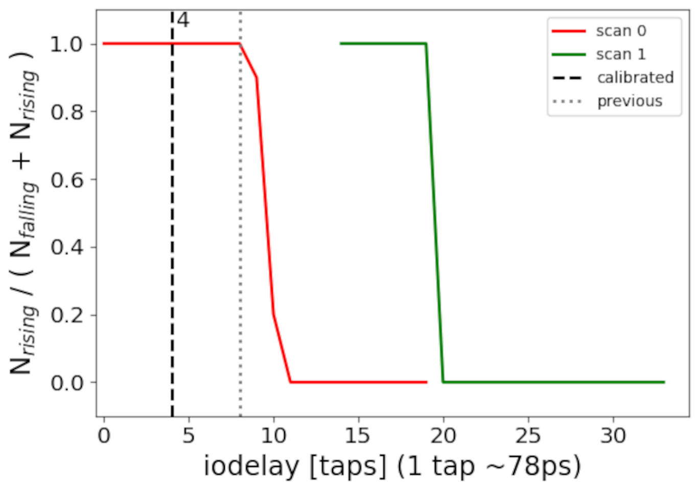
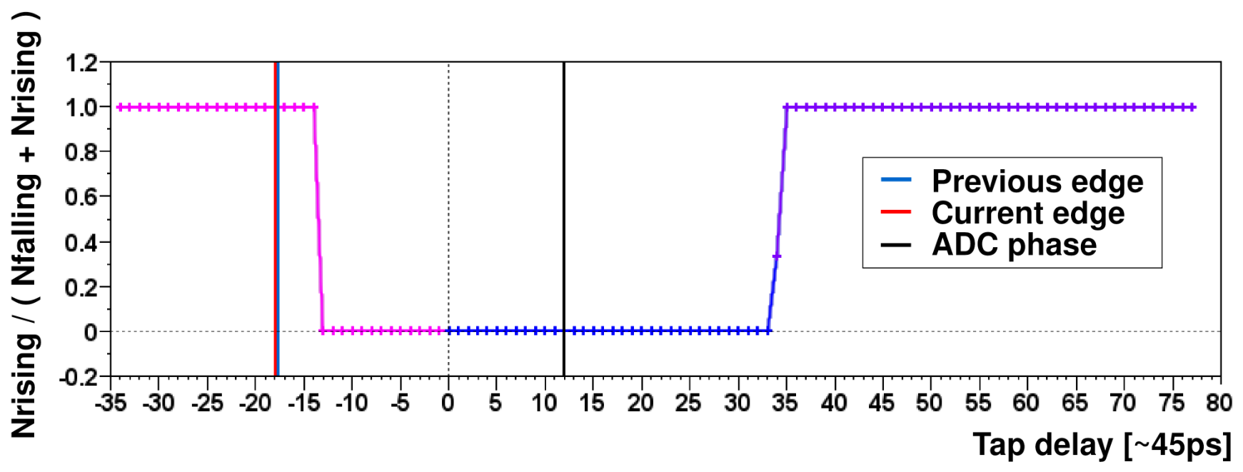
The task is to obtain the internal 1300 MHz clock phase and adjust the synchronization signal accordingly. The developed process uses an external trigger source that is used as a reference to monitor a clock generated by the clock generation chip. The synchronization signal is scanned, and its output delay from the FPGA to the clock generation chip is increased until the metastable region is located and crossed. Crossing the metastable region synchronizes the internal dividers to one 1300 MHz tick later than before. This phase shift of the generated clock, in steps of 1300 MHz, is observed by the external reference trigger. In implementation, the external trigger is sampled by falling- and rising-edge FFs of the generated clock. A phase shift is detected when a trigger signal that is sampled by the rising FF first becomes sampled by the falling FF first. In the first step, stable sampling by the FFs is obtained for the cases when, by chance, the boot-up phase is in metastability, by advancing the synchronization signal and the generated clock until a stable state is reached. In the second step, the generated clock is scanned to locate when the FF sampling precedence toggles. The generated sampling clock is then positioned so that, if the clock dividers slip by one 1300 MHz period, the FF precedence toggles. In the third step, the synchronization signal towards the clock generation chip is scanned until the slip occurs. The internal 1300 MHz clock phase with respect to the synchronization signal is known once the slip occurs. To confirm, steps 2 and 3 are repeated to locate the following slip. Their distance should represent one 1300 MHz period. Figure 6 shows an example of the calibration result.
Figure 6.
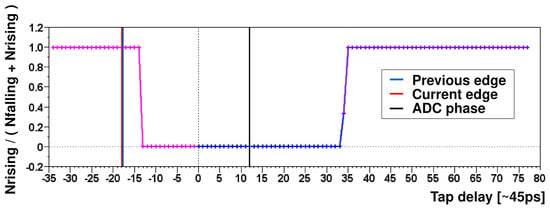
The figure shows a calibration result of obtaining two consecutive slips of dividers inside the clock distribution chip, as the synchronization signal is delayed. The x-axis shows the delay of the generated synchronization signal; the y-axis gives information on which FF sampled the external trigger first, if it was the rising or the falling edge, expressed as a fraction. The displayed scenario shows the previous result to be placed near metastability due to the internal 2-divider starting up in an opposite phase relative to the previous reset.
This calibration step is omitted in the v3 electronics. The hardware design was developed with a 0-delay clock distribution option, which phases the generated clocks to a known and precise relationship always, without the need for an external synchronization trigger.
2.2.2. ADC Sampling Phase
Once a stable synchronization of the clock generation chip is secured, it can be used to align the generated clocks such that the ADCs sample the peak and base of the incoming analog signal.
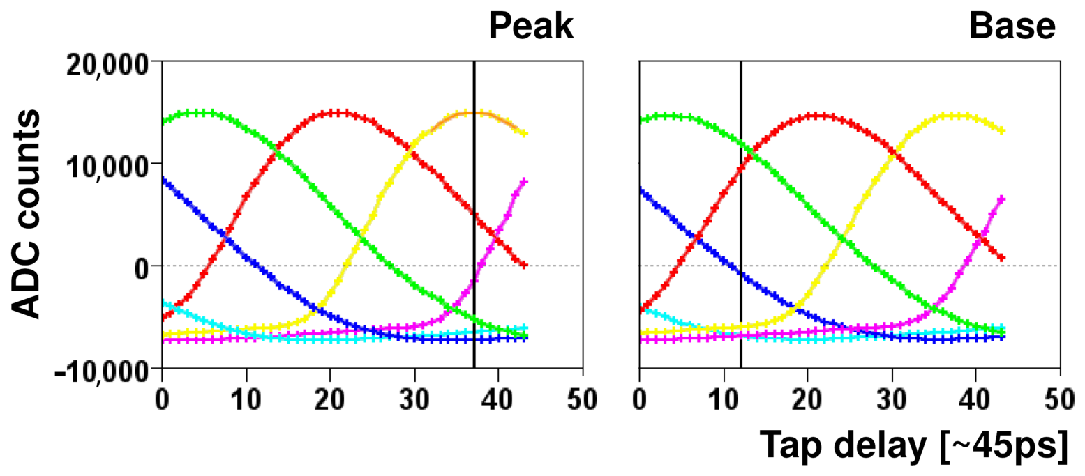
The 1300 MHz divider granularity is aided by the presence of additional tap delay with 45 ps steps. For each of the six divider positions that are possible when dividing by 6 to generate MHz, 44 tap delays are scanned. This results in shifting the ADC sampling phases with respect to the incoming signal, see Figure 7, producing an overlapping signal scan. The PCB layout is such that the ADC sampling the peaks and the ADC sampling the bases is supplied with the same divider. Only the tap delays are independent and thus must be used to set the relative phase of the two. This setup is non-ideal because the tap delays induce clock jitter.
Figure 7.
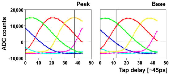
One ADC phase scan of the two interleaving peak and base sampling ADCs. Sampling clock phases of the interleaving ADCs that sample peaks and bases are scanned in 6 coarse (represented by the various colors) and 44 fine steps. Peak sampling is located with signal fitting such that base sampling can be offset by a constant on the same coarse delay waveform (yellow in this case, marked with vertical markers), which is a limitation of the used clock distribution chip.
An existing algorithm that was unstable due to the missing PLL phase control, which is described in Section 2.2.1, was improved and automated. To minimize the effect of the tap delay jitter, the peak sampling phase is selected by locating the divider phase that shows the peak maximum with minimal tap delays that are needed to still provide the base sampling clock with low or zero taps. The maximum of the analog signal is located, and the peak is fitted with a curve to minimize noise effects, and the closest tap delay to the maximum of the fitted curve is selected. The base sampling phase is a constant offset to the peak sampling phase.
2.2.3. Trigger Sampling Phase
An external trigger clock domain provides the bunch selection. The bunches in the machine are represented by the ADC sampling clock domain. The ADC sampling clock drives the data processing; the external trigger is sampled by it. The relative phase of the two must be understood and fixed outside metastability. The existing phase-shifting machinery for the ADC sampling clocks is used to scan the external trigger phase. An identical method utilizing rising and falling FFs is implemented, as for the calibration of the clock generation chip. The trigger phase is located once the precedence of rising/falling flip-flop sampling the incoming trigger changes. If the rising flip-flop samples the trigger first, delaying the sampling clock will eventually result in the falling flip-flop sampling the same signal first. Once the phase is understood, the falling or the rising FF is selected for sampling the external trigger signal, whichever is more distant from the metastability, as shown in Figure 8. There is a possibility to keep the previous result within a window that is considered safe in order to avoid slips in trigger delay in cases where the algorithmic decision can vary between executions due to system jitter.
Figure 8.
Scan to select the trigger sampling flip-flop. The ADC clock is scanned in 3 coarse (even, odd skipped) and 44 fine steps per each to scan (represented by the various colors) over one ADC sampling clock period. Precedence of rising or falling flip-flop sampling of the incoming trigger signal is recorded. The falling edge of the waveform marks where the falling flip-flop is metastable; the rising edge of the flip-flop marks where the rising edge flip-flop is metastable. The algorithm selects the FF whose metastability is farther from the calibrated ADC clock.
2.3. Integration Automation
Two external signal sources are used in the system. One is the trigger signal from the machine timing that aligns the bunch selection. The other is the synchronization signal that provides laser pulses to be modulated by the beam-generated RF signal. Both need to be aligned to the beam at the given measurement station. These calibrations are run rarely because the relationship changes seldom. In practice, only with hardware upgrades in either of the underlying systems.
2.3.1. Trigger Location
The trigger that marks the start of each macropulse is aligned first to place the device data acquisition window in overlap with the beam. Strong ringing follows each bunch signal, spanning over many ADC samples. This is used to locate the trigger. The trigger delay is scanned at source, over a large period of several dozens of milliseconds, until raw ADC data show the large ringing instead of a steady baseline. A standard deviation of a sliding window of 512 ADC samples is used as a baseline, followed by an investigation of a consecutive window of 1024 ADC samples to locate the ringing. The located ringing must be persistent for at least three triggers to discriminate random noise coming from adjacent instrumentation, vacuum pumps, for example. Once located, the first ringing sample is selected as a reference. The selected sample is not necessarily the precise bunch signal, which might be located at one of the adjacent ADC samples. However, the achieved precision is sufficient for coarse trigger delay setup in order to place the beam signal in the data acquisition window.
2.3.2. Beam Signal Location
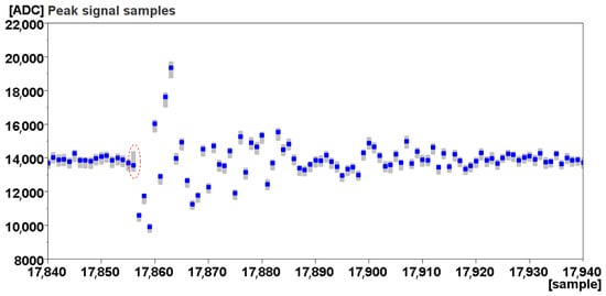
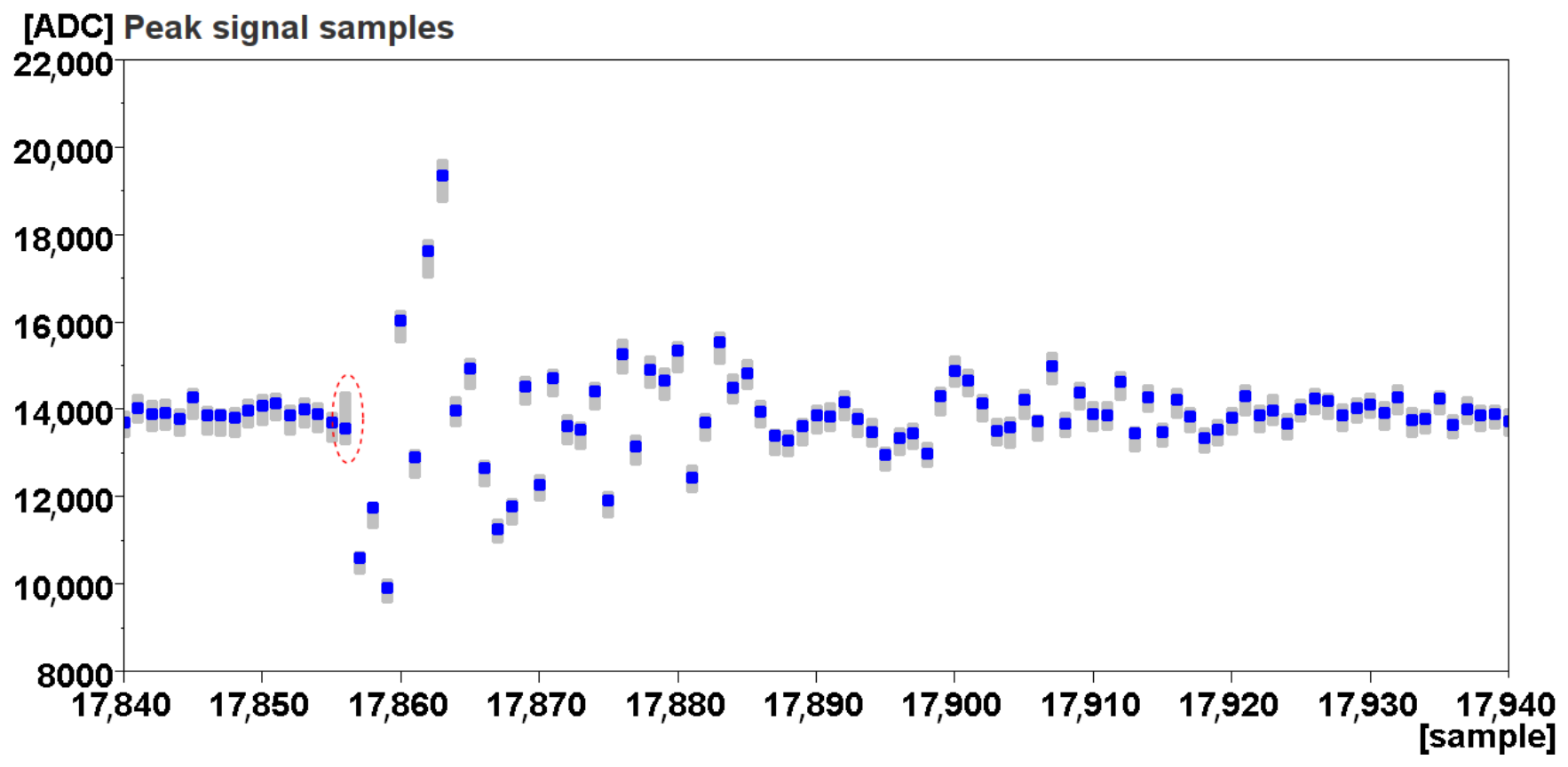
The beam signal position is known to plus or minus several ADC samples after the trigger position was located. An example of a raw ADC signal is shown in Figure 9, with ns granularity. The exact phase of the laser that samples the RF needs to be found with the precision of a few dozen femtoseconds. This is achieved by scanning the sampling laser with ODLs. A large ODL inside the synchronization system is available, spanning almost a full laser repetition period ( ns), that allows for the adjustment. To provide a full period range, a second ODL, also within the synchronization system, is additionally available.
Figure 9.
Raw ADC signal of one bunch sampled with MHz clock (blue data points with grey persistence). It shows a baseline preceding long-term ringing. The highlighted (in red) ADC sample is the modulated sample that measures the arrival time. In this case, the system is well aligned to optimize the measurement sample to baseline level, i.e., the best sensitivity and dynamic range. Its preceding samples are used to acquire the non-modulated baseline.
The task is to scan the ODLs until the start of the characteristic shape of the RF beam signal is located. The complexity comes from the necessity to use two ODLs since one is not enough to scan the whole period. Another complexity comes from the fact that scanning such a large ODL induces a phase shift of the whole BAM electronics with respect to the external timing trigger. This results in metastable trigger sampling at one point and a slip shortly after. For this reason, multiple ADC samples are analyzed at the same time (several samples around the highlighted position on Figure 9).
An initial implementation of the algorithm was aware of the phase relation between the ADC phase and the external trigger that is obtained within trigger calibration (Section 2.2.3). Once the metastable region was approached, the trigger sampling was switched to the opposite edge, and the trigger delay was adjusted by 0 or 1 step to avoid slips. This solution yielded expected results but is rather complicated. A recent solution simply observes the acquired signals and tracks internally any slip resulting from crossing the phases, yielding also reliable results.
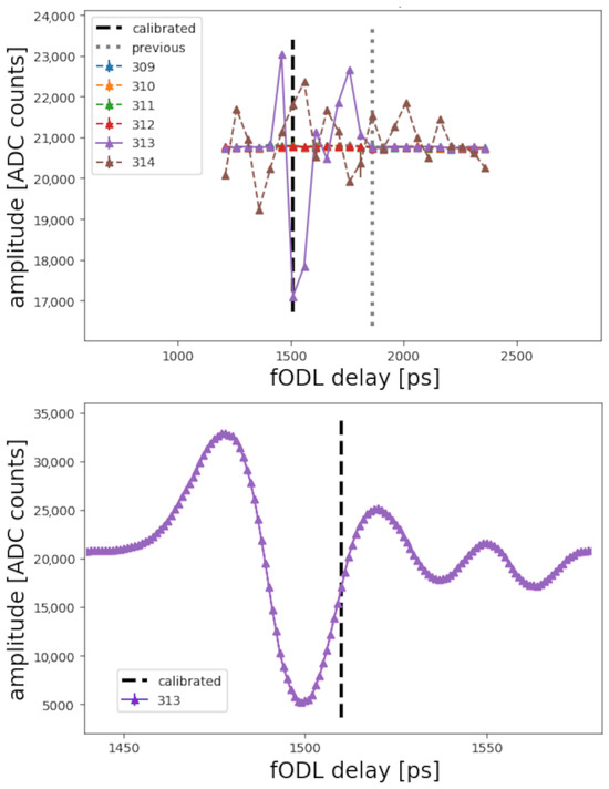
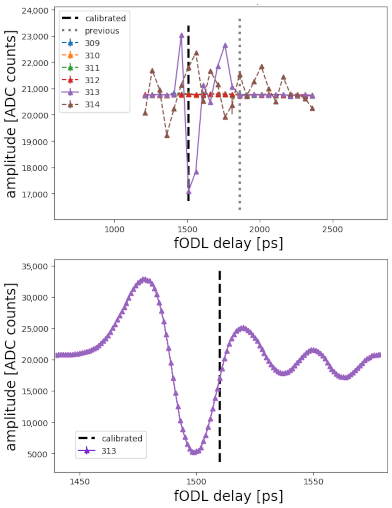
With the ODL moving, the beam signal is located once an ADC sample (one of those on Figure 9) that has been constant starts to oscillate, i.e., to see the RF signal as shown on Figure 10. Alternatively, the beam signal is also located when an oscillating ADC sample becomes constant when scanning in the opposite direction. Coarse location, to several dozen picoseconds, is achieved.
Figure 10.
Scan to locate the RF signal. Several consecutive ADC samples are monitored (numbers 309 to 314 in this case). The sample that shows the start of excitation with RF with increasing ODL delay, in this case number 313, is located. The upper plot shows the overall scan; the lower plot shows a zoom into the located signal.
2.3.3. Precise Trigger Location
A precise trigger signal location is obtained from the previous step (Section 2.3.2) once the exact ADC sample where the RF signal starts oscillating is located. It is, though, possible that after recalibrating the electronics, the new relative phasing of the trigger and ADCs results in a slip by one clock. For cases when the timing system is reconfigured and the trigger shifted, it is advantageous to have a limited algorithm capable of precisely locating the trigger within BAM without moving the large ODLs. This is achieved by scanning the ODL that is internal to the BAM, using a similar algorithm as described in Section 2.4.1. The precise trigger position is located once an ADC sample starts to oscillate with increasing ODL delay.
2.4. Operational Automation
The accelerator machine setup has an effect on the operation point of the BAM. Charge and bunch length influence the RF signal amplitude and steepness. Consequently, the operation point of BAM can move in the range of units of ps and thus outside of the device’s dynamic range, or the calibration of modulation to time can change significantly. These parameters are, therefore, calibrated every time that the machine setup changes. This results in daily or weekly recalibration in practice. The recalibration takes up to two minutes, and is run in parallel for all the stations.
2.4.1. Operation Point Scan
The BAM operates on the first rising RF signal edge of a bipolar RF signal with the negative part first, followed by the positive part. The RF signal modulates the EOM transmission. To achieve higher precision, the RF signal voltage often exceeds the of the EOM; hence, over-rotation is seen on the modulation signal. With decreasing RF potential at the start of the RF signal, the previously increasing transmission starts to decrease as the light phase inside the EOM shifts from destructive interference towards the constructive one.
The internal short ODL is scanned fast and in one step in a range up to 100 ps. The scan is stopped before reaching the whole span if a suitable result is acquired, in order to save time. A non-modulated signal is observed first, followed by the start of modulation, optional over-rotation, the falling edge, and ringing, possibly over-rotated as well. Without over-rotation, the modulation signal is positive where the potential RF is negative. The waveform generated by low charge or a long bunch shows a rather straightforward shape, where the location of the 50% transmission point on the first falling edge of the modulation is uncomplicated. In contrast, the waveform generated by high charge and a short bunch can show several over-rotations and is complicated to analyze algorithmically.
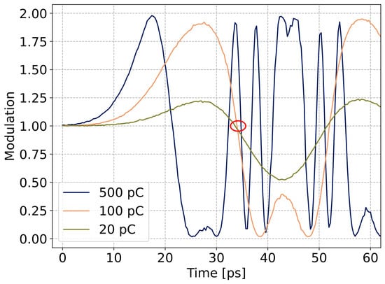
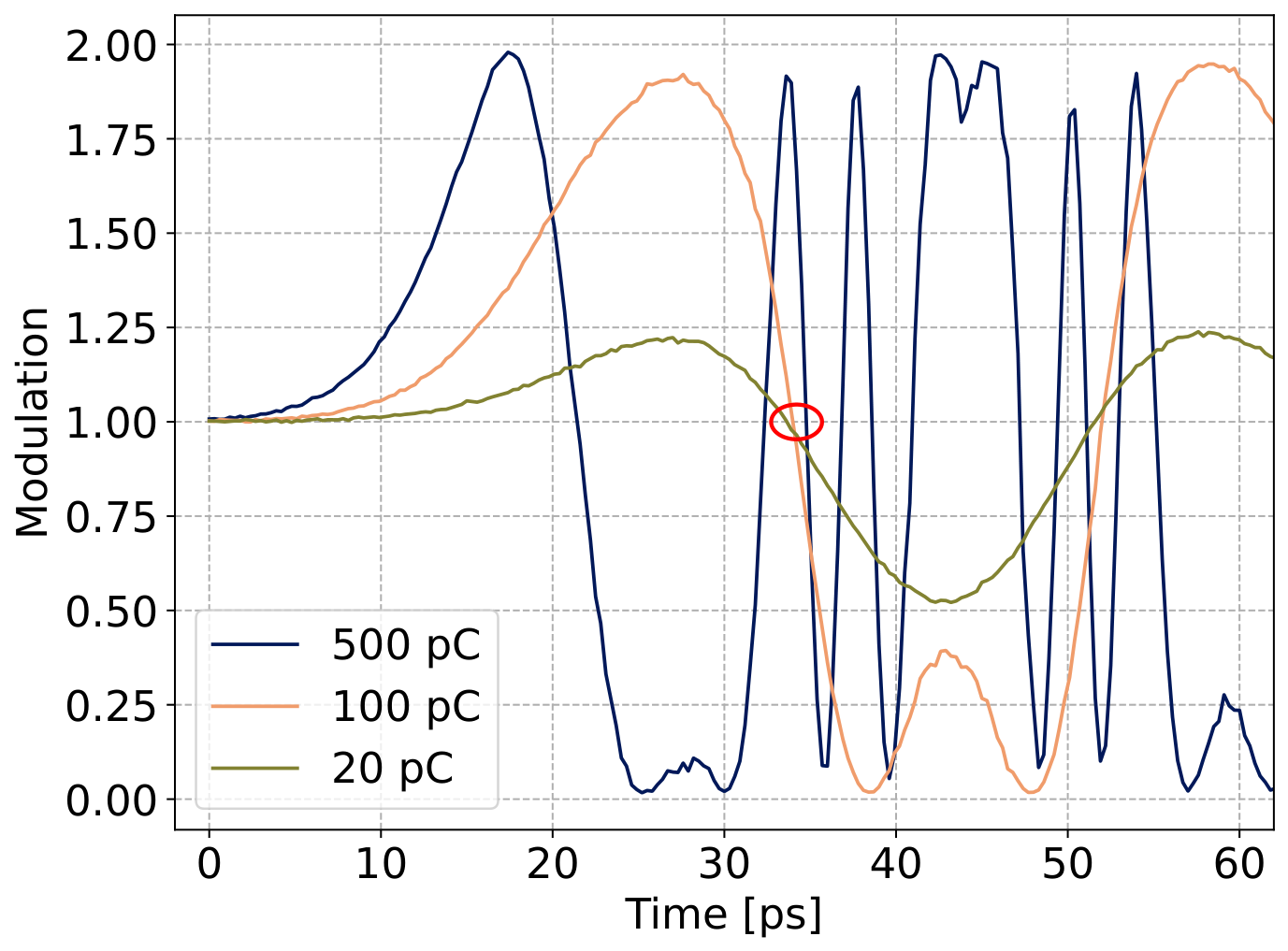
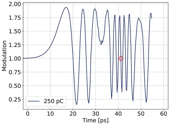
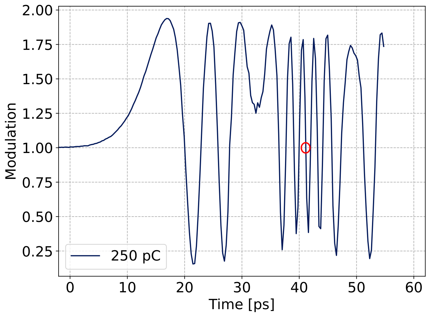
An algorithm with multiple conditions and weights was developed to allow functioning under any of the beam conditions shown in Figure 11 and Figure 12. First, the signal ramp start is located at 1.2 modulation. This is the simplest, but rather imprecise, way to locate a time reference point, as different waveforms cross the point at different phases. Then, points where the waveform crosses the modulation of 1.0 are identified, and their slope is computed. The waveform could be noisy and show local oscillations around the crossing; those are averaged out. A distance window is applied to the located crossings next. Those too early or too late relative to the ramp start are cut. In the following step, inflection points of the waveform are located. For each inflection, its amplitude and distance (width) to the following one is computed. Inflection points with significant noise are also marked. As seen in Figure 12, a convex point with noise and non-extreme amplitude (delay 35 ps) is a good marker for the peak of the RF signal. The inflections are rated using weights in Table 1. Consecutively, all remaining crossings are rated (Table 2). First, up to two top-scoring inflection points are unfolded (over-rotation unfolded) to locate where the fully unfolded signal crosses 1.0. If the inflection amplitudes around the crossing are balanced (similar positive and negative amplitudes), they score extra points. Finally, a steepness score is added. The crossing that scores the most points is selected as the operation point.
Figure 11.
Dependency of modulation waveform on beam charge. The 500 pC curve shows slightly above one fold over modulation. The crossing point shifts later with charge by units of ps, located around 34 ps (in red).
Figure 12.
Modulation waveform generated by a station with a higher RF gain, producing a 4.5-fold over-rotation. The search algorithm locates, also in this case, the operation point at the falling edge at a 41 ps delay (in red).
Table 1.
Inflection points rating.
Table 2.
Crossing points rating.
2.4.2. Calibration
Beam charge and bunch length influence the slope and dynamic range. The more charge and the shorter the bunch, the steeper the operating slope is, providing more resolution and less dynamic range. Additionally, the offset of the slope changes. The internal ODL of BAM is taken as a time reference. Scanning slowly, in steps and with integration, the ODL around the operation point that was obtained in the previous step (Section 2.4.1) provides modulation to the time relationship [8], which is then used as the calibration function in Equation (1).
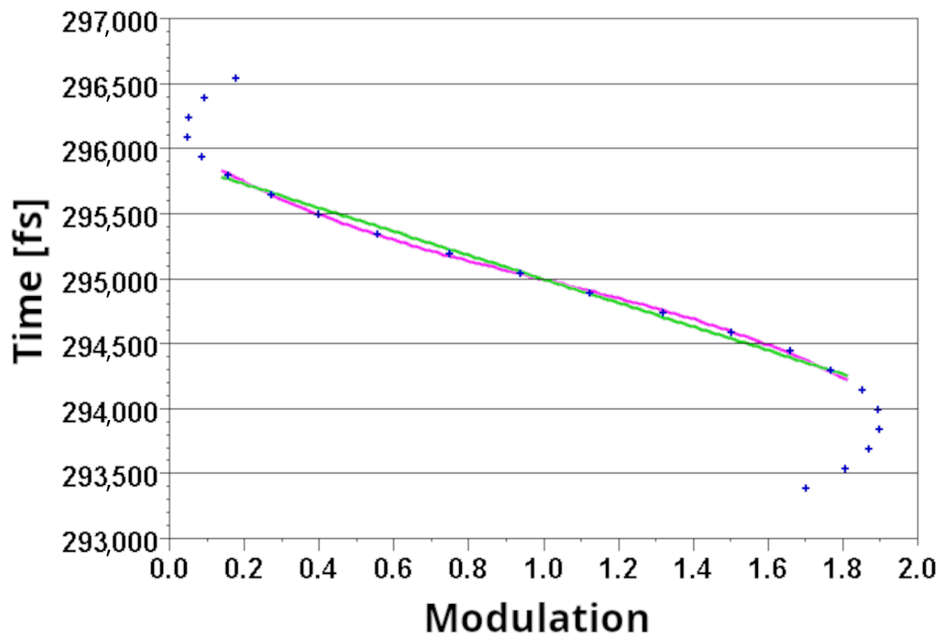
The upgraded algorithm finds the crossing of the no-modulation level (1.0 in absolute value) that is closest to the operation point and explores to the left and right to obtain modulation inflection points, which are usually a maximum and minimum modulation. Once obtained, the range of 0.9 of maximum to 1.1 of minimum is fitted with a fourth-order polynomial to obtain a smooth calibration function. The process is repeated for each RF beam region due to possible different charges or compression of the bunches located in different RF beam regions.
Figure 13 shows details of the calibration scan.
Figure 13.
Calibration of measured modulation to time. One falling edge of the modulation signal is scanned in fine steps and then fit with linear (green) and polynomial (magenta) functions. The axes are swapped with respect to the plots of modulation functions; here the time is on the y-axis.
2.4.3. Optimization
Optimal precision and the widest dynamic range are available if the device is configured to monitor the RF bunch signal close to zero additional modulation in the EOM, i.e., at the bias voltage. Positioning the mean of modulations of all the filled bunches that pass the given device to a no-modulation point (1.0 in absolute value) was found to be a sufficient solution. After an operation point is located and the modulation calibrated, the internal BAM ODL is varied interactively, utilizing the linear fit to the modulation calibration, to position the mean of the measured raw uncalibrated modulation signal close to the absolute value of 1.0.
2.4.4. Motor Feedback
The feedback algorithm tries to keep the raw arrival time ratio in a user-definable range, which is usually or around the 1.0 mark, by adjusting the ODL internal to the BAM box. After a working point calibration, the system is left in a tuned state well within that range, with the feedback enabled. With each beam shot, the algorithm calculates a mean arrival time over all beam regions that are served by a particular ODL and keeps a rolling average over the past ten shots.
The feedback algorithm has a coarse (correction) and a fine (optimization) mode of operation. After the initial correction caused by the detection of an out-of-range event, it will continue to move the ODL towards the new position with full correction steps until the ratio is in the expected range again. This will cause it to switch into fine mode, where it will only use 75% of the step size until the distance it would need to move falls below a 20 fs change threshold. The system is considered tuned afterward. The step size is estimated depending on the average slope of all beam regions, given by Equation (2).
The algorithm can handle the following special conditions:
- The machine parameters changed significantly when the deviation was detected. This will change the initial correction step to be much larger than in the other case, but then try to continue to move back into the expected arrival time ratio range as described above (coarse, then fine movement).
- The feedback moves the working point to the wrong slope. If the arrival time changes in the opposite direction than what was expected, the algorithm considers itself on the wrong slope. It will move the ODL to an offset of the calibrated working point. The offset is derived from the change in charge and compression compared with the operation point scan, Section 2.4.1. It continues to scan the signal in fixed steps until it runs out of the allowed movement range or finds a valid working point. If it fails, it will disable itself and signal the failure to the operators.
- The feedback moves out of its allowable movement range. This triggers the same recovery procedure as described above.
In contrast to the old implementation of the feedback, the calculations are simplified from an IIR filter on the arrival time ratio to simple averaging, which was found to be sufficient. The introduction of the optimization mode allows for reaching smaller deviations from the 1.0 target. Limiting the movement to a plausible movement range now stops the feedback algorithm much earlier than before, avoiding prolonged searches. Combined with the wrong slope detection and the detection of significant machine parameter changes, this made the feedback much more robust and reliable during operation.
2.5. Integration in Software
The server software implements the automation algorithms. It also offers triggers for two sequencer scripts (initial setup script Section 2.5.1 and operation point reset script Section 2.5.2) to run those operations in a proper sequence. The sequencing, in contrast to the automation algorithms themselves, is implemented in Python currently, even though it could be ported to C++ as well. Those triggers are exposed to an operator for their day-to-day use in the case of the operation point reset and to an expert for the initial setup through a single push-button in the control system. Once pushed, the server will run a Python script on itself that will then execute the individual routines via DOOCS calls to the server itself. By maintaining the sequencer scripts alongside the software’s source code in the same version control repository, the risk of deviation between the server’s interface and the sequencer script is minimized. Previously, these operations had to be carried out by an expert following written procedures. This would not only take significantly more time but was also prone to human error by skipping steps or not having the documentation updated to match the software. Automating the procedures not only eliminated the human factor, but it also sped up the initial setup and the reconfiguration after machine changes and made it safe for the latter to be executed by operators.
2.5.1. Initial Setup
The initial setup sequencer is a Python script that sequences the basic firmware initialization, the clock digital delay scan, Section 2.2.1, the ADC sampling phase scan, Section 2.2.2, the trigger sampling phase scan, Section 2.2.3, and finally the EOM bias scan, Section 2.1.1. If all steps succeed, it will enable the EOM drift compensation on the server, Section 2.1.2.
2.5.2. Operation Point Reset
The operation point reset sequencer runs the operation point scan, Section 2.4.1, followed by the calibration, Section 2.4.2, and will trigger the feedback optimization afterward, Section 2.4.3, and finally enable the motor feedback, Section 2.4.4.
2.6. The Longitudinal Feedback Manager
The Longitudinal Feedback Manager is a middle-layer DOOCS server that provides centralized supervision, coordination, and exception handling for the longitudinal feedback loops of the FLASH and EuXFEL facility, including bunch compression (BCM), bunch arrival (BAM) monitors, and the longitudinal intra-bunch-train feedback (L-IBFB). Rather than acting as a controller itself, the manager orchestrates the existing per-section feedback loops: it enforces consistent default settings (e.g., loop averaging), validates monitor–actuator pairings, and checks that various actuator ranges and per-beam-region constraints remain mutually compatible, including adjacent beam regions to support several bunch-train destinations. It handles the start-up and shut-down sequencing of slow and fast loops in the appropriate order, drives auxiliary procedures such as BAM operation point resets (calibrations in Section 2.4). On the exception-handling side, the manager can react to jumps in upstream loops, to failures of individual monitors, and, in particular, to error flags from involved servers, by disabling the affected feedback loops, signaling the condition to operators, and re-enabling the loops once nominal conditions are restored. In this way, the Longitudinal Feedback Manager turns a collection of independent feedback loops into a coherent, monitorable subsystem and is a key building block for high-availability operation of the bunch arrival time monitors and other surrounding higher-level system components.
3. Results
The principal achieved result is the transition of the BAM system from expert-based temporary operation to standard fully available accelerator diagnostics, supported by the stability and ease of the BAM system configuration and its reproducibility. The automated tasks are faster than humans and produce reproducible results. The day-to-day operation of the system was transferred from experts to ordinary machine operators. The overall workload of the operators was reduced to pressing a single button once the machine was set up to prepare and calibrate the whole BAM system for user operation within a few minutes. The content of this process is described in Section 2.4.
A secondary result is the simplification of the device setup after power cycles or interventions, or if confirmation of the setup is required. The workload of an expert was also reduced to a single button click, processing what is described in Section 2.1 and Section 2.2. In practice, any team member or an operator can conduct the task without deeper system knowledge, which improves availability and shortens the loop of correcting various fault conditions.
A tertiary result is also a simplification of the device configuration relative to its environment, which seldom changes, after major hardware interventions in the underlying systems. Automation in the form of scripts was developed and described in Section 2.3.
The amount of workload required to develop and obtain these results is estimated to be roughly one staff-year of standard intensity work.
4. Discussion and Conclusions
Complex accelerator instrumentation systems tend to have complex configuration requirements and procedures. The project leaders may often be tempted to allocate R&D resources to advancing the system performance, rather than its stability and operating comfort. With this paper, we argue that, in the big picture of a system worth many hundreds of thousands of euros, within an ecosystem with a value of millions, it is well worth going the last mile and investing in stabilizing the operation. On the contrary, relative to the hardware costs, the costs of controls R&D are small, and the gain for the facility and its users is noticeable. The scale of the whole system plays a role in cost-benefit analysis; in the case of EuXFEL and FLASH, the invested time that would have to be spent on simply keeping the devices in operation manually is returned within a few years.
The complexity of the task is manageable, as we report here. The requirement to complete the task is an understanding of the device at the system level and parallel experience with its operation to be able to design the appropriate algorithms. Experience with machine operation is beneficial and helps to design processes that fit the given machine procedures or culture.
It is questionable if the automation of integration with underlying systems, described in Section 2.3, pays off in spent working time due to its rare use. However, it facilitates system maintenance for experts with less detailed knowledge of the system.
We have observed that automating tasks leads to the discovery of instabilities and faults that would have otherwise remained unnoticed. As a side effect of automation and increased stability, we have achieved improvement in the resolution of the system, without any hardware upgrade. The overall performance of the BAM system will be discussed in detail in a following paper. To give a very rough perspective, we approximate the resolution improvement in the case of BAM, due to integration (fault removal) and automation (optimization, reproducibility), to reach as much as 50%.
Author Contributions
Conceptualization, J.K.; methodology, J.K.; software, J.G. and R.K. and J.K.; validation, J.K.; formal analysis, J.K.; investigation, J.K.; data curation, J.K.; writing—original draft preparation, J.K. and J.G. and R.K.; writing—review and editing, J.K.; visualization, J.K.; supervision, J.K.; project administration, J.K. All authors have read and agreed to the published version of the manuscript.
Funding
This research received no external funding.
Data Availability Statement
No new data were created or analyzed in this study. Data sharing is not applicable to this article.
Acknowledgments
The authors would like to acknowledge the work of optical synchronization, firmware and software teams who provide the general frameworks and the underlying systems; the work of Bjoern Lautenschlager on the client-side feedback, and the information provided by Marie Kristin Czwalinna on the previous versions of BAM.
Conflicts of Interest
The authors declare no conflicts of interest.
Abbreviations
The following abbreviations are used in this manuscript:
| ADC | Analog-to-Digital Converter |
| AMC | Advanced Mezzanine Card |
| BAM | Bunch Arrival time Monitor |
| BCM | Bunch Compression Monitor |
| ChimeraTK | Control system and hardware interface with mapped and extensible register-based device abstraction Tool Kit |
| DAC | Digital-to-Analog Converter |
| DOOCS | Distributed Object-Oriented Control System |
| EOM | Electro-Optical Modulator |
| FEL | Free Electron Laser |
| FMC | FPGA Mezzanine Card |
| FRED | Fuse and RElay boarD |
| L-IBFB | Longitudinal Intra-Bunch-train FeedBack |
| MLO | Master Laser Oscillator |
| ODL | Optical Delay Line |
| PCB | Printed Circuit Board |
| PID | Proportional–Integral–Derivative |
| PSU | Power SUpply |
| RF | Radio Frequency |
| TMCB | Temperature Monitoring and Control Board |
References
- Löhl, F.; Arsov, V.; Felber, M.; Hacker, K.; Jalmuzna, W.; Lorbeer, B.; Ludwig, F.; Matthiesen, K.H.; Schlarb, H.; Schmidt, B.; et al. Electron Bunch Timing with Femtosecond Precision in a Superconducting Free-Electron Laser. Phys. Rev. Lett. 2010, 104, 144801. [Google Scholar] [CrossRef] [Scilit] [PubMed]
- Kral, J.; Büchler, M.; Georg, J.; Roever, J.; Czwalinna, M.K. High-performance bunch arrival time monitors with fs precision at DESY. In Proceedings of the Fourteenth International Beam Instrumentation Conference, Liverpool, UK, 7–11 September 2025; JACoW Publishing: Geneva, Switzerland, 2025; pp. 832–834. [Google Scholar] [CrossRef]
- Schulz, S.; Czwalinna, M.; Schlarb, H. Latest achievements in femtosecond synchronization of large-scale facilities. In Proceedings of the 13th International Beam Instrumentation Conference; JACoW Publishing: Geneva, Switzerland, 2024; pp. 457–464. [Google Scholar] [CrossRef]
- Decking, W.; Tschentscher, T. European XFEL–The world’s first MHz hard X-ray free electron laser. In Proceedings of the 41st International Free Electron Laser Conference (FEL2024), Warsaw, Poland, 19–23 August 2024. [Google Scholar]
- Beye, M.; Guehr, M.; Hartl, I.; Plönjes, E.; Schaper, L.; Schreiber, S.; Tiedtke, K.; Treusch, R. FLASH and the FLASH2020+ project–Current status and upgrades for the free-electron laser in Hamburg at DESY. Eur. Phys. J. Plus 2023, 138, 193. [Google Scholar] [CrossRef] [Scilit]
- Lautenschlager, B.; Czwalinna, M.; Kral, J.; Mueller, J.; Pfeiffer, S.; Schlarb, H.; Schmidt, C.; Schulz, S.; Schuette, M.; Steffen, B. Achievements and Challenges for Sub-10 fs Long-Term Arrival Time Stability at Large-Scale SASE FEL Facilities. In Proceedings of the 40th International Free Electron Laser Conference; JACoW Publishing: Geneva, Switzerland, 2022; pp. 421–424. [Google Scholar] [CrossRef]
- Löhl, F.; Hacker, K.E.; Ludwig, F.; Schlarb, H.; Schmidt, B.; Winter, A.; DESY. A Sub 100 fs Electron Bunch Arrival-time Monitor System for FLASH. In Proceedings of the 10th Biennial European Particle Accelerator Conference, Edinburgh, UK, 26–30 June 2006; pp. 2781–2783. [Google Scholar]
- Viti, M.; Czwalinna, M.K.; Dinter, H.; Gerth, C.; Przygoda, K.P.; Rybaniec, R.; Schlarb, H. The Bunch Arrival Time Monitor at FLASH and European XFEL. In Proceedings of the International Conference on Accelerator and Large Experimental Control Systems (16th); JACoW Publishing: Geneva, Switzerland, 2018; pp. 701–705. [Google Scholar] [CrossRef]
- Angelovski, A.; Kuhl, A.; Hansli, M.; Penirschke, A.; Schnepp, S.M.; Bousonville, M.; Schlarb, H.; Bock, M.K.; Weiland, T.; Jakoby, R. High bandwidth pickup design for bunch arrival-time monitors for free-electron laser. Phys. Rev. ST Accel. Beams 2012, 15, 112803. [Google Scholar] [CrossRef] [Scilit]
- DESY MicroTCA Product Catalog. Available online: http://mtca.desy.de (accessed on 20 May 2026).
- Varghese, G.; Czuba, K.; Dworzanski, A.; Heuer, M.; Hierholzer, M.; Iatrou, C.P.; Killenberg, M.; Kozak, T.; Kuntzsch, M.; Marsching, S.; et al. ChimeraTK–A Software Tool Kit for Control Applications. In Proceedings of the International Particle Accelerator Conference (8th); JACoW Publishing: Geneva, Switzerland, 2017; pp. 1798–1801. [Google Scholar] [CrossRef]
- The Distributed Object-Oriented Control System Framework. Available online: http://doocs.desy.de (accessed on 20 May 2026).

Disclaimer/Publisher’s Note: The statements, opinions and data contained in all publications are solely those of the individual author(s) and contributor(s) and not of MDPI and/or the editor(s). MDPI and/or the editor(s) disclaim responsibility for any injury to people or property resulting from any ideas, methods, instructions or products referred to in the content. |
© 2026 by the authors. Licensee MDPI, Basel, Switzerland. This article is an open access article distributed under the terms and conditions of the Creative Commons Attribution (CC BY) license.