


Abstract
Optical fibre beam loss monitors (oBLMs) are in use at several accelerator facilities worldwide as an online, low-cost, and reliable beam loss monitoring solution. They measure beam loss locations through time-of-flight analysis of Cherenkov radiation produced in optical fibres by relativistic particle showers from beam loss events. They offer continuous accelerator coverage and can attain a beam loss location precision of 1 m or better. The recirculating multi-energy particle beams of energy recovery LINACs present difficulties in tracking losses from beam bunches throughout their journey in the machine. A potential solution is offered through estimation of the beam loss energy from the measured intensity of the oBLM signal, which could be used to determine the beam bunches associated with each loss signal. Monte Carlo simulations of beam loss interaction with the oBLM were performed in Geant4 to qualitatively investigate the feasibility of this method. The most feasible scenario occurs when the percentage change in the number of lost particles (loss intensity) from two beam losses is less than half of their corresponding percentage energy change. Otherwise, a complementary means of determining loss intensity is recommended for this method. Additionally, the relationship between beam energy and oBLM signal intensity was found to vary strongly with beam loss position relative to the fibre. Measurements were collected from the oBLM system installed at CLEAR, CERN; qualitative agreement was observed with the simulations, although quantitative analysis was not possible. Simulations were therefore identified as a critical component of oBLM energy estimation—to determine the expected behaviours of the oBLM signal on an accelerator and guide the analysis and interpretation of the intensity measurements.
1. Introduction
Optical fibre-based beam loss monitors (oBLMs) consist of one or more optical fibres running alongside a beamline, where at least one end of each fibre is monitored by a photodetector.
Beam losses are detected through monitoring secondary particle showers from beam loss events, produced when high-energy beam particles strike an obstacle—such as limiting apertures within beam pipes, the jaws of a beam collimator, or an inserted scintillation screen. Relativistic particles in the shower that pass through the optical fibre produce a pulse of Cherenkov radiation inside it ([1], Figure 1), with the Cherenkov photons emitted within the fibre acceptance angle being captured in the fibre. The captured radiation propagates along the fibre and exits at the ends, where the photodetectors convert it into a voltage signal. The beam loss location can then be reconstructed from the arrival times of the Cherenkov pulse at each end of the fibre [2], or through comparison with a master clock if using a single photodetector [3].
Figure 1.
A diagram of the beam loss detection mechanism of the oBLM. The large blue arrows represent the beam loss shower, and the small green arrows represent captured Cherenkov photons. Reproduced from [1] with permission.
oBLMs were first developed as a low-cost beam loss monitoring solution, with the capability for continuous accelerator coverage and approximately 1 m precision in the reconstruction of beam loss locations [4,5]. A step-index silica fibre, with inner core diameter above 200 μm, is one type of optical fibre that is effective for this purpose.
The work in this paper aims to apply oBLMs to energy recovery LINACs (ERLs), a type of accelerator on which these detectors have not previously been implemented.
ERLs achieve higher energy efficiencies than conventional linear accelerators (LINACs) by recycling the kinetic energy of the beam [6,7,8]. This is performed using a recirculating configuration where the beam is returned to the LINAC on the decelerating RF phase, depositing the kinetic energy of the beam back into the RF field. The recovered energy is then used to accelerate the following beam.
The beam energy of an ERL increases and decreases in discrete steps, set by the energy gain or decrease applied by a single pass of the beam through the LINAC. The simplest ERLs are single-turn designs, which use one accelerating pass and one decelerating pass as shown in Figure 2. Multi-turn designs can be used to attain higher beam energies via additional passes through the LINAC, and often include separate sets of return arcs for each beam energy.
Figure 2.
An example layout of a single-turn ERL. Particle beams from the electron gun (1) are accelerated through the injector beamline (2) and enter the main loop. The LINAC (3) accelerates the beam, which is transported through the arcs (4) and used for experiments (5). The beam then returns to the LINAC on the decelerating phase via the second arc (6), where its energy is recovered. Finally, it is dumped at its injection energy (7).
However, the recirculating configuration necessary for ERLs increases their susceptibility to destabilising collective effects such beam break-up [9] and the microbunching instability [10,11], which leaves them at risk of high levels of beam loss. The continuous machine coverage of oBLMs therefore makes them a good prospect for diagnosing beam losses and managing collective effects across the entirety of an ERL.
An important feature for successful application of the oBLM to ERLs is beam loss energy estimation.
Many ERLs use multi-turn designs [12,13,14], which feature simultaneously circulating multiple-energy bunched beams interleaved to form a bunch train. Beam losses in multi-turn ERLs may occur from all bunches at once, or just from bunches on specific turn numbers (the number of completed circuits of the main loop). To enable tracking of beam losses of ERL bunches throughout their full journey in the machine, it is necessary to be able to determine both the locations of beam losses and the turn numbers of the bunches that caused them.
Due to the discrete energy steps between turns, each beam energy in an ERL corresponds to specific turn numbers. Therefore, one option to determine the turn number of a bunch that produced a beam loss is to estimate its energy using the oBLM signal intensity—the total number of photons in the output Cherenkov pulse.
The total Cherenkov photon yield for a single particle of charge q, which is travelling through a medium of refractive index per unit path length in the medium over the spectral range defined by wavelengths and , is given in Equation (1) [15], derived from the work of Frank and Tamm [16]:
where is the fine structure constant and is the particle’s speed factor .
For a highly relativistic particle , Equation (1) becomes constant and the photon yield depends only on the path length. Assuming that particles are the main contributors and that refractive index is approximately constant over the wavelength interval, the Cherenkov photon yield for a shower is therefore expected to be directly proportional to the total integrated path length of the shower—the total distance travelled by all shower particles in the fibre.
This, along with the fact that the total track length of a shower is also directly proportional to the energy of the instigating particle [17], determines that the Cherenkov photon yield for a particle shower should vary linearly with the instigating particle’s energy. This has seen successful usage in optical fibre Cherenkov-based calorimetry [18] and suggests that the bunch energy can, in principle, be estimated from the intensity of the Cherenkov signal in the oBLM.
For the case of an ERL, the energy resolution only needs to be sufficient to distinguish energies from adjacent turns. A resolution equal to or better than half the energy change between turns is likely to be acceptable.
Some ERL beam energies correspond to two turn numbers—one with an accelerating beam and one with a decelerating beam. To aid in distinguishing these, this method could be augmented using a comparison of the photon detection time with the nominal bunch positions expected from the RF clock and the filling pattern [19], which allocates the bunches from each turn into specific RF timing buckets.
However, for beam energy estimation with the oBLM to be feasible, the effect of the beam energy must be separated from other influences on the signal—such as the total number of particles that collide with the obstacle in a beam loss event (the loss intensity). This has been observed to also exhibit a linear relationship with the oBLM signal intensity [1,2,20,21], which presents a confounding factor to this approach.
The effect of photon attenuation in the fibre on the signal intensity is another necessary consideration. Since the attenuation depends on the photon travel distances in the fibre, changes in the beam loss position will change the expected attenuation level. However, when investigating the energies of beam loss signals originating from the same location, the photon intensity reduction from attenuation is expected to be constant and the effect may be neglected.
Furthermore, fibre Cherenkov calorimetry methods involve direct beam impact in the fibre, using arrays of fibres to increase the fraction of the particle shower captured within the detector. This is not the case for an oBLM, which captures a slice of the shower over the small solid angle around the accelerator covered by the fibre. Hence, it is important to also investigate how the positioning of the fibre relative to the beam loss location and ensuing shower may affect the relationship between the oBLM signal and beam energy.
The Cherenkov signal observed in an oBLM depends on the properties of the charge shower as it passes through the fibre; such as its energy, intensity, angular distribution, and temporal structure. These are difficult to estimate analytically: the initial properties of the shower are expected to depend on a combination of beam loss properties, such as beam energy [18], loss intensity, and the cross-section for the beam to interact with the scattering target. The ensuing shower evolution, such as attenuation by accelerator components and deflection in magnetic fields, depends on the specific component geometry, materials, and magnetic fields present around the beam loss location [22].
In light of this, it is necessary to investigate the expected properties of the oBLM signal by simulating the radiation environment with Monte Carlo tools in order to determine the feasibility of this method.
The simulations and experiments presented here investigate the relationship between the beam energy and the oBLM signal, comparing the effects of the energy and loss intensity on the oBLM, and considering potential options for distinguishing them. The effect of fibre placement and obstacle thickness on the relationship between the oBLM signal and the beam energy is also investigated as a consideration for this method.
2. Geant4 Simulations
Simulation studies of the oBLM system were conducted using the Geant4 simulation programme [23,24,25]: a Monte Carlo particle-tracking code that uses random sampling to simulate the physics of particles passing through matter.
2.1. Simulation Model
All simulations used a simplified straight-line model of an oBLM set-up (Figure 3), similar to existing simulation studies of oBLMs [3,26,27,28]. The beamline was modelled as a 2 mm thick copper beam pipe with a 2 cm inner radius, based on the beam pipe dimensions of CLEAR (CERN Linear Electron Accelerator for Research)—the accelerator used to help validate the simulation results. Beam losses were generated by a cylindrical target of solid material placed in the path of the electron beam.
Figure 3.
A representative diagram of the model used in the Geant4 simulations.
The optical fibre was modelled as two concentric cylinders of fused silica glass, positioned parallel to the beam axis at a distance of 45 cm. Different sets of simulations used different fibre diameters and lengths; this will be discussed alongside the simplifications and modelling assumptions performed for each of these.
Cylinders of fused silica 1 mm thick were placed at each end of the fibre to serve as idealised photodetectors with refractive index-matched fibre connections. To prevent photon number inaccuracies from Cherenkov radiation production inside the photodetector volumes, any charged particles striking them were deleted. Captured photons travelling in the same direction as the beam were recorded by the “downstream” detector, while the “upstream” detector recorded those travelling in the opposite direction.
The refractive index (RI) and attenuation data for the fibre were based on the Thorlabs “FG200LEA” step-index multimode optical fibre [29], the model used for the oBLM system installed on CLEAR.
The RI of the fibre core was modelled as pure fused silica, using data from [30,31]; while the RI of the cladding was calculated from the fibre numerical aperture and the values of using Equation (2) [32]:
Data for the photon attenuation coefficient (in ) was taken from the Thorlabs website and extrapolated using fitted functions to match its wavelength range to that of the available refractive index data. For wavelengths under 400 nm, the extrapolation function followed a proportionality based on Rayleigh scattering and UV absorption [33], while longer wavelengths (above 1000 nm) used an proportionality based on IR absorption [34]. Further details of the Geant4 version and physics settings are discussed in Appendix A.
For the purposes of this simulation, any beam particle that hits the obstacle is considered a “lost particle”; in keeping with the previous definition of “loss intensity” in this paper. Due to the layout of the model, all particles generated at the beginning of the simulation (primary particles) will hit the target and become “lost particles”.
The simulation output consisted of the positions, momenta, and energies recorded for all charged particles that passed through the fibre (the “fibre hits”), as well as all Cherenkov photons that reached the photodetector volumes (the “photon hits”).
2.2. Preliminary Parameter Scan
For a preliminary investigation into the relationship between beam energy and the oBLM signal, a square grid search was performed over beam energies () of 7–500 MeV and loss intensities () of 1–10 million particles (equivalent to bunch charges of 16–160 fC). This simulation was presented at the IBIC 2025 conference [35].
In this version of the simulation, the fibre was modelled at actual size (200 μm core diameter), with a 1 cm thick cylindrical copper target that acted as a thick scattering obstacle. The fibre and beam pipe both extended 5 m upstream and downstream of the target for a total length of 10 m.
The beam energy range was chosen to match that of the 6-turn configuration of the under-construction ERL PERLE (Powerful Energy Recovery LINAC for Experiments) [12,36], serving as an initial test scenario for the beam loss energy estimation method applied to an ERL energy range. Computing resources constraints restricted the use of a square grid search incorporating all the PERLE energies, as it was not possible to maintain sufficient loss intensities to ensure measurable photon statistics. A square grid search was chosen instead, as this was sufficient for the feasibility study investigation of oBLM signal behaviour in this energy range.
The analysis of this data focused on the physical output signal of the oBLM system: the total number of photons exiting the fibre (). The values of , with the upstream and downstream photons combined, were plotted against beam energy for all values of loss intensity (Figure 4, left), as well as against loss intensity for all values of beam energy (Figure 4, right).
Figure 4.
Parameter scan data of photon number Nph against beam energy (left) and no. of lost particles (loss intensity, (right)) from the preliminary simulation. Straight-line fits are shown for each data set. The uncertainties were calculated as , based on Poisson statistics.
To estimate the growth rate of the photon number with both beam energy and loss intensity, straight-line fits were performed on each grouped data set and their gradients were compared.
The average values of the reduced chi-squared statistic , where is the number of degrees of freedom, were approximately 1.8 for the fits of photon number against beam energy and approximately 1.1 for the fits of photon number against loss intensity. Since all values were within the range , commonly regarded as indicative of an acceptable fit quality, this provides evidence that the expected linear trends are present in the simulation.
The gradients of against beam energy, in , had a range of 0.09–0.97 photons/MeV, while the gradients of against loss intensity had a range of –. These results are plotted in Figure 5.
Figure 5.
Gradients from Figure 4 (blue data points). The straight-line fits (orange lines) were used to estimate gradients at different values of and . (a) Gradients of plotted against ; . (b) Gradients of plotted against ; . In both cases, the gradient of the gradients was approximately .
Since is observed to vary with approximately linear relationships with respect to both beam energy and loss intensity, a sufficiently high loss intensity change is expected to be able to mask the effect of an energy change. This is hereafter referred to as the loss intensity change threshold.
Since the vertical axis intercepts are close to zero for both sets of linear fits in Figure 4, an equivalent percentage change in either variable is expected to produce an identical change in . To verify this, example loss intensity change thresholds capable of completely masking the effect of an energy change were estimated via interpolation of the linear fits from Figure 4.
At each simulated energy value, the fits to against were used to estimate the loss intensity change that produced the same increase in as an energy increase to the next simulated value. For greater consistency of the expected changes in with energy, these values were estimated using the fits to against . The resulting estimates of the loss intensity change thresholds are shown in Table 1 as percentage changes.
Table 1.
Estimated loss intensity change thresholds (%) for complete masking of the energy changes, using the simulated energy and loss intensity values.
Since no photons were detected for simulations with beam energies of 7 MeV, the gradient of against could not be reliably obtained for this energy; estimations for the 7 MeV → 130 MeV energy change were therefore not performed.
From this data, it is apparent that the percentage change in loss intensity required to mask an energy change is, as expected, both approximately independent of the initial loss intensity value and close to the percentage change in energy. Therefore, for the thick-target beam loss case modelled in this simulation, the loss intensity change is expected to fully mask an energy change if the percentage loss intensity change is approximately equal to or greater than the percentage energy change.
In the case of an ERL, an energy resolution of half the energy change per ERL pass (or better) is likely to be sufficient in distinguishing beam losses from different ERL passes. To achieve this, the effect of the loss intensity must remain below half of the effect of the energy change. However, the percentage energy change decreases for the higher-energy passes. Therefore, the minimum allowable loss intensity change in this case is expected to be the half-masking loss intensity change threshold for the energy change between the two highest-energy passes. This is approximately equal to half of the percentage energy change between those passes.
To further exemplify this, consider the energies of PERLE. With an initial energy of 7 MeV and an energy gain per pass of 82 MeV, the percentage energy change between the two highest-energy passes (418 MeV and 500 MeV) is approximately 19.6%. Therefore, the oBLM is expected to be capable of distinguishing beam losses from these two passes if the loss intensity changes are less than approximately 10%.
Notably, the sensitivity to loss intensity is expected to be lower for ERLs with fewer passes, since the energy gain per pass is larger. The 3-turn variant of PERLE has a maximum energy of 250 MeV and an energy change of approximately 49% between its two highest-energy passes. In this case, the maximum allowable loss intensity change would be approximately 24%.
If a sufficiently low loss intensity change between beam losses at each energy is not achievable in practice, distinguishing losses from different beam energies is then best supported by a complementary means of determining the loss intensity. One example of this is the installation of localised beam loss monitors (BLMs) such as ionisation chambers in key beam loss regions. In this case, the oBLM and the localised BLMs would both need to be calibrated for a range of loss intensities at all energies present in the ERL beam [37,38]. Non-invasive beam current monitoring can also be utilised for this [21], such as with an integrating current transformer (ICT). In an ERL, ICTs could be placed in the mono-energetic recirculating arcs to monitor the beam current changes at each energy. However, this method may be less effective if the change in beam current due to beam losses is close to the resolution limit of the ICT.
2.3. Investigations into the Effects of Fibre Position and Screen Thickness
For verification of the results from the preliminary parameter scan, beam loss signals were recorded from the oBLM system installed on the CLEAR accelerator (discussed fully in Section 3). However, the properties of the beam target and oBLM set-up available for this experiment exhibited some significant differences to the model used in the parameter scan, necessitating adjustment to the simulations:
Firstly, the yttrium aluminium garnet (YAG) scintillation screen used as the beam target in the experiment is approximately fifty times thinner and half as dense as the copper target used for the simulation. Secondly, the screen is located near the end of the beamline. Due to practical constraints on the oBLM installation in this region imposed by the experimental area and beam dump, the fibre bends away from the beamline immediately downstream of the screen and subsequently exits the beam area. As a result, the effective fibre length available downstream of the screen is reduced in comparison to the parameter scan.
Simulation results from [26], which investigate the interaction of beam losses with the oBLM system on CLEAR, show that the majority of photons detected in the oBLM are expected to be produced in the section of fibre downstream of the screen. This suggests that a shorter effective downstream length of fibre is expected to reduce the numbers of observed photons.
Additionally, the region where the beam loss shower intersects with the fibre is expected to shift further downstream of the loss position as the beam energy increases, due to the increasing forward momentum of the beam. This has the potential to cause a portion of the particle shower to miss the fibre, with this proportion thought to increase with the beam energy. The thinner and lower-density screen is also expected to cause less deflection of the beam due to its smaller cross-section, which would again shift the region where the fibre intercepts the particle shower to be further downstream. Both of these differences may cause changes to the relationship between the oBLM signal and the beam energy, necessitating investigation into their effects.
2.3.1. Simulation Methods
A suite of simulations were performed to investigate the effects of thinner obstacles and reduced effective downstream fibre length on the relationship of the oBLM signal with energy, as well as to assess the potential for energy estimation with the oBLM in potentially non-optimal situations (such as those found in the experiment on CLEAR).
Seven beam energies were simulated, spanning the 60 MeV to 220 MeV achievable by CLEAR without incurring the cost to beam quality for energies below 60 MeV [39].
The fibre length downstream of the scattering target was varied as a simplified representation of the reduced effective length caused by the fibre turning away from the beam as it does on CLEAR. Downstream fibre lengths of m, 5 m, and 10 m were simulated; where the 5 m fibre represented the model used in the preliminary parameter scan, and the m fibre aimed to represent the set-up on CLEAR. The 10 m fibre was included to catch a larger proportion of the particle showers, representing more ideal conditions for observing a linearly increasing trend between oBLM signal and beam energy.
Note the m fibre is an overestimation, since the actual downstream distance on CLEAR is closer to 1 m. However, the rate of detected photons produced in simulations with a 1 m downstream fibre length was too low to obtain reliable results within the simulation runtime constraints: a simulation run of 5 million 220 MeV primary electrons (≈ pC) using the 1 m model produced zero Cherenkov photon detections. The m fibre was, therefore, considered an sufficient compromise for the purposes of this feasibility study.
The target material was changed to YAG [40] to more closely match the properties of the screen on CLEAR. Thicknesses from 0.1mm to 4.0 mm were tested, incorporating thinner screens similar to the experiment at CLEAR as well as thicker screens that could produce more ideal conditions for observing the aforementioned linearly increasing trend in the oBLM signal.
Also, the fibre diameter was increased by a factor of 10 to increase the overall photon statistics and reduce the uncertainty on the results in an effort to reduce the level of statistical fluctuations compared to the preliminary parameter scan. The photon number increase resulting from this change is expected to be a constant scaling factor based on the fibre core radius R, although there is currently a lack of consensus on the correct formulation for this factor [20,41]. Regardless, it is not expected to change the overall shape of the oBLM signal-beam energy relationship.
Therefore, while these changes mean the following simulations are not reliable for absolute calibration of the photon numbers and quantitative comparisons with experiment, they are beneficial for more robust qualitative analysis and identification of trends in the relationship between oBLM signal and beam energy, which are necessary for feasibility analysis. To this end, 5 million primary particles were used per simulation run (equivalent to an pC bunch charge). The upstream and downstream photons were also analysed separately in case of differences in the signal trends between each fibre end.
To estimate additional sources of statistical Monte Carlo uncertainty not considered by the assumption of Poisson statistics used in the preliminary parameter scan; uncertainties for the fibre hits and photon numbers were obtained using a grouped averaging method. The results from each simulation run were split into five equal groups, analysed separately, and the mean and its standard error calculated from the resulting values, taking advantage of the fact that each primary particle in Geant4 occurs independently.
The difference between the percentage uncertainty of this method compared to Poisson statistics is minimal at the lower photon numbers observed in the preliminary parameter scan (approximately 1% difference), but is very noticeable at the higher photon numbers observed in the following simulations (more than 50% difference). While the grouped averaging method came at the cost of a reduction in the effective loss intensity values by a factor of five, it was considered an appropriate compromise for the improved uncertainty estimation.
A second parameter scan simulation over beam energy and bunch charge was also performed to produce data for immediate comparison with CLEAR. The scan used a downstream fibre length of m and a YAG screen thickness of mm, and the same seven beam energies were used for the investigations of the effects of thinner obstacles and reduced effective downstream fibre length.
The four simulated bunch charge (loss intensity) values ranged from 80 to 800 fC; these were chosen due to simulation runtime constraints. After dividing the data into groups for analysis, these bunch charge values increase from 16 to 160 fC.
To make this simulation more similar to the conditions at CLEAR, the detected photons were weighted by the corresponding value of the photon detection efficiency (PDE) for the silicon photomultipliers (SiPMs) used as photodetectors for the experiment. These weights were summed to obtain expected numbers of photon detections NphPDE, which could then be more easily compared with the experimental results (Section 3.3). The PDE values were estimated from a spline fit to a graph from the SiPM data sheet [42], scaled linearly to match the lower fill factor (percentage of detector area sensitive to photons) of the SiPMs in the experiment. Photons outside the sensitive range of the detectors (200 nm to 900 nm) were given a weighting of zero and excluded from the analysis. This 200 nm to 900 nm photon bandwidth limitation was also applied to the simulations investigating fibre downstream length and obstacle thickness, facilitating comparison between the two sets of results.
The results from this simulation are discussed in Section 3.3.4, along with the results from the experiment at CLEAR.
2.3.2. Simulation Results
The results of the investigations into the effects of changing fibre downstream length and obstacle thickness are presented below.
The smoothing splines in the figures in this section, used to display the shape of the data, were chosen because the simulated behaviour is expected to be continuous between the data points. Since the smoothing spline weights were estimates of the data point standard deviations, the recommended range of the smoothing parameter is suggested by Dierckx [43] to be , where m is the length of the data set. The smoothing parameter was chosen as m, the midpoint of this range.
Figure 6 presents the effects of changing fibre downstream length. It can be seen that a difference in the downstream fibre length can cause a significant change in the relationship between the beam energy and photon number, with three main patterns observed: decreasing, increasing, and peaked.
Figure 6.
Simulation results for beam losses from a mm thick YAG screen at each tested energy. (a) Numbers of fibre hits per million primary particles for the three simulated fibre lengths. Smoothed spline fits (solid lines) display the approximate shape of the data. (b) Upstream and downstream photon numbers for the same fibre lengths, displayed in the same manner as (a).
These shapes can be explained by Figure 7, which shows the longitudinal (z) positions of the fibre hits for each of the tested fibre lengths up to 10 m downstream of the beam loss position. The intensity of the shower is observed to rise after the screen position, reaches a peak, then decreases towards the horizontal axis with a long, slowly decaying tail.
Figure 7.
Simulated z-positions of fibre hits at each tested energy, up to 10 m downstream of a mm thick YAG screen. The area under each histogram corresponds to the total numbers of fibre hits, as shown in Figure 6a. Histogram maxima are indicated by the coloured circles.
As the beam energy increases, the peak is seen to widen and shift further downstream (Figure 8), and rises slightly as well. The rise suggests an increasing overall shower intensity, in agreement with the literature, while the widening and downstream shifting suggests the expected narrowing of the transverse angle distribution of the particle shower due to the increasing forward momentum of the beam. As the graph demonstrates, for shorter downstream fibre lengths, the intensity peak can shift well beyond the end of the fibre, leading to much of the shower simply missing it.
Figure 8.
Locations of the maxima of the histograms from Figure 7. A clear increase in position with beam energy can be seen. The result for 220 MeV is somewhat of an outlier, since low-level fluctuations in heights of the bins caused the histogram maximum in this case to be situated at the beginning of the peak region rather than at the centre.
Due to this, the m fibre shows a decrease in both the numbers of photon and fibre hits as beam energy increases, since its length is short enough for most of the shower to miss it. Conversely, the 10 m fibre shows increase of both the photon and fibre hits with beam energy that is close to linear, since the shower intensity peak is well within the bounds of the fibre and effects of the greater shower intensity at higher energy becomes more evident. It should be noted that the 10 m fibre data is not always close to linear—this is because the screen is sufficiently thin for the proportion of the shower that still misses the fibre at higher energies to cause the gradient to flatten.
The 5 m fibre results are different, showing a peak around 140 MeV. At this point, the increasing effect from the shower intensity and the decreasing effect from the angular distribution are found to balance out.
A similar effect can be seen when the screen thickness decreases—the shower intensity peak widens, lowers, and shifts further downstream (Figure 9).
Figure 9.
Histograms of the z-distributions of particle hits in a 10 m fibre, for a 220 MeV beam for YAG screen thicknesses of 0.1 mm to 3.0 mm. The vertical lines at m and 5 m mark the shorter fibre lengths.
For the thinnest screens in the m fibre data, shown in Figure 10a,b, the fibre hits and photon numbers show decreasing relationships with energy—but as the screen thickness increases, the graphs transition first to the peaked shape and then tend towards an upper limit at screen thicknesses of approximately mm and above. For similar reasons to the 10 m fibre data in Figure 6, this upper limit shape is not quite a linear increase—but this time due to the shorter fibre length instead of the screen thickness.
Figure 10.
Simulation results with a m fibre for YAG screen thicknesses of 0.1 mm to 4.0 mm at each tested energy. The colour of the curve corresponds to the screen thickness. (a) Number of fibre hits for each screen thickness, with smoothing spline fits performed to display the approximate shape of the data. (b) Upstream and downstream photon numbers, also displayed with smoothing spline fits.
In the 10 m fibre data in Figure 11, the upper limit of the graph shape is much closer to being linear than at m, although there is a slight steepening of the downstream photon numbers above 140 MeV. It also reaches this upper limit at a slightly lower screen thickness—approximately mm and above.
Figure 11.
Simulation results with a 10 m fibre for YAG screen thicknesses of 0.1 mm to 3.0 mm at each tested energy. (a) Number of fibre hits for each screen thickness, with smoothing spline fits performed to display the approximate shape of the data. (b) Upstream and downstream photon numbers, also displayed with smoothing spline fits.
In general, the greater proportion of the shower that is intercepted by the fibre, the closer the relationship between the photon number (oBLM signal) and the beam energy approaches to a near-linear increase. More specifically, when the screen (or other obstacle) is either sufficiently thick or there is sufficient fibre length downstream of it, the shape of the photons–energy relationship approaches the linear increase with energy expected from the literature.
In these simulations, the cases with YAG screens thicker than 2 mm and downstream fibre lengths of at least 10 m display the photons–energy relationships that are most similar to a linear increase.
Linear fits to these five data sets, each comprising an upstream and downstream data, produced values in the range of 0.4 to 6.0. Of these, two sets of downstream data exhibited values outside of the range indicative of an acceptable fit quality.
These results suggest that even under idealised conditions, the relationship between photon number and beam energy is not strictly linear and a description of “near-linear” may be considered more accurate. Nevertheless, the generally acceptable fit quality observed across the other data sets indicates that the dependence in these idealised cases may be approximated as linear to a good degree.
In other cases, where the downstream fibre length is effectively shorter or the obstacle is thinner, and the beam energy can follow a highly non-linear relationship and may exhibit a peaked or decreasing shape.
The maximum beam energy resolution of the oBLM is expected to depend on the gradient of the relationship between photon number and energy. Assuming this relationship is piecewise linear over a small range, the beam energy is estimated from as:
where m is the local gradient around the measured value of , and is the intercept with the axis when extrapolating this gradient. A higher gradient will result in a lower uncertainty on from a given uncertainty on . For this feasibility study, the measurement uncertainty is assumed to be small and therefore the piecewise linear relationship in Equation (3) can be assumed to be valid. Beyond this, however, more work is needed.
The largest overall gradients are found in the situations that produce a near-linear increase of photon number with beam energy, which suggests these conditions are likely to be the most useful for energy estimation with the oBLM. It may also be possible to perform energy estimation in situations that produce decreasing relationships of photon number with beam energy, as long as no photon number values correspond to multiple energies. However, the energy resolution may be lower in these situations due to their overall flatter gradients.
Some common obstacles in beam loss situations, such as beam collimation systems, accelerator magnets, or the beam pipe wall, are typically 1 mm or greater in thickness and made of materials denser than YAG, such as steel, copper, or other metals [44,45,46,47]. This suggests that beam losses in practice may exhibit an near-linear increase of oBLM signal with energy, but local geometry and shielding are also expected to play significant roles and may disrupt this relationship. It is also important to note that some accelerator facilities use lower-density beam pipe materials such as aluminium [13]; a near-linear increasing relationship of photon number with energy is less likely to appear in these situations.
In some of the observed photons–energy relationships, such as the peaked shapes, there are degenerate photon intensity values which correspond to multiple energies. This prevents energy estimation directly from the Cherenkov photon intensity in these cases, but it may be possible to take advantage of the differences between the photons–energy graph shapes at the upstream and downstream ends of the fibre and use their ratio as an alternative energy estimation method.
Figure 12 presents results from a preliminary investigation into the energy-dependence of the upstream/downstream photon ratio. It can be seen that for many of the situations with clearly degenerate photon intensities ( m fibre, 0.3 mm to 1.0 mm obstacle thickness), the shape of the downstream photon graphs tend to decrease more strongly with energy than their upstream equivalents. This is because the majority of the detected downstream photons are expected to be produced further downstream on the fibre than the detected upstream photons; so as the particle shower shifts further downstream (e.g., with increasing beam energy), the downstream photon yield will drop faster than the upstream photon yield. In these cases, the upstream/downstream photon ratio increases with the beam energy and may be a useful indicator for future beam energy estimation options.
Figure 12.
Ratio of upstream photon number with downstream photon number against energy, for the m fibre. Smoothing spline fits are again shown to display the shape of the data, and the curves are coloured by their associated screen thickness. There is considerable overlap between the curves, but the overall increasing trend is visible.
However, as the photons–energy graph shapes tend towards their upper limits and a larger proportion of the shower is caught in the fibre, the ratio tends towards a relationship that is roughly constant with energy (Figure 12, ≥ mm obstacle thickness). This suggests the potential use of the upstream/downstream ratio for energy estimation may be limited to the specific types of situations described.
3. Pulsed-Beam Experiments at CLEAR
To validate the simulation results, experimental data was collected from the oBLM system currently installed at the CLEAR facility at CERN.
3.1. The oBLM System on CLEAR
CLEAR is a m long pulsed-beam linear electron accelerator capable of producing electron bunches of 5 pC to 3000 pC at energies ranging from 30 MeV to 220 MeV. The bunches can be arranged into a train of up to 150 bunches, separated by either 333 ps or 666 ps, with a bunch train repetition rate of up to 10 Hz [48,49,50]. For these measurements, a repetition rate of Hz was used.
The oBLM system on CLEAR uses a 200 μm thick, 130 m long, NA Thorlabs “FG200LEA” fibre installed 45 cm vertically above the centre of the beam pipe. At each end of the accelerator, the fibre leaves the beamline and is routed through the ceiling to the klystron gallery on the upper floor, where the photosensors are located. More details on the CLEAR oBLM system installation can be found in M. King et al. [26].
The non-invasive nature of the oBLM system enabled the data to be collected concurrently with user beam experiments, recording the beam losses generated by diagnostic screens inserted into the beamline. Measurements were taken during quadrupole scans on the mm thick scintillator screen (“BTV 910” in Figure 13) after the final dipole magnet (“BHB 900”). Over the course of the experiment, the beam energy varied from 81 MeV to 205 MeV and the total bunch train charge (loss intensity) varied from 0.13 nC to 6.72 nC.
Figure 13.
(a) Diagram of the first half of the accelerator at the CLEAR facility. (b) Diagram of the second half of the accelerator. (c) Key to symbols in (a,b). The beam travels from right to left. Reproduced from [48] under the CC BY 4.0 license, https://creativecommons.org/licenses/by/4.0/ (accessed 28 April 2026).
The photosensors for this experiment were Onsemi J-series 30020 silicon photomultipliers (SiPMs) [42], assembled into a custom-built readout module with bespoke power supply and amplification electronics. They were chosen for their high photon detection efficiency (PDE) in the wavelength region of interest (200 nm to 900 nm) [3,51] and fast detector recharge time constant of 15 ns. The SiPM bias voltage was set to V to minimise the dark count rate. Assuming a linear scaling of dark count rate with bias voltage [52], this was estimated from the data sheet values to be approximately 570 kHz.
The SiPMs were mounted 11 mm from the fibre end faces to illuminate the detectors with the inner two-thirds of the conical photon beam exiting the fibre. This not only ensures the entire detector area is illuminated, but the rays in this inner region of the exiting beam take shorter paths through the fibre—since a greater component of their velocity is directed along the fibre axis—and are therefore less affected by pulse broadening from dispersion in the fibre [53].
The Cherenkov light at the upstream end of an oBLM fibre is known to be of lower intensity than the downstream end, since a greater proportion of the captured photons travel in the downstream direction [54]. To improve the signal-to-noise ratio of the upstream channel, a custom voltage-feedback amplifier was used to boost the amplitude of the SiPM output.
For an SiPM, the integral of the output current corresponds to the collected charge Q between the anode and cathode terminals [55]. When integrated under the entire pulse, this corresponds to the incident photon number by way of the , the dynamic range correction (dependent on SiPM pixel count M), the SiPM gain G, and the elementary charge , as detailed in Equations (4) and (5) [52,56]:
These equations allow estimation of the numbers of detected oBLM photons () from the SiPM signal integral for the investigation of their relationship with the beam energy and loss intensity in comparison with the simulations. For the SiPMs used in the experiment, the values of M and G supplied by the manufacturer were 14,410 and , respectively [42].
3.2. Methods
Each measurement—a set of twenty beam shots—included the SiPM voltage signals from the oscilloscope and the associated electron gun charge reading for each shot, recorded simultaneously using the electron gun trigger signal. The gun charge was used as a measure of the loss intensity on the inserted screen, and the SiPM voltage signals were primarily used to obtain the oBLM signal intensity.
A Bergoz integrating current transformer (ICT) [57] situated between the electron gun and the LINACs was used to obtain the gun charge reading. At the time of the experiment, this was the furthest-downstream beam current monitor in the same beamline as the inserted screen.
3.2.1. Beam Loss Location Analysis
Three peaks were clearly identified in the upstream signal (Figure 14a), with rising edges beginning at approximately μs (early peak), μs (main peak), and μs (late peak). Only one peak was identified in the downstream signal (Figure 14b), with a rising edge beginning at approximately ∼ μs.
Figure 14.
(a) Peak FWHM regions (orange shaded areas) for shot #19 in the upstream signal (CH1), with the rising edges of the three largest upstream peaks marked (cyan lines). Smaller additional peaks can also be seen in this reading, but these did not consistently appear in the data for other shots and were attributed to SiPM dark counts (approx. counts/μs) or statistical noise from the electronics. (b) Peak FWHM regions for the downstream signal (CH2), similar to (a). Only one peak can be seen.
The lack of additional peaks in the downstream signal compared to the upstream signal is well-understood: since the velocity of the beam (∼c) is faster than the speed of light in the fibre (∼0.66 c), the Cherenkov pulses appear to be stretched in time when measured from the upstream end, and compressed in time and reversed in order when measured from the downstream end [54,58]. This can cause the pulses to become too closely spaced to be distinguishable in the downstream photodetector signal, while appearing fully separated at the upstream end.
To identify the signal peaks, the differences between their signal arrival times were recorded and converted into longitudinal distances between beam loss locations . This was performed using Equations (6) and (7) [27], similarly to methods used in other oBLM experiments.
Signal arrival times were taken as the beginning of the full-width at half-maximum (FWHM) interval for each peak. This method is mathematically similar to the constant fraction discrimination method recommended in [26], but the FWHM interval was found to more reliably extract the locations of peaks close to the background noise level in this specific case.
A refractive index of 1.4681 was assumed for these calculations: the value for fused silica at 420 , the typical maximum-PDE wavelength of the SiPMs [30,59].
For the upstream signal, the FWHM intervals were obtained using a peak-finding algorithm to search for the highest-prominence peak with a FWHM interval starting in each of the following time ranges: 3.2 μs to 3.4 μs; 3.4 μs to 3.7 μs; and 3.9 μs to 4.2 μs. Since only one peak was present in the downstream signal, the algorithm instead searched for the highest-prominence peak in the measured signal.
Due to shot-to-shot fluctuation of the signal arrival times from effects such as trigger timing jitter and interference from the background noise, a mean signal arrival time value was calculated for each measurement from the results obtained for each shot.
Since the beam loss locations were not expected to change during the experiment, more accurate values for the signal arrival times of each peak were obtained using a weighted average over the means from each measurement. The weights were calculated as , the squared reciprocal of the standard errors on the means . The average standard deviations on the peak arrival times before and after the weighted mean correction are given in Table 2, incorporating the effects of both the trigger jitter and the background noise.
Table 2.
Average standard deviations on the peak arrival times. The single-shot values were estimated from the data sets and propagated to determine the weighted mean values.
3.2.2. oBLM Signal Intensity Analysis
To obtain a measure of SiPM output charge and an estimate of the oBLM signal intensity for each peak; the voltage signals were converted into currents via Ohm’s law, based on the 50 Ω output load, and then numerically integrated using Simpson’s rule [60].
The FWHM intervals obtained for the signal arrival times were also used as the integration intervals, as shown in Figure 15. In each peak region, the area under the signal peak was obtained as the integral under the voltage signal minus the integral under the background. The background was taken as a mean trace of 60 shots recorded with a 200 MeV beam present and no screens inserted.
Figure 15.
(a) Integration regions of each upstream peak, plotted for the final shot in the measurement (#19). The background shown here (orange line) was obtained from a measurement taken with the beam present but no screens inserted. (b) Integration region for the downstream signal, similar to (a).
To reduce the effects of the bunch charge jitter, which displayed a mean standard deviation of approximately 7%, a signal peak integral was calculated for each shot in a measurement and a mean value calculated. Shots with anomalous bunch charge readings, such as sporadic zero-charge shots or bunch charge setting changes, were excluded from the analysis entirely. Additionally, shots with values more than three standard deviations away from the mean of their associated measurement were treated as outliers and also excluded from the analysis. Uncertainties on the mean for each measurement were estimated as standard errors.
To investigate the behaviours of the oBLM signal intensity, the calculated values of were converted to values of using Equation (4), then plotted against the bunch charge for all beam energies.
Since the integral was not performed under the entire pulse, the measured gain would be lower than the true gain G, and a gain correction factor was required for more accurate determination of Nfired [61]. Due to a lack of necessary hardware for the methods of determining or suggested in [61], it was instead estimated from a reference signal previously recorded with the SiPMs.
This reference signal (Figure 16) was created by coupling a 5 ns pulse of 430 nm laser light into an optical fibre connected to the readout module, and by recording the signal from both SiPMs in turn using a 10 GS/s oscilloscope. The fibre was a 20 m long version of the same model used on CLEAR.
Figure 16.
Reference signal and FWHM integration area for the upstream SiPM. The background was estimated as the mean of the flat section from to .
An integral under the full reference signal, after subtracting the integral under the background, was assumed to equate to a measured SiPM gain of approximately G. was estimated as the ratio between the full-pulse integral and FWHM integral of the reference signal, with the further assumption that this ratio for the reference traces was the same for the experimental measurements. The estimation of was calculated separately for each SiPM, and the obtained values are given in Table 3.
Table 3.
Estimated values of SiPM gain correction factor .
The estimated values of for each SiPM are similar. Therefore, with these assumptions, any systematic uncertainty arising from a discrepancy between the estimated and true values of is applied equally to each SiPM. This correction is, therefore, not expected to disrupt the trends in with loss intensity and beam energy.
For comparison with the simulations, a fit to a function of the form given in Equation (8) was performed, incorporating Equation (5) with the expected linear relationship between and bunch charge. This is an extension of the expected linear relationship between and bunch charge, assuming there is a constant ratio between the change in and the corresponding change in .
In this equation, is the gun charge reading and and are free parameters equal to the gradient and y-intercept of the change in with the independent variable.
3.3. Results
3.3.1. Beam Loss Locations
Analysis of the upstream peak arrival times yielded a beam loss position difference of between the main and the early peaks, and between the main and the late peaks.
The main peak was considered to be caused by beam losses at the inserted screen. This was corroborated by the result for the late peak, understood to be due to reflection of the downstream-directed photons from the fibre end face, as it matched up well with previous observations of the reflected signal on CLEAR [26].
The result for the location of the early peak suggested it was generated by beam losses in the vicinity of the electron gun, before the beam enters the main LINAC sections.
3.3.2. Early Peak
Straight-line fits to the estimated values for the early peak (Figure 17) produced values from 0.8 to 3.7. These results showed the average beam loss signal increased linearly with the gun charge reading but was largely independent of beam energy. This is in agreement with the expected behaviour for a beam loss occurring before the LINAC, as the beam energy is expected to be approximately constant in this region [62].
Figure 17.
Straight-line fits to the estimated values for the early peak. The mean and gun charge values for each data set are denoted by crosses, and the grey error bars show their standard errors. The underlying data from each set of beam shots is shown as scatter plots, with outliers marked by grey circles with red borders. (Note that shots denoted as outliers are combined across the early and main peaks).
This peak also indicated the loss of part of the beam before reaching the inserted screen, resulting in a reduction of bunch charge (loss intensity) of the main peak compared to the gun charge reading. Following discussion with the CLEAR accelerator team, this was found to match with a beam loss known to occur on CLEAR shortly following ICT210, the beam current monitor for the electron gun. The value for the charge lost at this point is expected to vary shot to shot, but the average is understood by the CLEAR accelerator team to be approximately 10% of the gun charge reading. Due to this, the displayed gun charge values will overestimate the actual charge lost in the main peak by ∼10%, which will in turn cause the gradients of against lost bunch charge to be underestimated by ∼10%.
Since no other early peaks were consistently observed in the oBLM, these results suggest that the proportion of charge lost before the inserted screen does not depend on the beam energy. As this proportion is understood to be relatively constant, the corresponding proportion of charge lost in the main peak is therefore likely to also be constant. From this, it can be interpreted that the shape of the relationship between the oBLM signal intensity and beam energy in the main peak is unlikely to be altered by the presence of the early peak—allowing for qualitative comparison with the simulation results.
3.3.3. Main Peak
Figure 18 shows the estimated values of the main peak, plotted against the measured gun charge. Equation (8) was found to fit well to this data, with values ranging from 0.17 to 2.9. This indicates the linear increase in the oBLM signal with loss intensity expected from the literature and the preliminary simulation.
Figure 18.
Mean values of the main peak against mean gun charge reading at different energies, from quadrupole scan beam loss measurements at CLEAR (coloured crosses). Fits to Equation (8) are shown with solid lines. The grey error bars show standard errors on the means, and the semi-transparent coloured circles show data values from individual beam shots. Note that the outliers are combined across both the early and main peaks and the upstream and downstream data sets.
Significant fluctuation is also observed in the values of , attributed to shot-to-shot fluctuations of the bunch charge as well as to the many statistical effects present in the oBLM detection mechanism. These include loss shower generation and scattering effects, Cherenkov photon emission, capture, attenuation, and detection by the SiPMs, and background noise from the detectors and the signal read-out electronics. The shot-to-shot uncertainties are up to 60% for the upstream results and up to 20% for the downstream results, when considering data points at gun charge values above 1 nC. Data points at lower gun charge values exhibited shot-to-shot uncertainties in excess of 100% due to the low intensities of oBLM signals in this region. The effect is more pronounced for the upstream data, which is expected to be more susceptible to these effects since it is an amplification of a lower-intensity signal.
Averaging across 20 shots improved uncertainties in to 6% or less for the downstream results and 15% or less for the upstream results, when considering data points at gun charge values above 1 nC. Uncertainties for the data points at lower gun charge values were improved to 30% or less. This suggests that single-shot measurements of the oBLM signal intensity are likely to display high uncertainty, and multi-shot methods are recommended for best performance.
The fitted gradients of against gun charge from Figure 18 are displayed in Figure 19. The 10% underestimation of the gradients due to the beam loss before the LINAC is incorporated here using a correction factor of . A decreasing trend of gradient with energy is apparent, which does not appear in results from the literature or the preliminary parameter scan. Recalling the preliminary parameter scan, an increasing relationship of Cherenkov photon number against beam energy was observed to also produce an increasing trend in the gradient of the photon number against loss intensity (bunch charge) against beam energy. Therefore, the decreasing trend of the gradients of against gun charge observed at CLEAR can be interpreted as a decreasing trend of Cherenkov photon number with energy.
Figure 19.
Estimated gradients of against lost bunch charge, plotted against the beam energy. The solid lines are included to guide the eye only.
3.3.4. CLEAR Parameter Scan Simulation
The results for the second parameter scan, performed with an mm thick YAG screen and m long fibre (detailed in Section 2.3.1), are presented in Figure 20a,b and Figure 21. Figure 20a shows a non-linear decrease of the photon numbers with energy, similarly to the observations in Figure 6 and Figure 10. The relative gradients of these graphs are observed to decrease with bunch charge, with the graph shape remaining largely constant, as observed in the preliminary parameter scan. Figure 20b shows the expected linear increase of photon number with bunch charge, with their gradients (Figure 21) decreasing with beam energy similarly to the experimental results from CLEAR.
Figure 20.
(a) Mean expected numbers of detected photons from the second parameter scan, plotted against beam energy and with photon numbers weighted by their detector PDE. Smoothing spline fits display the approximate shape of the data. (b) The data from (a), plotted against lost bunch charge at different beam energies and with straight-line fits applied to the data.
Figure 21.
Gradients of the straight-line fits from Figure 20b. The solid lines are included to guide the eye only.
The upstream and downstream results show slightly different graph shapes as their gradients change with energy: the upstream gradients decrease quickly between 113 and 193 MeV, and more slowly outside of this range; meanwhile, the downstream gradients decrease in an approximately linear fashion, before slowing at 166 MeV. These patterns are replicated in Figure 20a, further displaying the link between these gradients and the photons–energy relationship.
Differences are observed between the simulated results and those obtained from CLEAR, such as the factor ∼ differences between the gradient values. These are expected to be caused by the many simplifying assumptions in the simulated beamline model, such as the enlarged fibre diameter and increased downstream length. As described in Section 2.3.1, these simplifying assumptions were understood to prevent direct quantitative comparison with the experimental measurements. However, they were necessary to include because the available computing resources were insufficient to model the fibre at its true size, and the limitation of qualitative-only analysis was considered an acceptable compromise for the purposes of this feasibility study.
Future work will include the investigation and implementation of methods to improve the simulation efficiency and reduce the computing resources necessary to simulate the oBLM at actual size. An example method for this could be the use of resampling to generate additional fibre hits from an initial simulated distribution, although a significant change to the simulation framework such as this would require re-benchmarking of the simulation.
4. Discussion
The work presented here partly demonstrates feasibility of a novel potential use case of the oBLM for extracting higher-detail beam loss information from ERL beam—such as determining the turn number of a bunch that produced a given beam loss—through estimating the bunch energy from the intensity of its Cherenkov signal in the oBLM.
The results show that the behaviour of the oBLM signal intensity in response to changing beam energy is complex and there are many additional effects on the signal intensity, including a linear effect from the loss intensity and non-linear effects from the fibre positioning and obstacle thickness (the latter of which roughly corresponds to changes to the beam loss mode).
The simulations suggest a near-linear increase of oBLM signal with beam energy can appear on a straight section of beamline when the beam strikes a thick obstacle (such as a few of steel) and that there is sufficient length of fibre downstream of the loss position to capture a large proportion of the loss shower at all beam energies.
Outside of these situations, the non-linear effects dominate and the signal–energy relationship may adopt a variety of shapes, such as a flattening increase, a peaked shape, or a decrease, depending on the specifics of the fibre positioning and screen thickness. Even in the narrow parameter space investigated, there is a strong effect on the energy response.
These results are supported by data from the oBLM system at CLEAR, CERN, in which beam losses were generated from an mm thick scintillation screen near the end of the beamline. The fibre is required to curve away from the beamline and eventually leave it altogether in this region due to practical restrictions regarding the user experiment area and beam dump following the screen, which reduced the effective length of fibre downstream of the screen.
A decreasing relationship of oBLM signal with energy was observed, showing qualitative agreement with the general trends observed in the simulations for shorter downstream fibre lengths and thinner obstacles.
A peak belonging to an early beam loss was also identified in the oBLM signal, which introduced an underestimation of approximately 10% in the measured charge values that was unfortunately not possible to correct shot-to-shot with the data available. However, since the loss signal from this peak was independent of the beam energy, it was determined to be unlikely to be affecting the shape of the relationship between the oBLM signal and beam energy in the main peak.
These results suggest that while the situations that produce the near-linear increase in the oBLM signal with beam energy have potential to align with certain beam loss conditions on linear accelerators, this is often not the case and the linear increase cannot always be assumed. The signal–energy relationship should be expected to vary depending on the beam loss position on the accelerator, as this drives changes in the discussed non-linear effects.
An example of how changes in the effective downstream fibre length may occur on ERLs and other types of accelerators can be seen in the consideration of beam losses occurring shortly before bends.
Standard oBLM set-ups aim to deliver loss location performance by maintaining the fibre at a constant transverse distance from the beam path. When a beam loss occurs in a straight section of the accelerator shortly before a bend, the fibre curves away from the path of the loss shower as it follows the beam around the bend. This reduces the effective downstream length of the fibre, dependent on the beam loss position. A beam loss within a few f the start of a bend could follow similar energy relationships to the simulated m fibre, while a beam loss further upstream could behave more similarly to the simulated 5 m and 10 m fibres.
Extending the oBLM fibres out into the space past the bends could produce more suitable conditions for observing a linearly increasing relationship between the oBLM signal and beam energy. In an effort to avoid reductions to the loss location performance, the oBLM system could potentially be split up such that the straight and curved beamline sections are monitored by separate fibres. However, the additional fibres and detectors required for such an installation would increase the cost of the system, and the practicality of this idea ultimately depends on spatial constraints around the accelerator.
An alternative option could be to install the oBLM fibre parallel to the beam for as much of the beamline as possible, and determine what type of relationship between the oBLM signal and the beam energy can be expected at different beam loss positions through the use of simulations.
However, the understanding of oBLM signal behaviour for more realistic beamline scenarios is not complete, since the simulations presented here considered only “drift” sections of beamline—straight sections with no magnets or other components. Further simulations moving forward will focus on the benchmarking and development of higher-detail models to investigate the effects of fibre curvature and accelerator magnets on the relationship between oBLM signal, beam energy, and loss position, as well as shielding from other accelerator components.
Another use case for simulations is the investigation of the non-linear effects to obtain extra metrics for the oBLM signal intensity. For example, the simulation results also suggest that the upstream/downstream photon ratio has potential to be useful for situations where direct energy estimation from the oBLM signal intensity is not possible. An example of this is the peaked distributions observed in Figure 6b and Figure 10b, which are degenerate in their correspondence of signal integral to beam energy. However, since the uncertainty on these ratios obtained from both the experimental measurements and the simulations were high, future studies will perform more precise measurements of this relationship to extract more detailed conclusions.
In general, the results suggest that beam loss energy estimation with an oBLM may be feasible, but any use of this method as a diagnostic will require detailed, accelerator-specific simulations of the radiation environment around the beamline, including effects such as magnetic fields and local shielding, to guide measurements of the oBLM signal intensity at different loss locations.
Other considerations were also identified: firstly, multi-shot measurements of oBLM signal intensity are recommended due to potential for significant statistical fluctuations to occur in single-shot measurements, such as the up to 60% fluctuation observed in the upstream data from CLEAR.
Secondly, loss intensity is another important factor; its effect on the oBLM signal intensity is capable of masking the effect from the beam energy if the percentage change in loss intensity between two beam losses is greater than half the corresponding percentage change in beam energy. A complementary method of determining the loss intensity is recommended for best performance, such as beam current monitoring or the use of localised BLMs (such as ionisation chambers) placed in key beam loss regions, similar to the BLM set-up described in [54]. This will require calibration of the oBLM signal intensity against loss intensity—a practice already necessary for signal intensity measurements with the oBLM, since differences in shielding depending on loss location are expected to change the gradient of the oBLM signal intensity response [38]. The choice of loss intensity correction method is also generally expected to be heavily application-driven and influenced by the diagnostics available at the accelerator facility where the oBLM is to be installed.
Further uncertainty considerations for this method that were not investigated in this feasibility study include differences in local geometry and shielding with loss position, suggested in the existing literature to produce location-dependent signal intensity variations of up to 20% [21]. Additionally, oBLM signal intensities are reduced by fibre attenuation, with the magnitude of this effect also depending on loss position. At 420 nm, the maximum-PDE wavelength of the SiPMs in the experiment at CLEAR, the attenuation of the fibre is expected to cause signal intensity variations of ∼20% over the full length of the CLEAR accelerator. Calibration of the oBLM signal intensity response for a range of loss intensities and loss positions for all available beam energies is expected to be necessary to mitigate these uncertainties.
Finally, the high repetition rates of ERLs, which can exceed 300 MHz, present an additional challenge for the implementation of an oBLM-based energy estimation method for ERL bunch identification. Since the Cherenkov signals in the oBLM are expected to repeat at the same rate as the beam, ERL repetition rates are expected to saturate the SiPMs. This then becomes a feasibility constraint, since the integration of oBLM signal peaks requires the Cherenkov light pulses from individual beam losses to be distinguishable in the detector signal.
Some mitigation options for this include the use of faster photodetectors with pulse widths of approximately 1 ns or less [63,64,65]; the use of multiple shorter fibres (instead of a single longer fibre) to reduce the effects of pulse broadening; and peak-finding methods that are more robust in the case of overlapping signals, such as least-squares fitting- or Fourier-based deconvolution [1,66,67]. Gated acquisition methods [68] may also facilitate the extraction of beam loss peaks from specific ERL bunches. The efficacy and implementation of these mitigation options are factors that will need to be considered for a full realisation of this method on an ERL, and will be a main focus of future work.
5. Conclusions
For the majority of oBLM applications, ERLs included, simulations are critical to understanding the radiation environment around the accelerator, optimising the placement of the fibre, and interpreting beam loss signals.
The work presented here is particularly relevant for the next generation of high-current and multi-pass energy recovery LINACs, where beam losses must be diagnosed by location and energy, pass number, and timing bucket of the bunches that generate them. The results show that the oBLM signal intensity contains useful energy-dependent information, and that this information is strongly conditioned by loss geometry, local shielding, fibre placement, obstacle material and the lost charge. On ERLs, and other accelerators with multi-energy beams, this has potential to provide a greater depth of beam loss information, allowing the beam losses of specific bunches to be tracked in higher detail and significantly facilitating their mitigation. This method has not yet been fully realised, but in combination with detailed radiation simulations and, where possible, complementary beam current or local beam loss diagnostics, oBLMs have excellent potential to contribute to robust, non-invasive and cost-effective diagnostics for ERLs and other multi-energy accelerators.
Author Contributions
Conceptualisation, A.J., J.W. and C.P.W.; methodology, A.J., J.W., M.K. and L.E.; software, A.J., M.K., A.G., and L.E.; validation, A.J., J.W. and M.K.; formal analysis, A.J., J.W., M.K., and L.E.; investigation, A.J., J.W., M.K., and A.G.; resources, J.W., M.K., and A.G.; data curation, A.J.; writing—original draft preparation, A.J.; writing—review and editing, A.J., J.W., M.K., A.G., L.E. and C.P.W.; visualisation, A.J.; supervision, J.W., A.G., and C.P.W.; project administration, A.J., J.W. and C.P.W.; funding acquisition, J.W. and C.P.W. All authors have read and agreed to the published version of the manuscript.
Funding
This research was funded by the Enhancing ERL development in the UK Grant STFC ST/X000540/1 and the Cockcroft Institute Core Grant STFC ST/V001612/1. The APC was funded by the University of Liverpool. The PACRI project has received funding from the European Union’s Horizon Europe Research and Innovation programme under Grant Agreement No 101188004.
Institutional Review Board Statement
Not applicable.
Informed Consent Statement
Not applicable.
Data Availability Statement
The original contributions presented in this study are included in the article. Further inquiries can be directed to the corresponding authors.
Acknowledgments
The authors would like to thank the entire CLEAR operations team, especially the efforts and hospitality of Antonio Gilardi and Alfred Petersson; Debdeep Ghosal, for assistance with data collection at CLEAR; and Debdeep Ghosal, Laurence Nix, Christopher Shaw, and Will Butcher at the Cockcroft Institute for helpful discussions and comments.
Conflicts of Interest
Author Joseph Wolfenden owns the company D-Beam, which sells oBLMs. Author Lauryn Eley’s PhD studentship is partially funded by the company Adaptix Ltd. The funding sponsors had no role in the design of the study; in the collection, analyses, or interpretation of data; in the writing of the manuscript; or in the decision to publish the results. The remaining authors declare that the research was conducted in the absence of any commercial or financial relationships that could be construed as a potential conflict of interest.
Abbreviations
The following abbreviations are used in this manuscript:
| oBLM | Optical fibre beam loss monitor |
| LINAC | Linear accelerator |
| ERL(s) | Energy recovery LINAC(s) |
| CLEAR | CERN Linear Electron Accelerator for Research |
| RI | Refractive index |
| PERLE | Powerful Energy Recovery LINAC for Experiments |
| ICT | Integrating current transformer |
| SiPM | Silicon photomultiplier |
| PDE | Photon detection efficiency |
| FWHM | Full-width at half-maximum |
| YAG | Yttrium aluminium garnet |
Appendix A. Geant4 Simulation Version and Physics Settings
The Geant4 simulations were conducted with Geant4 version 11.2.1. The physics lists used were the “FTFP_BERT” default physics list, augmented with the “G4OpticalPhysics” list to handle Cherenkov photon simulation and the “EM Opt4” physics list for higher-detail electromagnetic physics. The simulation step length was limited to 1 μm inside the fibre core and cladding to ensure that particles could not cross any of these volumes in a single simulation step, which was expected to result in more accurate production of Cherenkov radiation. The particle production threshold, defined by a minimum initial stopping range, was also set to 1 μm to minimise the potential for unintended suppression of Cherenkov photons whose initial ranges were limited by the fibre geometry.
References
- Wolfenden, J.; Alexandrova, A.S.; Jackson, F.; Mathisen, S.; Morris, G.; Pacey, T.H.; Kumar, N.; Yadav, M.; Jones, A.; Welsch, C.P. Cherenkov radiation in optical fibres as a versatile machine protection system in particle accelerators. Sensors 2023, 23, 2248. [Google Scholar] [CrossRef] [Scilit]
- Benítez Berrocal, S.; Chen, M. Beam loss localisation with an optical beam loss monitor in the CLEAR facility at CERN. In Proceedings of the 13th International Particle Accelerator Conference (IPAC’22); JACoW Publishing: Geneva, Switzerland, 2022; pp. 351–354. [Google Scholar] [CrossRef]
- Kastriotou, M. Optimisation of Storage Rings and RF Accelerators via Advanced Fibre-Based Detectors. Ph.D. Thesis, Deptartment of Physics, University of Liverpool, Liverpool, UK, 2018. [Google Scholar]
- Janata, E.; Körfer, M. Radiation Detection by Cerenkov Emission in Optical Fibers at TTF; Technical Report TESLA 2000-27; Deutsches Elektronen Synchrotron DESY: Hamburg, Germany, 2000. [Google Scholar]
- Intermite, A.; Putignano, M.; Welsch, C.P. Feasibility Study of an optical fibre sensor for beam loss detection based on a SPAD array. In Proceedings of the 9th European Workshop on Beam Diagnostics and Instrumentation for Particle Accelerators (DIPAC’09); JACoW Publishing: Geneva, Switzerland, 2009; pp. 228–230. [Google Scholar]
- Tigner, M. A possible apparatus for electron clashing-beam experiments. Il Nuovo C. (1955–1965) 1965, 37, 1228–1231. [Google Scholar] [CrossRef] [Scilit]
- Hutton, A. Energy-recovery linacs for energy-efficient particle acceleration. Nat. Rev. Phys. 2023, 5, 708–716. [Google Scholar] [CrossRef] [Scilit]
- Klein, M.; Hutton, A.; Angal-Kalinin, D.; Aulenbacher, K.; Bogacz, A.; Hoffstaetter, G.; Jensen, E.; Kaabi, W.; Kayran, D.; Knobloch, J.; et al. Chapter 6: Energy-recovery linacs. CERN Yellow Rep. Monogr. 2022, 1, 185. [Google Scholar] [CrossRef]
- Hoffstaetter, G.H.; Bazarov, I.V. Beam-breakup instability theory for energy recovery linacs. Phys. Rev. ST-Accel. Beams 2004, 7, 054401. [Google Scholar] [CrossRef] [Scilit]
- Huang, Z.; Borland, M.; Emma, P.; Wu, J.; Limborg, C.; Stupakov, G.; Welch, J. Suppression of microbunching instability in the linac coherent light source. Phys. Rev. ST-Accel. Beams 2004, 7, 074401. [Google Scholar] [CrossRef] [Scilit]
- Tsai, C.Y.; Derbenev, Y.; Douglas, D.; Li, R.; Tennant, C. Vlasov analysis of microbunching instability for magnetized beams. Phys. Rev. Accel. Beams 2017, 20, 054401. [Google Scholar] [CrossRef] [Scilit]
- Angal-Kalinin, D.; Arduini, G.; Auchmann, B.; Bernauer, J.; Bogacz, A.; Bordry, F.; Bousson, S.; Bracco, C.; Brüning, O.; Calaga, R.; et al. PERLE: Powerful Energy Recovery Linac for Experiments-conceptual design report. J. Phys. G 2018, 45, 065003. [Google Scholar] [CrossRef] [Scilit]
- Hoffstaetter, G.; Trbojevic, D.; Mayes, C. CBETA Design Report; Technical Report BNL-114548-2017-IR; Brookhaven National Laboratory (BNL): Upton, NY, USA, 2017. [Google Scholar] [CrossRef] [Scilit]
- Arnold, M.; Birkhan, J.; Pforr, J.; Pietralla, N.; Schließmann, F.; Steinhorst, M.; Hug, F. First operation of the superconducting Darmstadt linear electron accelerator as an energy recovery linac. Phys. Rev. Accel. Beams 2020, 23, 020101. [Google Scholar] [CrossRef] [Scilit]
- L’Annunziata, M.F. Chapter 16—Cherenkov Radiation. In Radioactivity, 2nd ed.; L’Annunziata, M.F., Ed.; Elsevier: Boston, MA, USA, 2016; pp. 547–581. [Google Scholar] [CrossRef] [Scilit]
- Frank, I.; Tamm, I. Coherent Visible Radiation of Fast Electrons Passing Through Matter. In Selected Papers; Tamm, I.E., Bolotovskii, B.M., Frenkel, V.Y., Peierls, R., Eds.; Springer: Berlin/Heidelberg, Germany, 1991; pp. 29–35. [Google Scholar] [CrossRef] [Scilit]
- Longo, E.; Sestili, I. Monte Carlo calculation of photon-initiated electromagnetic showers in lead glass. Nucl. Instrum. Methods 1975, 128, 283–307. [Google Scholar] [CrossRef] [Scilit]
- Gorodetzky, P.; Lazic, D.; Anzivino, G.; Chiavassa, E.; Contin, A.; Dellacasa, G.; Demarco, N.; De Salvo, R.; Gallio, M.; Guaita, P.; et al. Quartz fiber calorimetry. Nuc. Inst. Meth. Phys. Res. A 1995, 361, 161–179. [Google Scholar] [CrossRef] [Scilit]
- Setiniyaz, S.; Apsimon, R.; Williams, P. Filling pattern dependence of regenerative beam breakup instability in energy recovery linacs. Phys. Rev. Accel. Beams 2021, 24, 061003. [Google Scholar] [CrossRef] [Scilit]
- Benitez Berrocal, S. Design and Development of an Optical Beam Loss Monitor Based on Cherenkov Light Detection for the CERN Super Proton Synchrotron Accelerator. Ph.D. Thesis, University of Huddersfield, Huddersfield, UK, 2022. [Google Scholar]
- Giansiracusa, P.J.; Boland, M.J.; Holzer, E.B.; Kastriotou, M.; LeBlanc, G.S.; Lucas, T.G.; Nebot del Busto, E.; Rassool, R.P.; Volpi, M.; Welsch, C.P. A distributed beam loss monitor for the Australian Synchrotron. Nucl. Instrum. Methods Phys. Res. Sect. A Accel. Spectrometers Detect. Assoc. Equip. 2019, 919, 98–104. [Google Scholar] [CrossRef] [Scilit]
- Kramer, S.L.; Ghosh, V.J.; Breitfeller, M.; Wahl, W. Shielding NSLS-II light source: Importance of geometry for calculating radiation levels from beam losses. Nuc. Inst. Meth. Phys. Res. A 2016, 835, 13–33. [Google Scholar] [CrossRef] [Scilit]
- Agostinelli, S.; Allison, J.; Amako, K.; Apostolakis, J.; Araujo, H.; Arce, P.; Asai, M.; Axen, D.; Banerjee, S.; Barrand, G.; et al. Geant4—A simulation toolkit. Nucl. Inst. Meth. Phys. Res. A 2003, 506, 250–303. [Google Scholar] [CrossRef] [Scilit]
- Allison, J.; Amako, K.; Apostolakis, J.; Araujo, H.; Arce Dubois, P.; Asai, M.; Barrand, G.; Capra, R.; Chauvie, S.; Chytracek, R.; et al. Geant4 developments and applications. IEEE Trans. Nuc. Sci. 2006, 53, 270–278. [Google Scholar] [CrossRef] [Scilit]
- Allison, J.; Amako, K.; Apostolakis, J.; Arce, P.; Asai, M.; Aso, T.; Bagli, E.; Bagulya, A.; Banerjee, S.; Barrand, G.; et al. Recent developments in Geant4. Nuc. Inst. Meth. Phys. Res. A 2016, 835, 186–225. [Google Scholar] [CrossRef] [Scilit]
- King, M.; Benitez, S.; Christie, A.; Effinger, E.; Esteban, J.; Farabolini, W.; Gilardi, A.; Korysko, P.; Meyer, J.M.; Salvachua, B.; et al. A systematic investigation of beam losses and position-reconstruction techniques measured with a novel oBLM at CLEAR. Instruments 2025, 9, 4. [Google Scholar] [CrossRef] [Scilit]
- Benítez, S.; Salvachúa, B.; Chen, M. Beam loss detection based on generation of Cherenkov light in optical fibers in the CERN Linear Electron Accelerator for Research. Phys. Rev. Accel. Beams 2024, 27, 052901. [Google Scholar] [CrossRef] [Scilit]
- Santana-Leitner, M.; Griesmayer, E. Monte Carlo Optimization of Fast Beam Loss Monitors for LCLS-II. In Proceedings of the 10th International Particle Accelerator Conference (IPAC’19); JACoW Publishing: Geneva, Switzerland, 2019; pp. 4066–4069. [Google Scholar] [CrossRef]
- Thorlabs·FG200LEA Multimode Fiber, 0.22 NA, Low OH, ∅200 Mm Core, 400–2400 Nm. Available online: https://www.thorlabs.com/item/FG200LEA (accessed on 20 January 2026).
- Malitson, I.H. Interspecimen Comparison of the Refractive Index of Fused Silica. JOSA 1965, 55, 1205–1209. [Google Scholar] [CrossRef] [Scilit]
- Tan, C.Z. Determination of refractive index of silica glass for infrared wavelengths by IR spectroscopy. J. Non-Cryst. Solids 1998, 223, 158–163. [Google Scholar] [CrossRef] [Scilit]
- Hui, R. Optical fibers. In Introduction to Fiber-Optic Communications; Elsevier: Amsterdam, The Netherlands, 2020; pp. 19–76. [Google Scholar] [CrossRef] [Scilit]
- Wandel, M.E. Attenuation in Silica-Based Optical Fibers. Ph.D. Thesis, Technical University of Denmark, Kongens Lyngby, Denmark, 2006. [Google Scholar]
- Kovacevic, M.S.; Kuzmanovic, L.; Djordjevich, A. Estimation of Rayleigh scattering loss in a double-clad photonic crystal fiber. Opt. Quantum Electron. 2018, 50, 217. [Google Scholar] [CrossRef] [Scilit]
- Jones, A.; Wolfenden, J.; Eley, L.; Boogert, S.; Welsch, C. End to end simulations of a novel optical fibre monitoring system for energy recovery LINACs. In Proceedings of the 14th International Beam Instrumentation Conference, Liverpool, UK, 7–11 September 2025; Kumar, N., Apsimon, R., Chanwattana, T., Chen, Z., Im, E., Kwon, J., Patel, M., Schaa, V.R.W., Thomson, J., Wilson, B., et al., Eds.; JACoW Publishing: Geneva, Switzerland, 2026; pp. 46–49. ISSN 2673-5350. [Google Scholar] [CrossRef]
- Kaabi, W.; Angal-Kalinin, D.; Bogacz, A.; Bousson, S.; Brüning, O.; Calaga, R.; Chaikovska, I.; Dassa, L.; Gerigk, F.; Hounsell, B.; et al. PERLE: A High Power Energy Recovery Facility. In Proceedings of the 10th International Particle Accelerator Conference (IPAC2019); Zimmermann, F., Bogacz, A., Assmann, R., Bai, M., Bambade, P., Byrd, J., Garnet, R., Fischer, W., Hsu, K., Kang, H., et al., Eds.; JACoW Publishing: Geneva, Switzerland, 2019; pp. 1396–1399. [Google Scholar] [CrossRef]
- Intermite, A.; Putignano, M.; Wolski, A. First calibration of a Cherenkov beam loss sensor at ALICE using SiPM. Nucl. Instrum. Methods Phys. Res. Sect. A Accel. Spectrometers Detect. Assoc. Equip. 2012, 677, 80–88. [Google Scholar] [CrossRef] [Scilit]
- Jung, N.S.; Kim, M.H.; Kim, H.H.; Shin, D.C.; Kim, G.; Lee, H.S. Development and operation of fiber-based radiation protection beam-loss monitor for PAL-XFEL. J. Radioanal. Nucl. Chem. 2021, 330, 521–528. [Google Scholar] [CrossRef] [Scilit]
- Corsini, R.; Farabolini, W.; Korysko, P.; Malyzhenkov, A.; Rieker, V.; Sjobak, K. Status of the CLEAR User Facility at CERN and its Experiments. In Proceedings of the 31st International Linear Accelerator Conference (LINAC’22); JACOW Publishing: Geneva, Switzerland, 2022; pp. 753–757. ISSN 2226-0366. [Google Scholar] [CrossRef]
- YAG:Ce Scintillator Crystal|Advatech UK. Available online: https://www.advatech-uk.co.uk/yag_ce.html (accessed on 24 November 2025).
- van Hoorne, J.W. Cherenkov Fibers for Beam Loss Monitoring at the CLIC Two Beam Module. Ph.D. Thesis, Vienna University of Technology, Vienna, Austria, 2012. [Google Scholar]
- J-Series SiPM Manufactured by Semiconductor Components Industries, LLC. 2021. Available online: https://www.onsemi.com/download/data-sheet/pdf/microj-series-d.pdf (accessed on 18 May 2023).
- Dierckx, P. Algorithms for Smoothing Data with Periodic and Parametric Splines. Comput. Graph. Image Process. 1982, 20, 171–184. [Google Scholar] [CrossRef] [Scilit]
- Brenger, A.; Rehlich, K.; Zapfe, K. The Vacuum System for the TESLA Beam Delivery System; Technical Report TESLA 2001–14; Deutsches Elektronen-Synchrotron DESY: Hamburg, Germany, 2001. [Google Scholar]
- Braun, H.; Ganter, R.; Patterson, B.; Adelmann, A.; Beutner, B.; Falone, A.; Kim, Y.; Milas, N.; Prat, E.; Reiche, S.; et al. SwissFEL Conceptual Design Report, 2nd ed.; PSI Bericht, Paul Scherrer Institut: Villigen, Switzerland, 2012. [Google Scholar]
- Braun, H.; Garvey, T.; Jörg, M.; Ashton, A.; Willmott, P.; Kobler, R.; Reinhard, D.; Streun, A.; Aiba, M.; Bettoni, S.; et al. SLS 2.0 Storage Ring; Technical design report. Technical Report 21-02; Paul Scherrer Institut: Villigen, Switzerland, 2021. [Google Scholar]
- Jummunt, S.; Sittisard, K.; Phanak, M.; Sudmuang, P.; Naeosuphap, S.; Chaichuay, S.; Phimsen, T. Design and development of a beam scraper system for Siam Photon Source II. In Proceedings of the 16th International Particle Accelerator Conference, Taipei, Taiwan, 1–6 June 2025; Lin, M.C., Yoichi, S., Jui-Che, H., David, B., Ping-Shun, C., Eds.; JACoW Publishing: Geneva, Switzerland, 2025; pp. 2856–2858. [Google Scholar] [CrossRef]
- Sjobak, K.N.; Bergamaschi, M.; Burger, S.; Corsini, R.; Curcio, A.; Curt, S.; Döbert, S.; Farabolini, W.; Gamba, D.; Garolfi, L.; et al. Status of the CLEAR Electron Beam User Facility at CERN. In Proceedings of the 10th International Particle Accelerator Conference (IPAC’19); JACoW Publishing: Geneva, Switzerland, 2019; pp. 983–986. [Google Scholar] [CrossRef]
- Korysko, P.; Bateman, J.; Corsini, R.; Dosanjh, M.; Dyks, L.; Farabolini, W.; Gilardi, A.; Rieker, V.; Robertson, C.; Sjobak, K. Updates, Status and Experiments of CLEAR, the CERN Linear Electron Accelerator for Research. In Proceedings of the 13th International Particle Accelerator Conference (IPAC’22), Bangkok, Thailand, 12–17 June 2022; pp. 3022–3025. [Google Scholar] [CrossRef]
- Corsini, R.; Farabolini, W.; Gamba, D.; Gilardi, A.; Granados, E.; Aksoy, A.; Franek, O.; Korysko, P.; Malyzhenkov, A.; Mazzoni, S.; et al. The future of the CLEAR facility: Consolidation, ongoing upgrades and its evolution towards future electron facilities at CERN. In Proceedings of the 16th International Particle Accelerator Conference (IPAC’25), Taipei, Taiwan, 1–6 June 2025; pp. 1220–1223. [Google Scholar] [CrossRef]
- Del Busto, E.N. BLM Studies. In Proceedings of the CLIC/CTF3 Exp, Verification Meeting, CERN, Geneva, Switzerland, 29 April 2014. [Google Scholar]
- Introduction to the Silicon Photomultiplier (SiPM). 2023. Available online: https://www.onsemi.com/download/application-notes/pdf/and9770-d.pdf (accessed on 15 January 2026).
- Ellingson, S.W. Electromagnetics; Virginia Tech Publishing: Blacksburg, VA, USA, 2020; Volume 2. [Google Scholar]
- Fisher, A.; Clarke, C.; Jacobson, B.; Kadyrov, R.; Rodriguez, E.; Sapozhnikov, L.; Welch, J. Beam-Loss Detection for LCLS-II. In Proceedings of the 8th International Beam Instrumentation Conference (IBIC2019), Malmo, Sweden, 8–12 September 2019; pp. 229–232. [Google Scholar] [CrossRef]
- What Is an SiPM and How Does It Work?|Hamamatsu Photonics. 2016. Available online: https://hub.hamamatsu.com/us/en/technical-notes/mppc-sipms/what-is-an-SiPM-and-how-does-it-work.html (accessed on 7 October 2022).
- Linearity of the Silicon Photomultiplier. 2018. Available online: https://www.onsemi.com/download/application-notes/pdf/and9776-d.pdf (accessed on 15 January 2026).
- Bergoz–ICT & BCM-IHR-E-Beam Charge Measurement. 2020. Available online: https://www.bergoz.com/products/ict/ (accessed on 22 May 2026).
- Wulf, F.; Korfer, M.; Goettmann, W.; Grabosch, H.J. Beam loss monitors for FEL using optical fiber. In Proceedings of the 2009 IEEE Nuclear Science Symposium Conference Record (NSS/MIC), Orlando, FL, USA, 24 October–1 November 2009; pp. 1993–1997. [Google Scholar] [CrossRef] [Scilit]
- Polyanskiy, M.N. Refractiveindex.info database of optical constants. Sci. Data 2024, 11, 94. [Google Scholar] [CrossRef] [Scilit] [PubMed]
- Kastriotou, M.; Degiovanni, A.; Sousa, F.S.D.; Effinger, E.; Holzer, E.B.; Quirante, J.L.N.; del Busto, E.N.; Tecker, F.; Viganò, W.; Welsch, C.P.; et al. RF Cavity Induced Sensitivity Limitations on Beam Loss Monitors. Phys. Procedia 2015, 77, 21–28. [Google Scholar] [CrossRef] [Scilit]
- Klanner, R. Characterisation of SiPMs. Nucl. Instrum. Methods Phys. Res. Sect. A Accel. Spectrometers Detect. Assoc. Equip. 2019, 926, 36–56. [Google Scholar] [CrossRef] [Scilit]
- Brossard, J.; Desmons, M.; Mercier, B.M.; Prevost, C.P.; Roux, R. Construction of the Probe Beam Photo-injector of CTF3. In Proceedings of the 10th European Particle Accelerator Conference (EPAC’06), Edinburgh, UK, 26–30 June 2006; pp. 828–830. [Google Scholar]
- PMA Hybrid Series Hybrid Photomultiplier Detector Assembly. 2026. Available online: https://www.picoquant.com/wp-content/uploads/datasheet-pma-hybrid-series.pdf (accessed on 23 May 2026).
- HPD Series (Hybrid Photon Detector). 2022. Available online: https://www.hamamatsu.com/content/dam/hamamatsu-photonics/sites/documents/99_SALES_LIBRARY/etd/HPD_TPMH1361E.pdf (accessed on 23 May 2026).
- Photomultiplier Tube Assembly H15547-07/H15547-40. 2023. Available online: https://www.hamamatsu.com/content/dam/hamamatsu-photonics/sites/documents/99_SALES_LIBRARY/etd/H15547-07_H15547-40_TPMH1383E.pdf (accessed on 23 May 2026).
- Basaif, A.; Oresegun, A.; Zubair, H.T.; Zin, H.; Choo, K.Y.; Ibrahim, S.A.; Moradi, F.; Ghani, N.; Zha, H.; Zhu, Y.; et al. Pulse-resolved real-time dosimetry in FLASH radiotherapy using Ge-doped silica fiber scintillators. Radiat. Phys. Chem. 2026, 238, 113197. [Google Scholar] [CrossRef] [Scilit]
- Wang, F.; Egerton, R.; Malac, M. Fourier-ratio deconvolution techniques for electron energy-loss spectroscopy (EELS). Ultramicroscopy 2009, 109, 1245–1249. [Google Scholar] [CrossRef] [Scilit] [PubMed]
- Pettinato, S.; Orsini, A.; Girolami, M.; Trucchi, D.M.; Rossi, M.C.; Salvatori, S. A High-Precision Gated Integrator for Repetitive Pulsed Signals Acquisition. Electronics 2019, 8, 1231. [Google Scholar] [CrossRef] [Scilit]
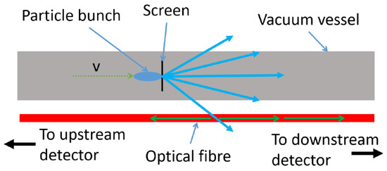
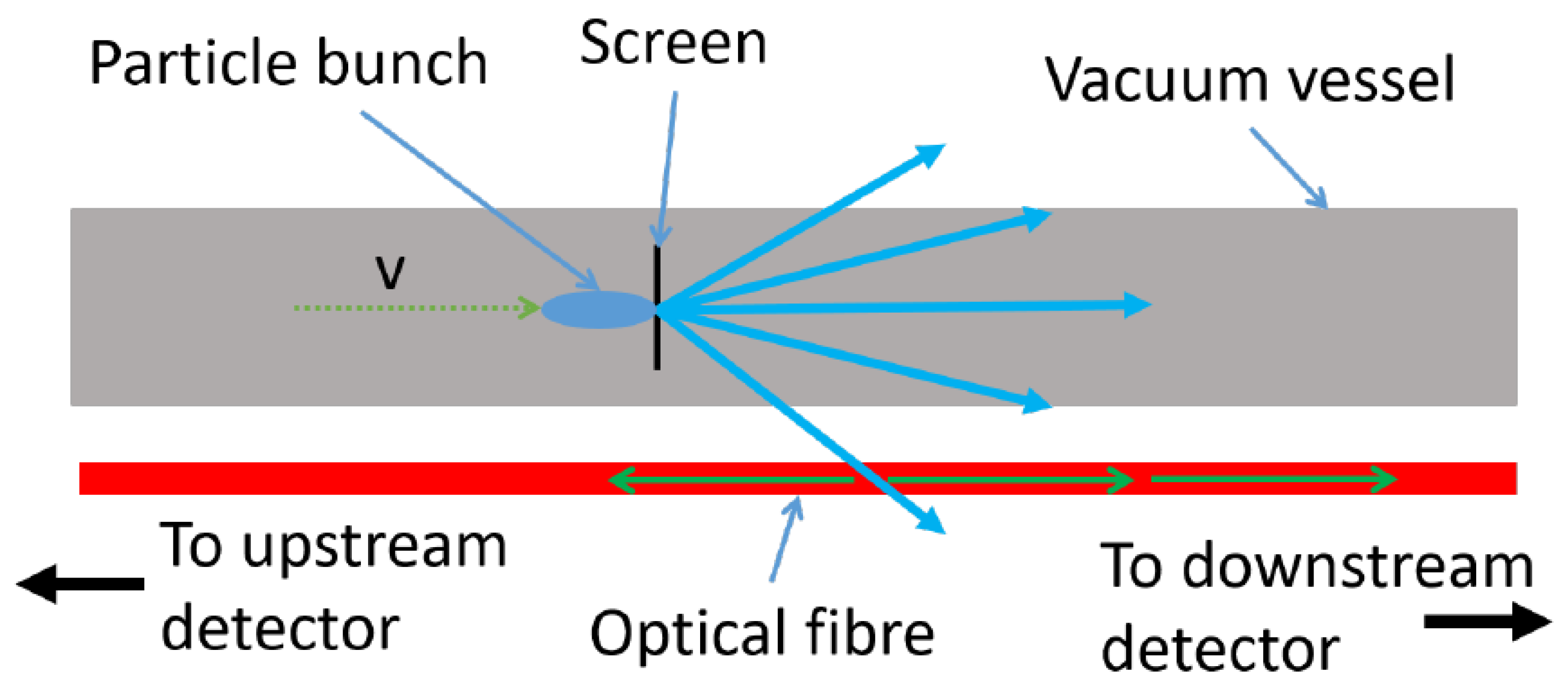
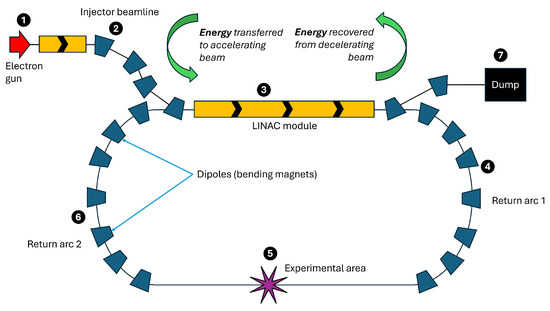
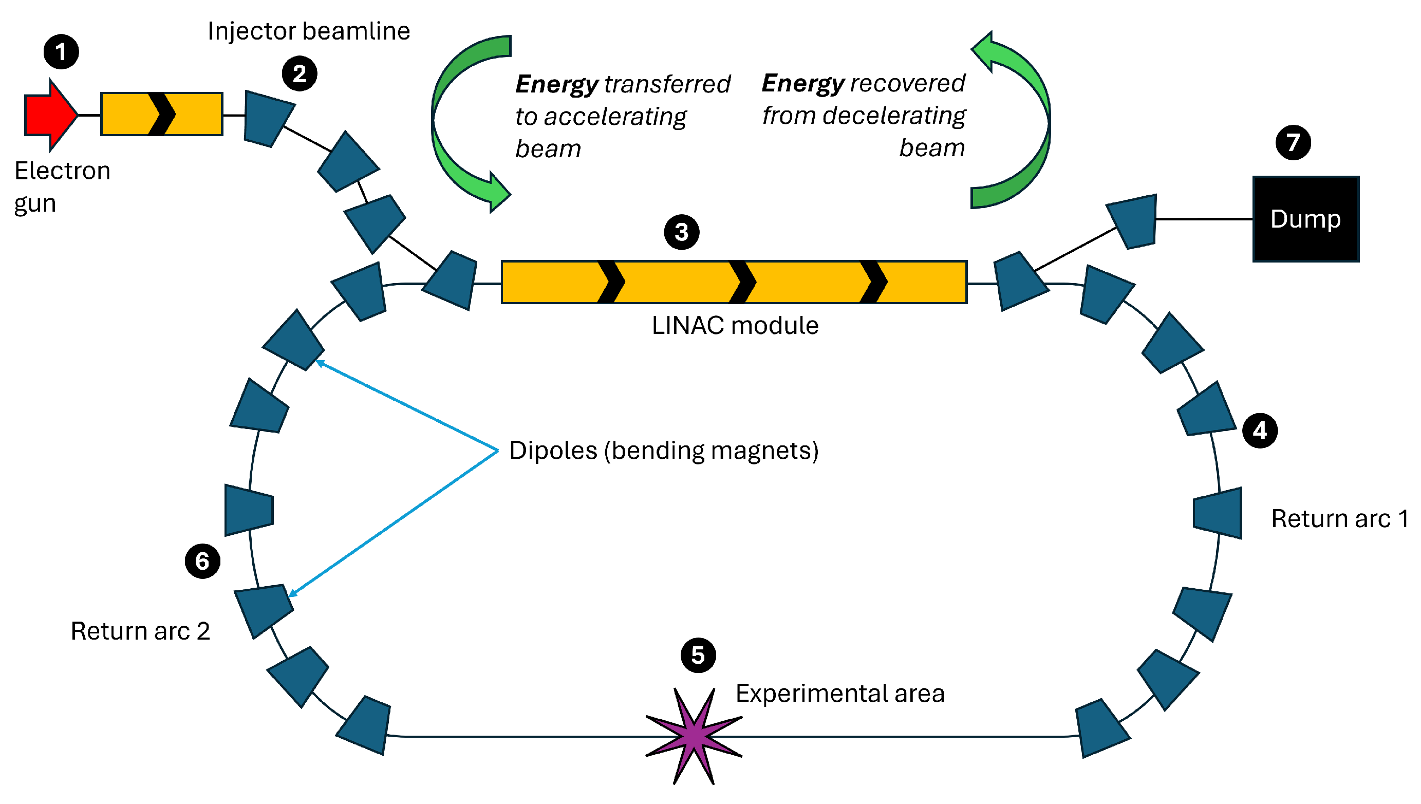
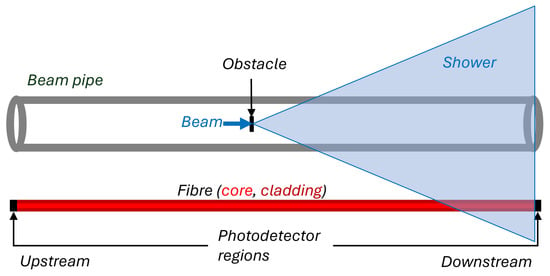
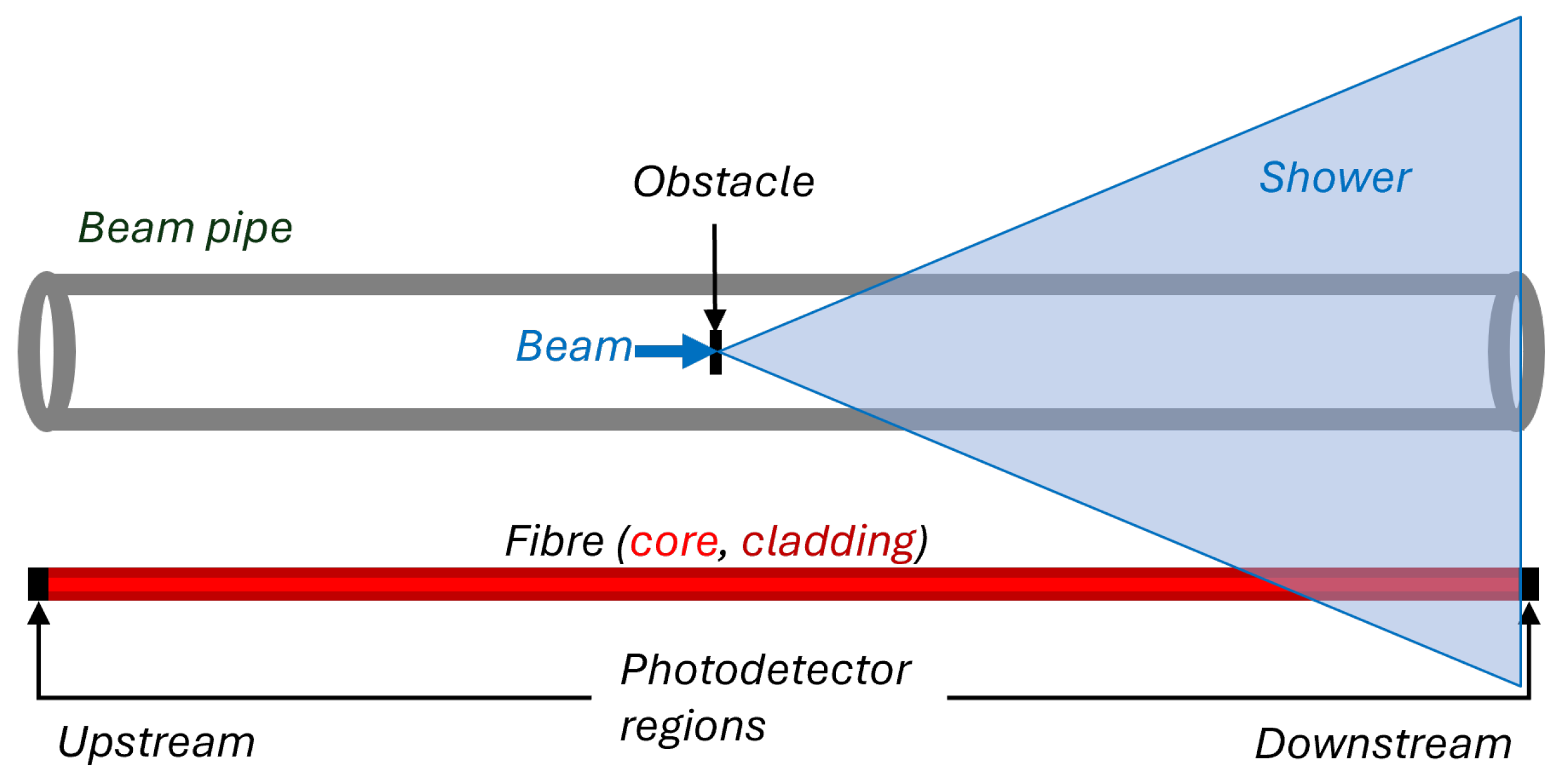
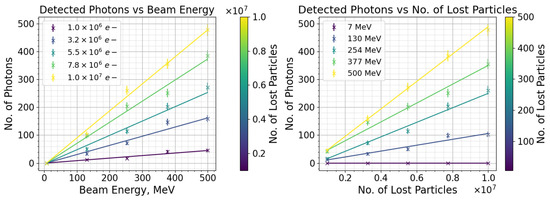
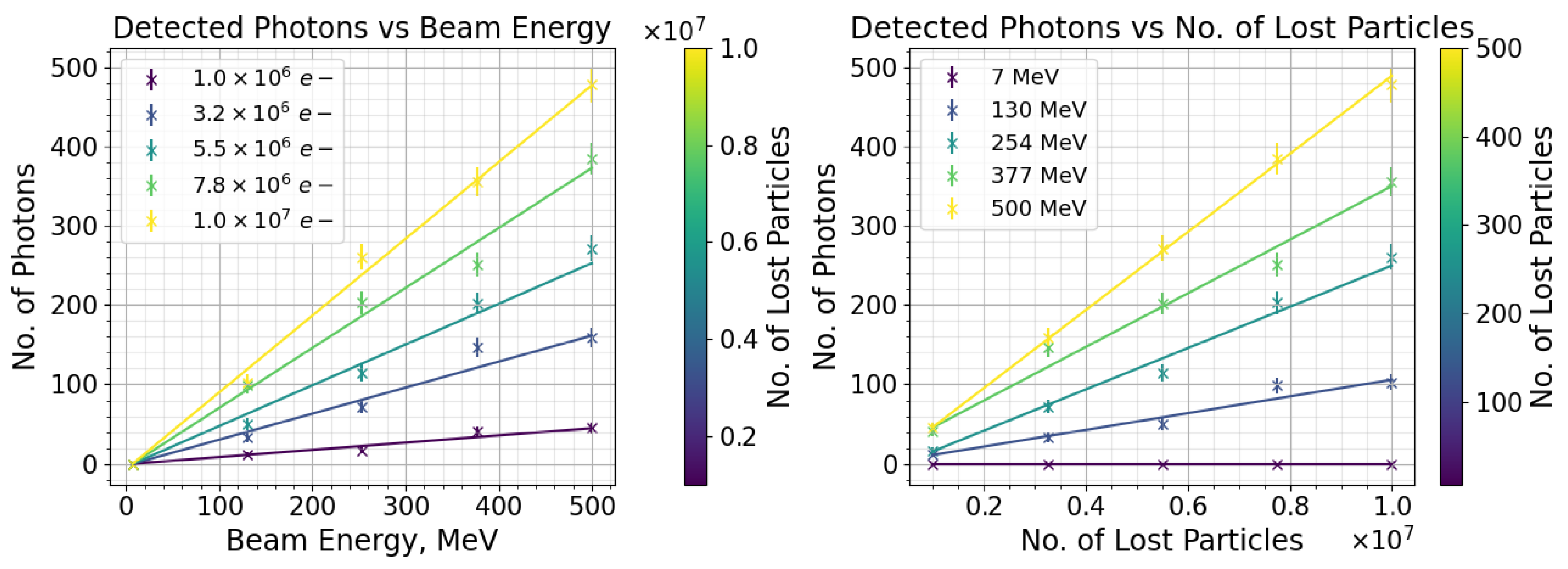
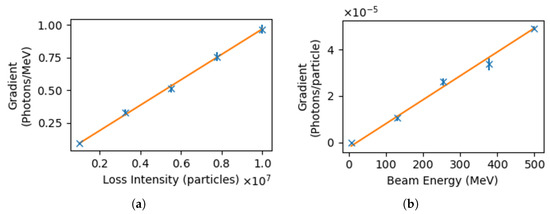
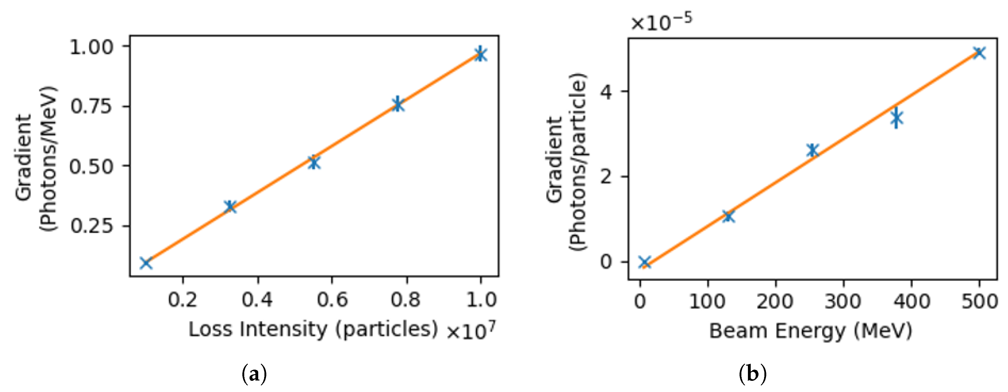
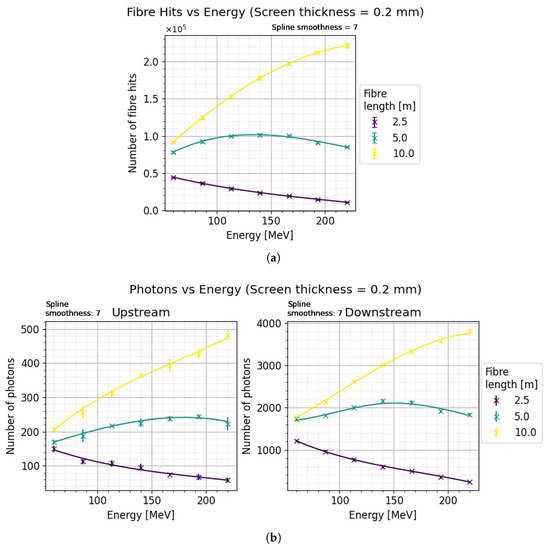
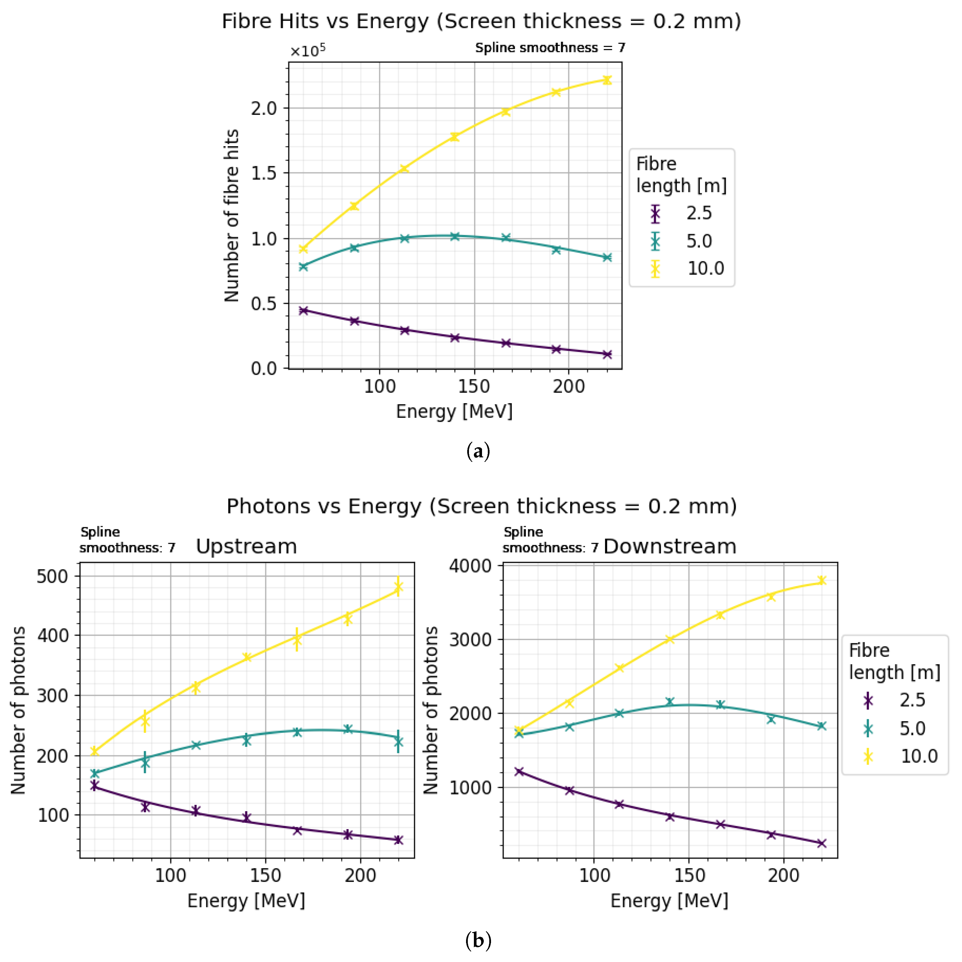
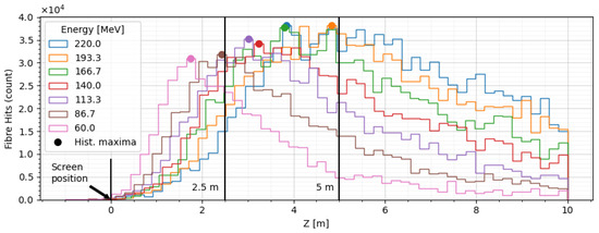
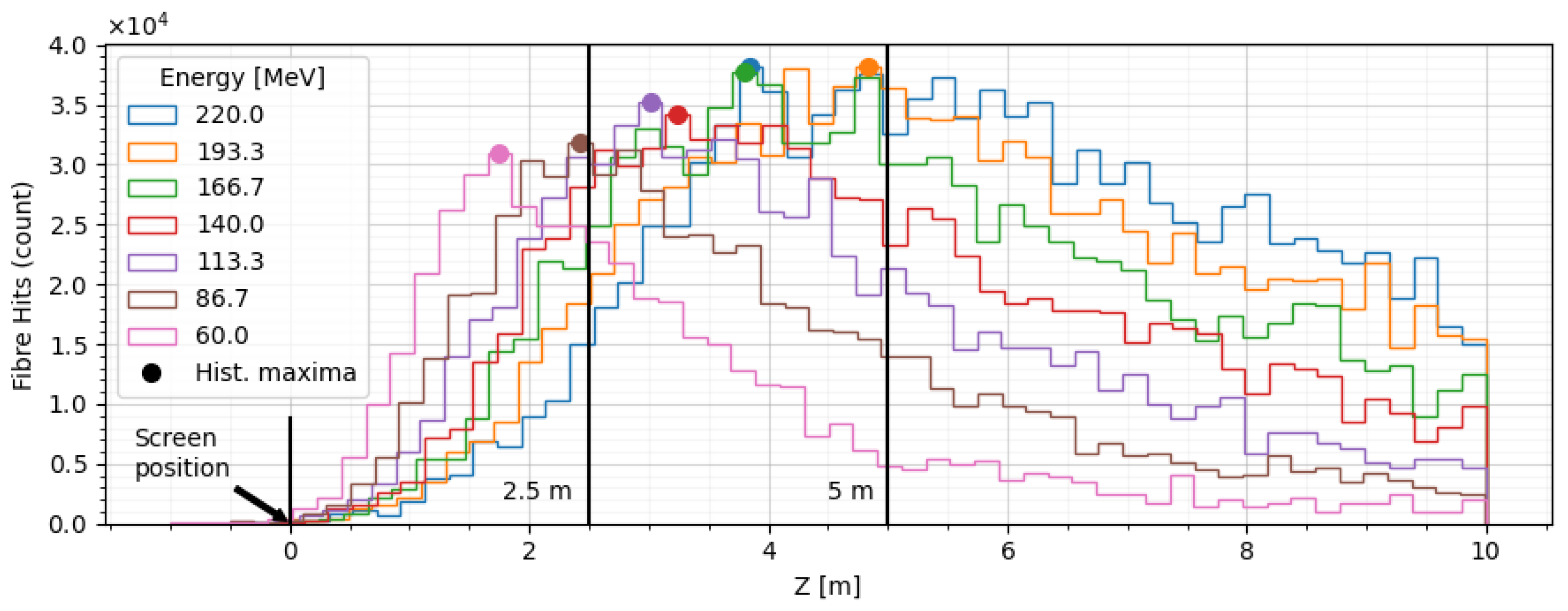
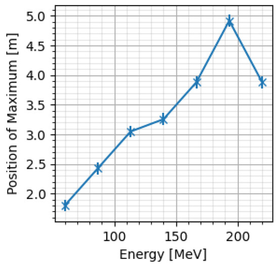
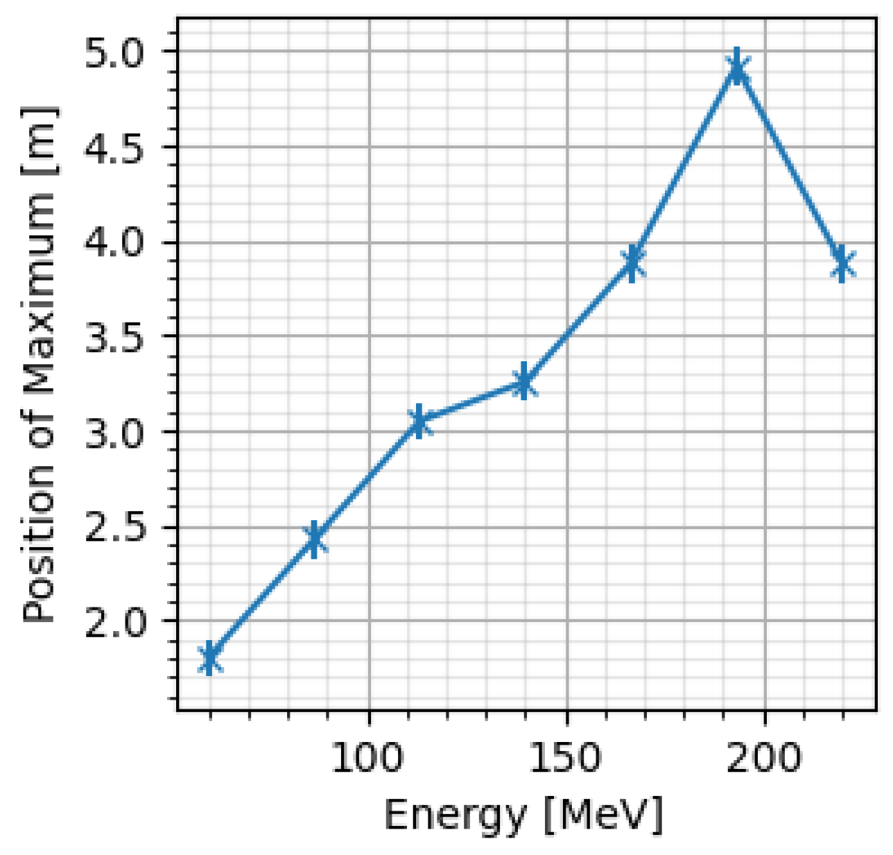
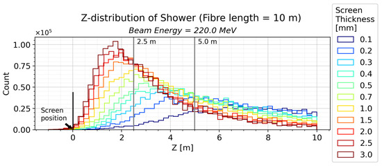
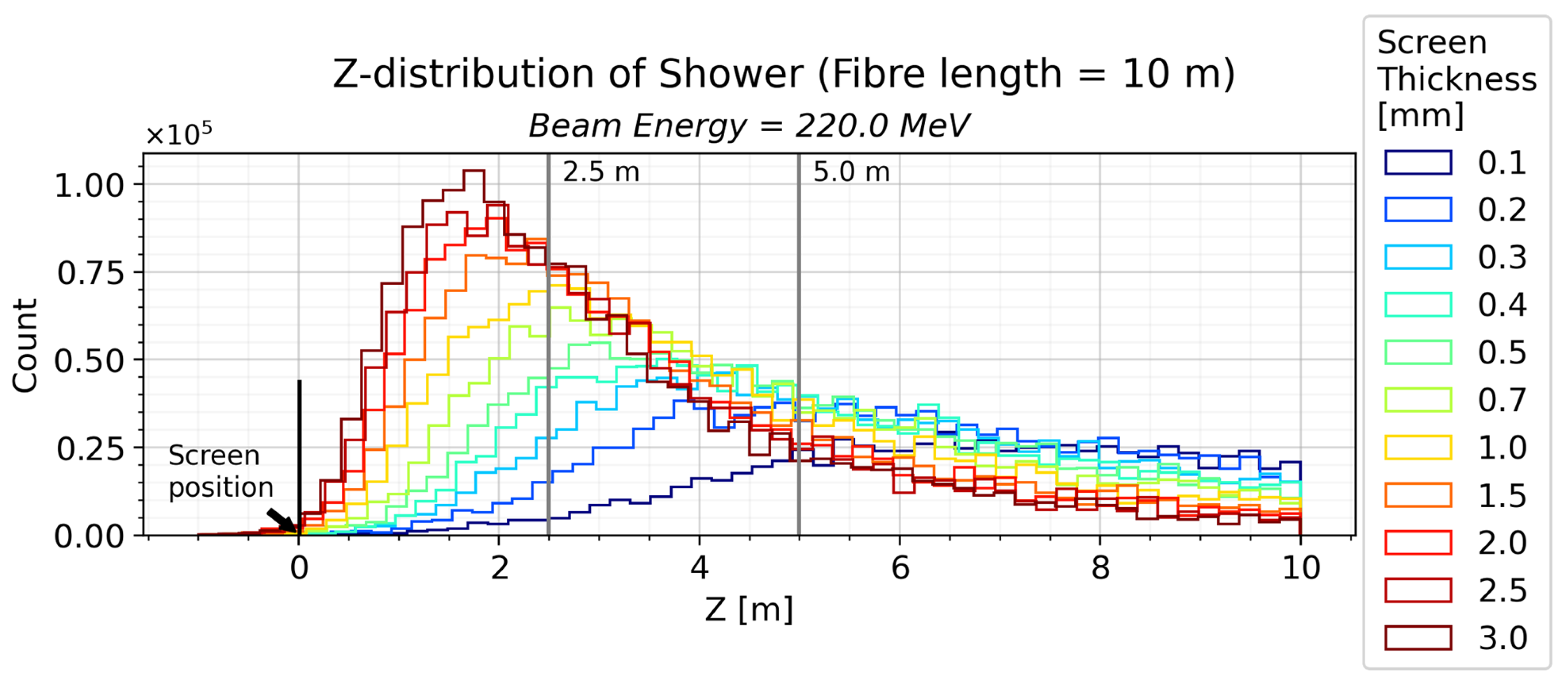
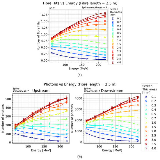
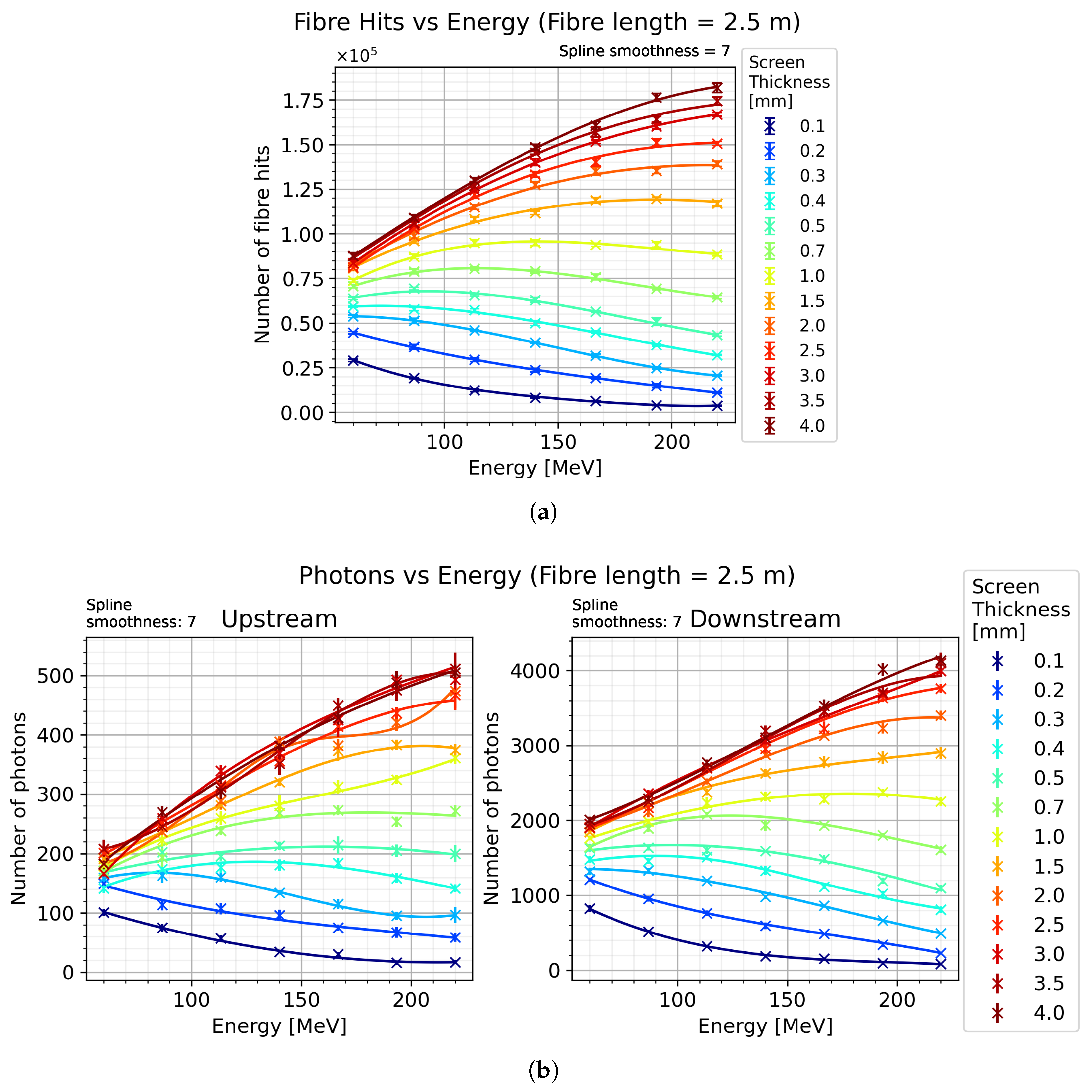
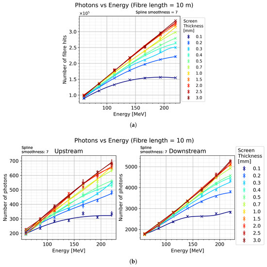
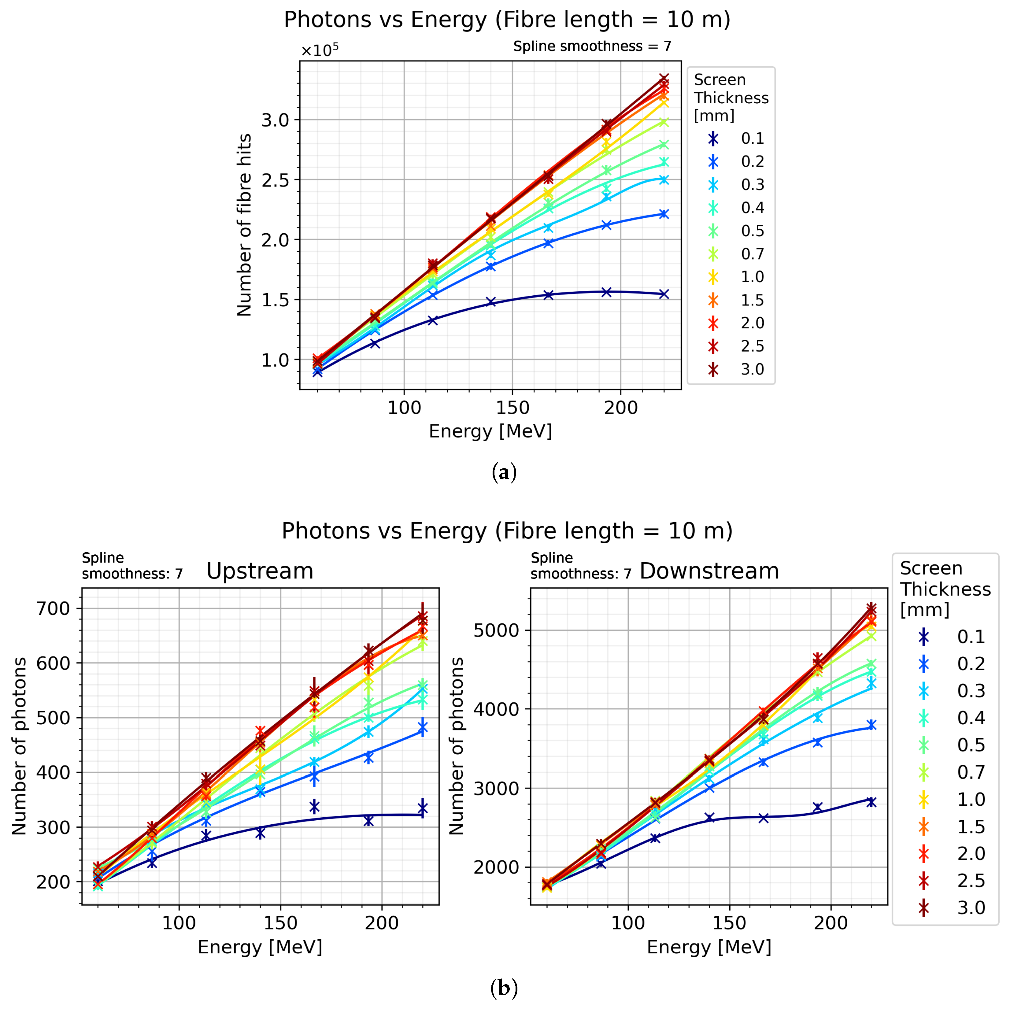
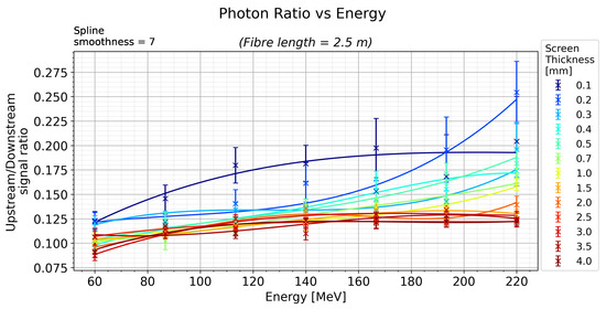
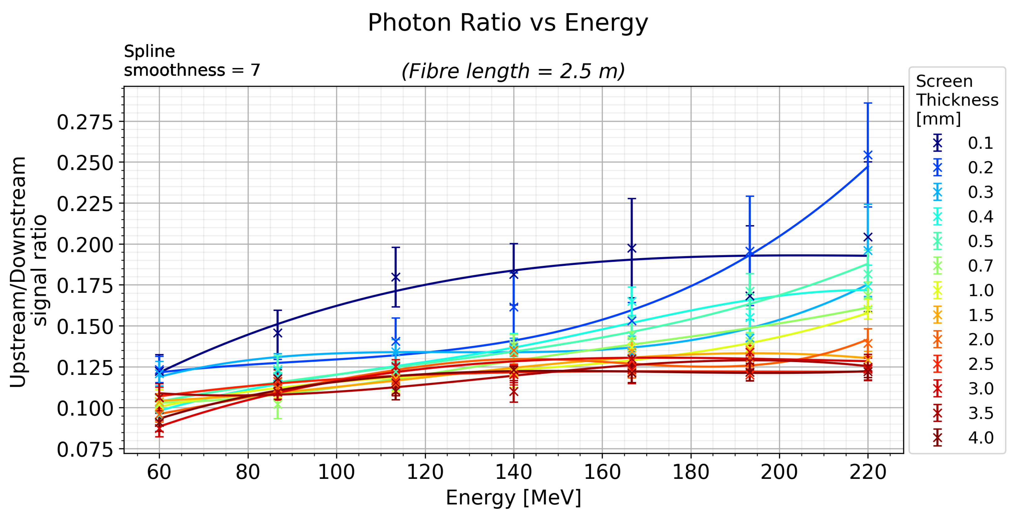
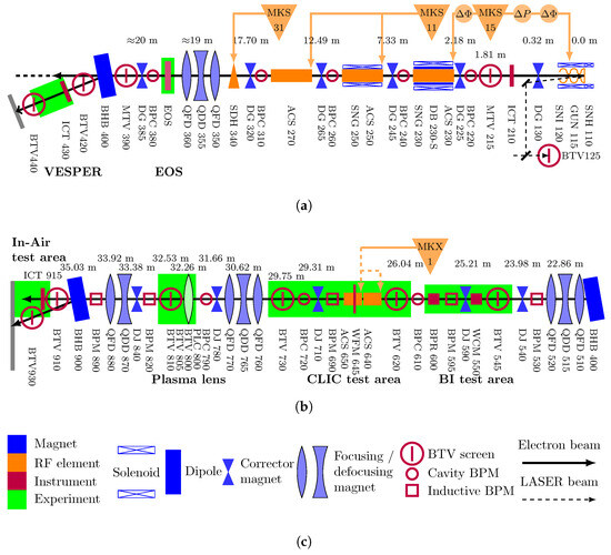
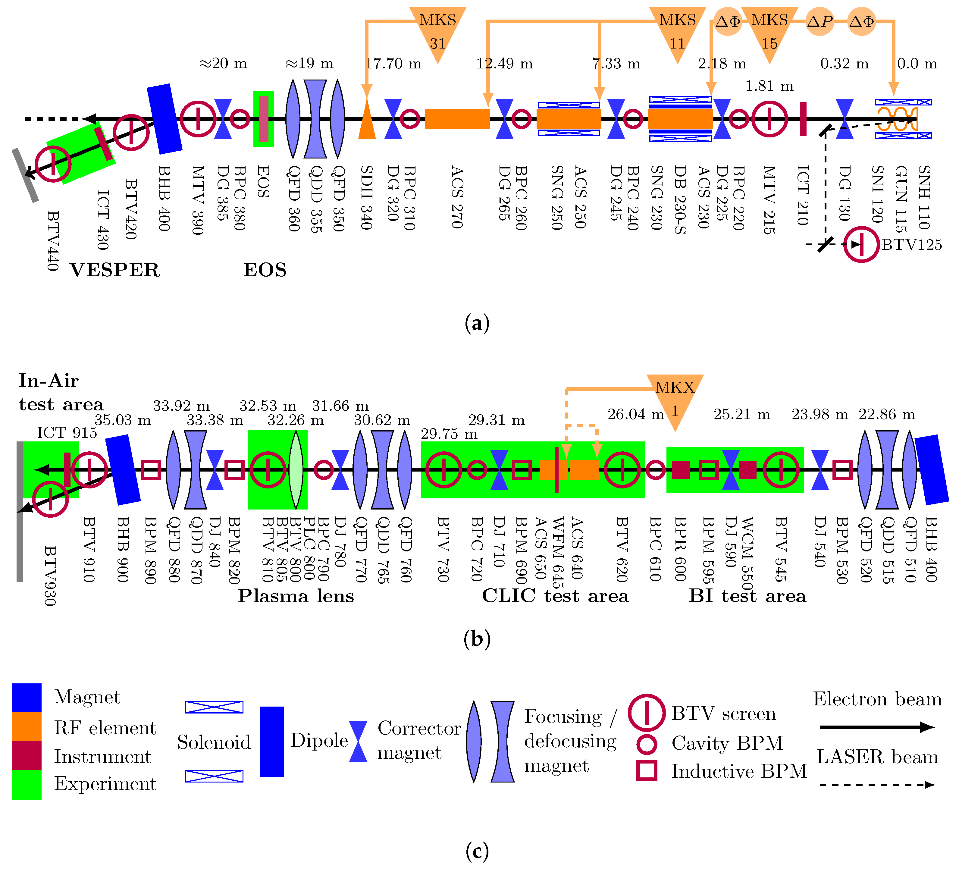
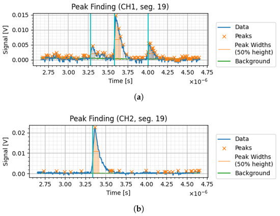
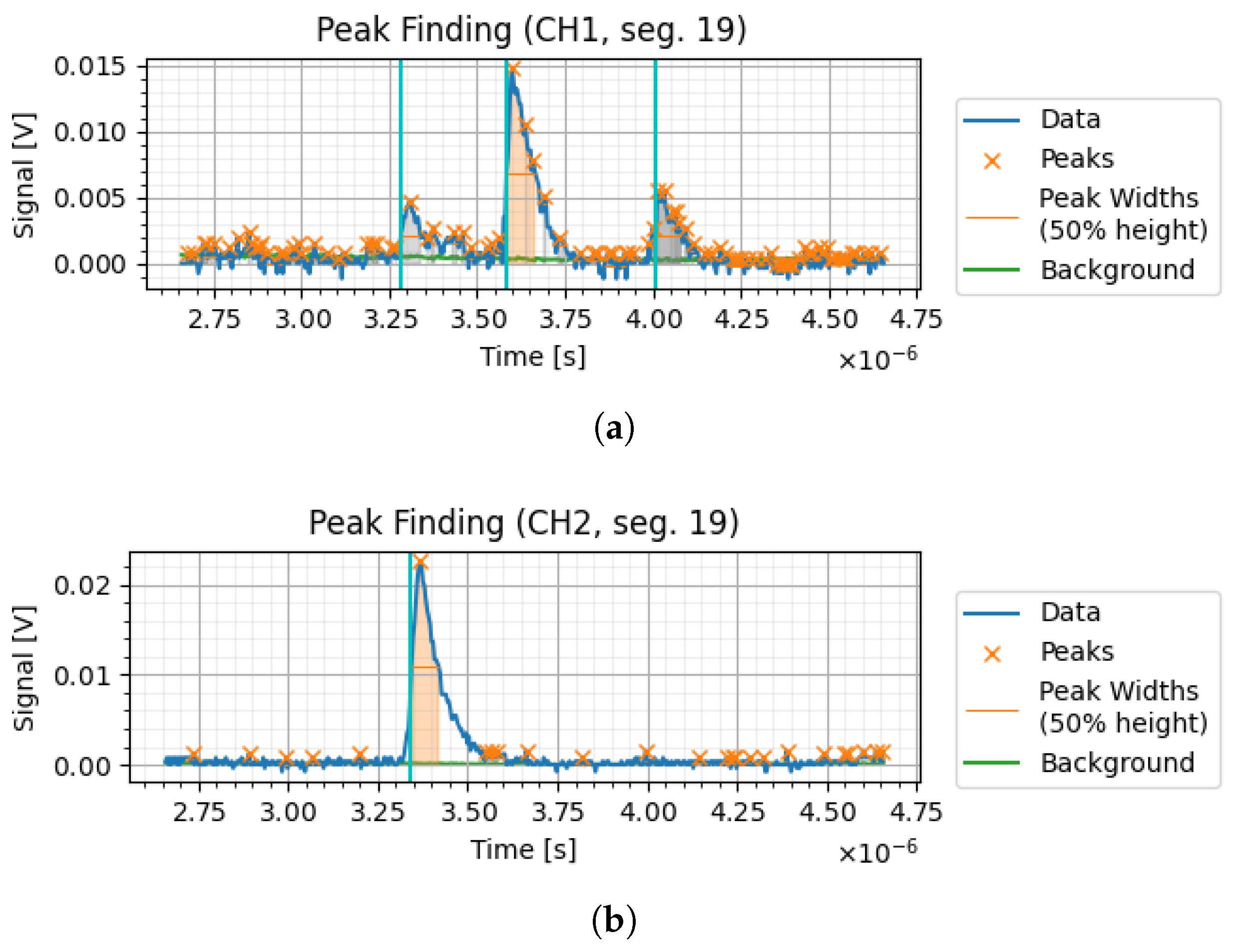
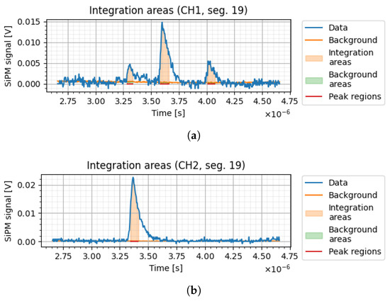
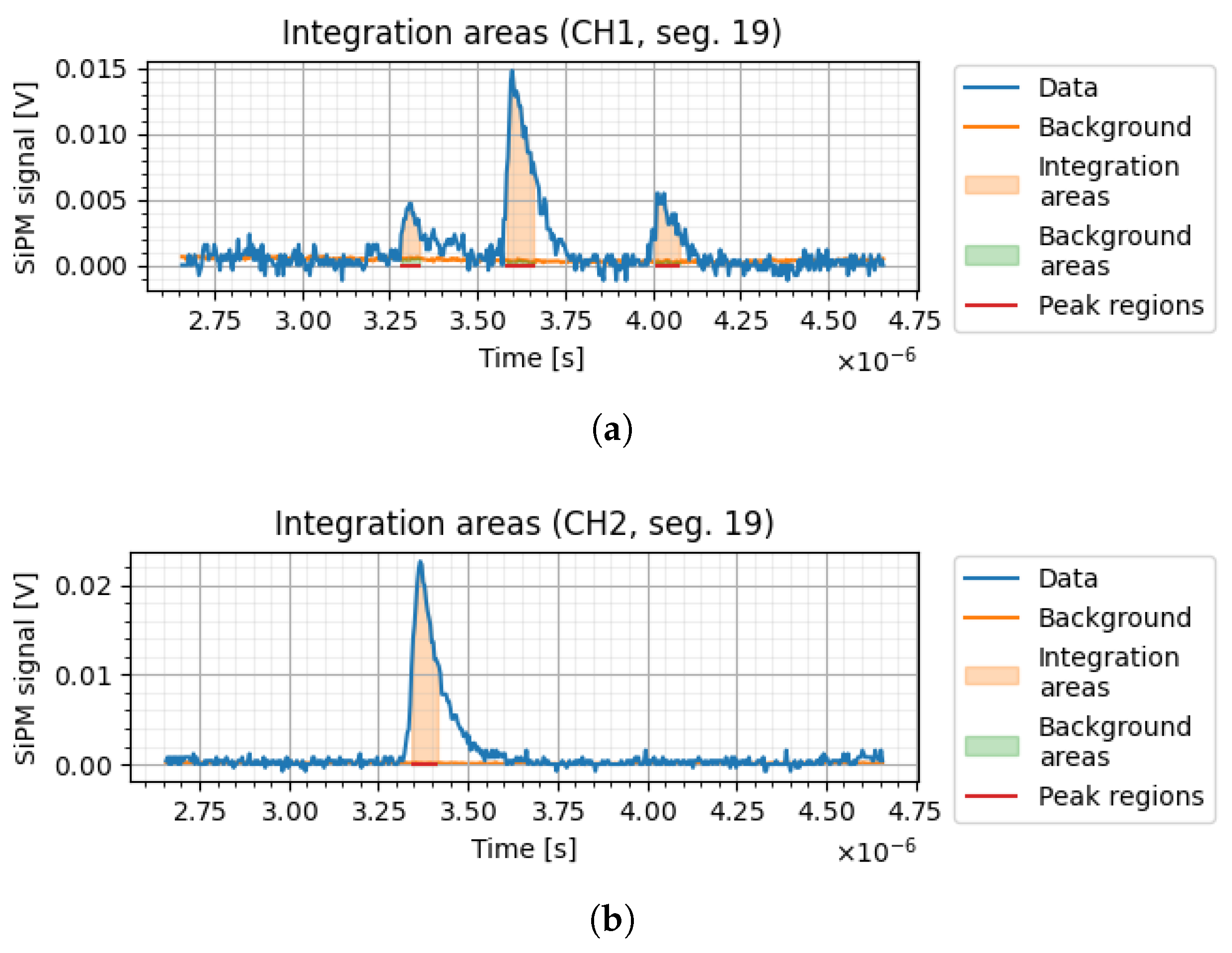
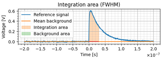
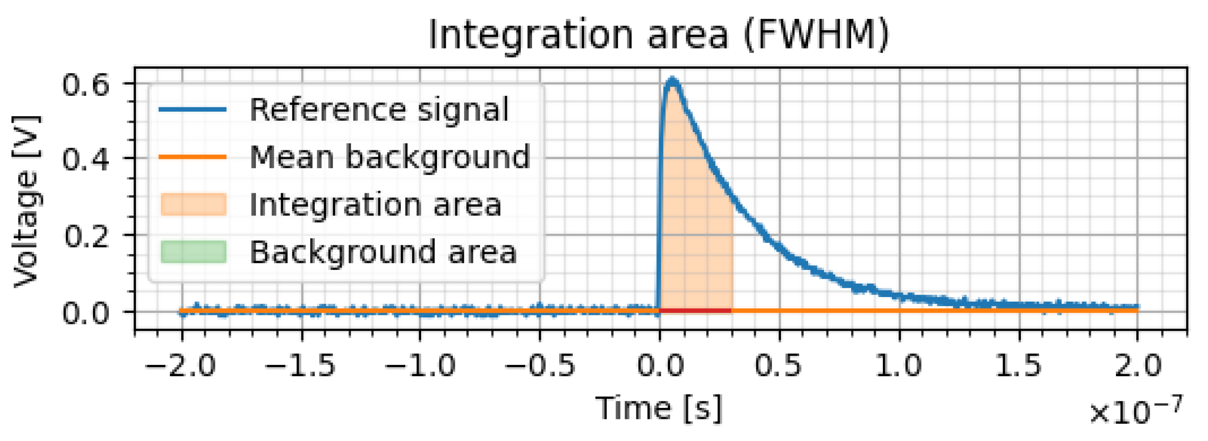
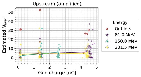
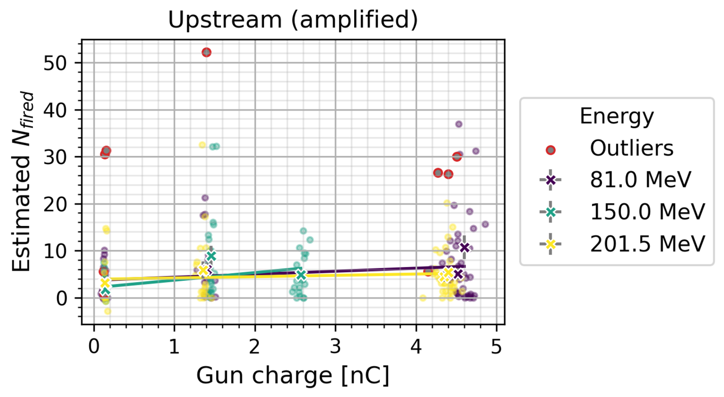
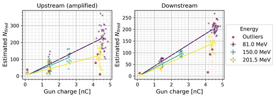
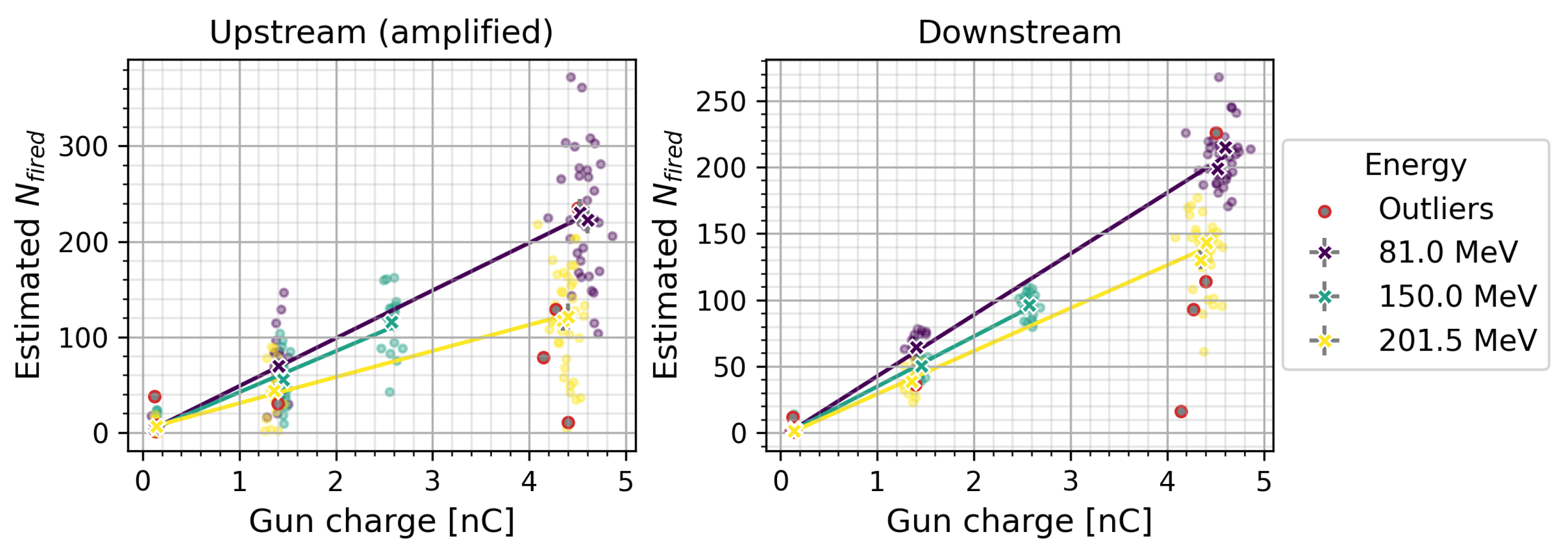
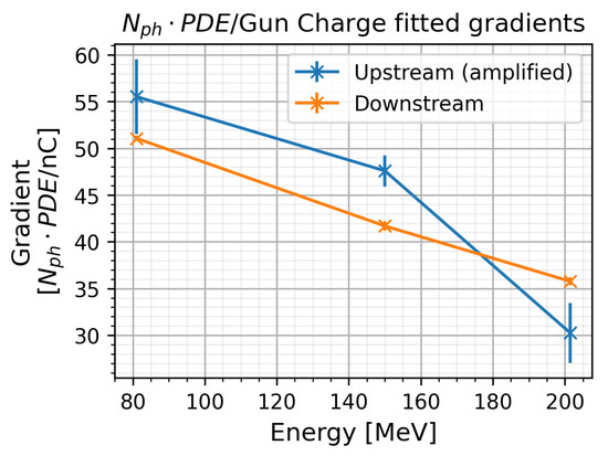
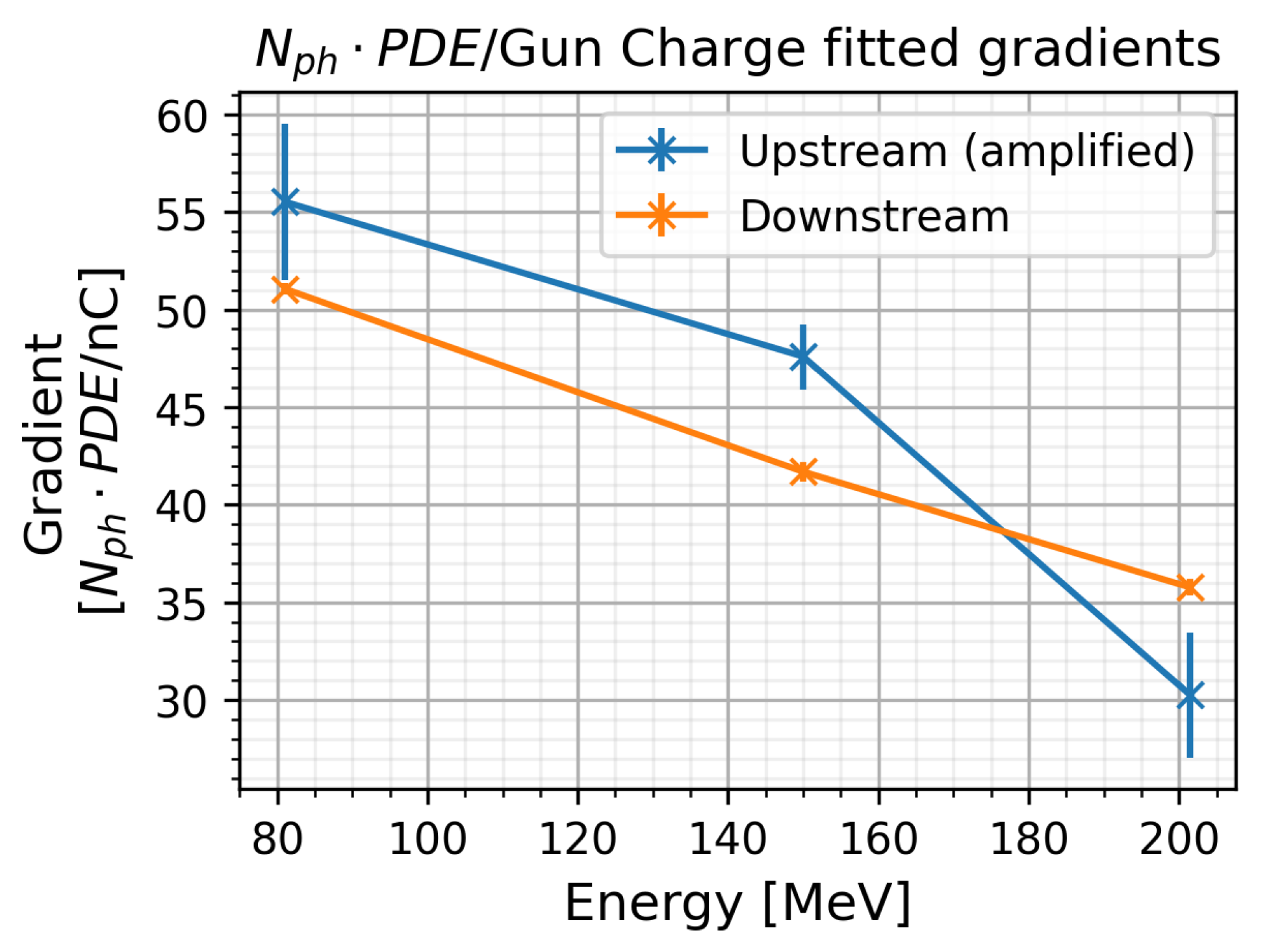
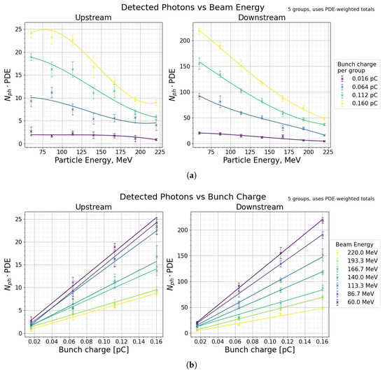
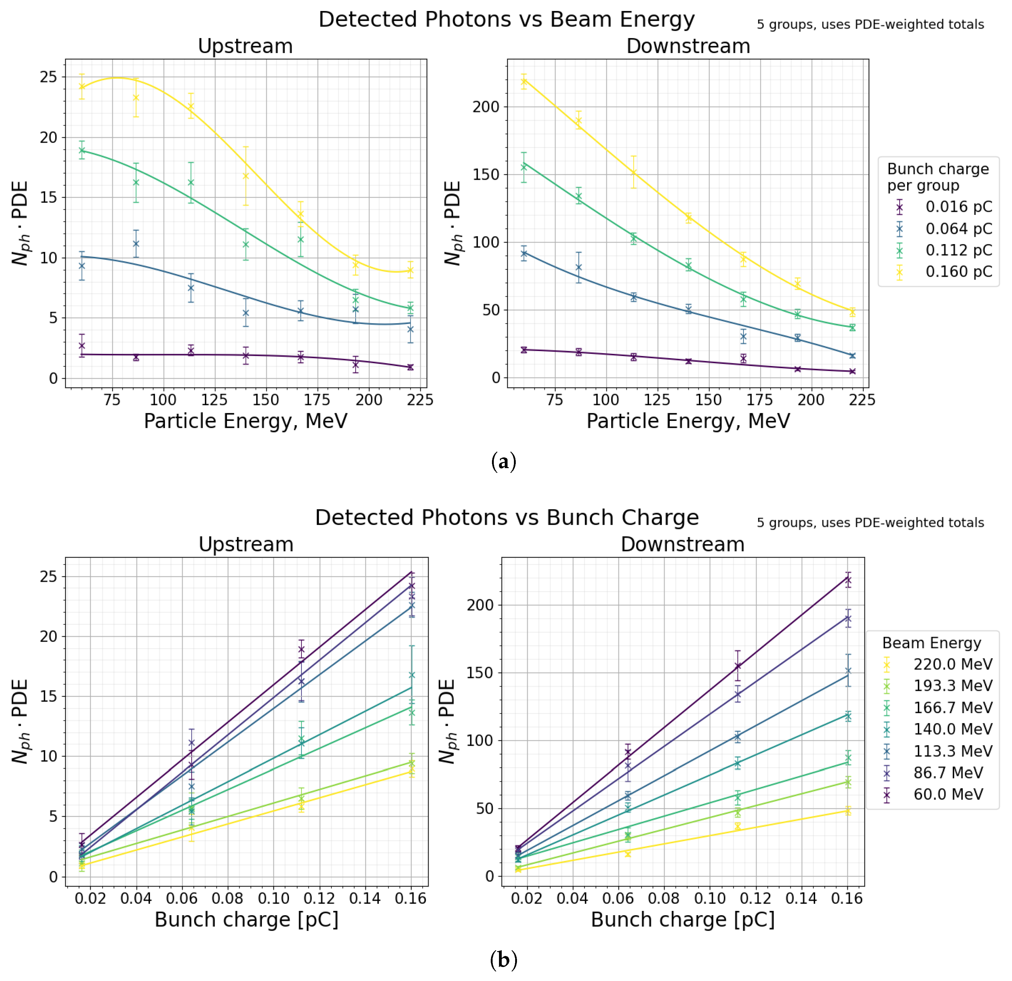
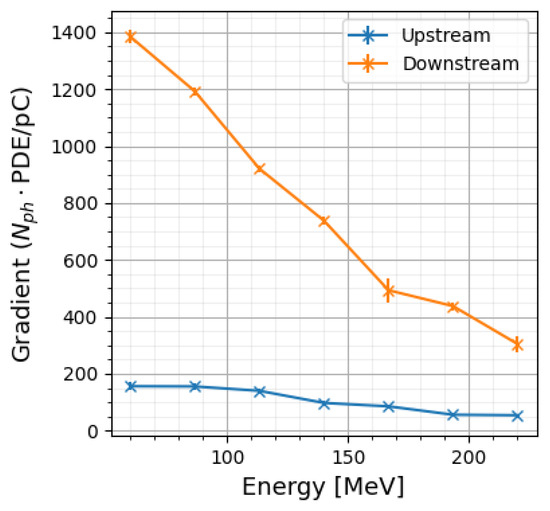
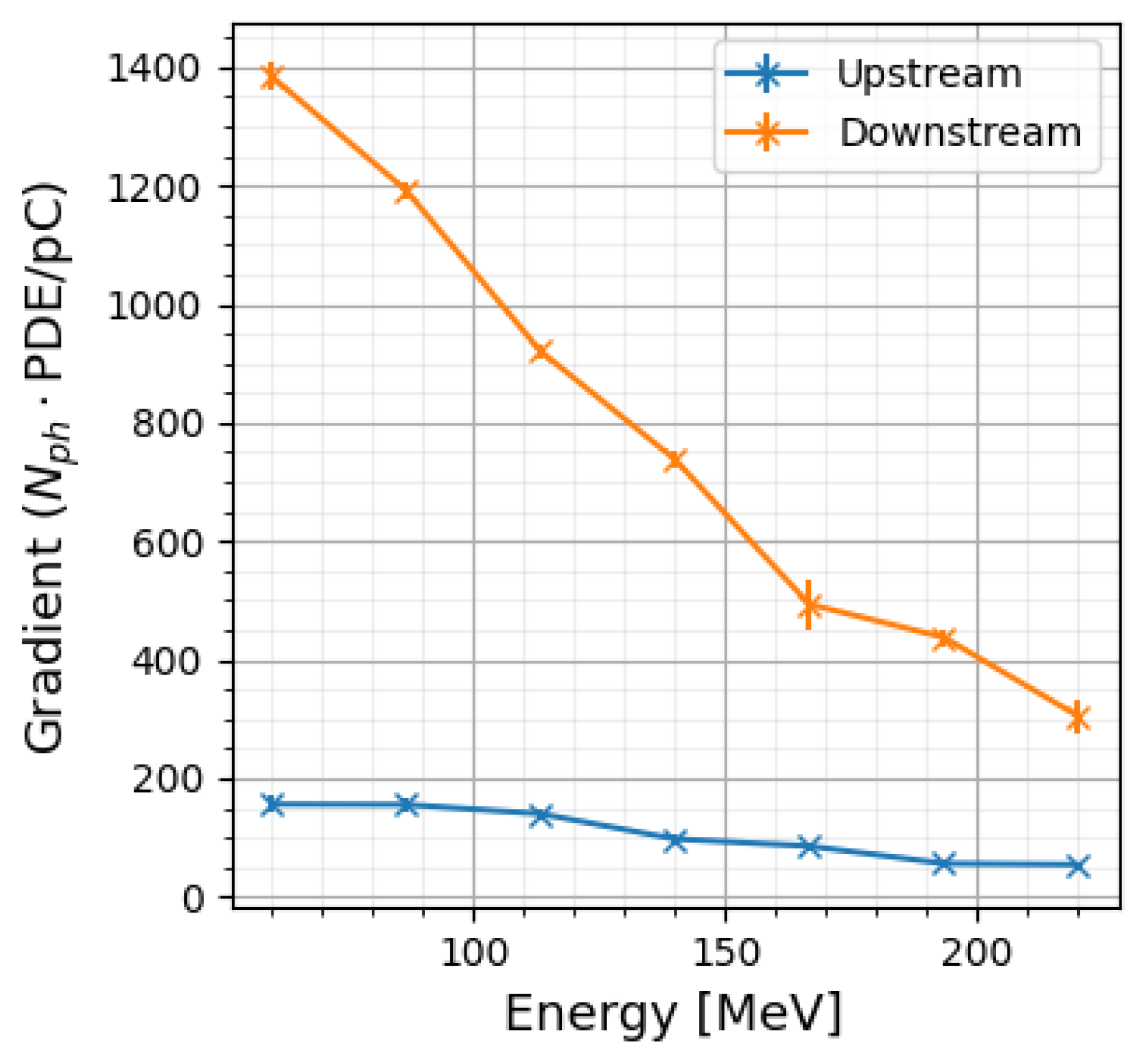

Disclaimer/Publisher’s Note: The statements, opinions and data contained in all publications are solely those of the individual author(s) and contributor(s) and not of MDPI and/or the editor(s). MDPI and/or the editor(s) disclaim responsibility for any injury to people or property resulting from any ideas, methods, instructions or products referred to in the content. |
© 2026 by the authors. Licensee MDPI, Basel, Switzerland. This article is an open access article distributed under the terms and conditions of the Creative Commons Attribution (CC BY) license.