Cross-Condition State-of-Health Estimation of Lithium-Ion Batteries via Degradation-Feature Constraints and Domain-Difference Gating

Abstract

To address the limited generalization of lithium-ion battery state-of-health (SOH) estimation under unseen aging conditions, this study proposes a degradation-feature-constrained domain-difference gated method (DFC-DGGate). Cycle-level features are constructed from capacity, voltage, local statistics, and first-order degradation variations. Three branches, namely Local ET, Trend Ridge, and Robust Huber, are used to characterize local nonlinear mapping, global degradation trends, and robust estimation, respectively. Their outputs are fused by a condition-aware domain-difference gate and further smoothed to obtain continuous SOH estimates. Cell-wise and condition-wise validations are conducted on the XJTU dataset, and external testing is performed on the NASA dataset. Under XJTU condition-wise validation, DFC-DGGate achieves an RMSE of 14.3895%, while the best-performing baseline, SVR, achieves 5.7623%. The proposed framework remains more accurate than the global Trend Ridge branch (22.3915%) but does not outperform the strongest nonlinear baselines under the substantial Sim_satellite shift. In XJTU-to-NASA validation, the anchor-corrected external extension achieves RMSEs of 20.45% and 19.10% on NASA core and NASA clean, respectively, slightly outperforming ExtraTrees on both subsets.

1. Introduction

Lithium-ion power batteries are core energy-storage components in electric vehicles, and their health status directly affects driving range, operational safety, and battery management decisions. State-of-health (SOH) is commonly used to describe the capacity or performance degradation of a battery relative to its initial state, and it is a key parameter for remaining useful life prediction, fault warning, second-life use, and maintenance management. As battery operating scenarios extend from controlled laboratory conditions to real vehicles, complex charging–discharging protocols, and multi-source data environments, SOH estimation is no longer only an accuracy problem within a single dataset. It must also cope with distribution differences among unseen cells, unseen aging conditions, and different data sources. Here, an unseen aging condition refers to an aging protocol or operating condition that is absent from the training data but appears during testing. Such conditions are important because battery degradation patterns may change with operating protocols, causing models trained on previously observed conditions to lose estimation accuracy. Therefore, improving cross-condition generalization while maintaining estimation accuracy remains an important issue in battery SOH estimation.

Data-driven methods have become an important direction for lithium-ion battery SOH estimation. Existing reviews have summarized machine-learning-based SOH estimation, battery degradation modeling, and deep-learning approaches, and have pointed out that model performance is closely related to feature quality, training data distribution, and operating-condition consistency [1,2,3]. Compared with mechanism-based models that require parameter identification, machine learning and deep learning methods can directly learn nonlinear relationships between SOH and degradation-related variables such as capacity, voltage, current, temperature, and time. End-to-end neural networks, partial-charging-data-based methods, and real-world vehicle data modeling have been used to improve the automation of SOH estimation [4,5,6]. GRU, LSTM, TCN, and CNN–Transformer structures have also been introduced for battery degradation sequence modeling and have achieved good performance on single datasets or under similar operating conditions [7,8,9,10]. However, these models often rely on strong distribution consistency between training and test data. When test samples come from new aging protocols or new experimental platforms, their prediction errors may increase.

In addition to model structure, stable degradation-feature representation is also critical for SOH estimation. Capacity-fading features directly reflect changes in battery health, voltage statistical features capture response differences caused by aging and operating conditions, and local rolling statistics and first-order variation features help describe short-term degradation trends. Incremental-capacity analysis and multi-health-factor extraction indicate that appropriate feature design can strengthen the representation of battery aging behavior [11,12]. Feng et al. [13] further compared different feature types for data-driven SOH estimation and showed that capacity, voltage, and degradation-trend features have important effects on model accuracy and stability. Nevertheless, in cross-condition tasks, relying on a single feature group or a single model structure is still insufficient to handle distribution shift. A model should capture local nonlinear relationships, preserve global degradation-trend constraints, and adapt to operating-condition differences. Recent studies on dynamic conditions, weak labels, and physics-informed degradation modeling have started to address robustness in complex scenarios [14,15,16,17]. Jiang et al. [18,19] further explored flexible parallel neural-network architectures for early battery-lifespan and RUL prediction under limited observations, demonstrating the potential of adaptive multi-branch structures for battery prognostics. However, stable extrapolation of cycle-level SOH estimation to unseen aging conditions still requires further improvement.

Overall, existing SOH estimation methods have made substantial progress, but stable estimation under unseen aging conditions remains challenging. Existing transfer and domain-adaptation methods mainly improve cross-domain representation or parameter transfer, whereas it remains difficult to simultaneously preserve local nonlinear fitting, global degradation trends, and robustness to condition shifts. To reduce performance degradation caused by distribution shift, transfer learning and domain adaptation have been introduced into battery SOH estimation. Chen et al. [20] investigated transfer learning strategies under domain shift and showed that differences between data domains directly affect capacity estimation. Dou et al. [21] improved cross-domain SOH estimation through latent-space consistency, while Zhu et al. [22] adopted a Domain-Adaptive Transformer for cross-domain SOH and RUL estimation. To address this gap, this paper proposes DFC-DGGate, which differs from existing single-model or representation-transfer approaches by combining local nonlinear, global trend, and robust estimation branches through condition-aware gating, followed by lightweight smoothing for stable cross-condition SOH estimation. Ensemble learning and physics-informed machine learning have also been explored to improve SOH estimation robustness under various operating conditions [23,24]. The method uses cycle-level degradation features as inputs and constructs three branches, namely a local tree-model branch, a degradation-trend branch, and a robust linear branch, to characterize local nonlinear mapping, global degradation trends, and robustness against abnormal fluctuations. A domain-difference gate is then introduced to perform condition-aware fusion of the branch outputs, followed by a smoothing module to improve the continuity of SOH prediction sequences. The XJTU battery dataset [25], consisting of 18650 NCM cells (LiNi_0.5Co_0.2Mn_0.3O₂), is used as the main modeling dataset for cell-wise and condition-wise validation. The NASA dataset [26], for which the original repository does not specify the exact electrode chemistry, is further used for external validation.

The main contributions and novelties of this work are summarized as follows:

A cycle-level degradation-feature system covering capacity and energy, voltage statistics, local statistics, and first-order variations is constructed for SOH estimation under unseen aging conditions.

A DFC-DGGate framework is proposed to integrate Local ET, Robust Huber, and Trend Ridge through condition-aware domain-difference gating and lightweight smoothing.

A multi-level validation protocol covering unseen cells, unseen aging conditions, and XJTU-to-NASA transfer is established to evaluate cross-condition performance and cross-dataset transfer limitations.

The remainder of this paper is organized as follows. Section 2 presents the proposed methodology; Section 3 describes the datasets and experimental settings; Section 4 reports and analyzes the results; Section 5 discusses the main findings and limitations; and Section 6 concludes the study.

2. Methods

2.1. Research Workflow

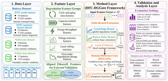
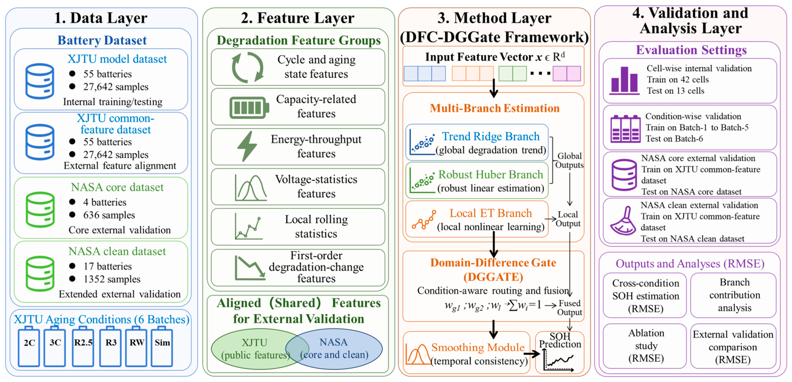
The overall workflow of this study is shown in Figure 1, including the data, feature, method, and validation-analysis layers. In the data layer, two datasets are constructed from the same 55 XJTU cells and 27,642 cycle-level samples in the XJTU dataset [25] for different purposes. The XJTU modeling dataset uses XJTU-specific degradation features for internal modeling and cross-condition validation, whereas the XJTU common-feature dataset uses a separately constructed feature space aligned with the NASA dataset [26] for XJTU-to-NASA external validation. In this study, NASA core refers to the four commonly used cells B0005, B0006, B0007, and B0018, whereas NASA clean refers to the 17-cell subset retained after screening for data-field completeness, capacity-record continuity, and a reasonable SOH range. The XJTU dataset covers six aging conditions, including 2C, 3C, R2.5, R3, RW, and Sim_satellite. Here, R2.5 and R3 denote variable-rate discharge protocols with cutoff voltages of 2.5 and 3.0 V, respectively, while RW denotes a random-walk discharge protocol with randomized discharge current and duration.

Figure 1. Overall research workflow. The XJTU modeling dataset is used for internal and cross-condition validation, whereas the XJTU common-feature dataset uses NASA-aligned features for external validation.

In the feature layer, cycle-level degradation features are constructed from cycle state, capacity and energy variation, voltage statistics, local rolling statistics, and first-order degradation changes. Capacity and energy features reflect battery performance degradation, voltage statistics provide additional information on operating-condition-dependent voltage responses, and rolling statistics and first-order variations describe short-term fluctuations and local degradation rates. For XJTU-to-NASA external validation, only alignable variables related to voltage, current/load, temperature, cycle, and time are retained to form a common feature space, reducing the influence of inconsistent data fields across datasets.

In the method layer, the DFC-DGGate estimation framework is developed. It consists of three branches: Trend Ridge, Robust Huber, and Local ET, which are used to characterize the global degradation trend, improve robustness to abnormal fluctuations, and capture local nonlinear mapping relationships, respectively. A domain-difference gate then performs condition-aware fusion of the branch outputs according to whether the aging condition is represented in the training domain. Finally, a smoothing module is applied to constrain abrupt prediction fluctuations across consecutive cycles and obtain the final SOH estimates.

In the validation-analysis layer, three tasks are designed: cell-wise internal validation, condition-wise cross-condition validation, and NASA external validation. Cell-wise validation evaluates generalization to unseen cells. Condition-wise validation uses XJTU Batch-1 to Batch-5 for training and Batch-6 for testing, assessing the model’s adaptability to an unseen aging condition. NASA core and NASA clean are used to examine cross-dataset transfer performance. The proposed DFC-DGGate method is evaluated in terms of SOH estimation error, branch contribution, ablation results, and external validation performance.

2.2. Structure of the DFC

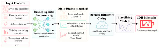
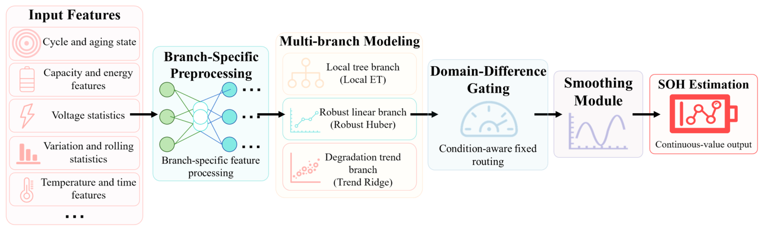
The structure of the DFC-DGGate model is shown in Figure 2. The model takes cycle-level degradation features as inputs, including cycle and aging-state features, capacity and energy features, voltage statistical features, local rolling statistical features, first-order degradation variation features, and auxiliary variables such as temperature and time. Missing values are imputed using training-set statistics. Feature standardization is applied to the Trend Ridge and Robust Huber branches, whereas Local ET uses the same numerical features without scale transformation because tree-based partitioning is insensitive to feature scaling. In this study, the degradation-feature constraint is reflected in two aspects: degradation-related cycle-level features are introduced at the input side, and the trend branch together with the smoothing module is used at the output side to reduce non-physical fluctuations in SOH prediction sequences.

Figure 2. Structure of the DFC-DGGate model.

DFC-DGGate contains three estimation branches: Trend Ridge, Robust Huber, and Local ET, which are built on ridge regression, Robust Huber estimation, and extremely randomized trees, respectively [27,28,29]. The Trend Ridge branch describes the overall degradation trend of SOH with cycle progression. The Robust Huber branch reduces the influence of abnormal fluctuations and local noise. The Local ET branch learns local nonlinear mappings and is suitable for capturing detailed variations under similar conditions and degradation stages. These branches provide complementary SOH predictions from the perspectives of local fitting, robust estimation, and trend constraint, preventing the model from relying on a single estimator or a single feature relationship.

The domain-difference gate is implemented as a lightweight condition-aware routing mechanism rather than a learnable neural gating network. In this study, domain difference specifically refers to whether an aging condition is represented in the training-domain condition set; it is therefore a condition-level indicator rather than a continuous measure of covariate shift, label shift, or representation discrepancy. The three branch outputs are fused according to this indicator, and the complete weight calculation and calibration procedure are given in Section 2.3.

After gate fusion, a smoothing module is introduced to constrain SOH predictions over consecutive cycles. Since battery SOH degradation is generally continuous, individual cycle-level predictions should not exhibit abrupt jumps. Smoothing reduces the influence of local abnormal prediction points and makes the estimated SOH trajectory more consistent with battery degradation behavior. This smoothing operation is applied only within the consecutive cycle sequence of the same cell, rather than across different cells or datasets.

Overall, DFC-DGGate is not a simple average of multiple models. It integrates degradation-feature constraints, multi-branch estimation, domain-difference gating, and smoothed output. By combining local nonlinear fitting with trend and robustness constraints, the model aims to improve SOH estimation generalization under unseen aging conditions.

2.3. Model Training and Evaluation Metrics

This study uses cycle-level samples as modeling units. For the i-th cycle sample, the input feature vector is defined as

$$x_i=[x_{i1},x_{i2},\cdots ,x_{id}]\in {\mathbb{R}}^d$$

(1)

where $d$ is the feature dimension. The input features include cycle-state, capacity, energy, voltage-statistical, local rolling-statistical, and first-order degradation-variation variables. The model output is the SOH estimate of the corresponding cycle. In this study, SOH is defined by the capacity retention ratio:

$$y_i={\displaystyle \frac{Q_i}{Q_0}}\times 100\%$$

(2)

where $Q_i$ denotes the degradation-capacity value of the i-th cycle, and $Q_0$ is the first valid value of the corresponding degradation-capacity trajectory. For protocols containing partial-discharge cycles, the degradation-capacity trajectory is reconstructed from capacity-test cycles using cubic interpolation, with linear interpolation used as a fallback; otherwise, the measured discharge capacity is used directly. Samples with SOH values above 100% are retained without truncation or removal. Such values represent capacity retention relative to the reconstructed initial reference and may arise from capacity activation, reference-capacity differences, or interpolation/extrapolation of sparse capacity-test points. This treatment avoids artificial bias introduced by clipping.

For the Trend Ridge and Robust Huber branches, the input features are standardized using training-set statistics as

$$x_{ij}^{*}={\displaystyle \frac{x_{ij}-{\mu }_j}{{\sigma }_j}}$$

(3)

where ${\mu }_j$ and ${\sigma }_j$ are the mean and standard deviation of the j-th feature in the training set, respectively, and $x_{ij}^{*}$ is the standardized feature. Missing-value imputation and, where required, standardization parameters are calculated only from the training set and then applied unchanged to the corresponding test or external validation set to avoid data leakage. In the XJTU-to-NASA external validation, these parameters are calculated from the XJTU common-feature training set without using any statistical information from the NASA test data.

DFC-DGGate adopts a multi-branch estimation structure. For input xi and its standardized form $x_i^{*}$, the Local ET, Robust Huber, and Trend Ridge branches output three SOH estimates:

$${\widehat{y}}_i^L=f_L(x_i),\hspace{1em}{\widehat{y}}_i^R=f_R(x_i),\hspace{1em}{\widehat{y}}_i^T=f_T(x_i)$$

(4)

where ${\widehat{y}}_i^L$, ${\widehat{y}}_i^R$, and ${\widehat{y}}_i^T$ denote the outputs of the Local ET, Robust Huber, and Trend Ridge branches, respectively. The Local ET branch mainly learns local nonlinear relationships, the Robust Huber branch reduces the influence of abnormal fluctuations and local noise, and the Trend Ridge branch represents the overall SOH degradation trend with cycle progression.

To account for differences among aging conditions, a domain-difference gate is introduced to assign condition-level routing weights to the three branch outputs. The gate-weight vector is expressed as

$$w_i=[w_i^L,w_i^R,w_i^T]$$

(5)

with the following constraints:

$$w_i^L+w_i^R+w_i^T=1,\hspace{1em}{w}_i^L,w_i^R,w_i^T\ge 0$$

(6)

where $w_i^L$, $w_i^R$, and $w_i^T$ denote the weights of Local ET, Robust Huber, and Trend Ridge, respectively. Let $c_i$ denote the aging condition of sample i, and let ${\mathcal{C}}_{tr}$ denote the set of aging conditions represented in the training data. The condition-level domain indicator is defined as

$$d_i=\left\{\begin{array}{ll}0,\hfill & c_i\in {\mathcal{C}}_{train}\hfill \\ 1,\hfill & c_i\notin {\mathcal{C}}_{train}\hfill \end{array}\right.$$

(7)

The gate-weight vector is then calculated as

$$w_i=(1-d_i)w^{seen}+d_i{w}^{unseen}$$

(8)

For the given conditions, $w^{seen}=[0.88,0.02,0.10]$, where the components correspond to Local ET, Robust Huber, and Trend Ridge, respectively.

$$w^{unseen}=\underset{w\in \Delta }{\arg \min }{\displaystyle \frac{1}{K}}{\displaystyle {\displaystyle \sum _{k=1}^K}{\mathrm{RMSE}}_k}(w)$$

(9)

where K = 5 and Δ denotes the non-negative simplex defined by Equation (6). The LOCO calibration gives $w^{unseen}=[0.50,0.00,0.50]$, corresponding to Local ET, Robust Huber, and Trend Ridge, respectively. Batch-6 is not used during weight calibration.

The three regression branches are trained first, after which the gate weights are calibrated and fixed; therefore, DFC-DGGate adopts a staged training procedure rather than end-to-end joint optimization. In the cell-wise setting, conditions represented in the training set use wseen, whereas the unseen Batch-6 Sim_satellite condition in condition-wise testing uses the LOCO-calibrated wunseen.

The gated SOH prediction is then obtained by

$${\widehat{y}}_i^G=w_i^L{\widehat{y}}_i^L+w_i^R{\widehat{y}}_i^R+w_i^T{\widehat{y}}_i^T$$

(10)

where ${\widehat{y}}_i^G$ is the raw gated prediction. This fusion is not a simple average; instead, it adjusts the contribution of each branch according to the condition-level domain indicator, thereby balancing local fitting, trend constraint, and robust estimation.

Since battery SOH generally evolves continuously over consecutive cycles, abrupt variations in cycle-level predictions may arise from measurement uncertainty, operating-condition variations, or model estimation error rather than degradation alone. Therefore, a light smoothing operation is applied only to the gated prediction output to suppress excessive short-term fluctuations while preserving the underlying degradation trend:

$${\widehat{y}}_i=\alpha {\widehat{y}}_i^G+(1-\alpha ){\widehat{y}}_{i-1}$$

(11)

where $\alpha \in [0,1]$ is the smoothing coefficient, and ${\widehat{y}}_i$ is the final SOH prediction of the i-th cycle. For $i=1$, ${\widehat{y}}_i={\widehat{y}}_i^G$. The smoothing operation is performed only within the consecutive cycle sequence of the same cell, uses no future-cycle information, and is applied only to the prediction output rather than to the measured data or input degradation features. It is intended as a light temporal regularization rather than a guarantee of lower pointwise error. Under near-domain conditions, smoothing may slightly attenuate genuine local variations and introduce additional bias, whereas under stronger distribution shifts it can reduce excessive short-term prediction fluctuations and improve trajectory stability.

For XJTU-to-NASA external validation, a separate lightweight extension is constructed on the aligned feature space. Its raw prediction combines Ridge, Huber, ElasticNet, and ExtraTrees using fixed coefficients that are not adjusted using NASA labels:

$${\widehat{y}}_{b,t}^{ext}=0.55{\widehat{y}}_{b,t}^{Ridge}+0.25{\widehat{y}}_{b,t}^{Huber}+0.10{\widehat{y}}_{b,t}^{ElasticNet}+0.10{\widehat{y}}_{b,t}^{ET}$$

(12)

This external extension is used only for XJTU-to-NASA validation and is distinguished from the three-branch internal DFC-DGGate model.

For XJTU-to-NASA external validation, an initial-window anchor correction is additionally applied to reduce the additive offset between datasets. For battery b, the anchor offset is defined as

$${\Delta }_b=100-\mathrm{median}\left({\widehat{y}}_{b,1}^{ext},\dots ,{\widehat{y}}_{b,m}^{ext}\right)$$

(13)

where m = 3. The anchor-corrected prediction is then obtained as

$${\widehat{y}}_{b,t}^{anchor}={\widehat{y}}_{b,t}^{ext}+{\Delta }_b$$

(14)

The correction uses the initial 100% SOH reference and does not use subsequent NASA ground-truth labels. It compensates only for an initial additive offset and cannot eliminate structural cross-dataset differences.

Model training and parameter selection are based on the error performance on the training and validation sets. For baseline comparison, representative tree-based, kernel-based, and sequence models are also implemented, including Random Forest, Gradient Boosting, SVR, LSTM, GRU, and TCN-GRU [30,31,32,33,34,35]. Classical machine-learning estimators are implemented using the scikit-learn framework [36]. The smoothing coefficient is determined using internal validation data and fixed before test evaluation; no test labels are used for its adjustment. In this study, α = 0.92 is adopted as a conservative light-smoothing setting that retains the dominant contribution of the current gated prediction. Its sensitivity is further examined in Section 4.3. The final performance is reported only on independent test sets or external validation sets. For consistent validation and error calculation across different estimators, the mean squared error is defined as follows:

$${\mathcal{L}}_{MSE}={\displaystyle \frac{1}{n}}{\displaystyle \sum _{i=1}^n{(y_i-{\widehat{y}}_i)}^2}$$

(15)

where $n$ is the number of samples, $y_i$ is the true SOH, and ${\widehat{y}}_i$ is the predicted SOH. The smoothing operation is applied to the gated prediction as a post-processing step and is controlled by the smoothing coefficient α; therefore, no additional smoothness-loss hyperparameter is introduced during model training.

The SOH estimation performance is evaluated using MAE, RMSE, MAPE, and $R^2$, defined as follows:

$$MAE={\displaystyle \frac{1}{n}}{\displaystyle \sum _{i=1}^n|}{y}_i-{\widehat{y}}_i|$$

(16)

$$RMSE=\sqrt{{\displaystyle \frac{1}{n}}{\displaystyle \sum _{i=1}^n{(y_i-{\widehat{y}}_i)}^2}}$$

(17)

$$MAPE={\displaystyle \frac{100\%}{n}}{\displaystyle \sum _{i=1}^n\left|\frac{y_i-{\widehat{y}}_i}{y_i}\right|}$$

(18)

$$R^2=1-{\displaystyle \frac{{\displaystyle \sum _{i=1}^n{(y_i-{\widehat{y}}_i)}^2}}{{\displaystyle \sum _{i=1}^n{(y_i-\overline{y})}^2}}}$$

(19)

where $\overline{y}$ is the mean value of the true SOH. MAE reflects the average absolute error, RMSE is more sensitive to large errors, MAPE measures relative prediction error, and $R^2$ reflects the goodness of fit. Since large SOH estimation errors may have greater influence on battery health assessment and maintenance decisions, RMSE is used as the primary comparison metric. However, RMSE may overemphasize large individual errors and cannot alone reflect average error, relative error, or goodness of fit; therefore, MAE, MAPE, and $R^2$ are used as complementary metrics.

3. Datasets and Experimental Settings

3.1. Dataset Information

The XJTU battery dataset is used as the main modeling data source, and the NASA battery dataset is introduced for external validation. The XJTU dataset, released by Wang et al. [25], consists of 55 LISHEN 18650 cells with NCM chemistry (LiNi_0.5Co_0.2Mn_0.3O₂) and contains aging data under different protocols, including constant-current aging, dynamic aging, random-walk aging, and simulated satellite operation. Based on this dataset, an XJTU modeling dataset with 55 cells and 27,642 cycle-level samples is constructed for model training, internal validation, and cross-condition testing.

To further examine the applicability of the model under cross-dataset conditions, lithium-ion battery aging data from the NASA Ames Prognostics Data Repository are used as the external validation source [26]. The original NASA repository does not specify the exact electrode chemistry of these cells; therefore, chemistry-related effects cannot be isolated from other cross-dataset differences. The NASA dataset contains charging, discharging, and impedance test data. According to the external validation requirements, two test subsets are organized: NASA core and NASA clean. NASA core contains four commonly used cells, namely B0005, B0006, B0007, and B0018, with 636 cycle samples for core external validation. NASA clean dataset contains 17 cells after screening for field completeness, capacity-record continuity, and a reasonable SOH range, with 1352 cycle samples for extended external validation.

Since the XJTU and NASA datasets differ in cell type, test protocol, recorded variables, and SOH distribution, an XJTU common-feature dataset is further constructed for XJTU-to-NASA validation. This dataset contains the same 55 cells and 27,642 cycle samples as the XJTU modeling dataset, but only retains cycle-level variables that can be aligned with the NASA dataset, including voltage, current/load, temperature, cycle, and time-related variables. It is used as the source-domain training set for cross-dataset validation. The basic information of the datasets is summarized in Table 1. The effective SOH range refers to the sample range used for subsequent modeling and statistical analysis. Some samples have SOH values above 100%, mainly due to capacity activation, reference-capacity differences, or interpolation/extrapolation of sparse capacity-test measurements. The distribution differences among the datasets are further analyzed in Section 3.4.

Table 1. Basic information and sample composition of the datasets.

Dataset	Source	Number of Cells	Number of Samples	Effective SOH Range (%)	Mean SOH (%)	Purpose
XJTU modeling dataset	XJTU	55	27,642	76.75–117.38	95.08	Internal training and testing
XJTU common-feature dataset	XJTU	55	27,642	76.75–117.38	95.08	Feature alignment for external validation
NASA core dataset	NASA	4	636	56.69–100.00	82.85	Core external validation
NASA clean dataset	NASA	17	1352	56.10–111.10	86.38	Extended external validation

3.2. XJTU Aging Conditions and Degradation Characteristics

The XJTU dataset contains six aging conditions, covering constant-current aging, dynamic aging, random-walk aging, and simulated satellite operation. The sample composition and SOH statistics of each batch are summarized in Table 2. The batches differ in cycle span and SOH distribution, including the range, mean, median, and quartiles, providing a basis for cross-condition SOH estimation.

Table 2. Aging conditions and sample statistics of the XJTU dataset.

Batch	Aging Condition	Number of Cells	Number of Samples	Cycle Range	Effective SOH Range (%)	Mean SOH (%)	Median SOH (%)	Q1–Q3 (%)
Batch-1	2C	8	3219	1–420	78.17–100.00	92.95	95.11	89.77–97.00
Batch-2	3C	15	3742	1–322	77.58–100.00	94.39	95.86	92.60–97.88
Batch-3	R2.5	8	4616	1–667	77.35–101.77	94.30	95.52	91.70–98.74
Batch-4	R3	8	5678	1–799	76.75–100.00	93.58	94.41	91.40–97.40
Batch-5	RW	8	1983	1–340	88.16–117.38	108.92	110.35	105.78–113.25
Batch-6	Sim_satellite	8	8404	1–1301	78.38–100.74	94.38	95.15	92.46–97.42

As shown in Table 2, Batch-6 has the longest cycle span (up to 1301 cycles) and the largest number of samples, with a mean SOH of 94.38%, a median SOH of 95.15%, and a Q1–Q3 range of 92.46–97.42%. Batch-5 exhibits higher capacity-retention values, including values above 100%, because its reconstructed degradation-capacity trajectories can exceed the initial reference capacity. More importantly, the Sim_satellite protocol of Batch-6 differs substantially from the constant-current, dynamic, and random-walk conditions represented in Batch-1 to Batch-5. Therefore, Batches 1 to 5 are used for training, and Batch-6 is used as the unseen-condition test domain.

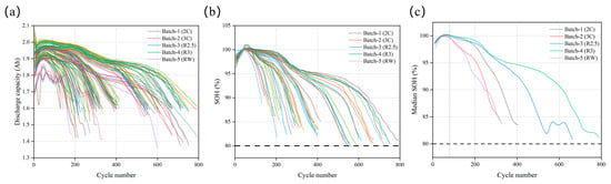
Figure 3 provides a descriptive visualization of the directly recorded discharge-capacity trajectories and the corresponding raw capacity-retention-based SOH characteristics of XJTU Batch-1 to Batch-5. These raw trajectories are used only to illustrate the observed degradation characteristics under different aging protocols, whereas the reconstructed SOH labels used for modeling are defined in Section 2.3 and summarized statistically in Table 2. The 80% SOH level is retained only as a visual reference and is not used for data filtering or model training.

Figure 3. Descriptive degradation characteristics of XJTU Batch-1 to Batch-5 based on the directly recorded cycle-level data: (a) discharge-capacity trajectories; (b) raw capacity-retention-based SOH trajectories; and (c) median raw SOH trends. Batch-1 and Batch-2 represent the 2C and 3C constant-current aging conditions, Batch-3 and Batch-4 represent the R2.5 and R3 dynamic aging conditions, and Batch-5 represents the RW random-walk condition. The dashed line denotes the 80% reference threshold.

3.3. Model Input Features

To improve the adaptability of the model to different aging conditions, this study does not rely on a single capacity indicator. Instead, cycle-level features are constructed from cycle state, capacity fading, energy variation, voltage response, local fluctuation, and degradation variation. The feature groups and their roles are summarized in Table 3.

Table 3. Model input feature groups and their roles.

Feature Group	Representative Variables	Use Scenario	Role
Cycle-position and condition-encoding features	cycle_index, batch_code, protocol_code	XJTU internal modeling	Describe cycle position and known aging-condition information
Capacity-related features	charge_capacity_Ah, charge_capacity_norm, and other non-target capacity descriptors	XJTU internal modeling	Provide non-target capacity-related degradation information
Energy-throughput features	charge_power_Wh, discharge_power_Wh, charge_power_norm, discharge_power_norm	XJTU internal modeling	Provide charge/discharge energy variation information
Voltage statistical features	charge_mean_voltage, discharge_mean_voltage, charge_median_voltage, discharge_median_voltage, charge_voltage_drop, discharge_voltage_drop, mean_voltage_gap	XJTU internal modeling; external validation feature alignment	Characterize voltage-response differences caused by aging and operating conditions
Local rolling-statistical features	charge_capacity_norm_roll5_mean, charge_capacity_norm_roll5_std, duration_s_roll5_mean, duration_s_roll5_std	XJTU internal modeling	Describe short-term fluctuation and local degradation state
First-order degradation-variation features	charge_capacity_norm_diff1, charge_power_norm_diff1, discharge_power_norm_diff1, charge_mean_voltage_diff1, discharge_mean_voltage_diff1, mean_voltage_gap_diff1	XJTU internal modeling	Represent degradation changes between adjacent cycles
Common feature subset for external validation	Cycle-related variables, voltage statistics, current/load statistics, temperature statistics, and time-related variables	XJTU–NASA external validation	Construct an aligned common feature space for cross-dataset validation

Note: cycle_norm, cycle_life_summary, battery identifiers, duplicate index fields, and target-defining capacity variables are excluded from model inputs to prevent future-information or identifier leakage.

Cycle-position and condition-encoding features used for modeling include cycle_index, batch_code, and protocol_code. The full-lifetime-normalized variable cycle_norm, the full-lifetime metadata field cycle_life_summary, and identifier-related metadata are explicitly excluded from model inputs to prevent future-information leakage and dependence on arbitrary cell identifiers.

Capacity-related information is used for target construction and degradation characterization. To avoid direct target leakage, the target-defining variables discharge_capacity_Ah and q0_discharge_capacity_Ah are explicitly excluded from model inputs. The retained non-target capacity descriptors are combined with energy, voltage, rolling-statistical, and first-order variation features to characterize battery degradation under different conditions.

Voltage statistical features characterize response differences caused by aging and operating conditions, while energy-throughput features describe changes in charge and discharge energy. Local rolling statistics and first-order degradation-variation features reflect short-term fluctuations and local degradation trends. The rolling-statistical features are calculated only from the current and previous cycles, without using future-cycle information.

For XJTU-to-NASA external validation, the recorded fields and test protocols of the two datasets are not fully consistent. Therefore, a common aligned feature space is constructed using cycle-related variables, voltage statistics, current/load statistics, temperature statistics, and time-related variables. Consequently, several XJTU-specific degradation features, including energy-throughput and several XJTU-specific rolling-statistical features, cannot be consistently retained. This loss of degradation-related information may contribute to the reduced cross-dataset transfer performance.

3.4. Data Distribution and Differences in External Validation Data

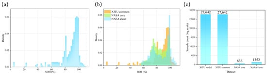
To clarify the distribution relationship between the training data and the external validation data, the SOH distribution, sample size, and representative degradation trajectories of the XJTU and NASA datasets are analyzed, as shown in Figure 4 and Figure 5. This section aims to describe the coverage of the training data and reveal the objective distribution differences in external validation, providing a basis for the subsequent cross-condition and cross-dataset analyses.

Figure 4. Descriptive SOH distribution and sample composition of the datasets based on the original cycle-level data: (a) raw SOH distribution of XJTU; (b) raw SOH distribution comparison among XJTU, NASA core, and NASA clean; (c) comparison of cycle sample numbers among different datasets.

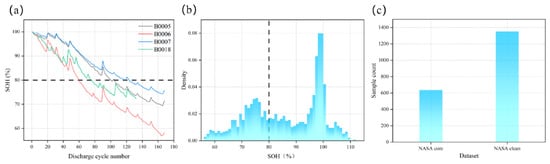
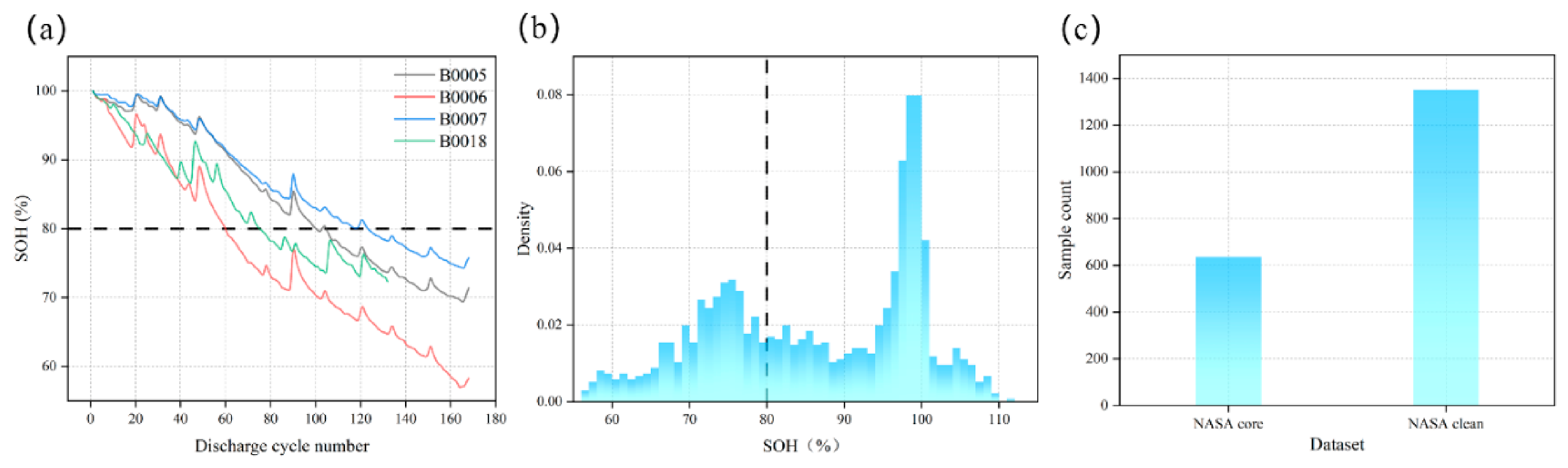
Figure 5. Characteristics of the NASA external validation data: (a) SOH degradation trajectories of representative cells in NASA core; (b) SOH distribution of NASA external validation samples; (c) comparison of cycle sample numbers between NASA core and NASA clean.

Figure 4 provides a descriptive comparison of the original cycle-level SOH distributions and sample composition across the XJTU and NASA datasets. The reconstructed XJTU SOH labels used for subsequent modeling are reported separately in Table 1. Despite differences in the detailed SOH distributions, XJTU and NASA retain a substantial overlapping health-state range, while NASA contains more low-SOH samples. Therefore, the external validation represents a cross-dataset transfer task rather than an in-distribution test.

Figure 4c shows the sample-size differences among the datasets. Both the XJTU modeling dataset and the XJTU common-feature dataset contain 27,642 cycle samples, while NASA core and NASA clean contain only 636 and 1352 cycle samples, respectively. This imbalance between the source training domain and the external test domain further increases the distribution-shift challenge. Thus, the NASA external validation results reflect not only model error, but also transfer stability under small-sample and out-of-distribution target domains.

Figure 5 further presents the degradation characteristics of the NASA external validation data. Figure 5a shows the SOH trajectories of four representative NASA core cells, namely B0005, B0006, B0007, and B0018. The cells differ in degradation rate, local fluctuation, and the cycle position at which they reach the 80% SOH reference threshold, indicating strong cell-to-cell variation within the NASA dataset. Compared with the XJTU data, the NASA cells show different cycle lengths, degradation slopes, and local fluctuation patterns, reflecting differences caused by test platforms and experimental protocols.

Figure 5b shows the SOH distribution of the NASA external validation samples. Overall, the NASA samples are mainly concentrated in the middle-to-high SOH range, while also covering some degraded samples below 80% SOH. This enables evaluation of external applicability across different health stages. Figure 5c compares the sample sizes of NASA core and NASA clean. NASA clean contains more samples and is used as an extended external validation set with a larger scale and more complex distribution. NASA core is smaller but contains four commonly used benchmark cells, making it suitable for core comparative analysis. Overall, XJTU and NASA differ in sample size, SOH distribution, and degradation trajectory. Therefore, NASA external validation is used as a supplementary test of cross-dataset generalization and model limitations, rather than being treated as equivalent to XJTU internal cross-condition testing.

3.5. Experimental Splits

To evaluate SOH estimation under different generalization scenarios, three experimental tasks are designed: cell-wise internal validation, condition-wise cross-condition validation, and NASA external validation. The detailed splits are listed in Table 4. Cell-wise validation evaluates generalization to unseen cells, condition-wise validation evaluates adaptability to an unseen aging condition, and NASA external validation examines cross-dataset transfer performance.

Table 4. Experimental splits and evaluation settings.

Evaluation Setting	Training Set	Test Set	Training Samples/Cells	Test Samples/Cells
Cell-wise internal validation	XJTU modeling dataset	XJTU modeling dataset	21,052/42	6590/13
Condition-wise validation	XJTU Batch-1 to Batch-5	XJTU Batch-6	19,238/47	8404/8
NASA core external validation	XJTU common-feature dataset	NASA core dataset	27,642/55	636/4
NASA clean external validation	XJTU common-feature dataset	NASA clean dataset	27,642/55	1352/17

Cell-wise internal validation is conducted within the XJTU modeling dataset. The data are divided by cell ID, with 42 cells and 21,052 cycle samples for training and 13 cells and 6590 cycle samples for testing. Cycle samples from the same cell do not appear in both training and test sets, avoiding cell-level information leakage. Since the training and test sets are from the same dataset and have relatively similar condition distributions, this split mainly reflects cell-level generalization under near-domain conditions.

Condition-wise validation uses XJTU Batch-1 to Batch-5 as the training set, including 47 cells and 19,238 cycle samples, and uses Batch-6 as the test set, including 8 cells and 8404 cycle samples. Batch-6 corresponds to the Sim_satellite condition and differs from the other batches in cycle span and degradation characteristics. This split is therefore used to test cross-condition generalization from constant-current, dynamic, and random-walk aging conditions to simulated satellite operation. The subsequent model comparison, branch contribution analysis, and ablation study mainly focus on this setting.

For NASA external validation, models are trained on the XJTU common-feature dataset and tested on NASA core and NASA clean, respectively. NASA core contains 4 cells and 636 cycle samples for core external validation, while NASA clean contains 17 cells and 1352 cycle samples for extended external validation. Since XJTU and NASA differ in cell type, test protocol, recorded fields, and SOH distribution, only the aligned XJTU–NASA common feature space is used. This validation mainly analyzes model transferability and limitations under out-of-distribution data.

All experiments use MAE, RMSE, MAPE, and R² as evaluation metrics, with RMSE as the primary comparison metric. To prevent data leakage, all data-dependent preprocessing parameters, including missing-value imputation and standardization where required, are determined only from the corresponding training set and then applied unchanged to the test or external validation set. The test and external validation sets are not used for model training, standardization-parameter calculation, or hyperparameter selection.

4. Results and Analysis

4.1. SOH Estimation Results Under XJTU Cross-Condition Validation

To evaluate SOH estimation performance under an unseen aging condition, condition-wise validation is conducted on the XJTU dataset. Batches 1 to 5 are used as the training set, while Batch-6 under the Sim_satellite condition is used as the test set. Compared with the cell-wise split, this setting involves different aging protocols between training and testing, and therefore better reflects the model’s extrapolation ability under unseen conditions.

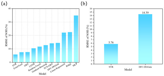
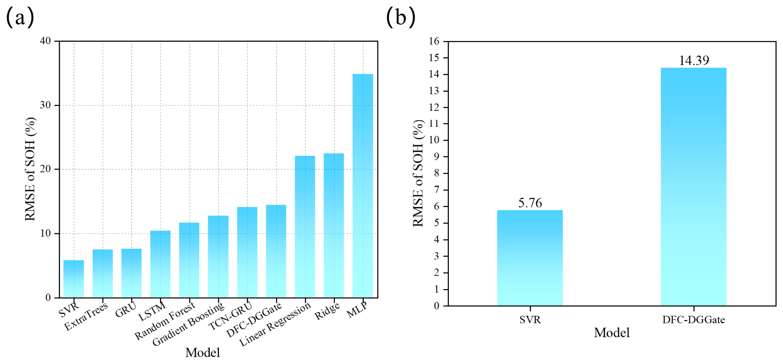
Figure 6 and Table 5 compare the performance of different models under the condition-wise split. SVR achieves the lowest RMSE of 5.7623%, followed by ExtraTrees (7.4705%) and GRU (7.5523%). DFC-DGGate obtains an RMSE of 14.3895%, outperforming Linear Regression, Ridge, and MLP, but not the strongest nonlinear and sequence baselines. These results indicate that the current fixed condition-level routing strategy remains sensitive to the substantial Sim_satellite distribution shift.

Figure 6. Performance comparison of different SOH estimation models under the XJTU cross-condition split: (a) RMSE comparison of different models under the condition-wise split; (b) RMSE comparison between the best baseline model and DFC-DGGate.

Table 5. Performance comparison of different SOH estimation models under the XJTU cross-condition split.

Rank	Model	Model Type	RMSE (%)
1	SVR	Kernel-based method	5.7623
2	ExtraTrees	Tree-based model	7.4705
3	GRU	Deep learning model	7.5523
4	LSTM	Deep learning model	10.3742
5	Random Forest	Tree-based model	11.5995
6	Gradient Boosting	Tree-based model	12.7097
7	TCN-GRU	Deep learning model	14.0515
8	DFC-DGGate	Proposed method	14.3895
9	Linear Regression	Linear model	22.0147
10	Ridge	Linear model	22.3915
11	MLP	Deep learning model	34.8384

As discussed in Section 3.2, Batch-6 differs substantially from the training batches in operating protocol, cycle span, and SOH distribution. The revised comparison shows that nonlinear models generalize more effectively than the global linear models in this setting: Ridge and Linear Regression yield RMSE values above 22%, whereas SVR, ExtraTrees, and GRU show substantially lower errors. This indicates that the Sim_satellite shift cannot be adequately represented by a simple global linear degradation relationship and also reveals the limitation of using fixed routing coefficients under a strong unseen-condition shift.

Overall, the condition-wise results show that DFC-DGGate provides an interpretable multi-branch estimate under an unseen aging condition but does not outperform the strongest nonlinear baselines under the substantial Sim_satellite shift. The following sections further examine the branch contributions and the limitations of the current gating strategy.

4.2. Branch Contribution Analysis

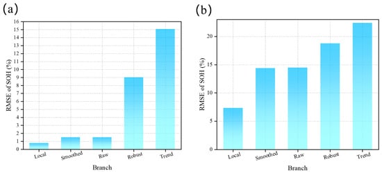
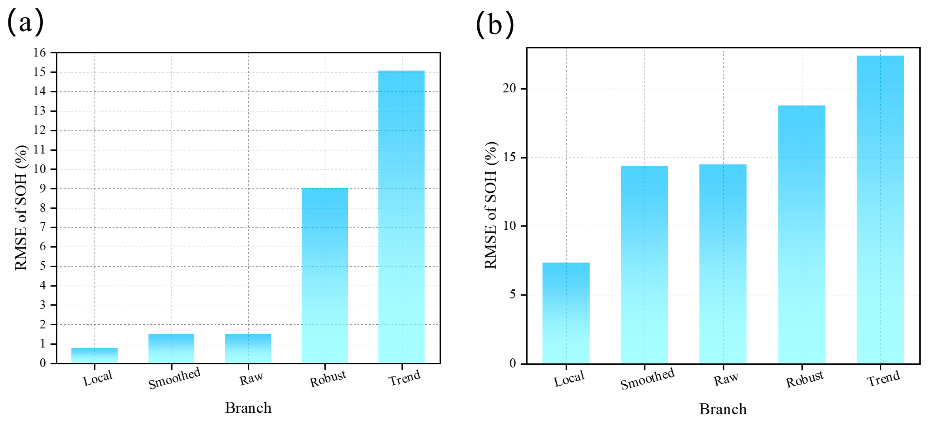
To analyze the effects of different branches and gated outputs in DFC-DGGate, the RMSE values of Local ET, Robust Huber, Trend Ridge, Raw gate, and Smoothed gate are compared under both cell-wise and condition-wise splits. The results are shown in Figure 7 and Table 6. Raw gate denotes the gated fusion output without smoothing, while Smoothed gate denotes the final output after the smoothing module.

Figure 7. SOH estimation performance comparison of different DFC-DGGate branches: (a) RMSE comparison under the cell-wise split; (b) RMSE comparison under the condition-wise split.

Table 6. Performance comparison of different DFC-DGGate branches.

Split	Branch	RMSE (%)
Cell-wise	Local ET	0.7701
Cell-wise	Smoothed gate	1.4841
Cell-wise	Raw gate	1.4990
Cell-wise	Robust Huber	9.0184
Cell-wise	Trend Ridge	15.0834
Condition-wise	Local ET	7.3129
Condition-wise	Smoothed gate	14.3895
Condition-wise	Raw gate	14.4771
Condition-wise	Robust Huber	18.7470
Condition-wise	Trend Ridge	22.3915

Under the cell-wise split, Local ET achieves the lowest branch-level RMSE of 0.7701%. Raw gate and Smoothed gate obtain RMSE values of 1.4990% and 1.4841%, respectively, while Robust Huber and Trend Ridge yield substantially larger RMSE values of 9.0184% and 15.0834%. These results indicate that local nonlinear mapping dominates under near-domain unseen-cell testing, while smoothing produces only a small change in the gated output.

Under the condition-wise split, Local ET achieves the lowest branch-level RMSE of 7.3129%, whereas Robust Huber and Trend Ridge yield RMSE values of 18.7470% and 22.3915%, respectively. Raw gate obtains an RMSE of 14.4771%, and smoothing slightly reduces it to 14.3895%. The LOCO-calibrated unseen routing assigns equal weight to Local ET and Trend Ridge and zero weight to Robust Huber, indicating that the relative usefulness of the branches changes substantially under the Sim_satellite condition.

These results show that Local ET remains the strongest individual branch in both validation settings. The condition-aware gate performs better than simple equal weighting but does not surpass Local ET under the strong Sim_satellite shift. In particular, the training-domain LOCO calibration retains a substantial Trend Ridge contribution that is not optimal for Batch-6, revealing an important limitation of the current fixed routing strategy.

4.3. Ablation Study

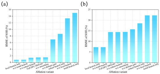
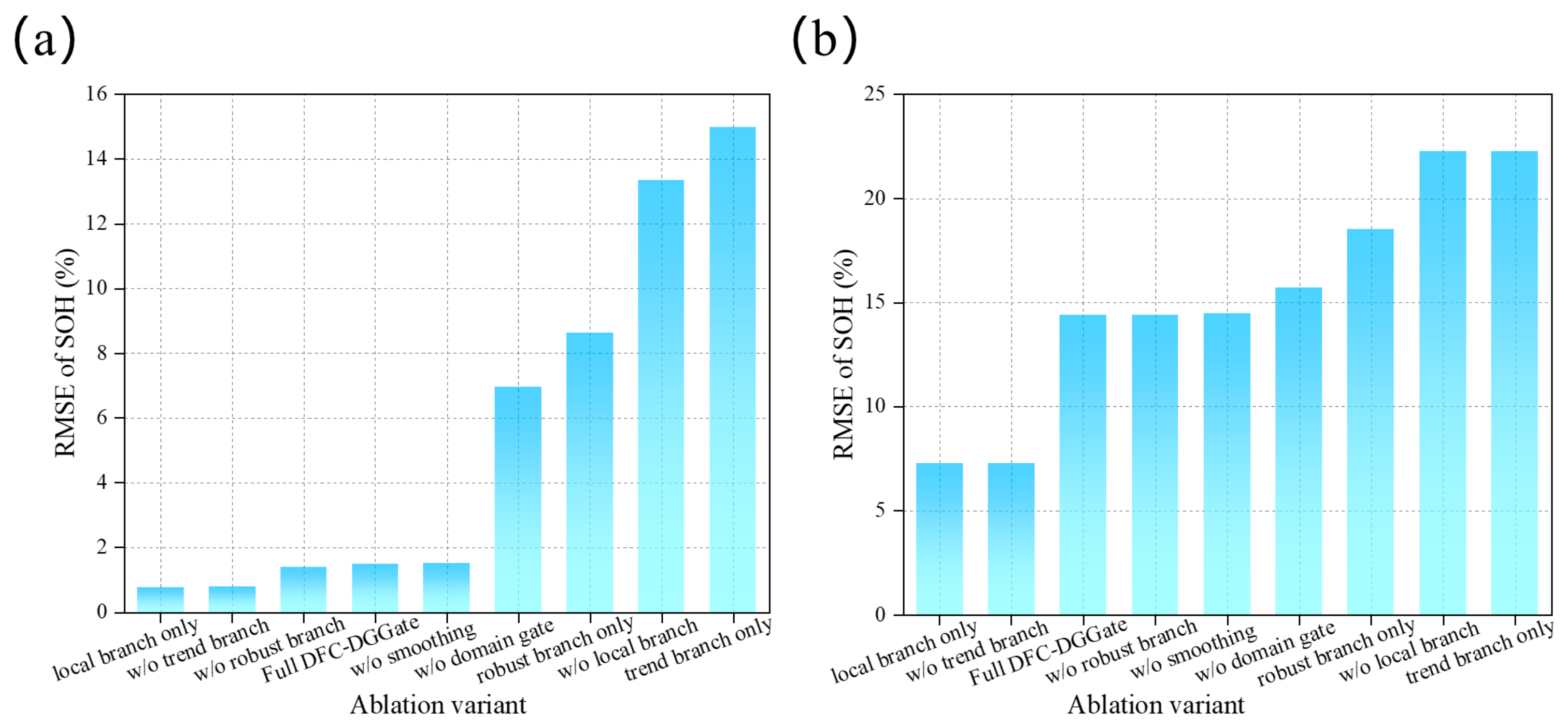
To further verify the contribution of each component in DFC-DGGate to SOH estimation performance, ablation experiments are conducted under both cell-wise and condition-wise splits. Different from the branch contribution analysis in Section 4.2, this section focuses on the performance changes after removing the smoothing module, the domain-difference gate, or one estimation branch from the full model. All ablation variants use the same data splits as the full model. RMSE is used as the primary metric, while MAE and R² are additionally reported in Table 7 to provide complementary evaluation of the ablation results. The results are shown in Figure 8 and Table 7.

Table 7. Ablation results of DFC-DGGate.

Split	Ablation Variant	MAE (%)	RMSE (%)	R2
Cell-wise	local branch only	0.3501	0.7711	0.9840
Cell-wise	w/o trend branch	0.3370	0.7852	0.9835
Cell-wise	w/o robust branch	0.5841	1.3976	0.9476
Cell-wise	Full DFC-DGGate	0.6101	1.4841	0.9409
Cell-wise	w/o smoothing	0.6110	1.4990	0.9397
Cell-wise	w/o domain gate	2.4100	6.9500	−0.2964
Cell-wise	robust branch only	2.6575	8.6320	−0.9998
Cell-wise	w/o local branch	4.6040	13.3475	−3.7815
Cell-wise	trend branch only	5.1401	14.9938	−5.0337
Condition-wise	local branch only	6.0203	7.2685	−1.5965
Condition-wise	w/o trend branch	6.0203	7.2685	−1.5965
Condition-wise	Full DFC-DGGate	11.3729	14.3895	−9.1765
Condition-wise	w/o robust branch	11.3729	14.3895	−9.1765
Condition-wise	w/o smoothing	11.3784	14.4771	−9.3007
Condition-wise	w/o domain gate	12.2699	15.7140	−11.1360
Condition-wise	robust branch only	14.1446	18.5163	−15.8505
Condition-wise	w/o local branch	16.9579	22.2428	−23.3154
Condition-wise	trend branch only	16.9579	22.2428	−23.3154

Figure 8. Ablation results of DFC-DGGate: (a) RMSE comparison of different ablation variants under the cell-wise split; (b) RMSE comparison of different ablation variants under the condition-wise split.

Under the cell-wise split, the full DFC-DGGate achieves an RMSE of 1.4841%. The local-branch-only and w/o-trend variants achieve RMSE values of 0.7711% and 0.7852%, respectively. Removing the Domain gate substantially increases the RMSE to 6.9500%, whereas removing the Local branch increases it to 13.3475%. These results indicate that Local ET is the dominant branch under near-domain testing, while condition-aware routing is substantially more effective than simple equal weighting.

Under the condition-wise split, the full DFC-DGGate achieves an RMSE of 14.3895%. The local-branch-only variant achieves the lowest RMSE of 7.2685%, while removing the Domain gate increases the RMSE to 15.7140%. Because the LOCO-calibrated unseen-condition routing assigns zero weight to Robust Huber, removing the Robust branch does not change the full-model prediction, and removing the Trend branch becomes equivalent to the local-only variant. These results confirm that condition-aware routing improves upon equal weighting but also show that the current fixed unseen-condition weights do not fully adapt to the strong Sim_satellite shift.

A sensitivity analysis of α was also conducted. For α = 0.85, 0.90, 0.92, 0.94, 0.95, and 0.98, the condition-wise RMSE values are 14.3201%, 14.3691%, 14.3895%, 14.4105%, 14.4212%, and 14.4543%, respectively. The relatively small variation across this range indicates that the model is not highly sensitive to α. Therefore, α = 0.92 is retained as a conservative light-smoothing setting rather than as a finely tuned optimum.

Overall, the ablation results show that the contribution of each component depends strongly on the domain shift. Local ET provides the dominant predictive information, while the Domain gate improves substantially upon simple equal weighting. However, the fixed LOCO-calibrated routing does not consistently outperform the strongest individual branch. These results motivate more continuous and data-driven estimation of branch reliability in future work.

4.4. Cross-Dataset Validation on NASA Data

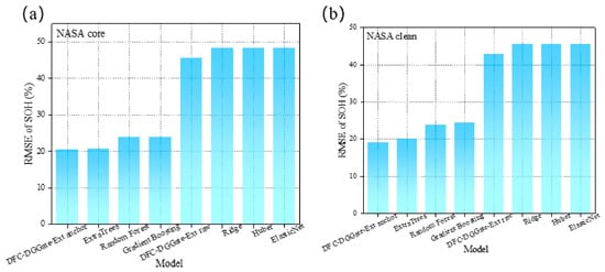
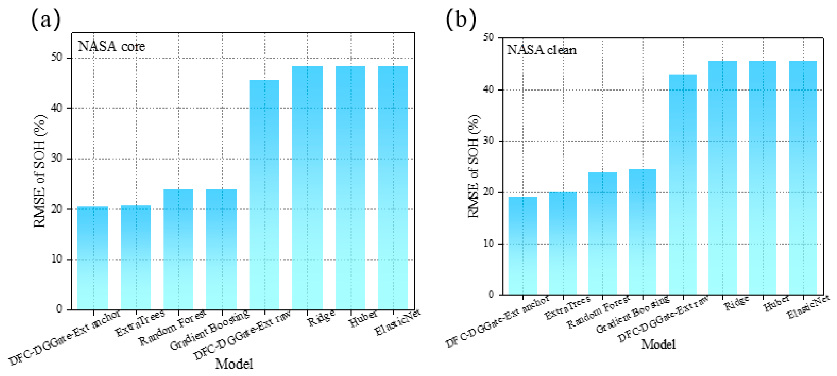
In this study, cross-condition generalization refers to transfer across different aging conditions within the XJTU dataset, whereas cross-dataset generalization refers to transfer from XJTU to the independently sourced NASA dataset. To evaluate the applicability of the models under cross-dataset conditions, the XJTU common-feature dataset is used as the training set, while NASA core and NASA clean are used as external test sets. Since XJTU and NASA differ in cell type, test protocol, recorded variables, and SOH distribution, this experiment mainly examines model transferability and limitations under out-of-distribution data. The results are shown in Figure 9 and Table 8.

Figure 9. SOH estimation performance comparison in XJTU-to-NASA external validation: (a) RMSE comparison on the NASA core dataset; (b) RMSE comparison on the NASA clean dataset.

Table 8. XJTU-to-NASA external validation results.

External Validation Dataset	Model	Model Type	RMSE (%)
NASA core	DFC-DGGate-Ext anchor	Gated extension model	20.45
NASA core	ExtraTrees	Tree-based model	20.80
NASA core	Random Forest	Tree-based model	23.89
NASA core	Gradient Boosting	Tree-based model	23.90
NASA core	DFC-DGGate-Ext raw	Gated extension model	45.53
NASA core	Ridge	Linear model	48.40
NASA core	Huber	Linear model	48.40
NASA core	ElasticNet	Linear model	48.40
NASA clean	DFC-DGGate-Ext anchor	Gated extension model	19.10
NASA clean	ExtraTrees	Tree-based model	20.08
NASA clean	Random Forest	Tree-based model	23.89
NASA clean	Gradient Boosting	Tree-based model	24.57
NASA clean	DFC-DGGate-Ext raw	Gated extension model	42.77
NASA clean	Huber	Linear model	45.53
NASA clean	Ridge	Linear model	45.55
NASA clean	ElasticNet	Linear model	45.55

On NASA core, DFC-DGGate-Ext anchor achieves the lowest RMSE of 20.45%, followed closely by ExtraTrees at 20.80%, while Random Forest and Gradient Boosting obtain 23.89% and 23.90%, respectively. The raw external extension yields a much larger RMSE of 45.53%. On NASA clean, DFC-DGGate-Ext anchor again achieves the lowest RMSE of 19.10%, followed by ExtraTrees at 20.08%, while Random Forest and Gradient Boosting obtain 23.89% and 24.57%, respectively. The raw external result has an RMSE of 42.77%. These results show that the initial-window anchor correction substantially reduces cross-dataset offset; however, the large raw-transfer errors also indicate that the external improvement relies strongly on this calibration and should not be interpreted as complete domain invariance.

These results confirm that cross-condition and cross-dataset generalization are not equivalent. The strong performance of ExtraTrees indicates that flexible nonlinear partitioning remains effective in the reduced common feature space. The anchor-corrected external extension slightly improves upon ExtraTrees on both NASA subsets, but its much weaker raw-transfer performance shows that substantial cross-dataset offset remains. Therefore, cross-condition and cross-dataset generalization should still be treated as distinct problems.

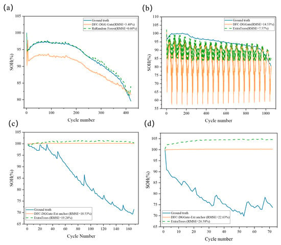
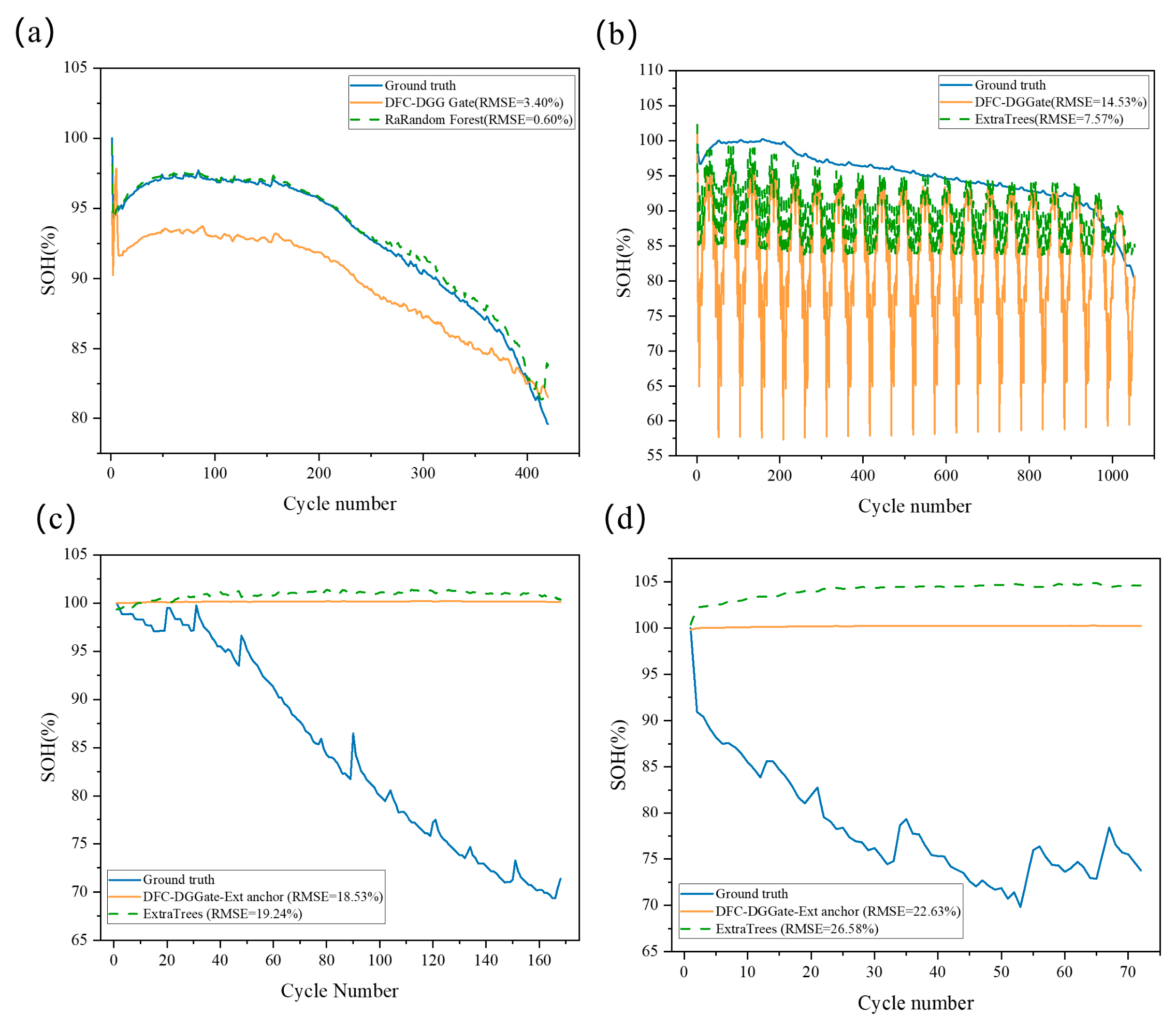
Figure 10 provides representative trajectory-level comparisons between the ground-truth SOH and model predictions under all four validation settings. The cell-wise results show that both DFC-DGGate and the benchmark closely follow the overall degradation trajectory. Under the more challenging condition-wise and NASA external settings, larger prediction deviations are observed, indicating that increasing condition and dataset shifts substantially affect trajectory-level generalization. These results complement the scalar error metrics and provide a more transparent assessment of both prediction capability and remaining transfer limitations.

Figure 10. Representative ground-truth and predicted SOH trajectories under the four validation settings: (a) cell-wise internal validation; (b) condition-wise cross-condition validation; (c) NASA core external validation; and (d) NASA clean external validation. The proposed method is compared with a representative strong benchmark under each setting.

5. Discussion

The results show that no single model dominates across all validation settings. Under the XJTU condition-wise split, SVR achieves the lowest RMSE of 5.7623%, whereas DFC-DGGate obtains 14.3895%. Local ET also outperforms the full gated model, indicating that the reliability of different branches changes considerably under the Sim_satellite shift. Therefore, combining complementary branches alone is insufficient when fixed routing coefficients cannot accurately reflect the target-domain branch reliability.

The branch and ablation results further clarify this limitation. The Domain gate substantially improves upon simple equal weighting, but the LOCO-calibrated unseen-condition vector assigns equal contributions to Local ET and Trend Ridge while suppressing Robust Huber. This routing is effective on average across the training-domain LOCO folds but remains suboptimal for Batch-6, where Local ET alone performs considerably better. Future gating strategies should therefore characterize domain discrepancy and branch reliability more continuously rather than relying only on a binary seen/unseen condition indicator.

Recent studies have addressed battery-health generalization and robust prediction from different perspectives. Chen et al. [20] investigated transfer learning under domain shift, while Dou et al. [21] and Zhu et al. [22] explored latent-space consistency and domain-adaptive learning for cross-domain battery health estimation. Zeng et al. [23] and Lin et al. [24] further investigated ensemble and physics-informed learning under varying operating conditions. Jiang et al. [18,19] developed flexible parallel neural-network architectures for early battery-lifespan and RUL prediction with limited observations, highlighting the value of adaptive multi-branch structures. In contrast, DFC-DGGate uses a lightweight staged fusion of nonlinear, robust, and trend branches with explicit condition-level routing. The present results show improved performance over simple equal weighting and transparent branch contributions, but also reveal that fixed routing remains insufficient under the severe Sim_satellite shift. Because these studies differ in prediction targets, datasets, and validation protocols, direct numerical comparison is not appropriate.

The NASA external validation reveals a different behavior. After feature alignment, the raw external extension shows large prediction offsets, whereas the initial-window anchor correction reduces RMSE to 20.45% on NASA core and 19.10% on NASA clean, slightly outperforming ExtraTrees on both subsets. This result demonstrates the practical value of limited target-domain initialization, but also shows that the improvement is primarily associated with offset correction rather than complete cross-dataset invariance. Differences in feature availability, cell chemistry/design, cycling protocols, aging mechanisms, and SOH distributions therefore remain important sources of transfer difficulty.

This study still has several limitations. First, the XJTU internal model uses 35 input features, whereas XJTU-to-NASA external validation uses 51 aligned features. The two feature spaces are not strictly nested because the external feature space is reconstructed from variables jointly available in XJTU and NASA, and some XJTU-specific features cannot be directly transferred. Second, the current task is mainly positioned as cycle-level SOH estimation under capacity-available conditions. The model performance after removing direct capacity-related features should be further examined. Third, explicit domain adaptation or few-shot target-domain calibration has not yet been incorporated. Future work will focus on chemistry- and protocol-aware domain descriptors, degradation features that can be consistently measured across datasets, and explicit domain-adaptation or limited target-domain calibration strategies. Multi-source battery datasets covering different chemistries and aging mechanisms will also be incorporated to improve cross-dataset generalization.

6. Conclusions

This study addresses the limited generalization of SOH estimation models under unseen aging conditions and proposes DFC-DGGate, a degradation-feature-constrained domain-difference gated method for lithium-ion power batteries. The method uses cycle-level degradation features as inputs and constructs three branches, namely Local ET, Trend Ridge, and Robust Huber, to characterize local nonlinear relationships, global degradation trends, and robustness against abnormal fluctuations. A domain-difference gate and a smoothing module are then used for condition-aware fusion and temporal stabilization of the branch outputs.

Experiments on the XJTU dataset show that DFC-DGGate provides an interpretable multi-branch framework for SOH estimation under changing aging conditions, but its performance remains sensitive to severe unseen-condition shifts. Under the Sim_satellite condition, the full gated model does not outperform SVR, ExtraTrees, or the Local ET branch, revealing an important applicability boundary of the current fixed routing strategy.

The branch and ablation analyses show that Local ET provides the strongest individual-branch performance, while condition-aware routing substantially improves upon simple equal weighting. However, the LOCO-calibrated fixed weights do not consistently match the branch reliability of a strongly shifted target condition. Future improvements should therefore focus on continuous domain-discrepancy assessment and data-driven branch-reliability estimation.

The NASA external validation further shows that limited target-domain initialization can substantially reduce cross-dataset offset. The anchor-corrected external extension achieves slightly lower RMSE than ExtraTrees on both NASA subsets, whereas the raw transfer remains considerably less accurate. From an engineering perspective, DFC-DGGate provides an interpretable framework for combining complementary SOH estimators, but further domain-aware calibration, multi-source validation, and onboard implementation are required before practical deployment in vehicle battery management systems.

References

- Sui, X.; He, S.; Vilsen, S.B.; Meng, J.; Teodorescu, R.; Stroe, D.-I. A review of non-probabilistic machine learning-based state of health estimation techniques for Lithium-ion battery. Appl. Energy 2021, 300, 117346. [Google Scholar] [CrossRef] [Scilit]
- Vennam, G.; Sahoo, A.; Ahmed, S. A survey on lithium-ion battery internal and external degradation modeling and state of health estimation. J. Energy Storage 2022, 52, 104720. [Google Scholar] [CrossRef] [Scilit]
- Luo, K.; Chen, X.; Zheng, H.; Shi, Z. A review of deep learning approach to predicting the state of health and state of charge of lithium-ion batteries. J. Energy Chem. 2022, 74, 159–173. [Google Scholar] [CrossRef] [Scilit]
- Li, P.; Zhang, Z.; Grosu, R.; Deng, Z.; Hou, J.; Rong, Y.; Wu, R. An end-to-end neural network framework for state-of-health estimation and remaining useful life prediction of electric vehicle lithium batteries. Renew. Sustain. Energy Rev. 2022, 156, 111843. [Google Scholar] [CrossRef] [Scilit]
- Tian, J.; Xiong, R.; Shen, W.; Lu, J.; Sun, F. Flexible battery state of health and state of charge estimation using partial charging data and deep learning. Energy Storage Mater. 2022, 51, 372–381. [Google Scholar] [CrossRef] [Scilit]
- Hong, J.; Wang, Z.; Chen, W.; Wang, L.; Lin, P.; Qu, C. Online accurate state of health estimation for battery systems on real-world electric vehicles with variable driving conditions considered. J. Clean. Prod. 2021, 294, 125814. [Google Scholar] [CrossRef] [Scilit]
- Chen, Z.; Zhao, H.; Zhang, Y.; Shen, S.; Shen, J.; Liu, Y. State of health estimation for lithium-ion batteries based on temperature prediction and gated recurrent unit neural network. J. Power Sources 2022, 521, 230892. [Google Scholar] [CrossRef] [Scilit]
- Ma, Y.; Shan, C.; Gao, J.; Chen, H. A novel method for state of health estimation of lithium-ion batteries based on improved LSTM and health indicators extraction. Energy 2022, 251, 123973. [Google Scholar] [CrossRef] [Scilit]
- Bockrath, S.; Lorentz, V.; Pruckner, M. State of health estimation of lithium-ion batteries with a temporal convolutional neural network using partial load profiles. Appl. Energy 2023, 329, 120307. [Google Scholar] [CrossRef] [Scilit]
- Gu, X.; See, K.; Li, P.; Shan, K.; Wang, Y.; Zhao, L.; Lim, K.C.; Zhang, N. A novel state-of-health estimation for the lithium-ion battery using a convolutional neural network and transformer model. Energy 2023, 262, 125501. [Google Scholar] [CrossRef] [Scilit]
- Zhang, Z.; Min, H.; Guo, H.; Yu, Y.; Sun, W.; Jiang, J.; Zhao, H. State of health estimation method for lithium-ion batteries using incremental capacity and long short-term memory network. J. Energy Storage 2023, 64, 107063. [Google Scholar] [CrossRef] [Scilit]
- Gismero, A.; Nørregaard, K.; Johnsen, B.; Stenhøj, L.; Stroe, D.-I.; Schaltz, E. Electric vehicle battery state of health estimation using Incremental Capacity Analysis. J. Energy Storage 2023, 64, 107110. [Google Scholar] [CrossRef] [Scilit]
- Feng, X.; Zhang, Y.; Xiong, R.; Wang, C. Comprehensive performance comparison among different types of features in data-driven battery state of health estimation. Appl. Energy 2024, 369, 123555. [Google Scholar] [CrossRef] [Scilit]
- Wang, T.; Ma, Z.; Zou, S.; Chen, Z.; Wang, P. Lithium-ion battery state-of-health estimation: A self-supervised framework incorporating weak labels. Appl. Energy 2024, 355, 122332. [Google Scholar] [CrossRef] [Scilit]
- Wang, F.; Zhai, Z.; Zhao, Z.; Di, Y.; Chen, X. Physics-informed neural network for lithium-ion battery degradation stable modeling and prognosis. Nat. Commun. 2024, 15, 4332. [Google Scholar] [CrossRef] [Scilit] [PubMed]
- Yu, Q.; Nie, Y.; Liu, S.; Li, J.; Tang, A. State of health estimation method for lithium-ion batteries based on multiple dynamic operating conditions. J. Power Sources 2023, 582, 233541. [Google Scholar] [CrossRef] [Scilit]
- Chen, X.; Qin, Y.; Zhao, W.; Yang, Q.; Cai, N.; Wu, K. A self-attention knowledge domain adaptation network for commercial lithium-ion batteries state-of-health estimation under shallow cycles. J. Energy Storage 2024, 86, 111197. [Google Scholar] [CrossRef] [Scilit]
- Jiang, L.; Li, Z.; Hu, C.; Chen, J.; Huang, Q.; He, G. A robust adapted flexible parallel neural network architecture for early prediction of lithium battery lifespan. Energy 2024, 308, 132840. [Google Scholar] [CrossRef] [Scilit]
- Jiang, L.; Huang, Q.; He, G. Predicting the remaining useful life of lithium-ion batteries using 10 random data points and a flexible parallel neural network. Energies 2024, 17, 1695. [Google Scholar] [CrossRef] [Scilit]
- Chen, X.; Sun, T.; Lai, X.; Zheng, Y.; Han, X. Transfer learning strategies for lithium-ion battery capacity estimation under domain shift differences. J. Energy Storage 2024, 90, 111860. [Google Scholar] [CrossRef] [Scilit]
- Dou, B.; Hou, S.; Li, H.; Zhao, Y.; Fan, Y.; Sun, L.; Chen, H.-S. Cross-domain state of health estimation for lithium-ion battery based on latent space consistency using few-unlabeled data. Energy 2025, 320, 135257. [Google Scholar] [CrossRef] [Scilit]
- Zhu, B.; Jia, L.; Pan, Q.; Zhang, H. Cross-domain battery SOH and RUL estimation via Domain-Adaptive Transformer. Energy 2025, 341, 139288. [Google Scholar] [CrossRef] [Scilit]
- Zeng, C.; Xu, C.; Li, H.; Wang, K. A novel ensemble learning model for state of health estimation of lithium-ion batteries. J. Power Sources 2025, 638, 236608. [Google Scholar] [CrossRef] [Scilit]
- Lin, C.; Tuo, X.; Wu, L.; Zhang, G.; Lyu, Z.; Zeng, X. Physics-informed machine learning for accurate SOH estimation of lithium-ion batteries considering various temperatures and operating conditions. Energy 2025, 318, 134937. [Google Scholar] [CrossRef] [Scilit]
- Wang, F.; Zhai, Z.; Liu, B.; Zheng, S.; Zhao, Z.; Chen, X. Open access dataset, code library and benchmarking deep learning approaches for state-of-health estimation of lithium-ion batteries. J. Energy Storage 2024, 77, 109884. [Google Scholar] [CrossRef] [Scilit]
- Saha, B.; Goebel, K. Battery Data Set; NASA Prognostics Data Repository, NASA Ames Research Center: Moffett Field, CA, USA, 2007. Available online: https://www.nasa.gov/intelligent-systems-division/discovery-and-systems-health/pcoe/pcoe-data-set-repository/ (accessed on 1 August 2026).
- Hoerl, A.E.; Kennard, R.W. Ridge regression: Biased estimation for nonorthogonal problems. Technometrics 1970, 12, 55–67. [Google Scholar] [CrossRef]
- Huber, P.J. Robust estimation of a location parameter. Ann. Math. Stat. 1964, 35, 73–101. [Google Scholar] [CrossRef] [Scilit]
- Geurts, P.; Ernst, D.; Wehenkel, L. Extremely randomized trees. Mach. Learn. 2006, 63, 3–42. [Google Scholar] [CrossRef] [Scilit]
- Breiman, L. Random forests. Mach. Learn. 2001, 45, 5–32. [Google Scholar] [CrossRef] [Scilit]
- Friedman, J.H. Greedy function approximation: A gradient boosting machine. Ann. Stat. 2001, 29, 1189–1232. [Google Scholar] [CrossRef] [Scilit]
- Drucker, H.; Burges, C.J.C.; Kaufman, L.; Smol, A.; Vapoik, V. Support vector regression machines. Adv. Neural Inform. Process. Syst. 1997, 9, 155–161. [Google Scholar]
- Hochreiter, S.; Schmidhuber, J. Long short-term memory. Neural Comput. 1997, 9, 1735–1780. [Google Scholar] [CrossRef] [Scilit] [PubMed]
- Cho, K.; van Merriënboer, B.; Gulcehre, C.; Bahdanau, D.; Bougares, F.; Schwenk, H.; Bengio, Y. Learning phrase representations using RNN encoder–decoder for statistical machine translation. In Proceedings of the 2014 Conference on Empirical Methods in Natural Language Processing, Doha, Qatar, 25–29 October 2014; pp. 1724–1734. [Google Scholar]
- Bai, S.; Kolter, J.Z.; Koltun, V. An empirical evaluation of generic convolutional and recurrent networks for sequence modeling. arXiv 2018, arXiv:1803.01271. [Google Scholar]
- Pedregosa, F.; Varoquaux, G.; Gramfort, A.; Michel, V.; Thirion, B.; Grisel, O.; Blondel, M.; Prettenhofer, P.; Weiss, R.; Dubourg, V.; et al. Scikit-learn: Machine learning in Python. J. Mach. Learn. Res. 2011, 12, 2825–2830. [Google Scholar]
Disclaimer/Publisher’s Note: The statements, opinions and data contained in all publications are solely those of the individual author(s) and contributor(s) and not of MDPI and/or the editor(s). MDPI and/or the editor(s) disclaim responsibility for any injury to people or property resulting from any ideas, methods, instructions or products referred to in the content. |
© 2026 by the authors. Licensee MDPI, Basel, Switzerland. This article is an open access article distributed under the terms and conditions of the Creative Commons Attribution (CC BY) license.