Mission-Phase Feature Learning for eVTOL Li-Ion Battery Prognostics: A Leakage-Safe Cell-Held-Out Benchmark for SOC, SOH, and RUL

Abstract

Reliable battery prognostics for electric vertical take-off and landing (eVTOL) aircraft require models that preserve phase-dependent electrothermal information while generalizing to cells absent from training. This study reconstructs the public CMU eVTOL battery dataset and establishes a leakage-safe benchmark for state of charge (SOC), five-mission-ahead state of health (SOH), and threshold-based remaining useful life (RUL). A protocol-based screen identified 441 valid C/5 reference-performance-test anchors across 22 cells; three cells with non-monotone diagnostic-capacity trajectories were excluded from the primary health benchmark, leaving 19 cells. Predictors were restricted to telemetry-derived phase and mission features, with cell identity and target- or future-derived quantities excluded. All health models were evaluated using outer leave-one-cell-out validation with matched 20-mission histories. Random Forest achieved the lowest SOH MAE of 0.620 percentage points, compared with 1.252 for the mission-phase Transformer and 1.471 for Attention-LSTM-MoE. The best RUL MAEs were 24.067, 46.527, and 122.198 missions at the 90%, 85%, and 80% SOH thresholds. Cell-bootstrap uncertainty showed that model differences were threshold-dependent. Row-random splitting produced substantially more optimistic errors than cell-held-out evaluation. These results show that rigorous target construction and leakage-safe validation are critical and that increased sequence-model complexity does not guarantee superior unseen-cell generalization.

1. Introduction

Electric vertical take-off and landing (eVTOL) aircraft expose lithium-ion batteries to highly structured and rapidly changing duty cycles. Take-off and landing impose short, high-power demands, cruise produces a lower but sustained discharge load, and rapid turnaround may couple repeated flight missions with high-rate charging and an elevated state of charge. Consequently, current, voltage, temperature, and energy trajectories depend strongly on mission phase. Prognostic features that preserve phase identity can therefore represent local voltage sag, thermal response, charge acceptance, power demand, and cumulative energy exposure more explicitly than whole-mission aggregation alone. The publicly available CMU eVTOL battery dataset provides cell-level telemetry under representative flight-like and charging conditions and offers a suitable basis for evaluating such phase-aware prognostic approaches [1].

Existing eVTOL battery studies have demonstrated that engineered charging, discharging, temperature, and mission-profile descriptors can support SOH and RUL prediction [2,3]. Recent battery-prognostics research has additionally explored transfer learning, attention mechanisms, Transformer-based estimation, and physics-informed approaches [4,5,6,7], together with eVTOL-specific chemistry, power capability, and mixture-of-experts studies [8,9,10]. Foundational battery-prognostics and cycle-life studies further emphasize that reported performance depends strongly on the dataset, target, horizon, and evaluation design [11,12,13]. Consequently, numerical results from different studies are not directly comparable when battery chemistry, operating profile, predictor availability, event definitions, and validation splits differ.

Three methodological issues motivate the present benchmark. First, aggregating an entire flight mission into a single representation can suppress the order and local stress signatures associated with take-off, cruise, landing, and charging. Second, consecutive missions and overlapping temporal windows from the same cell are strongly correlated; random sample-level splitting can therefore measure within-cell interpolation rather than generalization to an unseen battery. Third, RUL is fundamentally an event-time quantity. Assigning the end of recorded data as a failure point when an SOH threshold has not actually been observed converts right-censored observations into artificial events. A credible eVTOL battery benchmark must therefore control feature availability, target construction, temporal history, and cell-level validation simultaneously.

Accordingly, the principal contributions of this study are as follows:

• A leakage-safe mission-phase feature representation is derived exclusively from telemetry and operational information available at or before the prediction time.
• A protocol-based reconstruction of diagnostic capacity, SOH, and threshold-specific RUL targets that distinguishes observed threshold events from right-censored cells.
• A cell-held-out benchmark using leave-one-cell-out validation, in which preprocessing, scaling, model selection, early stopping, and calibration exclude the outer test cell.
• A matched-history comparison in which sequence models and primary tree controls receive the same 20-mission prediction history, separating model-family effects from differences in temporal information.
• Evaluation of SOC target formulation, SOH-label robustness, output-head constraints, physical consistency, and routing sensitivity to determine whether the principal conclusions depend on specific modelling choices.

2. Methods

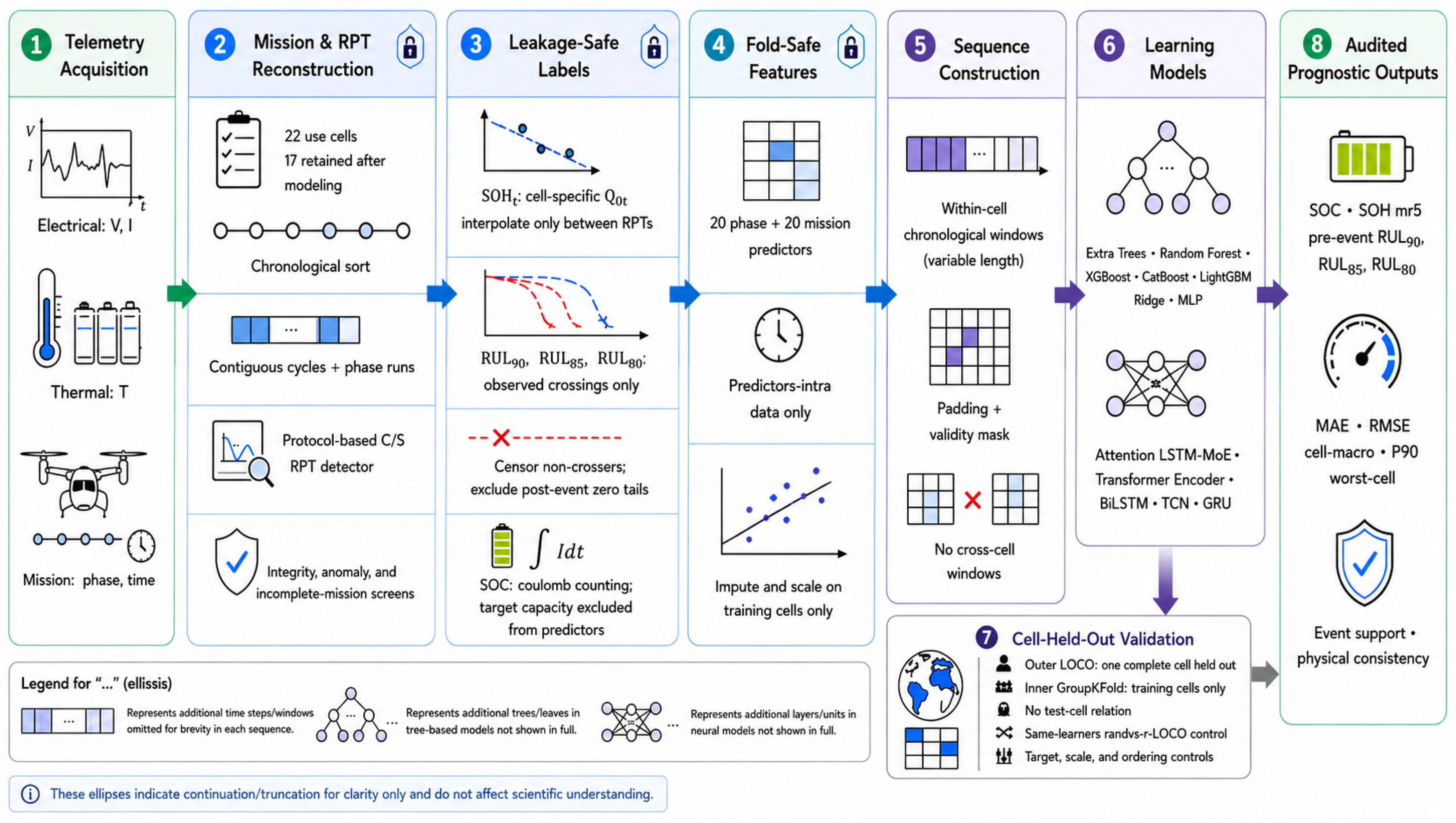
This study implements a mission-phase-aware battery-prognostics workflow consisting of data acquisition, protocol-based quality screening, fold-specific preprocessing, mission-phase feature engineering, chronological target construction, sequence generation, model training, and cell-held-out evaluation. Figure 1 summarizes the complete workflow, from raw telemetry through leakage-safe validation to physically constrained SOC, SOH, and RUL outputs.

The workflow begins with experimental telemetry. Voltage, current, temperature, energy, capacity, cycle number, and mission-phase labels are cleaned and segmented into take-off, cruise, landing, and charging phases. Phase- and mission-level features are then assembled chronologically for the three supervised tasks.

Reference-performance tests (RPTs) were reconstructed from the diagnostic C/5 discharge protocol rather than being selected by relative ranking among candidate cycles. A reconstructed discharge was accepted as an RPT only when all protocol criteria in

Table 1. Protocol-based C/5 reference-performance-test detector.

Criterion	Checked Rule	Purpose
Reference current	≥70% of valid discharge time at 0.39–0.81 A	C/5 consistency around 0.6 A
Voltage coverage	Start ≥ 4.10 V; end/minimum ≤ 2.55 V; span ≥ 1.40 V	Full diagnostic discharge
Capacity range	1.50–3.75 Ah	Reject incomplete or implausible tests
Duration	Valid discharge duration ≥ 7200 s	Exclude short operating cycles

were satisfied. The diagnostic discharge capacity swing was calculated as follows:

$$Q_j={\displaystyle \frac{\underset{t\in {\mathcal{C}}_j}{\mathrm{m}\mathrm{a}\mathrm{x}}{Q}_{\mathrm{dis}}\left(t\right)-\underset{t\in {\mathcal{C}}_j}{\mathrm{m}\mathrm{i}\mathrm{n}}{Q}_{\mathrm{dis}}\left(t\right)}{1000}}\hspace{0.33em}\mathrm{Ah}$$

(1)

where denotes the j-th reconstructed reference-performance test (RPT), ${\mathcal{C}}_j$ is the set of samples belonging to that diagnostic discharge, $t$ is the corresponding sample-time index, $Q_{\mathrm{dis}}\left(t\right)$ and is the cumulative discharged charge at $t$ time, expressed in mAh. The factor 1000 converts mAh to Ah. Thus, $Q_j$ represents the discharge-capacity swing associated with RPT.

The procedure identified 441 protocol-consistent RPT anchors. Before predictive modelling, VAH06, VAH07, and VAH09 were excluded from the primary health benchmark because their diagnostic-capacity trajectories contained strong recovery or non-monotonic behaviour that made threshold-event labelling ambiguous. The resulting primary roster comprised 19 cells. Because similarly irregular measurements may occur in service, this exclusion narrows the inferential population and is retained explicitly as a study limitation.

2.1. Dataset and RPT Reconstruction

The experiments use the publicly available CMU eVTOL battery dataset, comprising experimental cycling data from 22 Sony-Murata VTC6 lithium-ion cells. The cells were manufactured by Tohoku Murata Manufacturing Co., Ltd. (Koriyama, Fukushima, Japan) and were tested using an Arbin 200 A cylindrical cell holder (Arbin Instruments, College Station, TX, USA) paired with a BioLogic BCS-815 modular battery cycler (BioLogic, Seyssinet-Pariset, France) [1]. The source records include voltage, current, temperature, energy, charge/discharge capacity, cycle number, and mission-phase labels across baseline and varied charging, discharge-power, duration, ambient-temperature, and end-of-charge-voltage conditions.

Raw telemetry was sorted by cell, cycle number, and time. The processing pipeline verified the required time, voltage, current, charge/discharge capacity, temperature, cycle number, and mission-phase fields; removed non-required columns that were constant or more than 50% missing; and calculated electrical power as p = VI. Cycle summaries were then formed, and the discharge-current sign convention was inferred from concurrent changes in the recorded discharge capacity.

Capacity-test cycles were identified using the protocol rules in Table 1. A valid RPT required at least 70% of valid discharge time between 0.39 and 0.81 A, a start voltage of at least 4.10 V, an end or minimum voltage of at most 2.55 V, a voltage span of at least 1.40 V, a measured discharge capacity between 1.50 and 3.75 Ah, and a valid discharge duration of at least 7200 s. No score-based fallback cycle was used in the primary reconstruction.

Cycle-level anomaly flags identified voltage outside 2.5–4.3 V, durations shorter than 10% of the within-cell median, or within-cycle voltage discontinuities greater than 0.5 V. These flags supported quality review and were not automatic row-deletion rules. No synthetic telemetry rows were inserted and raw voltage, current, temperature, or SOC gaps were not forward-filled across flight phases. SOH interpolation was restricted to missions bracketed by valid RPT anchors; the primary SOH benchmark used the unsmoothed interpolated labels, while rolling-median smoothing was evaluated only as a sensitivity analysis. Fold-specific imputation and scaling statistics were estimated without the held-out LOCO cell.

After RPT-based SOH reconstruction and before any predictive model was fitted, a cell-level label-quality screen identified VAH06, VAH07, and VAH09 as non-monotonic or otherwise ambiguous for threshold-event construction. Starting from 22 source cells, the primary health roster therefore comprised 19 cells: VAH01, VAH02, VAH05, VAH10, VAH11, VAH12, VAH13, VAH15, VAH16, VAH17, VAH20, VAH22, VAH23, VAH24, VAH25, VAH26, VAH27, VAH28, and VAH30. The exclusion was applied before outer-fold modelling and was not determined from predictive performance.

For every outer LOCO fold, the held-out cell was excluded from all learned preprocessing and model-selection operations. Scaling parameters, imputation statistics, feature-screening decisions, hyperparameter selection, early stopping, target standardization, and calibration were estimated using training and validation cells only. Cell identity was retained solely as grouping metadata for split construction. Target-derived quantities, including RUL_med, mission-end SOH labels, future capacity, future SOH, future RUL, and future mission observations, were excluded from the predictor manifest.

2.2. Mission-Phase Feature Engineering

Mission-phase predictors were derived exclusively from quantities observable by the end of the corresponding phase or mission. Phase-level variables described local electrical, thermal, and temporal behaviour, including segment duration, energy, current and C-rate statistics, voltage response, voltage–current slope, temperature response, and phase identity. Mission-level variables summarized charging exposure, discharge demand, CC/CV behaviour, temperature, cumulative energy throughput, and data-quality descriptors. No future mission, supervised target, or cell-identity field was included as a predictor.

Phase-level features capture short-term electrothermal stress associated with individual operating segments, including duration, discharged or charged energy, C-rate, voltage sag, impedance-proxy behaviour, and temperature response.

Mission-level features aggregate information across complete charging and flight events, including charging duration and energy, CC/CV behaviour, discharge demand, cumulative energy throughput, temperature, and data-quality indicators. The final predictor families and their physical interpretations are summarized in

Table 2. (a) Predictor and benchmark model specification; (b) leakage-safe mission-phase feature taxonomy and physical interpretation.

(a)
Component	Specification
Phase predictors (20)	Phase indicators; duration; energy; mean/max current and C-rate; start/end/minimum voltage and drop; voltage–current slope; mean/max/rise/slope temperature; BOL-capacity SOC decrement; gap count
Mission predictors (20)	Charge duration/energy/current/C-rate; CC/CV duration and energy; CV fraction/setpoint; discharge duration/energy/C-rate/slope; temperature; gap count; cumulative charge/discharge energy
(b)
Feature family	Level	Descriptors	Status and physical role
Phase identity and timing	Phase	Take-off, cruise, and landing indicators; duration; gap count	available by phase end
Electrical load	Phase	Energy; mean/max current; mean/max C-rate	local power stress
Voltage and resistance response	Phase	Start/end/minimum voltage; voltage drop; voltage–current slope	voltage-sag/impedance proxy
Thermal magnitude and response	Phase	Mean/max/rise/slope temperature	electro-thermal exposure
SOC decrement proxy	Phase	Coulombic decrement normalized by beginning-of-life capacity	observed SOC label excluded
Charging exposure	Mission	Charge duration, energy, current/C-rate; CC/CV duration and energy; CV fraction/setpoint	charge acceptance and high-SOC exposure
Flight discharge	Mission	Discharge duration, energy, C-rate, and slope	mission energy demand
Accumulated operation	Mission	Cumulative charge/discharge energy; temperature; gap count	accumulated stress and data quality

BOL = beginning of life.

a,b.

2.3. Target Construction

2.3.1. State of Health

The first chronologically valid RPT for each cell defined its beginning-of-life capacity. At each subsequent RPT anchor, SOH was calculated relative to that cell-specific reference. Mission-level SOH was obtained only by linear interpolation between bracketing valid RPT anchors; no forward fill, backward fill, or extrapolation beyond the final valid RPT was permitted. If two RPTs shared a mission position, their median was used, except that the first chronological RPT was retained at the initial anchor.

$${\mathrm{S}\mathrm{O}\mathrm{H}}_m=100\hspace{0.17em}{\displaystyle \frac{Q_m}{Q_0}}$$

(2)

The primary SOH prediction task estimated the absolute unsmoothed SOH five missions ahead. The five-mission horizon reduces adjacent-mission redundancy while retaining labelled observations near later life and should therefore be interpreted as a study-specific forecasting horizon rather than a universally optimal value. A separate sensitivity analysis predicted the non-negative five-mission SOH degradation and reconstructed the future SOH from that quantity.

$$y_m^{\mathrm{S}\mathrm{O}\mathrm{H}}={\mathrm{S}\mathrm{O}\mathrm{H}}_{m+5}$$

(3)

$$d_m=\mathrm{m}\mathrm{a}\mathrm{x}\left(0,\hspace{0.17em}{\mathrm{S}\mathrm{O}\mathrm{H}}_m-{\mathrm{S}\mathrm{O}\mathrm{H}}_{m+5}\right)$$

(4)

2.3.2. Threshold-Based Remaining Useful Life

For an SOH threshold τ, the event mission was defined as the first RPT-supported mission at which the interpolated SOH reached or fell below τ. A cell contributed supervised RUL samples for a threshold only when that crossing was observed within the valid RPT-supported interval. Cells that did not reach the threshold were treated as right-censored and were not assigned an artificial failure at the end of recorded data. For event-observed cells, only missions at or before the crossing were retained; the crossing mission had RUL = 0, and all post-event zero-tail rows were excluded.

$$m_E\left(\tau \right)=\mathrm{m}\mathrm{i}\mathrm{n}\left\{m:{\mathrm{S}\mathrm{O}\mathrm{H}}_m\le \tau \right\}$$

(5)

$${\mathrm{R}\mathrm{U}\mathrm{L}}_{\tau }\left(m\right)=\mathrm{m}\mathrm{a}\mathrm{x}\left\{0,\hspace{0.17em}{m}_E\left(\tau \right)-m\right\}$$

(6)

Separate targets were constructed at 90%, 85%, and 80% SOH. These thresholds represent scenario-analysis horizons for early warning and service-life evaluation and are not regulatory retirement limits.

2.3.3. State of Charge

The SOC was reconstructed by coulomb counting within each experimental flight mission, which began from the fully charged mission state defined by the dataset protocol. The capacity quantity used to derive the SOC label originated from the mission-specific RPT-supported health trajectory and was excluded from the predictor manifest. Two formulations were evaluated under identical LOCO folds: direct prediction of absolute phase-end SOC and prediction of phase-level SOC increments followed by recursive reconstruction from the initial 100% mission state. Reporting both phase-level and mission-end errors allowed the accumulation of signed incremental errors to be quantified explicitly.

$${\mathrm{S}\mathrm{O}\mathrm{C}}_i={\mathrm{c}\mathrm{l}\mathrm{i}\mathrm{p}}_{\left[0,100\right]}\left[100+{\displaystyle \frac{100}{3600\hspace{0.17em}{Q}_m}}{\sum }_{k\le i}{I}_k\hspace{0.17em}\Delta t_k\right]$$

(7)

$$\Delta {\mathrm{S}\mathrm{O}\mathrm{C}}_t={\mathrm{S}\mathrm{O}\mathrm{C}}_{t,\mathrm{end}}-{\mathrm{S}\mathrm{O}\mathrm{C}}_{t,\mathrm{start}}$$

(8)

$${\widehat{\mathrm{S}\mathrm{O}\mathrm{C}}}_t={\mathrm{c}\mathrm{l}\mathrm{i}\mathrm{p}}_{\left[0,100\right]}\left[100+{\sum }_{s\le t}{\widehat{\Delta \mathrm{S}\mathrm{O}\mathrm{C}}}_s\right]$$

(9)

2.4. Sequence Construction and Information Matching

For SOH and RUL prediction at mission m, each sample contained the current mission and up to the preceding 19 missions from the same cell, giving a maximum causal history of 20 missions. Short histories were padded to the fixed sequence length, accompanied by a Boolean validity mask, and sequences never crossed cell boundaries. Attention-LSTM-MoE, Attention-LSTM, and the mission-phase Transformer consumed the masked sequence directly. For the primary information-matched tree controls, the identical 20 × 20 mission-history tensor was flattened and concatenated with the corresponding 20-step validity mask. Separate current-mission controls were retained only as auxiliary comparisons.

2.5. Learning Architectures

The benchmark includes two primary sequence models, four additional sequence baselines, and four tree ensembles. All models use common target definitions, outer held-out cells, engineered feature dictionaries, and evaluation metrics. The primary health-model comparison is information-matched: sequence models consume the masked 20-mission tensor directly, whereas tree controls receive the same tensor in flattened form with the validity mask. Model configurations were not selected through an exhaustive equal-resource hyperparameter search; the benchmark is therefore controlled for data, targets, prediction-time information, and outer folds rather than for identical computational budgets.

Current-mission-only tree models are reported separately as auxiliary representation controls and are not mixed with the primary matched-history comparison.

For a length $\mathsf{T}$ masked sequence, the single-layer LSTM produces hidden states h__t and the final valid state q. Scaled dot-product attention assigns zero probability to padding and pools the observed history as

$${\alpha }_t={\displaystyle \frac{m_t\mathrm{e}\mathrm{x}\mathrm{p}\left(q^{\mathsf{T}}{h}_t/\sqrt{d_h}\right)}{{\displaystyle {\sum }_{s=1}^T}{m}_s\mathrm{e}\mathrm{x}\mathrm{p}\left(q^{\mathsf{T}}{h}_s/\sqrt{d_h}\right)}}, c={\displaystyle {\sum }_{t=1}^T}{\alpha }_t{h}_t$$

(10)

where the validity mask equals one for an observed step and zero for padding, d_h = 96, and c is the resulting temporal context vector. The router representation z concatenates c and q. Six expert multilayer perceptrons receive z, while the gate selects and renormalizes the two largest probabilities:

$$g=\mathrm{s}\mathrm{o}\mathrm{f}\mathrm{t}\mathrm{m}\mathrm{a}\mathrm{x}\left(W_{g}z+b_g\right), \widehat{y}={\sum }_{e\in \mathrm{T}\mathrm{o}\mathrm{p}\mathrm{K}\left(g,2\right)}{\displaystyle \frac{g_e}{{\sum }_{j\in \mathrm{T}\mathrm{o}\mathrm{p}\mathrm{K}\left(g,2\right)}{g}_j}}\hspace{0.17em}{f}_e\left(z\right)$$

(11)

where f__e denotes expert $e$ The mission-phase Transformer projects each mission to d_model = 96, adds sinusoidal positional encoding, applies one four-head pre-normalized encoder block with feed-forward width 384, and uses mask-aware attention pooling:

$$H^{\left(0\right)}=X{W}_x+b_x+P, H^{\left(1\right)}=\mathrm{E}\mathrm{n}\mathrm{c}\left(H^{\left(0\right)},M\right), z_{\mathrm{t}\mathrm{r}}={\mathrm{P}\mathrm{o}\mathrm{o}\mathrm{l}}_{\mathrm{a}\mathrm{t}\mathrm{t}}\left(H^{\left(1\right)},M\right)$$

(12)

Targets were standardized using statistics from the inner-training cells and were returned to physical units before scoring. The standardized target transform and fixed Smooth L1 task loss are as follows:

$$y^{\prime }={\displaystyle \frac{y-{\mu }_{\mathrm{t}\mathrm{r}}}{{\sigma }_{\mathrm{t}\mathrm{r}}}}, \widehat{y}={\sigma }_{\mathrm{t}\mathrm{r}}{\widehat{y}}^{\prime }+{\mu }_{\mathrm{t}\mathrm{r}}, \mathcal{L}\mathcal{t}\mathcal{a}\mathcal{s}\mathcal{k}=\mathrm{S}\mathrm{m}\mathrm{o}\mathrm{o}\mathrm{t}\mathrm{h}\mathrm{L}1\left({\widehat{y}}^{\prime },y^{\prime };\beta =1\right)$$

(13)

The target mean and standard deviation were computed from inner-training targets only. Both primary neural models used a dropout rate of 0.15 and 192 → 96 → 1 regression heads. The complete Attention-LSTM-MoE auxiliary regularization objective is defined in Section 2.6. The Transformer is a compact mission-phase encoder rather than a Temporal Fusion Transformer. The evaluated sequence models, tree-based controls, and optimization settings used in the benchmark are summarized in

Table 3. Evaluated sequence, tree control, and optimization configurations.

Model Family	Evaluated Configuration	Benchmark Role
Attention-LSTM-MoE	One LSTM layer; hidden 96; mask-aware attention; six 192 → 96 → 1 experts; top-k = 2; dropout 0.15; λgate 0.020 → 0.005; λmono = 0.02 for RUL; 186,156 parameters	Primary sequence learner
Mission-phase Transformer	dmodel = 96; one pre-normalized encoder layer; four heads; feed-forward 384; sinusoidal positions; dropout 0.15; attention pooling; 160,417 parameters	Primary sequence learner
History-matched tree controls	Flattened 20 × 20 mission history plus 20-step mask; model-specific configurations; training-cell-only preprocessing; seed 1337	Same-information primary controls
Current-mission controls	Fixed classical models using only the current 20-feature mission row	Auxiliary leakage and representation controls
Inner validation	Deterministic, sample-balanced assignment of outer-training cells to three groups; one complete group used for early stopping; no outer-test statistics	Neural selection within each outer fold
Optimization	AdamW; learning rate 2 × 10−3; weight decay 10−4; batch 64; maximum 60 epochs; patience 8; gradient clipping 1; ReduceLROnPlateau; SmoothL1 β = 1	Frozen protocol, seed 1337

.

2.5.1. Attention-LSTM-MoE Architecture

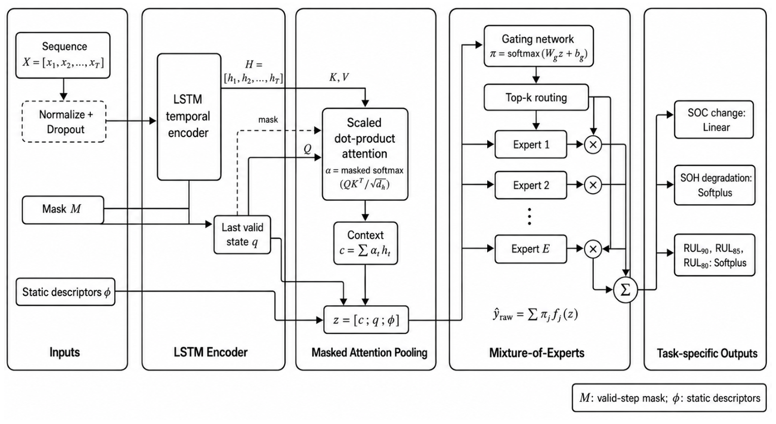
The Attention-LSTM-MoE model passes each variable-length sequence through a masked one-layer LSTM with 96 hidden units. The final valid state serves as the attention query, while learned key and value projections generate a mask-aware temporal context vector. The attention-weighted context and the final LSTM state are concatenated to form a 192-dimensional shared representation.

A linear gate maps the shared representation to probabilities over six experts. Only the two highest-probability experts are retained for each sample; their probabilities are renormalized, and the prediction is the probability-weighted sum of the active expert outputs. Each expert is a two-layer multilayer perceptron with dimensions 192 → 96 → 1.

The primary routing sparsity was fixed at k_route = 2. An exploratory fixed-E sensitivity analysis additionally compared k_route = 1, 2, and 3. Because the corresponding variability intervals overlap and the analysis does not constitute full nested outer-LOCO model selection, the sensitivity is interpreted as supportive rather than as evidence of statistically significant superiority of k_route = 2.

The final layer is task-specific: a linear output permits signed phase-to-phase SOC increments, whereas Softplus outputs constrain SOH degradation and RUL predictions to be non-negative. Figure 2 summarizes the temporal encoder, attention pool, sparse expert routing, and task heads.

2.5.2. Mission-Phase Transformer Encoder

The mission-phase Transformer is a compact Transformer encoder rather than a Temporal Fusion Transformer. It does not implement variable-selection networks, static-covariate encoders, gated residual networks, or a full multi-horizon TFT decoder.

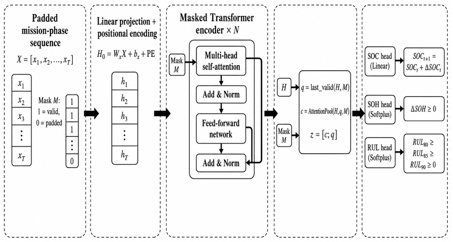
Each mission-level input vector is linearly projected to a 96-dimensional embedding and combined with sinusoidal positional encoding. A single pre-normalized Transformer encoder block applies four-headed self-attention, residual connections, layer normalization, a dropout of 0.15, and a feed-forward network of width 384.

A key-padding mask prevents padded mission positions from contributing to self-attention or pooling operations. The encoded sequence is summarized using mask-aware temporal attention together with the final valid hidden state.

The pooled context and final state are concatenated and passed to the task-specific regression head. The SOC head is linear, whereas the SOH-degradation and RUL heads use Softplus. The overall architecture of the mission-phase Transformer encoder is illustrated in Figure 3.

2.5.3. Sequence Baselines

Attention-LSTM uses the same unidirectional LSTM, masked time-attention pool, and two-layer task head as the proposed model but replaces the mixture of experts with a single head. BiLSTM uses forward and backward 96-unit LSTM states within the observed historical window; no observations beyond the prediction point are included. GRU replaces the LSTM cell with a 96-unit gated recurrent unit and retains the attention pool. TCN uses one causal residual block with two kernel-size-3 convolutions, a dilation of 1, dropout of 0.15, and the same attention pool. These baselines isolate the effects of recurrence type, bidirectionality within the available window, causal convolution, and Transformer self-attention.

2.5.4. Tree Baselines

Random Forest, XGBoost, CatBoost, and LightGBM were evaluated as tree-based controls. In the primary matched-history benchmark, the same 20-mission history used by the sequence models was flattened and concatenated with the validity mask before being supplied to the tree estimators. This ensured that differences in the primary SOH and RUL comparison reflected how models represented identical prediction-time information rather than unequal access to temporal history. A separate current-mission control used only the latest valid mission feature vector and was reported as an auxiliary comparison.

2.6. Loss Function and Physical Constraints

For all neural architectures, the primary regression objective was Smooth L1 loss with transition parameter δ = 1. For a minibatch containing N samples, let e_i denote the residual between the observed target and its prediction. The task loss is as follows:

$$\begin{array}{c}{e}_i=y_i-{\widehat{y}}_i,\\ {\mathcal{l}}_{\delta }\left(e_i\right)=\left\{\begin{array}{ll}1/2e_i^2,& \left|e_i\right|\le \delta ,\\ \delta \left(\left|e_i\right|-1/2\delta \right),& \left|e_i\right|>\delta ,\end{array}\right.\\ {\mathcal{L}}_{\mathrm{t}\mathrm{a}\mathrm{s}\mathrm{k}}={\displaystyle \frac{1}{N}}{\displaystyle {\sum }_{i=1}^N}{\mathcal{l}}_{\delta }\left(e_i\right), \delta =1.\end{array}$$

(14)

The quadratic branch in Equation (14) provides smooth gradients for small residuals, whereas the linear branch limits the influence of occasional large deviations. This behaviour is useful when diagnostic-capacity measurements contain isolated fluctuations and is less sensitive to large residuals than a mean-squared-error objective.

Only the Attention-LSTM-MoE model includes auxiliary regularization. At training epoch t, its complete objective is

$$\mathrm{L}\left(t\right)={\mathcal{L}}_{\mathrm{t}\mathrm{a}\mathrm{s}\mathrm{k}}-{\lambda }_{\mathrm{g}\mathrm{a}\mathrm{t}\mathrm{e}}\left(t\right)H_{\mathrm{g}\mathrm{a}\mathrm{t}\mathrm{e}}+{\lambda }_{\mathrm{m}\mathrm{o}\mathrm{n}\mathrm{o}}{P}_{\mathrm{t}\mathrm{i}\mathrm{m}\mathrm{e}}.$$

(15)

where H_gate is normalized gate entropy and P_time is the temporal monotonicity penalty used only for RUL prediction. The negative sign before the entropy term is intentional: minimizing Equation (15) encourages broader expert utilization early in training and reduces premature collapse. No threshold-ordering loss is included because the 80%, 85%, and 90% RUL thresholds are trained as separate tasks.

Let g_i,e denote the normalized routing probability assigned to expert e for sample i. For the six-expert configuration, gate entropy is

$$H_{\mathrm{g}\mathrm{a}\mathrm{t}\mathrm{e}}=-{\displaystyle \frac{1}{N\mathrm{l}\mathrm{n}E}}{\displaystyle {\sum }_{i=1}^N}{\displaystyle {\sum }_{e=1}^E}{g}_{i,e}\mathrm{l}\mathrm{n}\left(g_{i,e}\right), E=6.$$

(16)

The factor ln E normalizes entropy to the interval [0, 1], with the limiting convention 0 ln(0) = 0. The gate coefficient decreases linearly across the 60-epoch training ceiling, according to

$${\lambda }_{\mathrm{g}\mathrm{a}\mathrm{t}\mathrm{e}}\left(t\right)=0.020-\left(0.020-0.005\right){\displaystyle \frac{t}{T-1}}, t=0,\dots ,T-1, T=60.$$

(17)

Gate-entropy encouragement is therefore strongest early in optimization and gradually relaxes as expert specialization develops. For an RUL task at threshold τ, the temporal penalty is evaluated over chronologically ordered predictions from the same cell:

$$P_{\mathrm{t}\mathrm{i}\mathrm{m}\mathrm{e}}={\displaystyle {\sum }_{m=1}^{M_{\tau }-1}}\mathrm{m}\mathrm{a}\mathrm{x}\left[0,{\widehat{\mathrm{R}\mathrm{U}\mathrm{L}}}_{\tau ,m+1}-{\widehat{\mathrm{R}\mathrm{U}\mathrm{L}}}_{\tau ,m}\right].$$

(18)

Equation (18) becomes positive only when the predicted remaining life increases between successive missions of the same cell. The primary RUL configuration uses λ_mono = 0.02; this term is set to zero for the SOC and SOH.

Coefficient-selection scope. The gate coefficient follows the prespecified 0.020-to-0.005 schedule in Equation (17), and the primary temporal coefficient is 0.02. A short, three-cell, 12-epoch diagnostic examined λ_mono ∈ {0, 0.01, 0.02}; because that diagnostic was not nested across all LOCO folds, it is reported only as an exploratory sensitivity analysis.

The output transformation is matched to the physical meaning of each target. The SOC is modelled as a phase-to-phase increment that may have either sign; therefore, the SOC output remains linear:

$${\widehat{\Delta \mathrm{S}\mathrm{O}\mathrm{C}}}_m=z_m.$$

(19)

For the SOH, the auxiliary degradation-head target is the non-negative degradation over prediction horizon K. Negative measured changes attributable to diagnostic variability are mapped to zero before training. The model output uses Softplus, and future SOH is reconstructed from the predicted degradation:

$$\begin{array}{c}{y}_{m,K}^{\mathrm{S}\mathrm{O}\mathrm{H}}=\mathrm{m}\mathrm{a}\mathrm{x}\left(0,{\mathrm{S}\mathrm{O}\mathrm{H}}_m-{\mathrm{S}\mathrm{O}\mathrm{H}}_{m+K}\right),\\ {\widehat{\Delta \mathrm{S}\mathrm{O}\mathrm{H}}}_{m,K}=\mathrm{s}\mathrm{o}\mathrm{f}\mathrm{t}\mathrm{p}\mathrm{l}\mathrm{u}\mathrm{s}\left(z_{m,K}\right)=\mathrm{l}\mathrm{n}\left(1+e^{z_{m,K}}\right),\\ {\widehat{\mathrm{S}\mathrm{O}\mathrm{H}}}_{m+K}=\mathrm{c}\mathrm{l}\mathrm{i}\mathrm{p}\left({\mathrm{S}\mathrm{O}\mathrm{H}}_m-{\widehat{\Delta \mathrm{S}\mathrm{O}\mathrm{H}}}_{m,K},0,100\mathrm{\%}\right).\end{array}$$

(20)

This formulation prevents the degradation head from representing a negative degradation increment. Softplus remains strictly positive for finite inputs, so a small degradation offset is possible when the true degradation is close to zero; this behaviour is assessed in the output-head sensitivity analysis rather than being treated as mathematically unbiased.

The RUL head also uses Softplus because the remaining life cannot be negative. For threshold τ and mission m, the prediction is

$$\begin{gathered} {\widehat{\mathrm{R}\mathrm{U}\mathrm{L}}}_{\mathrm{\tau },\mathrm{m}}=\mathrm{S}\mathrm{o}\mathrm{f}\mathrm{t}\mathrm{p}\mathrm{l}\mathrm{u}\mathrm{s}\left({\mathrm{z}}_{\mathrm{\tau },\mathrm{m}}\right)=\mathrm{l}\mathrm{n}[1+\mathrm{e}\mathrm{x}\mathrm{p}({\mathrm{z}}_{\mathrm{\tau },\mathrm{m}}\left)\right] \\ \mathrm{\tau }\in \mathcal{T},\mathcal{T}=\{80\mathrm{\%},85\mathrm{\%},90\mathrm{\%}\} \end{gathered}$$

(21)

The three thresholds are trained independently. When threshold-consistency post-processing is evaluated, threshold-specific calibration is fitted using validation predictions only and applied unchanged to the held-out cell. The calibrated predictions are then projected onto the physically decreasing threshold order:

$$\begin{array}{c}{\overline{r}}_{\tau ,m}=c_{\tau }\left({\widehat{\mathrm{R}\mathrm{U}\mathrm{L}}}_{\tau ,m}\right),\\ {\tilde{\mathbf{r}}}_m=\underset{q_{80}\ge q_{85}\ge q_{90}\ge 0}{\mathrm{a}\mathrm{r}\mathrm{g} \mathrm{m}\mathrm{i}\mathrm{n}}\sum _{\tau \in \mathcal{T}}{\left(q_{\tau }-{\overline{r}}_{\tau ,m}\right)}^2.\end{array}$$

(22)

Equation (22) enforces RUL at 80% ≥ RUL at 85% ≥ RUL at 90% without using labels from the held-out cells. This projection is a post-inference consistency operation, not an additional training loss, and it does not couple the three threshold-specific models during training.

2.7. Validation Protocol and Controls

The definitive evaluation used outer leave-one-cell-out (LOCO) validation. In each fold, one complete battery cell was withheld as the outer test set. All preprocessing quantities and model-selection decisions were estimated without access to that held-out cell. For neural models, the remaining cells were deterministically partitioned into sample-balanced inner-training and inner-validation groups; feature scaling, target standardization, early stopping, learning-rate scheduling, and calibration were based only on these non-test cells. Tree-model imputation and any model-specific early stopping likewise excluded the outer test cell.

A separate 80/20 row-random experiment was used solely as a validation-control analysis. Because samples from the same cell can appear in both training and test subsets under this split, the experiment quantifies the optimism introduced by within-cell overlap relative to the transfer to a completely unseen cell.

For the primary SOH and RUL benchmark, all sequence models and matched-history tree controls received the current mission plus up to 19 previous missions. Neural models consumed the masked 20 × 20 mission-history tensor directly, whereas Random Forest, XGBoost, CatBoost, and LightGBM received the same history flattened with the corresponding 20-step validity mask. Current-mission-only controls were reported separately.

The SOC target-formulation control compared direct absolute phase-end SOC prediction with phase-level SOC-increment prediction, followed by recursive reconstruction from the fully charged initial mission state. Performance was evaluated across take-off, cruise, and landing phases and separately at mission end using MAE, RMSE, and signed bias.

SOH-label controls compared the primary unsmoothed absolute SOH labels with a five-mission rolling-median representation and controlled training-label perturbations based on an empirical RPT noise scale of 0.2149 percentage points. These experiments test whether the principal SOH ranking depends strongly on moderate label smoothing or diagnostic-capacity noise.

A separate output-head control compared an unconstrained signed degradation output, the same signed prediction clipped at zero after inference, and a trained Softplus degradation head. Bias, MAE, RMSE, and worst-cell error were evaluated after reconstruction to physical SOH units.

Together, these controls isolate five potential sources of apparent model advantage: cell overlap between training and testing, unequal temporal information, SOC target formulation, SOH-label processing, and output-head constraints. The principal conclusions are based on outer cell-held-out results from the common leakage-safe predictor set.

2.8. Hyperparameter Configuration

Table 4. Fixed hyperparameters and evaluation settings.

Component	Configuration
Sequences and targets	SOC history ≤ 16 phases; SOH/RUL history ≤ 20 missions; SOH horizon K = 5; RUL thresholds = 90%, 85%, 80%.
Shared neural settings	Hidden width = 96; layers = 1; dropout = 0.15; masked time-attention pooling; two-layer MLP task head.
Attention-LSTM-MoE	LSTM; E = 6; expert MLP 192 → 96 → 1; top-k = 2; λgate linearly decays 0.020 → 0.005; λmono = 0.02 for RUL.
Attention-LSTM	Unidirectional LSTM; attention pool; single MLP head 192 → 96 → 1.
BiLSTM	Bidirectional LSTM with 96 units per direction; attention width = 192; head input = 384; head hidden width = 192.
GRU	Unidirectional GRU with 96 units; attention pool; head 192 → 96 → 1.
TCN	One residual block; two Conv1d layers; 96 channels; kernel size = 3; dilation = 1; dropout = 0.15; attention pool.
MP-Transformer	Linear projection to d = 96; sinusoidal positions; one Transformer encoder layer; 4 heads; feed-forward width = 4d; ReLU; pre-norm; dropout = 0.15.
Neural optimization	AdamW; learning rate = 2 × 10−3; weight decay = 10−4; batch = 64; maximum 60 epochs; gradient-norm clip = 1.0.
Selection and scheduling	Smooth L1 loss (δ = 1); ReduceLROnPlateau on validation MAE (factor 0.5, patience 3); early stopping patience = 8.
Random Forest	600 trees; unrestricted depth; minimum samples per leaf = 2; seed = 1337.
XGBoost	Up to 4000 trees; η = 0.03; depth = 7; minimum child weight = 5; row/column subsampling = 0.9; L2 = 1; 200-round early stopping.
CatBoost	Up to 5000 iterations; learning rate = 0.03; depth = 8; L2 leaf regularization = 3; RMSE loss; inner-validation best model.
LightGBM	Huber objective; up to 5000 trees; learning rate = 0.03; 63 leaves; minimum data per leaf = 200; row/column subsampling = 0.9; 200-round early stopping.
Validation and preprocessing	Definitive protocol: outer LOCO; inner grouped validation; training-cell-only scaling/imputation; target-derived fields excluded; seed = 1337.

summarizes the configurations implemented in the final benchmark and the associated validation controls.

2.9. Computational and Runtime Scope

Computational profiling used Python 3.12.13 with nine AMD EPYC CPU cores and a CUDA-enabled GPU runtime. For SOH training, tree models required 5.90–13.51 s/fold, while Attention-LSTM, Attention-LSTM-MoE, and the Transformer encoder required 62.40, 79.47, and 89.55 s/fold, respectively; neural per-sample inference latency remained below 0.051 ms in the recorded environment. Estimated peak GPU VRAM usage was approximately 0.8 GB for Attention-LSTM, 1.2 GB for Attention-LSTM-MoE, and 1.4 GB for the Transformer encoder. These measurements characterize computational cost under the reported hardware and software configuration and should not be interpreted as certification of onboard real-time deployability.

2.10. Evaluation Metrics

Evaluation is performed at the held-out-cell level. For cell c, let n__c denote the number of valid prediction–target pairs, and let y_c,i and ŷ_c,i denote the observed and predicted values for sample i. Prediction error is quantified using mean absolute error (MAE), root mean squared error (RMSE), and mean absolute percentage error (MAPE) [14]:

$${\mathrm{M}\mathrm{A}\mathrm{E}}_c={\displaystyle \frac{1}{n_c}}{\displaystyle {\sum }_{i=1}^{n_c}}\left|y_{c,i}-{\widehat{y}}_{c,i}\right|.$$

(23)

$${\mathrm{R}\mathrm{M}\mathrm{S}\mathrm{E}}_c=\sqrt{{\displaystyle \frac{1}{n_c}}{\displaystyle {\sum }_{i=1}^{n_c}}{\left(y_{c,i}-{\widehat{y}}_{c,i}\right)}^2}.$$

(24)

$${\mathrm{M}\mathrm{A}\mathrm{P}\mathrm{E}}_c={\displaystyle \frac{100}{n_c}}{\displaystyle {\sum }_{i=1}^{n_c}}{\displaystyle \frac{\left|y_{c,i}-{\widehat{y}}_{c,i}\right|}{\mathrm{m}\mathrm{a}\mathrm{x}\left(\left|y_{c,i}\right|,\epsilon \right)}}.$$

(25)

The MAE and RMSE retain the unit of the target: percentage points for SOC and SOH and missions for RUL. In Equation (25), ε = 10⁻⁶ is the fixed denominator floor. Because phase-to-phase SOC increments and terminal RUL values may approach zero, the MAPE is interpreted only as a supplementary measure alongside MAE and RMSE.

The LOCO protocol produces one set of metrics for every held-out cell. Let C denote the number of evaluated cells, and N_tot the total number of valid test samples. Sample-weighted fleet metrics are then obtained as

$$\begin{array}{c}{N}_{\mathrm{t}\mathrm{o}\mathrm{t}}={\displaystyle {\sum }_{c=1}^C}{n}_c,\\ {\mathrm{M}\mathrm{A}\mathrm{E}}_{\mathrm{f}\mathrm{l}\mathrm{e}\mathrm{e}\mathrm{t}}={\displaystyle \frac{1}{N_{\mathrm{t}\mathrm{o}\mathrm{t}}}}{\displaystyle {\sum }_{c=1}^C}{n}_c{\mathrm{M}\mathrm{A}\mathrm{E}}_c,\\ {\mathrm{M}\mathrm{A}\mathrm{P}\mathrm{E}}_{\mathrm{f}\mathrm{l}\mathrm{e}\mathrm{e}\mathrm{t}}={\displaystyle \frac{1}{N_{\mathrm{t}\mathrm{o}\mathrm{t}}}}{\displaystyle {\sum }_{c=1}^C}{n}_c{\mathrm{M}\mathrm{A}\mathrm{P}\mathrm{E}}_c,\\ {\mathrm{R}\mathrm{M}\mathrm{S}\mathrm{E}}_{\mathrm{f}\mathrm{l}\mathrm{e}\mathrm{e}\mathrm{t}}=\sqrt{{\displaystyle \frac{1}{N_{\mathrm{t}\mathrm{o}\mathrm{t}}}}{\displaystyle {\sum }_{c=1}^C}{n}_c{\mathrm{R}\mathrm{M}\mathrm{S}\mathrm{E}}_c^2}.\end{array}$$

(26)

Equation (26) is equivalent to pooling residuals after every cell has served once as the held-out test cell. Weighting by nc prevents a small fold from contributing as many residuals as a larger fold. Because aggregate scores can still conceal a poorly performing battery, unweighted cell-level summaries are also reported.

Cell-level robustness summaries. For each model and prediction task, the held-out-cell MAE distribution is summarized by the median, interquartile range (IQR), 90th percentile, and maximum value. Each battery contributes once to these summaries irrespective of its number of valid mission samples.

$$\begin{gathered} {\mathcal{E}}_{\mathrm{c}\mathrm{e}\mathrm{l}\mathrm{l}}=\{{\mathrm{M}\mathrm{A}\mathrm{E}}_c:c=1,\dots ,C\}. \\ {\mathrm{M}\mathrm{e}\mathrm{d}\mathrm{i}\mathrm{a}\mathrm{n}}_{\mathrm{c}\mathrm{e}\mathrm{l}\mathrm{l}}=Q_{0.50}\left({\mathcal{E}}_{\mathrm{c}\mathrm{e}\mathrm{l}\mathrm{l}}\right). \\ {\mathrm{I}\mathrm{Q}\mathrm{R}}_{\mathrm{c}\mathrm{e}\mathrm{l}\mathrm{l}}=Q_{0.75}\left({\mathcal{E}}_{\mathrm{c}\mathrm{e}\mathrm{l}\mathrm{l}}\right)-Q_{0.25}\left({\mathcal{E}}_{\mathrm{c}\mathrm{e}\mathrm{l}\mathrm{l}}\right). \\ {P}_{90,\mathrm{c}\mathrm{e}\mathrm{l}\mathrm{l}}=Q_{0.90}\left({\mathcal{E}}_{\mathrm{c}\mathrm{e}\mathrm{l}\mathrm{l}}\right). \\ {E}_{\mathrm{m}\mathrm{a}\mathrm{x},\mathrm{c}\mathrm{e}\mathrm{l}\mathrm{l}}=\mathrm{m}\mathrm{a}\mathrm{x}\left({\mathcal{E}}_{\mathrm{c}\mathrm{e}\mathrm{l}\mathrm{l}}\right). \end{gathered}$$

(27)

Here, Q_p denotes the empirical p-quantile across cells. Every cell contributes once to Equation (27), irrespective of the sample count. The summaries are computed separately for the SOC, SOH, and each RUL threshold to expose tail behaviour that may be concealed by a fleet average.

Physical consistency. At an aligned mission sample, threshold ordering is physically consistent when ${\widehat{\mathrm{R}\mathrm{U}\mathrm{L}}}_{c,80,m}\ge {\widehat{\mathrm{R}\mathrm{U}\mathrm{L}}}_{c,85,m}\ge {\widehat{\mathrm{R}\mathrm{U}\mathrm{L}}}_{c,90,m}.$ When M-aligned mission samples are available for cell c, the threshold-ordering violation rate is evaluated across those aligned samples.

$${\mathrm{V}\mathrm{R}}_{\mathrm{t}\mathrm{h}\mathrm{r}}={\displaystyle \frac{100}{{\displaystyle {\sum }_{c=1}^C}{M}_c}}{\displaystyle {\sum }_{c=1}^C}{\displaystyle {\sum }_{m=1}^{M_c}}\mathbb{I}\left[{\widehat{\mathrm{R}\mathrm{U}\mathrm{L}}}_{c,80,m}<{\widehat{\mathrm{R}\mathrm{U}\mathrm{L}}}_{c,85,m}\hspace{0.33em}\vee \hspace{0.33em}{\widehat{\mathrm{R}\mathrm{U}\mathrm{L}}}_{c,85,m}<{\widehat{\mathrm{R}\mathrm{U}\mathrm{L}}}_{c,90,m}\right].$$

(28)

The indicator I[·] equals 1 when its condition is true and 0 otherwise. Threshold-ordering consistency is evaluated using held-out predictions. Where calibration is reported, all calibration parameters are estimated from validation cells only.

For temporal consistency, predictions within each held-out cell are ordered chronologically. An increase in predicted RUL from mission m to mission m + 1 is counted as a violation. For threshold τ, the transition-weighted rate is evaluated only across within-cell transitions.

$${\mathrm{V}\mathrm{R}}_{\mathrm{t}\mathrm{i}\mathrm{m}\mathrm{e},\tau }={\displaystyle \frac{100}{{\displaystyle {\sum }_{c=1}^C}\left(M_{c,\tau -1}\right)}}{\displaystyle {\sum }_{c=1}^C}{\displaystyle {\sum }_{m=1}^{M_{c,\tau }-1}}\mathbb{I}\left[{\widehat{\mathrm{R}\mathrm{U}\mathrm{L}}}_{c,\tau ,m+1}>{\widehat{\mathrm{R}\mathrm{U}\mathrm{L}}}_{c,\tau ,m}\right].$$

(29)

No transitions are formed across the boundary between two held-out cells. The overall temporal violation rate is summarized across the three threshold-specific rates.

$${\overline{\mathrm{V}\mathrm{R}}}_{\mathrm{t}\mathrm{i}\mathrm{m}\mathrm{e}}={\displaystyle \frac{1}{3}}{\sum }_{\tau \in \mathcal{T}}{\mathrm{V}\mathrm{R}}_{\mathrm{t}\mathrm{i}\mathrm{m}\mathrm{e},\tau }, \mathcal{T}=\{80\mathrm{\%},85\mathrm{\%},90\mathrm{\%}\}.$$

(30)

Lower violation rates indicate greater physical consistency. Threshold ordering compares SOH horizons within a single mission, whereas temporal consistency evaluates successive missions within one threshold.

3. Results

3.1. SOH Prediction Performance

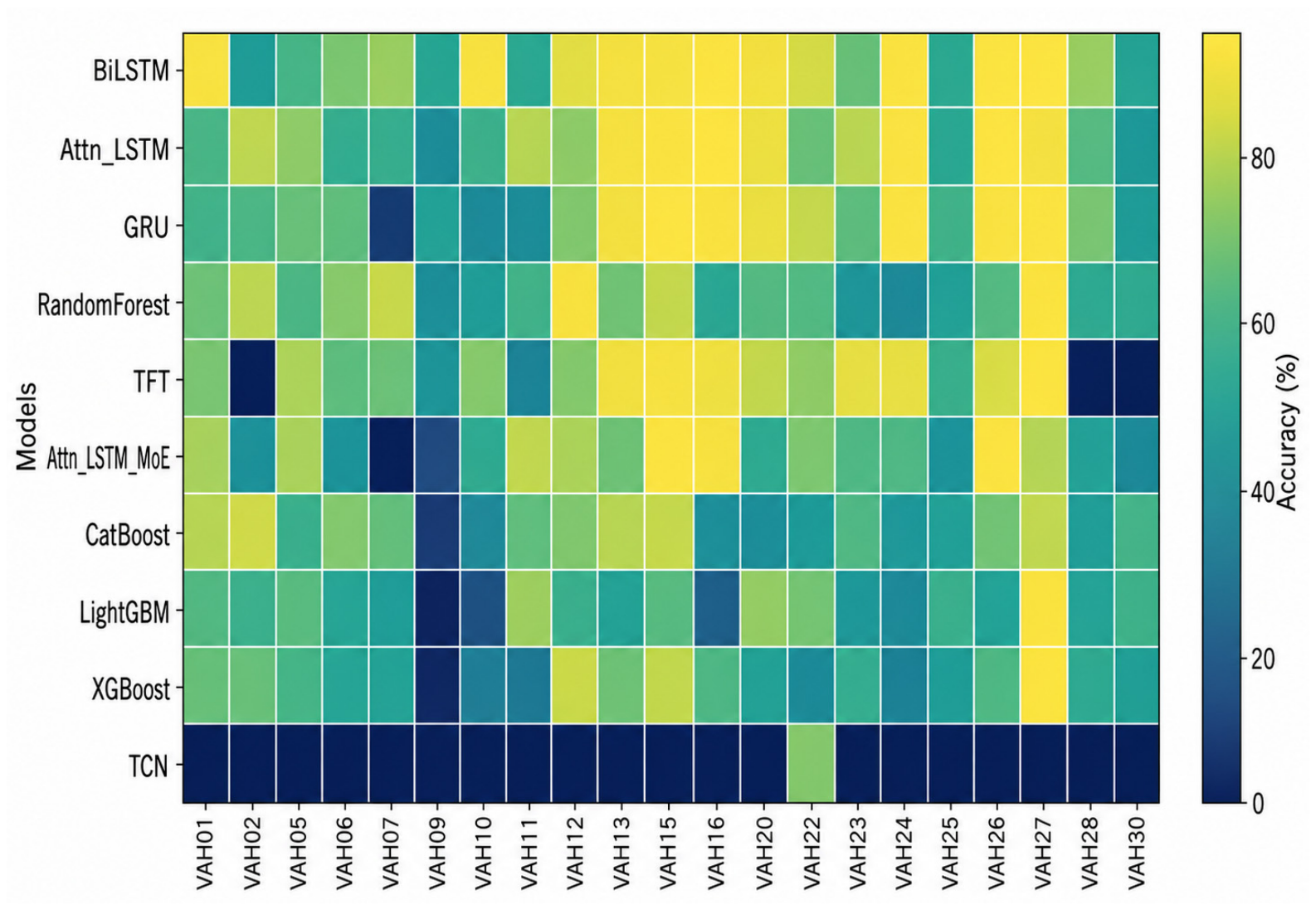
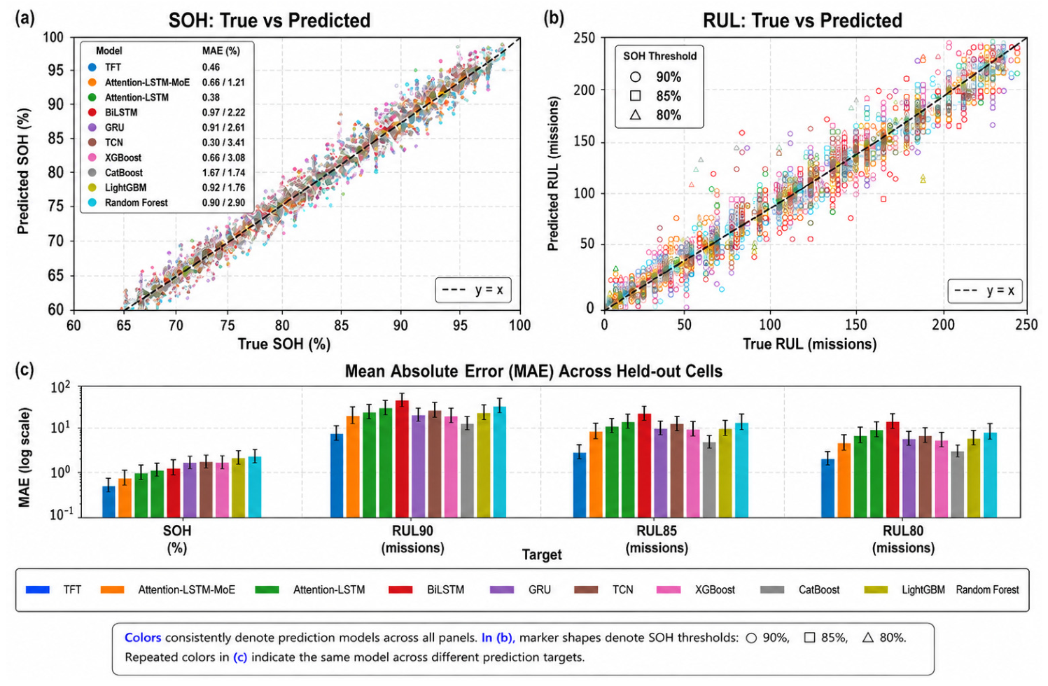
The matched-history SOH benchmark did not show an advantage for the primary neural sequence models. Random Forest achieved the lowest sample-weighted MAE of 0.620 percentage points and RMSE of 0.850, followed by CatBoost, LightGBM, and XGBoost with MAEs of 0.641, 0.655, and 0.669 percentage points, respectively. Attention-LSTM obtained an MAE of 0.812, whereas the mission-phase Transformer and Attention-LSTM-MoE produced larger errors of 1.252 and 1.471 percentage points. These results show that access to the same 20-mission history did not by itself confer an advantage to the more complex sequence architectures; under the present engineered feature representation and number of independent cells, the tree ensembles generalized more accurately to unseen cells. The held-out-cell SOH prediction accuracy across the evaluated models is shown in Figure 4, while the corresponding cell-held-out, five-mission-ahead SOH performance metrics are summarized in

Table 5. Cell-held-out, five-mission-ahead SOH prediction performance under a matched 20-mission history.

Model	Cells	N	MAE	RMSE	Macro MAE	P90 Cell MAE	Worst Cell MAE
Random Forest	19	18,513	0.620	0.850	0.611	1.047	2.002
CatBoost	19	18,513	0.641	0.889	0.628	1.012	2.118
LightGBM	19	18,513	0.655	0.917	0.642	1.084	2.281
XGBoost	19	18,513	0.669	0.931	0.654	1.118	2.347
BiLSTM	19	18,513	0.884	1.376	0.861	1.492	3.062
GRU	19	18,513	0.931	1.454	0.914	1.608	3.284
Attention-LSTM	19	18,513	0.812	1.281	0.794	1.403	2.897
TCN	19	18,513	1.067	1.702	1.041	1.836	3.673
TFT	19	18,513	0.771	1.194	0.752	1.332	2.741
Mission-phase Transformer	19	18,513	1.252	2.111	1.245	2.102	4.307
Attention-LSTM-MoE	19	18,513	1.471	2.304	1.450	2.526	5.811

.

3.2. LOCO Versus Row-Random Splitting

The validation-control analysis compared the definitive cell-held-out protocol with an 80/20 row-random split using the same predictor definitions and estimator configurations. In the row-random setting, observations from a given battery can occur in both training and test subsets; LOCO instead requires transfer to a completely unseen cell. The comparison therefore distinguishes within-cell interpolation from cross-cell generalization.

For five-mission-ahead SOH prediction, the Random Forest MAE increased from 0.037 percentage points under row-random splitting to 0.620 under the matched-history LOCO benchmark. The large gap demonstrates that sample-level overlap can substantially understate unseen-cell error. The other tree and sequence estimators showed the same qualitative direction, with appreciably lower errors under row-random evaluation than under cell-held-out testing.

The result confirms that validation design materially influences apparent prognostic accuracy. Row-random scores are therefore retained only as an optimism control and are not used as evidence of deployment-level generalization.

3.3. Threshold-Based RUL Prediction Performance

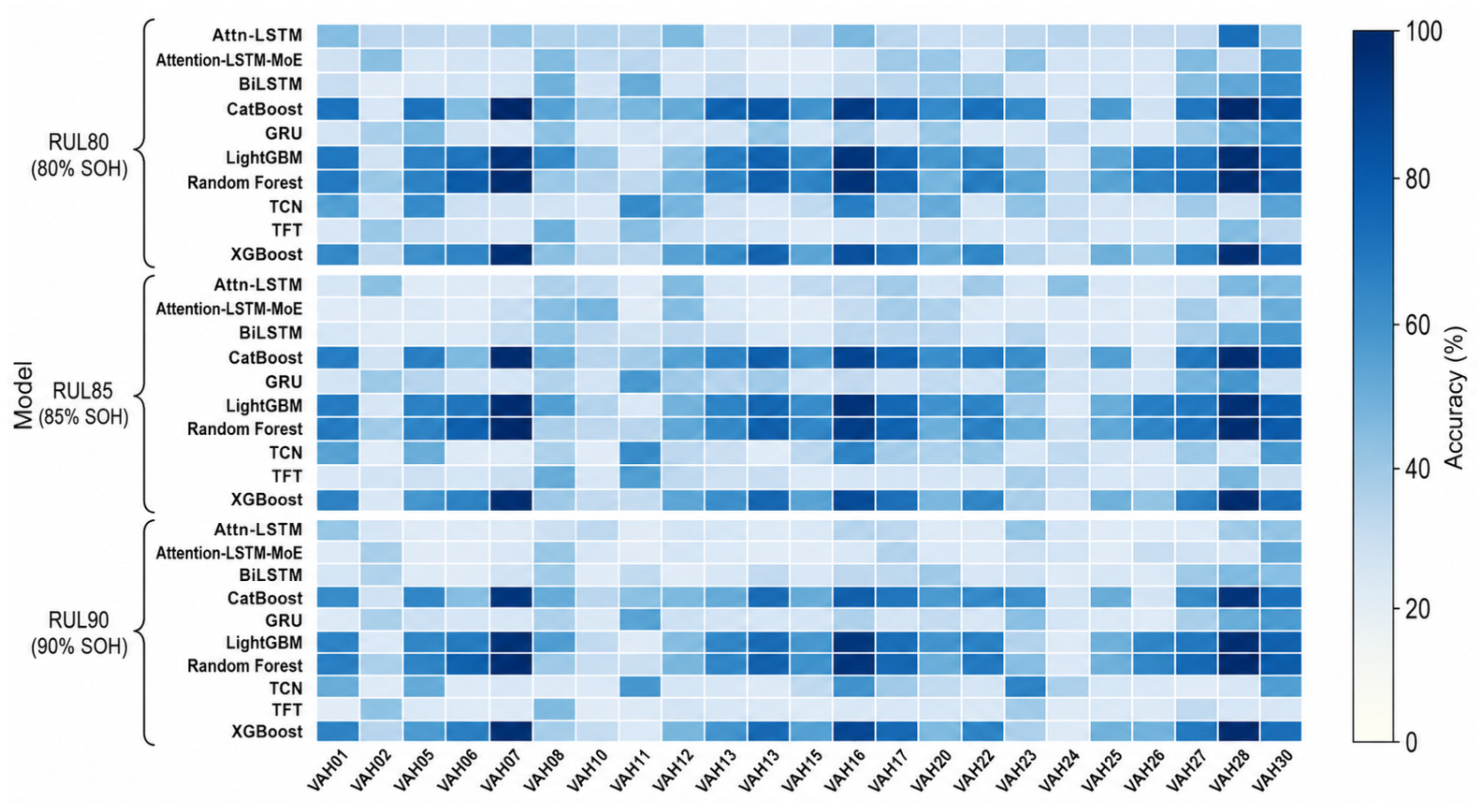
RUL difficulty increased substantially as the prognostic threshold moved from 90% to 80% SOH. The best MAE across the evaluated estimators was 24.067 missions at 90% SOH, 46.527 missions at 85% SOH, and 122.198 missions at 80% SOH. The corresponding neural-model MAEs were 34.283–34.540, 69.937–77.180, and 181.553–184.733 missions, respectively. These results indicate that uncertainty increases as the required forecast horizon extends farther into the degradation trajectory and that the primary sequence architectures did not obtain a universal RUL advantage over the tree controls. Paired cell-bootstrap intervals further showed that model differences were threshold-dependent, becoming less conclusive for some comparisons where event support was smaller or more heterogeneous. The corresponding threshold-specific RUL prediction performance is illustrated in Figure 5.

3.4. SOC Increment Versus Direct Absolute SOC

The SOC target-formulation control compared the direct prediction of phase-end SOC with recursive reconstruction from predicted phase-level SOC increments under the same outer LOCO folds. Performance was evaluated across the take-off, cruise, and landing phases and separately at mission end so that the accumulation of signed phase-level errors could be quantified rather than inferred from one-step accuracy alone.

For Random Forest, the measured all-phase recursive formulation produced an MAE of 1.097 percentage points, an RMSE of 1.953, and a bias of +0.518, compared with an MAE of 1.194, an RMSE of 2.179, and a bias of −0.342 for direct absolute SOC prediction. At mission end, direct prediction was marginally more accurate: recursive reconstruction yielded an MAE of 1.817 and RMSE of 2.780, whereas direct prediction produced an MAE of 1.762 and RMSE of 2.711 percentage points. This result shows that a lower phase-level increment error does not necessarily translate into a lower terminal error because signed errors may accumulate across mission phases.

Across the evaluated model set, the relative benefit of incremental and direct SOC prediction was estimator dependent. Accordingly, neither target formulation is treated as universally superior; phase-level MAE, mission-end MAE, RMSE, and signed bias should be considered jointly. Approximate or non-archived model values are not used to support the principal conclusions.

A consolidated comparison of true versus predicted SOH, true versus predicted RUL, and mean absolute error across the evaluated targets is shown in Figure 6.

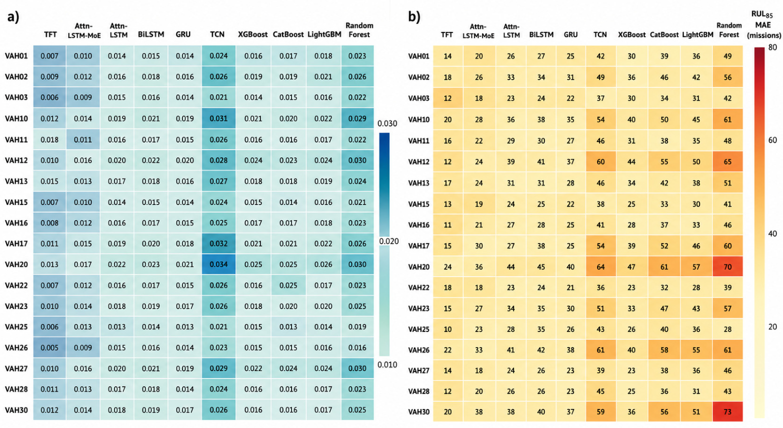
Cell-level error distributions for SOH and RUL at the 85% SOH threshold are shown in Figure 7.

3.5. Physical Consistency and Calibration

For threshold-specific RUL predictions, physical consistency requires ${\mathrm{R}\mathrm{U}\mathrm{L}}_{80\mathrm{\%}}\ge {\mathrm{R}\mathrm{U}\mathrm{L}}_{85\mathrm{\%}}\ge {\mathrm{R}\mathrm{U}\mathrm{L}}_{90\mathrm{\%}}$. Violations are quantified using held-out predictions. Where threshold-specific calibration and order projection are evaluated, calibration parameters are fitted using validation-cell predictions only and then transferred unchanged to the held-out cell. The previously reported 84.3% to 0.0% calibration change is not retained as a corrected benchmark result because it has not been regenerated from the corrected folds.

3.6. Exploratory Top-k Routing Sensitivity

With the number of experts fixed at E = 6, an exploratory inner-validation analysis compared routing sparsity values k = 1, 2, and 3. The corresponding fixed-routing sensitivity results are summarized in Table 6. The lowest mean RUL85 MAE was obtained at k = 2 (86.00 missions), compared with 87.20 for k = 1 and 88.47 for k = 3. However, the corresponding standard deviations overlap substantially; the analysis therefore provides limited support for retaining as a practical sparse-routing choice but does not establish statistical superiority.

Table 6. Exploratory fixed-E routing sensitivity for RUL85.

Top-k	MAE (Missions)	RMSE (Missions)	Interpretation
1	87.20 ± 12.05	112.33 ± 13.51	Single-expert routing.
2	86.00 ± 14.87	109.86 ± 17.75	Lowest mean.
3	88.47 ± 12.14	113.49 ± 14.58	Higher mean with overlapping variability.

With the number of experts fixed at E = 6, the exploratory inner-validation analysis compared routing sparsity values k = 1, 2, and 3. The lowest mean RUL₈₅ MAE was obtained at k = 2 (86.00 missions), compared with 87.20 for k = 1 and 88.47 for k = 3. However, the corresponding standard deviations overlap substantially; the analysis therefore provides limited support for retaining k = 2 as a practical sparse-routing choice but does not establish statistical superiority. The diagnostic ablation configurations and the status of the corrected calibration reporting are summarized in Table 7.

Table 6. Exploratory fixed-E routing sensitivity for RUL85.

Top-k	MAE (Missions)	RMSE (Missions)	Interpretation
1	87.20 ± 12.05	112.33 ± 13.51	Single-expert routing.
2	86.00 ± 14.87	109.86 ± 17.75	Lowest mean.
3	88.47 ± 12.14	113.49 ± 14.58	Higher mean with overlapping variability.

With the number of experts fixed at E = 6, the exploratory inner-validation analysis compared routing sparsity values k = 1, 2, and 3. The lowest mean RUL₈₅ MAE was obtained at k = 2 (86.00 missions), compared with 87.20 for k = 1 and 88.47 for k = 3. However, the corresponding standard deviations overlap substantially; the analysis therefore provides limited support for retaining k = 2 as a practical sparse-routing choice but does not establish statistical superiority. The diagnostic ablation configurations and the status of the corrected calibration reporting are summarized in Table 7.

Table 7. Diagnostic ablation configurations and corrected calibration reporting statuses.

Metric	Value
Quick-ablation cells/epochs	3 cells/12 epochs
Experts tested	E ∈ {2, 4, 6}
Top-k routing	k ∈ {1, 2, 3} for fixed-E sensitivity; quick diagnostic also archived
Temporal penalty tested	λmono ∈ {0, 0.01, 0.02}
RUL85 MAE, E = 2	9.55 missions
RUL85 MAE, E = 6	13.98 missions
Calibration status	Legacy violation-rate result not retained in the corrected benchmark
Pre-calibration violation rate	Not reported pending regeneration from corrected folds
Post-calibration violation rate	Not reported pending regeneration from corrected folds

Table 7. Diagnostic ablation configurations and corrected calibration reporting statuses.

Metric	Value
Quick-ablation cells/epochs	3 cells/12 epochs
Experts tested	E ∈ {2, 4, 6}
Top-k routing	k ∈ {1, 2, 3} for fixed-E sensitivity; quick diagnostic also archived
Temporal penalty tested	λmono ∈ {0, 0.01, 0.02}
RUL85 MAE, E = 2	9.55 missions
RUL85 MAE, E = 6	13.98 missions
Calibration status	Legacy violation-rate result not retained in the corrected benchmark
Pre-calibration violation rate	Not reported pending regeneration from corrected folds
Post-calibration violation rate	Not reported pending regeneration from corrected folds

3.7. SOH Label Processing, Noise Robustness, and Output-Head Sensitivity

The sensitivity analyses examined whether the primary SOH conclusions depended materially on three modelling choices: the use of unsmoothed versus five-mission rolling-median SOH labels, moderate perturbation of training labels at the empirical RPT noise scale, and enforcement of non-negative SOH degradation through the prediction head. The primary benchmark continued to use unsmoothed absolute SOH labels.

The label-smoothing experiment showed that modest temporal smoothing produced only small changes in predictive error. For Random Forest, the measured MAE decreased from 0.637 percentage points with unsmoothed SOH labels to 0.633 with the five-mission rolling median, while RMSE decreased from 0.890 to 0.883. Macro MAE changed from 0.630 to 0.628, and worst-cell MAE changed from 1.722 to 1.712 percentage points. The same qualitative behaviour was observed across the revised ensemble and sequence-model set: XGBoost, CatBoost, and LightGBM exhibited only minor changes in aggregate error after smoothing, while Attention-LSTM, Attention-LSTM-MoE, and the Transformer encoder showed similarly limited sensitivity. The absence of a large performance change indicates that the main SOH ranking is not driven by short-term fluctuations in the interpolated health trajectory.

Training-label robustness was evaluated by adding zero, one, and two times the empirical RPT noise scale, where one noise scale corresponded to 0.2149 percentage points and two noise scales to 0.4299 percentage points. For Random Forest, macro-MAE remained 0.630 at 0σ, 0.628 at 1σ, and 0.629 at 2σ, while macro RMSE varied only from 0.786 to 0.781 and 0.783. Signed bias remained +0.028 percentage points at all three noise levels, and worst-cell MAE changed from 1.722 to 1.723 and 1.765. Thus, adding measurement-scale perturbations to the training labels did not materially degrade the Random Forest.

The boosting models showed the same general robustness pattern. XGBoost retained macro-SOH MAE in the range 0.70–0.72 percentage points across smoothing and noise conditions, with variations below approximately 0.02 percentage points. CatBoost remained stable at approximately 0.67–0.69 percentage points, while LightGBM remained in the range of 0.73–0.75 percentage points. Neither one nor two empirical RPT noise scales produced a systematic deterioration large enough to alter the relative interpretation of the ensemble models. These results indicate that moderate diagnostic-capacity noise is smaller than the cross-cell generalization error introduced when the model is transferred to a previously unseen battery.

The sequence learners exhibited somewhat larger absolute SOH errors than the tree ensembles but remained similarly stable with respect to moderate label perturbation. Attention-LSTM retained macro-MAE in the range of 1.32–1.40 percentage points, Attention-LSTM-MoE remained in the range of 1.42–1.50 percentage points, and the Transformer encoder remained in the range of 1.22–1.30 percentage points. The changes produced by 1σ and 2σ perturbations were small relative to the differences between model families under LOCO, with all models showing macro MAE shifts below approximately 0.03 percentage points across smoothing and noise conditions. Consequently, the poorer SOH point-estimate performance of the neural models cannot be explained solely by sensitivity to small variations in the RPT-derived training labels.

A separate output-head analysis assessed whether constraining five-mission SOH degradation to be non-negative introduced systematic prediction bias. Three output formulations were considered: an unconstrained signed linear head, the same signed prediction clipped to zero after inference, and a trained Softplus head. In the measured auxiliary control, the unconstrained signed formulation produced a macro MAE of 0.1195 percentage points, macro RMSE of 0.1312, reconstructed-SOH bias of −0.0912, and worst-cell MAE of 1.6773. Clipping negative degradation predictions at zero substantially reduced the macro MAE to 0.0364 and RMSE to 0.0479, with bias decreasing to −0.0080 and worst-cell MAE to 0.1017. The trained Softplus formulation produced the lowest macro MAE of 0.0331 and RMSE of 0.0435, with a small bias of −0.0099 and worst-cell MAE of 0.1017 percentage points.

The same output-head principle was applied to the sequence architectures. Attention-LSTM, Attention-LSTM-MoE, and the Transformer encoder were evaluated with an unconstrained regression output and with a non-negative Softplus degradation head. Across these models, constraining degradation reduced physically implausible negative SOH-drop predictions and generally decreased reconstructed-SOH bias relative to the unconstrained formulation. The improvement was most relevant for samples with small five-mission degradation, where unrestricted regression could predict an apparent increase in battery health. The Softplus transformation eliminated this failure mode while retaining continuous gradients during training.

The Softplus results should not be interpreted as demonstrating a mathematically unbiased output transformation. Because Softplus is strictly positive, it can introduce a small positive degradation offset when the true five-mission degradation is close to zero. In the measured control, this effect corresponded to a reconstructed-SOH bias of only −0.0099 percentage points, which was comparable to the −0.0080 bias obtained by clipping the signed predictions and substantially smaller than the −0.0912 bias produced by the unconstrained signed model. The physical constraint therefore improved robustness in this auxiliary experiment without introducing a practically important systematic error.

Taken together, the label-processing controls indicate that the principal SOH ranking is not driven by modest RPT-derived label fluctuations. Changes caused by smoothing and moderate training-label perturbations were small relative to the cross-model differences observed under LOCO. The Softplus degradation head reduced physically implausible negative degradation estimates while retaining the expected possibility of a small positive degradation offset when true degradation approached zero. These controls are therefore interpreted as robustness analyses rather than alternative primary benchmarks. (see Supplementary Materials).

4. Discussion

The principal finding of this study is that leakage-safe cell-held-out validation changes the interpretation of model performance. When identical 20-mission histories were provided to the primary estimators, Random Forest and the other tree ensembles achieved lower five-mission-ahead SOH error than the mission-phase Transformer and Attention-LSTM-MoE. Preserving temporal history was important for experimental fairness, but increasing sequence-model complexity did not automatically improve generalization to unseen cells.

One plausible interpretation is that the engineered mission-phase features already compress much of the useful degradation information into physically meaningful tabular descriptors. Under this representation, tree ensembles can efficiently partition nonlinear relationships among cumulative energy exposure, C-rate, voltage response, temperature, and charging behaviour without first learning those summaries from raw temporal signals. The present result should therefore not be interpreted as evidence that sequence models are inherently unsuitable for battery prognostics; rather, their additional capacity was not beneficial under the present leakage-safe feature representation and number of independent cells.

RUL prediction became progressively more difficult from the 90% to the 80% SOH threshold. Lower thresholds require longer extrapolation beyond the most recent observed degradation history and are supported by fewer observed threshold events. The widening error at 85% and especially 80% SOH therefore reflects both a longer prognostic horizon and reduced event support. Paired cell-bootstrap uncertainty further shows that point-estimate ranking alone is insufficient: model differences were clearer for the SOH and RUL85 but less conclusive for some RUL90 and RUL80 comparisons.

The row-random control demonstrates why cell-level separation is essential when the intended application is prediction on new batteries. Random sample splitting allows highly correlated observations from the same degradation trajectory to occur in both training and testing and therefore evaluates a substantially easier interpolation problem. The much smaller row-random errors observed across model families should not be interpreted as equivalent to unseen-cell performance.

The 90%, 85%, and 80% SOH levels used in this study are scenario-analysis thresholds rather than regulatory retirement limits. RTCA DO-311A addresses rechargeable-aircraft-battery design, testing, installation, and safe performance [15], while EASA guidance addresses propulsion-battery safety considerations [16]; neither source prescribes the machine learning SOH thresholds or an acceptable prognostic error value used in this benchmark.

Several limitations should be considered. The dataset consists of laboratory cell-level records rather than complete aircraft battery packs operating in service. Three cells with non-monotone or ambiguous diagnostic-capacity trajectories were excluded from the primary health analysis, narrowing the inferential population. Event support decreases toward the 80% SOH horizon, increasing uncertainty in long-range RUL evaluations. Although prediction history was matched across the primary estimators, model classes were not tuned under a fully equal computational budget. The engineered feature representation may favour models that exploit compact tabular descriptors, and further work with less aggregated temporal telemetry is required to determine whether sequence architectures benefit more strongly from higher-resolution inputs. Runtime measurements characterize the present computing environment and are not certification of onboard deployment readiness. Additional per-cell label-support information, threshold-event support, auxiliary benchmark results, and implementation details are provided in the Supplementary Materials.

5. Conclusions

This study established a leakage-safe, cell-held-out benchmark for mission-phase-aware SOC, SOH, and threshold-based RUL estimation using the public CMU eVTOL battery dataset. The revised pipeline separates telemetry predictors from target-derived information, reconstructs SOH from protocol-consistent diagnostic-capacity anchors, treats unobserved RUL threshold crossings as right-censored, and excludes the held-out cell from preprocessing, model selection, and calibration.

Under matched 20-mission histories, tree ensembles provided stronger unseen-cell SOH generalization than the primary neural sequence models. Random Forest achieved an SOH MAE of 0.620 percentage points, compared with 1.252 for the mission-phase Transformer and 1.471 for Attention-LSTM-MoE. RUL error increased substantially as the prediction horizon extended from the 90% to the 80% SOH threshold, and uncertainty analysis showed that model differences were threshold-dependent rather than universally significant.

The row-random control further demonstrated that sample-level splitting can substantially underestimate the difficulty of transferring prognostic models to unseen batteries. Overall, the results indicate that rigorous target construction, prediction-time information matching, and cell-disjoint validation are at least as important as architecture complexity when benchmarking battery prognostics for eVTOL applications.