


Abstract
Continuous twin-screw extrusion of graphite anode slurries operates in a narrow window: too little kneading leaves carbon black agglomerates, and too much fractures the graphite. Existing studies collapse both defects into a single pass/fail criterion, which is ambiguous because the two are distinct phenomena that no single measurand resolves. This study resolves the upstream half of the causal chain, from extrusion parameters to the high-shear slurry viscosity ; the downstream half, from through electrode tortuosity to fast-charge performance, was established for the same material system and process line in a companion study, so that the two are complementary rather than overlapping. A graphite peak width criterion () combined with grindometer screening reduces 114 trials to 54 in which, within the detection limits of the two methods, no particle-related cause of viscosity variation remains identifiable, and 52 of these with a recorded specific mechanical energy form the modelling dataset. Two logistic regressions show that the two failure modes are predicted from the machine settings with markedly different sharpness: particle damage by kneading concentration and kneading length (AUC = 0.955, 0.914 under cross-validation) and agglomerate removal by backward elements and screw speed (AUC = 0.740), with backward elements entering both models with opposite signs as the central design trade-off. Inside the window the specific mechanical energy is a genuine but coarse descriptor: after compositional normalisation it accounts for 57% of the viscosity variance, yet it places individual operating points to only 9.5% mean relative error, and pairs of runs receiving the same energy differ by up to 49% in viscosity, so it cannot serve as the descriptor of the network state. A greybox model with eight free parameters reproduces the compositionally normalised viscosity to 5.0% mean relative error, gating a kneading term against a low-concentration path through a sigmoid at , and attains a leave-one-out of 0.796, where a twenty-one-term response surface benchmark fitted by the same protocol collapses out of sample. Its training error is of the order of the pooled replicate scatter of the process itself.
1. Introduction
1.1. The Rheological Bottleneck in Fast-Charge Anodes
Fast charging is the most frequently cited barrier to electric vehicle adoption, and the graphite anode is its bottleneck [1,2]. Lithium ions must reach the active material through the electrode pore network; where tortuosity is excessive, concentration polarisation drives the local anode potential below the plating threshold and capacity fades [3,4]. Tortuosity is set during drying by the spatial distribution of the carbon-binder domain (CBD), which is inherited from the rheological state of the slurry at the moment of coating [5].
The high-shear viscosity at = 100 s−1, hereafter , is therefore more than a quality attribute. It reports the conformational state of the carboxymethyl cellulose (CMC) binder that governs CBD migration and pore blockage during drying [6,7]. Scheutjens–Fleer theory describes adsorbed polymer through trains in direct surface contact, loops protruding into solution and free tails [8,9], and the shift from extended loop–tail configurations towards flat train conformations is the molecular mechanism that couples mixing intensity to electrode microstructure.
This chain has been quantified for the present material system on the present extruder line. In a companion study, kneading conditions that left graphite particle size distribution and crystallinity unchanged nevertheless yielded electrodes differing by 17% in effective tortuosity and by 14.9% in 8–80% SOC charging time, with tortuosity explaining the fast-charge response () far better than interfacial kinetics () [10]. Because graphite particle size distribution and crystallinity were unchanged, the performance difference must be sought in the binder network rather than in the active material, that is, in the state reports. Inside a damage-free process window, is therefore the accessible manifestation of the microstructure-determining variable, and that is what justifies modelling it as a function of extrusion parameters.
1.2. Twin-Screw Extrusion and the Ambiguity of a Single Failure Criterion
Twin-screw extrusion (TSE) is an established continuous mixing technology for producing these slurries at scale, offering narrow residence time distributions and inline monitoring capability [11,12,13,14,15,16]. The open question is how to set the seven available process parameters so as to reach a target without damaging the graphite.
Prior TSE studies on electrode slurries have produced valuable empirical data [17,18,19,20,21] but share a structural weakness, in that particle breakage and agglomerate persistence are usually merged into one binary “not OK” classification [17,18]. This is ambiguous, because a broadened graphite peak and a failed grindometer test report different phenomena on different measurands: the first an excess of fines generated by fracture, the second residual coarse clusters that survive processing. Neither measurand substitutes for the other, since laser diffraction requires a dilution step that disaggregates precisely those clusters. Superimposing them in a single target variable forecloses mechanistic interpretation and can misdirect optimisation. The same corrective action, more kneading, cures one defect and causes the other. Terashita and Miyanami [22] showed early on that stepwise thickener addition improves dispersion quality, and Borzutzki et al. [17] located a reversal point near 80 wt% kneading concentration beyond which carbon black dispersion gains give way to graphite fragmentation. Neither separated the statistical drivers of the two failure modes, which is the prerequisite for interpreting any downstream rheological measurement.
1.3. Why a Scalar Energy Metric Is Not Enough
A second gap concerns the descriptor used to summarise the process. Viscosity modelling for electrode slurries remains confined to response surface methodology and polynomial regression [23,24], whose coefficients carry no mechanistic content, since a significant interaction term indicates correlation and no mechanism. Hybrid and physics-informed architectures address exactly this deficit [25,26,27]. Perera et al. [28] reduced polymer extrusion prediction error by 16% with a physics-informed network, and Zhang et al. [29] achieved 90–97% MSE reduction for cement slurry viscosity. We are not aware of an equivalent model for electrode slurries.
A third gap is more fundamental. The specific mechanical energy (SME) integrates torque over residence time into a single number, so it carries the macroscopic process effort but no published model separates the intensity of stress transmission from the duration of exposure. The same energy input can arise from brief intense loading, prolonged moderate exposure, elevated back-pressure, an altered degree of fill, or stronger wall slip. In a highly filled suspension, these are not equivalent states. What matters is not only how much energy enters, but also where, for how long, and at which local solid concentration it is transmitted. A descriptor that averages over this distinction cannot resolve it.
1.4. Objectives, Hypothesis and Contribution
The hypothesis of this work is that particle damage and agglomerate persistence are not two manifestations of one “mixing intensity” variable but distinct failure modes that the machine settings predict with different sharpness, and that within the resulting damage-free window the residual viscosity variation is governed by a concentration-gated, exposure-controlled restructuring of the CMC network that can be decomposed into separable intensity and time contributions.
Three contributions follow. First, we establish the decoupling of the two failure modes as a methodological precondition for rheological modelling, not as a standalone result, and we quantify it: the two failure modes are governed by different parameter hierarchies and are predicted from the machine settings with markedly different sharpness, yet are coupled through one shared design variable. Second, we quantify what a scalar energy metric can and cannot do within the damage-free window: on a compositionally normalised basis it carries more than half of the viscosity variance, so it is not uninformative, but it resolves individual operating points to only about 10% and runs receiving the same energy reach substantially different network states, so it is not a usable optimisation target. Third, we formulate a greybox viscosity model in which every parameter maps to an identifiable process quantity, whose activation threshold coincides with the particle damage boundary, and whose exposure variable is the classical dimensionless throughput number, so that the model is expressed in scale-transferable quantities from the outset.
Two claims are deliberately not made. The model is written in scale-transferable quantities, but scale transfer itself is not demonstrated, since all experiments were performed on one barrel diameter. And no molecular mechanism is identified: the fitted threshold is a regime boundary of an operational process variable, and the adsorbed-layer reading of Section 3.2.2 is an interpretation compatible with the data rather than a measurement.
Delimitation from the Companion Study
This work and the companion publication [10] share a material system, an extruder line and a design of experiments, and they address opposite halves of the same causal chain; neither reproduces the other. The companion study takes the coated electrode as its object and resolves the downstream link: how the slurry network state governs carbon-binder-domain redistribution during drying, hence pore morphology and effective tortuosity, and hence the 8–80% SOC charging time of full cells. Its terminal response is electrochemical. The present study takes the extruder as its object and resolves the upstream link: how the seven process parameters, through a concentration-gated stress intensity and its cumulative exposure, determine the high-shear viscosity that reports that network state. Its terminal response is rheological, and no cell is built here. The junction between the two is , which is the dependent variable in this study and the independent variable in the companion one.
The separation is complete in both directions. Neither the two-criterion process window, the logistic classification of the failure modes, the compositional capability analysis, the response surface benchmark nor the greybox model appears in [10]. Conversely, no coating trial, pore-structure measurement, tortuosity determination, impedance spectrum, distribution-of-relaxation-times analysis or cell-level charging result appears here. Findings from the companion study are cited in this manuscript for one purpose only, namely to justify why is a response worth modelling at all, and they are marked as such wherever they occur.
2. Experimental Methods
2.1. Materials
The anode formulation comprised a synthetic graphite carrying an amorphous carbon coating ( µm, BET 4.85 m2 g−1), Super C45 carbon black (Imerys Graphite & Carbon, Bodio, Switzerland; BET 45 m2 g−1), sodium carboxymethyl cellulose (CMC, MAC500L, Nippon Paper Industries Co., Ltd., Tokyo, Japan; = 344,440 g mol−1, DS = 0.70), and an aqueous styrene–butadiene rubber latex dispersion (SBR, Zeon 451-B, Zeon Corporation, Tokyo, Japan; 40 wt%) in a dry mass ratio of 96:1:1:2. This composition is an industrially representative high-energy anode formulation and was held constant throughout, so that the seven process variables could be varied without confounding by formulation. It is the same composition as in the companion study [10], which is what allows the rheological and the electrode-level results to be joined. The graphite is comparatively fine and correspondingly prone to agglomeration, which makes it a demanding material system to process [17,18]. An aqueous CMC master solution (1.4 wt% in deionised water, the highest concentration that remained reliably pumpable for the downstream eccentric screw pumps) was prepared in 180 L batches on an inline powder-wetting and dispersing unit working on the rotor–stator principle; four such batches covered the entire experimental campaign. The CMC was drawn in and distributed for 10 min at 1500 rpm and then swollen for 10 min at 1000 rpm, throughout at 20 °C. The solution was then transferred to supply containers and held under slow agitation until the following day, so that the CMC swells completely and the solution degasses [6,30]. Each batch was verified gravimetrically against the nominal 1.4 wt% on two 25 g samples with an accepted deviation of ±2%, and was additionally checked rheologically.
2.2. Twin-Screw Extrusion Process
Continuous mixing was performed on a co-rotating intermeshing twin-screw extruder (BTSK 30/44, Bühler AG, Uzwil, Switzerland; screw diameter = 30 mm, screw length 1720 mm, , modular build of 14 barrel sections) operated at pilot scale. All results reported here were obtained on that pilot line and not on a production line. This aspect ratio falls between pharmaceutical hot-melt extruders (–40) [31,32] and polymer compounding systems (–52) [33,34]. The screw configuration comprised functional zones for solid feeding, CMC solution injection and wetting, high-solid kneading ( = 60–80 wt%), and SBR latex addition with final dilution to the target solid content ( = 56.0 wt%). The extruder ran starve-fed, so throughput is set by external gravimetric feeders independently of screw speed [33,35].
The kneading-zone solid concentration is an operational set point of this line. Liquid can be injected between barrel sections 2 and 14; two independently controlled lines feed the CMC master solution from a common supply vessel, and the split between them is what sets . The first fraction is injected upstream of the kneading section, so that together with the gravimetrically fed solids, it fixes the solid concentration through the two kneading zones in barrel sections 3–4 and 6–7. The remaining CMC solution, the balance of the dilution water and the SBR dispersion are added distributively from barrel section 8 onwards and set the final solid content. All liquid streams are metered by eccentric screw pumps and monitored by Coriolis flow metres. The corresponding feed-stream mass balance is given in Supplementary Note S12 and its consequences for the interpretation of the fitted concentration threshold are discussed in Section 3.2.5.
2.3. Design of Experiments
Seven process parameters were varied systematically (Figure 1): throughput (, 25–55 kg h−1), screw speed (n, 600–1200 rpm), kneading concentration (, 60–80 wt%), kneading length (, 7–50%, a relative length denoted where it enters the viscosity models), and the counts of forward polygon elements (, 0–20), backward polygon elements (, 0–10) and turbo mixing elements (, 0–6).
Figure 1.
Overview of the seven process parameters and the design of experiments. (Top): Barrel and feed-stream schematic of the extruder over its fourteen barrel sections, with the powder and liquid feed points, the solid content along the process length, and the split of the CMC master solution that sets in the kneading zone. (Bottom): The three designs of experiments, executed one after another to build up the model description, progressing from fractional factorial screening (34 runs, resolution IV) through Box–Behnken optimisation (60 runs) to the higher resolution stage (20 runs, including the 11-point sweep). Together the three stages comprise the 114 experiments, which span the full accessible parameter space of the Bühler BTSK 30/44 extruder.
The seven variables were covered by a single design of experiments assembled in three sequential stages (Figure 1): a fractional factorial screening stage (34 runs, resolution IV, in duplicate), a Box–Behnken optimisation stage (60 runs with screw elements disaggregated) [23], and a higher resolution stage (20 runs including an 11-point sweep for threshold determination), yielding 114 experiments in total. The escalation within the design follows the standard progression of resolution: the screening stage identifies which of the seven variables carry the two failure modes, the Box–Behnken stage resolves curvature and two-factor interactions among the retained variables, and the third stage places additional points where the first two indicated a transition. Screw configurations were drawn from a systematic family of 21 parameterised builds (SD1–SD21) at a fixed element sequence and symmetric arrangement about a central conveying element, so that element counts enter the models as controlled numerical factors instead of categorical design identifiers; Supplementary Note S1 and Figure S1 document the three stages of the design and the complete screw-design family.
A sequential design concentrates observations where earlier stages indicated structure, so the resulting dataset is not balanced across the factor levels. Section 3.1.6 quantifies the consequences of this, together with those of the subsequent curation.
2.4. Slurry Characterisation
2.4.1. Shear Viscosity
Flow curves were acquired on a rotational rheometer (Kinexus Pro+, Netzsch-Gerätebau GmbH, Selb, Germany; cone-plate geometry CP 1°/50 mm, 20.0 ± 0.1 °C) over a logarithmic shear rate ramp of 0.1–1000 s−1, each preceded by a conditioning step at 0.1 s−1 for 30 s to suppress loading artefacts at the first point of the ramp [36,37]. Evaporation was limited by a solvent trap and by a total measurement time of about 12 min. The viscosity at = 100 s−1 is reported in Pa s throughout and spans 1.49–3.16 Pa s across the curated dataset, and 1.50–2.99 Pa s after the compositional normalisation of Section 3.2.1. It served as the primary response for two reasons. This shear rate is representative of the hydrodynamic regime in the feed and manifold of a slot-die coater [38,39], though not of the die lip, where rates are one to three orders of magnitude higher. And inside the damage-free window, it responds to binder distribution and network topology, which govern the pore morphology and tortuosity of the dried electrode produced on this line [10].
One convention applies to every figure of this work. The viscosity axes are labelled without a subscript distinguishing the uncorrected response from the compositionally normalised of Section 3.2.1, so that axes remain directly comparable across figures and models; which of the two is plotted is stated in the caption of each figure. The tables carry the subscripts throughout, and the numerical difference between the two responses is quantified in Section 3.2.6.
The choice of a single shear rate is a restriction of the present work. Yield stress and zero-shear viscosity report the low-shear, structure-dominated regime that governs sedimentation stability and coating start-up, and they are not represented here; extending the response to a low-shear descriptor is the most direct enlargement of the framework.
The measurement temperature of 20.0 ± 0.1 °C is a comparison condition and not the process temperature. The barrel is temperature-controlled in six circuits held to ±1 °C on their set points during sampling, but the slurry temperature at the die exit was not controlled to the tolerance of the rheometer, and the temperature dependence of was not measured; Section 3.4 states the consequence.
2.4.2. Particle Size Analysis
Particle size distributions were measured by laser diffraction (Mastersizer 3000, Malvern Panalytical Ltd., Malvern, Worcestershire, UK) with a wet dispersion unit (deionised water). For each measurement 0.5 g of slurry was diluted with 1.5 g of deionised water and stirred for two to three minutes until no lumps remained; one to two drops were then transferred into the wet dispersion unit and the obscuration was set within the range recommended by the manufacturer. At least three measurement points were recorded per sample. The graphite peak width , defined in Section 3.1.1, served as the primary particle integrity criterion because it responds to incipient attrition earlier than the median . Repeat measurements on identical samples give for (coefficient of variation ≈ 1.8%) and ±0.3 µm for .
Dilution disaggregates weakly bonded clusters, so the measurement reports graphite fracture and not agglomeration; fracture itself is irreversible and is not created or removed by the sample preparation. This is also why an independent criterion on the undiluted slurry is required, and Section 2.4.3 describes it.
2.4.3. Grindometer Testing
A grindometer test (Hegman gauge, DIN EN ISO 1524 [40]; wedge-shaped groove, measuring range 0–50 µm, drawn down on a plane-parallel steel bed) was applied to all samples as a complementary agglomerate screen. Only particle assemblies whose dimension exceeds the local groove depth are registered, so the practical detection limit of the instrument used is about 15 µm; submicron carbon black networks and internal graphite defects remain undetected. Together with the repeatability of this fixes what the phrase within the detection limits of the two criteria means wherever it is used below. This second criterion is indispensable rather than confirmatory. Laser diffraction requires dilution in water, which disaggregates weakly bonded clusters that are stable under process-relevant shear yet raise the high-shear viscosity through an increased effective volume fraction. Left undetected, they would masquerade as CMC network effects, which is precisely the misattribution this study is designed to avoid. Samples that satisfied the width criterion but failed the grindometer test (scratch depth > 40 µm) were excluded from the curated dataset.
2.5. Experimental Protocol and Sources of Variability
Solid content was determined gravimetrically on a precision balance with an integrated heating element: 2–2.5 g of slurry was dried at 130 °C until the mass stayed constant over several minutes, with one determination per run and 114 determinations in total. Specific mechanical energy was computed from the measured shaft torque after subtraction of the no-load torque, integrated over the sampling window and divided by the mass throughput. Before every run the extruder was conditioned for 30 min at 600 rpm with a water flow of 5 L/h−1, so that barrel temperature control, drive and screws reached a stationary state and the torque signal was free of start-up transients; the no-load reference was taken at this condition, that is, once per run and not once per campaign. Samples were withdrawn at the die exit once all six temperature-control circuits held their set points to within ±1 °C and the torque signal was stationary. At least 1 L of slurry was taken per run and homogenised by swirling for 30 s before analysis. This pre-treatment is not structure-neutral, since the three-interval thixotropy test on this material system shows network recovery on a scale of minutes, but it is identical for every sample, so that comparisons between operating points remain valid while absolute low-shear values are to be read as pre-sheared.
The specific mechanical energy is a derived quantity and not a model input: it enters neither the response surface model nor the greybox model, and it is used only for the correlation of Section 3.2.3. Its run-to-run reproducibility is correspondingly modest. Over the seven groups of repeated settings, the pure-error standard deviation of is 0.366 on eight degrees of freedom, so that the pure-error variance is about 35% of its total variance, and a log-linear regression of on the seven process variables explains only 24% of it. Torque on a starve-fed machine responds to fill state and wall condition as well as to the set points, so the energy signal carries run-specific information that the settings do not reproduce. Section 3.2.3 draws its conclusion accordingly, and the column used for that fit is the one published in Supplementary Table S2.
The three stages were executed as consecutive campaign blocks, in the order screening, Box–Behnken and resolution stage, spread over several production months. Randomisation of the run order against the campaign sequence was not part of the protocol, so the block index cannot be separated from a possible time trend; this is a restriction of the design and is stated as such rather than corrected after the fact.
Over those months the campaign drew on four 180 L batches of CMC master solution, so a change in batch is a further possible block effect. It was not entered as a block factor. Two observations bound it. Every batch was controlled gravimetrically to 1.4 wt% within ±2% and additionally checked rheologically, so that concentration and dissolution state stayed within narrow limits. And the centre points, distributed over the entire period, returned repeatedly similar viscosities, where a dominant batch effect would have been visible. The residual contribution is contained in the pooled replicate scatter quantified below.
The modelling dataset contains seven groups of repeated settings comprising 15 runs, with eight degrees of freedom in total. The pooled pure-error standard deviation over all seven groups is 0.1898 Pa s on the compositionally normalised response, a coefficient of variation of 7.9% against the dataset mean of 2.40 Pa s. On the uncorrected response the same calculation gives 0.2993 Pa s, or 12.5%, and the difference between the two is the clearest single measure of what the compositional normalisation of Section 3.2.1 achieves. The replicates are not distributed uniformly over the design space, being concentrated at the centre point and within the screening design, with no replication inside the concentration ramp. The pooled estimate should therefore be read as a representative rather than a spatially resolved measure of reproducibility.
The four CMC master solution batches were each prepared in 180 L on the day before first use and held at 20 °C under slow agitation in the supply vessel; a batch of that size served several consecutive production days, so the ageing time of the solution actually dosed ranges from one night to several days and was not controlled to a fixed upper limit. The batch records are available from the corresponding author on request. Slurry sampled at the die exit was transferred directly into the sample vessel, held there at room temperature, and characterised rheologically within 15 min of sampling in every case. Neither the ageing time of the master solution nor the process temperature was varied systematically, so their contribution to the residual scatter is bounded by the protocol but not quantified.
No observation was removed from the modelling dataset as an outlier. All six models of Section 3.2 are fitted on the same 52 runs, in the same row order, so that every figure of merit in Section 3.2.6 refers to an identical sample.
2.6. Statistical Methods
2.6.1. Binary Logistic Regression
Two separate binary logistic regressions were fitted on the full 114-experiment dataset (Minitab 21, Minitab LLC, State College, PA, USA) using forward stepwise selection based on the likelihood ratio test with a deliberately liberal entry criterion (), because the aim is comprehensive identification of contributing parameters, not a parsimonious inferential model. Logistic regression was chosen over more flexible classifiers for two reasons: the purpose is to identify which process parameters carry which failure mode and with what sign, and the predicted probabilities are required to be calibrated so that they can serve directly as operating limits in Section 3.1.5. With 114 observations and 16 damage events, a random forest or a neural network would in addition not support the parameter hierarchy on which the decoupling argument rests.
Quality is reported in the main text as the area under the receiver operating characteristic curve (AUC) and the corrected deviance . The calibration and rank-correlation diagnostics used to support them, namely the Hosmer–Lemeshow goodness-of-fit test across ten risk bands and Somers’ D, together with the scale on which pseudo- measures must be read, are set out in Supplementary Note S3 [41]. No variance inflation factor among the retained predictors exceeds 3.5, so linear dependence among them does not distort the reported effect sizes.
2.6.2. Response Surface Model
The modelling was implemented in Python 3.9.12 using the Anaconda platform (Conda 4.12.0) and executed in a JupyterLab 3.3.2 environment. Data processing and statistical analysis were developed using standard Python scientific computing libraries. Three decisions frame it. A Box–Cox analysis over the family of power transformations returned as the optimal variance-stabilising transformation, which by convention is the natural logarithm [42]. The model response is therefore
Equation (1) stabilises the mean-proportional heteroscedasticity typical of suspension rheology, converts multiplicative process influences into additive contributions, and makes the back-transformed prediction strictly positive by construction. The back-transformation returns the conditional median rather than the mean; the Duan smearing factor is 1.0022, so the difference is systematic but small. Supplementary Note S5 develops the three arguments [43].
All seven process variables were mean-centred and scaled to unit standard deviation (Supplementary Table S5),
which renders the coded coefficients comparable as dimensionless effect sizes and suppresses the artificial correlation between linear and quadratic terms, since after centring z and are approximately orthogonal.
Terms were removed from the full model, comprising the seven linear main effects, their quadratic terms and all 21 two-way interactions, by backward elimination at , with non-significant parent terms of retained higher-order effects kept to preserve the hierarchy principle [44]. Because the term structure is selected from the data, the standard errors and p values of the final model are conditional on that selection and are to be read as a ranking of effects rather than as significance proofs.
Multicollinearity among the retained terms was monitored through the maximum variance inflation factor (8.13), the maximum absolute parameter correlation (0.888) and the condition number of the standardised design matrix () [45]. None of these is pathological, but all three are markedly larger than for a reduced model, which is the first quantitative sign of what the term count costs.
One decision about the cross-validation deserves emphasis, because it governs the comparison of Section 3.2.6. Backward elimination is part of the model building, not a preprocessing step, so it is repeated inside every leave-one-out fold on the training rows alone. Holding the term structure of the final model fixed across the folds, which is the more common practice, would let the held-out observation influence its own predictor through the selection and would quantify coefficient uncertainty while suppressing selection uncertainty. On a design of this size the difference is not cosmetic, and Section 3.2.6 reports what the honest protocol returns. Supplementary Note S5 justifies the choice of backward over forward selection and of the liberal removal threshold [24,45].
2.6.3. Greybox Model Fitting
The greybox model was fitted by bound-constrained nonlinear least squares from 49 starts, a default start vector and 48 points drawn uniformly within the search bounds of Supplementary Table S8b, the reported solution being the best of these. On the compositionally normalised response 49 starts converge and 48 of them reach the same optimum, at a residual sum of squares of 1.2734; on the uncorrected response 49 converge and 39 reach the optimum. No parameter comes to rest on a search bound. At the solution the largest absolute correlation between any two parameters is 0.632, between the kneading efficiency and the element weight , which is structural: both scale the same product in Equation (11). Nothing in the set approaches the range in which parameters cease to be separately estimable.
The kneading term of Equation (11) deliberately carries no data-dependent normalisation constant. A factor of the form is absorbed completely into and therefore changes no prediction of the full fit, but under cross-validation the mean would be formed over rows that include the held-out observation, and the element information would enter the held-out prediction through the constant. Writing into the model unscaled removes that path entirely, at no cost in fit. In every leave-one-out fold the model is refitted on the 51 training rows alone, from ten starts: the default start vector, the full-data solution and eight new random points within the bounds, the best of which is kept. The two informed starts only select the basin in which the optimiser converges, since the fold objective contains no information from the held-out run; repeating all 52 folds from 48 random starts without them returns the same held-out predictions to within Pa s and the same on both responses (Supplementary Note S10.4).
Standard errors and confidence intervals from the Wald approximation are local diagnostics of the nonlinear fit and are not significance proofs for the underlying mechanisms. Model discrimination between competing architectural variants used AIC, AICc and BIC together with leave-one-out cross-validation and the maximum absolute parameter correlation as an identifiability indicator.
3. Results and Discussion
3.1. A Two-Criterion Process Window
Process-induced changes in slurry viscosity must not be read as binder or network phenomena, while particle fracture or residual agglomerates remain possible, because the same mechanical loading produces both. This section delimits the domain in which the two confounders are metrologically controlled, and then asks whether they are governed by the same process parameters. Two quantities are measured directly, the graphite peak width from laser diffraction and the maximum scratch depth in the grindometer, and binary criteria are derived from them. The logistic models built on those criteria are offered not as molecular proof but as a measurable representation of two failure modes within the investigated process space. The decision criterion for everything that follows is explicit: the window qualifies for network and viscosity modelling only if the two failure modes are described by different parameter hierarchies instead of one common global over- or under-loading. Only then may later viscosity differences be attributed to the CMC/carbon black binder network with methodological confidence.
3.1.1. Graphite Peak Width as a Damage Indicator
The graphite distribution width is the half-maximum width of the graphite sub-peak of the volume density distribution , evaluated on a logarithmic size axis and normalised by the peak height:
where and are the left and right half-maximum positions and the peak height of on the same axis. Numerator and denominator are both dimensionless, so is dimensionless. Figure 2a shows the distributions from which the quantity is read: the two half-maximum positions are taken on the graphite sub-peak alone, on the logarithmic abscissa of that panel, and divided by the height of the same sub-peak.
Figure 2.
The two-criterion process window across all 114 experiments. (a): Representative particle size distributions coloured by the width criterion. The graphite peak sits at ∼10 µm and carbon black at ∼1.5 µm. Excessive stress generates fragments at ∼2.5 µm and below, which broadens the graphite peak towards small sizes; the pictogram labelled high stress illustrates that fracture case. The width is used here only as an indicator of graphite fracture; residual agglomerates are not resolved by this measurement, because the dilution required for laser diffraction disaggregates them, and they are captured by the grindometer criterion instead. (b): Cumulative distribution of , with the gap at 0.88 magnified in the inset; below the threshold the values rise steeply and continuously, above it they scatter sparsely up to 1.6. (c): Trial counts resolved by parameter level and coloured by the four possible outcomes: process window, active anode material (AAM) damage only, agglomerates only, and both. All four categories are populated, and their ratio stays approximately constant across most levels of most parameters, so no single setting guarantees a clean outcome and none precludes one. (d): Standardised effects of the particle integrity model. and the interaction exceed , as does , whereas the main effect does not. (e): Standardised effects of the agglomerate removal model, dominated by , n and their interaction. The two panels share no dominant term, which is the quantitative form of the decoupling argument; appears in both, with opposite signs. Consistently with Equation (3), is plotted as a dimensionless quantity and carries no unit.
Throughout this work is used only as an indicator of graphite fracture. It cannot report residual agglomerates, because the sample must be diluted in water for the measurement and that step disaggregates the weakly bonded clusters, which is why the grindometer is carried alongside it as an independent criterion (Section 3.1.2). The idea of monitoring distribution width as a damage proxy goes back to the Relative Span Factor introduced by Griessl et al. for monomodal distributions [3]. Since that factor is not applicable to the multimodal distributions present here (graphite peak ∼10 µm, carbon black aggregates ∼1.5 µm), the underlying logic was adapted: Equation (3) evaluates the graphite sub-peak alone and is therefore robust against variations in carbon black content. It is not the span , which for the same distribution takes a different value; Supplementary Note S6 states the distinction explicitly and computes throughout by Equation (3).
Three observations support the threshold, and all three precede any viscosity model. Figure 2b shows the cumulative distribution of over all 114 experiments. A gap appears at , where a steep, continuous rise in tightly clustered data below this value gives way to a sparsely populated zone of widely scattered values extending to 1.6. A bootstrap over 1000 resamples places the gap at (95% CI, median 0.88). Systematic variation in the threshold between 0.85 and 0.90 changes the number of in-window experiments from 54 to between 49 and 57 and moves the fitted greybox parameters well inside their confidence intervals. The grindometer threshold of 40 µm is fixed by the scale gradation of the instrument and was not available as a tuning parameter even in principle. Supplementary Table S4 reports all three checks in full.
The broadening that the criterion detects is directed towards small sizes, with fragment populations appearing at ∼2.5 µm and below the graphite mode (Figure 2a), whereas agglomeration would broaden the distribution towards large sizes. Together with the measurement reproducibility of , which is small against the gap of about 0.1 between the two populations, this is the basis for reading the criterion as an indicator of fracture. It does not quantify the absolute extent of fracture, and it is used here only as a comparative integrity check across processing conditions.
3.1.2. The Combined Window
Combining both criteria retains 54 of 114 experiments. For two of those 54, sequences 28 and 37, no specific mechanical energy was recorded. Because the energy correlation of Section 3.2.3 requires it and all models are compared on an identical sample, both are carried no further, so the modelling dataset of Section 3.2 comprises 52 runs; Supplementary Table S2 reproduces it in full. (All six models of Section 3.2 are fitted on those same 52 rows, in the same order. No model uses a subset of its own, and no observation is excluded as an outlier, so every figure of merit in Section 3.2.6 refers to an identical sample.) Within this domain, and within the detection limits of the two criteria, viscosity variation can no longer be attributed to fracture or to macroscopic agglomerates. The remaining candidates are CMC network and adsorption phenomena, namely polymer conformation, binder redistribution and carbon black network connectivity.
The two criteria address different defects and have different detection limits, and this bounds the claim. The width criterion reports graphite fracture and nothing else, since the dilution required for laser diffraction disaggregates the clusters that the grindometer is there to detect. The grindometer in turn resolves macroscopic agglomerates (>15 µm) but not micro-agglomerates, whose residual contribution to the viscosity scatter cannot be excluded from the present evidence. The curation nevertheless remains the central precondition for everything that follows, because it secures the causal assignment between process parameters and rheological response that the literature convention of a single pass/fail criterion forfeits.
3.1.3. Four-Quadrant Classification
If particle damage and agglomerate persistence traced back to a common cause, both would occur or be absent together, and a cross-classification of the two criteria would populate only its diagonal. Figure 2c resolves all 114 experiments by parameter level and colours them by the four possible outcomes. Of the 114 trials, 54 fall inside the window, 6 show damage while being fully dispersed (high loading intensity with good stress transfer), 44 retain agglomerates with no detectable damage (insufficient hydrodynamic forces at low contact stress), and the remaining 10 exhibit both. The two off-diagonal populations together comprise 50 trials, too large a share to dismiss as scatter and enough to undermine a monocausal description through one global loading intensity.
A second feature of the same panel is easily missed. Within most parameters the ratio of the four outcomes stays approximately constant across levels, so raising or lowering any single setting shifts the balance but never eliminates a failure mode. Kneading concentration is the clearest case; its process window share collapses only at 80 wt%. No univariate limit will therefore define the window, and this is what motivates the multivariate treatment below.
3.1.4. Predictability, Not Model Quality, Separates the Two Regressions
The target variables were particle integrity, with 98 successes against 16 failures at , and agglomerate removal, with 60 successes against 54 failures on the grindometer criterion. Table 1 summarises model quality, and Figure 2d,e shows the standardised effects of both models, whose numerical values are listed in Supplementary Table S3.
Table 1.
Model quality of the two binary logistic regressions. The difference in corrected deviance must be read together with the class balance (see text); the AUC values, which are balance-robust, support the same conclusion.
How These Numbers Should Be Read
The two AUC values carry the comparison and have a direct operational meaning. Pick at random one run in which the graphite was damaged and one in which it was not, and the particle integrity model assigns the higher damage score to the correct run in 95.5% of such pairs, against 74.0% for the agglomerate model on its own failure mode. Under ten-fold cross-validation the values fall to 0.914 and 0.665. The first remains a sharp classifier, the second retains a modest ordering ability. The corrected deviance values point the same way but must not be read on a least-squares scale, and they are in addition sensitive to the very different class balances of the two models (98:16 against 60:54); the conclusion therefore rests on the AUC and on Somers’ D, which are balance-robust, for the reasons set out in Supplementary Note S11. Both models pass the Hosmer–Lemeshow calibration test, which licenses the use of their predicted probabilities as numerical operating limits in Section 3.1.5 instead of a mere ranking.
Whether the residual variability of agglomerate removal is irreducible or merely unresolved by machine-level descriptors cannot be decided from these data. Local flow descriptors from computational fluid dynamics of the compound would be required to distinguish the two, and this is stated as a limitation in Section 3.4.
Particle Integrity: A Sharply Predicted Intensity Threshold
In uncoded units, with and inserted as fractions and as a count, the model reads
Discrimination is very high (AUC = 0.955 in training, 0.914 cross-validated) and the Hosmer–Lemeshow test () confirms adequate calibration. Kneading concentration dominates (). Because the concentration main effect and the interaction act in opposite directions, the net effect of concentration depends on the kneading length: the combined slope is negative for and hence over almost the entire sampled range, so that raising the concentration lowers the odds of intact particles. Evaluated at the centre level of the kneading length (), where the combined slope is per unit mass fraction, one standard deviation of the kneading concentration over the modelling dataset ( = 7.25 wt%, Supplementary Table S5) reduces those odds by a factor of 10.7 (). The significant interaction () points to a fatigue-type mechanism at high solid loading, where extended residence amplifies damage only when the loading intensity is simultaneously high. The main effect is itself not significant (, Figure 2d) and is retained only to preserve hierarchy, which sharpens the reading. Kneading length does not fracture particles on its own; it prolongs exposure to a stress state that concentration has already made dangerous.
The result carries two qualifications. The class imbalance of 98:16 may bias the effect-size estimates conservatively, although the discrimination measures are robust to it. And the algorithm reports quasi-complete separation during cross-validation, which is physically consistent: it indicates that fracture occurs almost without exception once the local stress exceeds the fracture strength. Supplementary Note S3 discusses both together with the standard penalised-likelihood remedy [46]. Neither affects the discrimination-based conclusions drawn here.
Agglomerate Removal: A Weakly Predicted Transmission Problem
The AUC of 0.740 means the classification clearly exceeds chance but is far less sharp, and the corrected deviance reaches only 8.51%. Whether a given cluster is ruptured in time depends on local fluctuations and particle trajectories that macroscopic machine settings capture only indirectly [14,47]. The Hosmer–Lemeshow test () nevertheless confirms formal calibration, so the low explanatory power is a property of the phenomenon as seen through machine-level descriptors and not a symptom of a misspecified model.
Within that scatter, the model still identifies the macroscopic drivers that shape the flow profile. Screw speed () and the number of backward elements () dominate, and their interaction is significant (). Backward elements oppose the conveying direction and create localised back-pressure that raises the degree of fill and the local residence time [33,48], ensuring that shear is transmitted into the fluid instead of being bypassed by channelling. Turbo mixing elements reduce the odds of agglomerate freedom by a factor of per element (), consistent with a primarily distributive but insufficiently dispersive action.
Reading the Contrast Correctly
It is tempting to read the gap in deviance (56.43% versus 8.51%) directly as a difference in predictability, and that is indeed our conclusion, but the measure alone does not support it, because deviance-based pseudo- is not invariant to class balance, and the 6.1:1 imbalance of the integrity model mechanically permits a larger deviance reduction than the 1.1:1 balance of the agglomerate model. The conclusion rests instead on the prevalence-invariant measures, which separate the two models in the same direction and by a large margin: AUC 0.955 against 0.740 and Somers’ D 0.91 against 0.48, both surviving cross-validation (0.914 against 0.665). The difference is a property of the phenomena as the machine settings resolve them, not an artefact of the sampling.
The Trade-Off Hidden in the Backward Elements
Comparing the two models exposes a conflict that the screw configuration mediates. Kneading concentration is the isolated main driver of fracture and plays no measurable role for hydrodynamic agglomerate rupture. The backward elements behave differently. They raise the degree of fill and thereby transmit shear into the fluid, which promotes agglomerate removal, but the same increase in fill extends the residence time in the zone of high loading and therefore amplifies particle damage, as Equation (4) shows directly through the negative coefficient of ( per element, ).
The two hierarchies are consequently different but not disjoint. No trivial parameter separation exists: must be high enough to prevent channelling and rupture agglomerates, yet at high solid concentrations not so high that the extended exposure drives irreversible fracture. Solid concentration and backward-element design form a coupled subsystem, and this is the central design consequence of the process window analysis.
3.1.5. Operating Limits from Asymmetric Error Budgets
Turning the classification into operating limits requires thresholds derived from the cost of each error type, not the default , and the two failure modes warrant opposite treatment. Agglomerate removal is discriminated reliably but noisily, so a high specificity is demanded for release () and a high sensitivity for rejection (), leaving a wide grey zone that is more honestly declared than cut through. For particle integrity the calculus inverts. Because fracture is irreversible the model must never pass a damaged sample, which forces a specificity of 100% and hence . The derivation of all four thresholds from the respective operating characteristics is given in Supplementary Note S3. The window is thus bounded not by one global intensity measure but by two complementary limits with deliberately asymmetric error budgets.
The concentration at which the particle-integrity limit becomes binding depends on the screw configuration, and this dependence is carried through to the design rules of Section 3.3. Evaluating Equation (4) over the sampled space places the release boundary between 64.0 wt% at with and 73.2 wt% at the same kneading length with . A concentration limit quoted without the configuration is therefore not meaningful.
3.1.6. Effect of the Design and the Curation on the Factor Distribution
The sequential design and the subsequent curation both act on the factor distribution, and their effect is quantified here rather than assumed to be negligible. Runs at high kneading concentration fail the width criterion preferentially and run at low stress transmission fail the grindometer criterion preferentially, so the retained subset is depleted where the two failure modes concentrate. Of the 52 modelled experiments, 20 lie at = 60 wt%, 19 at 70 wt% and 9 at 80 wt%, the remaining 4 being the surviving points of the concentration ramp at 64, 66, 68 and 72 wt%. Supplementary Table S12 reports the retention rate for every level of every factor over all 114 experiments together with a chi-square test per factor. The overall retention is 47.4%. Two factors show a nominally uneven retention: screw speed (, , ; 67.7% retained at 1200 rpm against 40.5% at 600 rpm) and the number of backward elements (, , ; 60.4% at against 34.2% at ), both in the direction expected from the agglomerate model. The kneading concentration is the factor with the largest visible imbalance but is not significant over its three principal levels (, , ; 52.6%, 53.8% and 31.0% at 60, 70 and 80 wt%), and the remaining four factors are far from significance (). After a Holm correction for the seven simultaneous tests no factor remains significant (smallest adjusted ). The curation therefore depletes the design in the directions the two failure models predict, but not to an extent that the data resolve.
This restricts the domain over which the viscosity models are fitted and reduces the leverage available in the activated regime; both are stated as limitations in Section 3.4. It cannot, however, inflate the apparent model performance. The two curation criteria are the graphite peak width and the grindometer scratch depth. Neither is the modelled response, and neither is a function of any model residual, so the selection cannot preferentially retain observations that the viscosity models happen to fit well.
3.2. Viscosity Modelling Within the Window
With particle effects excluded, the modelling question is how the seven mixing parameters determine the high-shear viscosity, and hence the CMC network state, inside the damage-free window. The development proceeds in five steps that also form the argument of this section. Compositional confounders are eliminated first (Section 3.2.1). The normalised response is then used to examine a residual correlation between particle width and viscosity that the process window analysis leaves open (Section 3.2.2). Section 3.2.3 shows that a scalar energy metric fails, and why. A polynomial response surface model then supplies a statistical benchmark and, more importantly, the structural template that the physical model must reproduce (Section 3.2.4), before the greybox architecture translates that template into interpretable mechanisms (Section 3.2.5).
3.2.1. Compositional Precision and Eilers Normalisation
Before process-induced viscosity differences can be modelled, the compositional precision of the slurries must be established. The final solid content is a direct quality indicator of process control, bundling dosing accuracy, water balance, dilution and sampling, and simultaneously the dominant rheological confounder, because highly filled suspensions operate close to their packing limit, where viscosity rises strongly nonlinearly with solid content. Over measurements the mean is = 55.791 wt% with = 0.643 wt%, so the process mean sits marginally below the target of 56.0 wt%, and the scatter forbids treating all samples as nominally identical. Table 2 evaluates the capability indices and , defined as Equations (S12) and (S13) of Supplementary Note S13 [49,50], for three tolerance windows. Because the mean lies slightly low, is in every case limited by the distance to the lower specification limit.
Table 2.
Process capability of the final solid contents for three absolute tolerance windows around = 56.0 wt%, based on measurements, = 55.791 wt% and = 0.643 wt%.
The table yields two complementary findings. Against the wide window, the process is well controlled: 111 of 114 samples lie within specification and shows the total scatter to be approximately compatible with a classical band. Yet falls just below unity, placing the nearest specification limit only from the mean, and against the tighter windows, the process is not capable in the formal sense. The residual deviations are small relative to the formulation but large enough to move the high-shear viscosity measurably. Section 3.3 returns to this table, because the model implies a dosing precision of the same order as the compositional scatter measured here.
The measured viscosity is therefore corrected to the target solid content by an Eilers-based normalisation [51,52,53], yielding the compositionally normalised response :
Equation (6) is applied in mass fractions, and the reason is metrological rather than theoretical. The Eilers relation is originally formulated in the volume fraction , and Figure 3 reproduces it in that form in its inset. What the process measures, however, is the mass fraction: the solid content is determined gravimetrically on the drying balance (Section 2.5) and is the quantity the dosing system controls, whereas a volume fraction would have to be inferred from it through the densities of graphite, carbon black and the two polymers, none of which is measured here. Converting to volume fractions would therefore add an assumed density without adding information, and mass fractions are, in addition, the established convention in the electrode-slurry literature. The two descriptions differ only by that density factor, so the correction is applied on the axis on which the data are recorded. The constant is accordingly an effective fit constant of an empirical two-parameter rescaling and is not interpreted as a geometrical packing limit, which would require exactly that conversion [54]. Varying it between 0.70 and 0.74 changes the corrected viscosity by less than 3% and the downstream model parameters by less than 2% (Supplementary Table S4), so the choice is not load-bearing.
Figure 3.
Solid content normalisation via the Eilers equation. (Top left): Histogram of solid content deviations from target, the scatter quantified in Table 2; the red dashed lines mark the ±2.0 wt% specification limits, the green dashed line the target of 56.0 wt%, and the solid curve the fitted normal distribution. (Top right): Eilers fit to the viscosity–concentration relationship obtained by stepwise dilution of a reference slurry; the nonlinearity near the packing limit explains why a linear correction is insufficient. (Bottom): Photographs of the slurry at solid contents above the processing window, from a separate consistency series, illustrating the transition from a flowable paste to a partly powdery, not fully wetted stage. The inset states the Eilers equation in its original form in the volume fraction , whereas the abscissa and Equation (6) are in the mass fraction ; the two differ by the density of the solid phase, and the reason for reporting in mass fractions is given in Section 3.2.1.
The correction curve was calibrated on a reference slurry produced at wt% under constant kneading conditions and then diluted stepwise at the extruder exit (Figure 3). This isolates the concentration effect without altering the mechanical history in the kneading zone, which a separate mixing series could not have achieved.
What the correction achieves is measured directly on the modelling dataset. Over the seven groups of repeated settings, the pooled pure-error standard deviation falls from 0.2993 Pa s on the uncorrected response to 0.1898 Pa s on the corrected one, a coefficient of variation of 12.5% against 7.9%. Roughly 60% of the run-to-run variance at nominally identical settings was therefore compositional and not structural. The correction is applied to every model in Section 3.2.6, which is why each of the three model families is reported twice, once on each response: the gain from the correction is then read within a family rather than confounded with the choice of model. Substantively, the models that follow do not explain the trivial viscosity increase caused by slightly elevated solid content. What they explain is the influence of the mixing parameters on the network state at fixed composition.
3.2.2. The Residual Width–Viscosity Correlation: A Hypothesis Consistent with the Data
Inside the modelling dataset a positive correlation persists between and (Figure 4b): on the raw data and after Eilers normalisation ( in both cases), the gain of eleven percentage points showing that the correction sharpens the process-induced effect rather than smoothing it. Since fragmentation and agglomeration are excluded by construction, we propose an interpretation based on CMC adsorption, the degree of freedom that remains most plausible within the window. This interpretation is inferential, and that is stated at the outset. No direct measurement of the adsorbed layer was performed in this study, and the argument below establishes compatibility and order of magnitude, not identification of a mechanism.
Figure 4.
Limits of the specific mechanical energy as a sole process and structure descriptor. (a): High-shear viscosity and particle size distribution width against over the modelling dataset; the black triangles are all trials and the teal circles those satisfying the width criterion after compositional normalisation. (b): The residual correlation between and discussed in Section 3.2.2, before and after Eilers normalisation; the green squares are the filtered data and the teal circles the additionally Eilers-normalised response, each with its linear fit, and the two particle schematics indicate the loop-rich and the train-rich CMC conformation between which the correlation is interpreted. The global energy input reproduces the macroscopic process effort and, on the compositionally normalised response, more than half of the viscosity variance, but it does not separate dispersion, network restructuring and particle damage. The numerical contrast between the uncorrected and the normalised response is given in Section 3.2.6.
Two cautions belong here rather than at the end. Both quantities vary with the kneading concentration, so the correlation reported above is a marginal one and is not by itself independent evidence for an adsorption mechanism. A partial correlation controlling for , , and would separate the two, and it is not reported here because the particle size distributions are a sample-level measurement that is not part of the modelling dataset of Supplementary Table S2. The interpretation below is therefore offered on the marginal correlation alone, which is the weaker basis of the two, and this is one reason the section is framed as a hypothesis rather than a result. And a contribution from micro-agglomerates below the resolution of the grindometer cannot be excluded from the present evidence.
The candidate explanation rests on the effect that adsorbed CMC layers would have on the apparent particle size seen by laser diffraction. Adsorption forms a hydrated shell that increases the hydrodynamic diameter of every particle,
Because the additive term is identical for all particles, the relative increase falls with particle size, so small particles grow proportionally more than large ones, which compresses the distribution on a logarithmic scale.
Order-of-Magnitude Check
Applying a uniform shell to a log-normal approximation of the measured distribution translates the distribution in size and thereby compresses it on the logarithmic axis, so that the half-maximum width of Equation (3) decreases while the peak height increases. Reproducing the observed variation from to requires 150 nm; the reference fit, the tabulated dependence and the intermediate steps are given in Supplementary Note S6, which computes throughout by Equation (3) and not as a percentile span, and which shows the result to be insensitive to the assumed width of the reference distribution. The quantity is a difference in effective apparent shell thickness between the loop-rich and the train-rich state, not an absolute thickness. The apparent diameter grows by 6.3% for the finest fraction but only 1.7% for the coarsest, and it is this differential magnification that narrows the distribution.
Is 150 nm Plausible, and How Is It Biased?
For CMC on carbon surfaces, NMR relaxation and viscometric studies report hydrodynamic layer thicknesses of 10–100 nm for flat train conformations, with extended loops and tails reaching further into solution [55,56,57], so 150 nm is of the right order but above that range. Two things reconcile the figures, and both are set out in Supplementary Note S6. The quantity Equation (7) senses is coverage-weighted rather than conformation-weighted, so if part of the adsorbed CMC is consumed by interparticle bridging in the loop-rich state and lies flat on the surface in the train-rich one, the effective shell differs by more than the individual chain does. And four systematic effects of the laser diffraction measurement all bias the apparent value downwards: partial desorption on dilution, the homogeneous-sphere assumption of the Mie evaluation, the lower scattering efficiency of diffuse hydrated layers, and the averaging of anisotropic basal-plane coverage into a volume-equivalent sphere. The estimate is therefore a lower bound, and the observed correlation is quantitatively compatible with a CMC conformational change in the nanometre range. Compatibility is not identification: the calculation shows that the hypothesis requires no implausible layer thickness, not that such a layer has been measured.
The interpretation offers one internally consistent account of both measurands. Where the loops-to-trains transition has progressed further, the coating would be more uniform and effectively thicker, which simultaneously lowers the high-shear viscosity by dissolving interparticle bridging networks and narrows the apparent distribution. It is consistent with literature layer thicknesses for CMC on carbon surfaces and with the independent electroacoustic and thixotropy evidence obtained for the same formulation [10]. A direct measurement remains outstanding, and Section 3.4 names the experimental routes that would provide one.
For the argument of this paper, the decisive conclusion is weaker, and correspondingly safer, than the mechanism itself. Whatever its molecular origin, the residual width–viscosity correlation is not attributable to graphite fracture or to macroscopic agglomerates within the detection limits of the two criteria. The modelling dataset can therefore be carried forward on the working assumption that the remaining viscosity variation is predominantly of binder-network origin, an assumption that the model results test rather than presuppose, and this holds independently of whether the layer-thickness interpretation is ultimately confirmed.
3.2.3. What a Scalar Energy Metric Does and Does Not Resolve
Before building a multivariate model it is worth asking whether the established scalar descriptor suffices. Figure 4 relates energy input, high-shear viscosity and distribution width across the investigated range.
The quantitative test is more revealing than the picture. An exponential saturation form,
was fitted over the 52 runs of the modelling dataset, once against the uncorrected viscosity and once against the compositionally normalised . Both fits are reported alongside the two structural models in Section 3.2.6.
The first result is that the compositional normalisation is what makes the energy relationship visible at all. On the uncorrected response the fit reaches , on the normalised response , with Pa s, Pa s and = 9.92 Wh kg−1. The solid-content scatter of Table 2 is large enough to bury four fifths of an effect that is present in the data, and this is the clearest single illustration of why Section 3.2.1 precedes every model in this study. On the normalised response the correlation between energy input and viscosity is substantial and unambiguous (, ).
The second result is that being substantial is not the same as being usable. The three-parameter correlation places an operating point to a mean relative error of 9.50% and misses the worst run by 27.7%; only 38% of the 52 runs fall inside a band, against 56% for the greybox model. Under leave-one-out the picture is the same (, LOO-MAPE ). An energy figure therefore locates the operating point in the right half of the accessible range and no more.
The paired comparison shows why, and it is the form in which the claim is falsifiable, since it requires no fit. Three pairs spanning the sampled energy range receive the same energy to within about two percent and differ by more than 40% in normalised viscosity: sequences 6 and 44 at 7.11 Wh kg−1 and 7.10 Wh kg−1 give 2.87 Pa s against 1.93 Pa s, a difference of 49%; sequences 12 and 46 at 15.18 Wh kg−1 and 14.90 Wh kg−1 give 2.38 Pa s against 1.65 Pa s, 44%; sequences 1 and 47 at 23.80 Wh kg−1 and 24.10 Wh kg−1 give 2.15 Pa s against 1.50 Pa s, 43%. In each pair the first run reaches its energy in a shorter kneading zone at lower concentration with a less densely populated screw, the second in a long zone at higher concentration with a fully populated one. The effect does not require a change in screw build to appear: sequences 30 and 54 share the build (20/10/6) and the energy to within 1.3%, yet differ by 15% in viscosity at kneading lengths of 7.1% and 50% and kneading concentrations of 80 wt% and 60 wt%. Equal energy input is reached either by moderate deformation accumulated over a long residence time in a dilute suspension or by brief processing of a concentrated paste in a contact-dominated state, and these are not microstructurally equivalent.
The cause is the averaging nature of the metric, as anticipated in Section 1.4. The SME does not separate hydrodynamic agglomerate rupture, restructuring of the carbon-binder matrix, and graphite fragmentation, although these have different thresholds and opposite consequences for the electrode: moderate destructuring of carbon black favours a conductive, load-bearing network [58,59,60], whereas excessive loading degrades pore structure and tortuosity and limits fast-charge capability [3,4,18].
A further limitation is metrological rather than conceptual. Torque on a starve-fed machine responds to fill state and wall condition as well as to the set points, and Section 2.5 quantifies the consequence: a log-linear regression of on the seven process variables explains only 24% of its variation, and the pure-error variance over repeated settings is 35% of its total variance. The energy metric is therefore not reproducible enough to serve as a set point even where it is informative as a diagnostic.
The SME thus remains useful as a balance quantity for comparing operating states and for energy accounting, and after compositional normalisation it is a fair first-order indicator of the network state. It is not a descriptor that resolves individual operating points, it is not reproducible enough to be set, and it cannot distinguish damaged from undamaged material at all. This diagnosis sets the architectural requirement for the greybox model: intensity of stress transmission and duration of exposure must be represented separately before they are combined.
3.2.4. Response Surface Benchmark
The response surface model serves a dual purpose: it is the benchmark the physics-informed model must match, and it supplies the structural template that model must reproduce, since it shows which parameters dominate but not why. The methodological framing is given in Section 2.6.2.
Backward elimination at under strict hierarchy removes 15 of the 35 candidate terms and converges on 20 terms plus a constant (Table 3), describing through all seven linear main effects, three quadratic terms and ten two-way interactions. Nothing about that outcome is unusual, and that is the point worth stating early: it is what the standard recipe returns on this design. The consequence is a model with 21 parameters on 52 observations, and Section 3.2.6 shows what that costs.
Table 3.
Final response surface model (response , , 21 parameters, ) after backward elimination at under strict hierarchy, ranked by sequential contribution to the total sum of squares on the log scale. Coded coefficients refer to the standardised predictors of Equation (2); the standardisation constants are given in Supplementary Table S5. The decomposition is taken in the entry order of main effects, quadratic terms, and interactions; in a non-orthogonal design the sequential contributions depend on that order, and Supplementary Table S5b repeats the table with standard errors, confidence intervals, variance inflation factors and the adjusted (type-III) decomposition alongside. Standard errors and p values are conditional on the term selection. The juxtaposition of the last two columns is the point of the table: the linear term carries the largest in the model but ranks only second by explained variance, whereas the curvature ranks first with less than half that .
On the log scale the model reaches . Back-transformed to the viscosity scale, which is where every model in this study is scored, the values are , , Pa s, Pa s and (Section 3.2.6). Residuals are close to normal (Shapiro–Wilk ), 92% of the runs fall inside a ±10% band and the largest relative deviation is 13.5%. Judged in the sample, this is the best of the six fits.
Hierarchy from Sum-of-Squares Contributions
The standardised t effects customary in RSM practice (Figure 5) rank detectability against noise instead of contribution to the data variance, and therefore misrepresent the physical hierarchy. It is read instead from the sequential sum-of-squares column of Table 3, whose admissibility rests on the Box–Cox transformation [42,43].
Figure 5.
Response surface model on the modelling dataset (, 21 parameters). (Left): Parity plot of modelled against measured high-shear viscosity with the ±5% and ±10% deviation bands drawn. (Right): Pareto chart of standardised effects against . The red line marks the critical value ; terms extending to its left are significant at . The linear concentration term dominates this ranking through its minimal standard error (), which visually understates the curvature that carries the explained variance; the ordering by sum-of-squares contribution in Table 3 is therefore preferable for process interpretation. Both panels show the 21-term model of Table 3 on the compositionally normalised response.
The ranking reveals three things that the t-value ordering conceals. The strongest single term is the quadratic concentration effect (26.23%), while the linear term, despite the largest in the model, explains 12.29%: the viscosity is dominated by a regime transition rather than by a proportional rise, and the interaction (12.02%) shows that transition depends on the damming action of backward elements. Second, kneading length (12.20%) and backward elements (8.71%) follow, so that four terms built from , and carry 59% of the total sum of squares between them. Third, screw speed survives elimination only as a parent term and contributes 0.64% as a main effect and 0.19% as a quadratic, while the mixing element count contributes 0.00%; both enter almost entirely through interactions. Cumulative deformation history, not instantaneous shear rate, is the governing quantity, and this is the statistical form of the argument interpreted below.
From Statistical Pattern to Construction Specification
The polynomial coefficients carry no mechanistic meaning, but the structure of the retained terms specifies what a physical model must contain, and each specification is implemented in Section 3.2.5. The dominant quadratic concentration term signals a pronounced nonlinearity of stress transmission. Liquid films separating the particles thin as concentration rises, direct contacts become disproportionately more probable, and a percolating force network establishes itself. This is consistent with the lubricated-to-frictional transition of suspension mechanics [61,62], reported analogously for the conching of chocolate [63], and it calls for a threshold function, not a polynomial. The negligible variance carried by screw speed indicates that restructuring is limited by cumulative strain exposure instead of instantaneous stress, which is mechanistically plausible because rearrangement of adsorbed CMC from loop-and-tail into train conformations proceeds through diffusion-limited adsorption steps and can require up to intrinsic chain relaxation times to reach a new stationary state [64]. Doubling the speed shortens the residence time while reducing the accumulation time per volume element, and the two effects very nearly cancel. Speed must therefore enter only through a combined throughput-and-speed state. The interactions show that backward elements act through the local degree of fill, damming the material, suppressing wall slip and ensuring that the applied torque couples into the bulk instead of dissipating in a thin wall film [65,66], so an element efficiency term must multiply rather than add to the fill state. The interaction adds that kneading length and element population must not be collapsed into one variable.
Agreement at Repeated Settings
No confirmation campaign outside the modelling dataset was performed, and the manuscript makes no claim of external validation. What the design does support is a lack-of-fit test, because the dataset contains seven groups of repeated settings with eight degrees of freedom of pure error in total. Supplementary Table S10b partitions the residual sum of squares of each model into a pure-error and a lack-of-fit component. No model shows a significant lack of fit (F between 0.75 and 2.22, ), so none of the six is demonstrably missing systematic structure at the resolution the replicates provide. This is a weak test at eight degrees of freedom, and it is reported as such: it cannot certify a model, only fail to convict one.
The response surface model is a reliable interpolator within the sampled space, failing at extrapolation, at interpretation, and, as Section 3.2.6 shows, at prediction of observations it has not seen.
3.2.5. The Semi-Empirical Greybox Model
The greybox model answers a different question from the response surface model. It does not aim at the locally best polynomial fit but at a compact, physically constrained description in which the viscosity variance inside the particle-intact window is carried by a few interpretable quantities: the concentration state of the kneaded mass, the fill-level and residence-time state, and the damming-kneading action of the screw elements.
The interpretation below is mechanistic in language, so the epistemic status of the model is stated once here and then taken as read. Its fitted threshold indicates a rheological regime of an operational process variable, not a molecular state change. Its element weights are effective process quantities and carry no claim to be universal screw characteristic numbers. Its standard errors are local diagnostics of a nonlinear fit. What the model contributes is the decoupling of intensity, exposure, fill level and concentration within a process space whose particle integrity has been verified independently, together with the demonstration that this decoupling suffices to reproduce the data.
Model Equations
The response is the compositionally normalised high-shear viscosity of Section 3.2.1. The correction rescales each sample to the common target solid content and leaves the physical dimension unchanged, so the response is a viscosity in Pa s and the offset and the two branch amplitudes and carry that unit as well; all remaining parameters are dimensionless, with S expressed per unit mass fraction. The suspension is modelled as a continuous blend of two paths, Equation (9),
with a fixed offset = 1.1 Pa s, chosen as a reference viscosity below the lowest measured value and held fixed. Below a rheological threshold the non-activated low- path dominates, the response being shaped more by wetting, distributive homogenisation and the combined throughput/speed state than by damming-kneading exposure. Above it the high- path activates, in which particulate contacts, contact friction and repeated exposure gain weight. The two are not hard material states, since particle separations, film thicknesses and contact probabilities change continuously with concentration; the transition weight
represents that gradation without imposing a switch, with as a mass fraction and S setting its sharpness. The dimensionless kneading term is
where is the final solid content and the relative length of the effective kneading zone. The concentration ratio enters linearly, which keeps the scaling interpretable and avoids a further exponent that the data cannot separate from .
The exposure variable is not an arbitrary combination but the classical dimensionless throughput number of twin-screw extrusion,
with the volumetric throughput and the screw diameter, normalised to the reference condition of the design of experiments ( = 40 kg h−1, n = 900 rpm, = 30 mm) [33]. A smaller corresponds to higher exposure, and sets the strength of that coupling. It must be read as an effective exposure parameter, since throughput, speed, fill and residence time are not independent in a real extruder. Because already carries the explicit dependence, the model is formulated in a geometrically transferable quantity from the outset.
The screw intensity, the element-related share of the kneading term, is
with backward polygon elements defining the reference action at unit weight, so that is the action of one turbo mixing element measured in backward-element equivalents. enters Equation (11) unscaled; Section 2.6.3 states why no normalising constant is used.
Forward elements are deliberately absent from . A variant that adds a term fits marginally better in sample ( against 5.04%, against 0.847) but returns against in the same fit, an order of magnitude smaller, and does not improve the cross-validated fit ( against 0.796). The ninth parameter therefore buys in-sample fit and no predictive gain, which is the criterion on which it is rejected; Supplementary Note S7 reports this and six further variants of the architecture with their complete fit statistics. This is a restriction of the model and carries no claim that forward elements are inert: the response surface analysis retains four interaction terms containing , among them the interaction at . Their absence here is consistent with the two-path picture, in which their contribution belongs to the low- path where and absorb it.
Two structural consequences must be stated explicitly, and they are different limitations. The first concerns the screw intensity. Eight of the 52 runs carry neither backward polygon nor turbo mixing elements (; seven of them are built without any modified element at all, one with forward polygon elements alone), so that and the kneading term vanishes. Above the threshold the activated branch then collapses to the unkneaded plateau = 2.886 Pa s independently of kneading length and throughput; the four such runs above the threshold, sequences 18, 27, 33 and 35, are all predicted within 0.01 Pa s of that plateau while their measurements span 2.75–2.99 Pa s. Within that subgroup the model has no remaining resolution, and over all eight runs of vanishing screw intensity its residual scatter is larger ( Pa s against 0.150 Pa s over the other 44 runs).
The second concerns the exposure variable and is visible below the threshold, where of Equation (12) is the only quantity that separates runs of vanishing screw intensity. Sequences 34 and 36 both lie at with ; at throughput ratios of 0.938 and 1.031 the model spreads them by Pa s while their measured viscosities differ by 0.58 Pa s, three times the pooled pure-error standard deviation. The two runs were produced at 25 kg h−1 with 600 rpm and at 55 kg h−1 with 1200 rpm, two states that a single dimensionless throughput number places close together because both quantities enter it only as a quotient. Separating throughput and screw speed instead of combining them is therefore the most promising extension of the exposure term.
Parameterisation
Table 4 lists all quantities with the fitted values. The fit converges reliably: of 49 converged multistarts on the compositionally normalised response, 48 reach the reported optimum, and no parameter comes to rest on a search bound (Supplementary Table S8b). The freely fitted threshold lies at , equivalently 63.5 wt%, supported by 20 experiments below and 32 above it. Profiling the residual sum of squares over gives a likelihood-ratio 95% interval of 62.1–65.1 wt%, in agreement with the Wald interval of 62.0–65.1 wt% in Table 4, and fixing the threshold at the independent literature value of 64.5 wt% is not rejected by the data (; Supplementary Note S7).
Table 4.
Fitted parameters of the greybox model on the compositionally normalised response (, eight free parameters, , ). Intervals are local Wald diagnostics of the nonlinear fit, not significance proofs for the underlying mechanisms. The fixed constants and the derived quantities are listed in Supplementary Table S8 and the search bounds in Supplementary Table S8b; the corresponding fit on the uncorrected response, with its parameter correlation matrix, is given in Supplementary Tables S8b and S9.
The positive exponent shows that below the threshold the viscosity is not independent of process control, degree of fill and residence state. It is simply not yet controlled by an activated kneading term. Above it, the exponential acts as a saturation and makes no claim about first-order molecular kinetics. Additional exposure acts less strongly once restructuring has occurred than at the outset. The transition sharpness per unit mass fraction, that is 0.66 per wt%, moves w from 0.1 to 0.9 over roughly 6.7 wt%, so the regime change is pronounced but not a step. The weight places turbo mixing elements in the same order of magnitude as backward elements, but its confidence interval spans 0.32–1.31 and licenses no ranking between the two. Finally, a decreasing viscosity response must not be equated with a quality improvement, since it can accompany better wetting and homogenisation, but equally reduced network stability and unfavourable drying migration. Which direction is desirable is decided downstream, and Section 3.3 returns to it.
The Concentration Variable and What the Threshold Refers to
The kneading concentration is an operational variable of this process, set by the split of the CMC master solution described in Section 2.2. At the master concentration used, the fraction of the CMC charge present during kneading falls from 92.7% at wt% to 79.8% at 63.5 wt%, 59.4% at 70 wt% and 34.6% at 80 wt%; the balance is given in Supplementary Note S12. Delivering the entire CMC charge upstream of the kneading zone would cap the kneading concentration at 58.2 wt%, so the investigated range is reachable only by splitting the stream. Solids concentration and polymer availability therefore co-vary by construction and cannot be separated within this design. A refit with the sigmoid placed on the available CMC fraction instead of on shows this directly: it reproduces the fit to the third decimal ( against 0.8465, against 5.04%, in both cases) at a threshold that maps back to 63.50 wt% (Supplementary Note S12.3).
The fitted is accordingly reported as a reproducible regime boundary of the operational variable, not as the identification of a molecular transition. The lubricated-to-frictional reading is one of two interpretations compatible with the data; a progressive loss of lubricating polymer in the kneading zone is the other. Distinguishing them requires varying at constant CMC charge, which a more concentrated master solution would permit at the price of a different solution viscosity that would itself have to be controlled for. The operational content of the threshold, namely its position, its reproducibility and its use in the process window, is unaffected by which interpretation holds.
Model Quality
On the compositionally normalised response the model reaches and with Pa s, = 0.1225 Pa s and = 5.04%; 90% of the runs fall inside a ±10% band and the largest relative deviation is 18.3%. The information criteria are , and . Leave-one-out cross-validation gives LOO-RMSE = 0.1806 Pa s, LOO-MAPE = 5.91% and , so the loss from training to held-out prediction is 15% in RMSE. Residuals pass the Shapiro–Wilk test () and show no lack of fit against the replicate groups (, , Supplementary Table S10b).
Fitted to the uncorrected response the same architecture reaches only and . The gap between the two columns is not a property of the model but of the response: without the compositional normalisation of Section 3.2.1, roughly 60% of the run-to-run variance at repeated settings is solid-content scatter that no process model can or should reproduce.
Figure 6 confirms the fit parameter by parameter, and the spread it reveals is informative. All eight standardised effects exceed , but they are far from equally determined. The concentration threshold stands an order of magnitude above everything else (), followed by the two amplitudes (27.7 and 25.4) and the kneading efficiency (7.9), while the remaining four cluster between 3.3 and 2.0. This ranking is a statement about the curvature of the likelihood surface, not about the experimental resolution of the transition, and the design bounds the latter: only one concentration level lies below the fitted threshold, so that the transition is bracketed by 0.60 and 0.64 while the fitted sigmoid requires 6.7 wt% to move from 10% to 90% activation. Additional runs between these two levels would constrain S and simultaneously and are the single most informative extension of the dataset; the exposure exponent , whose interval reaches almost to zero, is constrained by points that vary at high concentration, which the present design provides only sparsely.
Figure 6.
Greybox model on the modelling dataset (, eight free parameters). (Left): Parity plot of modelled against measured high-shear viscosity with the ±5% and ±10% deviation bands; the in-sample scatter is slightly wider than that of the 21-term response surface model in Figure 5, and Section 3.2.6 shows what happens to the two out-of-sample. (Right): Standardised effects of the eight fitted parameters against . The red line marks the critical value ; terms extending to its left are significant at . All eight exceed the critical value; the values measure how sharply the likelihood surface constrains each parameter and not the experimental resolution of the transition. The parameters are labelled in the notation of Table 4.
In engineering terms, the normalised viscosity spans roughly 1.5–3.0 Pa s across the window, so an RMSE of 0.157 Pa s resolves it into about ten distinguishable levels and the mean relative error is of the order of the reproducibility of the process itself. The model cannot discriminate between set points differing by less than about 5% in target viscosity, but it can place an operating point reliably within the window and quantify its distance from the damage boundary, which is what process design requires (Figure 7).
Figure 7.
Predicted viscosity response across the process parameters, with the process window limits imposed by agglomeration and by particle damage overlaid. Every panel spans the kneading concentration from 60 to 80 wt% on the abscissa and the backward-element count from 0 to 10 on the ordinate; each row varies one further quantity and holds the remainder at the centre of the design. The contour labels give the predicted in Pa s, and the colour bar is scaled from high to low viscosity. (Top row): screw speed , 900 and 1200 rpm. (Middle row): relative kneading length , 29 and 50%. (Bottom row): throughput , 40 and 55 kg h−1. The shaded regions are evaluations of the release conditions of Section 3.1.5: I marks the zone in which agglomerates are expected, II the zone in which particle damage is expected and III the zone in which both are. The particle-damage boundary moves with the configuration; at it lies at 64.0 wt% for and at 73.2 wt% for . An operating recommendation is therefore meaningful only as a complete parameter vector, and is given as such in Section 3.3.
3.2.6. Model Comparison
Does physical structure cost predictive accuracy? Table 5 places all six fits of this study side by side: three model families, each applied once to the uncorrected viscosity and once to the compositionally normalised , on the same 52 runs in the same row order.
Table 5.
The six models fitted to the modelling window. Each of the three families, the specific mechanical energy correlation of Equation (8), the response surface benchmark and the greybox model, is fitted once to the uncorrected response and once to the compositionally normalised response . All six are scored on the back-transformed prediction in Pa s over an identical sample, so absolute and relative error measures may be compared across the whole table; the information criteria and are compared only within a response, because and do not have the same total variance. p is the number of structural parameters; the information criteria count the residual variance as a further parameter. The normalised RMSE is RMSE divided by the mean of the response over the same sample.
Supplementary Note S11 sets out which measure answers which question, and this section applies that framework. Four conclusions follow, and they should be read in this order.
The Compositional Normalisation Helps Every Model
Read the table’s left half against the right half. Each of the three families improves when the solid-content confounder is removed: the mean relative error falls from 13.97% to 9.50% for the energy correlation, from 7.28% to 4.29% for the polynomial and from 9.20% to 5.04% for the greybox model. Roughly 60% of the run-to-run variance at repeated settings is compositional (Section 3.2.1), and no process model can reproduce it. The correction is therefore not a cosmetic step but the precondition under which any of the three families becomes informative, and this is the strictest like-for-like comparison in the study, since the two columns of a family share dataset, functional form and parameter count and differ only in the response.
In Sample the Polynomial Wins; Out of Sample It Collapses
On the normalised response the 21-term polynomial reaches the lowest training error of the six ( against 5.04% for the greybox model) and the most nearly normal residuals. Under leave-one-out it fails: LOO-RMSE Pa s and , with two folds mispredicting by more than 100%, against 0.181 Pa s and for the greybox model. The mechanism is not obscure. At the term structure is itself an estimate, and because the backward elimination is repeated inside every fold, as Section 2.6.2 describes, the reported statistic carries the instability of that selection instead of assuming it away. Holding the term structure fixed across folds would return a far more flattering number and would be measuring the wrong thing.
The comparison is not carried by the point estimates alone. A paired bootstrap over the fold-wise errors gives a difference in LOO-RMSE between the polynomial and the greybox model of 1.58 Pa s with a 95% interval of 0.51–2.59 Pa s, and a Wilcoxon signed-rank test on the paired absolute errors returns . The same test separates the greybox model from the energy correlation ( = 0.097 Pa s, 95% interval 0.044–0.153 Pa s, ).
The Complexity-Corrected Measures See It in Sample Too
The failure is not only visible after the fact. On the normalised response the adjusted already ranks the eight-parameter greybox model above the 21-term polynomial (0.822 against 0.819), reversing the raw ordering, and all three information criteria separate them in the same direction: AIC by 8.7 units, BIC by 34.1 and AICc by 39.3. The small-sample correction does not reverse that ranking; it widens it. At the correction adds 34.9 units to the polynomial against 4.3 to the greybox model, so a reader quoting AIC without it would understate the cost of the polynomial’s degrees of freedom roughly eightfold.
What This Does and Does Not Establish
It establishes that on this dataset physical structure costs no predictive accuracy and that a polynomial built by the standard recipe does not survive an honest cross-validation at this sample size. It does not establish that physics-informed models are generally superior, nor that the polynomial is useless: within the sampled space and with its structure taken as given, it remains an accurate interpolator, as its training error and its lack-of-fit test show. The two models answer different questions and should be used accordingly, the polynomial for interpolating optimisation inside the known window, the greybox model for interpretation and bounded extrapolation, and for transfer to another scale or material once that transfer has been validated.
One absolute reference frames all of it. The pooled pure-error coefficient of variation over the seven groups of repeated settings is 7.9% on eight degrees of freedom (Section 2.5), against a greybox training error of 5.04% and a held-out error of 5.91%. A mean absolute percentage error and a coefficient of variation are different statistics and the comparison is one of order of magnitude, not an identity. What it indicates is that a further reduction in the model error on this dataset would require a reduction in experimental scatter rather than additional model capacity, which delimits what further modelling effort can achieve here, including the physics-informed neural architectures that motivated this work [25,28]. The productive next step is metrological before it is algorithmic.
3.3. Synthesis, Design Rules and Testable Predictions
Three phenomena emerge consistently from the two analyses, and they differ in kind. Agglomerate removal is an exposure problem driven by insufficient stress transfer, and its low deviance marks the limit of what machine-level parameters resolve about a locally hydrodynamic phenomenon. Particle damage is sharply predicted, triggered once exceeds the regime boundary in combination with extended kneading lengths, with a cross-validated AUC of 0.914 indicating a well-defined onset. Network restructuring is kinetically controlled. The negligible variance carried by screw speed in the response surface model and its purely indirect entry into the greybox model are consistent with cumulative exposure, rather than instantaneous shear rate, governing network restructuring over the range investigated, in line with the diffusion-limited rearrangement of polymer segments on particle surfaces [67,68,69] and with independent reports that high-energy processing reduces low-shear viscosity by two orders of magnitude while raising the adsorbed CMC fraction from 42% to nearly 100% [6,55].
The three strands meet in the same concentration region. The greybox threshold , that is 63.5 wt% with a 95% interval of 62.0–65.1 wt%, fitted purely on rheology, lies at the lower end of the range over which the damage model’s release boundary moves with the screw configuration (64.0–73.2 wt%, Section 3.1.5), and it falls between the two kneading concentrations (60 wt% and 70 wt%) shown on this line to yield distinguishable binder network states, pore morphologies and fast-charge times [10]. The agreement is an internal consistency check between analyses that share a dataset and a process line; it is not an independent confirmation, and it locates a region rather than a single value.
- Design Rules
- Threshold sensitivity. Kneading concentration is the most sensitive manipulated variable. Around a deviation of ±1 wt% moves the transition weight w of Equation (10) between 0.34 and 0.66, that is, shifts a third of the weight between the low- path and the kneading term. Section 3.3.1 quantifies the dosing precision this implies.
- Design kneading zones for damming, not shear. Backward elements are the primary control handle, and their action in the model operates through the screw intensity and the term, that is, through pressure build-up and degree of fill. Kneading zones should therefore be specified by their damming action and not by their kinematic shear rate. Turbo mixing elements act in a comparable order of magnitude ( backward-element equivalents) but the data do not establish a ranking between the two element types.
- Use screw speed for throughput, not for structure. Both models agree that the direct influence of screw speed on the viscosity response is negligible in the range investigated: its linear term survives the response surface elimination only as a parent of retained interactions and carries 0.64% of the total sum of squares, all terms containing n together 3.4%, and it enters the greybox model only through .
- Specify the operating point as a parameter vector, not as a concentration interval. The release condition of Section 3.1.5 is a joint constraint, and the concentration at which it becomes binding depends on the screw configuration: the boundary lies between 64.0 wt% at with and wt% at the same kneading length with . A concentration range quoted without the configuration is not meaningful, the more so because backward elements are simultaneously the principal lever for agglomerate removal. Sequences 42 and 48 of the modelling dataset make the point concretely. Both were produced at , wt%, = 55 kg h−1 and n = 600 rpm on a fully populated build (), at the high-viscosity end of the sampled space. For that vector the two models return and : particle integrity is assured with a wide margin, whereas the agglomerate release limit of 0.65 is not met. Removing the turbo mixing elements at otherwise identical settings raises to 0.82 and leaves unchanged, while reducing the backward elements from ten to five lowers it to 0.21. That a setting safe for particle integrity can fail the second constraint, and that the remedy lies in the element population rather than in the concentration, is the clearest illustration that the operating window is not expressible as a concentration interval. Operating above the activation threshold uses stress transmission more efficiently, but the admissible upper limit must be read from the joint constraint for the intended configuration; Figure 7 states the fixed variables in each panel.
- Choose the target from downstream. Which direction of the viscosity response is desirable is not a question these models answer. On the same line, the mildly kneaded, sterically stabilised network state produced the lower electrode tortuosity and the shorter charging time [10]. The models developed here serve to reach a specified reproducibly and at a known distance from the damage boundary; they do not argue for minimising viscosity as an end in itself.
- Use specific mechanical energy as a diagnostic, not as a set point. On a compositionally normalised basis the energy metric carries 57% of the viscosity variance, so it is a fair first-order indicator and worth logging. It is not a set point: it conflates intensity with exposure, so that runs receiving the same energy differ by up to 49% in viscosity; it places an operating point to only 9.5%; it is itself poorly reproducible, with a pure-error variance of 35% of its total variance over repeated settings; and it cannot distinguish damaged from undamaged samples at all. Viscosity at a defined shear rate on a compositionally normalised basis is the process response to specify against.
3.3.1. Dosing Precision Sets the Achievable Distance to the Threshold
Design rule 1 and the capability analysis of Section 3.2.1 address the same quantity from two sides. The model implies that the kneading concentration should be held to better than about 1 wt% in the vicinity of the threshold if the operating point is to remain on a defined side of it. The compositional scatter measured on the final solid content during this pilot-scale campaign is of the same order, against a ±1 wt% window and 0.151 against ±0.5 wt% (Table 2). The kneading zone concentration is set upstream of the final dilution and is therefore governed by a shorter dosing chain, so these two figures are not directly interchangeable; what the comparison establishes is that the requirement is demanding relative to gravimetric dosing capability at this scale, and that it should be verified for any line intended to operate close to the threshold.
Two consequences follow. Operationally, an operating point placed at a defined distance above is preferable to one placed at the threshold, because ordinary dosing scatter of about 1 wt% moves the suspension between the two regimes there. Strategically, this places gravimetric dosing precision in the kneading zone ahead of screw design and speed control among the parameters that determine how reproducibly a target microstructure can be set. That is a concrete target for process development, and it became visible only by joining the model to the capability data.
3.3.2. Testable Predictions
The model structure makes three predictions that are falsifiable on a modest number of additional runs, and we state them explicitly so that the architecture can be tested and not merely fitted.
First, and most directly, the activation region must be resolved between 60 wt% and 64 wt%. The concentration sweep of the third stage of the design does place points at 62 wt% (Figure 2c), but none of them satisfies both curation criteria, so the modelling dataset brackets the fitted transition without sampling it. Three points in this interval that survive both criteria, at otherwise identical settings, would constrain S and simultaneously and would test whether the transition is as sharp as the fitted sigmoid indicates. Second, forward polygon elements should be measurably effective in the low- branch, where their contribution is absorbed by that path, but should remain ineffective in the activated branch, where Equation (13) excludes them; a factorial in run at wt% and wt% separates these cases. Third, because the exposure variable is the dimensionless throughput number, a geometrically similar extruder of different screw diameter operated at matched and matched should reproduce the normalised viscosity with unchanged and , while the amplitudes and may rescale. A failure of this third prediction would locate the model’s scale limitation precisely, placing it in the exposure term.
Two further tests address the interpretation rather than the structure. Varying at constant CMC charge in the kneading zone, which a more concentrated master solution would permit, would separate the solids-concentration and the polymer-availability readings discussed in Section 3.2.5. And pairs of runs at matched but different absolute throughput and screw speed, of which sequences 34 and 36 are an unplanned instance, would show whether the two quantities enter the exposure term only as a quotient.
3.4. Scope, Limitations and Transferability
The greybox architecture, a sigmoid concentration transition, an exponential exposure saturation and a linear screw intensity, uses functional forms drawn from generic suspension physics instead of graphite-specific behaviour. The parameter values, by contrast, require recalibration for each system. For silicon anodes should shift to lower values, since silicon fractures at lower stresses [18]. For high-nickel cathodes a different binder chemistry (PVDF in NMP) alters the conformational kinetics but not the intensity–exposure decomposition [70]. For dry-coating processes the absence of solvent changes the stress transmission mechanism, but a sigmoid concentration dependence remains plausible for particle contact transitions [71,72]. The exposure variable is written in a geometrically transferable form, but scale transfer itself is not demonstrated here; empirical validation at a second screw diameter remains outstanding.
The present claims are bounded by the following limitations.
The model is restricted to isothermal, steady-state operation on a single extruder geometry with a fixed axial element sequence, and the element weights are specific to that sequence. It is supported only inside the sampled ranges: , 0.60–0.80, , 0.469–2.062 and , 0.071–0.500; outside them the two-path form is an extrapolation.
Only one concentration level below the fitted transition survives the curation, so the transition is bracketed by 0.60 and 0.64 in the modelling dataset rather than sampled; the 62 wt% runs of the concentration sweep did not survive it. The position of the threshold is therefore better determined than its sharpness, and the first prediction of Section 3.3.2 addresses this directly. The sequential design and the curation together leave the activated regime less densely populated than the reference regime (Section 3.1.6).
The cross-validation statistics reported throughout are internal validation on one dataset, quantifying sensitivity to individual observations without demonstrating transfer to another formulation, screw architecture or screw diameter. Every fold originates from the same campaign. No confirmation campaign outside the modelling dataset was performed, so no external validation of any kind is claimed.
Temperature effects and CMC solution ageing were held constant rather than varied, so their contribution to the residual scatter is bounded by the protocol but not quantified. The rheological measurement temperature of 20.0 ± 0.1 °C is a comparison condition and not the process temperature; the temperature dependence of was not measured. The expected effect of a different processing temperature is on the amplitudes rather than on the structure, since a lower solvent viscosity and faster conformational kinetics would rescale and while leaving the concentration gating and the exposure dependence qualitatively intact, so that transfer to another processing temperature requires recalibration of the amplitudes. That is an expectation and not a result.
The response is a single high shear rate. Yield stress and zero-shear viscosity, which govern sedimentation stability and coating start-up, are not represented.
The width criterion is a post hoc laboratory analysis. Inline methods such as focused beam reflectance measurement would be needed to convert the binary classification into a real-time severity signal [15]. And the low explanatory power of the agglomerate model marks the limit of a machine-parameter description rather than a fixable deficiency, since substantial improvement would require local flow descriptors from computational fluid dynamics of the compound, which was not accessible within the scope of this work.
The adsorbed-layer interpretation of Section 3.2.2 is inferred from the particle size distribution and supported by literature values for comparable systems, but it was not measured on the present formulation, and it is presented as a hypothesis consistent with the data. A direct experimental verification remains open as follow-up work. Quartz crystal microbalance with dissipation monitoring on graphite-coated sensors would resolve the adsorbed mass and the viscoelastic character of the layer, time-domain NMR relaxometry would quantify the bound and free CMC fractions at process solid content [55], and dynamic light scattering on suitably diluted model suspensions would provide an independent estimate of the hydrodynamic shell. Any of these would convert the present inference into a measurement, and a negative result would leave the process window analysis and the greybox model unaffected, since neither depends on the layer-thickness value.
4. Conclusions
This work provides three tools for optimising twin-screw extrusion of graphite anode slurries, and one unifying insight: the information a scalar energy metric destroys is the distinction between where and for how long stress is transmitted, and recovering that distinction is what makes the process interpretable.
- Tool 1: A two-criterion process window with asymmetric operating limits.
A graphite peak width criterion (, bootstrap 95% CI 0.87–0.90) and grindometer screening reduce 114 experiments to 54 in which, within the detection limits of the two methods, no particle-related cause of viscosity variation remains identifiable, and 52 of these with a recorded specific mechanical energy form the dataset on which every model is fitted. Separate logistic regressions show the two failure modes to be predicted from the machine settings with markedly different sharpness: particle damage by and (AUC = 0.955, 0.914 cross-validated), agglomerate removal by and n (AUC = 0.740). The hierarchies are different but not disjoint. Backward elements enter both with opposite sign, so kneading concentration and backward-element design form a coupled subsystem that cannot be optimised separately. Because fracture is irreversible while a missed agglomerate is not, the two criteria translate into operating limits with deliberately asymmetric error budgets, and the concentration at which the damage limit becomes binding moves with the screw configuration between 64.0 wt% and 73.2 wt%.
- Tool 2: Compositional normalisation, and the elimination of a scalar energy target.
Eilers correction of the residual solid-content scatter reduces the pooled pure-error coefficient of variation over repeated settings from 12.5% to 7.9%, so roughly 60% of the run-to-run variance at nominally identical settings was compositional rather than structural. Removing it improves all three model families, and it is what makes the energy metric legible at all: the specific mechanical energy explains 11.6% of the uncorrected variance and 57.1% of the normalised variance. Being legible is not the same as being usable. The energy correlation places an operating point to only 9.5% mean relative error; three pairs of runs matched in energy to within about 2% differ by 43% to 49% in viscosity; the metric is itself poorly reproducible at repeated settings; and it cannot distinguish damaged from undamaged samples at all. It is a diagnostic to log, not a target to optimise.
- Tool 3: A greybox viscosity model with eight interpretable parameters.
The model blends a kneading term against a low-concentration path through a sigmoid at , that is 63.5 wt%, with exposure entering through the dimensionless throughput number, the kneading zone length and a screw intensity built from backward and turbo mixing elements. It reaches with eight free parameters, all of which exceed the critical t value, and it holds up out of sample at . The 21-term response surface benchmark, built by the standard recipe on the same 52 runs, fits better in sample (4.29%) and fails under an honest leave-one-out that repeats its term selection in every fold (); a paired bootstrap separates the two by 1.58 Pa s in held-out RMSE with a 95% interval of 0.51–2.59 Pa s. Physical structure, therefore, costs no predictive accuracy on this dataset. General superiority is not claimed, and inside the sampled space, with its structure taken as given, the polynomial remains an accurate interpolator. The greybox training error of 5.04% and held-out error of 5.91% are of the order of the pooled replicate scatter of 7.9%, which places the ceiling on this dataset at metrology rather than model capacity.
The three tools reinforce one another in the same concentration region: a fracture classifier trained on 114 runs, a viscosity model fitted on 52, and a cell-level study on the same line [10] place the transition in the same region: the viscosity threshold of 63.5 wt% lies at the lower end of the configuration-dependent fracture boundary (64.0–73.2 wt%) and between the two kneading concentrations distinguished at cell level (60 wt% and 70 wt%), though they share a dataset and a process line and the agreement is therefore an internal consistency check rather than an independent confirmation. Joining the model to the capability data yields a concrete consequence for practice, namely that gravimetric dosing precision in the kneading zone ranks ahead of screw design and speed control among the parameters that determine how reproducibly a target microstructure can be set. Priority extensions are additional runs between 60 wt% and 64 wt% to resolve the transition region, pairs of runs at matched throughput numbers but different absolute throughput and speed to test the exposure term, validation under permuted element sequences, a second screw diameter at matched dimensionless throughput, and validation on a further material system. The causal link from through electrode tortuosity to fast-charge performance has been established for this material system and process line in the companion publication [10]. Together the two studies close the chain from the extrusion parameter to cell-level fast-charge capability.
Supplementary Materials
The following supporting information can be downloaded at: https://www.mdpi.com/article/10.3390/batteries12110449/s1. Note S1, Table S1, Figure S1: the three stages of the design of experiments, the 21 parameterised screw designs SD1–SD21 with their construction rules and campaign assignment, and the reproducibility of the two particle measurements. Table S2: the complete 52-experiment modelling dataset with sequence identifiers, the seven process parameters, the measured and compositionally normalised viscosity, the specific mechanical energy and the derived throughput number. Table S2b: the predictions and the fold-wise leave-one-out predictions of all six models on the same runs. Note S3, Table S3: diagnostics of the two binary logistic regressions, comprising the candidate term set, the stepwise selection with the deviance of the null and final models and the variance inflation factors, the standardised effects of all retained terms, the Hosmer–Lemeshow and Somers’ D diagnostics, the derivation of the four operating limits and the definition of the process window as the intersection of the two release limits. Table S4: robustness of the threshold and sensitivity of the Eilers normalisation. Note S5, Table S5, Table S5b, Table S5c: statistical framework and structural limits of the response surface model, the standardisation constants of the seven predictors, the complete 21-term fit with standard errors, confidence intervals, variance inflation factors and the adjusted decomposition alongside the sequential one, and the corresponding fit on the uncorrected response. Note S6, Table S6: the adsorbed-layer calculation, evaluated throughout with Equation (3), and the four laser-diffraction biases. Note S7, Table S7, Table S7b: seven variants of the retained greybox architecture with their complete fit statistics and the reason for each decision, including the nine-parameter variant that adds a forward-element term and the profile of the residual sum of squares over , together with the model equations and goodness-of-fit values of the earlier architectures evaluated during model development. Table S8, Table S8b, Table S9: the quantities and fixed constants of the greybox model, its parameter estimates on both responses with local standard errors, confidence intervals, search bounds and multistart convergence counts, and the parameter correlation matrices. Note S10, Table S10, Table S10b, Table S10c: the complete criterion comparison of all six models and the conditions under which each pair of columns may be compared, the lack-of-fit partition against the replicate groups, the paired bootstrap and Wilcoxon tests on the fold-wise errors, the eight runs with a vanishing screw intensity, numerical conditioning, the domain of validity and the modelling code. Note S11, Table S11: the goodness-of-fit measures used in this study, the question each answers, the property that makes it the appropriate choice and the limitation that prevents its wider use. Table S12: retention rate per factor level over all 114 experiments with a chi-square test per factor. Note S12: the feed-stream mass balance of the kneading zone, the fraction of the CMC charge present during kneading as a function of , and a refit of the greybox model with the transition placed on that fraction. Note S13, Table S13: the definitions of and and the process capability of the final solid content. Note S14: the complete executable analysis script of the six viscosity models, with the embedded modelling dataset and the fold-wise cross-validation, included as a listing at the end of the Supplementary Materials.
Author Contributions
Conceptualization, P.G.; methodology, P.G.; software, P.G.; validation, P.G.; formal analysis, P.G.; investigation, P.G.; resources, A.H.; data curation, P.G.; writing—original draft preparation, P.G.; writing—review and editing, M.P.; visualization, P.G.; supervision, A.H., M.P. and A.M.; project administration, A.H.; funding acquisition, A.H. and A.M. All authors have read and agreed to the published version of the manuscript.
Funding
This research received no external funding; it was funded internally by Volkswagen AG and PowerCo SE.
Institutional Review Board Statement
Not applicable.
Informed Consent Statement
Not applicable.
Data Availability Statement
The data supporting the findings of this study are available within the article and its Supplementary Materials. The complete analysis script and the embedded modelling dataset are included in Supplementary Note S14, and the fold-wise predictions of all six models in Supplementary Table S2b. Additional data are available from the corresponding author upon reasonable request. Certain industrial process data remain subject to proprietary and confidentiality restrictions.
Acknowledgments
We thank Ingo Wojahn and Mike Streithoff for their dedicated support in extruder operation and maintenance over several years. We also thank Mike van Dorp Luis and Svea Groenendijk for their assistance with analysis at the slurry, electrode, and cell levels.
Conflicts of Interest
Author Paul Guenther was employed by the company PowerCo SE, Industriestraße Nord. Author Andreas Huth was employed by the company Volkswagen AG, Industriestraße Nord. The remaining authors declare that the research was conducted in the absence of any commercial or financial relationships that could be construed as a potential conflict of interest.
Abbreviations
The following abbreviations are used in this manuscript:
| TSE | Twin-screw extrusion |
| CMC | Carboxymethyl cellulose |
| SBR | Styrene–butadiene rubber |
| CBD | Carbon-binder domain |
| SME | Specific mechanical energy |
| RSM | Response surface methodology |
| AUC | Area under the receiver operating characteristic curve |
| LOO | Leave-one-out |
| AIC | Akaike information criterion |
| AICc | Corrected Akaike information criterion |
| BIC | Bayesian information criterion |
| RMSE | Root mean square error |
| MAE | Mean absolute error |
| MAPE | Mean absolute percentage error |
| PB | Backward polygon element |
| PF | Forward polygon element |
| TME | Turbo mixing element |
| The greybox model uses the following symbols. | |
| Measured high-shear viscosity at 100 s−1, in Pa s | |
| Compositionally normalised high-shear viscosity, in Pa s | |
| Fixed reference offset, 1.1 Pa s | |
| Solid mass fraction in the kneading zone | |
| Final solid mass fraction, 0.56 | |
| Relative length of the effective kneading zone | |
| Screw diameter, 0.030 m | |
| Dimensionless throughput number | |
| Throughput number at the reference condition, 0.027435 | |
| Normalised throughput number | |
| Screw intensity, | |
| Specific mechanical energy, in Wh kg−1 | |
| w | Transition weight between the two paths |
| B | Dimensionless kneading term |
| , | Amplitudes of the low- and high- path, in Pa s |
| Throughput exponent of the low- path | |
| Throughput exponent in the kneading term | |
| Kneading efficiency, scaling of B | |
| Action of one TME in backward-element equivalents | |
| S | Sharpness of the transition, per unit mass fraction |
| Transition concentration as a mass fraction | |
| , , | Parameters of the specific-energy correlation |
| Graphite peak width criterion, Equation (3) | |
References
- Kwade, A.; Haselrieder, W.; Leithoff, R.; Modlinger, A.; Dietrich, F.; Droeder, K. Current status and challenges for automotive battery production technologies. Nat. Energy 2018, 3, 290–300. [Google Scholar] [CrossRef] [Scilit]
- Degen, F.; Winter, M.; Bendig, D.; Tübke, J. Energy consumption of current and future production of lithium-ion and post lithium-ion battery cells. Nat. Energy 2023, 8, 1284–1295. [Google Scholar] [CrossRef] [Scilit]
- Griessl, D.; Adam, A.; Huber, K.; Kwade, A. Effect of the Slurry Mixing Process on the Structural Properties of the Anode and the Resulting Fast-Charging Performance of the Lithium-Ion Battery Cell. J. Electrochem. Soc. 2022, 169, 020531. [Google Scholar] [CrossRef] [Scilit]
- Huber, K.; Adam, A.; Griessl, D.; Kwade, A. Understanding Slurry Mixing Effects on the Fast Charging Capability of Lithium-Ion Battery Cells: Methodology and Case Study. J. Power Sources 2022, 536, 231455. [Google Scholar] [CrossRef] [Scilit]
- Reynolds, C.D.; Hare, S.D.; Slater, P.R.; Simmons, M.J.H.; Kendrick, E. Rheology and Structure of Lithium-Ion Battery Electrode Slurries. Energy Technol. 2022, 10, 2200545. [Google Scholar] [CrossRef] [Scilit]
- Haberzettl, P.; Filipovic, N.; Vrankovic, D.; Willenbacher, N. Processing of Aqueous Graphite–Silicon Oxide Slurries and Its Impact on Rheology, Coating Behavior, Microstructure, and Cell Performance. Batteries 2023, 9, 581. [Google Scholar] [CrossRef] [Scilit]
- Ishii, M.; Makino, S.; Nakamura, H. The role of carboxymethyl cellulose on the rheology of anode slurries in lithium-ion batteries. Curr. Opin. Colloid Interface Sci. 2024, 74, 101858. [Google Scholar] [CrossRef] [Scilit]
- Fleer, G.J.; Cohen Stuart, M.A.; Scheutjens, J.M.H.M.; Cosgrove, T.; Vincent, B. Polymers at Interfaces; Springer: Dordrecht, The Netherlands, 1998. [Google Scholar] [CrossRef] [Scilit]
- Scheutjens, J.M.H.M.; Fleer, G.J. Statistical theory of the adsorption of interacting chain molecules. 1. Partition function, segment density distribution, and adsorption isotherms. J. Phys. Chem. 1979, 83, 1619–1635. [Google Scholar] [CrossRef] [Scilit]
- Guenther, P.; Huth, A.; Nikolowski, K.; Lohrberg, O.; Partsch, M.; Potthoff, A.; Michaelis, A. Continuous Mixing of Graphite Anode Slurry: Fast-Charge Optimization Through Binder Network Tailoring. Batteries 2026, 12, 261. [Google Scholar] [CrossRef] [Scilit]
- Dreger, H.; Bockholt, H.; Haselrieder, W.; Kwade, A. Discontinuous and Continuous Processing of Low-Solvent Battery Slurries for Lithium Nickel Cobalt Manganese Oxide Electrodes. J. Electron. Mater. 2015, 44, 4434–4443. [Google Scholar] [CrossRef] [Scilit]
- Dreger, H.; Haselrieder, W.; Kwade, A. Influence of dispersing by extrusion and calendering on the performance of lithium-ion battery electrodes. J. Energy Storage 2019, 21, 231–240. [Google Scholar] [CrossRef] [Scilit]
- Haarmann, M.; Haselrieder, W.; Kwade, A. Extrusion-Based Processing of Cathodes: Influence of Solid Content on Suspension and Electrode Properties. Energy Technol. 2020, 8, 1801169. [Google Scholar] [CrossRef] [Scilit]
- Otte, S.; Maelger, J.; Schabel, S.; Nirschl, H.; Fleischer, J. Systematic Investigation of the Residence Time Distribution in a Twin-Screw Extruder for the Continuous Mixing Process of Electrode Slurry in the Battery Cell Production. Energy Technol. 2025, 13, 2402196. [Google Scholar] [CrossRef] [Scilit]
- Rohkohl, E.; Schönemann, M.; Bodrov, Y.; Herrmann, C. A data mining approach for continuous battery cell manufacturing processes from development towards production. Adv. Ind. Manuf. Eng. 2022, 4, 100078. [Google Scholar] [CrossRef] [Scilit]
- Hosseinhashemi, S.; Weber, M.; Grenda, T.; Kwade, A.; Schilde, C. Enhancing lithium-ion battery slurry extrusion through neuro-adaptive controller and predictive modeling. Chem. Eng. J. Adv. 2025, 24, 100868. [Google Scholar] [CrossRef] [Scilit]
- Borzutzki, K.; Börner, M.; Fromm, O.; Rodehorst, U.; Winter, M. Process–Structure–Property Correlations in Twin-Screw Extrusion of Graphitic Negative Electrode Pastes for Lithium Ion Batteries Focusing on Kneading Concentrations. Batteries 2025, 11, 299. [Google Scholar] [CrossRef] [Scilit]
- Grenda, T.; Weber, M.; Jagau, R.; Wiegmann, E.; Müller, J.; Strzelczyk, N. Impact of Screw Geometry and Solids Content on the Properties of Continuously Produced Si Anodes. Energy Technol. 2024, 12, 2301556. [Google Scholar] [CrossRef] [Scilit]
- Meza Gonzalez, J.F.; Nirschl, H.; Rhein, F. Continuous Anode Slurry Production in Twin-Screw Extruders: Effects of the Process Setup on the Dispersion. Batteries 2024, 10, 145. [Google Scholar] [CrossRef] [Scilit]
- Haarmann, M.; Griessl, D.; Kwade, A. Continuous Processing of Cathode Slurry by Extrusion for Lithium-Ion Batteries. Energy Technol. 2021, 9, 2100250. [Google Scholar] [CrossRef] [Scilit]
- Seeba, J.; Reuber, S.; Heubner, C.; Müller-Köhn, A.; Wolter, M.; Michaelis, A. Extrusion-based fabrication of electrodes for high-energy Li-ion batteries. Chem. Eng. J. 2020, 402, 125551. [Google Scholar] [CrossRef] [Scilit]
- Terashita, K.; Miyanami, K. Kneading and dispersion of positive electrode materials in a lithium ion secondary battery for high-density film. Adv. Powder Technol. 2002, 13, 201–214. [Google Scholar] [CrossRef] [Scilit]
- Myers, R.H.; Montgomery, D.C.; Anderson-Cook, C.M. Response Surface Methodology: Process and Product Optimization Using Designed Experiments, 4th ed.; John Wiley & Sons: Hoboken, NJ, USA, 2016. [Google Scholar]
- Chen, H.Y.; Chen, C. Importance of Using Modern Regression Analysis for Response Surface Models in Science and Technology. Appl. Sci. 2025, 15, 7206. [Google Scholar] [CrossRef] [Scilit]
- Karniadakis, G.E.; Kevrekidis, I.G.; Lu, L.; Perdikaris, P.; Wang, S.; Yang, L. Physics-informed machine learning. Nat. Rev. Phys. 2021, 3, 422–440. [Google Scholar] [CrossRef] [Scilit]
- Schweidtmann, A.M.; Zhang, D.; von Stosch, M. A review and perspective on hybrid modeling methodologies. Digit. Chem. Eng. 2024, 10, 100136. [Google Scholar] [CrossRef] [Scilit]
- von Stosch, M.; Oliveira, R.; Peres, J.; Feyo de Azevedo, S. Hybrid semi-parametric modeling in process systems engineering: Past, present and future. Comput. Chem. Eng. 2014, 60, 86–101. [Google Scholar] [CrossRef] [Scilit]
- Perera, Y.S.; Li, J.; Abeykoon, C. Machine learning enhanced grey box soft sensor for melt viscosity prediction in polymer extrusion processes. Sci. Rep. 2025, 15, 5613. [Google Scholar] [CrossRef] [Scilit] [PubMed]
- Zhang, T.; Wang, D.; Lu, Y. Physics informed neural network with multiple subnetworks for predicting rheological behavior of cementitious materials. SN Appl. Sci. 2025, 7, 154. [Google Scholar] [CrossRef] [Scilit]
- Ishii, M.; Nakamura, H. Influence of molecular weight and concentration of carboxymethyl cellulose on rheological properties of concentrated anode slurries for lithium-ion batteries. JCIS Open 2022, 6, 100048. [Google Scholar] [CrossRef] [Scilit]
- Patil, H.; Tiwari, R.V.; Repka, M.A. Hot-Melt Extrusion: From Theory to Application in Pharmaceutical Formulation. AAPS PharmSciTech 2016, 17, 20–42. [Google Scholar] [CrossRef] [Scilit] [PubMed]
- Crowley, M.M.; Zhang, F.; Repka, M.A.; Thumma, S.; Upadhye, S.B.; Kumar Battu, S.; McGinity, J.W.; Martin, C. Pharmaceutical Applications of Hot-Melt Extrusion: Part I. Drug Dev. Ind. Pharm. 2007, 33, 909–926. [Google Scholar] [CrossRef] [Scilit] [PubMed]
- Kohlgrüber, K. (Ed.) Der gleichläufige Doppelschneckenextruder: Grundlagen, Technologie, Anwendungen, 2nd ed.; Hanser eLibrary, Carl Hanser Fachbuchverlag: München, Germany, 2016. [Google Scholar]
- Domenech, T.; Peuvrel-Disdier, E.; Vergnes, B. The importance of specific mechanical energy during twin screw extrusion of organoclay based polypropylene nanocomposites. Compos. Sci. Technol. 2013, 75, 7–14. [Google Scholar] [CrossRef] [Scilit]
- Martin, C. Twin Screw Extrusion for Pharmaceutical Processes. In Melt Extrusion; Repka, M.A., Langley, N., DiNunzio, J., Eds.; AAPS Advances in the Pharmaceutical Sciences Series; Springer: New York, NY, USA, 2013; Volume 9, pp. 47–79. [Google Scholar] [CrossRef] [Scilit]
- Barnes, H.A. Thixotropy—A review. J. Non-Newton. Fluid Mech. 1997, 70, 1–33. [Google Scholar] [CrossRef] [Scilit]
- Mewis, J.; Wagner, N.J. Thixotropy. Adv. Colloid Interface Sci. 2009, 147–148, 214–227. [Google Scholar] [CrossRef] [Scilit] [PubMed]
- Park, N.; Lee, M.; Jung, H.; Nam, J. Complex rheological response of Li-ion battery anode slurries. J. Power Sources 2024, 608, 234607. [Google Scholar] [CrossRef] [Scilit]
- Reynolds, C.D.; Walker, H.; Mahgoub, A.; Adebayo, E.; Kendrick, E. Battery electrode slurry rheology and its impact on manufacturing. Energy Adv. 2025, 4, 84–93. [Google Scholar] [CrossRef] [Scilit]
- DIN EN ISO 1524:2020-11; Paints, Varnishes and Printing Inks—Determination of Fineness of Grind (ISO 1524:2020). Deutsches Institut für Normung: Berlin, Germany, 2020.
- Hosmer, D.W.; Lemeshow, S.; Sturdivant, R.X. Applied Logistic Regression, 3rd ed.; John Wiley & Sons: Hoboken, NJ, USA, 2013. [Google Scholar] [CrossRef] [Scilit]
- Box, G.E.P.; Cox, D.R. An Analysis of Transformations. J. R. Stat. Soc. Ser. B 1964, 26, 211–243. [Google Scholar] [CrossRef] [Scilit]
- Montgomery, D.C. Design and Analysis of Experiments, 10th ed.; John Wiley & Sons: Hoboken, NJ, USA, 2019. [Google Scholar]
- Nelder, J.A. A Reformulation of Linear Models. J. R. Stat. Soc. Ser. A 1977, 140, 48–77. [Google Scholar] [CrossRef] [Scilit]
- O’Brien, R.M. A Caution Regarding Rules of Thumb for Variance Inflation Factors. Qual. Quant. 2007, 41, 673–690. [Google Scholar] [CrossRef] [Scilit]
- Firth, D. Bias reduction of maximum likelihood estimates. Biometrika 1993, 80, 27–38. [Google Scholar] [CrossRef]
- Vergnes, B. A comprehensive review on residence time distributions in co-rotating twin-screw extrusion. Int. Polym. Process. 2024, 39, 513–530. [Google Scholar] [CrossRef] [Scilit]
- Hirata, K.; Ishida, H.; Hiragohri, M.; Nakayama, Y.; Kajiwara, T. Effectiveness of a backward mixing screw element for glass fiber dispersion in a twin-screw extruder. Polym. Eng. Sci. 2014, 54, 2005–2012. [Google Scholar] [CrossRef] [Scilit]
- Montgomery, D.C. Introduction to Statistical Quality Control, 8th ed.; John Wiley & Sons: Hoboken, NJ, USA, 2020. [Google Scholar]
- ISO 22514-2:2017; Statistical Methods in Process Management—Capability and Performance—Part 2: Process Capability and Performance of Time-Dependent Process Models. International Organization for Standardization: Geneva, Switzerland, 2017.
- Eilers, H. Die Viskosität von Emulsionen hochviskoser Stoffe als Funktion der Konzentration. Kolloid-Z. 1941, 97, 313–321. [Google Scholar] [CrossRef] [Scilit]
- Krieger, I.M.; Dougherty, T.J. A Mechanism for Non-Newtonian Flow in Suspensions of Rigid Spheres. Trans. Soc. Rheol. 1959, 3, 137–152. [Google Scholar] [CrossRef] [Scilit]
- Mewis, J.; Wagner, N.J. Colloidal Suspension Rheology; Cambridge University Press: Cambridge, UK, 2011. [Google Scholar] [CrossRef] [Scilit]
- Dames, B.; Morrison, R.; Willenbacher, N. An empirical model predicting the viscosity of highly concentrated, bimodal dispersions with colloidal interactions. Rheol. Acta 2001, 40, 434–440. [Google Scholar] [CrossRef] [Scilit]
- Komoda, Y.; Ueyama, M.; Sofue, A.; Nishikawa, A.; Ohmura, N. Quantitative evaluation of adsorption behavior of carboxymethylcellulose on carbon nanotubes by time-domain NMR with the aim of obtaining stable dispersions. Colloids Surf. A Physicochem. Eng. Asp. 2024, 683, 133064. [Google Scholar] [CrossRef] [Scilit]
- Hoogendam, C.W.; Peters, J.C.W.; Tuinier, R.; de Keizer, A.; Cohen Stuart, M.A.; Bijsterbosch, B.H. Effective Viscosity of Polymer Solutions: Relation to the Determination of the Depletion Thickness and Thickness of the Adsorbed Layer of Cellulose Derivatives. J. Colloid Interface Sci. 1998, 207, 309–316. [Google Scholar] [CrossRef] [Scilit] [PubMed]
- Hoogendam, C.W.; de Keizer, A.; Cohen Stuart, M.A.; Bijsterbosch, B.H.; Smit, J.A.M.; van Dijk, J.A.P.P.; van der Horst, P.M.; Batelaan, J.G. Persistence Length of Carboxymethyl Cellulose As Evaluated from Size Exclusion Chromatography and Potentiometric Titrations. Macromolecules 1998, 31, 6297–6309. [Google Scholar] [CrossRef] [Scilit]
- Bockholt, H. Formulierungstechniken für eigenschaftsoptimierte Lithiumionenbatterieelektroden. Ph.D. Thesis, Technische Universität Braunschweig, Braunschweig, Germany, 2015. [Google Scholar]
- Dreger, H. Kontinuierliche Extrusion von Suspensionen für Lithium-Ionen-Batterieelektroden unter Berücksichtigung der Leitrußgröße. Ph.D. Thesis, Technische Universität Braunschweig, Braunschweig, Germany, 2020. [Google Scholar]
- Griessl, D.; Huber, K.; Scherbauer, R.; Kwade, A. Dispersion kinetics of carbon black for the application in lithium-ion batteries. Adv. Powder Technol. 2021, 32, 2280–2288. [Google Scholar] [CrossRef] [Scilit]
- Bi, D.; Zhang, J.; Chakraborty, B.; Behringer, R.P. Jamming by shear. Nature 2011, 480, 355–358. [Google Scholar] [CrossRef] [Scilit] [PubMed]
- Peters, I.R.; Majumdar, S.; Jaeger, H.M. Direct observation of dynamic shear jamming in dense suspensions. Nature 2016, 532, 214–217. [Google Scholar] [CrossRef] [Scilit] [PubMed]
- Blanco, E.; Hodgson, D.J.M.; Hermes, M.; Besseling, R.; Hunter, G.L.; Chaikin, P.M. Conching chocolate is a prototypical transition from frictionally jammed solid to flowable suspension with maximal solid content. Proc. Natl. Acad. Sci. USA 2019, 116, 10303–10308. [Google Scholar] [CrossRef] [Scilit] [PubMed]
- Dutta, S.; Dorfman, K.D.; Kumar, S. Shear-Induced Desorption of Isolated Polymer Molecules from a Planar Wall. ACS Macro Lett. 2015, 4, 271–274. [Google Scholar] [CrossRef] [Scilit] [PubMed]
- Kalyon, D.M.; Aktaş, S. Factors affecting the rheology and processability of highly filled suspensions. Annu. Rev. Chem. Biomol. Eng. 2014, 5, 229–254. [Google Scholar] [CrossRef] [Scilit] [PubMed]
- Malik, M.; Kalyon, D.M.; Golba, J.C. Simulation of Co-Rotating Twin Screw Extrusion Process Subject to Pressure-Dependent Wall Slip at Barrel and Screw Surfaces: 3D FEM Analysis for Combinations of Forward- and Reverse-Conveying Screw Elements. Int. Polym. Process. 2014, 29, 51–62. [Google Scholar] [CrossRef] [Scilit]
- Kinjo, T.; Tsuji, M.; Kusano, T.; Jinnouchi, R.; Makino, S.; Nakamura, H. Effect of substitution degree and dissociation on adsorption behavior of carboxymethyl cellulose on graphite surfaces. Chem. Phys. Lett. 2026, 883, 142514. [Google Scholar] [CrossRef] [Scilit]
- Hofmann, K.; Willenbacher, N. How carboxymethylcellulose adsorption and porous active material particles diminish the adhesion of graphite-silicon anodes in lithium-ion batteries. Energy Mater. 2025, 5, 500092. [Google Scholar] [CrossRef] [Scilit]
- Hoda, N.; Kumar, S. Kinetic theory of polyelectrolyte adsorption in shear flow. J. Rheol. 2007, 51, 799–820. [Google Scholar] [CrossRef] [Scilit]
- Grenda, T.; Meer, H.; Keilhofer, J.; Daub, R.; Kwade, A. Impact of Dissolver Setup on the Performance of Nickel-Rich Active Material Cathodes for Lithium Ion Batteries. Energy Technol. 2025, 13, 2500331. [Google Scholar] [CrossRef] [Scilit]
- Schumm, B.; Dupuy, A.; Lux, M.; Girsule, C.; Dörfler, S.; Schmidt, F.; Fiedler, M.; Rosner, M.; Hippauf, F.; Kaskel, S. Dry Battery Electrode Technology: From Early Concepts to Industrial Applications. Adv. Energy Mater. 2025, 15, 2406011. [Google Scholar] [CrossRef] [Scilit]
- Park, J.; Kim, J.; Kim, J.; Kim, M.; Song, T.; Paik, U. Sustainable and cost-effective electrode manufacturing for advanced lithium batteries: The roll-to-roll dry coating process. Chem. Sci. 2025, 16, 6598–6619. [Google Scholar] [CrossRef] [Scilit] [PubMed]
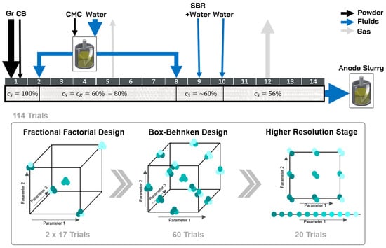
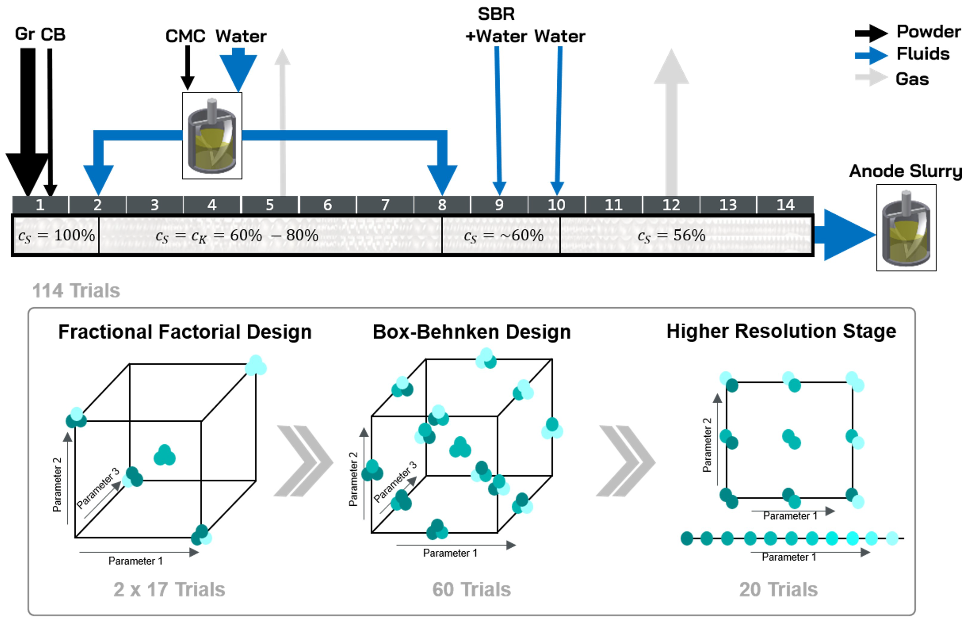
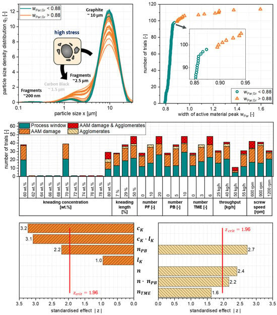
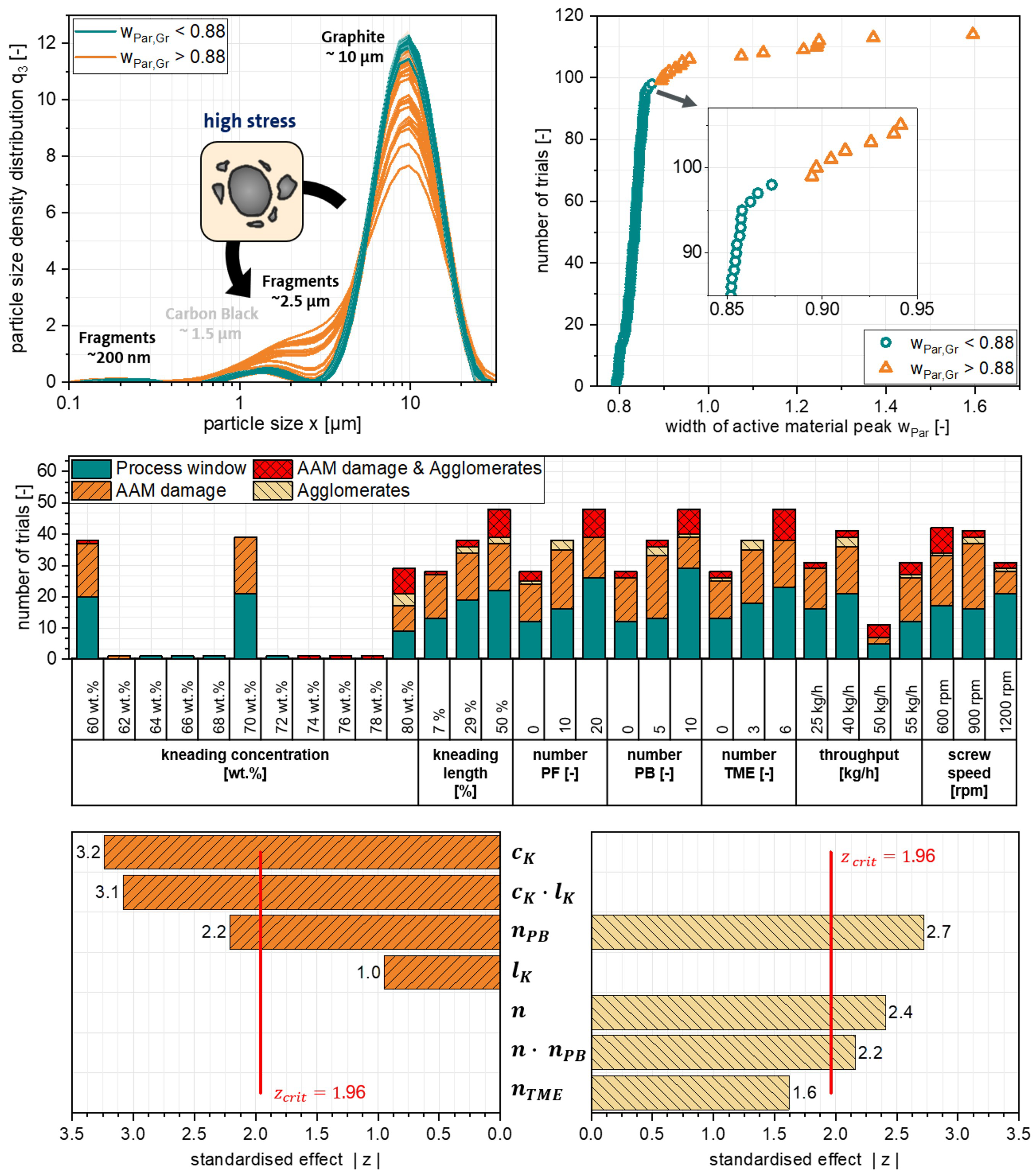
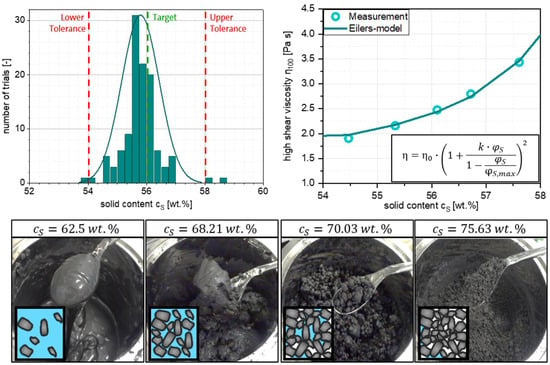
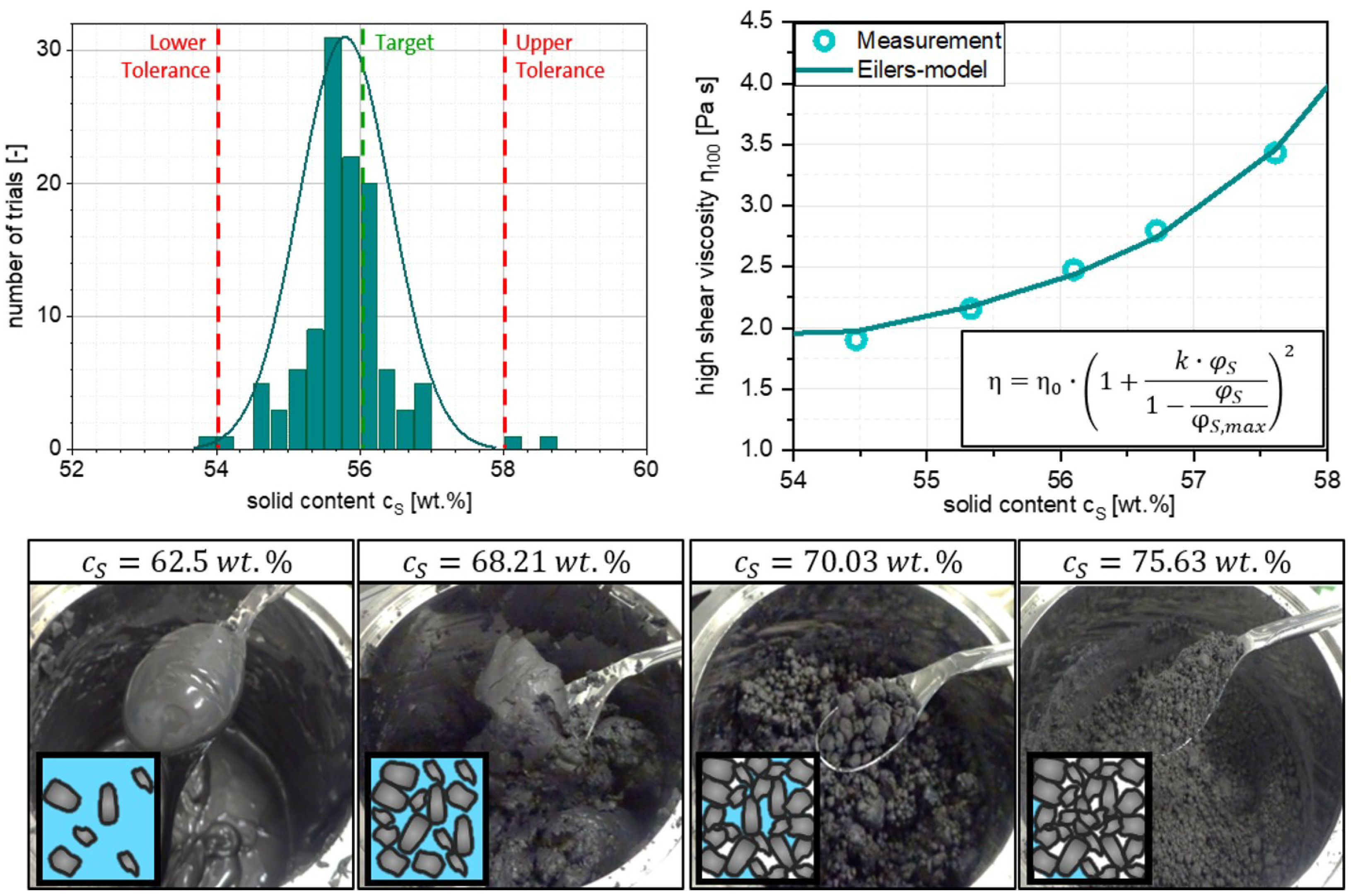
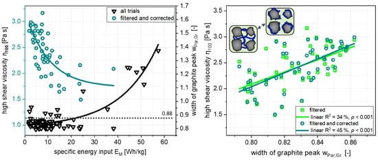
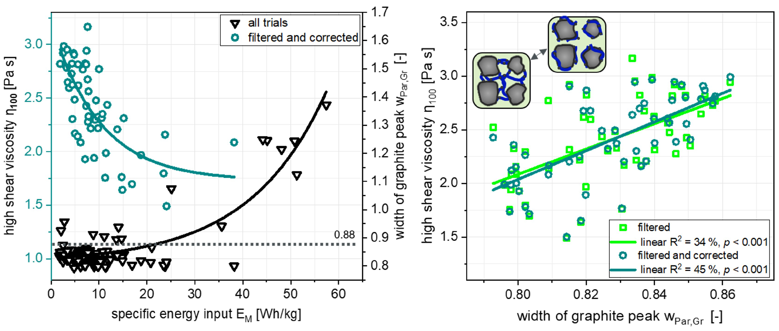
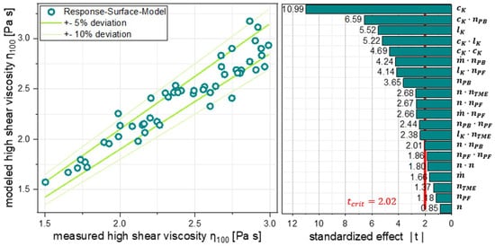
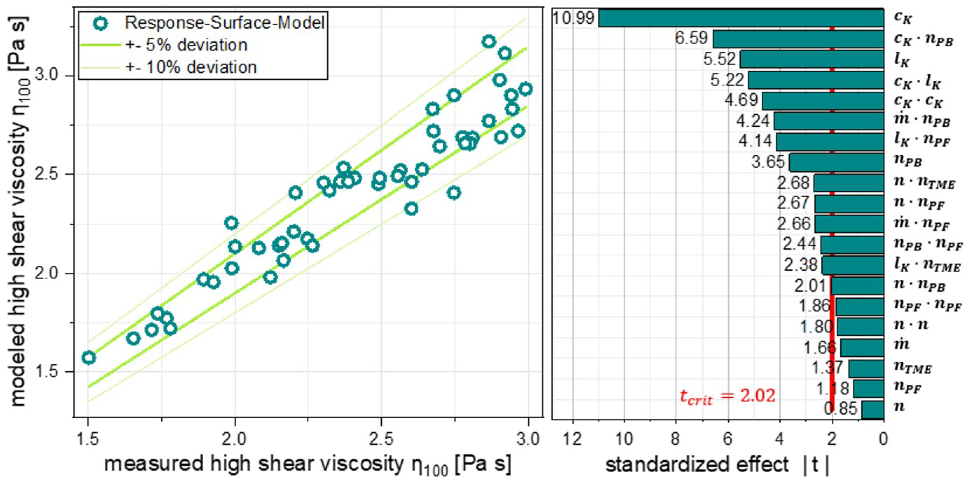
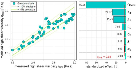
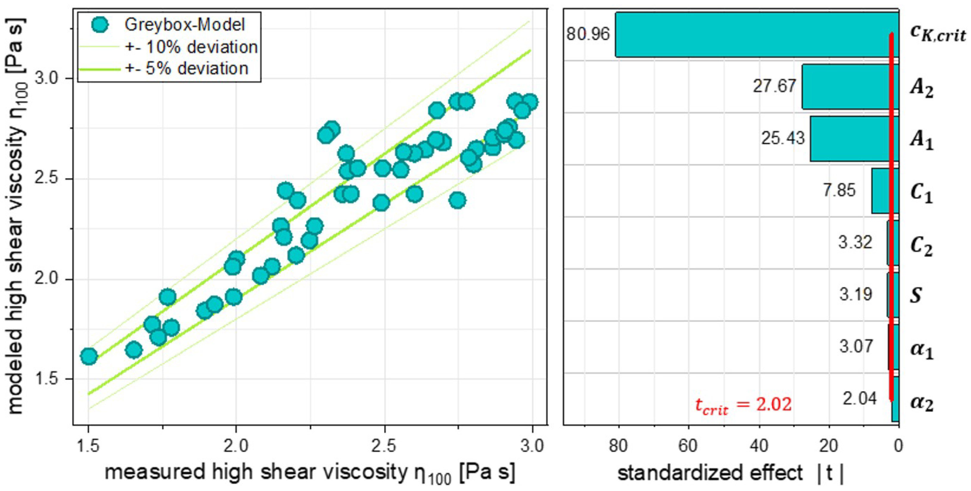
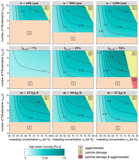
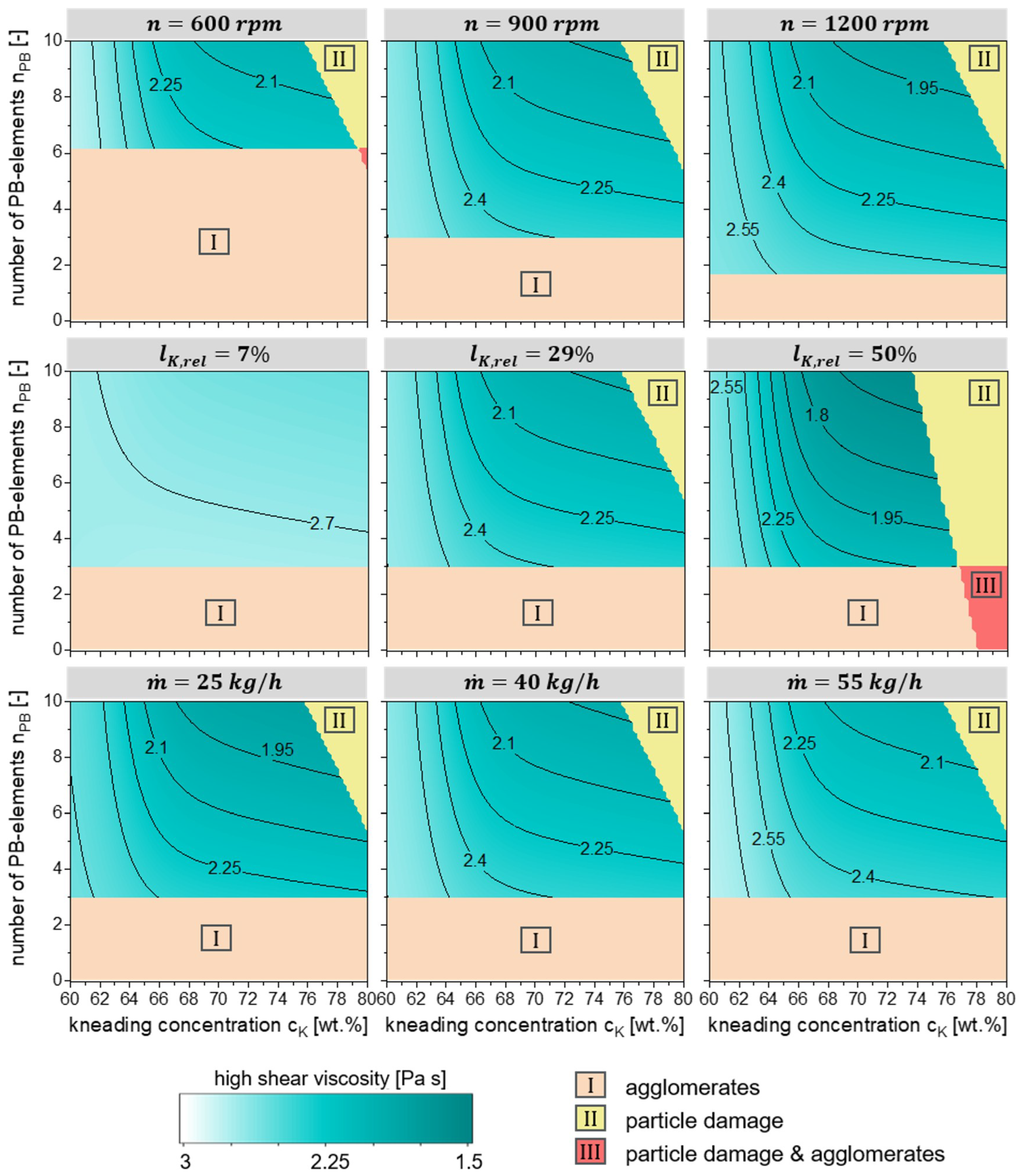

Disclaimer/Publisher’s Note: The statements, opinions and data contained in all publications are solely those of the individual author(s) and contributor(s) and not of MDPI and/or the editor(s). MDPI and/or the editor(s) disclaim responsibility for any injury to people or property resulting from any ideas, methods, instructions or products referred to in the content. |
© 2026 by the authors. Licensee MDPI, Basel, Switzerland. This article is an open access article distributed under the terms and conditions of the Creative Commons Attribution (CC BY) license.