


Abstract
Few-shot adaptation of vision–language models (VLMs) could reduce the labeling effort for defect screening in scanning electron microscopy (SEM) of polymer electrolyte membrane (PEM) fuel-cell materials. We built a leakage-controlled benchmark from the PEMDefect-1107 corpus to measure what VLM language priors contribute. Its controls (size-matched crops, grouping of augmented copies, validation-only selection, common calibration, 20 support draws, image-level bootstrap) were needed: with naive crops, five low-level statistics separated the classes with an area under the receiver operating characteristic curve (AUROC) of 0.951. Zero-shot prompting reached at most 0.685 Macro-F1. With 16 labeled patches per class, text-initialized adaptation of CLIP ViT-L/14 reached 0.823 and, relative to a linear probe on the same features, reduced the labels needed to reach 95% of a fine-tuned ResNet-50 from 512 to 32 per class. A linear probe on ImageNet ResNet-50 features did not differ significantly from it at any tested label budget (difference at 16 shots −0.005; 95% confidence interval −0.059 to 0.044), and two microscopy-pretrained encoders were weaker. On whole micrographs, the better 16-shot classifiers placed 55–63% of the defects in the top 10% of the area. Within each VLM, the text prototypes raised the mean AUROC but gave no detectable advantage over a strong generic encoder.
1. Introduction
Polymer electrolyte membrane (PEM) fuel cells convert hydrogen and oxygen into electricity with water as the only reaction product, and stack lifetime depends on the physical integrity of the membrane, catalyst layer, and gas-diffusion media [1,2]. Membrane durability is tied to the chemistry and structure of the material. For sulfonated poly(ether ether ketone) membranes, the degree of sulfonation trades proton conductivity against swelling and chemical stability in Fenton tests [3], and fluorinated graphite fillers that regulate the membrane microstructure reduce swelling and improve oxidative stability [4]. Perfluorosulfonic acid (PFSA) membranes cast from different resins differ in water uptake, tensile strength, and oxidative stability [5]. Local defects such as pinholes and cracks allow reactant crossover and are a recognized failure mode of membranes [1], so their detection is part of assessing membrane quality and lifetime. Scanning electron microscopy (SEM) is the standard tool for inspecting these components for cracks, pinholes, and other morphological defects. Automated inspection of PEM materials is a recent topic: Yan et al. [6] detected scratches, pinholes, and scuffs in optical images of PEM materials with unsupervised anomaly detection and Faster R-CNN, and a review of 129 studies on computer vision for fuel-cell defect detection identified the lack of standardized benchmarks as the main obstacle to progress [7]. The PEMDefect-1107 corpus, which provides SEM micrographs with defect boxes and fixed splits, was released to address this gap [8]. Annotation remains the limiting step, because defects must be labeled by experts for each new material system and imaging setup.
Vision–language models (VLMs) such as CLIP align images with free-text descriptions at web scale [9,10,11,12], and SigLIP replaces the contrastive softmax objective with a pairwise sigmoid loss [13]; both use the Vision Transformer (ViT) as the image encoder [14]. With such models, a defect class can in principle be specified in words instead of through labeled crops, and a few labeled examples can be used to adapt the frozen model: soft-prompt methods learn continuous prompt tokens [15,16,17], CLIP-Adapter and Tip-Adapter add a residual module or a training-free cache on top of frozen features [18,19], low-rank adaptation reduces the cost of fine-tuning [20], and WiSE-FT interpolates between zero-shot and fine-tuned weights [21]. For industrial inspection, WinCLIP and AnomalyCLIP use CLIP-style prompts to detect and localize anomalies in object images [22,23].
Two recent studies questioned how much of the reported gains of few-shot VLM adaptation survive careful evaluation. Silva-Rodríguez et al. [24] showed that a linear probe initialized at the text embeddings is a strong baseline and that many adaptation methods depend on hyperparameters tuned on large labeled validation sets, which are not available in a genuine few-shot setting; Huang et al. [25] reached a similar conclusion with a linear probe whose weights are blended with the text embeddings. Both studies used natural-image benchmarks. Whether their conclusions transfer to grayscale micrographs, which differ markedly from the web images used for pretraining, is not known, and microscopy-specific pretraining [26] offers a competing source of prior knowledge.
The answer to this question also depends on how the benchmark is built. Few-shot results vary with the examples drawn into the support set, so a single draw can reverse a ranking. Classifiers can exploit shortcuts, that is, cues correlated with the label in a given dataset but unrelated to the property of interest [27]; in patch benchmarks built from detection boxes, crop size and resampling are obvious candidates, and augmented copies of the same micrograph can leak between splits. Selecting backbones or prompts on the test set inflates reported scores. Confidence estimates are often miscalibrated [28], and expected calibration error (ECE) [29] is a biased estimator on small test sets, so it should be complemented by proper scoring rules such as the Brier score and the negative log-likelihood [30,31]. Synthetic image corruptions measure robustness to those corruptions, which is not the same as robustness to a change of acquisition conditions [32].
Previous automated inspection of PEM materials relied on detectors or anomaly detectors trained on images of the target material [6]. To our knowledge, few-shot adaptation of VLMs has not been evaluated on PEM SEM micrographs, and the natural-image studies that questioned few-shot VLM gains [24,25] did not compare VLMs with vision-only encoders under one protocol. This study does not propose a new adaptation method; its contributions concern evaluation. First, it describes a leakage-controlled protocol for turning a detection corpus with an augmented training set into a few-shot classification benchmark (size-matched crops, grouping by base micrograph, validation-only selection, a common calibration protocol, 20 support draws, and image-level bootstrap intervals) and quantifies how these controls change the results. Second, it uses the benchmark to measure what language priors add for PEM SEM defect screening. Zero-shot prompting, including a WinCLIP-style prompt ensemble, and five few-shot methods on three CLIP/SigLIP backbones are compared with DINOv2, ImageNet-pretrained and microscopy-pretrained ResNet-50 encoders, hand-crafted features, and supervised fine-tuning. The results are expressed as the number of labels needed and as whole-micrograph screening performance. Third, the patch index, per-draw results, and analysis code are released for reuse. Section 2 describes the benchmark and methods, Section 3 reports the results, and Section 4 and Section 5 discuss and summarize them.
2. Materials and Methods
2.1. Dataset and Image Grouping
PEMDefect-1107 [8] contains SEM micrographs of PEM fuel-cell materials with YOLO-format bounding boxes around defects, divided into official training (1045 files), validation (31), and test (31) partitions. According to the dataset description, 206 unique micrographs were split before augmentation, and only the training images were expanded with brightness, contrast, and gamma changes within , mild Gaussian noise, light blur, and rotations by multiples of [8]. The training files are therefore augmented copies of 144 base micrographs (file stems ending in _augNNN or _orig). Although the corpus is described as grayscale, about one-third of the training files contain color, whereas all validation and test images are grayscale. We therefore converted every image to grayscale and treated the base micrograph, not the file, as the unit for splitting and resampling. The corpus does not report the instrument, accelerating voltage, magnification, or pixel size of the micrographs, so these settings cannot be given here; the scale-bar region was removed by the preprocessing of the corpus [8], and the figures therefore carry no scale bars.
Our validation split consists of 20% of the training base images, stratified by image series; it is used only for model selection and calibration. The remaining training base images form the support pool from which few-shot examples are drawn. Because the validation split already comes from training images, the official validation and test images together form our test set. Table 1 lists the resulting counts.
Table 1.
Patch counts of the main protocol. Each defective patch has one intact patch of identical size. Images: base images (support pool, validation) or micrographs (test) that contribute at least one pair; 123 of the 144 training base images and 58 of the 62 official validation and test micrographs do; two further test micrographs supply intact patches only. The full patch index is given in Table S1.
Three rules keep information from the test images out of model fitting and selection. Augmented copies of a micrograph share its base image and therefore always fall into the same split; the support pool and the validation split are disjoint sets of base images; and the test images, which were never augmented, are used only for the final evaluation. Because consecutive file numbers in the corpus indicate acquisition sequences, we also audited the official splits for near-duplicate scenes. Every official validation or test micrograph was compared with every training file by the correlation of z-scored gray levels at pixels (best of the eight rotations and flips). A pair was flagged when this correlation was at least 0.90 and the two files were frames of the same sequence whose numbers differ by at most two; both thresholds were set after visual inspection of the 16 highest-scoring pairs (Figure S1; the flagged pairs are listed in Table S6). Nine of the 62 official validation and test micrographs (17 of the 230 test patches) were flagged; each depicts the same scene as one of ten training base images. No such pair exists between the support pool and our validation split. The integrity checks reported with the corpus operate on files [8]; adjacent frames of the same scene are not covered by them. We keep the official split for comparability with other work on the corpus and report the effect of these scenes in Section 3.10, together with a broader criterion that flags every test micrograph with a correlation of at least 0.90, regardless of file name.
2.2. Patch Construction with Matched Geometry
Each defective patch is a square centered on its annotated box, with side length pixels, shifted where necessary to lie inside the image. For each defective patch, one intact patch of exactly the same side length is sampled uniformly from positions in the same micrograph that do not touch any annotated box expanded by 4 pixels. If no such position exists after 400 attempts, the intact square is drawn from another image of the same series and role, with augmented copies of the same base image tried first; this applied to 11.2% of the pairs. Pairs for which no defect-free square of the required size exists anywhere were excluded: 208 of 2617 boxes (7.9%), mostly very large defects with a median square side of 474 pixels. The remaining 2409 pairs give 4818 patches. All patches are converted to grayscale and resized to pixels with bilinear interpolation, so both classes undergo identical scaling. The procedure is deterministic (fixed random seed, no hash-dependent seeding). Figure 1 shows examples.
Figure 1.
Patch construction. (a) Test micrograph with defective (red) and size-matched intact (green) squares. (b) Defective patches. (c) Intact patches of the same side length. (d) The defective patches after the synthetic acquisition perturbation.
To measure shortcut cues, we trained a logistic regression model on the support pool using either crop geometry (width, height, aspect ratio, and relative position) or five low-level statistics of the rendering (mean, standard deviation, variance of an edge-filtered image, mean gradient magnitude, and intensity entropy), and evaluated it on the test patches. The same check was applied to a naive protocol used in our preliminary experiments, in which intact patches were fixed squares and defective patches followed the box shape.
2.3. Distribution-Shift Conditions
Two conditions were evaluated. The synthetic acquisition perturbation applies to each test patch a contrast factor drawn from , a brightness factor from , Gaussian blur with radius pixels with probability 0.75, and additive single-channel Gaussian noise with standard deviation gray levels. Five independent realizations were generated, and results are averaged over them (Figure 1d). The perturbation is a controlled corruption [32]; it does not reproduce a change of microscope, and its operations overlap with the photometric augmentations already applied to the training images [8]. The parameter ranges were set before the experiments and were not derived from multi-instrument data, which are not available for these materials. To place them in context, we measured the brightness (mean gray level), contrast (standard deviation), noise level (estimator of Immerkær [33]), and sharpness (mean gradient magnitude) of the 230 test patches before and after the perturbation (Section 3.9).
The cross-series shift uses a natural partition of the corpus. File names identify image series; the largest series (“nav”) supplies the support pool (2468 patches from its training base images), the validation split (896 patches), and the source test set (192 patches from 44 official validation and test images). The target set contains all other series: their official validation and test images plus one rendering of each of their training base images, which are never used for support in this protocol (176 patches, 44 images).
2.4. Representations
Three VLM image–text encoders were used through OpenCLIP [11]: CLIP ViT-B/16 and ViT-L/14 [9] and SigLIP ViT-B/16 [13]. Two vision-only encoders were taken from the timm library [34]: DINOv2 ViT-B/14 [35] and an ImageNet-1k (IN-1k) ResNet-50 [36] trained with the recipe of Wightman et al. [37]. Two microscopy-pretrained ResNet-50 encoders were added from the MicroNet release [26], a collection of more than 100,000 labeled micrographs: one trained from scratch on MicroNet and one initialized on ImageNet and fine-tuned on MicroNet (weights v1.1 and v1.0 of the release, respectively; inputs normalized with the MicroNet channel statistics). The encoders were chosen to separate sources of prior knowledge: language supervision (the two most widely used CLIP checkpoints and SigLIP, which uses a different training loss), self-supervised learning on natural images (DINOv2), supervised ImageNet classification (ResNet-50), and supervised pretraining on micrographs (MicroNet). The MicroNet encoders share the ResNet-50 architecture of the ImageNet encoder, so this comparison isolates the effect of the pretraining data. All encoders are frozen; image features are L2-normalized. As a reference without deep features, the five low-level statistics of Section 2.2, standardized with the mean and standard deviation of the unlabeled support pool, were also used as a representation.
2.5. Zero-Shot Classification
For a VLM with image encoder and text encoder , the prototype of class c is the normalized mean of the normalized embeddings of J prompt templates ,
and a patch with normalized image embedding receives logits , where is the model’s learned logit scale. Probabilities are obtained with a softmax over the two classes; for SigLIP, the learned logit bias is the same for both classes and cancels in the softmax. Table 2 lists the prompt families. Each family was combined with a long, descriptive class phrase and with a short one. As a zero-shot baseline from industrial anomaly detection, we also implemented a WinCLIP-style compositional prompt ensemble [22]: seven normal-state phrases (e.g., “flawless {}”, “{} without defect”) and five anomalous ones (e.g., “damaged {}”, “{} with flaw”), each combined with twelve templates and the object word “membrane surface”. Patches were scored either with the whole-patch embedding or with the mean of the whole-patch probability and the maximum over nine half-size sub-windows, a simplified form of WinCLIP’s window aggregation (our re-implementation; the original code was not used).
Table 2.
Prompt templates and class phrases. {} is replaced by the class phrase.
2.6. Few-Shot Methods
A support set contains labeled patches per class. Five methods were compared; the last three require a VLM because they use the text prototypes (domain templates, long phrases).
Linear probe (LP). -regularized logistic regression on the frozen features (scikit-learn, ).
Nearest class mean (NCM). Logits , where is the normalized mean of the support features of class c ( for vision-only encoders).
Tip-Adapter [19]. With support features and one-hot labels , the logits are
with and ; no parameters are trained.
Prototype residual tuning (PRT). The text prototypes are corrected by a learned residual,
where (initialized at zero) and the scalar s (initialized at 0.1) are optimized by full-batch AdamW (learning rate 0.005, weight decay 0.01) for 140 steps when and 220 steps otherwise, minimizing cross-entropy on . We avoid the term “prompt” for this mechanism because it changes the class prototypes in embedding space and learns no prompt tokens.
Text-initialized linear probe (TI-LP). A linear classifier with weights , obtained by minimizing
with L-BFGS, . It is the convex counterpart of PRT and isolates the effect of initializing a linear classifier at the text prototypes.
These settings form the default regime and were fixed before any results were seen; they are the same for every representation, so no method was adapted to the test data. In a second, tuned regime, hyperparameters were additionally selected on the validation split from the grids ; and ; PRT learning rate and steps ; ; and, for the text-based methods, generic or domain templates. The grids differ in size between methods because the methods have different hyperparameters, but every method is selected with the same validation split, criterion, and support draws.
Two reference models use all labels of the support pool: a full-data linear probe on each representation (C selected on validation) and supervised fine-tuning of the ResNet-50 end to end (AdamW, learning rate , weight decay 0.05, cosine schedule, 15 epochs, batch size 64, random flips and rotations, epoch selected on validation Macro-F1; three seeds).
2.7. Evaluation Protocol and Statistics
For each k and each of the 20 support draws, the support set is drawn from k distinct base images per class, with one random patch per base image, so that augmented copies of one micrograph never appear twice in a support set. All methods and representations share the same draws.
Selection. For every method and k, the representation (and, for zero-shot classification, the prompt family and class phrase) with the highest mean validation Macro-F1 over the 20 draws is selected; ties are broken by lower validation ECE. No test information enters this step. Selection uses the labeled validation split (1170 patches), and calibration uses 64 of its labels; these labels are not counted in k. The results for a fixed representation with default settings do not depend on this selection.
Calibration. Every method, including zero-shot classification, is temperature-scaled [28] with the same budget: for each seed, 32 validation patches per class are drawn and the temperature T minimizing their negative log-likelihood is found by bounded scalar optimization over . Results are reported with and without calibration; the uncalibrated zero-shot classifier uses no labels at all.
Metrics. Macro-F1 (the unweighted mean of the F1 scores of the two classes) is the primary metric. Calibration is measured by ECE with 15 equal-width bins [29], ECE with 15 equal-mass bins [31], the Brier score [30], and the negative log-likelihood (NLL), using the maximum class probability as confidence. Because binned ECE is sensitive to the bin boundaries on a test set of 230 patches, we also report the binning-free Kolmogorov–Smirnov (KS) calibration error [38], the maximum absolute difference between the normalized cumulative sums of confidence and accuracy over patches sorted by confidence, ECE with 5 to 30 bins, and cluster-bootstrap intervals of both.
Uncertainty. Test patches are not independent: several pairs come from the same micrograph. Confidence intervals are therefore obtained with a cluster bootstrap [39] that resamples test micrographs (2000 resamples, each pair kept with the image of its defective patch); within each resample, metrics are averaged over the 20 draws (and, for perturbed images, the five realizations), and 95% percentile intervals are reported. These intervals describe the sampling of test images; they are conditional on the 20 support draws and on the composition of the support pool. Differences between methods are computed on the same resamples. For source–target differences, an equivalence margin of Macro-F1 was fixed before the analysis and assessed with the 90% interval, which corresponds to two one-sided tests at the 5% level [40].
Label cost. To estimate how many labels are needed, the default-setting methods were also evaluated for with ten draws each; when k exceeds the number of base images of a class, every base image is used once and the remainder is drawn from the other patches of the pool. We report the smallest k at which the mean test Macro-F1 reaches 90% and 95% of the fine-tuned ResNet-50 (Section 2.6); the result is resolved only to the tested values of k.
Whole-micrograph screening. To assess the classifiers as inspection tools, all 62 official validation and test micrographs were covered with non-overlapping tiles of and pixels, rendered exactly like the patches. A tile is positive if it contains the center of an annotated box whose longer side does not exceed the tile, negative if it does not touch any box expanded by 4 pixels, and ambiguous otherwise. Classifiers trained on support patches per class (20 draws, probabilities averaged) score every tile; we report the tile-level area under the receiver operating characteristic curve (AUROC) and average precision, and the fraction of all annotated defects whose center falls in the top 5%, 10%, or 20% of tiles of their micrograph, i.e., the defects an inspector would see after examining that fraction of the image area. A random ranking finds, on average, the same fraction of defects as of area. Because this center-based recall counts large and small defects equally, we also report an area-weighted recall (the fraction of the total annotated box area covered by the selected tiles), a coverage recall (the fraction of boxes with at least 50% of their area covered), and the center recall separately for boxes whose longer side is below 32 pixels, 32–96 pixels, and above 96 pixels. An oracle that ranks tiles by the true fraction of defect area they contain gives the upper bound of the area-weighted recall at a given budget and a reference value for the other metrics.
Near-duplicate sensitivity. The selected configurations, zero-shot classification, the full-data probe, and the ResNet-50 classifiers were re-evaluated (A) without the nine flagged test micrographs, (B) with the ten flagged training base images removed from the support pool and validation split, and (C) with both changes.
Software. Features were extracted once with Python 3.10.11, PyTorch 2.5.1, OpenCLIP 3.3.0, and timm 1.0.20 on an NVIDIA GeForce RTX 2070 SUPER (NVIDIA Corporation, Santa Clara, CA, USA); all few-shot methods, calibration, and statistics were computed from the stored features with NumPy 2.2.6, SciPy 1.15.3, pandas 2.3.3, and scikit-learn 1.7.2. Per-draw results are given in Tables S2 and S3, and the code with its run order in Code S1. PRT was re-implemented in NumPy with analytic gradients, which were checked against finite differences.
2.8. Diagnostic Analyses
Background context. To test whether the classes can be told apart from the surroundings of a defect rather than from the defect itself, every patch was also rendered in two masked forms (Figure 2). In the object-only form, all pixels outside the annotated box are replaced by the mean gray level inside the box; in the context-only form, the box (dilated by 2 pixels) is replaced by the mean gray level of the surrounding ring. The paired intact patch receives the same box (box geometry in Table S5), so masking removes the same area from both classes. The box covers a median of 59% of the patch area. The five low-level statistics and all deep representations were recomputed for both forms, and linear probes were trained and tested on the same form. As a measure of spatial autocorrelation, we computed the correlation length of the gray levels (the lag at which the radially averaged autocorrelation drops below ) and Moran’s I with four-neighbor weights on eightfold-downsampled test patches.
Figure 2.
Masked renderings used for the background-context control. Columns: original patch, object-only (pixels outside the annotated box replaced by the mean gray level of the box), and context-only (box replaced by the mean gray level of the surrounding ring). Defective patches alternate with their size-matched intact partners, which are masked with the same box.
Text–image alignment. For each VLM, the text direction (domain templates, long phrases) was compared with the image features in three ways: the mean cosine between image embeddings and each text prototype, the test AUROC of the projection of the image embeddings on the text direction (the zero-shot score), and the cosine between the text direction and the weight vector of a linear probe trained on all 3418 support-pool patches. The same cosine was computed for the weight vectors of the few-shot LP and TI-LP. Test AUROC, which does not depend on the decision threshold, was computed for LP and TI-LP at and .
Representation analysis. For every representation we computed a class-separation ratio on the support pool (squared distance between the class means divided by the mean within-class variance), the participation ratio of the within-class covariance as a measure of effective dimensionality, and linear centered kernel alignment (CKA) [41] between encoders on the validation and test patches. To locate where the MicroNet encoders lose information, linear probes were also trained on the globally average-pooled outputs of the four residual stages (layer1 to layer4) of the three ResNet-50 encoders.
3. Results
Unless stated otherwise, results refer to the main protocol and to the original (unperturbed) test images; few-shot values are means over 20 support draws, and bracketed ranges are 95% cluster-bootstrap intervals.
3.1. Shortcut Controls
Table 3 shows that the naive patch protocol leaked label information through the crop itself. Crop geometry alone separated the classes with an AUROC of 0.696, and five low-level statistics reached an AUROC of 0.951. With matched geometry, the width, height, and aspect ratio are identical within each pair; the remaining geometric signal (AUROC 0.616) comes from position, because 12.2% of the defective squares touch the image border compared with 1.9% of the intact squares, and position is not visible in the crop content. The low-level statistics still reach an AUROC of 0.863, which reflects real differences in contrast and texture between defective and intact regions. We therefore treat the low-level statistics as a baseline representation that every learned method should exceed.
Table 3.
Shortcut controls: logistic regression trained on the support pool and evaluated on the test patches, using crop geometry or five low-level image statistics only.
The masked renderings show where this signal lies (Table 4). With the defect box replaced by a uniform gray value, the low-level statistics separated the classes with an AUROC of only 0.567, and linear probes on every deep representation reached a test AUROC of 0.526–0.585 at and 0.606–0.730 with all labels. With only the box retained, performance was similar to or higher than on the original patches (low-level statistics 0.889; deep representations 0.827–0.922 at ). Most of the class information, both in the low-level statistics and in the deep features, is therefore inside the annotated box. The remaining context signal with all labels is consistent with the local texture around a defect, but it is small compared with the signal of the defect itself. This control has two limits: the context ring is narrow (about 18 pixels of the rendering along the longer box side), so only the immediate surroundings of a defect are tested, and the uniform fill creates an input unlike the training images. The object-only renderings, which contain the same kind of fill, kept their accuracy, so the fill alone does not explain the low context-only scores. The gray levels were spatially autocorrelated over short distances only. In intact test patches, the correlation length had a median of 8 pixels of the rendering (interquartile range 4–17 pixels; Moran’s I 0.66), shorter than the width of the context ring (about 18 pixels) in 72% of the patches, and the mean gray level of the ring and of the box region correlated almost perfectly across intact patches (). In defective patches the correlation length was longer (median 26 pixels; Moran’s I 0.88), because the defect is a large coherent structure, and the ring predicted the box less well ().
3.2. Zero-Shot Classification and Prompt Wording
Zero-shot Macro-F1 ranged from chance level to 0.685 depending on backbone, templates, and class phrase (Table 5). The short class phrases (“intact surface”, “defective surface”) failed with every backbone (at most 0.406 in Table 5, and 0.505 for one individual domain template); several combinations assigned all patches to one class (Macro-F1 ). With the long phrases, no template family was consistently better: domain templates improved CLIP ViT-L/14 (0.676 versus 0.512 for one generic template) but degraded CLIP ViT-B/16 (0.457 versus 0.685). The configuration selected on validation, CLIP ViT-B/16 with one generic template and the long phrases, reached 0.685 [0.570, 0.779] on the test images.
Table 5.
Zero-shot Macro-F1 on the original test images for each backbone, template family, and class phrase. † Configuration selected on the validation split.
The WinCLIP-style prompt ensemble did not outperform the class-phrase prompts overall (Table 6). On the CLIP backbones its patch-level AUROC (0.619–0.666) was below that of the class phrases (0.680–0.762). On SigLIP its AUROC was slightly higher (0.770–0.788 versus 0.742–0.769), but its Macro-F1 (0.556–0.595) was below that of the class phrase with the generic template (0.679). Adding sub-window scores changed AUROC by at most 0.039. In this test, generic anomaly vocabulary (“damaged”, “with flaw”) was not a better description of PEM SEM defects than a descriptive class phrase.
Table 6.
Zero-shot scoring of the original test patches with class-phrase prompts and with a WinCLIP-style compositional prompt ensemble (our re-implementation). Macro-F1 uses the arg-max decision.
3.3. Few-Shot Learning Curves
Table 7 and Figure 3 give the test Macro-F1 of each few-shot method as a function of k. All methods improved with k, and at the two text-initialized methods on CLIP ViT-L/14 scored highest (PRT 0.823 [0.769, 0.870]; TI-LP 0.817 [0.763, 0.863]). PRT exceeded Tip-Adapter by 0.031 [0.010, 0.049] and did not differ significantly from TI-LP (0.006 [−0.003, 0.013]), which suggests that the benefit comes from initializing the classifier at the text prototypes rather than from the particular optimizer. Draw-to-draw variability was largest at small k: the standard deviation over draws of the linear probe was 0.088 at , and at the worst individual draws of the linear probe, NCM, PRT, and TI-LP reached 0.48–0.62 Macro-F1 and the best 0.80–0.87. Tip-Adapter was the most stable method (standard deviation 0.017–0.022 at all k; range 0.654–0.745 at ).
Table 7.
Test Macro-F1 (mean ± standard deviation over 20 support draws) of the validation-selected configuration of each method. The backbone was selected separately for each k; the backbone selected at is shown, and at SigLIP ViT-B/16 was selected for LP, NCM, PRT, and TI-LP.
Figure 3.
Macro-F1 versus the number of labeled patches per class for the validation-selected configuration of each method. (a) Original test images of the main protocol. (b) Target series of the cross-series protocol. Lines are means over 20 support draws; shaded bands span the 2.5th to 97.5th percentiles of the draws. Horizontal lines mark the selected zero-shot classifier, the full-data linear probe, and the fine-tuned ResNet-50.
Table 8 separates the effect of the representation from that of the method at . Within each VLM, the text-initialized methods outperformed a linear probe on the same features at and ; on CLIP ViT-L/14 the difference was 0.075 [0.055, 0.094] at , 0.009 [−0.001, 0.021] at , and 0.032 [0.013, 0.059] at , and on SigLIP ViT-B/16 it was 0.034 [0.012, 0.053] at and 0.047 [0.017, 0.078] at (Table 9). Across representations, the text-based methods held no advantage. At , a linear probe on the ImageNet ResNet-50 reached 0.827 and NCM on the same features 0.834, and PRT on CLIP ViT-L/14 did not differ significantly from either at any tested k; all intervals include zero (at : −0.005 [−0.059, 0.044] and −0.013 [−0.067, 0.036]). Because the validation split favored DINOv2 for the linear probe, the selected linear probe (0.770) understates the test performance of the best vision-only features. The two MicroNet encoders reached 0.737 and 0.716 with a linear probe at , below the ImageNet ResNet-50 of the same architecture (0.827). The layer-wise probes locate the difference (Table 10). In the first two residual stages, the MicroNet features were at least as informative as the ImageNet features (layer1: AUROC 0.733 versus 0.631 at ; full-data Macro-F1 0.830 versus 0.754). From layer2 to layer4, the ImageNet features improved steadily (to 0.900 and 0.921), whereas the MicroNet features improved little in AUROC (0.766 to 0.825) and not at all in full-data Macro-F1 (0.825 to 0.797), and for the ImageNet → MicroNet encoder the final stage was worse than layer3 (0.834 versus 0.846 at ). Restricting the input to the defect box raised the MicroNet probes from 0.825 to 0.866 (AUROC, ; Table 4), more than for the ImageNet ResNet-50 (0.900 to 0.916). The class-separation ratio on the support pool was 0.389 for MicroNet, 0.333 for the ImageNet ResNet-50, and 0.178 for ImageNet → MicroNet, and the linear CKA between the final ImageNet and MicroNet features was 0.57–0.60, lower than between the ImageNet ResNet-50 and DINOv2 (0.65) or CLIP ViT-L/14 (0.64).
Table 8.
Test Macro-F1 at (default settings, mean ± standard deviation over 20 draws) for every representation and method. Text-based methods require a VLM.
Table 9.
Paired differences in test Macro-F1 between a text-initialized method and a feature-based classifier (same support draws, same bootstrap resamples).
Table 10.
Layer-wise linear probes of the three ResNet-50 encoders (globally average-pooled outputs of each residual stage): test AUROC at (mean of 20 draws)/test Macro-F1 of the full-data probe.
3.4. Text–Image Alignment
Image and text embeddings were weakly aligned (Table 11). The mean cosine between test image embeddings and the two text prototypes was 0.23–0.28 for the CLIP models and 0.03–0.04 for SigLIP, and it differed by at most 0.010 between the intact and the defect prototype. The text direction was almost orthogonal to the weight vector of a linear probe trained on all support-pool patches (cosine 0.071–0.097, against an expected absolute cosine of 0.035 and 0.029 for random directions in the 512- and 768-dimensional spaces), yet projecting the test images on it ranked defective above intact patches with an AUROC of 0.742–0.759. Figure 4a shows the consequence for CLIP ViT-L/14: the two classes overlap along the text direction and separate along the data-derived direction. Few-shot linear probes approached the data-derived direction quickly (cosine 0.33–0.36 at and 0.61–0.70 at ), whereas TI-LP stayed farther from it (0.18–0.20 and 0.36–0.47) because its weights remain anchored at the text prototypes. Nevertheless, TI-LP ranked the test patches better than LP on the same features in five of the six comparisons (Figure 4b): at , test AUROC rose from 0.830 to 0.878 on CLIP ViT-B/16, from 0.894 to 0.907 on CLIP ViT-L/14, and from 0.849 to 0.860 on SigLIP; at SigLIP was the exception (0.800 versus 0.793). Paired cluster-bootstrap intervals of the difference excluded zero in three of the six comparisons: CLIP ViT-B/16 at (+0.043 [0.016, 0.076]) and (+0.048 [0.027, 0.072]), and CLIP ViT-L/14 at (+0.028 [0.001, 0.055]). A linear probe on ImageNet ResNet-50 features reached 0.731 at and 0.900 at without any text.
Table 11.
Text–image alignment on the original test images. cos(image, intact/defect): mean cosine between image embeddings and the two text prototypes. Ref.: weight vector of a linear probe trained on all 3418 support-pool patches. Few-shot directions and AUROC are means over 20 support draws; text dir.: zero-shot score (projection on ).
Figure 4.
Text–image alignment. (a) Test patches of CLIP ViT-L/14 projected on the normalized text direction (horizontal) and on the component of the full-data linear-probe direction orthogonal to it (vertical). (b) Test AUROC of the zero-shot text direction and of LP and TI-LP at and (means over 20 draws); ImageNet ResNet-50 shown for reference (LP only).
3.5. Comparison with Full Supervision and Hand-Crafted Features
Few-shot adaptation closed about two-thirds of the gap between zero-shot classification and the full-data probe, and a significant gap to full supervision remained (Table 12). PRT at exceeded the selected zero-shot classifier by 0.138 [0.072, 0.219] and stayed 0.071 [0.021, 0.123] below the full-data linear probe on CLIP ViT-L/14 (0.895), which used all 3418 support-pool patches (Table 13). End-to-end fine-tuning of the ResNet-50 on the same patches reached over three seeds, close to the full-data probe. The low-level statistics reached 0.749 with and 0.811 with all labels; the best few-shot methods, trained on 16 labeled patches per class (32 in total), therefore reached about the same Macro-F1 as a hand-crafted classifier trained on 3418 patches (0.823 versus 0.811; this difference was not tested).
Table 12.
Macro-F1 at and for the full-data references on the source and target test sets of both shift conditions. Few-shot rows use the validation-selected configuration; intervals are 95% cluster-bootstrap intervals; fine-tuning is mean ± standard deviation over three seeds.
Table 13.
Paired differences in Macro-F1 between validation-selected configurations at (zero-shot and full-data references as marked), with 95% cluster-bootstrap intervals.
3.6. Label Cost
Figure 5 and Table 14 extend the learning curves to 512 labeled patches per class and express them as the labels needed to reach 90% and 95% of the fine-tuned ResNet-50 (Macro-F1 0.882). PRT and TI-LP on every VLM, and the linear probe and NCM on the ImageNet ResNet-50, reached 95% with 32 labeled patches per class. A plain linear probe on the same VLM features needed 256–512 patches per class for 95%, so the text initialization reduced the label requirement by a factor of 8–16 within a VLM, but not relative to the ImageNet ResNet-50. NCM and Tip-Adapter saturated below 90% on all VLMs except Tip-Adapter on CLIP ViT-L/14 (90% at ). The MicroNet encoders and the hand-crafted features did not reach 95% within 512 patches per class.
Figure 5.
Test Macro-F1 versus labeled patches per class up to (20 draws for , 10 draws above) for selected representations and methods. Horizontal lines mark 90%, 95%, and 100% of the fine-tuned ResNet-50. Per-draw values are given in Table S3.
Table 14.
Labeled patches per class needed to reach 90% and 95% of the fine-tuned ResNet-50 (Macro-F1 0.882) on the original test images, and the best mean Macro-F1 reached up to (default settings).
3.7. Whole-Micrograph Screening
On tiles of the 62 test micrographs, the classifiers in Table 15, trained with , reached a tile AUROC of 0.846–0.929; across all 26 representation–method combinations (Table S4) the range was 0.815–0.965. Expressed as an inspection budget, examining the 10% highest-scoring tiles of each micrograph would have revealed 39–63% of the 118 annotated defects, against 10% for a random order; inspecting 20% of the area raised this to 53–82%. The ranking of representations differed from that in the patch benchmark. The ImageNet ResNet-50 linear probe found the most defects at a 10% budget (0.627 with tiles), followed by the MicroNet encoders, DINOv2, and SigLIP with TI-LP (0.551–0.585); the text-initialized methods on CLIP ViT-L/14 found 0.390–0.407, although they were the best patch classifiers. Among the configurations in Table 15, SigLIP with TI-LP had the highest tile AUROC (0.928–0.929). The text-based methods on CLIP ViT-B/16, not shown in the table, reached 0.953–0.965 with tiles and a recall of 0.46–0.51 at a 10% budget (Table S4). Without any labels, the WinCLIP-style zero-shot score on SigLIP reached a recall of 0.466 at a 10% budget. With tiles, recall at 10% was 0.36–0.46 for all classifiers in Table 15, because many defects are small relative to the tile and several share one tile.
Table 15.
Whole-micrograph screening of the 62 test micrographs with classifiers trained on patches per class (20 draws, averaged probabilities). Shown are the validation-selected few-shot configurations (CLIP ViT-L/14 for the text-based methods, DINOv2 for LP), the ResNet-50 probes, and two SigLIP configurations; all 26 combinations are listed in Table S4. AUROC is computed over positive and negative tiles; Rec@q is the fraction of the 118 annotated defects whose center lies in the top-q fraction of tiles of their micrograph.
Recall weighted by defect area was lower than center recall (Table 16). At a 10% budget with tiles, the selected tiles covered 18–35% of the annotated defect area and covered at least half of the area of 34–55% of the boxes. These values should be interpreted relative to the oracle: the defects occupy a median of 10.7% of the area of a test micrograph (interquartile range 4.5–24.3%), so even a perfect ranking covers only 41.5% of the defect area and finds 72.9% of the defect centers at this budget. The ImageNet ResNet-50 thus reached 86% of the oracle center recall (0.627 of 0.729) and 77% of the oracle area-weighted recall (0.319 of 0.415). By size, the classifiers found 19–38% of the 21 small defects (longer side below 32 pixels), 57–81% of the 37 medium defects, and 30–62% of the 60 large ones; the text-initialized methods on CLIP ViT-L/14 were weakest on large defects (0.300–0.333), which explains most of their lower overall recall.
Table 16.
Size-aware screening metrics at an inspection budget of 10% of the area ( tiles, 62 test micrographs, 118 annotated defects; classifiers as in Table 15). Center recall: fraction of defects whose center lies in a selected tile. Area-weighted recall: fraction of the total defect area covered. Coverage recall: fraction of defects with at least 50% of their area covered. Size classes by the longer box side: 21 small (<32 px), 37 medium, and 60 large (>96 px) defects. The oracle ranks tiles by their true defect-area fraction. Results for all budgets and tile sizes are given in Table S7.
3.8. Calibration
Without calibration, ECE at ranged from 0.074 (Tip-Adapter) to 0.152 (linear probe on DINOv2) on the original test images (Table 17, Figure 6). The fitted temperatures show that much of this spread is a matter of logit scale: the linear probe was underconfident (median , i.e., its logits had to be sharpened), and PRT was overconfident (median ). After temperature scaling with 64 validation labels, ECE ranged from 0.073 to 0.109 and the Brier score from 0.129 to 0.168 for the few-shot methods, with overlapping intervals; PRT and TI-LP had the lowest Brier score and NLL. Calibration did not help the zero-shot classifier (ECE 0.118 uncalibrated versus 0.131 calibrated), because the temperature fitted on validation patches did not transfer to the test images. In three of the 1042 calibration fits of selected configurations (all in the cross-series protocol at ), the temperature reached the upper search limit, which corresponds to a classifier at chance level on its calibration subset and yields predictions close to 0.5.
Table 17.
Calibration on the original test images at (means over 20 draws). Calibrated values use temperature scaling with 32 validation patches per class; T is the median fitted temperature.
Figure 6.
ECE on the original test images at before and after temperature scaling, with 95% cluster-bootstrap intervals.
The binning-free KS calibration error led to the same conclusions (Table 18). After calibration it was 0.041–0.093 for the few-shot methods, and temperature scaling reduced it for the linear probe (0.139 to 0.081), PRT (0.132 to 0.062), and TI-LP (0.089 to 0.061) but not for NCM, Tip-Adapter, or the zero-shot classifier. The choice of bins mattered: for a given method, ECE varied by 0.026–0.042 between 5 and 30 bins, which is as large as most differences between methods. The cluster-bootstrap intervals were wide (for example 0.042–0.112 for the KS error of PRT) and lay mostly above the point estimates, because resampling with replacement duplicates patches and both estimators are biased upward in small samples. With 230 test patches from 58 micrographs, the calibration comparison can therefore separate well-calibrated from clearly miscalibrated classifiers (e.g., the uncalibrated linear probe), but not rank the calibrated few-shot methods.
Table 18.
Binning-free calibration on the original test images at (means over 20 draws; brackets: 95% cluster-bootstrap intervals, 1000 resamples). KS: Kolmogorov–Smirnov calibration error [38]. ECE range: minimum and maximum of the calibrated ECE over 5, 10, 15, 20, and 30 equal-width bins.
3.9. Distribution Shift
Neither shift condition reduced Macro-F1 (Table 12, Figure 7). Under the synthetic acquisition perturbation, source-minus-target differences ranged from to . For the text-based methods and the full-data probe the 90% intervals were contained in , so a loss larger than 0.034 Macro-F1 can be ruled out at the 5% level; equivalence within the pre-specified margin was not established because the intervals extended beyond the margin, mostly toward better target performance. The linear probe and NCM on DINOv2 improved under perturbation ( [, ] and [, ]). The perturbation kept brightness, contrast, and sharpness within the range of the original test patches: the mean gray level of 95.5% of the perturbed patches, and the standard deviation and mean gradient magnitude of all of them, lay between the minimum and maximum of the originals. It raised the noise level, however, from a median of 0.41 to 13.9 gray levels (Immerkær estimator), above the 95th percentile of the original patches (5.5) for 99.9% of the perturbed patches but below the noisiest original (20.4). The perturbation is therefore a mild photometric change combined with strong noise, not a model of a different instrument.
Figure 7.
Source versus target Macro-F1 at and for the references, with 95% cluster-bootstrap intervals; backbones as in Table 12 (LP and NCM: DINOv2 ViT-B/14; text-based methods and full-data probe: CLIP ViT-L/14; zero-shot: CLIP ViT-B/16). (a) Synthetic acquisition perturbation. (b) Cross-series shift. Points above the dashed identity line perform better on the target.
The cross-series target was easier than the source for every method, including the fine-tuned ResNet-50 ( on the source and on the target, difference ). For the other methods the differences ranged from (full-data probe) to (Tip-Adapter). The intensity statistics suggest one reason: across all patches, the mean standard deviation of gray levels differed more between defective and intact patches in the other series (46.1 versus 18.5) than in the nav series (42.9 versus 22.8), so defects stand out more clearly from their background.
3.10. Sensitivity to Near-Duplicate Scenes
Removing the nine test micrographs that depict the same scene as a training image lowered Macro-F1 by 0.008–0.015 for every configuration (Table 19), so these scenes were slightly easier than the rest of the test set. Removing the ten corresponding base images from the support pool and validation split changed Macro-F1 by to . With both changes, the ranking of the configurations was unchanged: PRT (0.819) and TI-LP (0.812) on CLIP ViT-L/14 remained within 0.013 of the ImageNet ResNet-50 linear probe (0.825) and NCM (0.825), and these four classifiers remained at least 0.14 above zero-shot classification (0.670). With the broader criterion (correlation of at least 0.90 regardless of file name), 14 test micrographs (50 test patches) and 18 training base images were flagged. Removing both lowered Macro-F1 by 0.018–0.057; the four classifiers then reached 0.781–0.806, with the ImageNet ResNet-50 classifiers 0.008–0.025 above the text-initialized ones, and none of the conclusions changed (Supplementary Table S6).
Table 19.
Test Macro-F1 at (20 draws) with the near-duplicate scenes of Section 2.1 removed: (A) nine flagged micrographs (17 patches) removed from the test set; (B) ten flagged base images (82 support and 16 validation patches) removed from the support pool and validation split; (C) both.
3.11. Validation–Test Discrepancy and Hyperparameter Tuning
Validation scores were systematically higher than test scores. At , validation Macro-F1 of the selected configurations was 0.84–0.88, compared with 0.75–0.82 on the test images. The validation split consists of training base images, which share series, preparation, and augmentation history with the support pool, whereas the test images are separately acquired originals. Tuning hyperparameters on this split did not improve test performance: at the tuned regime gave 0.749 for the linear probe (default 0.770), 0.790 for Tip-Adapter (0.791), 0.821 for PRT (0.823), and 0.815 for TI-LP (0.817).
4. Discussion
What the controls changed. Several design choices that are common in patch benchmarks would have changed the conclusions of this study. When defects were cropped along their boxes and intact regions as fixed squares, five low-level statistics separated the classes with an AUROC of 0.951 without any learned representation; matching the crop geometry reduced this to 0.863. The masked renderings show that this remaining signal lies in the defect region (AUROC 0.889 with the box alone, 0.567 with the surrounding context alone), so the statistics measure real differences in contrast and texture between defects and intact surface rather than a cue outside the defect. They are a legitimate baseline, not a residual shortcut: a learned representation is useful for this task only to the extent that it exceeds them. The deep features exceeded them clearly with all labels (AUROC 0.93–0.97 for the VLMs and the ImageNet ResNet-50) but only modestly at , where linear probes on the deep features reached Macro-F1 0.716–0.827 against 0.749 for the statistics; the two MicroNet encoders did not exceed them. Treating augmented training files as independent images would have placed copies of one micrograph in both the support pool and the validation split; we did not quantify the effect of this leakage. The official split of the corpus itself contains nine test micrographs that show the same scene as a training image; they made the test set slightly easier but did not change any comparison (Section 3.10). Validation on images that share history with the support pool overestimated test Macro-F1 by 0.05–0.13, favored DINOv2 over the ResNet-50 that performed better on the test images, and gave no test gain when used for hyperparameter tuning. Ranking methods by uncalibrated ECE largely ranked their logit scales. At , the best and worst of the 20 support draws differed by up to 0.34 Macro-F1. The protocol, released with this paper, can be applied to other detection corpora that are converted into classification benchmarks.
What language priors add. Within a VLM, initializing the classifier at the text prototypes improved on a linear probe on the same features at and and reduced the labels needed for 95% of the fine-tuned ResNet-50 from 256–512 to 32 patches per class. The convex TI-LP and the non-convex PRT did not differ significantly, which suggests that the gain comes from the initialization rather than from the optimizer. This agrees, for grayscale micrographs, with the finding of Silva-Rodríguez et al. [24] and Huang et al. [25] that well-initialized linear probes are strong few-shot learners. Those natural-image studies did not compare against a different encoder. Here, a plain linear probe on an ImageNet ResNet-50 did not differ significantly from the text-initialized VLM methods at any tested k and needed the same number of labels. The alignment analysis (Section 3.4) shows how weak the language signal is. The image embeddings were almost equally similar to the intact and the defect prototype, and the text direction was nearly orthogonal to the direction a probe learns from all labels; still, it ranked the test patches clearly above chance (AUROC 0.74–0.76). A text-initialized probe starts from this direction and is penalized for moving away from it, so the text acts as a weak but informative prior that anchors the few-shot estimate: it raised mean test AUROC in five of six comparisons, significantly in three, although the learned weights stayed farther from the full-data direction than those of a plain probe. It did not reduce the variation between support draws, which was larger for PRT and TI-LP than for the plain probe (Table 8). A plausible reading, which our data cannot test directly, is that phrases such as “crack” or “structural defect” carry a generic notion of irregular, high-contrast structure learned from web images. Such a notion would match the dark, spatially coherent defects of this corpus (Section 3.1) only roughly, which is consistent with a zero-shot AUROC well below that of a probe trained on 16 labeled patches per class. The gain is not explained by lower class separability of the VLM features: on the support pool, the class means of the VLM features were farther apart relative to the within-class spread than those of the ResNet-50 (separation ratio 0.51–0.64 versus 0.33), and with all labels the probes ranked the test patches about equally well (AUROC 0.93–0.97 versus 0.95). What the data show is narrower: a plain linear probe on VLM features needed more labels than one on ResNet-50 features (256–512 versus 32 per class for 95% of the fine-tuned ResNet-50), and the text prior closed this gap within the VLMs without giving them a detectable advantage over the ResNet-50.
Microscopy-specific pretraining. Both MicroNet encoders were weaker than the ImageNet ResNet-50, although their first residual stages carried more information about the defects than the corresponding ImageNet stages (Table 10). The loss therefore arises in the deeper stages, and for the ImageNet → MicroNet encoder the final stage was worse than the previous one. This pattern points to a task gap rather than a gap in image modality: the low-level filters learned from micrographs transfer well to SEM defects, but the high-level features are shaped by the MicroNet pretraining task, classifying more than 100,000 micrographs into 54 material classes [26], which rewards features that describe the overall microstructure of an image rather than local anomalies. The larger gain of the MicroNet probes when the context was removed (Table 4) is consistent with this reading, as is the low CKA between the final ImageNet and MicroNet features. In practice, a microscopy-pretrained encoder should not be assumed to be the better default for SEM defect screening; its intermediate features, or fine-tuning, may be preferable to its final features.
Zero-shot use. Zero-shot performance depended on the wording in ways that could not be predicted from the prompts. Short class names failed, the same domain templates helped one backbone and hurt another, and the generic anomaly vocabulary of the WinCLIP-style ensemble did not improve on a descriptive class phrase. A validation-selected prompt gave a modest classifier (0.685), and its calibration did not transfer to the test images. On whole micrographs, the WinCLIP-style score on SigLIP, which uses no labels, found 47% of the defects in the top 10% of the area. Within this benchmark, zero-shot scores appear more suitable for ordering images and regions for a human inspector than for classification, until a few dozen labeled patches are available.
From patch accuracy to inspection. For the configurations tested, patch Macro-F1 did not predict the screening ranking. The text-initialized methods on CLIP ViT-L/14, the best patch classifiers, found 39–41% of the defects in the top 10% of tiles, whereas the ImageNet ResNet-50 found 63%. The two tasks differ in what the classifier sees. In the benchmark, every defective patch is centered on one defect, which fills a median of 59% of the patch; a tile cuts through defects at arbitrary positions, and a large defect spreads over several tiles, each of which shows only part of it. The size-stratified recall shows that the text-initialized CLIP ViT-L/14 classifiers lost most of their screening recall on the 60 large defects (center recall 0.30–0.33 versus 0.62 for the ImageNet ResNet-50), so their patch-level advantage does not carry over to partial views of large structures. Area-weighted recall was lower than center recall for every classifier, partly because the defects occupy a median of 10.7% of a micrograph and an inspection budget of 10% cannot cover all of them even with a perfect ranking; relative to this oracle, the ImageNet ResNet-50 reached 86% of the attainable center recall and 77% of the attainable area-weighted recall. Evaluations intended to guide inspection should therefore include a localization-type metric. The better classifiers trained on 16 labeled patches per class (ImageNet ResNet-50, both MicroNet encoders, DINOv2, and SigLIP with TI-LP) placed 55–63% of the defects in the top 10% of the area of each micrograph. For SEM-based inspection with a few dozen labels per class, the data are most consistent with choosing a linear probe on ImageNet ResNet-50 features: it matched the best patch classifiers, found the most defect centers in screening and, together with DINOv2, the largest share of large defects, and needs no text prompts. Text-initialized classifiers on CLIP ViT-B/16 or SigLIP are alternatives when tile-level ranking (AUROC up to 0.965, Table S4) matters more than recall at a fixed budget. These screening differences were not tested statistically, rest on 118 annotated defects, and were not compared with a detector trained on the full corpus.
Practical significance. Reaching 95% of the Macro-F1 of the fine-tuned ResNet-50 with 32 instead of 512 labeled patches per class means annotating 64 rather than 1024 training patches for a new material system or imaging setup, a 16-fold reduction that a text-initialized probe on CLIP ViT-L/14 and a plain probe on ImageNet ResNet-50 achieved alike. The labeled patches needed for model selection and calibration come in addition. The Macro-F1 gains of text initialization within a VLM (0.03–0.05 at ) correspond to roughly 7–11 fewer misclassified patches out of 230, which is small next to the difference between few-shot and zero-shot classification (0.14). In a screening workflow, an inspector who examines the 10% highest-ranked tiles of each micrograph would see about six of ten annotated defects with the better 16-shot classifiers, against one in ten for a random order and seven in ten for a perfect ranking.
Calibration. After one temperature-scaling step with 64 labels, the few-shot methods reached similar ECE and Brier scores. The binning-free KS error confirmed this, but the bootstrap intervals and the sensitivity of ECE to the number of bins show that 230 test patches from 58 micrographs cannot rank calibrated methods whose errors differ by a few hundredths. Because the zero-shot temperature fitted on validation patches did not transfer to the test images, calibration labels should preferably come from the images to be inspected.
Shift conditions. Neither the synthetic perturbation nor the cross-series shift reduced performance, so the benchmark contains no shift condition under which robustness can be compared. The support images had already been augmented with brightness, contrast, gamma, noise, and blur changes of the same kind [8], and the other series were easier, probably because their defects contrast more strongly with the background. The perturbation also kept brightness, contrast, and sharpness within the range of the original images and changed mainly the noise level, whereas a different microscope, detector, accelerating voltage, or operator can change contrast mechanisms, resolution, charging, and drift, which a photometric perturbation cannot reproduce. The cross-series protocol is also a within-corpus shift: the series are acquisition sequences of the same corpus, and the corpus does not report instrument settings per series, so the absence of a loss on the target series does not show that the classifiers generalize to other instruments or materials. Performance on micrographs from another instrument could be lower than reported here, in particular for the vision-only probes trained on 16 patches per class, whose decision directions are estimated from the support images alone; how large the loss would be cannot be inferred from these data. Such a comparison requires micrographs of the same materials acquired on a different instrument.
Application to commercial membranes. PFSA membranes remain the industry standard, and membranes cast from different PFSA resins differ in water uptake, mechanical strength, and oxidative stability [5]; hydrocarbon alternatives such as sulfonated poly(ether ether ketone) trade conductivity against swelling and chemical durability [3]. The corpus does not report the membrane chemistry of each micrograph, so the benchmark cannot show whether the classifiers transfer between membrane types. The protocol can, however, be applied directly to quality control of a specific membrane product: a manufacturer would label a few dozen defective and intact patches from its own SEM images, keep the support, validation, and test images separated by specimen and acquisition sequence, check for shortcut cues with the low-level statistics and the masked renderings, and measure screening recall at the inspection budget it can afford. Whether the label requirement of 32 patches per class holds for such data must be verified on those data.
Scope. The conclusions apply to binary patch classification and tile screening on one public corpus with a single defect class. The fine-tuned ResNet-50 that serves as the label-cost reference is not an upper bound for these features: with all support-pool labels, linear probes reached 0.895 on CLIP ViT-L/14 and 0.921 on ImageNet ResNet-50 (Table 10 and Table 12), so the label requirements are relative to this reference. The many intervals reported are not adjusted for multiple comparisons and should be read as descriptive. Whether the conclusions hold for other microscopes, materials, or defect types was not tested. The test set contains 230 patches from 58 micrographs, so the 95% intervals of individual few-shot Macro-F1 values span about 0.10, and differences of a few hundredths between representations, such as between PRT and the ImageNet ResNet-50, were not significant; the comparisons that were significant (text initialization versus a plain probe within a VLM, few-shot versus zero-shot, few-shot versus full supervision) are the ones on which the conclusions rest. The completeness of the annotations was not verified, so some intact patches may contain small unannotated defects, which would lower the scores of all methods. Large defects without a size-matched defect-free region (7.9% of the boxes) were excluded. The excluded boxes are much larger than the included ones (median longer side 395 versus 66 pixels), and only 3 of the 118 boxes in the test micrographs were excluded, so the patch-level results describe small and medium defects; the screening evaluation includes all boxes, and its recall for large defects (Table 16) indicates how the classifiers handle them. Defect type and severity, which matter for durability assessment, cannot be studied with this corpus.
5. Conclusions
We built a leakage-controlled few-shot benchmark for defect screening in PEM fuel-cell SEM micrographs and used it to measure what frozen vision–language models contribute. Unmatched crop geometry made the classes separable from five low-level statistics (AUROC 0.951), and validation on training-derived images overestimated test performance by 0.05–0.13 Macro-F1. With 16 labeled patches per class, text-initialized adaptation of CLIP ViT-L/14 reached a Macro-F1 of 0.823, and within each VLM text initialization reduced the labels needed for 95% of the fine-tuned ResNet-50 from 256–512 to 32 patches per class. A plain linear probe on ImageNet ResNet-50 features did not differ significantly at any tested label budget, so the VLMs showed no detectable advantage; microscopy-pretrained encoders, zero-shot prompting, and a WinCLIP-style ensemble performed worse. The better classifiers trained on 16 patches per class placed 55–63% of the defects in the top 10% of the micrograph area, and temperature scaling with 64 labels gave the few-shot methods similar calibration. In this benchmark, a few dozen labeled patches per class combined with a strong generic visual encoder was the most effective route to a screening tool, and language priors helped mainly when the encoder was a VLM. These findings concern how VLMs compare with other encoders on this corpus and protocol; they do not show that VLMs are generally inferior or superior for SEM defect inspection, and the text prior helped only as a weak initialization, not as a description of the defects. These conclusions rest on a single corpus and need confirmation on micrographs from other instruments and materials.
Supplementary Materials
The following supporting information can be downloaded at https://www.mdpi.com/article/10.3390/batteries12110450/s1: Table S1 (TableS1_patch_index.csv): patch index with crop coordinates, labels, base images, series, and roles; Table S2 (TableS2_per_seed_ results.csv.gz): all metrics for every representation, method, hyperparameter setting, k, support draw, and calibration setting; Table S3 (TableS3_label_cost.csv): per-draw results for k up to 512; Table S4 (TableS4a_tile_coordinates.csv, TableS4b_screening_results.csv): tile coordinates and whole-micrograph screening results; Table S5 (TableS5_mask_geometry.csv): defect-box geometry used for the masked renderings; Table S6 (TableS6a_near_duplicate_pairs.csv, TableS6b_near_duplicate_audit.csv, TableS6c_near_duplicate_pairs_correlation_only.csv): near-duplicate audit of the official splits; Table S7 (TableS7_screening_size_aware.csv): size-aware screening metrics for all budgets and tile sizes; Figure S1 (FigureS1_near_duplicates.png): the 16 highest-scoring test–training pairs of the near-duplicate audit; Code S1 (CodeS1): scripts for patch construction, shortcut controls, feature extraction, few-shot evaluation, screening, statistics, tables, and figures, with their summary outputs.
Author Contributions
Conceptualization, methodology, software, data curation, resources, and writing—original draft preparation, S.E.; investigation, validation, and writing—review and editing, T.S.; formal analysis, visualization, and writing—review and editing, M.K.; supervision, S.E. All authors have read and agreed to the published version of the manuscript.
Funding
This work was supported by the Fırat University Scientific Research Projects Coordination Unit under Project Number TEKF.26.65.
Institutional Review Board Statement
Not applicable.
Informed Consent Statement
Not applicable.
Data Availability Statement
The PEMDefect-1107 dataset is publicly available [8]. The benchmark built on it (patch index, splits, tile definitions), all per-draw results, and the complete analysis code are provided as Supplementary Materials and will be released in a public repository upon acceptance.
Acknowledgments
During the preparation of this study, the authors used a generative artificial intelligence assistant to support the development of analysis code and the drafting and language editing of the manuscript. The authors designed the study, ran and checked the code, verified the results against the stored data, and reviewed and revised the text; they take full responsibility for the content of this publication.
Conflicts of Interest
The authors declare no conflicts of interest.
References
- Borup, R.; Meyers, J.; Pivovar, B.; Kim, Y.S.; Mukundan, R.; Garland, N.; Myers, D.; Wilson, M.; Garzon, F.; Wood, D.; et al. Scientific Aspects of Polymer Electrolyte Fuel Cell Durability and Degradation. Chem. Rev. 2007, 107, 3904–3951. [Google Scholar] [CrossRef] [Scilit] [PubMed]
- Cindrella, L.; Kannan, A.M.; Lin, J.F.; Saminathan, K.; Ho, Y.; Lin, C.W.; Wertz, J. Gas Diffusion Layer for Proton Exchange Membrane Fuel Cells—A Review. J. Power Sources 2009, 194, 146–160. [Google Scholar] [CrossRef] [Scilit]
- Song, Y.; Guo, Z.; Yin, J.; Liu, M.; Tolj, I.; Grigoriev, S.A.; Ge, M.; Sun, C. Investigations of the Sulfonated Poly(ether ether ketone) Membranes with Various Degrees of Sulfonation by Considering Durability for the Proton Exchange Membrane Fuel Cell (PEMFC) Applications. Polymers 2025, 17, 2181. [Google Scholar] [CrossRef] [Scilit] [PubMed]
- Guo, Z.; Ge, M.; Zhao, Y.; Song, Y.; Ren, K.; Ou, T.; Tsim, S.; Sun, C. Fluorinated Graphite-Modified Sulfonated Poly(ether ether ketone) Membranes for Enhanced Electrochemical Performance and Durability in Proton Exchange Membrane Fuel Cells. J. Power Sources 2026, 696, 241504. [Google Scholar] [CrossRef] [Scilit]
- Meng, G.; Li, X.; Liu, M.; Grigoriev, S.A.; Tolj, I.; Shen, J.; Yue, C.; Sun, C. Investigations of Dongyue Series Perfluorosulfonic Acid Membranes for Applications in Proton Exchange Membrane Fuel Cells (PEMFCs). Batteries 2025, 11, 277. [Google Scholar] [CrossRef] [Scilit]
- Yan, A.; Rupnowski, P.; Guba, N.; Nag, A. Towards Deep Computer Vision for In-Line Defect Detection in Polymer Electrolyte Membrane Fuel Cell Materials. Int. J. Hydrogen Energy 2023, 48, 18978–18995. [Google Scholar] [CrossRef] [Scilit]
- Ray, R.D.; Srivastava, U.; Mohapatra, R.; Shrivastava, N.K. The Benchmarking Void: A Roadmap for Domain-Adapted Computer Vision in Fuel Cell Defect Detection. In Proceedings of the ICLR 2026 Workshop on AI for Accelerated Materials Design (AI4Mat), Rio de Janeiro, Brazil, 26 April 2026; Available online: https://openreview.net/forum?id=qo0yH1ewuf (accessed on 22 October 2026).
- Ray, R.D.; Srivastava, U.; Mohapatra, R.; Shrivastava, N.K. Getting the Data Right: A Physics-Consistent, Calibrated Dataset for SEM-Based Defect Localization in PEM Fuel Cells. In Proceedings of the ICLR 2026 Workshop on AI for Accelerated Materials Design (AI4Mat), Rio de Janeiro, Brazil, 26 April 2026; Available online: https://openreview.net/forum?id=0ZuDfZMZ7M (accessed on 22 October 2026).
- Radford, A.; Kim, J.W.; Hallacy, C.; Ramesh, A.; Goh, G.; Agarwal, S.; Sastry, G.; Askell, A.; Mishkin, P.; Clark, J.; et al. Learning Transferable Visual Models From Natural Language Supervision. In Proceedings of the International Conference on Machine Learning (ICML), Virtual Event, 18–24 July 2021; Volume 139, pp. 8748–8763. [Google Scholar]
- Jia, C.; Yang, Y.; Xia, Y.; Chen, Y.T.; Parekh, Z.; Pham, H.; Le, Q.; Sung, Y.H.; Li, Z.; Duerig, T. Scaling Up Visual and Vision-Language Representation Learning With Noisy Text Supervision. In Proceedings of the International Conference on Machine Learning (ICML), Virtual Event, 18–24 July 2021; Volume 139, pp. 4904–4916. [Google Scholar]
- Cherti, M.; Beaumont, R.; Wightman, R.; Wortsman, M.; Ilharco, G.; Gordon, C.; Schuhmann, C.; Schmidt, L.; Jitsev, J. Reproducible Scaling Laws for Contrastive Language-Image Learning. In Proceedings of the IEEE/CVF Conference on Computer Vision and Pattern Recognition (CVPR), Vancouver, BC, Canada, 20–22 June 2023; pp. 2818–2829. [Google Scholar] [CrossRef] [Scilit]
- Schuhmann, C.; Beaumont, R.; Vencu, R.; Gordon, C.; Wightman, R.; Cherti, M.; Coombes, T.; Katta, A.; Mullis, C.; Wortsman, M.; et al. LAION-5B: An Open Large-Scale Dataset for Training Next Generation Image-Text Models. In Proceedings of the Advances in Neural Information Processing Systems (NeurIPS), New Orleans, LA, USA, 28 November–3 December 2022; Volume 35, pp. 25278–25294. [Google Scholar]
- Zhai, X.; Mustafa, B.; Kolesnikov, A.; Beyer, L. Sigmoid Loss for Language Image Pre-Training. In Proceedings of the IEEE/CVF International Conference on Computer Vision (ICCV), Paris, France, 2–6 October 2023; pp. 11941–11952. [Google Scholar] [CrossRef] [Scilit]
- Dosovitskiy, A.; Beyer, L.; Kolesnikov, A.; Weissenborn, D.; Zhai, X.; Unterthiner, T.; Dehghani, M.; Minderer, M.; Heigold, G.; Gelly, S.; et al. An Image is Worth 16x16 Words: Transformers for Image Recognition at Scale. In Proceedings of the International Conference on Learning Representations (ICLR), Virtual Event, 3–7 May 2021; Available online: https://openreview.net/forum?id=YicbFdNTTy (accessed on 22 October 2026).
- Zhou, K.; Yang, J.; Loy, C.C.; Liu, Z. Learning to Prompt for Vision-Language Models. Int. J. Comput. Vis. 2022, 130, 2337–2348. [Google Scholar] [CrossRef] [Scilit]
- Zhou, K.; Yang, J.; Loy, C.C.; Liu, Z. Conditional Prompt Learning for Vision-Language Models. In Proceedings of the IEEE/CVF Conference on Computer Vision and Pattern Recognition (CVPR), New Orleans, LA, USA, 19–24 June 2022; pp. 16795–16804. [Google Scholar] [CrossRef] [Scilit]
- Khattak, M.U.; Rasheed, H.; Maaz, M.; Khan, S.; Khan, F.S. MaPLe: Multi-Modal Prompt Learning. In Proceedings of the IEEE/CVF Conference on Computer Vision and Pattern Recognition (CVPR), Vancouver, BC, Canada, 18–22 June 2023; pp. 19113–19122. [Google Scholar] [CrossRef] [Scilit]
- Gao, P.; Geng, S.; Zhang, R.; Ma, T.; Fang, R.; Zhang, Y.; Li, H.; Qiao, Y. CLIP-Adapter: Better Vision-Language Models with Feature Adapters. Int. J. Comput. Vis. 2024, 132, 581–595. [Google Scholar] [CrossRef] [Scilit]
- Zhang, R.; Zhang, W.; Fang, R.; Gao, P.; Li, K.; Dai, J.; Qiao, Y.; Li, H. Tip-Adapter: Training-Free Adaption of CLIP for Few-Shot Classification. In Proceedings of the European Conference on Computer Vision (ECCV), Tel Aviv, Israel, 23–27 October 2022; Volume 13695, pp. 493–510. [Google Scholar] [CrossRef] [Scilit]
- Hu, E.J.; Shen, Y.; Wallis, P.; Allen-Zhu, Z.; Li, Y.; Wang, S.; Wang, L.; Chen, W. LoRA: Low-Rank Adaptation of Large Language Models. In Proceedings of the International Conference on Learning Representations (ICLR), Virtual Event, 25–29 April 2022; Available online: https://openreview.net/forum?id=nZeVKeeFYf9 (accessed on 22 October 2026).
- Wortsman, M.; Ilharco, G.; Kim, J.W.; Li, M.; Kornblith, S.; Roelofs, R.; Lopes, R.G.; Hajishirzi, H.; Farhadi, A.; Namkoong, H.; et al. Robust Fine-Tuning of Zero-Shot Models. In Proceedings of the IEEE/CVF Conference on Computer Vision and Pattern Recognition (CVPR), New Orleans, LA, USA, 21–24 June 2022; pp. 7949–7961. [Google Scholar] [CrossRef] [Scilit]
- Jeong, J.; Zou, Y.; Kim, T.; Zhang, D.; Ravichandran, A.; Dabeer, O. WinCLIP: Zero-/Few-Shot Anomaly Classification and Segmentation. In Proceedings of the IEEE/CVF Conference on Computer Vision and Pattern Recognition (CVPR), Vancouver, BC, Canada, 17–24 June 2023; pp. 19606–19616. [Google Scholar] [CrossRef] [Scilit]
- Zhou, Q.; Pang, G.; Tian, Y.; He, S.; Chen, J. AnomalyCLIP: Object-agnostic Prompt Learning for Zero-shot Anomaly Detection. In Proceedings of the International Conference on Learning Representations (ICLR), Vienna, Austria, 7–10 May 2024; Available online: https://openreview.net/forum?id=buC4E91xZE (accessed on 22 October 2026).
- Silva-Rodríguez, J.; Hajimiri, S.; Ben Ayed, I.; Dolz, J. A Closer Look at the Few-Shot Adaptation of Large Vision-Language Models. In Proceedings of the IEEE/CVF Conference on Computer Vision and Pattern Recognition (CVPR), Seattle, WA, USA, 19–21 June 2024; pp. 23681–23690. [Google Scholar] [CrossRef] [Scilit]
- Huang, Y.; Shakeri, F.; Dolz, J.; Boudiaf, M.; Bahig, H.; Ben Ayed, I. LP++: A Surprisingly Strong Linear Probe for Few-Shot CLIP. In Proceedings of the IEEE/CVF Conference on Computer Vision and Pattern Recognition (CVPR), Seattle, WA, USA, 17–21 June 2024; pp. 23773–23782. [Google Scholar] [CrossRef] [Scilit]
- Stuckner, J.; Harder, B.; Smith, T.M. Microstructure Segmentation with Deep Learning Encoders Pre-Trained on a Large Microscopy Dataset. npj Comput. Mater. 2022, 8, 200. [Google Scholar] [CrossRef] [Scilit]
- Geirhos, R.; Jacobsen, J.H.; Michaelis, C.; Zemel, R.; Brendel, W.; Bethge, M.; Wichmann, F.A. Shortcut Learning in Deep Neural Networks. Nat. Mach. Intell. 2020, 2, 665–673. [Google Scholar] [CrossRef] [Scilit]
- Guo, C.; Pleiss, G.; Sun, Y.; Weinberger, K.Q. On Calibration of Modern Neural Networks. In Proceedings of the International Conference on Machine Learning (ICML), Sydney, Australia, 7–9 August 2017; Volume 70, pp. 1321–1330. [Google Scholar]
- Naeini, M.P.; Cooper, G.F.; Hauskrecht, M. Obtaining Well Calibrated Probabilities Using Bayesian Binning. In Proceedings of the AAAI Conference on Artificial Intelligence, Austin, TX, USA, 25–30 January 2015; Volume 29, pp. 2901–2907. [Google Scholar] [CrossRef] [Scilit]
- Brier, G.W. Verification of Forecasts Expressed in Terms of Probability. Mon. Weather Rev. 1950, 78, 1–3. [Google Scholar] [CrossRef] [Scilit]
- Nixon, J.; Dusenberry, M.W.; Zhang, L.; Jerfel, G.; Tran, D. Measuring Calibration in Deep Learning. In Proceedings of the IEEE/CVF Conference on Computer Vision and Pattern Recognition (CVPR) Workshops, Long Beach, CA, USA, 18–20 June 2019; pp. 38–41. [Google Scholar]
- Hendrycks, D.; Dietterich, T. Benchmarking Neural Network Robustness to Common Corruptions and Perturbations. In Proceedings of the International Conference on Learning Representations (ICLR), New Orleans, LA, USA, 6–9 May 2019; Available online: https://openreview.net/forum?id=HJz6tiCqYm (accessed on 22 October 2026).
- Immerkær, J. Fast Noise Variance Estimation. Comput. Vis. Image Underst. 1996, 64, 300–302. [Google Scholar] [CrossRef] [Scilit]
- Wightman, R. PyTorch Image Models; GitHub: San Francisco, CA, USA, 2019. [Google Scholar]
- Oquab, M.; Darcet, T.; Moutakanni, T.; Vo, H.; Szafraniec, M.; Khalidov, V.; Fernandez, P.; Haziza, D.; Massa, F.; El-Nouby, A.; et al. DINOv2: Learning Robust Visual Features without Supervision. Trans. Mach. Learn. Res. 2024, 2024, a68SUt6zFt. Available online: https://openreview.net/forum?id=a68SUt6zFt (accessed on 22 October 2026).
- He, K.; Zhang, X.; Ren, S.; Sun, J. Deep Residual Learning for Image Recognition. In Proceedings of the IEEE Conference on Computer Vision and Pattern Recognition (CVPR), Las Vegas, NV, USA, 26 June–1 July 2016; pp. 770–778. [Google Scholar] [CrossRef] [Scilit]
- Wightman, R.; Touvron, H.; Jégou, H. ResNet Strikes Back: An Improved Training Procedure in timm. arXiv 2021, arXiv:cs.CV/2110.00476. [Google Scholar]
- Gupta, K.; Rahimi, A.; Ajanthan, T.; Mensink, T.; Sminchisescu, C.; Hartley, R. Calibration of Neural Networks using Splines. In Proceedings of the International Conference on Learning Representations (ICLR), Virtual Event, 3–7 May 2021; Available online: https://openreview.net/forum?id=eQe8DEWNN2W (accessed on 22 October 2026).
- Efron, B.; Tibshirani, R.J. An Introduction to the Bootstrap; Chapman & Hall: New York, NY, USA, 1993. [Google Scholar]
- Schuirmann, D.J. A Comparison of the Two One-Sided Tests Procedure and the Power Approach for Assessing the Equivalence of Average Bioavailability. J. Pharmacokinet. Biopharm. 1987, 15, 657–680. [Google Scholar] [CrossRef] [Scilit] [PubMed]
- Kornblith, S.; Norouzi, M.; Lee, H.; Hinton, G. Similarity of Neural Network Representations Revisited. In Proceedings of the International Conference on Machine Learning (ICML), Long Beach, CA, USA, 9–15 June 2019; Volume 97, pp. 3519–3529. [Google Scholar]
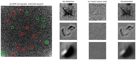
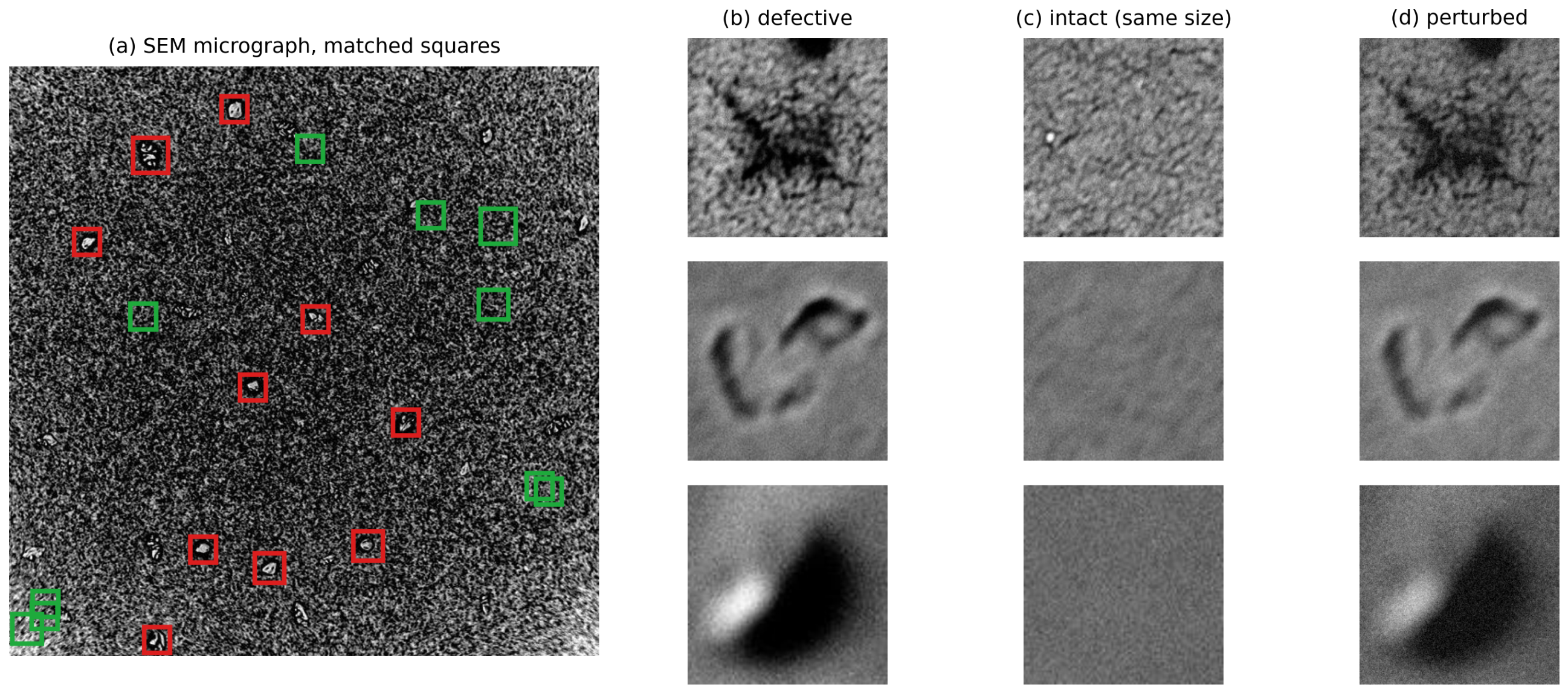
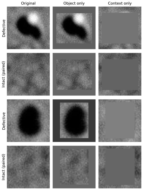
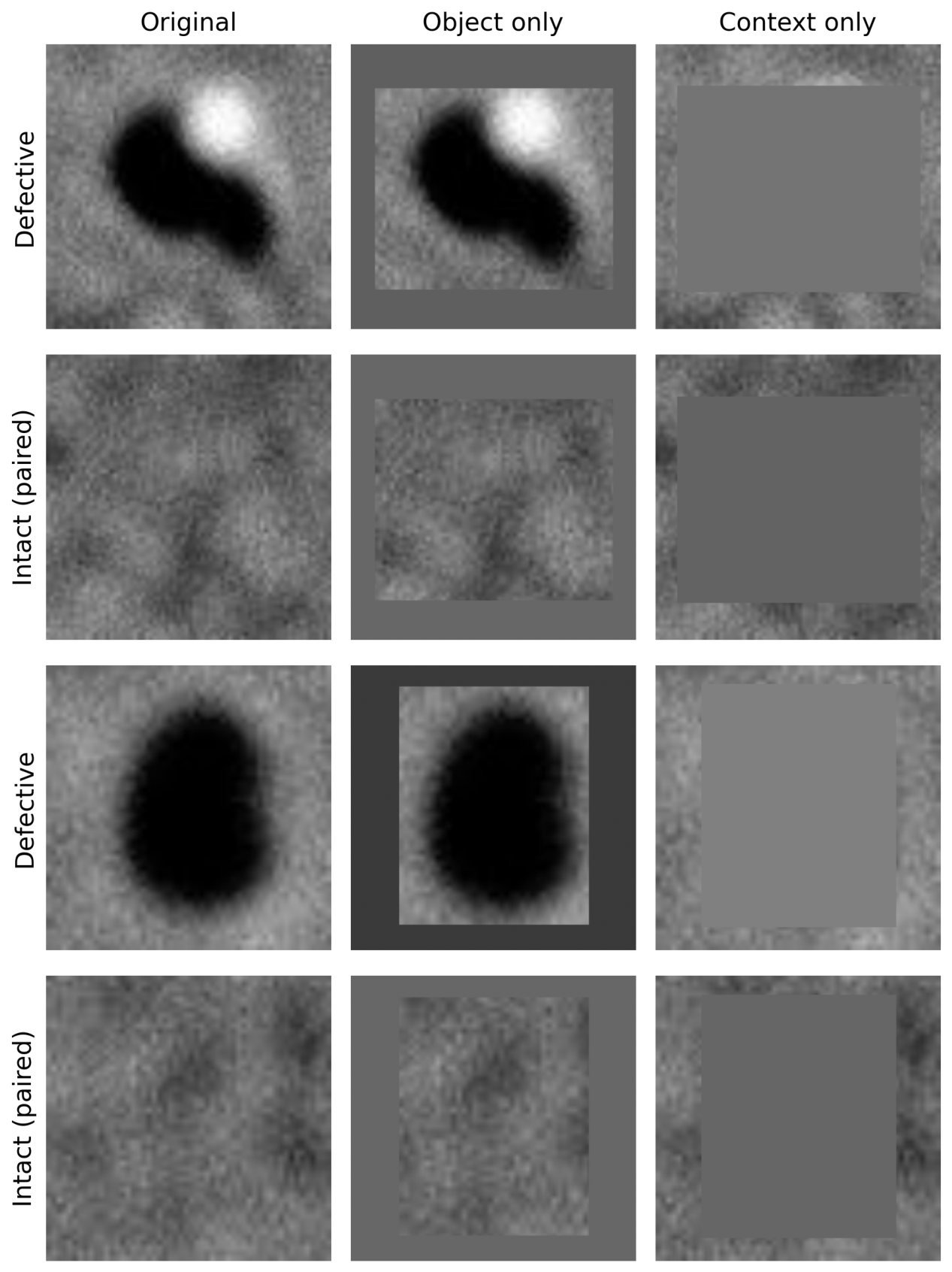
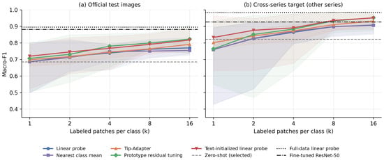
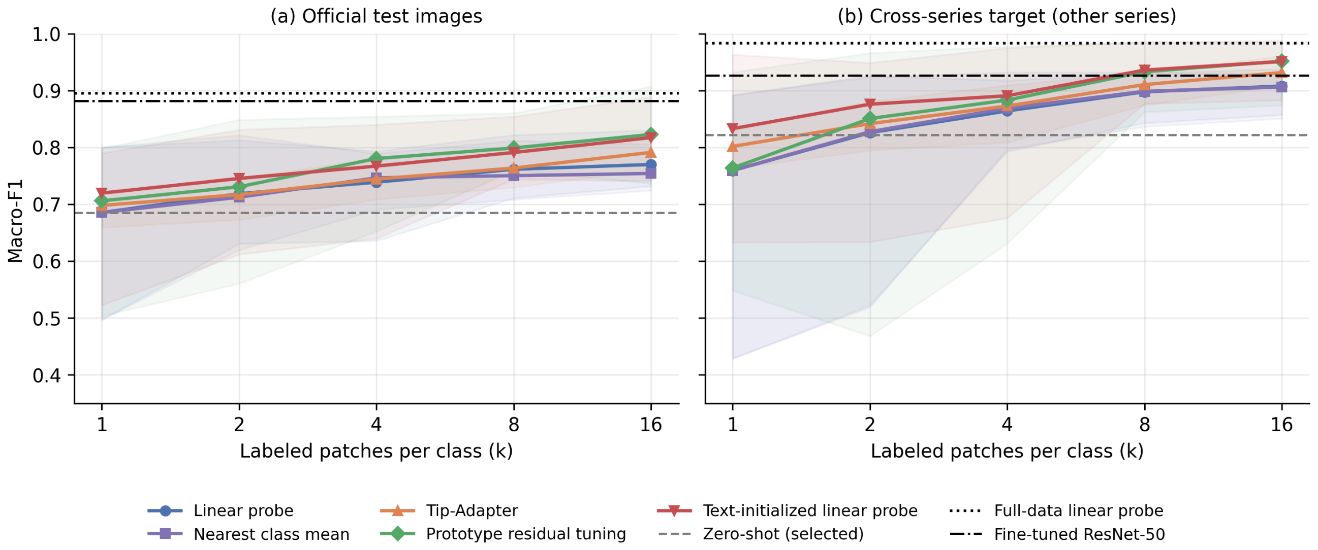
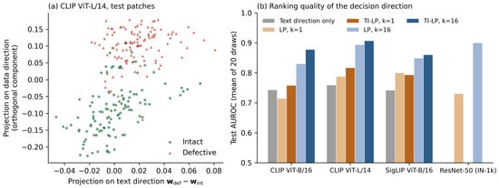
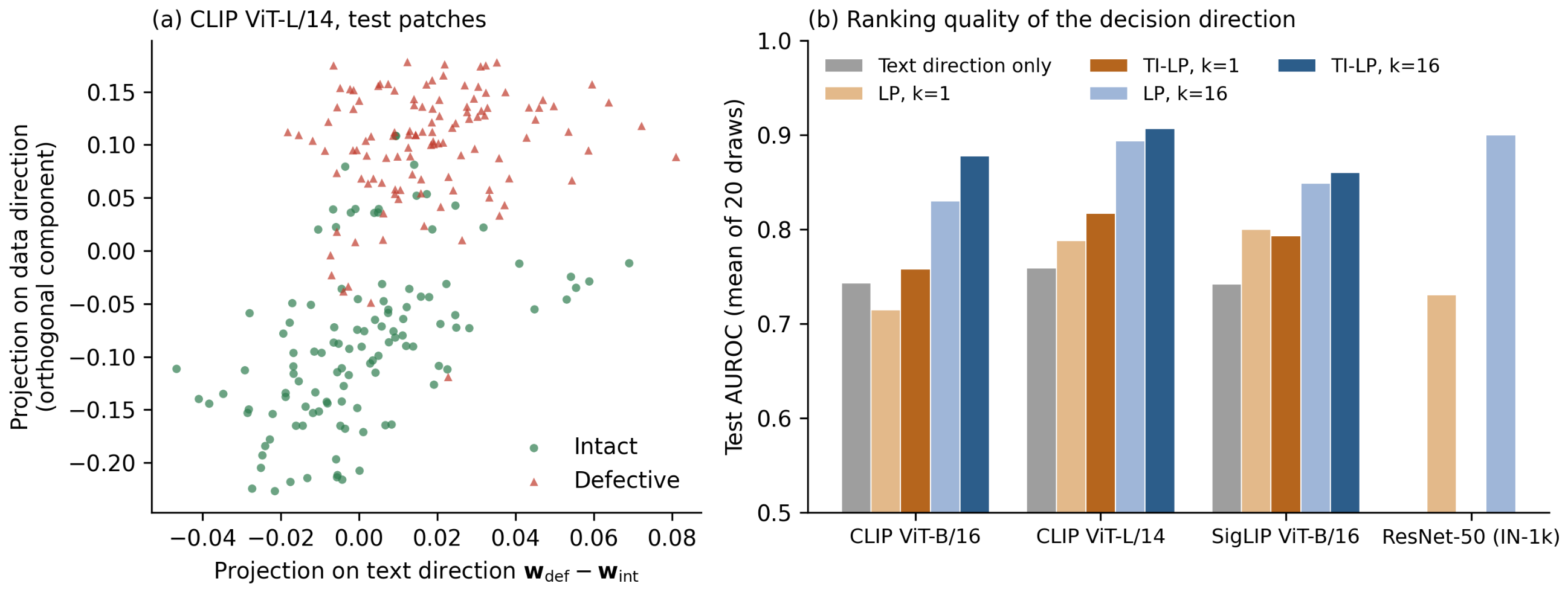
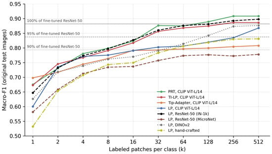
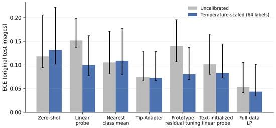
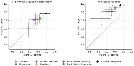
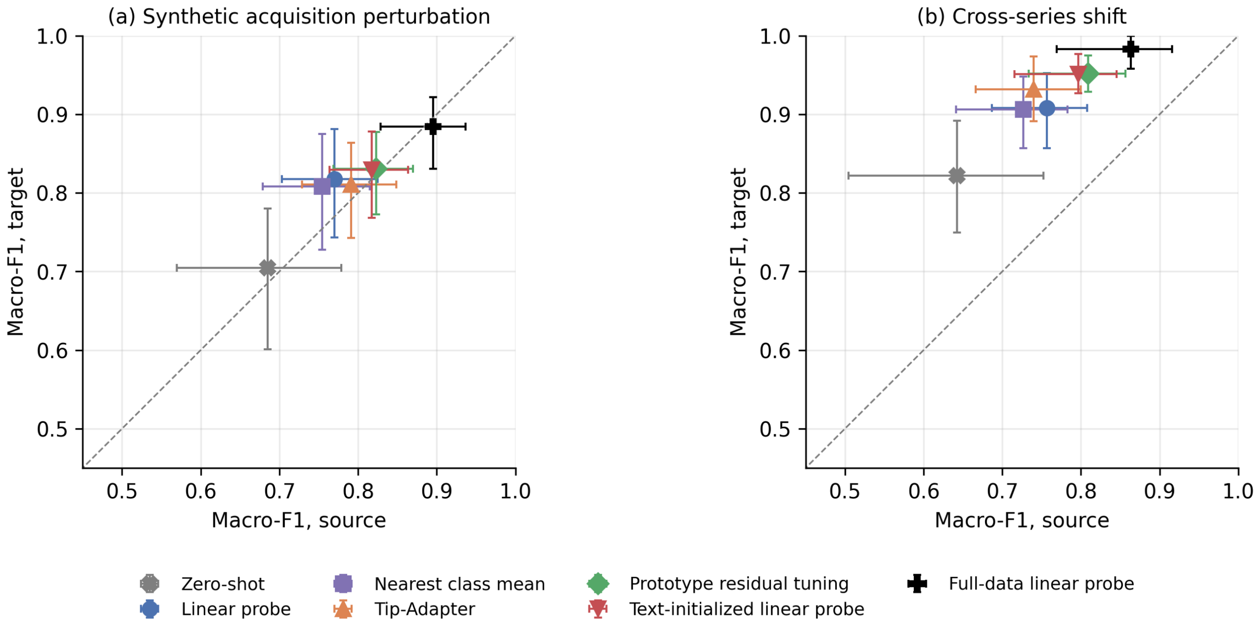

Disclaimer/Publisher’s Note: The statements, opinions and data contained in all publications are solely those of the individual author(s) and contributor(s) and not of MDPI and/or the editor(s). MDPI and/or the editor(s) disclaim responsibility for any injury to people or property resulting from any ideas, methods, instructions or products referred to in the content. |
© 2026 by the authors. Licensee MDPI, Basel, Switzerland. This article is an open access article distributed under the terms and conditions of the Creative Commons Attribution (CC BY) license.