


Abstract
The decline in groundwater storage (GWS) poses a critical threat to water security in semi-arid regions where increasing agricultural water demand and climate variability are increasing pressure on aquifers. This study presents a novel hybrid modeling framework integrating multi-source satellite and climate data (GRACE, GLDAS, TerraClimate, and MODIS) with machine learning and explanatory artificial intelligence techniques for the long-term assessment and interpretation of GWS anomalies in the data-poor Iğdır Basin. Three different modeling approaches were developed: XGBoost, Long Short-Term Memory (LSTM) networks, and their combined model, and interpreted using the Shapley Additive Explanations (SHAP) method. The results showed a significant long-term decreasing trend in groundwater storage anomalies at a rate of −0.87 mm per month during the 2002–2016 period, indicating continuous depletion. The LSTM model demonstrated the best performance with R2 of 0.59, RMSE of 19.5 mm, and MAE of 15.1 mm, revealing the dominant role of temporal dependencies in groundwater systems. SHAP analysis identified lagged groundwater anomalies (especially GWS_lag3) as the most effective predictors; this may reflect the memory effect and lagged response specific to semi-arid aquifer systems, but this interpretation needs to be validated in different study areas. Snow water equivalent and total water storage anomalies also emerged as significant determinants, while the direct effect of instantaneous precipitation was found to be limited. This study addresses significant gaps in the literature by combining sequence-based modeling with model interpretability in a semi-arid closed basin. The findings highlight the necessity of using system memory and explainable artificial intelligence together for reliable groundwater prediction. While the proposed hybrid approach has the potential for application in other semi-arid regions, its broader usability needs to be supported by independent validation studies under different hydrogeological and climatic conditions.
1. Introduction
Groundwater is one of the most critical freshwater resources for agricultural production, drinking water supply, and ecosystem sustainability, especially in semi-arid and arid regions. Due to the limited surface water resources in such regions, groundwater acts as an important buffer against climate variability [1,2,3]. However, in recent years, increasing population, agricultural irrigation activities, and the effects of climate change have led to serious reductions in groundwater reserves worldwide. Therefore, understanding the temporal dynamics of groundwater storage and revealing its long-term changes is of great importance for sustainable water management [4,5,6].
Satellite-based observations have made significant progress in monitoring large-scale hydrological processes in recent years. In particular, the Gravity Recovery and Climate Experiment (GRACE) satellite mission enables the identification of total water storage (TWS) anomalies and, when used in conjunction with surface models (e.g., GLDAS), allows for the indirect prediction of groundwater variation [7]. However, GRACE data cannot directly generate predictions and has limited temporal resolution. This necessitates the use of data-driven modeling approaches in the study of historical groundwater variability [8,9].
Machine learning (ML) methods stand out as powerful tools in modeling complex and nonlinear hydrological processes. Extreme Gradient Boosting (XGBoost) and Long Short-Term Memory (LSTM) models are widely used in groundwater modeling because they can work with high-dimensional datasets and capture nonlinear and temporal relationships. However, these methods cannot adequately represent the natural lagged response of groundwater systems and memory effects. In contrast, deep learning-based Long Short-Term Memory (LSTM) networks offer more successful results in learning dependencies in time series data [10,11,12].
One of the most significant limitations of advanced modeling techniques is the lack of interpretability. Shapley Additive Explanations (SHAP), an explainable artificial intelligence method, allows for the interpretation of model outputs and the determination of the relative importance of variables [13,14]. Such approaches are critical because they not only provide high accuracy but also allow for the physical interpretation of model results.
Although numerous studies in the literature have examined groundwater variations using satellite data or machine learning methods, some significant gaps stand out. First, much of the current research focuses on short-term analyses. In contrast, studies on long-term groundwater variability based on satellite observations are still limited, especially in semi-arid basins. Second, hybrid modeling frameworks that combine tree-based machine learning, deep learning, and stochastic approaches are not sufficiently developed. Third, lagged effects and system memory in groundwater systems have not yet been adequately elucidated using explainable models. Finally, regions like the Iğdır Basin in Eastern Anatolia, which have semi-arid climatic characteristics and high water stress potential, have only been studied to a limited extent in the literature.
This study proposes a hybrid modeling approach integrating multi-source satellite and climate data (GRACE, GLDAS, MODIS, and TerraClimate) to address the aforementioned gaps. The main objectives of this study are: (i) to characterize the temporal and spatial variability of groundwater storage anomalies; (ii) to develop predictive models based on XGBoost, LSTM, and ensemble learning approaches; and (iii) to quantitatively determine the relative contributions of hydrological and climatic drivers using the SHAP framework.
The innovative aspects of this study stand out in three key areas. First, different satellite and climate datasets are brought together in a single integrated modeling framework. Second, high-accuracy models (LSTM and XGBoost) are used in conjunction with the explainable SHAP method, ensuring both high performance and interpretability. Thirdly, the relative importance of known groundwater memory effects and delayed responses was quantitatively assessed using SHAP-based explainable artificial intelligence.
In these respects, this study contributes to the understanding of groundwater dynamics in semi-arid regions and offers a comprehensive and innovative approach in the field of data-driven hydrological modeling.
2. Data and Methods
2.1. Study Area
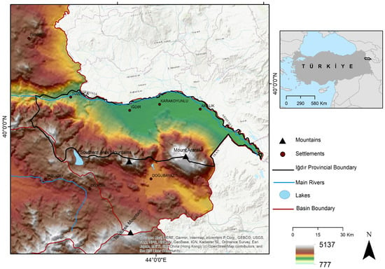
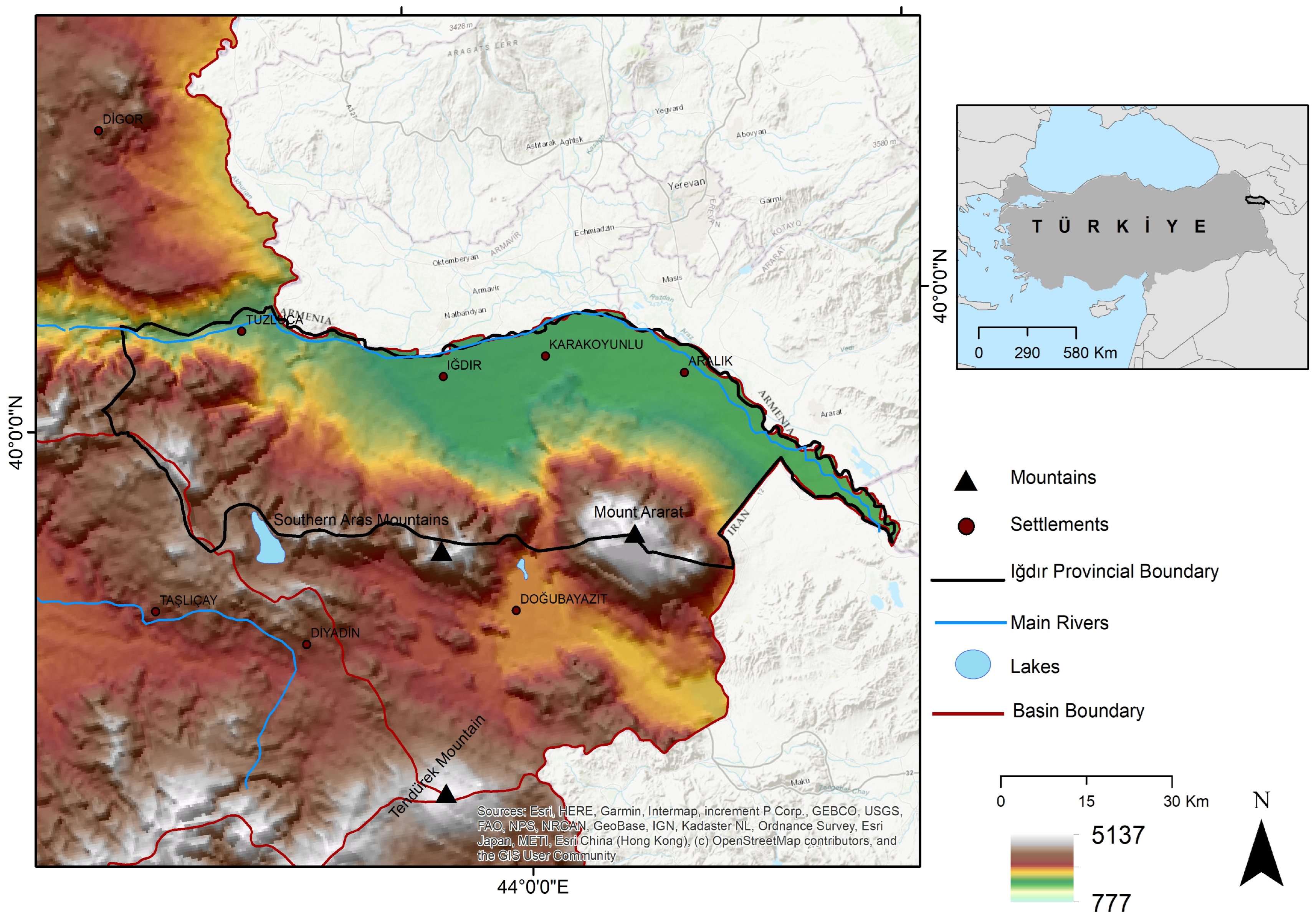
The study area, located in Iğdır province, is a typical closed basin reflecting the semi-arid climatic characteristics of Eastern Anatolia and is one of the regions with the lowest rainfall in Türkiye. The region has a hydroclimatic structure where the average annual rainfall varies between approximately 250 and 350 mm, while high evaporation and evapotranspiration values are observed. Although the Aras River and the surrounding alluvial plains are important for agricultural activities, water resources are largely dependent on groundwater. The topography consists of wide plains extending from the high mountainous areas around Mount Ağrı in the south to the north, which directly affects surface runoff and groundwater recharge. Semi-arid climatic conditions, irregular rainfall regimes, and increasing agricultural water use increase the risk of groundwater depletion in the region and make sustainable water management critical (Figure 1).
Figure 1.
Location of the study area.
Groundwater recharge is mainly provided by rainfall infiltration, snowmelt from the surrounding high areas, seepage from the Aras River and its tributaries, and irrigation return runoff during the irrigation season. Groundwater discharge is primarily controlled by agricultural groundwater extraction, drinking and domestic water use, evapotranspiration, and natural groundwater flow into surface drainage systems. In recent years, increased groundwater use due to intensive agricultural activities has made groundwater the primary source of freshwater for irrigation and drinking water supply in the basin. Therefore, sustainable management of groundwater resources under semi-arid climatic conditions has become increasingly critical for the region.
2.2. Data
GRACE is a satellite mission developed by NASA and DLR and launched in 2002. It monitors changes in global water storage by measuring variations in the Earth’s gravitational field. Using a twin satellite system, GRACE detects small variations in the gravitational field [15]. Although it does not directly measure groundwater, it allows for the indirect calculation of groundwater changes by identifying total water storage (TWS) anomalies. This data is often used in conjunction with land surface models such as GLDAS to obtain groundwater storage anomalies. With a temporal resolution of one month and a spatial resolution of approximately 300 km (Table 1), GRACE data is critical for large-scale hydrological analyses and drought studies and is currently being continued by the GRACE-FO mission [16]. Land surface water storage anomalies (TWSA) derived from GRACE were used to characterize groundwater storage changes in the Iğdır Closed Basin. Given the relatively coarse spatial resolution (~300 km) of GRACE observations and the small size of the study area, spatial scale limitations and potential signal leakage effects were addressed through leakage correction procedures. The corrected GRACE signals were then downscaled using high-resolution hydroclimatic and remote sensing variables to improve their spatial representation at the basin scale. These preprocessing steps minimized the impact of signals originating from surrounding areas and enabled a more accurate assessment of groundwater storage variability in the Iğdır Closed Basin.
Table 1.
Datasets used in the study and their main characteristics.
In this study, the GLDAS Noah land surface model (GLDAS_NOAH025_M_2.1) was used to obtain soil moisture and snow water equivalent (SWE) data. The Noah model was preferred because it provides long-term and consistent monthly data records and is widely used in many hydrological and groundwater studies.
GLDAS is a data assimilation system developed by NASA that combines meteorological observations with satellite data to simulate land surface processes [17,18]. By providing basic hydrological variables such as soil moisture, snow water equivalent (SWE), surface runoff, and evapotranspiration at regular time intervals, it enables the analysis of components of the water cycle [19,20]. Widely used in conjunction with GRACE data, GLDAS plays a critical role in separating the groundwater component from total water storage. With various model options such as Noah, VIC, and CLSM, and its high temporal resolution (3-h, daily, and monthly), GLDAS is a reliable dataset widely used in hydrological modeling, drought analysis, and water resource management studies [21,22].
TerraClimate is a dataset widely used for hydroclimatic analyses on a global scale, providing monthly climate data with high spatial resolution (~4 km). This dataset combines observational climate data with reanalysis products to provide long-term and consistent representations of precipitation, temperature, potential evapotranspiration (PET), soil moisture, and water budget components [23,24]. Particularly suitable for water budget analyses and drought studies, TerraClimate plays an important role in modeling groundwater changes by accurately representing the spatial and temporal variation of hydrological processes when used in conjunction with datasets such as GRACE and GLDAS [25].
2.3. Methods
The TWS anomaly is an indicator derived from GRACE satellite data that represents the deviation of total water storage in a region from its long-term average. TWS represents the sum of groundwater, soil moisture, snow water equivalent, and surface water components, and the anomaly value is calculated as the difference between the total amount of water in a specific time period and the reference average. Positive TWS anomalies indicate water accumulation (wet periods), while negative anomalies indicate water loss (dry periods). In this study, TWS anomalies were used as baseline data to determine changes in groundwater storage, and groundwater anomalies were obtained by evaluating them together with GLDAS data [26,27].
The groundwater storage anomaly (GWSA) was calculated using the TWSA obtained from GRACE satellite data, and the soil moisture anomaly (SMSA) and snow water equivalent anomaly (SWEA) obtained from the GLDAS dataset. In this study, the widely accepted water budget approach was adopted, and the groundwater storage anomaly was obtained using the following Equation (1):
GWSA = TWSA − SMSA − SWEA
Here, the groundwater storage anomalies (GWSA, mm) were calculated as the residual component of total terrestrial water storage anomalies (TWSA, mm) derived from GRACE observations after accounting for soil moisture storage anomalies (SMSA, mm) and snow water equivalent anomalies (SWEA, mm) obtained from the GLDAS dataset.
All variables used in the study were evaluated on a monthly time scale and converted into anomaly values based on the average of the study period. These values were then spatially centered within the boundaries of the Iğdır Basin and used as input variables for machine learning models. Due to the limited surface water storage in the study area and the negligible level of plant water storage under semi-arid climatic conditions, these components were not included in the GWSA calculation.
Soil Moisture Anomaly (SMSA) is a hydrological indicator representing the deviation of measured soil moisture values from the long-term average over a specific time period. This anomaly is usually calculated using soil moisture data obtained from land surface models such as GLDAS and reveals changes in soil moisture, a significant component of the water cycle. Positive soil moisture anomalies represent wetter than normal conditions, while negative anomalies represent drought or water scarcity. In groundwater analysis, soil moisture anomalies play a critical role in the separation of groundwater components within total water storage and contribute to more accurate calculation of groundwater storage anomalies, especially when used in conjunction with GRACE data [28,29].
TerraClimate anomaly variables are indicators derived from the TerraClimate dataset that represent the deviation of each hydroclimatic variable from its long-term average. Specifically, the precipitation anomaly represents the difference between precipitation in a given period and the long-term normal; the soil moisture anomaly represents the change in the amount of water held in the soil; the temperature anomaly represents the deviation from the average temperature; the surface runoff anomaly represents changes in surface runoff; and the PET anomaly represents differences in atmospheric water demand. These anomaly variables are critical in analyzing changes in drought, water surplus, and energy balance in hydrological systems and are widely used in modeling changes in groundwater storage, particularly in identifying lagged effects and climatic stressors [30,31].
To represent the temporal continuity and memory properties of groundwater storage anomalies, lagged groundwater storage anomaly variables (GWS_lag1–GWS_lag6) were included in the model. Responses in groundwater systems often occur with delays due to recharge processes, groundwater flow dynamics, and seasonal hydroclimatic variability. In this study, GWS_lag1–GWS_lag6 variables were created using 1 to 6 months lagged values of the groundwater storage anomaly time series, respectively. Thus, each lagged variable represents the impact of groundwater conditions in previous months on available groundwater storage. The six-month lag window was chosen because it provides a sufficient time period to capture short- and medium-term memory effects commonly observed in groundwater systems. This choice does not represent the physical flow time for a particular aquifer; instead, it allows machine learning models to identify the most meaningful temporal dependencies within the existing data set. Additionally, since the study data set consists of only 177 monthly observations, using longer lag windows was not preferred as it would reduce the sample size and increase the model complexity, thus increasing the risk of overfitting.
The selected 1–6 month delay window was not chosen to represent the physical groundwater flow or transport time of the aquifer. Instead, it was adopted as a practical modeling strategy to capture short- and medium-term memory effects commonly observed in groundwater systems while maintaining a sufficient number of training samples. Since the dataset consists of only 177 months of observations, testing longer delay windows would reduce the effective sample size and increase model complexity, raising the risk of overfitting. Future studies are recommended to evaluate alternative delay structures using sensitivity analyses and hydrogeological observations to determine the optimal response time for the aquifer system.
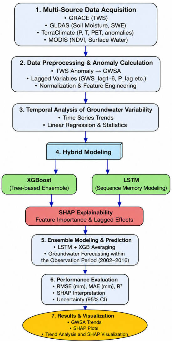
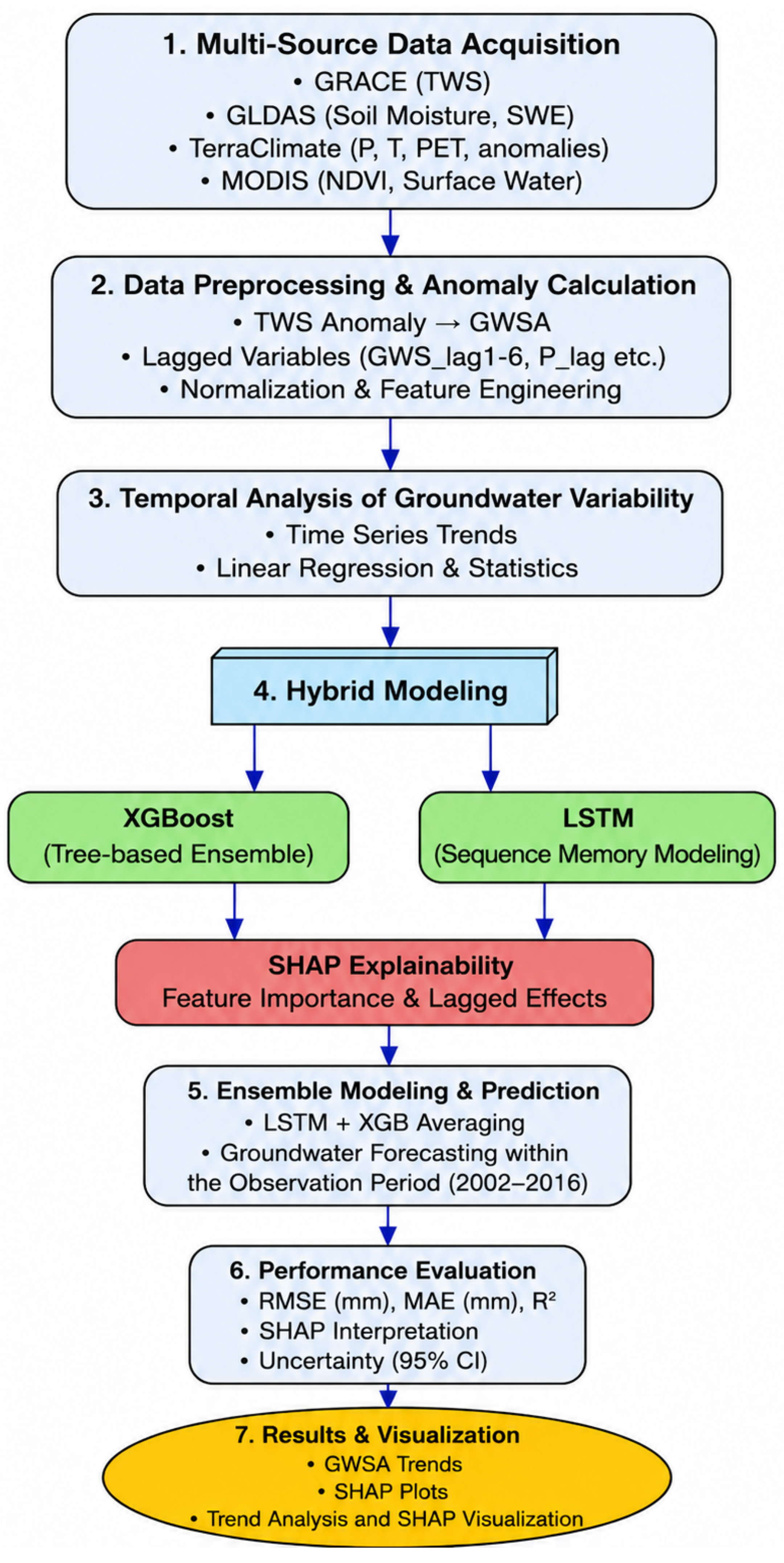
Machine learning refers to data-driven modeling approaches that can predict and classify by learning patterns in large and complex datasets. Machine learning methods offer significant advantages in the analysis of nonlinear and multivariate processes such as hydrological systems. In this study, tree-based algorithms, particularly XGBoost, were used to model groundwater storage changes (Figure 2). These methods stand out because they can capture complex relationships between variables and work effectively with high-dimensional data. In addition, a deep learning-based LSTM model has been applied to better represent the temporal dependencies of groundwater systems. Thanks to the machine learning approach, groundwater changes have been predicted with high accuracy using satellite and climate data, and system dynamics have been analyzed more comprehensively [11,32].
Figure 2.
Workflow illustrating the data processing, modeling, and interpretation framework.
Prior to the model development process, all predictor variables were synchronized to monthly temporal resolution and combined into a single time-series dataset. The machine learning workflow was executed in accordance with the chronological order of the data to preserve the temporal structure of groundwater dynamics and avoid disrupting the sequential dependence between observations. The model development process included data preprocessing, creation of the GWS_lag1–GWS_lag6 lagged groundwater storage anomaly variables, model training, performance evaluation, and interpretation of model results using the SHAP method. The hyperparameters of the machine learning models were iteratively optimized throughout the model development process to improve prediction performance and reduce the risk of overfitting. The LSTM model was used to capture temporal dependencies and memory effects in groundwater storage anomalies, while the XGBoost model was used to model the nonlinear relationships between hydroclimatic variables and groundwater storage. Finally, the outputs of the individual machine learning models were compared, and the robustness of the predictions and overall model stability were improved using an ensemble model created by combining the predictions.
XGBoost (Extreme Gradient Boosting) is an advanced machine learning algorithm based on the gradient boosting approach and distinguished by its high-performance prediction capabilities. XGBoost aims to minimize previous errors in each new model by sequentially training decision trees, which are weak learners, thus creating a robust ensemble model. Features such as regularization, early stopping, and parallel processing allow it to reduce overlearning while ensuring high accuracy. XGBoost is particularly successful in modeling nonlinear relationships and producing fast and effective results on large datasets. In this study, the XGBoost model was used to predict groundwater storage anomalies and contributed to revealing the complex relationships between hydrological and climatic variables [33,34,35,36].
3. Results
3.1. Spatiotemporal Analysis of Groundwater Storage Anomalies
Groundwater storage anomaly (GWSA) showed significant temporal variability, ranging from approximately −180 to +173 mm, indicating pronounced fluctuations between dry and wet periods. The near-zero mean value confirms that the anomaly dataset has been appropriately normalized. The relatively high standard deviation (~77 mm) indicates significant interannual variability in groundwater storage, likely stemming from climatic variability and hydrological processes in the study area.
Table 2 summarizes the distribution of the dataset of 177 observations. As expected from the anomaly normalization procedure, the mean value is close to zero, as anomalies are calculated as deviations from the reference mean. However, the high standard deviation of 77.4 mm indicates significant variability between observations. The wide range between the minimum (−180.8 mm) and maximum (173.2 mm) values also supports this high distribution. Analysis of the quartiles reveals that the lower quartile (Q1) is −53.7 mm and the upper quartile (Q3) is 60.9 mm, indicating that most of the data clusters within this range. The median value of 3.5 mm suggests that the distribution is centered around zero. While the proximity of the mean and median suggests a generally symmetrical distribution, the magnitude of the minimum and maximum values may indicate the presence of outliers. Overall, the dataset exhibits a structure that is centered around zero but has a wide distribution.
Table 2.
GWS Anomaly Statistics.
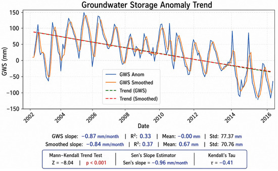
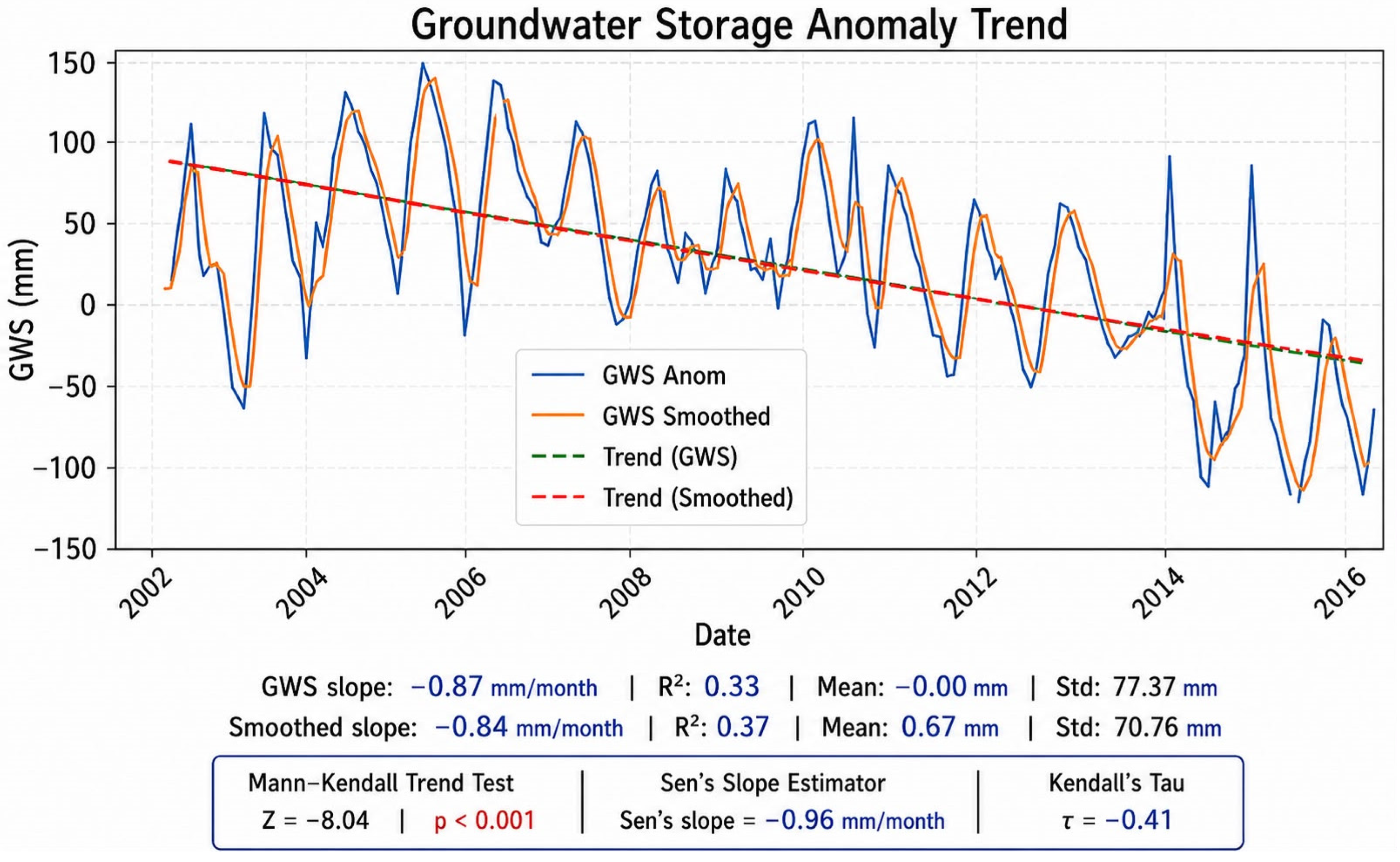
The GWSA time series exhibits strong temporal variability, with significant seasonal oscillations and an overall decreasing trend throughout the study period (2002–2016). Deviation values range from approximately −180 mm to +170 mm, indicating significant differences between wet and dry periods. Although the series shows considerable variability, the long-term linear trend points to a steady decrease in groundwater storage. Linear trend analysis shows that the slope of the original GWS anomaly is negative (−0.87 mm/time step) and the slope of the corrected series is also negative (−0.84 mm/time step), confirming a sustained decrease in groundwater storage over time. The coefficients of determination (R2) of the original and corrected series are 0.33 and 0.37, respectively, indicating a moderate but significant trend. The corrected series reduces short-term variations, making the underlying trend clearer (Figure 3). The near-zero mean of the anomaly series indicates appropriate normalization, while the relatively high standard deviation (77.4 mm for the original series and 70.8 mm for the corrected series) reflects high interannual variability. This variability can be attributed to climatic factors such as changes in precipitation, evapotranspiration, and drought, which have significant effects on groundwater recharge and depletion.
Figure 3.
Temporal variation and linear trend of groundwater storage anomaly (GWSA, mm) for the period 2002–2016. All groundwater storage values are expressed in millimeters (mm).
The slope of approximately −0.87 mm/month determined in the linear regression analysis corresponds to an annual groundwater storage loss of approximately −10.5 mm/year. This result indicates a continuous decrease in groundwater reserves in the Iğdır Basin throughout the study period. In a basin where groundwater is heavily used, particularly for agricultural irrigation, this decreasing trend poses significant risks for future irrigation water supply, water security during drought periods, and the sustainable management of groundwater resources. Therefore, regular monitoring of groundwater extraction, improvement of water use efficiency, and evaluation of sustainable management strategies such as artificial recharge are of great importance.
3.2. SHAP
SHAP analysis was applied only to the XGBoost model, and the significance and contributions of the variables were interpreted. SHAP was not applied to LSTM or ensemble models because sequential deep learning models require more computationally intensive and indirect explanation methods such as KernelSHAP.
The XGBoost model, interpreted using the SHAP method, showed a prediction performance of R2 = 0.43, which is lower than the performance of the LSTM model (R2 = 0.59) using an ordered data structure. Although XGBoost provided lower prediction accuracy, the SHAP analysis offered valuable information for determining the relative importance of hydrological and climatic variables controlling groundwater storage variability. This difference is expected, as SHAP analysis is typically applied to tree-based models that may not fully capture temporal dependencies inherent in groundwater systems. Despite its lower predictive accuracy, the SHAP framework provides robust insights into feature importance, allowing the identification of key drivers controlling groundwater storage loss. Therefore, the SHAP results are primarily interpreted in terms of relative influence rather than absolute predictive performance.
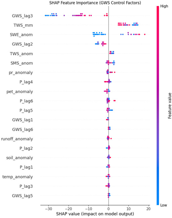
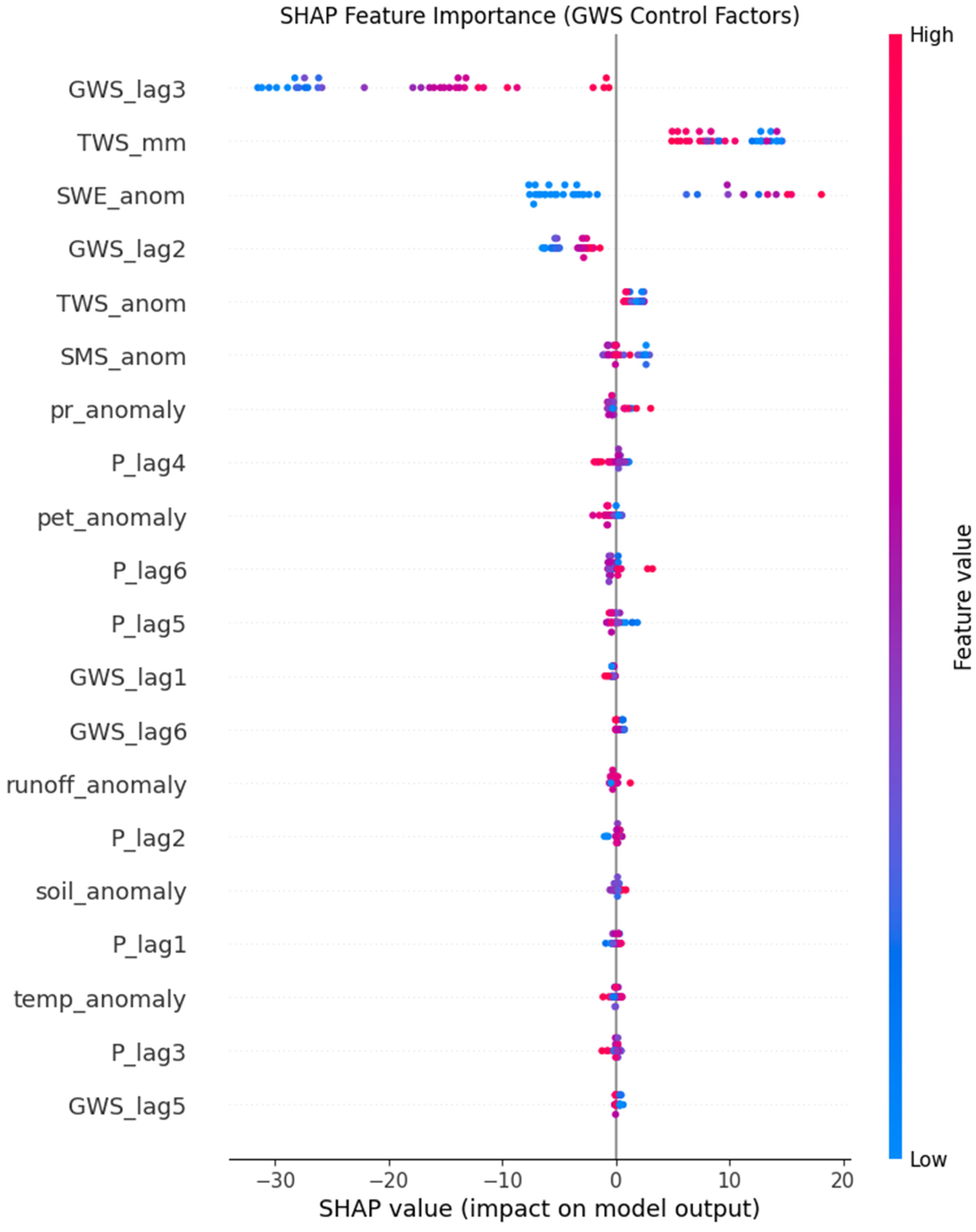
The SHAP analysis reveals that groundwater storage loss is predominantly controlled by lagged system dynamics, with the most influential variable being the three-month lagged groundwater anomaly (GWS_lag3). This variable exhibits the highest SHAP contribution, ranging approximately from −30 to +15, indicating a strong bidirectional influence on the model output. This finding provides quantitative support for previously reported groundwater memory effects within the proposed modeling framework, where current storage changes are largely governed by antecedent conditions. Such behavior is characteristic of groundwater systems, which typically respond slowly to external forcing, reflecting delayed recharge processes rather than instantaneous reactions. In addition to lagged groundwater dynamics, total water storage (TWS_mm) emerges as a key controlling factor. Higher TWS values are associated with positive SHAP contributions, indicating that integrated water storage is an important predictor of groundwater storage variations within the proposed modeling framework. This underscores the importance of considering basin-scale water availability when evaluating groundwater variability. Snow water equivalent anomalies (SWE_anom) also exhibit a significant contribution, indicating that cryospheric processes play a critical role in groundwater dynamics. The influence of SWE suggests that snowmelt contributes to delayed recharge, reinforcing the importance of seasonal storage components in sustaining groundwater systems. This represents a particularly strong finding, as it highlights the indirect but essential role of snow processes in groundwater variability. Furthermore, multiple lagged variables, including GWS_lag2 and precipitation lags (P_lag4, P_lag5, and P_lag6), demonstrate that the system exhibits a multi-month lag response. This indicates that groundwater storage loss is not governed by instantaneous climatic inputs but rather by temporally accumulated and delayed effects, reflecting the complex and buffered nature of subsurface hydrological processes. Interestingly, precipitation anomaly (pr_anomaly) shows a relatively weak direct influence on groundwater storage loss. This suggests that precipitation impacts groundwater primarily through delayed and filtered pathways rather than immediate recharge. Such a pattern is consistent with the understanding that infiltration, percolation, and subsurface flow processes introduce temporal lags between rainfall events and groundwater response. Finally, temperature and PET anomalies exhibit comparatively lower contributions, although their effects remain detectable. These variables likely act as secondary controls, influencing groundwater indirectly through evapotranspiration and soil moisture dynamics rather than serving as primary drivers. Overall, the SHAP results indicate that groundwater storage loss is governed by a combination of memory-driven processes, integrated water storage, and delayed climatic influences, with cryospheric contributions playing a non-negligible role in the system dynamics (Figure 4).
Figure 4.
SHAP-based feature importance for groundwater storage loss prediction. Red colors indicate higher feature values, whereas blue colors indicate lower feature values. SHAP values represent the contribution of each predictor to the model output.
The relatively low contribution of MODIS-based variables in the SHAP analysis indicates that vegetation status (NDVI) and surface water area have only an indirect effect on groundwater storage anomalies. While these variables primarily reflect vegetation dynamics, evapotranspiration, and surface hydrological conditions, groundwater storage in the Iğdır Basin is predominantly controlled by previous groundwater conditions, terrestrial water storage, soil moisture, and snowmelt processes. Therefore, although MODIS-based variables provide complementary environmental information, they contribute less to the prediction of groundwater storage compared to variables directly related to subsurface hydrological processes. While these variables reflect vegetation status, surface energy balance, and evapotranspiration processes, changes in groundwater storage are primarily governed by the combined effects of precipitation, soil moisture, snowmelt, and antecedent groundwater conditions. Furthermore, due to the semi-arid climate of the Iğdır Basin and intensive agricultural water use, groundwater dynamics are largely controlled by lagged hydrological processes and human-induced water withdrawals. Therefore, although MODIS variables provide complementary environmental information to the model, they showed lower relative significance values in the SHAP analysis.
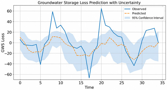
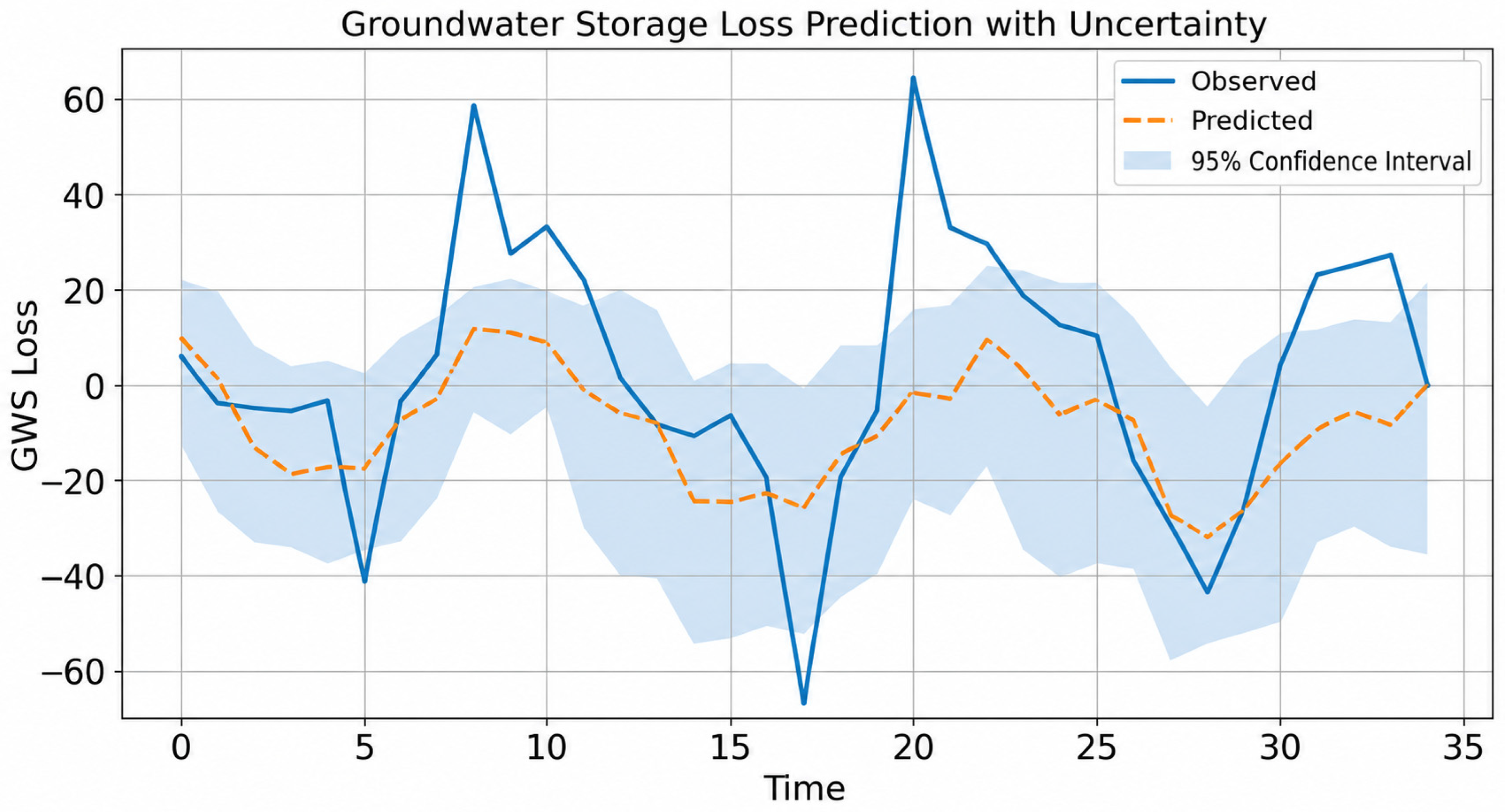
Figure 5 shows the observed, predicted, and 95% confidence intervals together. When the model outputs are examined, it is seen that the predicted series (dashed orange line) partially captures the general trend in groundwater loss. However, it is noteworthy that the model underestimates amplitude values and, in particular, does not adequately represent extreme values. This indicates that the model’s performance is limited in periods of high variance. In particular, extreme events occurring at specific time steps are not adequately captured by the model. For example, the significant negative peak (~−65) around t ≈ 17 and the strong positive peak (~+65) around t ≈ 20 are significantly underrepresented in the model predictions. This finding reveals that the model does not adequately reflect extreme hydrological processes such as extreme drought or sudden recharge. This is a weakness frequently highlighted in the literature and is a critical point that should be mentioned in published studies. In addition, the model outputs appear to exhibit a smoother structure compared to observations. While observed data exhibit more volatile and high-frequency variations, model predictions tend to dampen these variations. This indicates that the model underestimates variance and suppresses high-frequency signals, exhibiting a “damping effect.” Conversely, the model’s representation of uncertainty is quite successful. The 95% confidence interval covers observations at most points and widens, particularly during periods when extreme events occur. This shows that the model accurately reflects uncertainty even in time periods with low confidence, providing a significant advantage in terms of model reliability. Furthermore, the model appears to capture observed variations with a delay in some periods. This indicates that predictions respond to actual changes with a time lag in certain time intervals. However, this delayed response is consistent with the natural dynamics of groundwater systems and reflects the lagged behavior characteristic of the system.
Figure 5.
Time series of observed GWSA, LSTM-XGB ensemble predictions, and 95% confidence intervals (Iğdır Basin, 2002–2016).
3.3. LSTM and XGB Ensemble
The models demonstrated strong performance in reproducing moderate groundwater storage fluctuations as well as the overall long-term negative trend observed in the study period. However, extreme hydrological events were partially underestimated, particularly during periods characterized by abrupt variability.
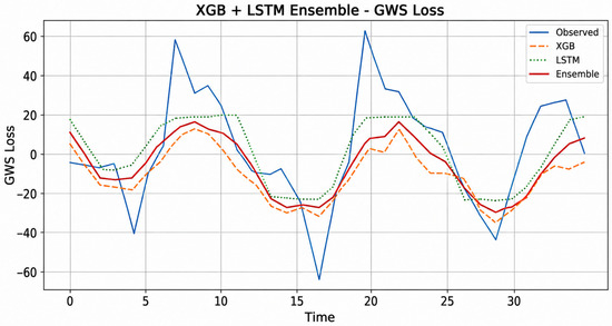
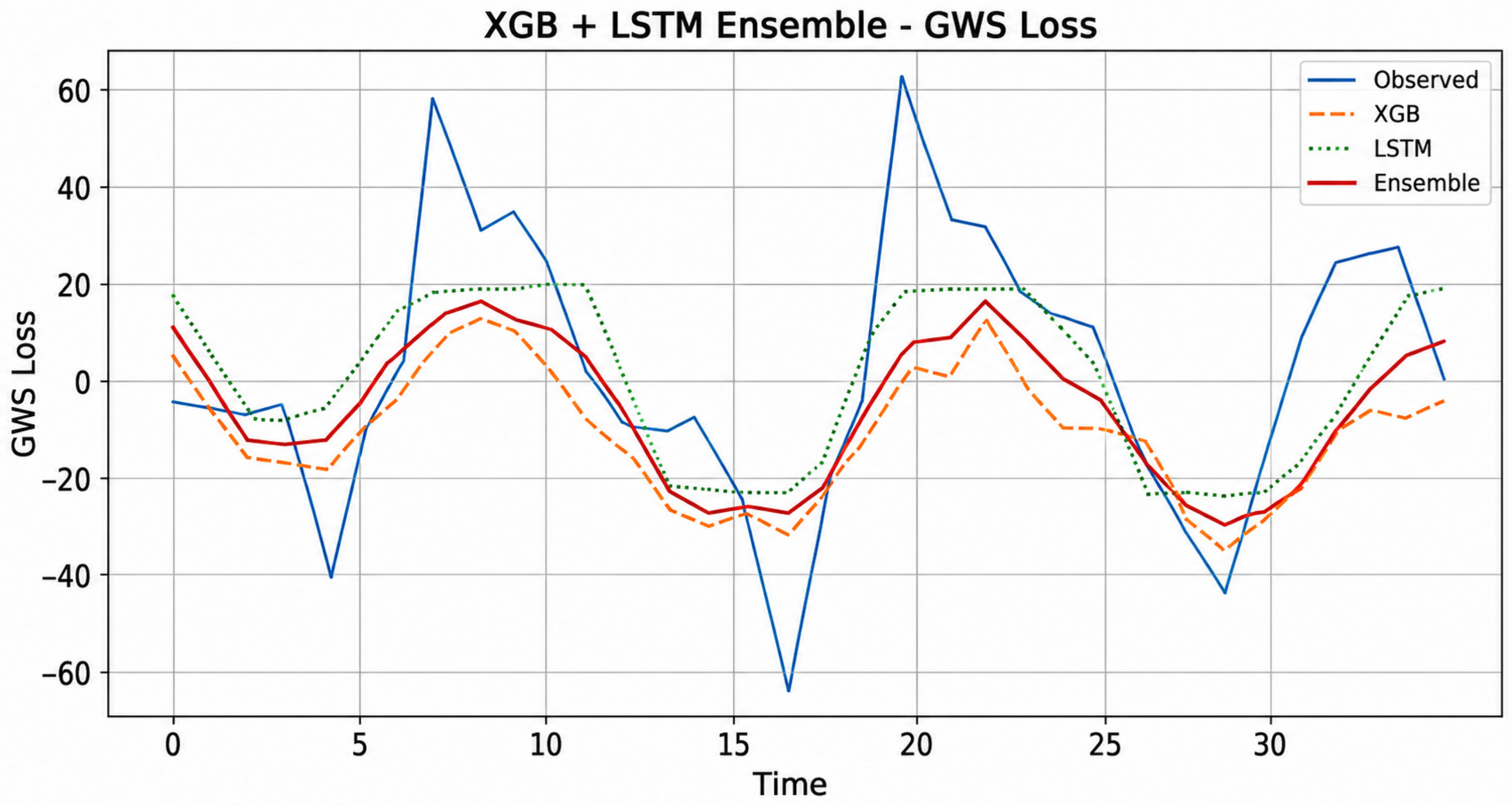
Among the tested approaches, the ensemble model provided the most balanced performance by reducing the individual limitations of the XGBoost and LSTM models. While XGBoost tended to produce slightly more volatile predictions, the LSTM model generated smoother outputs but occasionally lagged during rapid temporal transitions. In contrast, the ensemble approach effectively combined the strengths of both models. During the later stages of the time series (after time step 25), the ensemble model successfully captured both the recovery phase and the subsequent decline, indicating satisfactory generalization capability and temporal consistency (Figure 6).
Figure 6.
Time Series Comparison of Groundwater Storage Anomaly (GWS Loss) with the XGB + LSTM and Ensemble Model.
The performance comparison of the models is presented in Table 3. The LSTM model achieved the best overall performance with the lowest RMSE (19.5 mm) and MAE (15.1 mm), and the highest coefficient of determination (R2 = 0.59). These results indicate that the LSTM approach effectively captures the temporal dependencies and memory effects inherent in groundwater storage dynamics, resulting in good predictive performance. Although the ensemble model (simple averaging of XGB and LSTM) produced competitive results (R2 = 0.57), it performed slightly worse than the standalone LSTM model. This is mainly due to the relatively lower accuracy of the XGBoost model (R2 = 0.43), which introduced some noise into the ensemble prediction. XGBoost still provided acceptable performance but was outperformed by the deep learning model, as expected in a system dominated by sequential patterns. Overall, these findings confirm that for groundwater storage anomaly prediction in semi-arid regions like the Iğdır Basin, sequence-based models such as LSTM are more suitable than tree-based ensemble methods. The strong performance of LSTM (R2 ≈ 0.59) highlights the critical role of lagged effects and long-term memory in groundwater systems.
Table 3.
Comparison of model performances (RMSE, MAE, R2) for groundwater storage anomaly prediction.
4. Discussion
The negative trend identified in the Iğdır Basin is consistent with GRACE-based studies and supports the globally reported groundwater depletion trends [37]. Furthermore, previous studies have reported high agreement between GRACE observations and ground-based groundwater measurements in different regions [38], which reinforces the reliability of the multi-source datasets employed in this study.
SHAP analysis revealed the dominant influence of lagged variables, highlighting a pronounced memory effect within groundwater systems. This finding aligns with previous research indicating that hydrological systems typically exhibit delayed responses to climatic and anthropogenic drivers. Literature further confirms that groundwater storage losses are strongly linked to drought conditions and excessive extraction, with depletion rates accelerating notably during drought periods [39]. Permanent storage losses can also occur through land subsidence processes [40,41].
The LSTM model outperformed the other approaches, although its R2 value (0.589) represents only a moderate level of prediction accuracy, highlighting the importance of temporal dependencies in groundwater dynamics. In contrast, XGBoost models displayed comparatively limited predictive capability. The integration of the SHAP explainable AI method substantially enhanced the interpretability of these results. The superior performance of the LSTM model compared to the XGBoost model can be attributed to its ability to capture temporal dependencies and lagged responses that characterize groundwater systems. Unlike tree-based algorithms, LSTM explicitly learns sequential patterns and preserves information from previous time steps. This feature makes LSTM more suitable for modeling groundwater storage anomalies that gradually change over time. Similarly, the dominant importance of lagged groundwater variables determined by SHAP analysis shows that groundwater conditions from previous periods provide stronger predictive information compared to instantaneous hydroclimatic variables. This finding is consistent with the hydrogeological characteristics of the Iğdır Basin, where groundwater is stored in highly permeable alluvial units and gradually responds to recharge from precipitation, snowmelt, river seepage, and irrigation return runoff. Therefore, groundwater storage anomalies reflect the cumulative effects of previous hydrological conditions rather than instantaneous climatic stresses.
These outcomes are consistent with broader literature confirming the effectiveness of machine learning techniques in groundwater modeling [42].
It should be noted that SHAP analysis quantitatively reveals the relative contribution of predictor variables to model predictions, but does not prove physical causality. Therefore, the high significance of lagged groundwater variables should be interpreted not as direct evidence of groundwater memory processes, but as an indication that these variables have high predictive power in terms of model predictions.
Nevertheless, the models exhibited limitations in accurately capturing extreme events, a common challenge reported in hydrological modeling studies [43]. In conclusion, this study contributes to the existing body of knowledge through its integration of multi-source data (GRACE, GLDAS, TerraClimate, and MODIS) and hybrid modeling framework. The findings emphasize that accurate modeling of groundwater systems in semi-arid regions requires simultaneous consideration of temporal dependencies and explainable artificial intelligence approaches.
GWS is critically important for water security, particularly in arid and semi-arid regions. Excessive groundwater extraction, climate change, and intensified agricultural activities are driving significant water losses worldwide [44]. GRACE satellite data have become a widely adopted tool for monitoring large-scale groundwater changes. Previous studies have demonstrated the value of combining GRACE observations with hydrological models and remote sensing techniques [45]. Strong correlations between long-term groundwater losses and land subsidence have been documented in the North China Plain. Similarly, a substantial portion of total water storage loss in the Colorado Basin has been attributed to groundwater depletion [46].
Machine learning approaches have gained increasing prominence in groundwater modeling [47,48]. For instance, machine-learning-based downscaling of GRACE data successfully quantified groundwater losses during drought periods in the Central Valley [8]. Integration of downscaled GRACE data with the SWAT model enabled identification of depletion zones in the Indus Basin [49], while combined GRACE, observation well, and numerical modeling analyses revealed significant losses in the Ganga Basin. Remote sensing and InSAR techniques have further advanced groundwater management by investigating aquifer elastic behavior and storage capacity [50] and evaluating storage changes in large systems such as the Great Artesian Basin. Additional studies have highlighted the socio-economic consequences of depletion, including strong correlations between groundwater loss and farmer suicides in regions such as Maharashtra, India [51].
The findings are consistent with previous studies demonstrating that AI-based methods can be successfully applied in the assessment, prediction, and remediation of groundwater sensitivity [52,53]. In recent years, deep learning models such as LSTM and advanced tree-based methods like XGBoost, coupled with explainable AI techniques such as SHAP, have shown strong potential for modeling complex hydrological processes. However, while the vast majority of current studies focus on short-term analyses, research that comprehensively assesses long-term historical groundwater variability using integrated satellite observations and machine learning approaches is still relatively limited, particularly in semi-arid basins. The present study addresses this gap by examining long-term groundwater storage changes in the Iğdır Basin through the integration of GRACE, GLDAS, TerraClimate, and MODIS datasets with SHAP-interpreted XGBoost and LSTM models.
MODIS-derived indicators (NDVI and surface water area) were included in the data integration phase to characterize land surface conditions. However, the contribution of these variables to groundwater storage estimation was limited compared to GRACE and GLDAS-based hydrological variables. Therefore, they were not among the most dominant predictive variables in the SHAP analysis. Nevertheless, MODIS products provided complementary environmental information contributing to the interpretation of hydroclimatic conditions and land surface dynamics in the basin.
The relatively small dataset, consisting of only 177 months of observations, presents a significant limitation for training deep learning models like LSTM. Deep learning architectures generally yield more reliable and generalizable results when trained on larger datasets. Therefore, although the LSTM model performed better than other approaches in this study, the possibility of overfitting cannot be completely ruled out. To mitigate this risk, a careful modeling approach was adopted during the model development process, and the models were evaluated comparatively. However, the obtained prediction performance should be interpreted carefully, taking this limitation into account. In the future, using longer observation series, GRACE-FO data, and additional hydroclimatic variables will further improve the robustness and generalizability of the model.
Another limitation of the study is the time scope of the training dataset. The period 2002–2016 may not fully represent the frequency and magnitude of extreme hydrological events that occurred in Eastern Anatolia after 2016. Therefore, machine learning models were trained within a more limited range of hydroclimatic variability, which may have contributed to underestimating severe droughts and sudden flooding events. In future studies, the representation of extreme events and model robustness can be improved by using GRACE-FO observations and higher-resolution hydroclimatic datasets.
One of the significant limitations of the proposed model is the absence of variables that directly represent anthropogenic impacts, such as groundwater withdrawals for irrigation, agricultural water demand, and land-use changes. Therefore, the model primarily explains changes associated with natural hydroclimatic processes and the temporal memory effects of groundwater. Although anthropogenic activities contribute to groundwater depletion in the Iğdır Basin, these impacts are not directly represented as driving variables within the model, but only indirectly through observed groundwater responses. Therefore, the model should not be considered a calibrated system that fully explains human-induced groundwater depletion. Future studies are recommended to integrate irrigation statistics, groundwater withdrawal records, and land-use data.
Limitations and Future Directions
The hybrid modeling approach proposed in this study successfully captured long-term groundwater storage changes in the Iğdır Basin; however, several limitations should be acknowledged.
First, the relatively short observation period (177 months) and the coarse spatial resolution of GRACE data (~300 km) limit the model’s ability to represent high-frequency hydrological events, particularly extreme drought and rapid recharge periods. In addition, the absence of observation well data and the exclusion of human-induced factors such as groundwater extraction for irrigation and land-use change reduce the model’s representativeness at the local scale.
Second, since groundwater storage anomalies (GWSA) are derived by combining GRACE-based total water storage anomalies (TWSA) with GLDAS-based soil moisture and snow water equivalent components, using TWSA as a predictor variable introduces information leakage risk; part of the model’s apparent success may therefore stem from the mathematical dependence between predictor and target variables. Moreover, uncertainties inherent in the GRACE and GLDAS datasets propagate into the derived GWSA values. A formal uncertainty dispersion analysis was not conducted in this study due to the lack of consistent uncertainty estimates across all input datasets. Consequently, both the model performance metrics and the SHAP results should be interpreted with these limitations in mind. Future studies should apply formal error propagation analyses to quantify the contribution of each data source to the overall uncertainty in GWSA estimates.
Third, although SHAP analysis identified lagged groundwater variables as the most important predictors, this should not be interpreted as evidence of physical causality.
Finally, model comparisons relied solely on R2, RMSE, and MAE, without formal statistical significance testing between models. Since the method was evaluated only for the Iğdır Basin, its applicability to basins with different hydrogeological and climatic settings remains unverified. Future work should incorporate GRACE-FO data, higher-resolution remote sensing products, and observation well data; explore alternative lag structures and predictor variables; and test statistical significance across models to strengthen and generalize the proposed approach.
5. Conclusions
This study presented a comprehensive hybrid modeling framework for assessing and predicting long-term groundwater storage (GWS) dynamics in the semi-arid Iğdır Basin, Türkiye, by integrating multi-source satellite observations with advanced machine learning and explainable artificial intelligence techniques. The results revealed a significant negative trend in groundwater storage anomalies over the 2002–2016 period, confirming ongoing depletion consistent with regional water stress and global patterns in arid and semi-arid environments.
SHAP analysis provided critical interpretability, demonstrating that groundwater systems in the basin exhibit a pronounced memory effect, with three-month lagged groundwater anomalies (GWS_lag3) emerging as the dominant predictor. This finding underscores the delayed response characteristics of subsurface hydrological processes, where antecedent conditions exert stronger control than instantaneous climatic inputs. Among the models evaluated, the LSTM network achieved superior performance, highlighting the importance of capturing temporal dependencies in groundwater systems. The XGBoost model and the LSTM–XGBoost ensemble offered competitive yet slightly lower accuracy, while SHAP-enhanced interpretability substantially improved the understanding of variable contributions.
The developed approach addresses key gaps in the literature by integrating robust temporal modeling with explainable AI in a data-scarce semi-arid basin. These findings suggest that reliable long-term groundwater assessment may benefit from considering not only powerful predictive algorithms but also system memory and physical interpretability. These outcomes have direct implications for sustainable water resource management in Eastern Anatolia and similar semi-arid regions, where groundwater constitutes the primary water supply for agriculture and domestic use amid increasing climate variability and anthropogenic pressure.
This study presents an integrated and interpretable machine learning framework for evaluating groundwater storage dynamics in the Iğdır Basin, providing a data-driven approach that balances predictive performance with scientific transparency. However, future validation studies across different hydrogeological settings are needed to confirm the broader applicability and generalizability of the proposed framework. The findings emphasize the urgent need for integrated monitoring and adaptive management strategies to mitigate groundwater depletion and enhance water security in vulnerable semi-arid basins under changing climatic conditions. Future applications of this framework, particularly when extended with higher-resolution observations and climate projections, can support evidence-based policy decisions for long-term groundwater sustainability.
Author Contributions
M.A.Ç.: Conceptualization, data curation, investigation, resources, and writing—review and editing. Y.P.: Methodology, software, formal analysis, validation, visualization, writing—original draft, and writing—review and editing. A.B.: Software, data curation, visualization, investigation, and writing—review and editing. All authors have read and agreed to the published version of the manuscript.
Funding
This research received no external funding.
Institutional Review Board Statement
This study did not involve human participants, human data, human tissue, or animals. Therefore, ethics committee approval was not required.
Informed Consent Statement
Not applicable.
Data Availability Statement
The processed dataset supporting the findings of this study is available from the corresponding author upon reasonable request. The code used for data preprocessing, modeling, validation, and visualization is available from the corresponding author upon reasonable request.
Acknowledgments
During the preparation of this manuscript, the authors used AI-assisted language tools solely for language editing, grammar correction, and translation support. These tools were not used to generate scientific ideas, study design, methodology, data analysis, results, interpretations, or conclusions. The authors carefully reviewed and edited the final manuscript and take full responsibility for its content.
Conflicts of Interest
The authors declare no conflict of interest.
References
- Cuthbert, M.; Gleeson, T.; Moosdorf, N.; Befus, K.; Schneider, A.; Hartmann, J.; Lehner, B. Global patterns and dynamics of climate–groundwater interactions. Nat. Clim. Change 2019, 9, 137–141. [Google Scholar] [CrossRef] [Scilit]
- Scanlon, B.; Fakhreddine, S.; Rateb, A.; De Graaf, I.; Famiglietti, J.; Gleeson, T.; Grafton, R.; Jobbágy, E.; Kebede, S.; Kolusu, S.; et al. Global water resources and the role of groundwater in a resilient water future. Nat. Rev. Earth Environ. 2023, 4, 87–101. [Google Scholar] [CrossRef] [Scilit]
- Amanambu, A.; Obarein, O.; Mossa, J.; Li, L.; Ayeni, S.; Balogun, O.; Oyebamiji, A.; Oyebamiji, A.; Ochege, F.; Ochege, F. Groundwater system and climate change: Present status and future considerations. J. Hydrol. 2020, 589, 125163. [Google Scholar] [CrossRef] [Scilit]
- Shamsudduha, M.; Taylor, R. Groundwater storage dynamics in the world’s large aquifer systems from GRACE: Uncertainty and role of extreme precipitation. Earth Syst. Dyn. 2020, 11, 755–774. [Google Scholar] [CrossRef] [Scilit]
- Lin, M.; Biswas, A.; Bennett, E. Spatio-temporal dynamics of groundwater storage changes in the Yellow River Basin. J. Environ. Manag. 2019, 235, 84–95. [Google Scholar] [CrossRef] [Scilit] [PubMed]
- Li, B.; Rodell, M.; Sheffield, J.; Wood, E.; Sutanudjaja, E. Long-term, non-anthropogenic groundwater storage changes simulated by three global-scale hydrological models. Sci. Rep. 2019, 9, 10746. [Google Scholar] [CrossRef] [Scilit] [PubMed]
- Singh, A.; Jasrotia, A.; Taloor, A.; Kotlia, B.; Kumar, V.; Roy, S.; Ray, P.; Singh, K.; Singh, A.; Sharma, A. Estimation of quantitative measures of total water storage variation from GRACE and GLDAS-NOAH satellites using geospatial technology. Quat. Int. 2017, 444, 191–200. [Google Scholar] [CrossRef] [Scilit]
- Li, F.; Kusche, J.; Sneeuw, N.; Siebert, S.; Gerdener, H.; Wang, Z.; Chao, N.; Chen, G.; Tian, K. Forecasting Next Year’s Global Land Water Storage Using GRACE Data. Geophys. Res. Lett. 2024, 51, e2024GL109101. [Google Scholar] [CrossRef] [Scilit]
- Li, F.; Springer, A.; Kusche, J.; Gutknecht, B.; Ewerdwalbesloh, Y. Reanalysis and Forecasting of Total Water Storage and Hydrological States by Combining Machine Learning With CLM Model Simulations and GRACE Data Assimilation. Water Resour. Res. 2025, 61, e2024WR037926. [Google Scholar] [CrossRef] [Scilit]
- Baalousha, H. Machine Learning-Driven Calibration of MODFLOW Models: Comparing Random Forest and XGBoost Approaches. Geosciences 2025, 15, 303. [Google Scholar] [CrossRef] [Scilit]
- Zhang, J.; Liu, K.; Wang, M. Downscaling Groundwater Storage Data in China to a 1-km Resolution Using Machine Learning Methods. Remote Sens. 2021, 13, 523. [Google Scholar] [CrossRef] [Scilit]
- Sahour, S.; Khanbeyki, M.; Gholami, V.; Sahour, H.; Kahvazade, I.; Karimi, H. Evaluation of machine learning algorithms for groundwater quality modeling. Environ. Sci. Pollut. Res. 2023, 30, 46004–46021. [Google Scholar] [CrossRef] [Scilit] [PubMed]
- Ning, Y.; Ong, M.E.H.; Chakraborty, B.; Goldstein, B.A.; Ting, D.S.W.; Vaughan, R.; Liu, N. Shapley variable importance cloud for interpretable machine learning. Patterns 2022, 3, 100452. [Google Scholar] [CrossRef] [Scilit] [PubMed]
- Gebreyesus, Y.; Dalton, D.; De Chiara, D.; Chinnici, M.; Chinnici, A. AI for Automating Data Center Operations: Model Explainability in the Data Centre Context Using Shapley Additive Explanations (SHAP). Electronics 2024, 13, 1628. [Google Scholar] [CrossRef] [Scilit]
- Tapley, B.D.; Bettadpur, S.; Watkins, M.; Reigber, C. The gravity recovery and climate experiment: Mission overview and early results. Geophys. Res. Lett. 2004, 31, L09607. [Google Scholar] [CrossRef] [Scilit]
- Chen, J.; Cazenave, A.; Dahle, C.; Llovel, W.; Panet, I.; Pfeffer, J.; Moreira, L. Applications and challenges of GRACE and GRACE follow-on satellite gravimetry. Surv. Geophys. 2022, 43, 305–345. [Google Scholar] [CrossRef] [Scilit] [PubMed]
- Rodell, M.; Houser, P.; Jambor, U.; Gottschalck, J.; Mitchell, K.; Meng, C.; Arsenault, K.; Cosgrove, B.; Radakovich, J.; Bosilovich, M.; et al. The Global Land Data Assimilation System. Bull. Am. Meteorol. Soc. 2004, 85, 381–394. [Google Scholar] [CrossRef] [Scilit]
- Kumar, S.; Jasinski, M.; Mocko, D.; Rodell, M.; Borak, J.; Li, B.; Beaudoing, H.; Peters-Lidard, C. NCA-LDAS Land Analysis: Development and Performance of a Multisensor, Multivariate Land Data Assimilation System for the National Climate Assessment. J. Hydrometeorol. 2017, 20, 1571–1593. [Google Scholar] [CrossRef] [Scilit]
- Lv, M.; Lu, H.; Yang, K.; Xu, Z.; Lv, M.; Huang, X. Assessment of Runoff Components Simulated by GLDAS against UNH–GRDC Dataset at Global and Hemispheric Scales. Water 2018, 10, 969. [Google Scholar] [CrossRef] [Scilit]
- Wu, Z.; Feng, H.; He, H.; Zhou, J.; Zhang, Y. Evaluation of Soil Moisture Climatology and Anomaly Components Derived From ERA5-Land and GLDAS-2.1 in China. Water Resour. Manag. 2021, 35, 629–643. [Google Scholar] [CrossRef] [Scilit]
- Tangdamrongsub, N. Comparative Analysis of Global Terrestrial Water Storage Simulations: Assessing CABLE, Noah-MP, PCR-GLOBWB, and GLDAS Performances during the GRACE and GRACE-FO Era. Water 2023, 15, 2456. [Google Scholar] [CrossRef] [Scilit]
- Ali, S.; Wang, Q.; Liu, D.; Fu, Q.; Rahaman, M.; Faiz, M.; Cheema, M. Estimation of spatio-temporal groundwater storage variations in the Lower Transboundary Indus Basin using GRACE satellite. J. Hydrol. 2021, 605, 127315. [Google Scholar] [CrossRef] [Scilit]
- Abatzoglou, J.; Dobrowski, S.; Parks, S.; Hegewisch, K. TerraClimate, a high-resolution global dataset of monthly climate and climatic water balance from 1958–2015. Sci. Data 2018, 5, 170191. [Google Scholar] [CrossRef] [Scilit] [PubMed]
- Gebrechorkos, S.; Leyland, J.; Dadson, S.; Cohen, S.; Slater, L.; Wortmann, M.; Ashworth, P.; Bennett, G.; Boothroyd, R.; Cloke, H.; et al. Global-scale evaluation of precipitation datasets for hydrological modelling. Hydrol. Earth Syst. Sci. 2024, 28, 3099–3118. [Google Scholar] [CrossRef] [Scilit]
- Wiwoho, B.; Astuti, I. Runoff observation in a tropical Brantas watershed as observed from long-term globally available TerraClimate data 2001–2020. Geoenviron. Disasters 2022, 9, 12. [Google Scholar] [CrossRef] [Scilit]
- Shen, Y.; Zheng, W.; Zhu, H.; Yin, W.; Xu, A.; Pan, F.; Wang, Q.; Zhao, Y. Inverted Algorithm of Groundwater Storage Anomalies by Combining the GNSS, GRACE/GRACE-FO, and GLDAS: A Case Study in the North China Plain. Remote Sens. 2022, 14, 5683. [Google Scholar] [CrossRef] [Scilit]
- Fatolazadeh, F.; Eshagh, M.; Goïta, K.; Wang, S. A New Spatiotemporal Estimator to Downscale GRACE Gravity Models for Terrestrial and Groundwater Storage Variations Estimation. Remote Sens. 2022, 14, 5991. [Google Scholar] [CrossRef] [Scilit]
- Xiao, R.; He, X.; Zhang, Y.; Ferreira, V.; Chang, L. Monitoring Groundwater Variations from Satellite Gravimetry and Hydrological Models: A Comparison with in-situ Measurements in the Mid-Atlantic Region of the United States. Remote Sens. 2015, 7, 686–703. [Google Scholar] [CrossRef] [Scilit]
- Skaskevych, A.; Lee, J.; Jung, H.; Bolten, J.; David, J.; Policelli, F.; Goni, I.; Favreau, G.; San, S.; Ichoku, C. Application of GRACE to the estimation of groundwater storage change in a data-poor region: A case study of Ngadda catchment in the Lake Chad Basin. Hydrol. Process. 2020, 34, 941–955. [Google Scholar] [CrossRef] [Scilit]
- Ghajarnia, N.; Kalantari, Z.; Orth, R.; Destouni, G. Close co-variation between soil moisture and runoff emerging from multi-catchment data across Europe. Sci. Rep. 2020, 10, 4817. [Google Scholar] [CrossRef] [Scilit] [PubMed]
- Mondal, S.; Mishra, A. Quantifying the Precipitation, Evapotranspiration, and Soil Moisture Network’s Interaction Over Global Land Surface Hydrological Cycle. Water Resour. Res. 2024, 60, e2023WR034861. [Google Scholar] [CrossRef] [Scilit]
- Sabzehee, F.; Amiri-Simkooei, A.; Iran-Pour, S.; Vishwakarma, B.; Kerachian, R. Enhancing spatial resolution of GRACE-derived groundwater storage anomalies in Urmia catchment using machine learning downscaling methods. J. Environ. Manag. 2023, 330, 117180. [Google Scholar] [CrossRef] [Scilit] [PubMed]
- Ali, S.; Ran, J.; Khorrami, B.; Wu, H.; Tariq, A.; Jehanzaib, M.; Khan, M.; Faisal, M. Downscaled GRACE/GRACE-FO observations for spatial and temporal monitoring of groundwater storage variations at the local scale using machine learning. Groundw. Sustain. Dev. 2024, 25, 101100. [Google Scholar] [CrossRef] [Scilit]
- Halder, K.; Srivastava, A.; Ghosh, A.; Nabik, R.; Pan, S.; Chatterjee, U.; Bisai, D.; Pal, S.; Zeng, W.; Ewert, F.; et al. Application of bagging and boosting ensemble machine learning techniques for groundwater potential mapping in a drought-prone agriculture region of eastern India. Environ. Sci. Eur. 2024, 36, 155. [Google Scholar] [CrossRef] [Scilit]
- Chen, L.; He, Q.; Liu, K.; Li, J.; Jing, C. Downscaling of GRACE-Derived Groundwater Storage Based on the Random Forest Model. Remote Sens. 2019, 11, 2979. [Google Scholar] [CrossRef] [Scilit]
- Jiang, Z.; Yang, S.; Liu, Z.; Xu, Y.; Shen, T.; Qi, S.; Pang, Q.; Xu, J.; Liu, F.; Xu, T. Can ensemble machine learning be used to predict the groundwater level dynamics of farmland under future climate: A 10-year study on Huaibei Plain. Environ. Sci. Pollut. Res. 2022, 29, 44653–44667. [Google Scholar] [CrossRef] [Scilit] [PubMed]
- Chen, J.; Famigliett, J.S.; Scanlon, B.R.; Rodell, M. Groundwater Storage Changes: Present Status from GRACE Observations. Surv. Geophys. 2015, 37, 397–417. [Google Scholar] [CrossRef] [Scilit]
- Rateb, A.; Scanlon, B.R.; Pool, D.R.; Sun, A.; Zhang, Z.; Chen, J.; Clark, B.; Faunt, C.C.; Haugh, C.J.; Hill, M.; et al. Comparison of Groundwater Storage Changes From GRACE Satellites with Monitoring and Modeling of Major U.S. Aquifers. Water Resour. Res. 2020, 56, e2020WR027556. [Google Scholar] [CrossRef] [Scilit]
- Ojha, C.; Shirzaei, M.; Werth, S.; Argus, D.F.; Farr, T.G. Sustained Groundwater Loss in California’s Central Valley Exacerbated by Intense Drought Periods. Water Resour. Res. 2018, 54, 4449–4460. [Google Scholar] [CrossRef] [Scilit] [PubMed]
- Smith, R.G.; Knight, R.; Chen, J.; Reeves, J.A.; Zebker, H.A.; Farr, T.; Liu, Z. Estimating the permanent loss of groundwater storage in the southern San Joaquin Valley, California. Water Resour. Res. 2017, 53, 2133–2148. [Google Scholar] [CrossRef] [Scilit]
- Smith, R.G.; Majumdar, S. Groundwater Storage Loss Associated With Land Subsidence in Western United States Mapped Using Machine Learning. Water Resour. Res. 2020, 56, e2019WR026621. [Google Scholar] [CrossRef] [Scilit]
- Kayhomayoon, Z.; Arya Azar, N.; Ghordoyee Milan, S.; Kardan Moghaddam, H.; Berndtsson, R. Novel approach for predicting groundwater storage loss using machine learning. J. Environ. Manag. 2021, 296, 113237. [Google Scholar] [CrossRef] [Scilit] [PubMed]
- Abbas, S.A.; Bailey, R.T.; White, J.T.; Arnold, J.G.; White, M.J. Estimation of groundwater storage loss using surface–subsurface hydrologic modeling in an irrigated agricultural region. Sci. Rep. 2025, 15, 8350. [Google Scholar] [CrossRef] [Scilit] [PubMed]
- Konikow, L.F. Long-Term Groundwater Depletion in the United States. Groundwater 2015, 53, 2–9. [Google Scholar] [CrossRef] [Scilit] [PubMed]
- Gong, H.; Pan, Y.; Zheng, L.; Li, X.; Zhu, L.; Zhang, C.; Huang, Z.; Li, Z.; Wang, H.; Zhou, C. Mudanças no armazenamento das águas subterrâneas de longo termo e desenvolvimento de subsidência de terreno na Planície do Norte da China (1971–2015). Hydrogeol. J. 2018, 26, 1417–1427. [Google Scholar] [CrossRef] [Scilit]
- Nanteza, J.; de Linage, C.R.; Thomas, B.F.; Famiglietti, J.S. Monitoring groundwater storage changes in complex basement aquifers: An evaluation of the GRACE satellites over East Africa. Water Resour. Res. 2016, 52, 9542–9564. [Google Scholar] [CrossRef] [Scilit]
- Agarwal, V.; Akyilmaz, O.; Shum, C.K.; Feng, W.; Yang, T.-Y.; Forootan, E.; Syed, T.H.; Haritashya, U.K.; Uz, M. Machine learning based downscaling of GRACE-estimated groundwater in Central Valley, California. Sci. Total Environ. 2023, 865, 161138. [Google Scholar] [CrossRef] [Scilit] [PubMed]
- Arshad, A.; Mirchi, A.; Samimi, M.; Ahmad, B. Combining downscaled-GRACE data with SWAT to improve the estimation of groundwater storage and depletion variations in the Irrigated Indus Basin (IIB). Sci. Total Environ. 2022, 838, 156044. [Google Scholar] [CrossRef] [Scilit] [PubMed]
- Janardhanan, S.; Nair, A.S.; Indu, J.; Pagendam, D.; Kaushika, G.S. Estimation of groundwater storage loss for the Indian Ganga Basin using multiple lines of evidence. Sci. Rep. 2023, 13, 1797. [Google Scholar] [CrossRef] [Scilit] [PubMed]
- Lin, S.-H.; Hu, J.-C.; Wang, S.-J. Assessing Potential Groundwater Storage Capacity for Sustainable Groundwater Management in the Transitioning Post-Subsidence Metropolitan Area. Water Resour. Res. 2024, 60, e2023WR036951. [Google Scholar] [CrossRef] [Scilit]
- Chinnasamy, P.; Hsu, M.J.; Agoramoorthy, G. Groundwater Storage Trends and Their Link to Farmer Suicides in Maharashtra State, India. Front. Public Health 2019, 7, 246. [Google Scholar] [CrossRef] [Scilit] [PubMed]
- Nadiri, A.A.; Gharekhani, M.; Khatibi, R.; Sadeghfam, S.; Moghaddam, A.A. Groundwater vulnerability indices conditioned by Supervised Intelligence Committee Machine (SICM). Sci. Total Environ. 2017, 574, 691–706. [Google Scholar] [CrossRef] [Scilit] [PubMed]
- Sadeghfam, S.; Hassanzadeh, Y.; Khatibi, R.; Nadiri, A.A.; Moazamnia, M. Groundwater Remediation through Pump-Treat-Inject Technology Using Optimum Control by Artificial Intelligence (OCAI). Water Resour. Manag. 2019, 33, 1123–1145. [Google Scholar] [CrossRef] [Scilit]

Disclaimer/Publisher’s Note: The statements, opinions and data contained in all publications are solely those of the individual author(s) and contributor(s) and not of MDPI and/or the editor(s). MDPI and/or the editor(s) disclaim responsibility for any injury to people or property resulting from any ideas, methods, instructions or products referred to in the content. |
© 2026 by the authors. Licensee MDPI, Basel, Switzerland. This article is an open access article distributed under the terms and conditions of the Creative Commons Attribution (CC BY) license.