


Abstract
Water yield is a key indicator for regional water resource assessment and directly concerns multidimensional socio-ecological sustainability. However, in arid and semi-arid regions, integrated long-term water yield simulation and nonlinear interpretation of driving factors remain insufficient. Therefore, Inner Mongolia was selected to analyze the spatial pattern and nonlinear driving mechanism of water yield depth for sustainable water resource management. Based on the InVEST model, water yield depth during 2001–2024 was simulated, and trend analysis was conducted. Annual XGBoost models with SHAP were used to explain nonlinear driver effects. Results showed a significant east-high and west-low pattern, with significantly increasing and decreasing areas accounting for 12.35% and 4.5%, respectively. Precipitation was the dominant driver, with higher ∣SHAP∣ values in wet years than in dry years. Zonal SHAP showed Pre led in all zones (48.8%, 63.5%, 37.7%), with secondary drivers shifting from forest/topography in the East to temperature in the West. SHAP values increased rapidly after precipitation exceeded thresholds of 200–300 mm in dry years and 400–500 mm in wet years. Under high precipitation, precipitation–non-forest interactions increased rapidly, whereas forest interactions changed little or became negative, showing a scissor-like divergence pattern. XGBoost reproduced the InVEST-simulated water yield depth well (R2 = 0.91 ± 0.03). This workflow provides a reproducible pathway for water resource assessment in arid and semi-arid regions.
1. Introduction
Climate change, land-use change, and increasing water demand have increasingly challenged the resilience of global water security. This is particularly evident in arid and semi-arid regions, where water scarcity has become an important factor constraining local socio-economic development. As a reference indicator for evaluating regional water supply services and supporting water resource planning, water yield analysis in terms of regional total amount, spatial distribution, temporal variation, and driving factors can help clarify the spatiotemporal changes in regional water yield, identify key influencing factors and synergistic or constraining relationships, and support decision-making related to regional water resource planning and water ecological construction.
In recent years, the InVEST model has been widely applied in regional water yield depth simulation because of its advantages in data accessibility and spatial visualization [1]. Qiao Yajun et al. used InVEST to analyze the spatiotemporal changes in water conservation in Heilongjiang Province from 2000 to 2020, demonstrating the feasibility of the InVEST model for large-scale and multi-temporal simulation [2]. In typical regions and basins, many studies have applied the InVEST model to the Loess Plateau and the Yellow River Basin, discussing water yield responses in relation to land-use and climate change [3,4,5]. Related analyses using the InVEST model have also been conducted in arid regions [6,7,8]. Temporal changes in water yield are commonly analyzed using methods such as linear regression, moving smoothing, and coefficient of variation to describe interannual fluctuations and stage-based increases or decreases. In the spatial dimension, methods such as Moran’s I and hotspot analysis are often combined to reveal the clustering characteristics of water yield distribution [9]. However, these methods have relatively limited ability to identify long-term changes at the pixel scale. Sen’s slope estimation and the Mann–Kendall trend test, which do not require normally distributed data and are insensitive to outliers, have become widely used methods in the analysis of spatiotemporal evolution of hydrological elements and ecosystem services [10,11].
After water yield depth simulation and spatiotemporal change analysis, it is still necessary to further identify the relative influences of climate, topography, and underlying surface factors on the spatial differentiation and interannual variation in water yield. Previous studies have often considered this issue from the perspectives of regression analysis and geographical detectors, explaining the explanatory power and interactions of driving factors on spatial differences in water yield [12]. However, they remain insufficient in characterizing nonlinear relationships among influencing factors, especially those between climate and underlying surface factors. The XGBoost model, as an ensemble algorithm based on gradient-boosted decision trees [13], relies on a decision-tree ensemble structure and is not constrained by linear model assumptions. It is therefore suitable for handling nonlinear relationships between water yield and features such as climate and underlying surface factors. However, using XGBoost alone makes it difficult to explain how much each factor contributes to water yield changes and in what direction. The SHAP method, or SHapley Additive exPlanations, can decompose model predictions into the contribution values of individual features [14], thereby quantitatively identifying dominant factors. Combining XGBoost with SHAP not only preserves the strong ability of machine learning to fit nonlinear relationships, but also enhances the interpretability of the results. Accordingly, this combined approach has gradually been applied in analyses of driving factors of water yield and water supply services [15,16,17].
The Inner Mongolia Autonomous Region, as a typical arid and semi-arid region, is representative for water yield and water conservation assessment. Existing studies at basin or regional scales have revealed the contradiction between water resource supply and demand in Inner Mongolia, as well as the constraining effect of precipitation on water yield patterns, and have discussed the impacts of land-use and climate change [18,19,20]. However, existing work has paid insufficient attention to the comprehensive comparison of long-term pixel-scale water yield trend types, dominant factors and their interactions, and differences in driving structures between dry and wet years. According to official water resource data, the total water resources of Inner Mongolia account for approximately 1.92% of the national total [21]. In most areas, per capita water resources are only about two-fifths of the national average, indicating severe water scarcity. The region is characterized by strong interannual fluctuations in water resources, uneven spatiotemporal distribution, high development and utilization intensity, and a large proportion of groundwater extraction and agricultural irrigation water use. As a result, the constraints among regional water resource allocation, ecological water replenishment, and industrial development have remained prominent over the long term. Climate change and underlying surface change have further increased the difficulty of water resource assessment. Li Hongyu et al. analyzed meteorological changes in Inner Mongolia from 1951 to 2014 and found that temperature showed a significant upward trend, with clear regional differences in warming rates and large interannual fluctuations in precipitation [22]. Kui Guoxian et al. analyzed vegetation coverage in the grassland areas of Inner Mongolia from 2006 to 2020 and found that improved areas accounted for approximately 64.8%, while about 23.2% of the region still showed degradation characteristics [23]. Vegetation coverage remained relatively low in the western desert steppe, and degradation risks persisted in areas such as Xilin Gol and Ordos. In recent years, ecological projects such as the Grain for Green Program and the Three-North Shelterbelt Program have altered forest and grassland patterns, making the spatial relationship among climate, underlying surface, and water yield more complex. The superposition of climate change, precipitation variability, and underlying surface disturbance may not only intensify water resource stress in dry years, but also change the response patterns of water yield to climate and underlying surface conditions in different regions. Therefore, accurately assessing the spatiotemporal pattern, change trend, and driving factors of water yield in Inner Mongolia under a unified spatial framework has practical significance for understanding regional water resource conditions and supporting decisions on water resource allocation and ecological management.
This study is dedicated to a regional integrated assessment of water-yield patterns and nonlinear drivers in Inner Mongolia for 2001–2024. Existing studies still lack long-term trend analysis and nonlinear attribution at the pixel scale within a unified framework. Therefore, on the basis of the spatiotemporal pattern of simulated water-yield depth and Sen–MK-based trend types, XGBoost–SHAP was used to identify dominant drivers and their nonlinear effects and interaction effects, with results compared against geodetector outputs, so as to reveal the spatiotemporal changes in the spatial pattern of water-yield depth and the driving factors in Inner Mongolia. Water-yield depth was simulated with the InVEST annual water yield module [24], and GLEAM actual evapotranspiration [25,26] was used to support indirect evaluation of the spatial plausibility of water-balance components.
2. Materials and Methods
2.1. Study Area
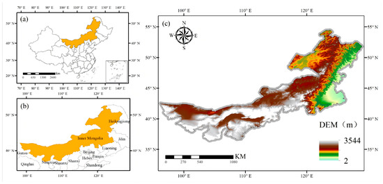
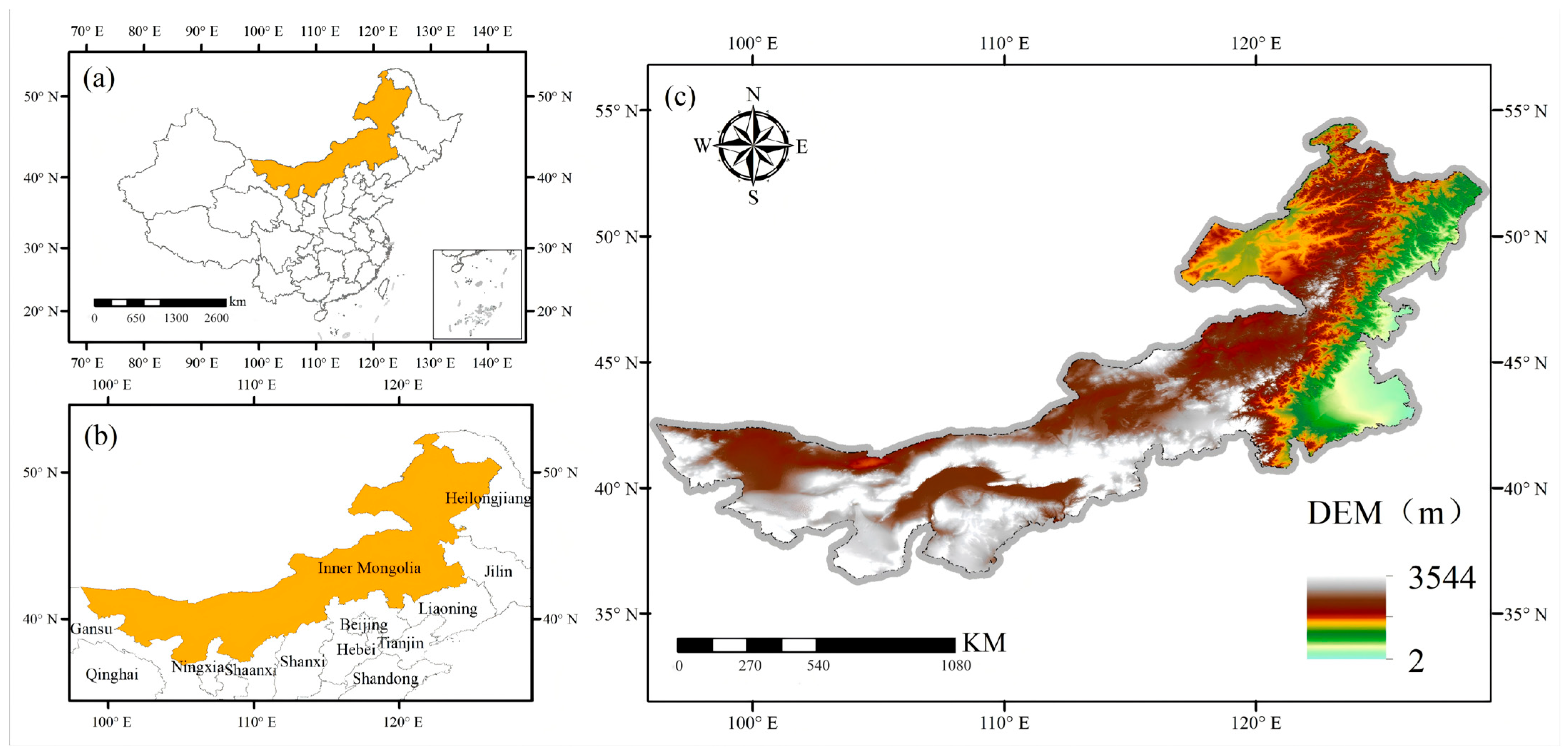
This study takes the Inner Mongolia Autonomous Region as the study area. Inner Mongolia is located in northern China and belongs to the temperate arid/semi-arid zone, with a geographic extent of 97°12′–126°04′ E and 37°24′–53°23′ N and an area of approximately 1.18 million km2. The mean elevation is about 1000 m, and the region is characterized by a large east–west span and marked topographic heterogeneity (Figure 1). The Greater Khingan Mountains in the east, the Yinshan Mountains in the central part, and the Helan Mountains in the southwest together form the topographic framework of the region, and landforms include deserts, mountains, plains, sandy lands, and basins. The study area lies on the margins of the monsoon zone and exhibits monsoon, temperate continental, and plateau climatic characteristics, with annual precipitation of 40–450 mm decreasing from east to west; annual precipitation in the northeast can exceed 400 mm, whereas in the western part it is less than 200 mm, resulting in pronounced differences in available water across the region. Forests and meadow steppe dominate in the east, typical steppe occurs in the central part, and vegetation transitions gradually westward to desert steppe and sandy desert. Over recent decades, ecological programs such as the Grain-for-Green Project and the Three-North Shelterbelt Program have been implemented successively, together with ongoing changes in climate, land use, and vegetation cover, which have exerted noticeable effects on regional water cycling and water yield patterns.
Figure 1.
Location and topography of the study area. (a) Location of Inner Mongolia (highlighted) within China. (b) Inner Mongolia and neighboring provinces (highlighted). (c) Digital elevation model (DEM) of the study area.
2.2. Data Preparation
Based on data availability and the required study period, time-series raster data for 2001–2024 were collected. For InVEST(3.12) simulation, precipitation [27], land-use data [28], and potential evapotranspiration [29] were obtained; for driver analysis, air temperature [27] and NDVI [30] were collected. Most original raster datasets were at monthly resolution and were processed into annual products according to variable type: precipitation and potential evapotranspiration were aggregated as annual totals, air temperature as annual means, and NDVI and FVC as annual maxima.
In addition, soil-texture data were collected to calculate plant-available water content, and 100 m resolution bedrock-depth data [31] were used to determine the depth of the root-restricting layer. GLEAM annual AET products [25,26] were obtained to assist in validating the spatial pattern of simulated evapotranspiration, and a DEM together with derived slope and aspect were used for topographic-factor analysis. All rasters were projected to the Albers equal-area coordinate system, resampled to 1 km to reduce the impact of resampling on raster accuracy, and extracted using the study-area boundary. The names, sources, and resolutions of all datasets are listed in Table 1; biophysical parameters such as Kc and root depth were assigned by land-use type (Table 2).
Table 1.
Data sources, spatial and temporal settings, and use in this study.
Table 2.
InVEST biophysical parameters by reclassified land-use type.
Annual land-use products were preprocessed to integer codes 1–6. Land-use types with very small areal shares and similar eco-hydrological functions were merged into six broad classes: cropland, forest, grassland (including shrubland), water (including ice/wetland), barren land, and built-up land, ensuring that InVEST simulation and XGBoost–SHAP analysis used the same land-use classification. Biophysical parameters for the six land-use types (Kc, root depth, LULC_veg) were set according to InVEST Annual Water Yield module requirements (Table 2). Parameter values refer to the InVEST User’s Guide [24] and similar studies in Northeast China, North China, and the Yellow River Basin [32,33].
2.3. Methods
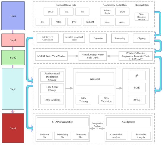
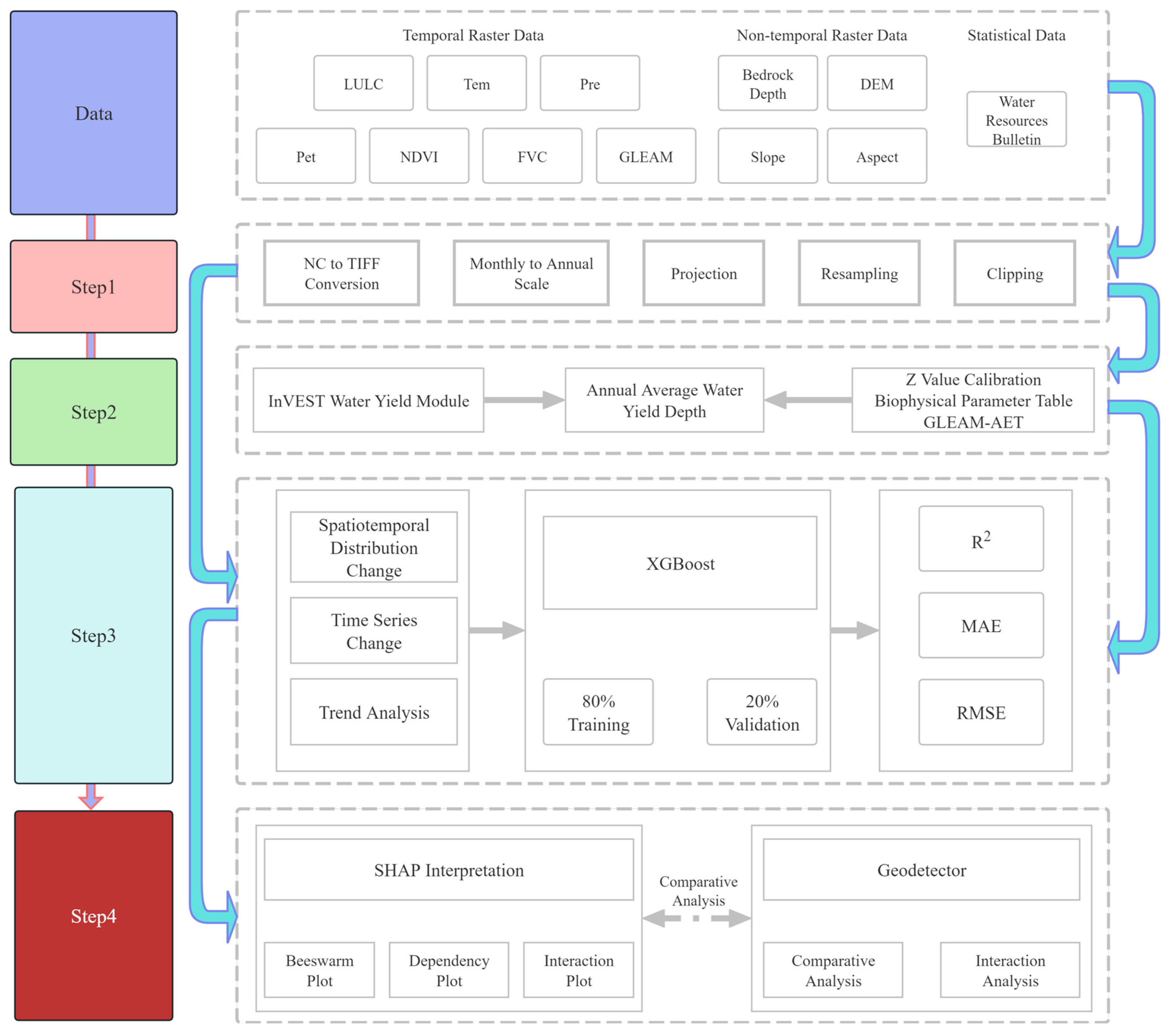
This study simulated water yield depth using the InVEST model, analyzed spatiotemporal changes, and examined nonlinear relationships among driving factors. The technical framework is shown in Figure 2.
Figure 2.
Technical framework of this study.
2.3.1. InVEST Model
This study applied the InVEST annual water yield module [24] to estimate pixel-scale annual water yield depth for 2001–2024. Input data are listed in Table 1; Kc, root depth, and other parameters for each land-use type are given in Table 2; plant-available water content was extracted from HWSD [30]. All rasters were resampled to a common grid, projected, and clipped to the study area before year-by-year model runs.
Annual water yield depth for land-cover class i on pixel x is defined from the water balance as follows:
where Yxi is annual water yield depth (mm yr−1); AETxi is actual evapotranspiration (mm yr−1); and Px is annual precipitation (mm yr−1).
where Kc,x is the evapotranspiration coefficient; ET0x is reference evapotranspiration (mm yr−1); and wx is an empirical parameter from Equation (3).
where Z is the Zhang seasonal factor (dimensionless); MaxSoilDepthx is maximum soil depth (mm); RootDepthx is vegetation root depth (mm); PAWCx is plant-available water content (dimensionless fraction) from Equation (4); and Px is annual precipitation (mm yr−1).
where sand%, silt%, clay%, and OM% are the mass fractions (%) of sand, silt, clay, and organic matter in the soil, respectively; PAWC is the plant-available water content used in Equation (3).
2.3.2. Sen–MK Trend Analysis
Based on pixel-scale annual water yield depth for 2001–2024, Sen’s slope was used to estimate the magnitude of change over time, and the Mann–Kendall test [10,11] was applied to assess trend significance. Sen’s slope is obtained as the median of pairwise annual change rates and is insensitive to individual extreme dry or wet years, making it suitable for Inner Mongolia where interannual water yield variability is large. The Mann–Kendall test is a nonparametric method that does not require a specific distribution and can be computed pixel by pixel for long raster time series. Using annual water yield depth at each valid pixel, and at significance level α = 0.05, trends were classified into five categories: significant increase, non-significant increase, no trend, non-significant decrease, and significant decrease. Trend maps were produced to identify relatively stable and relatively changing areas of water yield.
2.3.3. Geodetector Analysis
Annual water yield depth was used as the dependent variable. Precipitation, potential evapotranspiration, air temperature, NDVI, FVC, topography, and land-use type were selected as independent variables for geodetector analysis [12,34] in selected characteristic years. The method first stratifies pixels by each factor and examines whether annual water yield depth differs significantly among strata; the q statistic indicates the explanatory power of a factor for spatial differentiation in water yield. No predefined linear functional form between independent and dependent variables is assumed. Continuous variables were divided into five strata using sample quintiles; categorical variables were stratified by class. Two steps were conducted: factor detection, calculating q for each factor to compare relative importance; and interaction detection, computing interaction q values for factor pairs to identify weakening, enhancement, or nonlinear enhancement.
2.3.4. XGBoost Model
XGBoost is a gradient boosting ensemble regression method [13] that fits nonlinear relationships between dependent and independent variables by stacking multiple decision trees, and is suitable for pixel-scale multi-factor driver analysis of water yield. For each year from 2001 to 2024, an XGBoost regression model was built with pixel-scale InVEST annual water yield depth as the dependent variable and precipitation, potential evapotranspiration, air temperature, NDVI, FVC, elevation, slope, aspect, and land-use type as independent variables. Land-use type was one-hot encoded into six 0–1 variables and entered the model together with continuous predictors. Each year, valid pixels were randomly split into 80% training and 20% testing (random seed 42); models were fitted on the training set and evaluated on the test set. Hyperparameters were set to 100 trees, maximum depth 5, and learning rate 0.1. Models were implemented in Python 3.10 using the xgboost library and fitted independently by year to compare factor effects under different hydroclimatic conditions.
2.3.5. SHAP Interpretation
Based on annual XGBoost models, SHAP (SHapley Additive exPlanations) [14,15] was used to decompose pixel-level water yield predictions into contributions of input features, identifying dominant features, nonlinear responses, and interactions. A random sample of 20,000 valid pixels (random seed 42) was used for beeswarm plots, dependence plots, and global importance ranking based on mean absolute SHAP values on the subsample. Two-factor interaction effects were computed on a subsample of 5000 pixels. Positive SHAP values indicate that a feature increases predicted water yield relative to the model baseline; negative values indicate the opposite, representing positive and negative effects on the dependent variable, respectively. Unlike geodetector, which treats land use as a single factor, one-hot encoded land-use classes (cropland, forest, etc.) appear separately in SHAP outputs.
3. Results
3.1. Water Yield Simulation Accuracy
In the InVEST annual water yield module, the Z coefficient controls the partitioning of precipitation between evapotranspiration and water yield and has a significant effect on regional total water yield. Given large interannual differences in hydroclimatic conditions in the arid and semi-arid environment of Inner Mongolia, default model parameters cannot ensure basin-wide water balance. Therefore, in each annual InVEST simulation, Z was calibrated against regional water resources reported in the Inner Mongolia Water Resources Bulletin [21]: starting from Z = 1.5, simulated volume was compared with bulletin values after each run; Z was decreased if simulated output exceeded the bulletin and increased if it was lower, with iterative adjustment and re-runs until relative bias was less than 1% [35]. Regional total water yield was therefore in good agreement with official statistics; calibrated Z ranged from 1.21 to 3.34 across years.
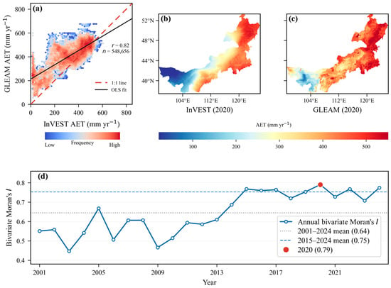
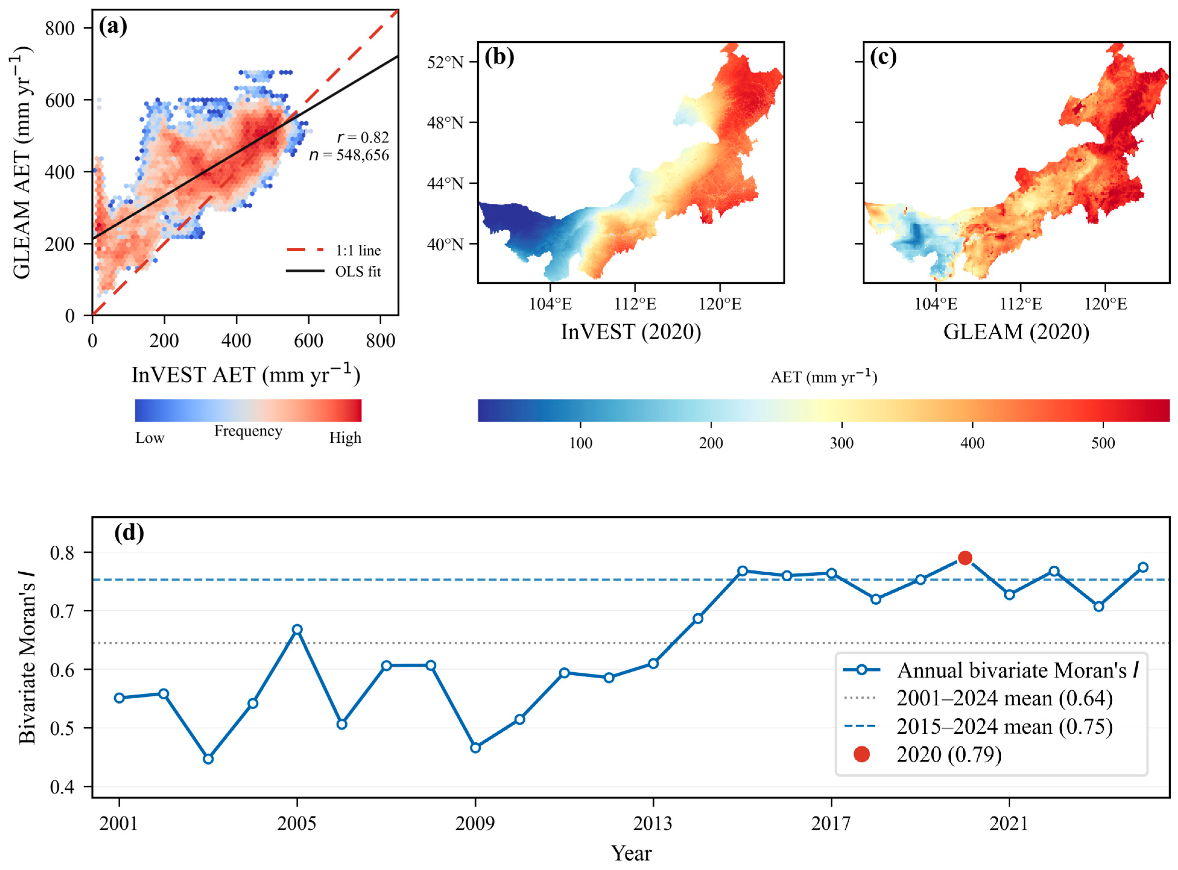
When direct pixel-scale water yield observations are unavailable, evapotranspiration products can be used for indirect evaluation. GLEAM AET [25,26] was used to assess the spatial distribution accuracy of pixel AET rasters exported during InVEST runs, thereby evaluating the spatial plausibility of water yield simulation (Figure 3). Both products were extracted at 2 km grid nodes across the study area; about 550,000 valid pixels were available for 2001–2024. Mean Pearson r was 0.68, with a maximum of 0.82 in 2020, indicating good spatial consistency between the two products. Bivariate Moran’s I [9] showed strong spatial coupling between InVEST AET and GLEAM AET, with a mean bivariate Moran’s I of about 0.64 for 2001–2024 and about 0.75 for 2015–2024; the maximum was 0.79 in 2020. Because independent water-yield observations were unavailable, the GLEAM AET comparison was used only as an indirect check of spatial plausibility in the simulated water-balance components, not as a direct validation of pixel-scale water-yield depth. Overall, the comparison supports the spatial plausibility of the simulated water-balance components, but direct validation of pixel-scale water-yield depth remains unavailable.
Figure 3.
Validation of spatial distribution accuracy between InVEST and GLEAM AET. (a) Scatter plot of pixel-scale InVEST versus GLEAM AET in 2020 (r = 0.82, n = 548,656); dashed red line, 1:1 line; solid black line, OLS fit. (b) Spatial distribution of InVEST AET in 2020. (c) Spatial distribution of GLEAM AET in 2020. (d) Annual bivariate Moran’s I between InVEST and GLEAM AET, 2001–2024.
3.2. Spatiotemporal Patterns of Water Yield Depth
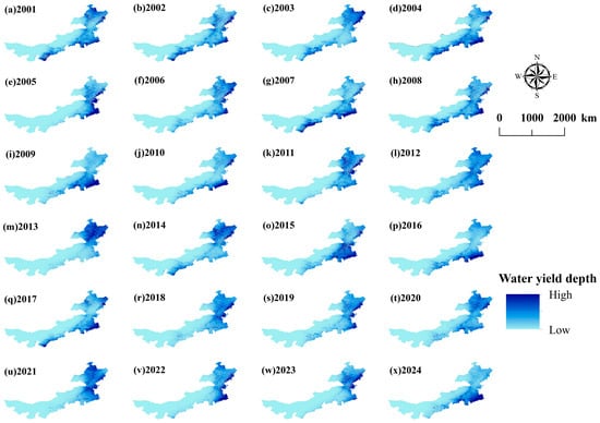
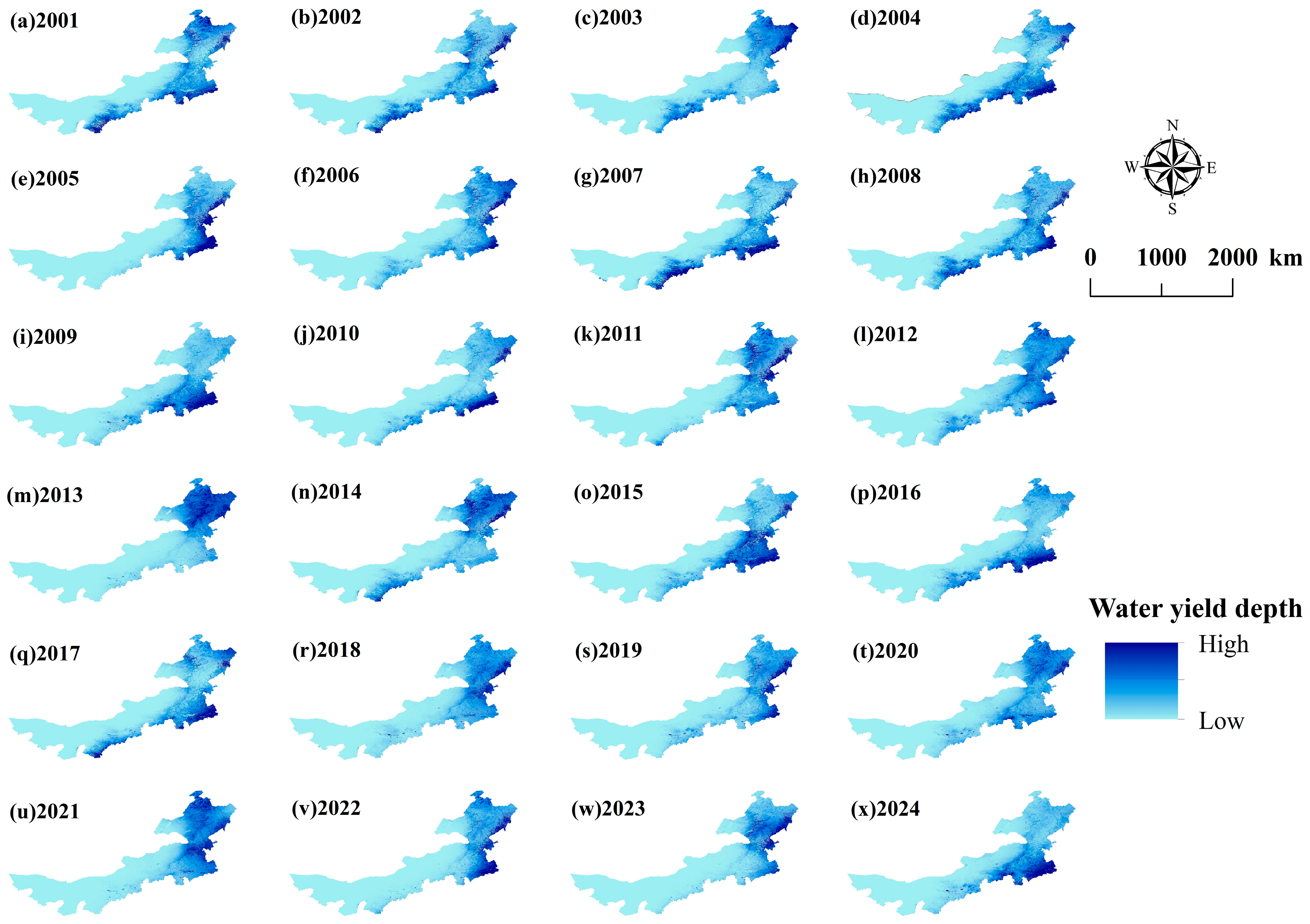
In this study, the study area was divided into eastern, central, and western regions using 115° E and 105° E as boundaries: the western region (X < 105° E), the central region (105° E ≤ X < 115° E), and the eastern region (X ≥ 115° E). The spatial distribution of annual water yield depth from 2001 to 2024 (Figure 4) showed an overall pattern of higher values in the east, lower values in the west, and a transitional zone in the center. The western region accounted for 15.6% of the area, with a multi-year mean water yield depth of only 0.03 mm, contributing almost nothing to total regional water yield. The central region accounted for 29.8% of the area, with a multi-year mean water yield depth of 7.12 mm. The eastern region accounted for 54.6% of the area, with a mean water yield depth of 37.23 mm and a median of 34.38 mm, accounting for more than 90% of regional water yield and serving as the core water yield zone of the region. In terms of spatial configuration, high- and low-yield areas were not scattered in a patchy pattern but extended southwestward along the Greater Khingan Mountains, transitioning through the central plateau to the sandy lands and Gobi Desert in the west, forming a band-like, continuous distribution. The large-scale spatial pattern of water yield depth in Inner Mongolia remained relatively stable over the 24-year period. This spatial distribution pattern was related to the differentiation of hydrothermal conditions, land cover change, topographic and geomorphic differences, and vegetation cover patterns in the study area [18,36].
Figure 4.
Multi-year (2001–2024) mean WY depth spatial map.
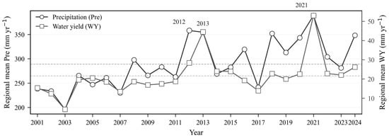
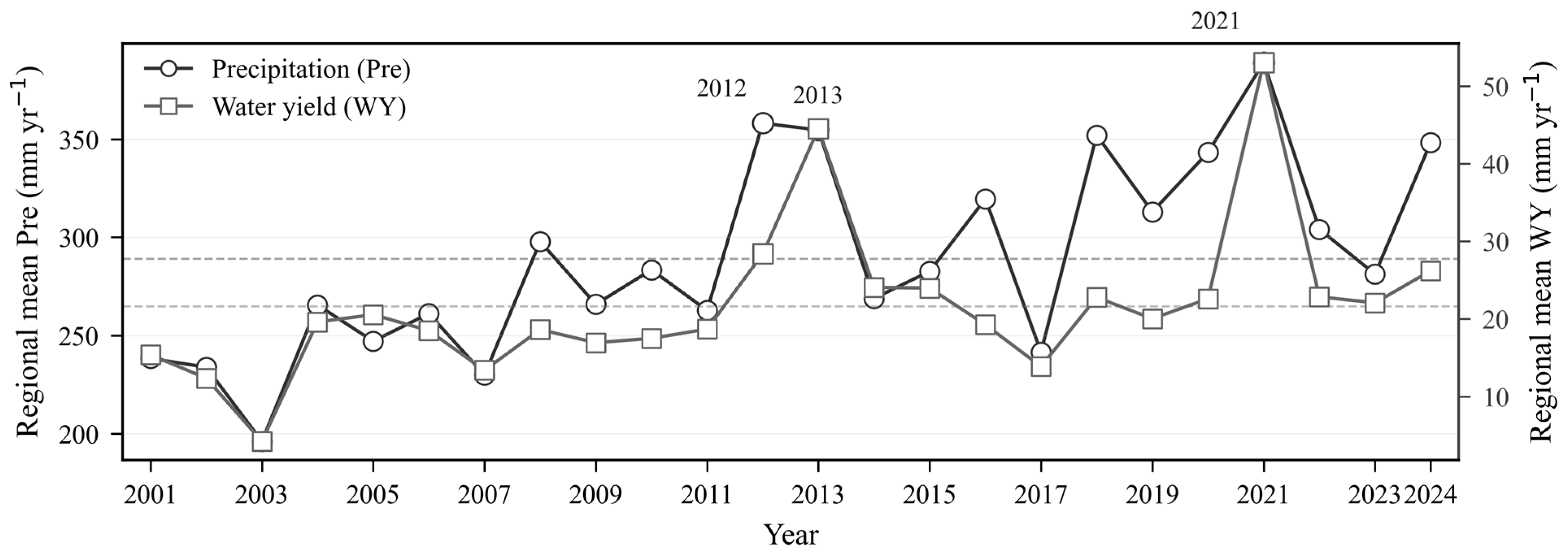
From 2001 to 2024, mean water yield depth in Inner Mongolia showed a fluctuating upward trend (Figure 5). The multi-year regional mean was 22.4 mm yr−1, with water yield depth ranging from 13.4 mm yr−1 (2007) to 53.1 mm yr−1 (2021). Over the same period, the multi-year regional mean precipitation was 295.7 mm yr−1, with precipitation ranging from 230.0 mm yr−1 (2007) to 388.8 mm yr−1 (2021). Regional water yield depth exhibited a slow upward trend amid interannual fluctuations. Mean precipitation depth and water yield depth followed broadly similar temporal patterns. Previous studies have indicated that precipitation is an important controlling factor of water yield [3,4,32,33], and it was positively correlated with water yield.
Figure 5.
Interannual regional mean precipitation (Pre) and water yield (WY) in Inner Mongolia, 2001–2024.
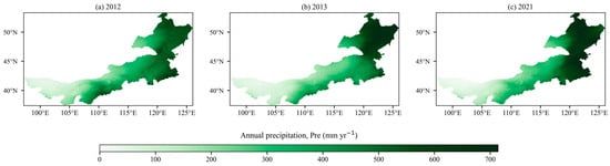
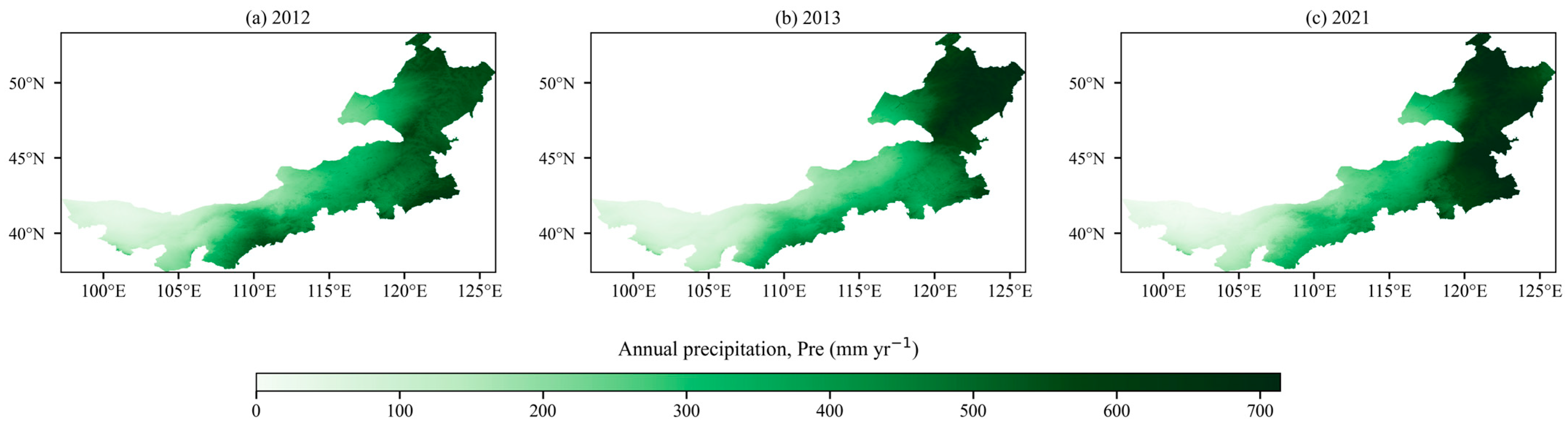
Figure 5 similarly shows that, when comparing 2012 with 2013, water yield depth was relatively lower in 2012 despite its higher precipitation. As seen in Figure 6, this may be related to the spatial distribution of precipitation. Regional mean precipitation depth in 2012 and 2013 was similar, at 358.1 mm yr−1 and 354.8 mm yr−1, respectively; in 2012, the central region received 299 mm yr−1 and the eastern region 467 mm yr−1, whereas in 2013 precipitation in the central region decreased to 233 mm yr−1 and in the eastern region increased to 503 mm yr−1. In wet years such as 2013 and 2021, precipitation was concentrated in the high-yield eastern zone, whereas in 2012 precipitation was also relatively concentrated in the central region. Such spatial differentiation in precipitation contributed, to some extent, to changes in regional mean water yield depth. Therefore, a comprehensive understanding of the driving factors affecting the spatial distribution of water yield is needed.
Figure 6.
Spatial distribution of annual Pre in 2012, 2013 and 2021.
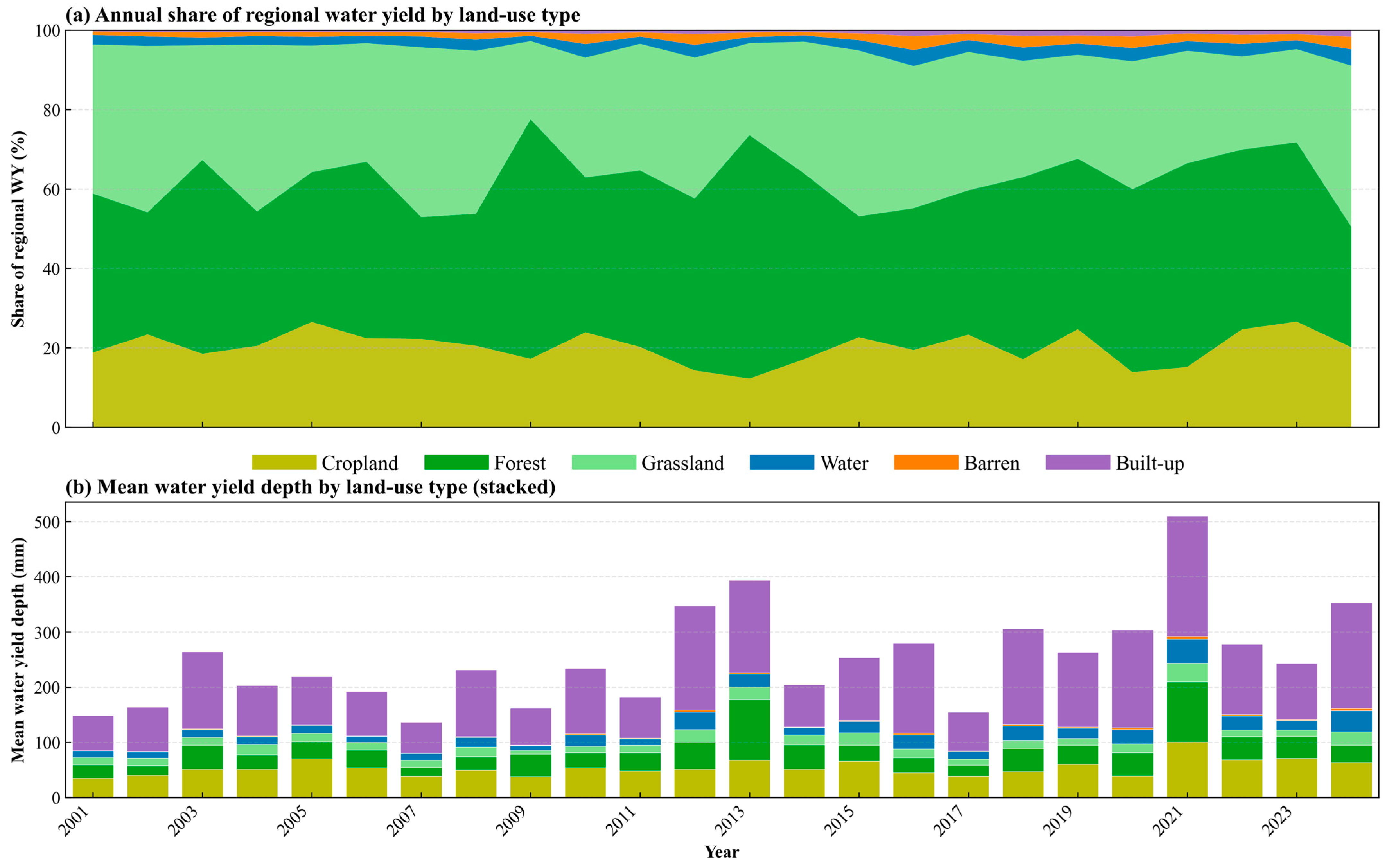
In terms of land-use effects on water yield, forest, grassland, and cropland together accounted for about 95% of regional total water yield from 2001 to 2024 (Figure 7). Water bodies, barren land, and built-up land together accounted for less than 5% in most years. The share of forest water yield increased markedly in wet years, e.g., about 61% in 2013 and about 51% in 2021, indicating that wet-year water yield was mainly contributed by forests in the northeast and east. In drier years, the grassland share increased relatively, e.g., about 43% grassland and about 31% forest in 2007; cropland contributed about 18–27% and was a stable secondary source. In mean water yield depth by class, built-up land was highest, but its areal share was small, so its effect on regional total water yield was negligible. Mean water yield depth for cropland and forest pixels was generally higher than for grassland and barren land; class means rose and fell with wet and dry years, in phase with the regional mean. Barren land remained low throughout, corresponding to western sandy desert areas. In summary, the eastern high-yield belt was associated with higher forest and cropland shares and intensities in wet years, whereas the western low-yield pattern was maintained by extensive grassland and persistently low-yield barren land; mean water yield depth of grassland increased slightly in dry years.
Figure 7.
Land-use contributions to regional water yield, 2001–2024. (a) Annual share (%) of regional total by land-use class. (b) Mean pixel water-yield depth (mm yr−1) by land-use class.
3.3. Trend Analysis of Water Yield Depth
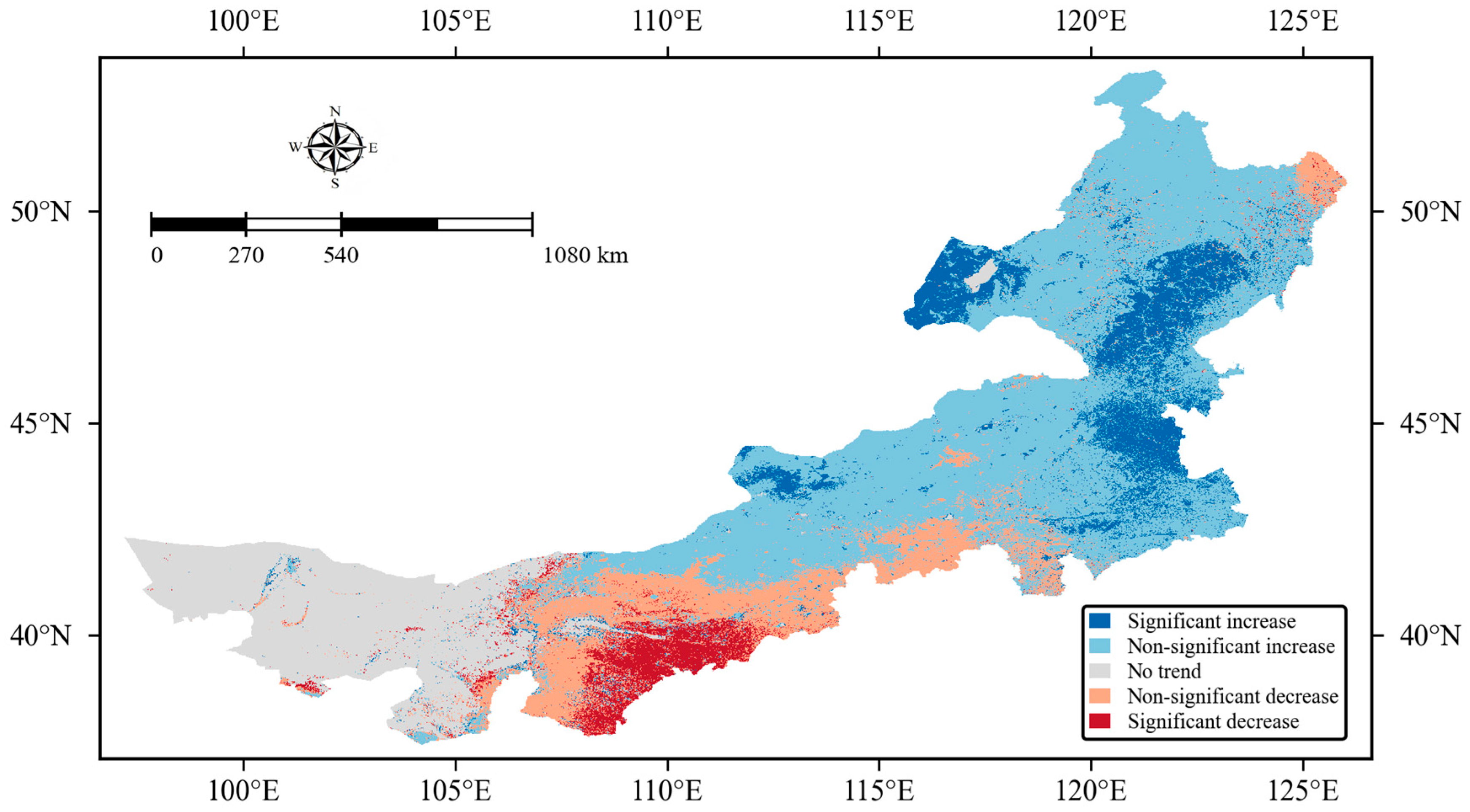
Sen’s slope combined with the Mann–Kendall test [10,11] (α = 0.05) was applied to pixel-scale annual water yield depth time series for 2001–2024 to classify five trend categories (Table 3; Figure 8). Among valid pixels, non-significant increase accounted for 50.19%, followed by significant increase at 12.35%. No trend, non-significant decrease, and significant decrease accounted for 18.84%, 14.11%, and 4.50%, respectively. Increase classes totaled 62.54% and decrease classes 18.61%. At the regional scale, simulated water yield was more characterized by increase or weak increase rather than widespread significant decrease, consistent with the regional mean change in water yield depth. Significant increase pixels occurred mainly in the northeast, the southeastern piedmont of the Greater Khingan Range, and parts of the eastern steppe, in contiguous patches or clusters near eastern high-yield zones. Significant decrease pixels were limited in area but formed a relatively concentrated zone in the south-central region, surrounded mainly by non-significant decrease pixels. Western and central low-yield areas were dominated by no trend and non-significant change.
Table 3.
Sen–MK trend class area proportions (2001–2024).
Figure 8.
Sen–MK five-class trend map, 2001–2024.
Sen’s slope statistics for significantly changing pixels are summarized in Table 4. For significant increase pixels, the mean was 1.45 mm yr−2 (median 1.26 mm yr−2; interquartile range 0.17–1.87 mm yr−2). For significant decrease pixels, the mean was −1.06 mm yr−2 (median −1.07 mm yr−2; interquartile range −1.52 to −0.57 mm yr−2). Increase pixels were more extensive in area, and mean change rate (absolute value) was slightly stronger than for decrease pixels. The wider interquartile range for increase pixels indicates greater heterogeneity in change rates within significant increase areas, i.e., spatially non-uniform change.
Table 4.
Sen’s slope for significant trend pixels (mm yr−2).
3.4. XGBoost–SHAP Analysis
3.4.1. Model Performance
As shown in Table 5, for each year from 2001 to 2024, 80% of pixels were used for training and 20% for testing. XGBoost showed relatively stable reproduction of InVEST annual water yield depth. Test-set coefficient of determination (R2) ranged from 0.864 to 0.970, with a 24-year mean of 0.911. Multi-year mean root mean square error (RMSE) and mean absolute error (MAE) were 8.86 mm and 3.78 mm, respectively; interannual ranges were 2.41–13.20 mm for RMSE and 0.69–5.25 mm for MAE. In wet, high-yield years (e.g., 2021), R2 was higher, but millimeter-scale errors were also larger (RMSE 13.20 mm, MAE 5.25 mm). In low-yield years (e.g., 2003), errors were correspondingly smaller (RMSE 2.41 mm, MAE 0.69 mm). In 2024, R2 was 0.925, RMSE was 10.98 mm, and MAE was 4.65 mm. Overall, R2 remained above 0.86 in all years, and no obvious failure occurred in dry years (e.g., 2002, 2008). Under the east-high and west-low pattern and marked interannual variability, model fitting accuracy at the pixel scale is sufficient for subsequent driver interpretation.
Table 5.
XGBoost test-set performance by year.
3.4.2. Global Feature Importance
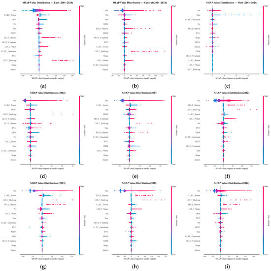
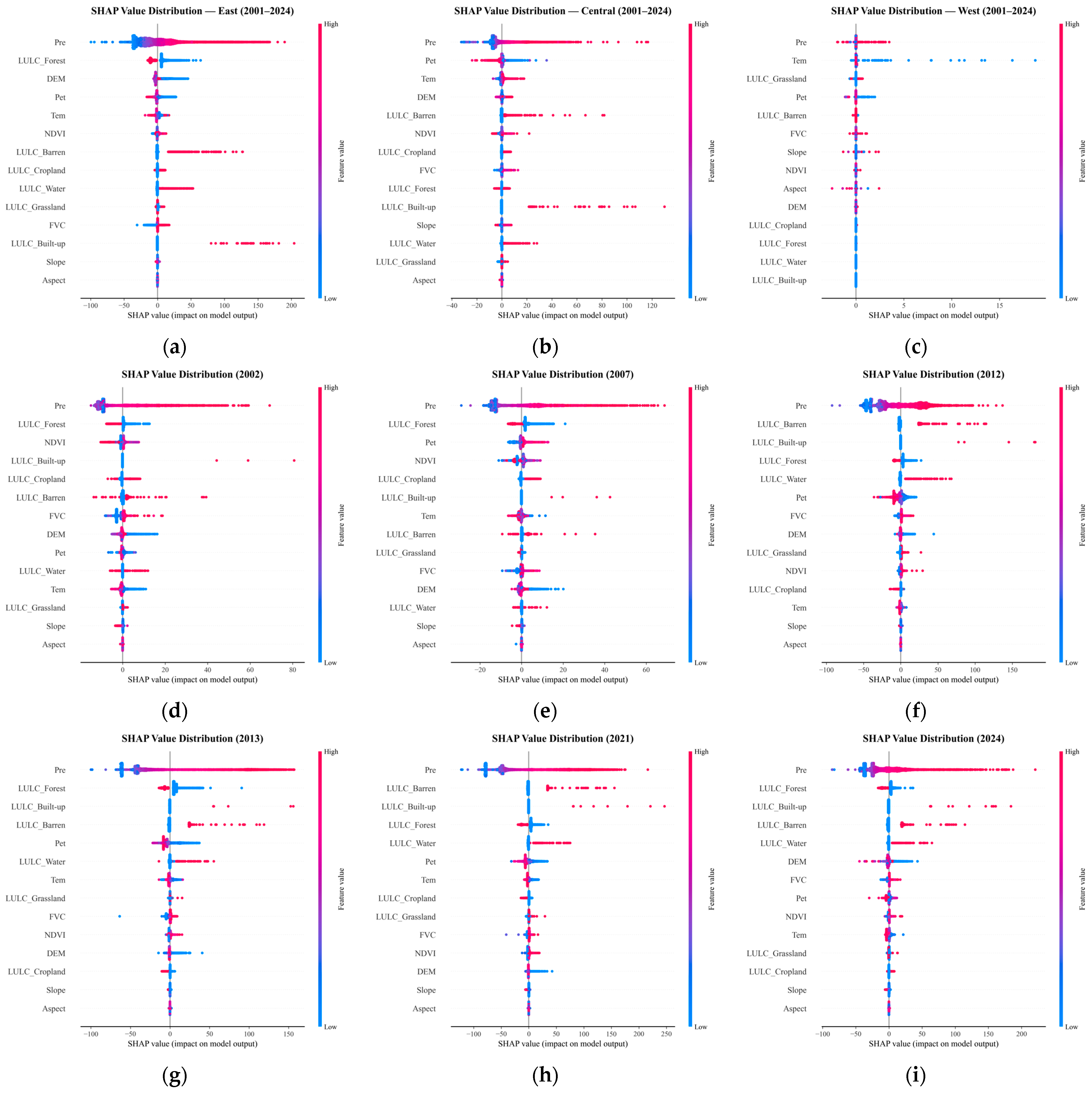
Figure 9a–c presents zonal SHAP analyses based on pooled pixel-year records for 2001–2024. Separate XGBoost models were trained and interpreted for the East, Central, and West zones. The beeswarm plots show that precipitation (Pre) was the leading driver in all three zones, with contribution shares of 48.8%, 63.5%, and 37.7%, respectively. In the East, forest (19.3%) and DEM (8.4%) ranked second. Pre dominance was most pronounced in the Central zone. In the West, where water yield was extremely low and the absolute SHAP magnitudes of all factors were much smaller than in the East and Central zones, temperature (Tem, 32.1%) had a relatively higher share. Because Pre ranked first in all three zones and the East accounted for over 90% of regional water yield, subsequent analyses were conducted at the region-wide scale in Figure 9d–i for six characteristic years to examine temporal variation in driver structure.
Figure 9.
SHAP value distributions of drivers affecting water yield. (a–c) West, Central, and East (2001–2024); (d–i) region-wide characteristic years: 2002, 2007, 2012, 2013, 2021, and 2024.
Figure 9d,e shows SHAP beeswarm plots for 2002, 2007, 2012, 2013, 2021, and 2024. A common feature across all six panels is that the Pre point cloud is widest horizontally and farthest from the vertical axis, whereas most other factors cluster in narrow bands near zero, indicating that pixel-scale water-yield prediction is mainly driven by precipitation. Pre point colors from blue to red correspond to low-to-high feature values: low-precipitation pixels tend to have negative or near-zero SHAP values, and high-precipitation pixels tend to have positive SHAP values, showing clear positive co-variation. In wet years (2013, 2021), the red end of the Pre cloud is longer and more pixels have positive SHAP; in dry years (2002, 2007), the cloud contracts toward the zero axis and negative points increase. Land-use types appear as discrete vertical bars rather than continuous bands, and SHAP can be positive or negative within the same class, indicating that water-yield responses to underlying surface are modulated by precipitation background. In 2012, Pet and barren-land clouds are more dispersed than in other dry/wet years, with both positive and negative SHAP values, consistent with the “precipitation–water yield asynchrony” characteristic of that year. In 2024, forest and barren-land bars have certain width, but both are far narrower than Pre. NDVI, FVC, slope, and aspect point clouds lie almost on the vertical axis, contributing minimally to pixel-level prediction.
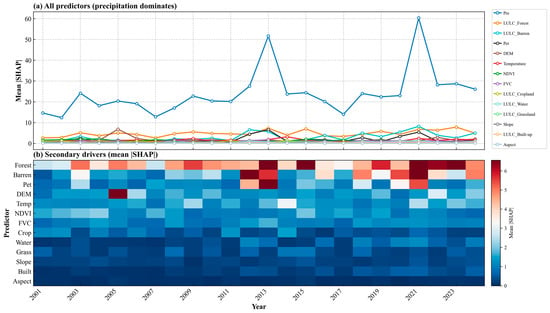
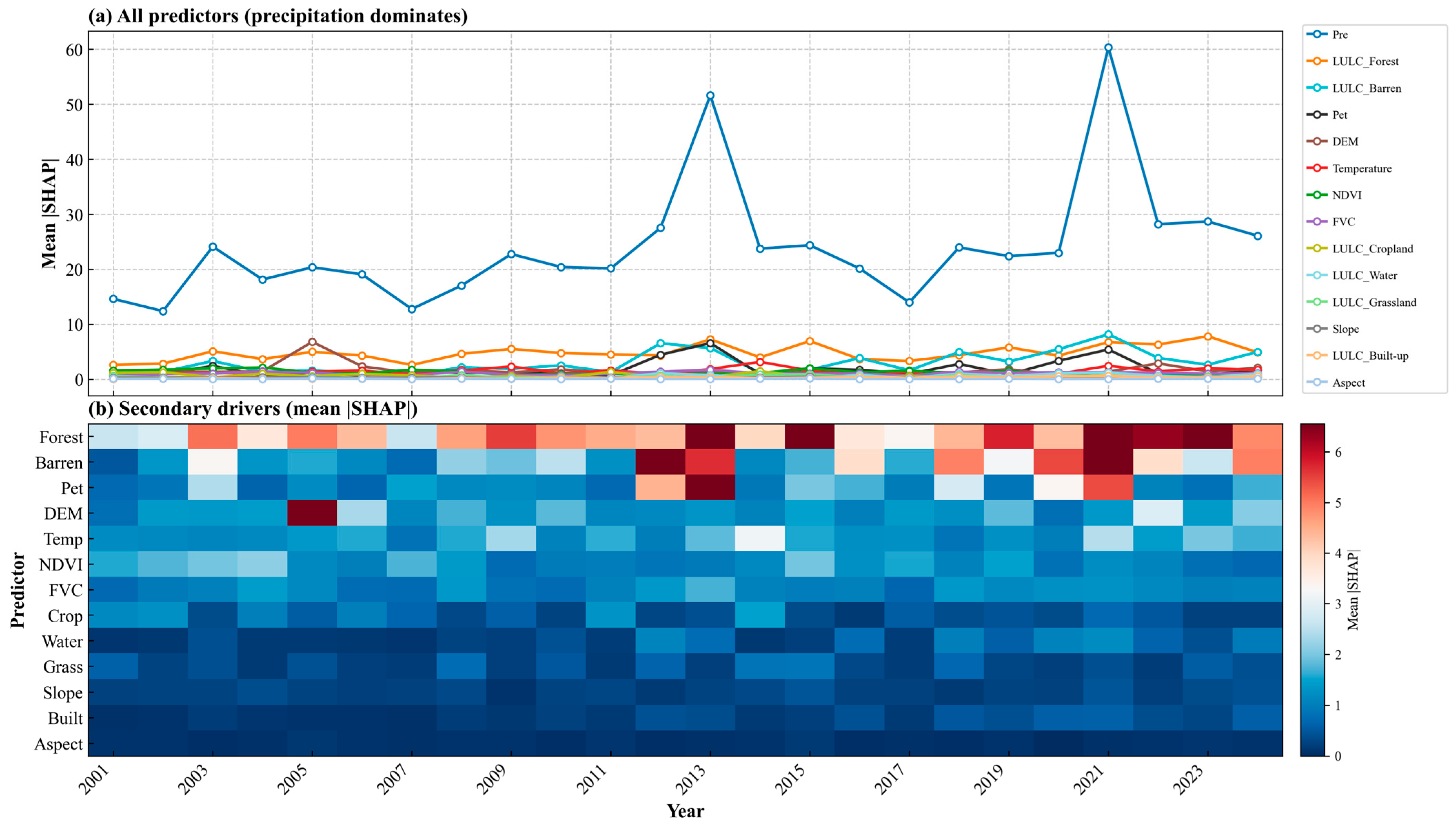
Figure 10a shows the interannual variation in mean |SHAP| for each driving factor from 2001 to 2024. Precipitation’s mean |SHAP| led all other factors by a wide margin in every year. Its contribution share averaged 57.7% over the 24 years, reaching 66.8% in the high year (2021) and 50.7% in the low year (2005). |SHAP| fluctuated between 11.2 and 60.2 mm with interannual precipitation, consistent with the temporal variation in precipitation in the study area; therefore, precipitation is the dominant factor in the spatial differentiation of water yield depth.
Figure 10.
Interannual variation in mean |SHAP| by feature, 2001–2024. (a) All predictors; (b) secondary predictors (precipitation excluded).
Because precipitation’s contribution share in Figure 10a is too large for secondary factors to be seen clearly, Figure 10b presents secondary factors as a heat map to show their interannual variation; the contribution shares of different factors still changed to some extent from year to year. Over the 24-year average, forest (11.7%), barren land (6.7%), elevation (4.3%), potential evapotranspiration (4.1%), and air temperature (3.8%) were the secondary factors with relatively high contributions; NDVI (3.4%) and FVC (2.9%) ranked next; cropland (1.7%), water bodies (1.0%), grassland (1.0%), and built-up land (0.6%) had lower shares; and slope (0.7%) and aspect (0.2%) were almost negligible. Mean |SHAP| for most secondary factors was below 10 mm, so they could not dominate the interannual pattern of water yield spatial differentiation, though both contribution magnitude and contribution share still varied interannually—for example, forest share increased in 2023 and 2015 (up to 16.7%), barren land strengthened in 2012, 2020, and 2024 (10.7–13.1%), and potential evapotranspiration stood out in 2012, 2013, and 2020 (8.0–8.9%). Overall, with precipitation always in the primary position, land cover types (especially forest and barren land) together with topography and evapotranspiration formed the secondary factors in water yield spatial differentiation; the remaining factors contributed limitedly to model predictions and mainly acted as auxiliary influences under specific conditions.
3.4.3. Nonlinear Effects of Predictors
Dependence plots were constructed for one representative continuous predictor from each of four main control dimensions—climate, evapotranspiration, vegetation, and topography—namely Pre, Pet, NDVI, and DEM. The same predictor was compared across six characteristic years (2002, 2007, 2012, 2013, 2021, and 2024), covering dry and wet hydrological conditions and spanning most of the 2001–2024 study period.
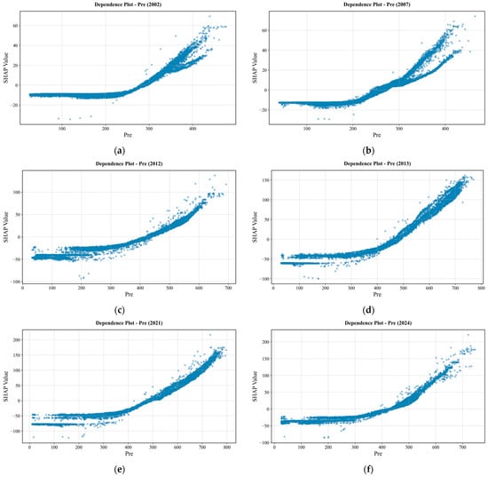
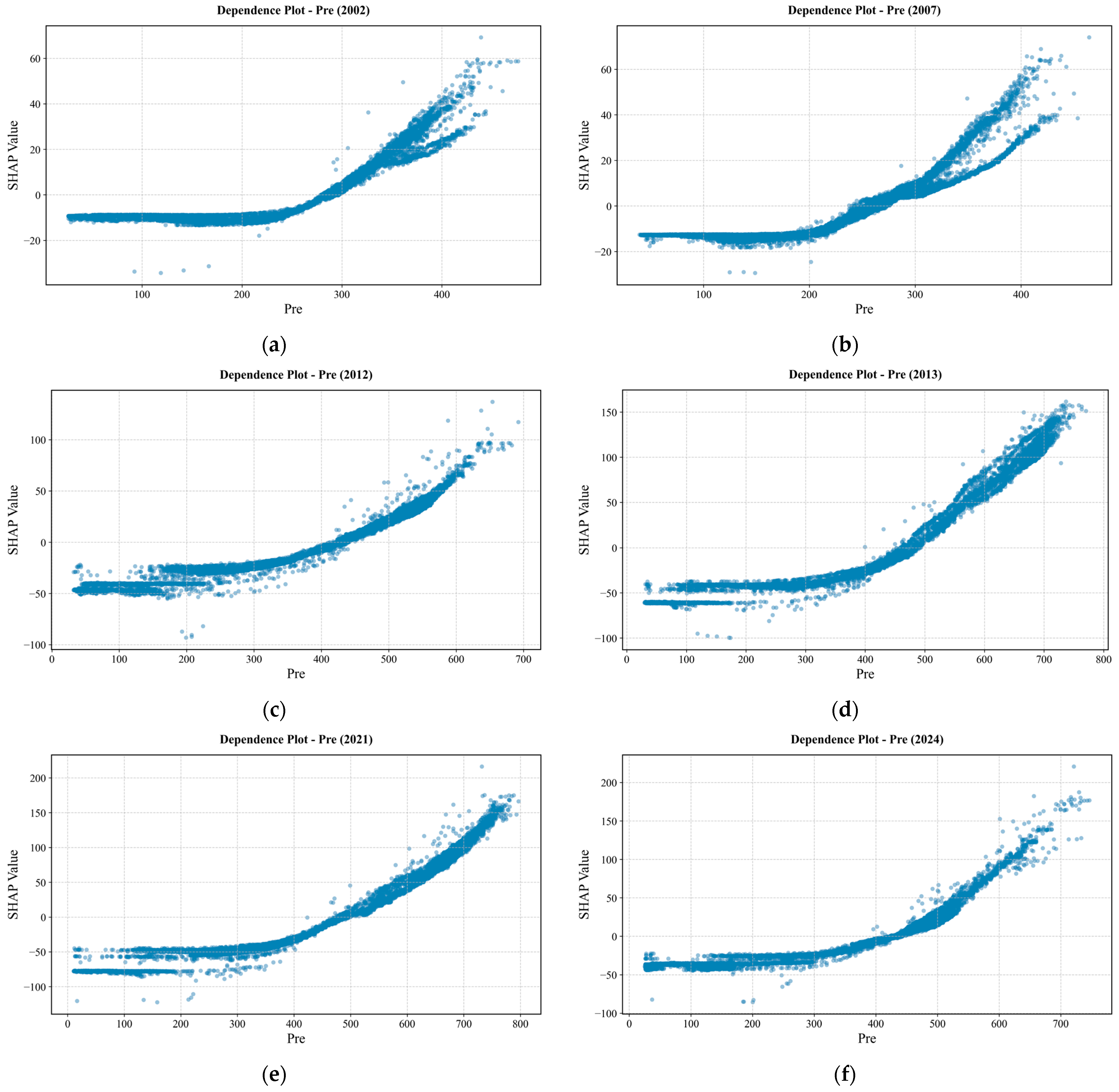
Dependence plots for the six characteristic years show that precipitation exerts a clear segmented influence on water yield (Figure 11). At low precipitation, SHAP values are mostly negative; once precipitation exceeds a certain level, SHAP rises sharply with increasing Pre, with a markedly steeper slope in the high-precipitation segment. Threshold positions and curve shapes differ substantially among years. In 2002 and 2007, regional water yield was low and precipitation was relatively scarce—typical dry years. In both panels, overall Pre SHAP variation is small, inflection points occur earlier, and uplift at high precipitation is limited. In 2007, SHAP at low precipitation is mostly slightly below zero; although values turn positive as precipitation increases, the rate and magnitude of increase are weaker than in wet years. In 2012, 2013, 2021, and 2024—all wet years within the study period—SHAP at low precipitation is lower, SHAP at high-precipitation pixels is higher, and the rear segment of the curve rises more rapidly. In 2021, SHAP at high precipitation reaches the maximum among the six panels. Although regional precipitation in 2012 exceeded that in 2013, the water-yield increase was smaller than in 2013; the dependence inflection occurs further to the right, with marked uplift only near ~400 mm, reflecting asynchronous precipitation–water-yield response in that year. In 2024, precipitation conditions fall between dry and wet years; the tail of the curve still rises noticeably, but regional mean water yield and SHAP intensity are both lower than in 2013 and 2021, providing a recent reference year. In dry years, dependence scatter at high precipitation shows vertical dispersion, indicating that at similar precipitation levels, model response may still be modulated by factors such as land use; this requires further interpretation with interaction plots and spatial analysis.
Figure 11.
SHAP dependence of predicted annual water-yield depth on precipitation (Pre). (a) 2002; (b) 2007; (c) 2012; (d) 2013; (e) 2021; (f) 2024.
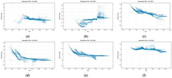
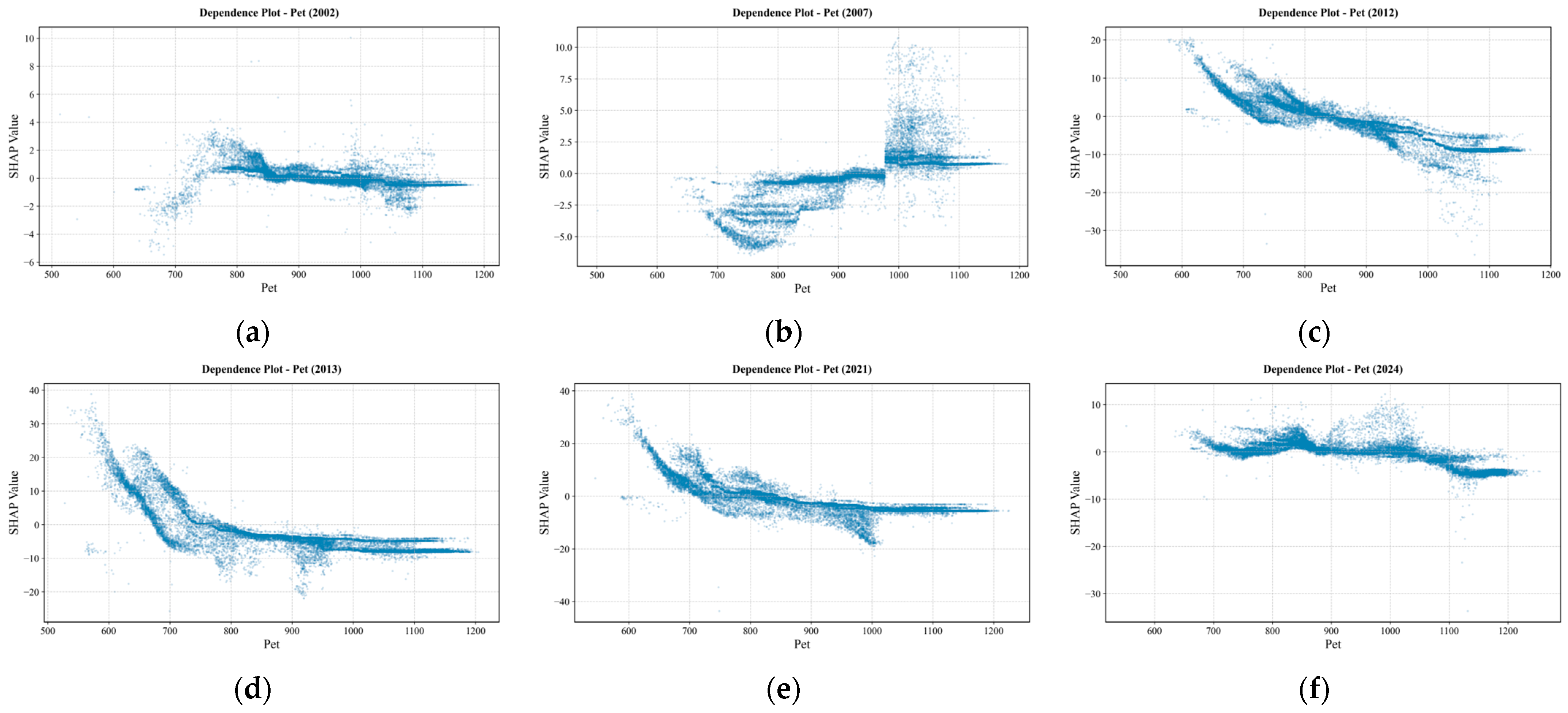
From the Pet and SHAP dependence plots for the characteristic years (Figure 12), it can be seen that in dry years (2002, 2007), the curves mostly lie close to the zero axis; across low, mid, and high Pet segments, no clear, stable upward or downward trend is formed. Although individual pixels show positive or negative outliers, at the regional scale Pet has a weak influence on water yield. In wet years, the patterns are clearer: at low Pet, SHAP is mostly positive; as Pet increases, SHAP declines overall, the positive effect gradually weakens, and in the mid-Pet range it turns from positive to negative; as Pet continues to increase, values mostly remain near negative values or change little. Among these, the decline is larger in 2013 and 2021; the overall trend in 2012 is similar to 2013 and 2021, but the magnitude of change is reduced. In 2024, a negative correlation trend can still be seen to some extent, but the overall influence is likewise weak; as Pet increases, SHAP values vary within the range of 10 to −10. Therefore, in wet years, the model is more inclined to raise water-yield predictions when Pet is low and suppress them when Pet is high; dry years lack the above clear correspondence.
Figure 12.
SHAP dependence on potential evapotranspiration (Pet). (a) 2002; (b) 2007; (c) 2012; (d) 2013; (e) 2021; (f) 2024.
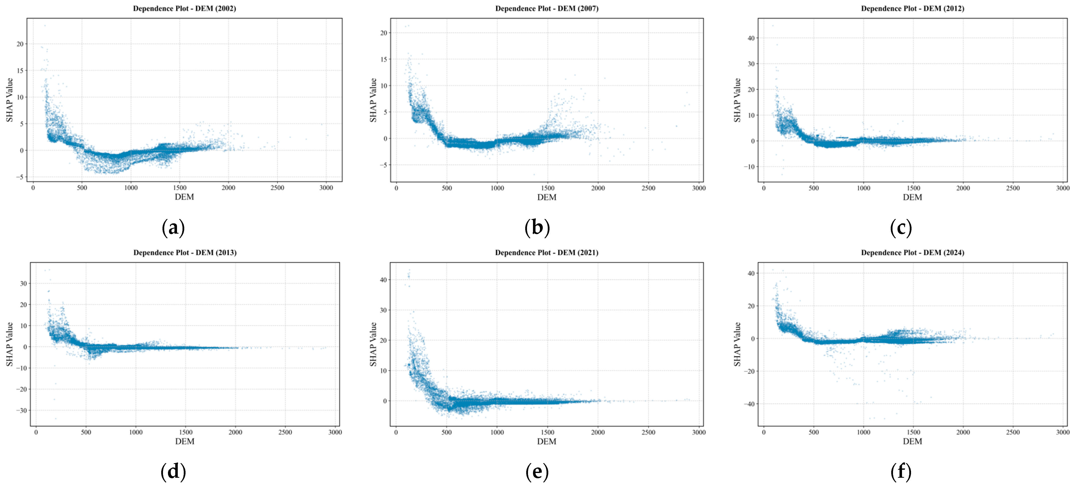
Figure 13 shows the SHAP dependence plots for DEM. The scatter points are mainly concentrated in elevation zones below 2000 m, whereas areas above 2000 m account for a relatively small proportion. Across all years, the trend is that SHAP values gradually weaken with increasing elevation. Below 500 m, SHAP values are mostly positive, indicating a positive contribution. Above 500 m, SHAP values mostly fluctuate around zero and do not continue to decline into a sustained negative contribution, indicating that the effect of elevation on water yield depth is mainly concentrated in mid–low elevation zones, and wet and dry years do not exhibit clear threshold-like turning points. This suggests that topography acts more as a supplementary regulating mechanism in the water yield pattern of Inner Mongolia, and its interannual variation is relatively small.
Figure 13.
SHAP dependence on digital elevation model (DEM). (a) 2002; (b) 2007; (c) 2012; (d) 2013; (e) 2021; (f) 2024.
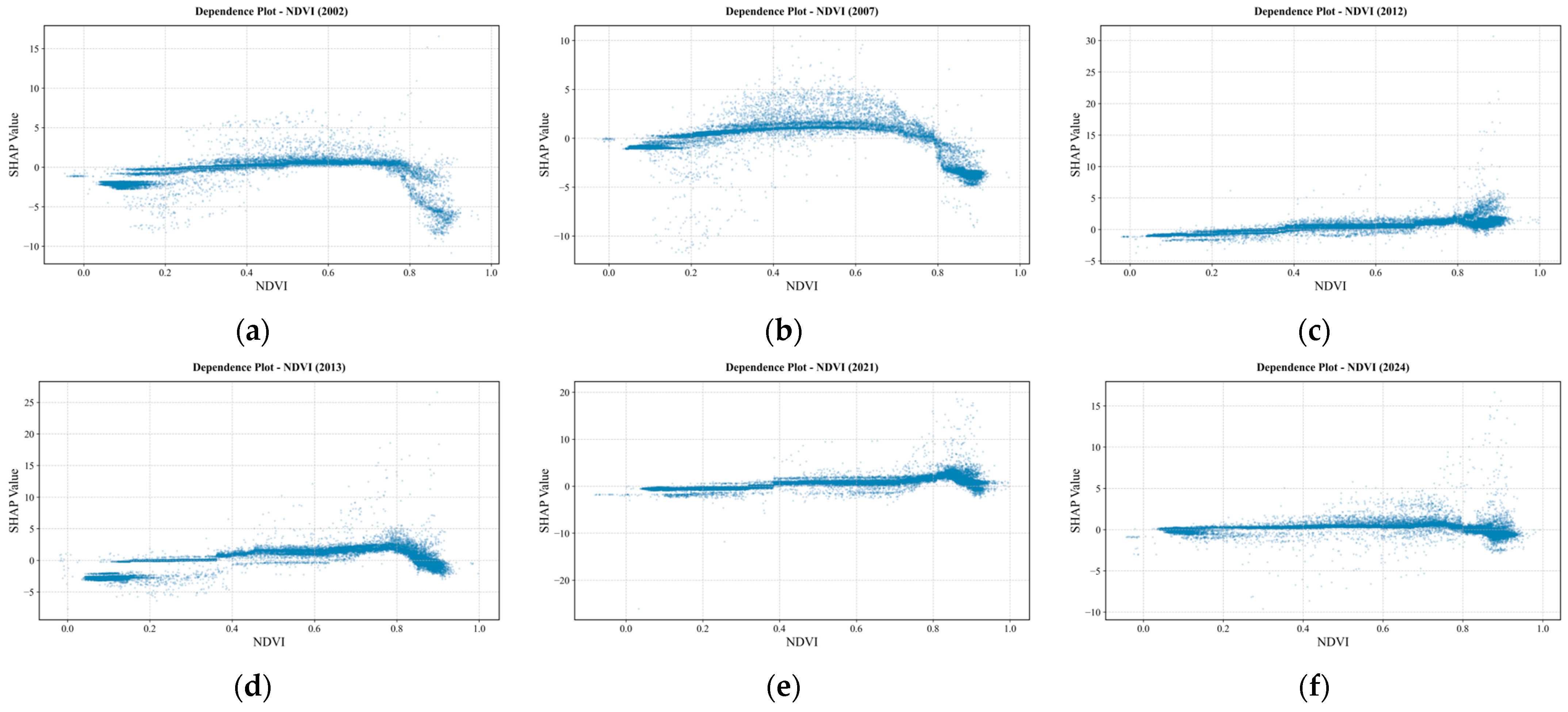
Figure 14 shows the SHAP dependence plots for NDVI in selected years. Compared with climatic and topographic factors, NDVI consistently ranked as a secondary factor in the annual importance ordering. The dependence plots show that most scatter points cluster near the zero axis of SHAP, indicating that the vegetation index plays a supplementary regulating role in water yield prediction. Comparing wet and dry years, dry years (2002 and 2007) exhibit an arch-shaped distribution near the zero axis, with SHAP values generally low at both low and high NDVI; in the middle range (0.4–0.6), SHAP values for some pixels rise above the zero axis, indicating a slight positive effect on predicted water yield depth under moderate vegetation cover. Wet years mostly show a flat distribution near the zero axis, and changes in NDVI lead to limited variation in water yield prediction. In some years, scatter points spread upward at NDVI > 0.8 or a few higher outliers appear, but the main body of points still remains close to the zero axis; therefore, this pattern should not be generalized to the entire study area.
Figure 14.
SHAP dependence on normalized difference vegetation index (NDVI). (a) 2002; (b) 2007; (c) 2012; (d) 2013; (e) 2021; (f) 2024.
In summary, for precipitation, dependence-plot shapes are not consistent among years: in dry years (2002, 2007), overall variation is small, SHAP in low- and mid-precipitation segments fluctuates mostly near or below the zero axis, uplift at high precipitation is limited, and vertical dispersion appears; in wet years, SHAP at low precipitation is relatively lower, uplift with increasing Pre is more pronounced, uplift at high precipitation is clear, and vertical dispersion is absent. For topography, interannual dependence plots are broadly similar: below ~500 m SHAP is mostly positive, weakening with elevation and turning from positive to negative; above 1000 m values approach zero, and differences in water-yield prediction concentrate mainly in mid- to low-elevation bands. For potential evapotranspiration, in dry years scatter points mostly lie close to the zero axis; in wet years SHAP declines with increasing Pet and turns from positive to negative, and at high Pet values are mostly negative with limited further change. For NDVI, the influence is clearly weaker than Pre, Pet, and DEM; dry years often show arch-shaped distributions near the zero axis, whereas wet years mostly show flat distributions.
3.4.4. Interactions Among Predictors
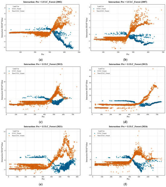
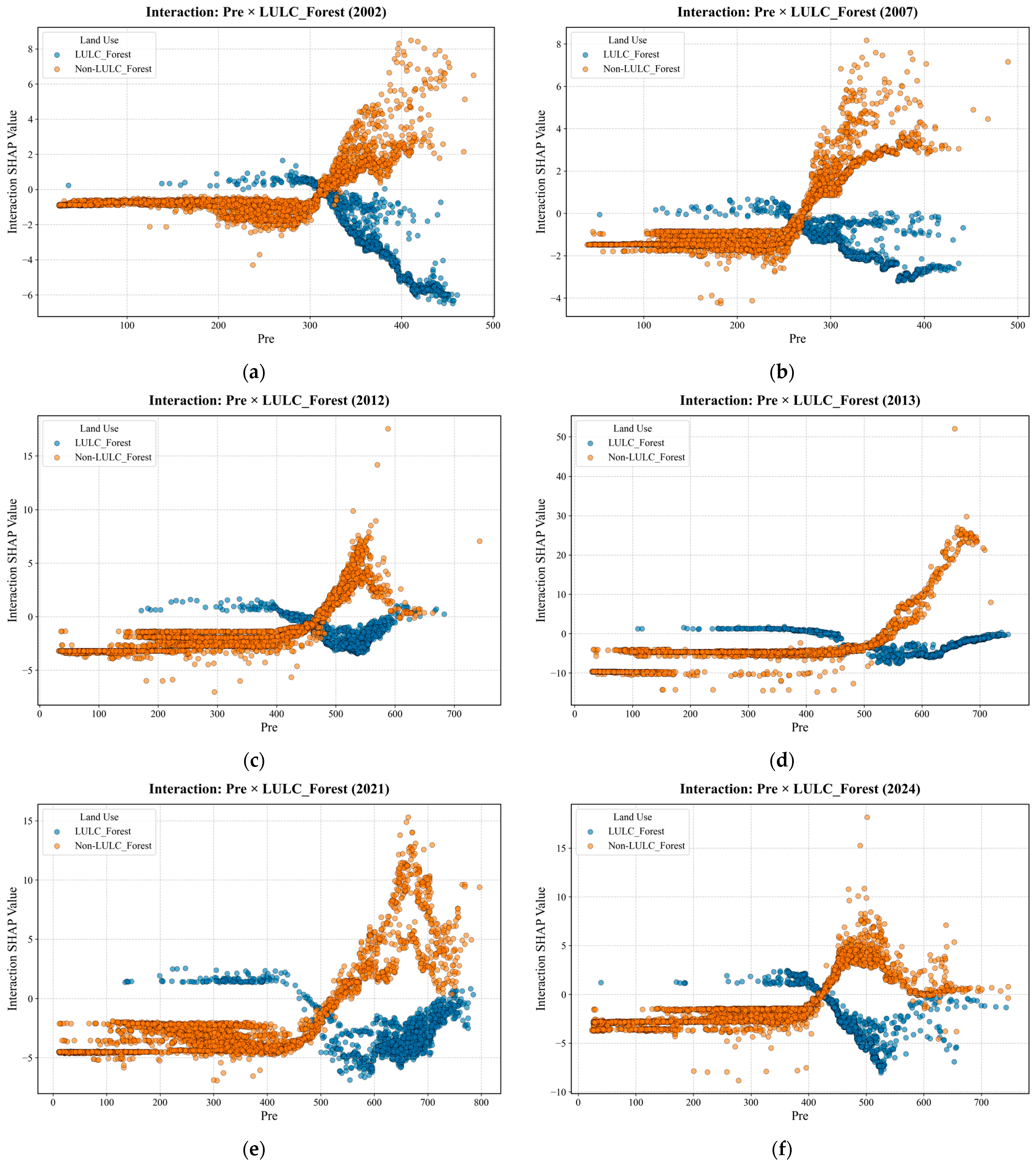
Distinguished by dry and wet years, six characteristic years (2002, 2007, 2012, 2013, 2021, and 2024) were selected for SHAP interaction analysis of two factor pairs: precipitation versus forest land, and precipitation versus potential evapotranspiration. Precipitation was the primary factor in all years; forest modulation was especially pronounced under high-rainfall conditions, and the precipitation–forest interaction was generally the strongest across years. Pre × Pet was also significantly enhanced in some dry and wet years. The two pairs correspond to the joint effects of “precipitation–underlying surface” and “precipitation–evapotranspiration background,” respectively.
SHAP interaction plots for precipitation and forest land (Figure 15). Interaction values represent the extra contribution to water-yield prediction under the combined effect of precipitation and forest versus non-forest status—the portion beyond the sum of their main effects. As can be seen from the figure, in the low- to mid-precipitation range, interaction values for forest and non-forest land with precipitation change relatively smoothly and cluster near the zero axis, indicating that when precipitation is low, synergistic differences between forest and non-forest land with precipitation are small. When precipitation exceeds a certain threshold, non-forest interaction values mostly rise rapidly to positive values, whereas forest values mostly remain near the zero axis or turn negative; the scatter distributions for forest and non-forest land show a “scissor” pattern, indicating that under high-precipitation conditions, the model attributes more water-yield uplift to positive synergy between non-forest land and precipitation. On forest pixels, the extra uplift from high precipitation is relatively weak, and even negative interaction may occur, consistent with the understanding that forest land has stronger evapotranspiration and interception. The transition point for forest–non-forest synergistic interaction occurs at 200–300 mm in dry years and mostly at 400–500 mm in wet years.
Figure 15.
SHAP interaction of Pre and LULC_Forest. (a) 2002; (b) 2007; (c) 2012; (d) 2013; (e) 2021; (f) 2024.
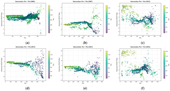
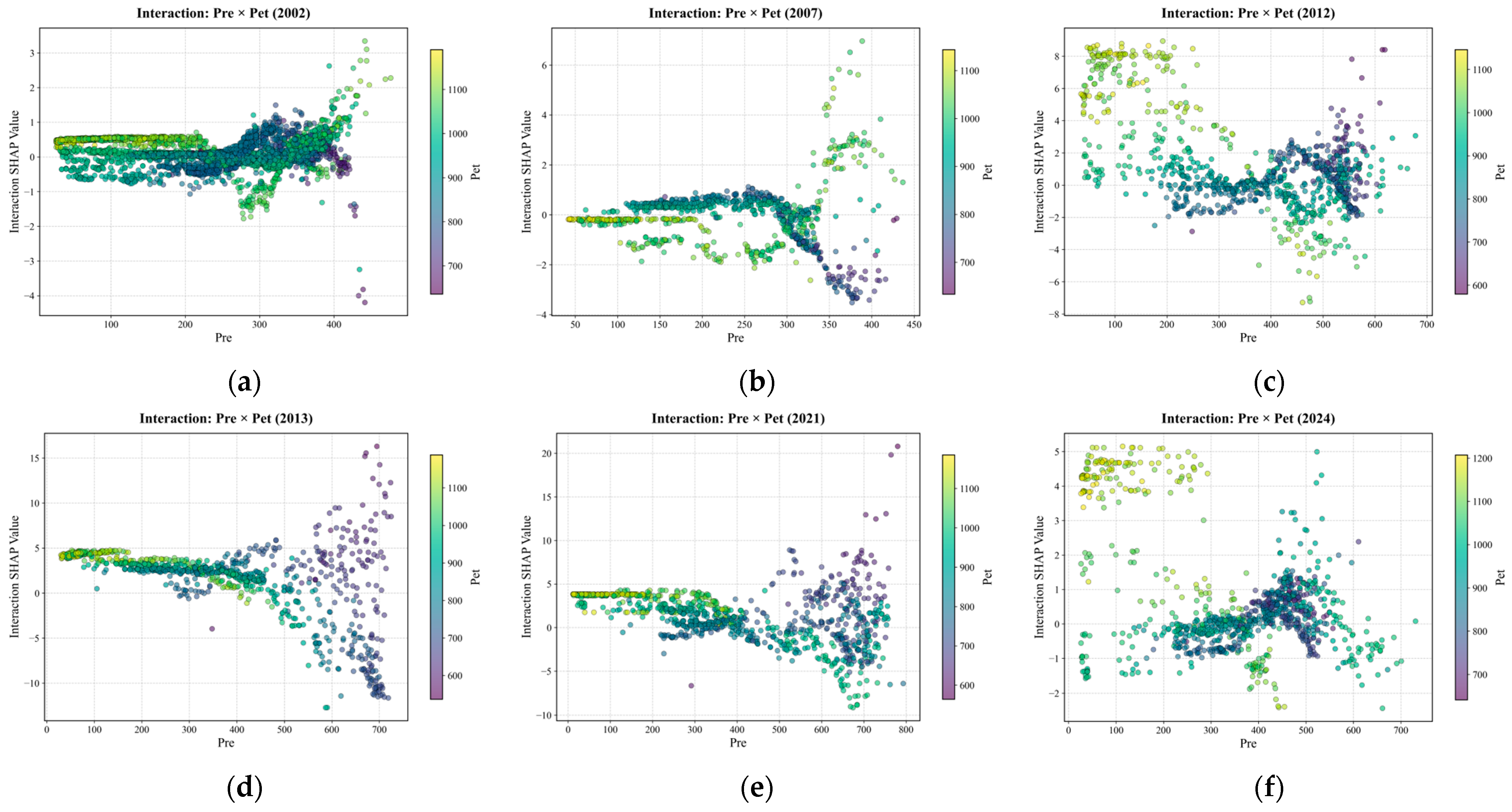
SHAP interactions between precipitation and evapotranspiration for the six characteristic years (Figure 16) can be summarized into three types of interannual response. The first type is weak modulation with high-rainfall crossover in dry years (2002, 2007): when precipitation is below ~300 mm, the joint contribution of precipitation and potential evapotranspiration is generally weak, and interaction values mostly lie near zero; after precipitation exceeds ~250–300 mm, high-Pet pixels mostly show an initial weakening followed by recovery as precipitation increases, whereas low-Pet pixels in the high-rainfall segment mostly show a near-zero or slightly negative downward trend. The second type is scissor-pattern divergence in wet years (2013, 2021): when precipitation is below ~400 mm, interaction effects across different Pet levels differ little and are mostly positive; after precipitation exceeds ~400–500 mm, interaction SHAP for high-Pet pixels continues to weaken with increasing precipitation and turns negative, whereas low-Pet pixels rise markedly in the high-rainfall segment. The third type is transitional or weakened (2012, 2024): in 2012, at low precipitation, interaction for high-Pet pixels remained mostly positive, and only after precipitation increased further did divergence emerge—high Pet negative and low Pet positive—with response directions in low- and high-rainfall segments opposite to the second type; in 2024, high-Pet pixels mainly shifted from positive to negative with increasing precipitation, whereas low-Pet pixels remained mostly near zero across the full precipitation range, and overall interaction strength was weaker than in 2013 and 2021.
Figure 16.
SHAP interaction of Pre and Pet. (a) 2002; (b) 2007; (c) 2012; (d) 2013; (e) 2021; (f) 2024.
4. Discussion
4.1. Geodetector Versus XGBoost–SHAP: Convergent Evidence and Methodological Differences
4.1.1. Factor Detection
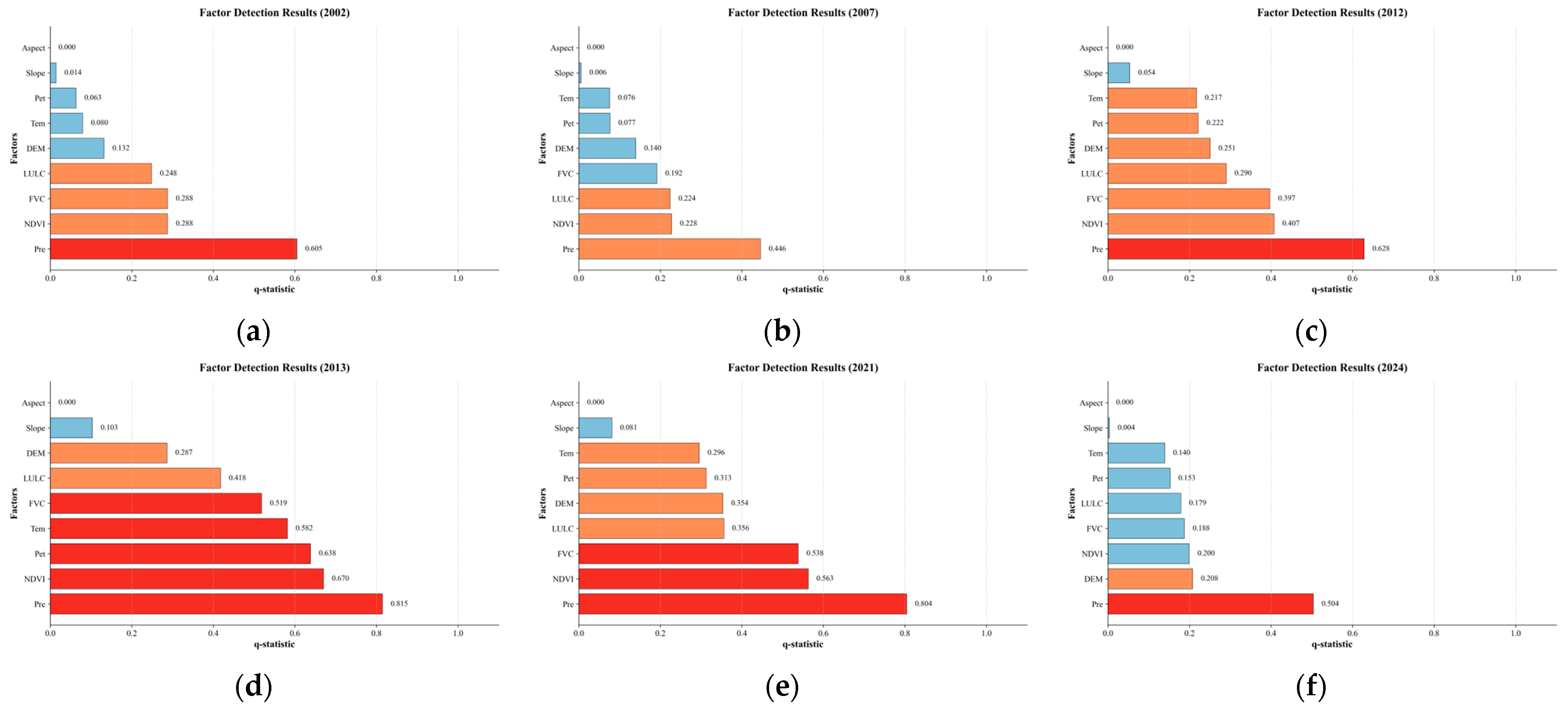
Geodetector q-value analysis results are shown in Figure 17. Both q values and mean |SHAP| indicate that precipitation is the primary factor, and Pre plays a stronger role in typical wet years than in dry years. The influence of NDVI and FVC on water yield differs between the two approaches: in wet years, q values for NDVI and FVC often rise to 0.4–0.7, second only to precipitation, which is inconsistent with the mid-to-lower rankings of NDVI and FVC in XGBoost–SHAP [15]. This is related to the fact that the geodetector measures whether vegetation indices and water yield are synchronously stratified in space, whereas SHAP explains the marginal contribution of NDVI and FVC to InVEST water-yield prediction after precipitation, land cover, and other factors are already included in the model. Rankings of q values and mean |SHAP| are broadly consistent for the remaining factors; the influence of slope and aspect is negligible, further supporting a mechanism of precipitation dominance coordinated with underlying surface and evapotranspiration background [12,37]. InVEST water-yield spatial differentiation studies in northwestern arid regions also support the view of joint precipitation–underlying-surface control [38].
Figure 17.
Factor-detection q charts. (a) 2002; (b) 2007; (c) 2012; (d) 2013; (e) 2021; (f) 2024.
4.1.2. Interaction Detection
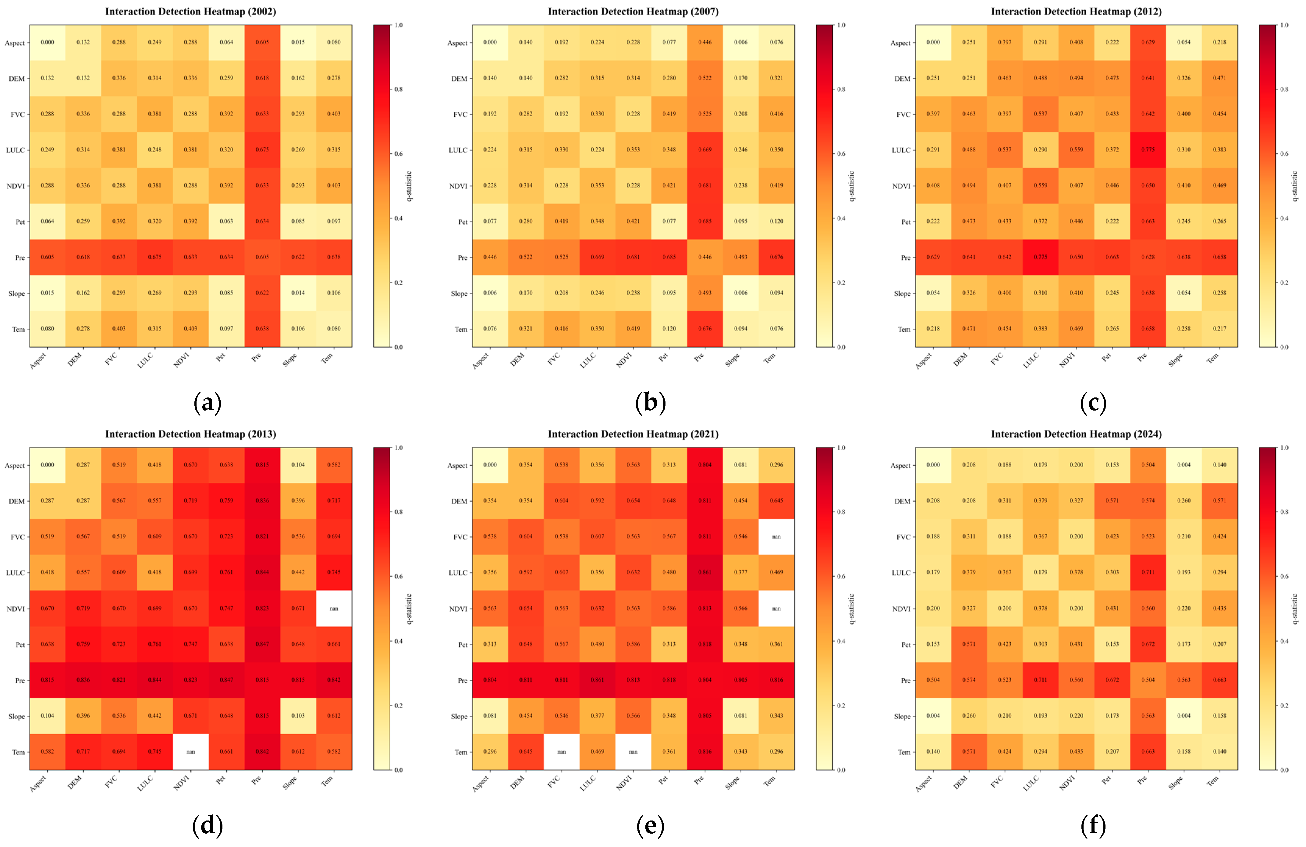
Geodetector interaction detection results (Figure 18) are generally consistent with SHAP interaction analysis in the overall pattern for the remaining factor pairs and year-specific interactions. Precipitation forms the highest-value “cross-shaped” core zone in the heatmap, and precipitation–land-use interaction intensity ranks among the highest across years, consistent with the precipitation–forest interaction results in SHAP. In individual years, especially 2007 and 2013, precipitation–potential evapotranspiration interaction is also prominent (~0.61–0.84), likewise corroborating the SHAP interaction results [34,37,39]. Interaction values for Tem × NDVI in 2013 and Tem × NDVI/FVC in 2021 are not shown (nan) because within-stratum variance could not be estimated after stratification, which does not affect the overall analysis.
Figure 18.
Interaction-detection charts. (a) 2002; (b) 2007; (c) 2012; (d) 2013; (e) 2021; (f) 2024.
4.1.3. Implications for XGBoost–SHAP Analysis
The geodetector corroborates XGBoost–SHAP results in terms of precipitation primacy, strengthened Pre effects in typical wet years, and prominent Pre × LULC and Pre × Pet interactions, indicating that the driver patterns revealed by SHAP are reliable at the level of spatial differentiation. Compared with the geodetector, SHAP further indicates whether factors promote or suppress water yield; the impact analysis can show when effects strengthen markedly after precipitation increases, as well as year-to-year differences in the combined effects of precipitation with forest land and evapotranspiration, offering finer interpretation that is closer to pixel-scale reality.
4.2. Mechanistic Interpretation of Spatial Heterogeneity in Water Yield
4.2.1. Spatial Patterns of Water Yield and Zonal Driver Heterogeneity
In terms of spatial heterogeneity of water-yield depth, the east-high/west-low pattern of water-yield depth is consistent with the spatial coupling of hydroclimate, geomorphic units, and vegetation belts among the southeastern monsoon margin, typical steppe, and inland arid zone. The East has relatively abundant precipitation and higher forest–grassland cover, with a multi-year mean water-yield depth of about 37 mm. The Central typical steppe zone has moderate precipitation and is mainly grassland, with a water-yield depth of about 7 mm. The western sandy land–Gobi zone is extremely arid, with a water-yield depth of only 0.03 mm, and effective precipitation is largely consumed by evapotranspiration [18,36]. “Precipitation dominance” also shows significant spatial differences. Although Pre is the highest-share factor in the East, Central, and West, the relative shares are 48.8%, 63.5%, and 37.7%, respectively, and secondary controls show east–west gradient reorganization: Forest (19.3%) and DEM (8.4%) are prominent in the East, barren land (7.0%) and Pet (5.9%) are secondary in the Central zone, and Pre and Tem have close relative shares in the West (37.7% and 32.1%), but |SHAP| magnitudes of all factors are very small. In terms of spatial heterogeneity of land use, in the eastern high-yield belt, the mean water-yield depths of forest, grassland, and cropland all increase with the precipitation gradient, but response magnitudes differ. In high-precipitation areas (>444 mm), mean water-yield depths are 101.8 mm for cropland, 81.1 mm for grassland, and 58.7 mm for forest, indicating that water-yield efficiency of different land-cover types in the East changes with the precipitation gradient. In terms of spatial heterogeneity of water-yield depth change, pixels with significant increases in water-yield depth are concentrated in the northeast and the southeastern foothills of the Greater Khingan Mountains, which may be related to ecological restoration projects and wetter background conditions [23]. The significant decrease belt in the south-central region may be related to cropland expansion and spatial differentiation of interannual precipitation variability [19,20]. The above trend interpretations are based on spatial overlap and are associational inferences.
4.2.2. Scale Dependence of Precipitation Dominance Under Uniform Z Calibration
In this study, the Z parameter was calibrated year by year (1.21–3.34) to match the regional total water yield reported in the bulletin, which is conducive to water-balance closure at the overall regional scale. However, Z was applied uniformly across the study area without considering differences in precipitation and water-yield levels among the East, Central, and West, so water-yield simulation accuracy was not consistent in the east–west direction. Mean test-set R2 values of zonal XGBoost were 0.875 in the East, 0.872 in the Central zone, and 0.843 in the West, and in 2024 the West was only 0.471. Mean water yield in the West was about 0.03 mm, and pixel-to-pixel differences were very small. Under such conditions, although Pre still ranked first in the SHAP results (about 37.7%), mean |SHAP| values of all factors were mostly around 0.02–0.03 mm, with very small absolute contributions, so interpretation of secondary factors needs to be treated with caution. In arid and semi-arid areas, how much water is yielded often depends first on effective precipitation, and differences in water yield among pixels also mainly change with precipitation, so precipitation usually ranks first in the SHAP results. This does not mean that land use has no effect; it is just that in low-yield areas such as the West, water-yield differences among forest, grassland, and cropland are relatively small, whereas in the East it is easier to see the effects of factors such as forest and topography. Because this study used regionally uniform Z-parameter calibration, the reliability of simulation and attribution results in the West is relatively weak; in the future, Z could be calibrated separately by subregion, or analysis could be conducted by partitioning according to high and low precipitation.
4.3. Limitations and Future Research
First, InVEST simplifies hydrological processes [40,41,42,43,44]. Although the Z parameter was adjusted year by year for 2001–2024 based on water resource bulletins to control regional total water yield, calibration still focused mainly on regional totals. In the absence of direct pixel-scale water-yield observations, this study compared InVEST-simulated AET outputs with GLEAM products for spatial validation as an indirect check. Watershed-scale assessments indicate that this approach has some feasibility in data-scarce regions [40,41], but it still cannot replace validation against gauged runoff [42]. Where pixel-scale water-yield observations are lacking, water-yield results often rely on mutual corroboration from multiple sources such as evapotranspiration products, bulletin totals, and spatial patterns [45], and judgments on the location of high-value patches should still be made with caution [1,35]. Because gauged runoff or independent water-yield observations could not be obtained, uncertainties from bulletin-based Z calibration (applied uniformly across subregions), input datasets, and indirect AET evaluation may affect the absolute magnitude and spatial pattern of simulated water yield, especially in the low-yield West, and these effects were not fully quantified in this study. The 2001–2024 period is shorter than the 30-year period commonly recommended for climatological representativeness. Therefore, this study does not aim to define a long-term climate normal, but rather to assess recent two-decade changes in water-yield depth under a consistent multi-source data framework. The period was selected because annual land-use, vegetation, climate, and water-resource bulletin data could be consistently matched during 2001–2024. The Sen–MK results should therefore be interpreted as recent-period trend characteristics rather than full climatological trends.
Second, XGBoost–SHAP and the geodetector parse driver relationships from the perspectives of model-prediction contribution and spatial differentiation, respectively. The two approaches corroborate each other regarding precipitation primacy and strengthened effects in typical wet years, but absolute SHAP values and q values have different meanings; the overall interpretation is associational and should not be directly equated with causal mechanisms [15].
Third, original data for precipitation, evapotranspiration, vegetation, land use, and topography differ in resolution; unified resampling, projection, and clipping alter within-pixel detail and may affect InVEST output accuracy. Biophysical parameters are assigned uniformly by land-cover type, which also involves regional differences given the strong east–west gradient in Inner Mongolia; the above errors may accumulate in simulation and attribution. These limitations have relatively limited impact on the main conclusion that “precipitation dominates, with land cover and evapotranspiration background modulating water yield.” Over longer time scales, the effects of climate change and land-use change on water yield have been widely discussed in other regions [46]. Future work will improve independent evapotranspiration and hydrological observation comparisons, refine data-processing schemes, and conduct sensitivity analysis of biophysical parameter tables.
The main findings apply most directly to Inner Mongolia and similar arid-to-semi-arid regions with strong hydroclimatic gradients. The integrated InVEST–Sen–MK–XGBoost–SHAP workflow can be transferred to other regions after local recalibration, but absolute water-yield values and driver rankings should not be directly extrapolated without re-simulation and independent validation. This study focused on locally generated water-yield depth simulated by the InVEST annual water yield module. Rivers, inter-basin water transfer, reservoir regulation, lake storage, and detailed water-management practices were not explicitly represented. Therefore, the east-high/west-low pattern should be interpreted as the spatial pattern of local water production rather than the final distribution of available water resources after hydrological regulation and human water management. Reservoirs and lakes may alter downstream water availability through storage and seasonal regulation, but these processes could not be quantified with the available data. Horizontal precipitation, such as fog and dew deposition, may also contribute to local water inputs in arid and semi-arid regions, especially in mountainous areas and forest margins. Because this study used gridded precipitation as the InVEST input, horizontal precipitation was not separately included. This may lead to slight underestimation of local water input in some eastern mountainous and forested pixels, although the effect on the regional total may be partly reduced by annual Z-parameter calibration against water-resource bulletin data.
5. Conclusions
This study conducted a regional integrated assessment of water-yield depth and its nonlinear drivers in Inner Mongolia within a unified spatial framework for 2001–2024. Based on year-by-year Z-parameter calibration against water resource bulletins, regional total water yield was broadly consistent with official statistics; however, because pixel-scale water-yield observations were unavailable, the GLEAM AET comparison was used only as an indirect check of the spatial plausibility of simulated water-yield depth and cannot replace direct validation of water-yield depth. Spatially, water-yield depth showed a marked east-high/west-low pattern, consistent with the east–west transition in hydroclimate and vegetation belts. Sen–MK trend analysis indicated that most pixels showed no significant change during the study period; significantly increasing areas were mainly concentrated in the relatively humid northeastern belt, whereas significantly decreasing areas were scattered in low-yield western zones.
Region-wide XGBoost–SHAP attribution showed that precipitation was the primary control on interannual and pixel-scale water-yield variation, with stronger effects in wet years and significant nonlinear modulation by land cover and evapotranspiration background. Comparisons among characteristic dry and wet years further indicated that mean |SHAP| values for precipitation were generally higher in wet years than in dry years, suggesting that driver structures were sensitive to interannual hydroclimatic backgrounds. Dependence analysis showed threshold-like precipitation responses that differed between dry and wet years: at low precipitation, SHAP values were mostly negative or near zero, whereas effects strengthened rapidly after precipitation exceeded certain levels, with inflection positions varying between dry and wet years. East–Central–West zonal models revealed spatially non-stationary driver structures: precipitation remained the highest-share factor in all three zones (48.8%, 63.5%, and 37.7% in the East, Central, and West, respectively), but secondary controls reorganized along the east–west gradient—forest and topography were dominant in the East, barren land and potential evapotranspiration were secondary in the Central steppe, and temperature had a relatively higher share under extremely low water yield in the West, where |SHAP| magnitudes of all factors were very small. These zonal results suggest that region-wide “precipitation dominance” should be interpreted together with local available water and attribution uncertainty, especially in the West. The geodetector corroborated SHAP results in factor detection and interaction detection, whereas SHAP further revealed directional effects of drivers and threshold-like nonlinear responses. Interaction analysis further indicated clear synergistic or antagonistic relationships between precipitation and forest land and between precipitation and potential evapotranspiration; under high precipitation, precipitation–non-forest land-cover interactions tended to diverge in a scissor-like pattern, whereas forest-related interactions remained relatively stable or turned negative, indicating that water-yield responses depended not only on single-factor strength but also on the combination of precipitation background and land-cover type.
Several limitations remain in this study. First, gauged runoff or independent water-yield observations were unavailable; bulletin-based calibration and indirect AET comparison were insufficient to fully verify pixel-scale water-yield magnitudes, and uniform Z-parameter calibration across subregions may introduce uncertainty in the extremely low-yield West. Second, the 2001–2024 series was shorter than the commonly used 30-year climatological reference period; trend results should therefore be interpreted as characteristics of change over the recent two decades rather than long-term climate-normal trends. Third, the InVEST Annual Water Yield module represents local water production and does not explicitly represent river flow, inter-basin water transfer, reservoir/lake regulation, or horizontal precipitation; these issues were discussed but were not incorporated into quantitative modeling. Fourth, uncertainty sources related to input resampling, resolution differences, and biophysical parameter assignment were not fully quantified, and their effects on absolute magnitudes may exceed those on the main qualitative spatial patterns.
Author Contributions
Conceptualization, C.F. and T.W.; methodology, C.F., X.L. and T.W.; software, C.F.; validation, T.W. and X.L.; formal analysis, C.F., B.Z. and D.L.; investigation, C.F. and B.Z.; resources, X.L.; data curation, C.F.; writing—original draft preparation, C.F.; writing—review and editing, T.W., X.L., B.Z. and D.L.; visualization, C.F. and D.L.; supervision, T.W. and X.L.; project administration, T.W.; funding acquisition, T.W. All authors have read and agreed to the published version of the manuscript.
Funding
This research was funded by the Inner Mongolia Autonomous Region Key Research and Development and Achievement Transformation Program, grant number 2026YFHH0082; the Natural Science Foundation of Inner Mongolia Autonomous Region, grant numbers 2024MS05053, 2024QN04023, 2025QN03134 and 2026LHMS0099; the Inner Mongolia Postdoctoral Research Funding Program for Postdoctoral Researchers Remaining in Inner Mongolia, grant number nmgbshjf2501; and the Doctoral Research Fund of Jining Normal University, grant numbers jsbsjj2324 and jsbsjj1802.
Data Availability Statement
The original contributions presented in this study are included in the article material. Further inquiries can be directed to the corresponding author(s).
Acknowledgments
We thank the Inner Mongolia Autonomous Region Water Resources Bulletin for providing hydrological statistics, and the institutions maintaining and distributing the open-access datasets used in this study.
Conflicts of Interest
The authors declare no conflicts of interest. The funders had no role in the design of the study; in the collection, analyses, or interpretation of data; in the writing of the manuscript; or in the decision to publish the results.
References
- Mukhopadhyay, A.; Hati, J.P.; Acharyya, R.; Pal, I.; Tuladhar, N.; Habel, M. Global trends in using the InVEST model suite and related research: A systematic review. Ecohydrol. Hydrobiol. 2025, 25, 389–405. [Google Scholar] [CrossRef] [Scilit]
- Qiao, Y.J.; Zhang, H.; Han, X.Y.; Liu, Q.B.; Liu, K.; Hu, M.T.; Pei, W.M. Exploring Drivers of Water Conservation Function Variation in Heilongjiang Province from a Geospatial Perspective. Acta Ecol. Sin. 2023, 43, 2711–2721. [Google Scholar] [CrossRef] [Scilit]
- Lü, M.X.; Zhang, H.; He, G.Z.; Zhang, X.Y.; Liu, Y. Dynamic Evolution and Driving Factors of Water Conservation Service Function in the Yellow River Basin. Acta Ecol. Sin. 2024, 44, 2761–2771. [Google Scholar] [CrossRef]
- Hu, J.; Wang, L.; Wang, Y.; Liu, Y.; Su, X.; Li, L.; Li, J. Driving Mechanisms of Water Yield in the Yellow River Basin: Insights from an Explainable Machine Learning Approach. J. Hydrol. Reg. Stud. 2025, 61, 102610. [Google Scholar] [CrossRef] [Scilit]
- Li, H.; Zhang, Y.; Wang, J.; Li, Y.; Zhang, X. Evolution and Analysis of Water Yield under the Change of Land Use and Climate Change Based on the PLUS-InVEST Model: A Case Study of the Yellow River Basin in Henan Province. Water 2024, 16, 2551. [Google Scholar] [CrossRef] [Scilit]
- Zhang, X.J.; Long, Y.H.; Liao, Z.L.; Suo, M.Q. Temporal and Spatial Variation of Water Yield in the Tabu River Basin of the Northern Yinshan Mountain. J. Irrig. Drain. 2023, 42, 98–107. [Google Scholar] [CrossRef]
- An, N.; Li, H.; Bai, Y. Spatial-Temporal Characteristics and Driving Forces of Water Yield in the Qinghai-Tibet Plateau Based on the InVEST Model and Geodetector. Sustainability 2022, 14, 12389. [Google Scholar] [CrossRef] [Scilit]
- Feng, H.; Zhao, W.; Li, A.; Zhang, F. Spatiotemporal Variation of Water Yield and Its Driving Forces in the Middle Reaches of the Heihe River Basin Based on InVEST. Water 2020, 12, 3103. [Google Scholar] [CrossRef] [Scilit]
- Lee, S.-I. Developing a Bivariate Spatial Association Measure: An Integration of Pearson’s r and Moran’s I. J. Geogr. Syst. 2001, 3, 369–385. [Google Scholar] [CrossRef] [Scilit]
- Sen, P.K. Estimates of the Regression Coefficient Based on Kendall’s Tau. J. Am. Stat. Assoc. 1968, 63, 1379–1389. [Google Scholar]
- Mann, H.B. Nonparametric Tests against Trend. Econom. J. Econom. Soc. 1945, 13, 245–259. [Google Scholar] [CrossRef] [Scilit]
- Wang, J.F.; Xu, C.D. Geodetector: Principle and Prospective. Acta Geogr. Sin. 2017, 72, 116–134. [Google Scholar] [CrossRef]
- Chen, T.; Guestrin, C. XGBoost: A Scalable Tree Boosting System. In Proceedings of the 22nd ACM SIGKDD International Conference on Knowledge Discovery and Data Mining, San Francisco, CA, USA, 13–17 August 2016; pp. 785–794. [Google Scholar]
- Lundberg, S.M.; Lee, S.-I. A Unified Approach to Interpreting Model Predictions. In Advances in Neural Information Processing Systems 30; Curran Associates, Inc.: Red Hook, NY, USA, 2017; pp. 4765–4774. [Google Scholar]
- Slater, L.J.; Blougouras, G.; Deng, L.; Deng, Q.; Ford, E.; Hoek van Dijke, A.; Huang, F.; Jiang, S.; Liu, Y.; Moulds, S.; et al. Challenges and Opportunities of ML and Explainable AI in Large-Sample Hydrology. Phil. Trans. R. Soc. A 2025, 383, 20240287. [Google Scholar] [CrossRef] [Scilit] [PubMed]
- Li, H.; Chen, Y.; Zhang, K.; Wang, J.; Liu, X. Revealing Nonlinear Relationships and Thresholds of Human Activities and Climate Change on Ecosystem Services in Anhui Province Based on the XGBoost–SHAP Model. Sustainability 2025, 17, 8728. [Google Scholar] [CrossRef] [Scilit]
- Huang, Y.; Wang, D.C.; Ouyang, H.L.; Han, J.X.; Zhuang, C.Y. Identification of Driving Factors for Water Supply Service in Sichuan Province, Southwest China from a Machine Learning Perspective. Chin. J. Appl. Ecol. 2025, 36, 2171–2182. [Google Scholar] [CrossRef] [Scilit] [PubMed]
- Zhou, A.F.; Zhao, W.W.; Pereira, P. Mapping and Assessing Freshwater Ecosystem Services Supply and Demand in Inner Mongolia (China). Landsc. Ecol. 2023, 38, 1885–1902. [Google Scholar] [CrossRef] [Scilit]
- Hao, L.; Wang, S.; Cui, X.P.; Lei, H.G. Quantitative Assessment of Climate Change, Land Conversion, and Management Measures on Key Ecosystem Services in Arid and Semi-Arid Regions: A Case Study of Inner Mongolia, China. Sustainability 2025, 17, 6348. [Google Scholar] [CrossRef] [Scilit]
- Gong, J.; Shi, J.; Zhu, C.; Li, X.; Zhang, Z.; Zhang, W.; Li, Y.; Hu, Y. Accounting for Land Use in an Analysis of the Spatial and Temporal Characteristics of Ecosystem Services Supply and Demand in a Desert-Oasis City of Inner Mongolia, China. Ecol. Indic. 2022, 142, 109246. [Google Scholar] [CrossRef] [Scilit]
- Inner Mongolia Autonomous Region Water Resources Department. Inner Mongolia Water Resources Bulletin, Hohhot, China, 2021–2024. Available online: https://slt.nmg.gov.cn/ (accessed on 6 June 2026).
- Li, H.Y.; Ma, L.; Liu, T.X.; Du, Y.X.; Liu, M. Change and Relationship of Temperature and Precipitation in Inner Mongolia during 1951–2014. J. Glaciol. Geocryol. 2017, 39, 1098–1112. [Google Scholar] [CrossRef]
- Kui, G.X.; Shi, C.Q.; Yang, J.Y.; Li, R.P.; Wei, G.K.; Liu, J.Q. Spatial-Temporal Variations of Vegetation Coverage and Its Driving Force in Inner Mongolia Grassland, China. Chin. J. Appl. Ecol. 2023, 34, 2713–2722. [Google Scholar] [CrossRef] [Scilit] [PubMed]
- Natural Capital Project. InVEST 3.12.0 User’s Guide; Stanford University: Stanford, CA, USA, 2020; Available online: https://naturalcapitalproject.stanford.edu/software/invest (accessed on 6 June 2026).
- Martens, B.; Miralles, D.G.; Lievens, H.; van der Schalie, R.; de Jeu, R.A.M.; Fernández-Prieto, D.; Beck, H.E.; Dorigo, W.A.; Verhoest, N.E.C. GLEAM v3: Satellite-Based Land Evaporation and Root-Zone Soil Moisture. Geosci. Model Dev. 2017, 10, 1903–1925. [Google Scholar] [CrossRef] [Scilit]
- Miralles, D.G.; Holmes, T.R.H.; De Jeu, R.A.M.; Gash, J.H.; Meesters, A.G.C.A.; Dolman, A.J. Global Land-Surface Evaporation Estimated from Satellite-Based Observations. Hydrol. Earth Syst. Sci. 2011, 15, 453–469. [Google Scholar] [CrossRef] [Scilit]
- Peng, S.Z.; Ding, Y.X.; Liu, W.Z.; Li, Z. The 1 km Monthly Temperature and Precipitation Dataset for China from 1901 to 2017. Earth Syst. Sci. Data 2019, 11, 1931–1946. [Google Scholar] [CrossRef] [Scilit]
- Yang, J.; Huang, X. The 30 m Annual Land Cover Dataset and Its Dynamics in China from 1990 to 2019. Earth Syst. Sci. Data 2021, 13, 3907–3925. [Google Scholar] [CrossRef] [Scilit]
- Peng, S.Z. 1-km Monthly Potential Evapotranspiration Dataset for China (1901–2023); National Tibetan Plateau/Third Pole Environment Data Center: Beijing, China, 2022. [Google Scholar] [CrossRef]
- FAO/IIASA/ISRIC/ISS-CAS/JRC. Harmonized World Soil Database (version 1.2); FAO: Rome, Italy; IIASA: Laxenburg, Austria, 2012; Available online: https://www.fao.org/soils-portal/data-hub/soil-maps-and-databases/harmonized-world-soil-database-v12/en/ (accessed on 6 June 2026).
- Yan, F.P.; Shangguan, W.; Zhang, J.; Hu, B.F. Depth-to-Bedrock Map of China at a Spatial Resolution of 100 Meters. Sci. Data 2020, 7, 2. [Google Scholar] [CrossRef] [Scilit] [PubMed]
- Wu, C.X.; Qiu, D.X.; Gao, P.; Mu, X.M.; Zhao, G.J. Application of the InVEST Model for Assessing Water Yield and Its Response to Precipitation and Land Use in the Weihe River Basin, China. J. Arid Land 2022, 14, 426–440. [Google Scholar] [CrossRef] [Scilit]
- Yin, G.D.; Wang, X.; Zhang, X.; Fu, Y.; Hao, F.; Hu, Q. InVEST Model-Based Estimation of Water Yield in North China and Its Sensitivities to Climate Variables. Water 2020, 12, 1692. [Google Scholar] [CrossRef] [Scilit]
- Wang, J.F.; Li, X.H.; Christakos, G.; Liao, Y.L.; Zhang, T.; Gu, X.; Zheng, X.Y. Geographical Detectors-Based Health Risk Assessment and Its Application in the Neural Tube Defects Study of the Heshun Region, China. Int. J. Geogr. Inf. Sci. 2010, 24, 107–127. [Google Scholar] [CrossRef] [Scilit]
- Wang, B.; Zhu, G.F.; Zhong, J.T.; Ma, C.F.; Zhang, L.; Tan, M.B.; Li, X. Uncertainty Analysis and Parameter Optimization of a Water Yield Ecosystem Service Model: A Case Study of the Qilian Mountains, China. Sci. Total Environ. 2025, 966, 178772. [Google Scholar] [CrossRef] [Scilit] [PubMed]
- Dou, H.S.; Li, X.B.; Li, S.K.; Dang, D.; Li, X.; Lyu, X.; Li, M.; Liu, S. Mapping Ecosystem Services Bundles for Analyzing Spatial Trade-Offs in Inner Mongolia, China. J. Clean. Prod. 2020, 256, 120444. [Google Scholar] [CrossRef] [Scilit]
- Li, T.; Wang, W.; Zhang, D.; Chen, Y.; Li, H. Evaluate Water Yield and Soil Conservation and Their Environmental Gradient Effects in Fujian Province in South China Based on InVEST and Geodetector Models. Water 2024, 17, 230. [Google Scholar] [CrossRef] [Scilit]
- Li, F.; Li, Y.M.; Zhou, X.W.; Yin, Z.; Liu, T.; Xin, Q.C. Modeling and Analyzing Supply–Demand Relationships of Water Resources in Xinjiang from a Perspective of Ecosystem Services. J. Arid Land 2022, 14, 115–138. [Google Scholar] [CrossRef] [Scilit]
- Yang, S.C.; Li, H.R.; Yang, S.; Li, Y. Spatiotemporal Evolution of Water Yield Services and Multiscale Driving Effects in an Arid Watershed: A Case Study of the Aksu River Basin. Sustainability 2022, 14, 818. [Google Scholar]
- Hamel, P.; Bryant, B.P. Uncertainty Assessment in Ecosystem Services Analyses: Seven Challenges and Practical Responses. Ecosyst. Serv. 2017, 24, 1–15. [Google Scholar] [CrossRef] [Scilit]
- Redhead, J.W.; Stratford, C.; Sharps, K.; Jones, L.; Ziv, G.; Clarke, D.; Oliver, T.H.; Bullock, J.M. Empirical Validation of the InVEST Water Yield Ecosystem Service Model at a National Scale. Sci. Total Environ. 2016, 569–570, 1418–1426. [Google Scholar] [CrossRef] [Scilit] [PubMed]
- Redhead, J.W.; May, L.; Oliver, T.H.; Hamel, P.; Sharp, R.; Bullock, J.M. National Scale Evaluation of the InVEST Model for a High Quality National Scale Validation Process. Ecosyst. Serv. 2020, 46, 101209. [Google Scholar]
- Valencia, J.B.; Mesa-Díez, J.; Valencia-Romero, J.; Tapasco, J.; Gusarov, A.V. Assessing the Effectiveness of the Use of the InVEST Annual Water Yield Model for the Rivers of Colombia: A Case Study of the Meta River Basin. Water 2023, 15, 1617. [Google Scholar] [CrossRef] [Scilit]
- Valencia-García, J.B.; Guryanov, V.V.; Mesa-Díez, J.; Tapasco, J.; Gusarov, A.V. Predictive Assessment of Climate Change Impact on Water Yield in the Meta River Basin, Colombia: An InVEST Model Application. Hydrology 2024, 11, 25. [Google Scholar] [CrossRef] [Scilit]
- Huang, L.; Lyu, Y.; Miao, L.; Li, S. Balancing Hydrological Sustainability and Heritage Conservation: A Decadal Analysis of Water-Yield Dynamics in the Honghe Hani Rice Terraces. Hydrology 2025, 12, 135. [Google Scholar] [CrossRef] [Scilit]
- Zhiña, D.X.; Avilés, A.; González, L.; Astudillo, A.; Astudillo, J.; Matovelle, C. Effects of Climate Change and Changes in Land Use and Cover on Water Yield in an Equatorial Andean Basin. Hydrology 2024, 11, 157. [Google Scholar] [CrossRef] [Scilit]

Disclaimer/Publisher’s Note: The statements, opinions and data contained in all publications are solely those of the individual author(s) and contributor(s) and not of MDPI and/or the editor(s). MDPI and/or the editor(s) disclaim responsibility for any injury to people or property resulting from any ideas, methods, instructions or products referred to in the content. |
© 2026 by the authors. Licensee MDPI, Basel, Switzerland. This article is an open access article distributed under the terms and conditions of the Creative Commons Attribution (CC BY) license.