Distributed Estimation of the Curve Number (CN) in Continental Ecuador Using Machine Learning, Official Geo-Pedological Data, and Field-Based Hydrological Validation

Abstract

The Curve Number (CN) remains one of the most widely applied parameters for estimating direct surface runoff. However, its conventional application based on watershed-aggregated tabulated values conceals hydrological variability in regions with contrasting soils and steep topographic gradients. A recurring limitation of distributed CN approaches is the absence of independent hydrological validation; most machine learning models are trained and evaluated against the same SCS-USDA lookup values used to construct the training target, a circular scheme that measures statistical agreement rather than physical credibility. This study develops a reproducible geospatial workflow for distributed CN estimation across continental Ecuador, combining official MAG land use, soil surface texture natural drainage, and topographic slope layers at 1:25,000 scale with a Random Forest regression model at 10 m spatial resolution. The CN reference raster was derived from official geo-pedological layers and independently validated, not against tabulated assumptions, but against observed hydrological behaviour. Field hydraulic characterization across four dominant land cover classes in the Guamote microwatershed (Chimborazo Province), combined with HEC-HMS (US Army Corps of Engineers, Davis, CA, USA) rainfall-runoff modelling over 41 years (1981–2021), confirmed a mean annual discharge of 0.1568 m³ s⁻¹ consistent with the tabulated CN assignments. To our knowledge, this is the first nationally distributed CN map with field-anchored hydrological benchmarking for an Andean country. The Random Forest model achieved an RMSE = 10.4, an R² = 0.42, and an NSE = 0.41, a performance consistent with published field-based CN estimation studies and expected given the inherent scatter of the SCS-USDA method under real-world conditions. Zonal CN comparisons confirmed a mean absolute error below 5 CN units across the Andean highland and Amazon watersheds; the Guamote watershed showed a mean ∆CN below 4 units against the field-calibrated model. Land use and surface texture emerged as the dominant CN predictors, with natural drainage providing critical discrimination in volcanic and poorly drained soil environments. The resulting 10 m national CN map offers a physically grounded, spatially explicit parameterization layer for distributed hydrological modeling and water resources planning across data-scarce Andean and tropical territories, with direct relevance for flood risk screening, irrigation planning, watershed conservation, and climate adaptation under SDG 6, SDG 11, SDG 13 and SDG 15.

1. Introduction

The Curve Number (CN), developed by the Soil Conservation Service (SCS) of the United States Department of Agriculture (USDA), remains one of the most widely applied methods for estimating direct surface runoff from precipitation events [1,2,3,4,5]. Its conceptual simplicity, modest data requirements, and compatibility with operational hydrology models such as HEC-HMS and SWAT [6,7,8] have driven its adoption across a broad range of water resource management, land use planning, and flood risk assessment applications worldwide. In territories characterized by strong altitudinal gradients, contrasting soil orders, and rapidly varying land cover, such as the Andean region of Ecuador, the spatial representation of CN is particularly consequential, as small errors in runoff potential at the pixel scale propagate into significant uncertainties in watershed-scale water balance and flood frequency estimates.

The CN method, however, carries well-documented limitations when applied beyond the environmental conditions for which its lookup tables were originally calibrated [3,9,10]. The SCS tables were constructed under specific climatic and edaphic conditions prevailing in the continental United States; their direct application worldwide introduces structural uncertainties related to differences in soil genesis, vegetation phenology, and antecedent moisture dynamics [11,12]. In Andean countries such as Ecuador, where steep altitudinal gradients, diverse soil taxonomy, and highly variable land cover coexist within small spatial extents, the assignment of a single aggregated CN value per watershed suppresses the intra-catchment hydrological variability that controls local runoff generation and peak flow timing [13,14].

Machine learning techniques, combined with high-resolution geospatial data, have emerged as a promising alternative for improving the spatial representation of CN [15]. Algorithms such as Random Forest, Artificial Neural Networks, and gradient boosting methods have demonstrated the ability to capture non-linear relationships among edaphic, topographic, and land cover variables, yielding spatially explicit CN estimates at scales not accessible through conventional tabulation [15,16,17,18,19]. Despite this progress, most published applications remain confined to local or experimental catchments, and systematic national-scale implementations are notably absent from Latin American literature [20]. Furthermore, the methodological transferability of these approaches to a data-scarce Andean setting, where neither continuous discharge records nor high-resolution soil surveys are routinely available, has not been systematically evaluated.

A recurring and structurally important limitation of existing distributed CN studies is the absence of independent hydrological validation [21,22]. Most machine learning models are trained and evaluated against CN values derived exclusively from SCS-USDA lookup tables, producing circular validation schemes in which model performance is measured against the very assumptions embedded in the training data. This limitation is compounded in regions such as Ecuador, where the scarcity of continuous rainfall-runoff records restricts the possibility of calibrating CN values against observed discharge, making a physically grounded training reference particularly difficult to establish [11,23].

The release of official geo-pedological information at 1:25,000 scale by the Ministry of Agriculture and Livestock of Ecuador (MAG) represents a significant opportunity to advance distributed CN estimation in the region. These datasets integrate soil surface texture, natural drainage class, and land use at national coverage, providing a physically consistent basis for spatially explicit CN derivation consistent with SCS-USDA criteria. Despite this potential, their combined application with machine learning and field-based hydrological validation has not previously been reported in the literature for national-scale CN mapping [17,18,19].

Against this background, the present study develops a reproducible geospatial workflow for distributed CN estimation across continental Ecuador. Official land use, soil texture, natural drainage, and topographic slope layers at 1:25,000 scale are combined with a Random Forest regression model at 10 m resolution, trained on a CN reference raster grounded in both SCS-USDA tabulated criteria and independent field-based hydrological validation. Four objectives guide the work: producing a continuous CN map at 10 m resolution for continental Ecuador; quantifying model performance against a nationally distributed CN map with field-anchored hydrological benchmarking; evaluating spatial consistency through zonal CN comparisons at watershed scale and analyzing variable importance at national and regional scales. By strengthening spatial decision support for watershed planning and risk-informed land management, the workflow contributes to SDG 6, SDG 11, SDG 13, and SDG 15.

2. Materials and Methods

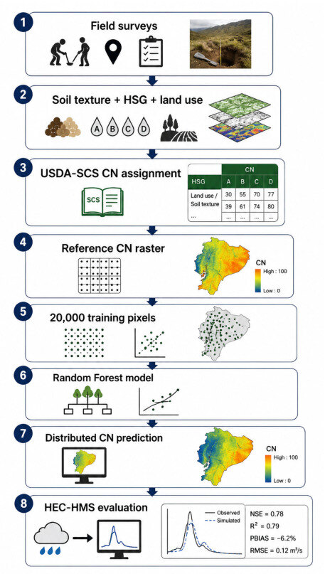
The methodological framework developed in this study integrates four components: (i) the compilation and harmonization of official geospatial layers representing the primary physical controls of surface runoff generation, (ii) the construction of a spatially distributed CN reference raster grounded in SCS-USDA tabulated criteria and hydrologically benchmarked through independent field validation, (iii) the training and spatial application of a Random Forest regression model at 10 m resolution, and (iv) a two-tier model benchmarked through combining pixel-level statistical metrics with watershed-scale zonal comparison. Figure 1 provides a schematic overview of the full workflow. The following subsections describe each component in detail.

Figure 1. Methodological workflow for distributed CN estimation across continental Ecuador, integrating official geo-pedological data, GIS preprocessing, and Random Forest modeling.

2.1. Study Area

The study covers continental Ecuador, encompassing approximately 256,370 Km² (90% of national territory); the Galapagos archipelago was excluded due to its geographic discontinuity and distinct pedological regime. Because continental Ecuador spans UTM Zones 17S and 18S, a single UTM projection would introduce unacceptable metric distortion at the national scale. All geospatial processing was therefore performed in a Lambert Conformal Conic projection parameterized for Ecuador (standard parallels and central meridian set to national extent), which preserves area and shape consistency across the entire territory and is appropriate for the zonal area-based statistics used in this study. Field-scale data for the Guamote microwatershed, which lies entirely within Zone 17S, were processed and are reported in UTM WGS84 Zone 17S.

Ecuador comprises three major physiographic regions (Coast, Andean Highlands and Amazon) that differ markedly in geology, soil formation processes, land use patterns, and precipitation regimes. The altitudinal range spans from sea level to over 6263 m a.s.l. (Chimborazo volcano) generating steep environmental gradients over short horizontal distances and producing some of the highest levels of edaphic and land cover heterogeneity found in any comparably sized territory. Mean annual precipitation ranges from below 500 mm yr⁻¹ in inter-Andean dry valleys to over 3000 mm yr⁻¹ in windward Amazonian slopes, directly conditioning infiltration capacity, runoff generation mechanisms, and CN spatial variability. These physiographic contrasts make Ecuador an ideal and methodologically demanding context for national-scale distributed CN mapping.

Field-based hydrological validation was conducted in the Guamote microwatershed (Chimborazo Province, 2° 56′ S, 78°42′ W), a paramo-agricultural system representative of the dominant land cover mosaic and soil orders of the Ecuadorian highlands. The watershed drains an area of approximately 567.67 Km² and exhibits altitudinal ranges and land use transitions characteristic of inter-Andean basins across the regions.

2.2. Geospatial Data Sources

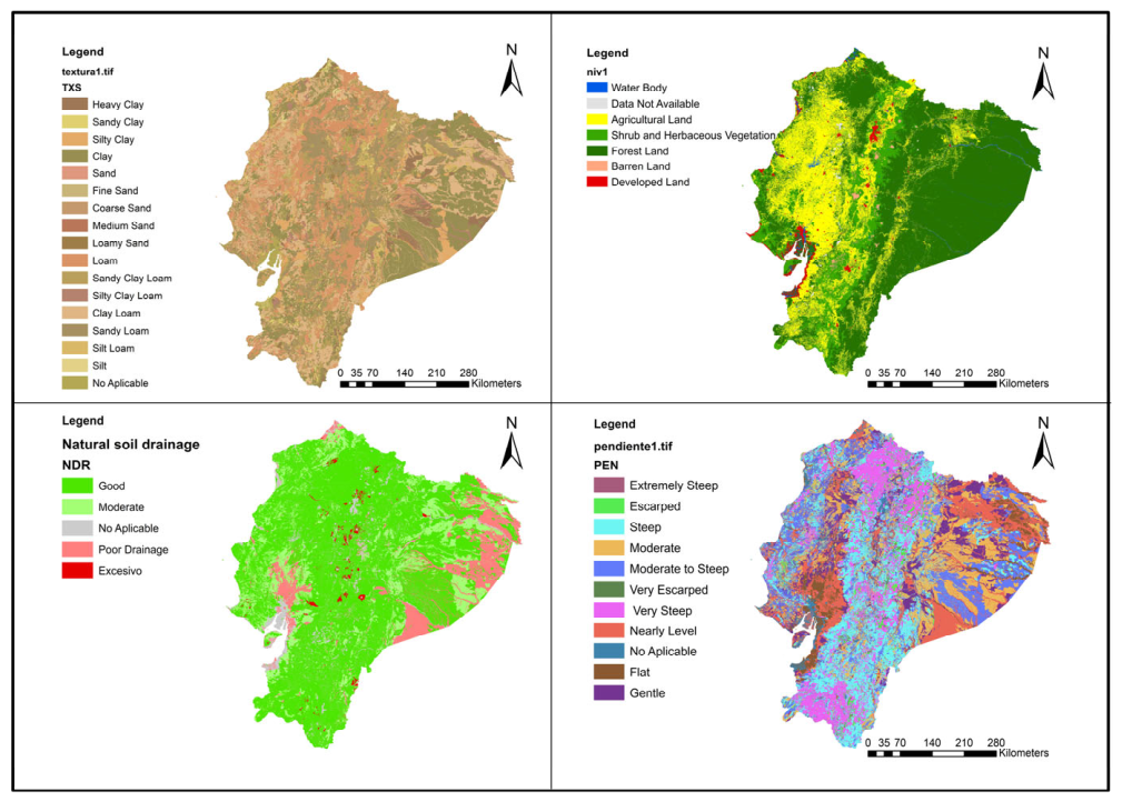
Official national geospatial datasets at a nominal scale of 1:25,000 were used to represent the primary controls of the SCS Curve Number framework (Table 1, Figure 2). Land use data were obtained from Level II Land Cover and Use Classification (CUT II, acquisition year 2016–2018) produced by the Ministry of Agriculture and Livestock (MAG). Soil surface texture and natural drainage were extracted from the Geo-pedological Map of Ecuador [24] (MAG survey period 2009–2015), which integrates edaphic and geomorphological information at national coverage. Elevation data were obtained from the ALOS World 3D–30 m Digital Surface Model (AW3D30), developed by the Japan Aerospace Exploration Agency (JAXA, Tokyo, Japan) [25]. The dataset provides near-global elevation coverage derived from the Panchromatic Remote-sensing Instrument for Stereo Mapping (PRISM) onboard the Advanced Land Observing Satellite (ALOS) mission, after we reclassified it into five percent-slope intervals following standard SCS-CN adjustment thresholds: 0–3%, 3–8%, 8–15%, 15–30% and >30%. Watershed boundaries for zonal validation were obtained from the Level III Pfafstetter watershed classification produced by the Ministry of Environment (MAE). All predictor layers were converted to raster format and harmonized to a common 10 m grid prior to modeling.

Table 1. Geospatial datasets.

Dataset	Source	Spatial Resolution/Scale	Description
Land use (CUT II)	Ministry of Agriculture and Livestock (MAG)	1:25,000	Land cover and land use classification used to assign CN values based on SCS–USDA tables.
Soil surface texture	Geo-pedological Map (MAG)	1:25,000	Used to determine Hydrologic Soil Group (HSG)
Natural drainage	Geo-pedological Map (MAG)	1:25,000	Refines Hydrologic Soil Group classification
Digital Elevation Model	ALOS World 3D–30 m Digital Surface Model	10 m	Used to derive slope values
Watershed boundaries	Level III Pfafstetter (MAE)	1:25,000	Spatial analysis and zonal validation

Figure 2. Spatial distribution of the predictor layers used in the Random Forest CN model across continental Ecuador, including natural soil drainage, land use and land cover (CUT II), topographic slope, and soil surface texture. Classification intervals and source metadata are detailed in Table 1. The full land use–soil texture–HSG–CN correspondence table is provided as Supplementary Material (Table S1).

2.3. GIS Preprocessing

All geospatial processing was performed in the R statistical environment (RStudio 2026.01.2) using the terra package as the primary geographic engine (R Foundation for Statistical Computing, Vienna, Austria). All layers for national-scale processing were reprojected to the Lambert Conformal Conic projection parameterized for Ecuador (consistent with Section 2.1) to ensure metric consistency across UTM Zones 17S and 18S and clipped to the national boundary extent using official Level III Pfafstetter watershed polygons. Field-scale data for the Guamote microwatershed, which lies entirely within Zone 17S, were processed in UTM WGS84 Zone 17S. Cells with null, inconsistent, or physically implausible values (CN < 0 or CN > 100) were masked and excluded from subsequent analysis. Categorical predictor variables (land use, soil texture, natural drainage) were resampled to the 10 m target grid using nearest-neighbor interpolation to preserve class integrity; the continuous slope variable was resampled using bilinear interpolation. The final harmonized raster stack covered approximately 2.56 × 10⁹ pixels at 10 m resolution. To manage this computational demand, national processing was implemented using tiled parallel execution via the terra parallel.

2.4. Construction and Hydrological Benchmarking of the Reference CN Raster

The CN reference raster used for model training was constructed through a two-stage process: (i) national spatial implementation of the SCS-USDA tabulated CN method applied to official MAG land use and soil property layers, and (ii) independent hydrological anchoring of the resulting raster through field-based validation in the Guamote microwatershed.

The objective of the field campaign was not to generate a fully field-derived national CN map, which would be impractical at continental scale, but rather to physically and hydrologically benchmark the tabulated SCS-USDA CN assignments under representative Andean conditions. The validated raster therefore served as a physically consistent reference dataset for subsequent Random Forest training and spatial generalization.

The Random Forest model was used as a spatial generalization framework to predict distributed CN values continuously across continental Ecuador at 10 m resolution while preserving the physical relationships embedded in the hydrologically benchmarked reference CN raster. Each pixel of the national raster was assigned a CN value by cross-referencing the land use class (CUT II), surface texture-derived Hydrologic Soil Group (HSG), and slope class following standard SCS-USDA lookup tables [1,3,5]. Soil texture classes were translated into HSG categories (A through D) according to NRCS criteria, with natural drainage used to refine HSG assignment in texture classes with ambiguous drainage characteristics (e.g., sandy clay loam with impeded natural drainage reclassified from HSG B to HSG C).

2.5. Field-Based Hydrological Anchoring

The physical consistency of the tabulated CN assignment was validated through systematic in situ hydraulic characterization conducted across four dominant land cover classes in the Guamote microwatershed: cultivated land, shrub vegetation, paramo, and forest plantations. Field sampling involved the extraction of soil cores at four depth intervals (0–20, 20–40, 40–60 and 60–80 cm) at 17 sampling sites stratified by land cover class and soil taxonomic unit. Laboratory analyses determined soil texture using the USDA particle size triangle method, porosity from apparent and real bulk density measurements, organic matter content by loss on ignition at 550 °C, and saturated hydraulic conductivity using a constant head permeameter following Darcy’s Law. Steady-state infiltration rates were measured at each sampling site using a custom-built double-ring infiltrometer following ASTM procedures. The hydraulic parameters derived from field and laboratory analyses were used to assign HSG categories consistent with NRCS criteria, which were then compared against the tabulated HSG assignments to confirm or correct CN values at each validation site.

In the absence of streamflow gauging stations (ungauged basin), model consistency was verified using SENAGUA-authorized water concessions (Q_auth = 1.849 L/s) as the observed demand baseline, following the framework established for ungauged Andean basins [22,26]. Model performance was evaluated through the Supply–Demand Ratio (SDR = Q_off/Q_auth where Q_off is the mean annual simulated discharge generated by the Hydrologic Engineering Center–Hydrologic Modeling System (HEC-HMS, Hydrologic Engineering Center, U.S. Army Corps of Engineers, Davis, CA, USA) model and considered available water supply for allocation purposes, expressed in m³ s⁻¹, and Q_auth is the SENAGUA-authorized water demand) and the Supply Reliability Index (SRI = percentage of years in which simulated supply meets or exceeds authorized demand; SRI = 100% indicates that simulated discharge exceeded authorized demand in every year of the evaluation period), used as alternative consistency metrics in the absence of observed streamflow records. Results confirmed satisfactory model consistency across both evaluation periods (Table 2): the calibration period (1981–2000) yielded a minimum SDR of 2.65 and SRI = 100%; the validation period (2001–2021) yielded a minimum SDR of 40.5 and SRI = 100%, indicating that simulated discharge exceeded authorized demand in all 41 years. The inter-period increase in simulated discharge (+55.2%) reflects the documented increase in precipitation over Chimborazo Province during 2015–2021 and is consistent with regional hydroclimatic trends. This hydrologically benchmarked tabulated CN raster served as the training reference for the national Random Forest model. Field-derived CN values and infiltration rates by land cover class are summarized in Table 2. A split-sample temporal validation approach was implemented using an independent calibration period (1981–2000) and validation period (2001–2021).

Table 2. HEC-HMS model performance metrics for the Guamote microwatershed calibration and validation periods. SDR: Supply–Demand Ratio; SRI: Supply Reliability Index.

Period	Years	Mean Q_sim (m3/s)	Mean Q_off (m3/s)	Min SDR	SRI
Calibration	1981–2000	0.1223	0.1083	2.65	100%
Validation	2001–2021	0.1898	0.1688	40.5	100%

Note: In the absence of streamflow gauging data, SENAGUA water concession records (Q_auth = 1.849 L/s) were used as the observed demand baseline following [27].

The complete land use–soil texture–HSG–CN correspondence table used to generate the national CN raster is provided as Supplementary Material (Table S3) to ensure reproducibility. The field-derived hydraulic parameters and CN values used for hydrological benchmarking are summarized in Table 3.

Table 3. Field-derived hydraulic parameters and CN values for the Guamote micro-watershed by land cover class. CN ranges reflect intra-class variability in soil texture and HSG across sampling sites.

Land Use CUT II	Texture Class	HSG	CN
Native Forest	Sandy loam	A	25
Native Forest	Sandy loam	A	25
Native Forest	Loam	B	55
Native Forest	Silt loam	B	55
Native Forest	Clay loam	C	70
Native Forest	Sandy clay loam	C	70
Native Forest	Clay	D	77
Native Forest	Silty clay	D	77
Native Forest	Heavy clay	D	77
Forest Plantation	Sandy loam	A	36
Forest Plantation	Sandy loam	A	36
Forest Plantation	Loam	B	60
Forest Plantation	Silt loam	B	60
Forest Plantation	Sandy clay loam	C	73
Forest Plantation	Clay loam	C	73
Forest Plantation	Clay	D	79
Forest Plantation	Silty clay	D	79
Forest Plantation	Heavy clay	D	79
Shrubland	Sandy loam	A	35
Shrubland	Sandy loam	A	35
Shrubland	Loam	B	56
Shrubland	Silt loam	B	56
Shrubland	Sandy clay loam	C	70
Shrubland	Clay loam	C	70
Shrubland	Clay	D	77
Shrubland	Silty clay	D	77
Páramo	Sandy loam	A	30
Páramo	Sandy loam	A	30
Páramo	Loam	B	58
Páramo	Silt loam	B	58
Páramo	Sandy clay loam	C	71
Páramo	Clay loam	C	71
Páramo	Clay	D	78
Páramo	Silty clay	D	78
Herbaceous vegetation	Sandy loam	A	30
Herbaceous vegetation	Sandy loam	A	30
Herbaceous vegetation	Silt loam	B	58
Herbaceous vegetation	Clay loam	C	71
Herbaceous vegetation	Clay	D	78
Cropland	Sandy loam	A	55
Cropland	Sandy loam	A	55
Cropland	Loam	B	69
Cropland	Silt loam	B	69
Cropland	Sandy clay loam	C	78
Cropland	Clay loam	C	78
Cropland	Clay	D	83
Cropland	Silty clay	D	83
Cropland	Heavy clay	D	83
Cultivated pasture	Sandy loam	A	47
Cultivated pasture	Sandy loam	A	47
Cultivated pasture	Silt loam	B	67
Cultivated pasture	Sandy clay loam	C	81
Cultivated pasture	Clay loam	C	81
Cultivated pasture	Clay	D	88
Natural water body	N/A (water surface)	D *	99
Artificial water body	N/A (water surface)	D *	99
Urban/built-up area	N/A (impervious)	D *	98
Infrastructure	N/A (impervious)	D *	98
Bare soil/no vegetation	Sandy loam	A	77
Bare soil/no vegetation	Silt loam	B	86
Bare soil/no vegetation	Clay loam	C	91
Bare soil/no vegetation	Clay	D	94
Glacier/permanent snow	N/A (ice)	D *	98
No information	N/A	—	N/A

Note: * Soil texture is not applicable; HSG D assigned following USDA-SCS standard practice for water bodies, impervious surfaces, and permanent ice/snow.

2.6. Sampling Strategy and Modeling Dataset

Predictor rasters (land use, soil surface texture, natural drainage, and slope class) and the reference CN raster were combined into a co-registered raster stack. A stratified random sample of 20,000-pixel locations was extracted across continental Ecuador after masking null cells; the set.seed() function in R with seed 42 was used to ensure reproducibility of the random sampling process. Stratification was based primarily on land use classes to ensure proportional representation of the main environmental gradients present across Ecuador, including variations in soil texture, elevation, and hydrological soil groups.

Although explicit spatial blocking was not applied, the broad geographic extent and environmental heterogeneity of the dataset reduced the potential influence of local spatial autocorrelation on model performance metrics. Spatial independence was further evaluated using Moran’s I on model residuals, with no significant residual autocorrelation detected.

The selected sample density (~1 point per 12.8 km²) balanced computational efficiency and statistical representativeness across Ecuador’s three physiographic regions and is consistent with previous national-scale Random Forest applications in environmental modeling [27,28]. The dataset was divided into training (70%; n = 14,000) and validation (30%; n = 6000) subsets.

Random Forest (RF) was selected due to its robustness in handling heterogeneous environmental datasets, resistance to overfitting, and strong predictive performance in non-linear geospatial applications. Compared to more computationally intensive approaches such as Artificial Neural Networks (ANN) and Extreme Gradient Boosting (XGBoost), RF offers a balance between interpretability, computational efficiency, and reproducibility, making it particularly suitable for national-scale environmental modeling at high spatial resolution.

The complete prediction workflow required approximately 10 h on a workstation equipped with 16 GB RAM and 8 CPU cores. Computational efficiency was improved through chunk-based raster processing and parallelized prediction routines.

2.7. Random Forest Model

Random Forest (RF) was selected as the primary modeling algorithm for three reasons specific to the nature of this study. First, the predictor space is low-dimensional (four variables) and predominantly categorical: land use, soil texture class, and natural drainage class are nominal variables, while slope is discretized into classes. Random Forest handles categorical predictors and non-linear class interactions without requiring variable scaling, kernel selection, or dummy encoding algorithms such as SVR or ANN demand, reducing the risk of preprocessing-induced bias. Second, Random Forest provides an internal, unbiased estimate of generalization error through out-of-bag sampling and a directly interpretable measure of variable importance, both essential for a study whose objective includes identifying the dominant physical controls of CN. Third, RF is robust to overfitting in the presence of spatially clustered training data and does not require extensive hyperparameter tuning, which supports the reproducibility goal of the workflow [19,20].

A Random Forest regression model was trained using the Random Forest package (version 4.7-1.1) in R [19,26]. The model was configured with 500 decision trees (ntree = 500), with the number of variables randomly sampled at each split set to mtry = 2, the default value for regression problems with four predictors, and a minimum node size of 5 observations. These hyperparameters (Table 4) were selected following standard practices for environmental Random Forest applications and are consistent with configurations reported in comparable geospatial modeling studies [18,26]. No additional hyperparameter tuning was performed given the low dimensionality of the predictor space (four variables). Out-of-bag (OOB) error was monitored across tree iterations to confirm model convergence and stability prior to final prediction. The trained model was applied to the full national raster stack (2.56 × 10⁹ pixels) to generate a continuous, spatially distributed CN map at 10 m resolution.

Table 4. Random Forest hyperparameters are used in the CN prediction model.

Parameter	Value	Description
Number of trees (ntree)	500	Total decision trees in the ensemble
Variables per split (mtry)	2	Number of predictor variables randomly selected at each split
Minimum node size	5	Minimum observations required to split a node
Random seed	42	Seed used to ensure reproducibility
Training sample size	20,000	Number of sampled pixels used for model training

2.8. Model Evaluation and Spatial Validation

Model performance was evaluated through two complementary approaches. First, pixel-level statistical performance was quantified on the 30% holdout validation subset using three metrics: Root Mean Square Error (RMSE, Equation (1)), coefficient of determination (R², Equation (2)), and Nash–Sutcliffe Efficiency (NSE, Equation (3)):

$$RSME= \sqrt{{\displaystyle \frac{1}{n}}}{\sum }_{i=1}^n(\widehat{\mathrm{y}}i-yi{)}^2$$

(1)

$$R^2={\left[{\displaystyle \frac{{\sum }_{i=1}^n(\widehat{\mathrm{y}}i-\overline{\widehat{\mathrm{y}}\mathsf{ı}})(yi-\overline{y\mathsf{ı})}}{\sqrt{{\sum }_{i=1}^n{(\widehat{\mathrm{y}}i-\overline{\widehat{\mathrm{y}}\mathsf{ı}})}^2}\sqrt{{(yi-\overline{y\mathsf{ı})}}^2}}}\right]}^2$$

(2)

$$NSE=1-{\displaystyle \frac{{\sum }_{i=1}^n(\widehat{\mathrm{y}}i-yi{)}^2}{{\sum }_{i=1}^n(\overline{\mathrm{y}}-yi{)}^2}}$$

(3)

where ŷi is the Random Forest predicted CN, yi is the tabulated reference CN, and ȳ is the mean reference CN across the validation subset. NSE values approaching 1.0 indicate near-perfect model performance, while values above 0.0 indicate that the model outperforms the mean reference as predictor [26].

Second, a spatial validation step was performed by computing mean CN values per Level III Pfafstetter watershed polygon (zonal statistics) for both the Random Forest predictions and the tabulated zonal means (∆CN = CN_RF-CN_ref), which were calculated for each watershed and mapped to identify spatial patterns of systematic over- or underprediction across Ecuador’s three natural regions. The Guamote microwatershed, for which an independent HEC-HMS hydrological validation is available, was used as the primary benchmark for interpreting the physical significance of the observed ∆CN values.

3. Results

3.1. Spatial Distribution of the Predicted CN Map

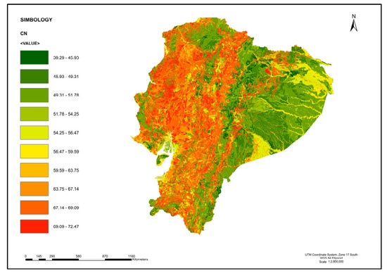
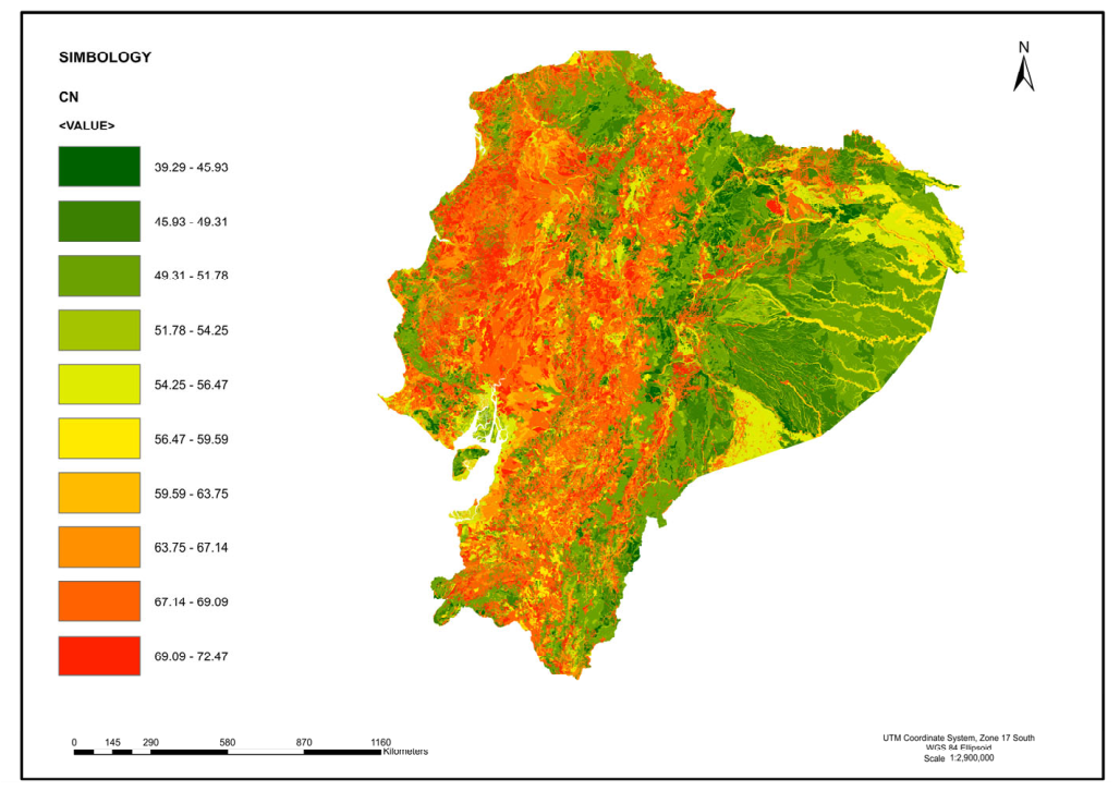
The Random Forest model generated a continuous 10 m resolution CN map for continental Ecuador (Figure 3) Predicted CN values ranged from approximately 30 in well-vegetated paramo areas underlain by freely draining soil (HSG A) to values approaching 90 in degraded agricultural zones with poorly draining clay soils on the coastal plain (HSG D). Regional CN statistics by physiographic region are shown in Table 5.

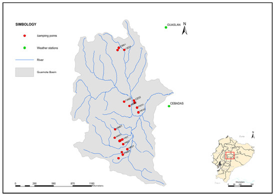
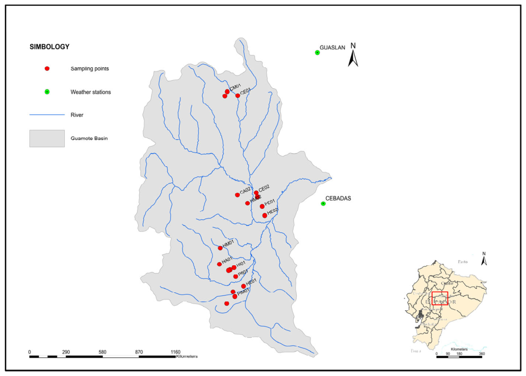
Figure 3. Guamote microwatershed showing the drainage network, field sampling locations used for hydraulic characterization and CN validation, and rain gauge stations used as precipitation inputs for the HEC-HMS simulations.

Table 5. Regional CN statistics from the Random Forest model.

Physiographic Region	Dominant Land Cover	CN Range (Field-Derived)	Mean CN (Expected)	HSG Dominant
Andean Highlands (Sierra)	Paramo/Shrub/cultivated	30–78	~55	A-B
Coastal lowlands	Cultivated/degrade/agricultural	69–99	~75	B-D
Amazon	Dense forest/Natural vegetation	30–55	~40	A-B

Note: Regional CN ranges derived from field-validated HSG assignments (Table 3) and SCS-USDA lookup tables applied to MAG geo-pedological layers.

The spatial distribution of CN showed expected physical gradients consistent with the SCS-USDA framework. In the Andean Highlands, CN exhibited spatial variability driven by sharp transitions between paramo, shrub vegetation, cultivated land, and forest plantations at small horizontal scales, a pattern consistent with the intra-class CN variability documented during field characterization in the Guamote watershed (Table 3). Coastal lowlands showed higher mean CN values, reflecting the combined effect of intense agricultural land use and fine-textured soil with restricted natural drainage. Amazon basins displayed intermediate to low CN values, consistent with dense broadleaf forest cover and high infiltration capacity across predominant HSG A and B soils. These regional gradients confirm that the model captured the dominant physical controls of runoff generation across Ecuador’s three major physiographic regions.

3.2. Model Performance Against the Nationally Distributed CN Map with Field-Anchored Hydrological Benchmarking

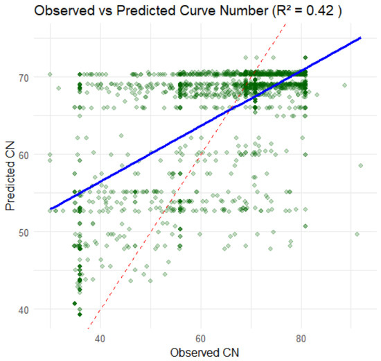
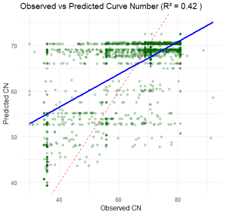
Performance evaluation on the 30% holdout validation subset (n = 6000 pixels) yielded RMSE = 10.4 CN units, R² = 0.42 and NSE = 0.41 (Figure 4). Because observed discharge records were unavailable, these metrics quantify the RF model’s ability to reproduce the spatial structure of the tabulated CN reference raster, not agreement with observed streamflow. Hydrological consistency was evaluated separately through the SDR/SRI framework described in Section 2.4. The RF model explained 42% of the spatial variance (R² = 0.42) of the hydrologically benchmarked tabulated CN raster—representing variance explained, not prediction error—and predictions remained within the physically plausible range defined by the SCS-USDA framework (CN 25–99), where 25 represents well-vegetated páramo on freely draining HSG A soils and 99 represents permanent water bodies; no predictions fell below 25 or above 99, confirming that the model did not extrapolate beyond the domain of the training reference. The mean prediction bias was below 2 CN units across highlands and Amazon validation points, indicating no systematic directional error in these regions. Larger positive biases (mean ∆CN up to + 12 CN units) were concentrated in coastal watersheds, where the model tended to overestimate CN relative to the tabulated reference, likely reflecting the unresolved fine-scale soil heterogeneity of alluvial coastal plains at the 1:25,000 mapping resolution.

Figure 4. Distributed 10 m Curve Number (CN) map for continental Ecuador derived from Random Forest modelling of official MAG geo-pedological layers. Coordinate reference system: UTM WGS84 Zone 17S. CN values represent the predicted direct runoff potential under average antecedent moisture conditions (AMC-II). Data sources and predictor variables are described in Table 1.

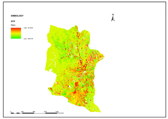
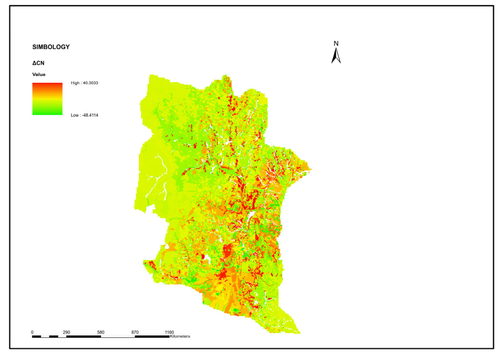
To further evaluate the spatial agreement between the RF prediction and the hydrologically benchmarked tabulated CN raster, a delta CN map was generated using the equation ΔCN = CN_RF − CN_Reference, where CN_RF is the Random Forest-predicted CN surface and CN_Reference is the hydrologically benchmarked CN reference raster used for model training (Figure 5). This map does not compare two independent nationwide CN datasets. Rather, CN_Reference is the field-anchored tabulated raster that served as the training target for the RF model; therefore, ΔCN quantifies the spatial deviation of the RF generalization relative to that benchmarked reference.

Figure 5. Spatial deviation map of the Random Forest Curve Number model (ΔCN = CN_RF − CN_Reference).

The resulting differences ranged from −48.4 to +40.3 CN units, with a near-zero mean difference (0.08 CN units) and a standard deviation of 12.4 CN units. These results indicate the absence of systematic overestimation or underestimation by the RF model at the national scale. Most differences remained within ±10 CN units across the mapped domain, reflecting strong agreement between the RF prediction and the benchmarked reference raster. Larger deviations were concentrated locally in transitional land cover mosaics, steep Andean terrain, and heterogeneous coastal alluvial systems, where non-linear interactions among terrain, soil drainage, and land use are more complex than those represented in the tabulated SCS-USDA framework.

It is important to note that the evaluation metrics reported here quantify the Random Forest model’s capacity to reproduce the spatial structure of the tabulated CN baseline through learned non-linear relationships among predictor variables, not its agreement with directly observed runoff measurements. This distinction is methodologically relevant; the RF model generalizes across spatial configurations not explicitly represented, and reference CN values partly reflect the model’s ability to interpolate across under-sampled spatial configurations rather than systematic error in runoff estimation.

This level of statistical performance is consistent with reported CN estimation studies incorporating field data. Shi et al. [11] reported R² values of 0.38–0.51 for CN prediction at slope scale in China, Walega et al. [12] obtained an RMSE of 8–13 CN units in forested watersheds of the southeastern United States, and Verma et al. [27] reported NSE values of 0.35–0.48 across a large multiwatershed dataset. The inherent empirical uncertainty of the CN method, well-documented by Hawkins [28] and Ponce and Hawkins [4], produces high scatter even under controlled field conditions, making statistical agreement in CN modelling rarely comparable to that achieved in physics-based model calibration. The relationship between the tabulated reference CN values and the Random Forest predictions for the holdout validation subset is presented in Figure 6.

Figure 6. Tabulated reference CN versus Random Forest predicted CN for the 30% holdout validation subset (n = 6000 pixels). The dashed line represents the 1:1 reference; the solid line represents the linear regression fit. Marginal distributions show the frequency of reference and predicted CN values across the validation sample.

3.3. Spatial Validation: Zonal CN Comparison Across Watershed Units

Zonal statistics computed per Level III Pfafstetter watershed polygon revealed that differences between Random Forest predictions and the tabulated reference CN raster (∆CN = CN_RF − CN_ref) were generally within ±5 CN units for watersheds in the Andean highlands and Amazon regions.

Larger absolute discrepancies (∆CN up to +12 CN units in some cases) were observed in coastal watersheds characterized by high subwatershed textural variability, particularly in sectors where alluvial deposits with contrasting drainage properties occur at scales finer than 1:25,000 geo-pedological mapping resolution. In these cases, the Random Forest model, trained on the dominant texture class per pixel, tended to overestimate CN relative to the tabulated reference, likely because the fine-scale mosaic of well-drained and poorly drained soils characteristic of coastal alluvial plains was not fully resolved by the input data.

The Guamote microwatershed, for which an independent HEC-HMS hydrological validation over 41 years is available, showed a mean ∆CN of less than 4 CN units between predicted and tabulated reference values. The result confirms that the distributed Random Forest model reproduces spatial CN patterns physically consistent with the independently validated rainfall-runoff response of the watershed, providing the strongest available hydrological benchmark for interpreting model performance at the national scale. The spatial convergence between machine learning predictions and the field-calibrated hydrological model constitutes the primary evidence supporting the applicability of the nationally distributed CN map with field-anchored hydrological benchmarking in a representative Andean watershed.

3.4. Predictor Variable Importance

Variable importance analysis based on mean decrease in node impurity (IncNodePurity) confirmed that land use (CUT II) and soil surface texture were the dominant predictors of CN spatial variability at the national scale, together accounting for 80.54% of total node impurity reduction. This result is physically consistent with the SCS-USDA framework, in which CN is determined primarily by the combination of land cover category and Hydrologic Soil Group, the latter of which is derived directly from soil texture and drainage class. The relative contribution of each predictor variable to the Random Forest model is summarized in Table 6.

Table 6. Relative variable importance of predictor variables in the Random Forest CN model.

Predictor Variable	Relative Importance (%)	Physical Role in CN Framework
Land use (CUT II)	66.01	Determines vegetation cover category in CN tables
Surface texture	14.53	Determines Hydrologic Soil Group (HSG)
Natural drainage	12.02	Refines hydrological soil behavior
Topographic slope	7.44	Adjustment factor in steep Andean terrain

Natural drainage ranked third in importance, contributing 12.02% of node impurity reduction. Its role was particularly pronounced in volcanic soil environments and poorly drained sectors of the coastal plain, where texture class alone does not fully resolve HSG assignment and drainage class provides critical discriminating information. Topographic slope ranked fourth (7.44% of node impurity reduction), reflecting its secondary role as an adjustment factor in the CN method. Nevertheless, slope contributed meaningful spatial refinement in high-relief Andean areas where terrain gradient directly conditions overland flow generation and concentration time, consistent with reported evidence on CN adjustment for steep terrain [11,29].

4. Discussion

4.1. Contribution to Distributed CN Estimation in Data-Scarce Andean Regions

This study presents, to our knowledge, the first national-scale distributed CN map for Ecuador grounded in a hydrologically benchmarked training reference. Previous CN applications in the country have been restricted to individual microwatersheds or administrative units using aggregated tabulated values, without spatial continuity or independent hydrological validation [10,24]. At the broader Latin America scale, national-scale distributed CN mapping remains largely absent from the peer-reviewed literature; most published applications in the region employ watershed-average CN values derived directly from SCS-USDA tables without spatial disaggregation or field-based calibration [23,27]. By integrating the MAG 1:25,000 p-pedological datasets with Random Forest regression and a field-anchored training reference, the proposed workflow addresses a critical methodological gap in Andean hydrology: the availability of spatially explicit, physically consistent CN estimates for distributed modeling in territories where continuous discharge records are absent.

Similar national-scale mapping efforts have been reported for China [30], the United States [31], and selected European catchments [16]. What distinguishes the present approach is not the resolution or the algorithm, Random Forest has been applied to CN estimation before, but the nature of the training reference. In those studies, model performance is measured against SCS-USDA lookup values, which means that the model can score well statistically while doing little more than reproducing the tabulated assumptions embedded in its own training data. Here, the CN reference raster was anchored to independently observed discharge before being used for training. That step, modest as it may appear, changes what the performance metrics mean: they no longer describe how well the model reproduces a table, but how well it captures spatial CN patterns that are physically consistent with measured runoff behavior.

4.2. Interpretation of Model Performance Metrics

The R² of 0.42 and NSE of 0.41 obtained on the holdout validation subset reflect inherent empirical uncertainty of the CN method, a well-documented characteristic of the SCS-USDA framework. Hawkins [32] demonstrated that asymptotic CN determination from observed rainfall-runoff data routinely produces high scatter regardless of sample size, and Ponce and Hawkins [4] noted that statistical agreement in CN modeling is rarely comparable to that achieved in physics-based model calibration. In this context, the performance metrics reported here are consistent with reported CN estimation studies incorporating field data; Shi et al. [11] reported R² of 0.38–0.51 for CN prediction at slope scale in China, Walega et al. [12] obtained RMSE values of 8–13 CN units in forested watersheds of the southeastern United States [27] reported NSE values of 0.35–0.48 across a large multiwatershed dataset. A comparison between the performance of the present Random Forest model and previously published field-based CN estimation studies is summarized in Table 7.

Table 7. Comparison of Random Forest CN model performance with published field-based CN estimation studies.

Study	Region	Method	RMSE	R2	NSE
This study	Ecuador (national)	Random Forest	10.4	0.42	0.41
Shi et al. [11]	China (slope scale)	Statistical	-	0.38–0.51	-
Walega et al. [12]	SE United States	SCS-CN modified	8–13	-	-
Verma et al. [27]	USA (multiwatershed)	Regression	-	-	0.35–0.48

Watershed-scale CN averages, rather than pixel-level point estimates, are the primary input parameter to distributed hydrological models such as HEC-HMS and SWAT [20,31,32,33]. The spatial validation through zonal comparison, which confirmed mean absolute ∆CN below 5 units across Andean highland and Amazon watersheds, therefore provides more operationally relevant evidence of model utility than pixel-level RMSE alone. A model that reproduces correct watershed-scale CN averages will produce consistent inputs to these tools even if pixel-level scatter is moderate, which is precisely what the zonal validation demonstrates for the Guamote watershed and the broader highland and Amazon regions.

4.3. Role and Scope of the Field-Based Hydrological Validation

The HEC-HMS model for the Guamote microwatershed, driven by 41 years of daily precipitation data (1981–2021) and parameterized with the field-anchored tabulated CN values, produced a mean annual discharge of 0.1568 m³ s⁻¹, a result consistent with the observed hydrological regime of Andean m³-agricultural systems in central Sierra [24]. This hydrologically benchmarked discharge estimate constitutes a physical anchor for interpreting the national machine learning predictions. The fact that the Random Forest reproduces spatial CN patterns with a mean ∆CN below 4 units in the Guamote watershed, where the CN reference has been independently confirmed through long-term hydrological modeling, provides direct evidence that the distributed model captures the dominant runoff-generating mechanisms of the Andean landscape. Preliminary sensitivity analysis within the HEC-HMS framework confirmed that applying spatially uniform watershed-average CN values derived directly from SCS-USDA tables without spatial disaggregation produced lower discharge consistency relative to SENAGUA-authorized water demand compared to the spatially distributed RF-based CN raster, supporting the added value of the distributed approach over conventional aggregated tabulation.

Most CN studies that employ machine learning assess model performance against the same tabulated CN values used to build the training dataset. The result is a closed loop: good statistical scores are almost guaranteed because the model is essentially being asked whether it has learned the lookup table. The approach taken here deliberately opens that loop. By training the national Random Forest model on a CN reference raster that has already been confirmed against 41 years of observed discharge in Guamote, the evaluation acquires an external physical anchor. When the model then achieves ∆CN <4 units in that watershed, the agreement is not between two products of the same table; it is between a machine learning prediction and a hydrologically calibrated field measurement. That difference is what justifies describing the result as physically meaningful rather than merely statistically acceptable.

4.4. Limitations and Directions for Future Research

The primary limitation of this study is the geographic scope of the field-based hydrological validation, which is anchored in a single microwatershed (Guamote) located in the central Andes. While spatial validation through zonal CN comparison extends model evaluation to the national scale, the hydrological benchmark remains localized to one physiographic context. The extent to which the field-derived HSG assignments and CN values from Guamote are representative of soil hydraulic behavior in coastal alluvial plains and Amazon lowland forests cannot be fully assessed from the available data. Future research should integrate additional field-characterized CN datasets and independent discharge records from coastal and Amazon basins to broaden the hydrological validation scope.

A second limitation concerns the static nature of the predictor variables. Dynamic controls on CN, particularly antecedent soil moisture conditions (AMC classes I through III) and seasonal land cover change, were not incorporated into the moisture conditions (AMC-II). Incorporating satellite-derived soil moisture or seasonal vegetation as time-varying predictors could enable dynamic CN estimation and improve model performance under extreme wet or dry antecedent conditions. Future work should explore temporal CN variability associated with land cover change trajectories, building on the paired-watershed monitoring framework developed for the Jatunchimbana and Gualcanga basins [29,34].

A third limitation relates to the spatial resolution mismatch between the 1:25,000 geo-pedological input data and the 10 m pixel output. The effective spatial resolution of the CN predictors is constrained by the coarsest input layer rather than by the DEM pixel size. Subwatershed soil heterogeneity at scale finer than the mapping unit (1–5 ha at 1:25,000) is not resolved by the model, which likely explains the larger ∆CN values observed in coastal watershed with high textural variability. Future studies should evaluate the potential of integrating higher-resolution soil data sources to improve spatial fidelity in heterogeneous pedological environments.

4.5. Practical Relevance for Water Resources Planning and SDG Alignment

The 10 m national CN map produced by this study provides a spatially explicit, field-grounded parameterization layer directly applicable to distributed hydrological modeling tools such as HEC-HMS and SWAT. In the predominantly data-scarce context of the Ecuadorian Andes and Amazon, the availability of a physically consistent, high-resolution CN map represents a substantive improvement over the current practice of assigning single tabulated CN values per administrative or watershed unit. Practical applications include water irrigation demand estimation under different land use scenarios, prioritization of watershed conservation investments based on spatially explicit runoff potential, and parameterization of climate adaptation models that require spatially distributed infiltration inputs.

The reproducible geospatial workflow is designed for direct replication in other data-scarce Andean and tropical territories where MAG-equivalent geo-pedological datasets exist. By generating spatially explicit runoff potential estimates that support watershed planning, flood risk screening, conservation prioritization, and climate adaptation, this work contributes to decision-support frameworks aligned with SDG 6 (clean water and sanitation), SDG 11 (sustainable cities), SDG 13 (climate action) and SDG 15 (life on land).

5. Conclusions

This study produced a distributed Curve Number estimation at 10 m spatial resolution for continental Ecuador by combining official MAG geo-pedological layers at 1:25,000 scale with a Random Forest regression model. The principal methodological decision, training the model on a CN reference raster anchored to field-measured hydraulic parameters and 41 years of HEC-HMS discharge modeling in the Guamote microwatershed, distinguishes this work from CN estimation studies that evaluate machine learning models against the same lookup tables used to construct their training data. To our knowledge, no equivalent field-anchored distributed CN mapping workflow at national scale has been previously reported for an Andean country.

Model performance (RMSE = 10.4 CN units; R² = 0.42; NSE = 0.41) falls within the range documented in published field-based CN studies and is best understood considering the SCS-USDA method’s own empirical scatter rather than as a limitation of the Random Forest approach. More telling than the pixel-level metrics is the spatial validation: mean absolute ∆CN remained below 5 CN units across Andean highland and Amazon watersheds and below 4 units in Guamote specifically, where an independent hydrological model provides the benchmark. At the watershed scale at which CN values enter tools like HEC-HMS and SWAT, the map provides a consistent and physically interpretable input.

Land use and land surface texture dominated variable importance, as expected from the structure of the SCS-USDA framework. Natural drainage contributed meaningfully where texture alone could not resolve hydrological group assignment, particularly in volcanic soils and poorly drained coastal sectors, while topographic slope provided refinement in high-relief Andean terrain. Together, the four MAG predictor layers, despite their 1:25,000 nominal scale, proved sufficient to capture the primary spatial controls of runoff generation to a national extent.

The workflow is reproducible, built on open-source tools and publicly available official datasets, and designed to transfer. Other countries in Latin America and the tropics face the same combination of physiographic complexity, data scarcity, and growing demand for spatially explicit hydrological inputs. The geo-pedological datasets now being produced across the region create the conditions to replicate this approach elsewhere.

6. Patents

The methodology and software used in this study are associated with registered software titled “Calculadora del Número de Curva (CN)”, officially registered at the National Service for Intellectual Rights (SENADI), Ecuador.

References

- Mockus, V. Soil Conservation Service (SCS) National Engineering Handbook; Scientific Research Publishing: Glendale, CA, USA, 1964. [Google Scholar]
- Van Thinh, L.; Yadav, I.C.; Boulange, J.; Thuyet, D.Q.; Watanabe, H. Modeling of Runoff Water and Runoff Pesticide Concentrations in Upland Bare Soil Using Improved SPEC Model. J. Pestic. Sci. 2019, 44, 148–155. [Google Scholar] [CrossRef] [Scilit] [PubMed]
- Hawkins, R.H. Asymptotic Determination of Runoff Curve Numbers from Data. J. Irrig. Drain. Eng. 1993, 119, 334–345. [Google Scholar] [CrossRef] [Scilit]
- Ponce, V.M.; Hawkins, R.H. Runoff Curve Number: Has It Reached Maturity? J. Hydrol. Eng. 1996, 1, 11–19. [Google Scholar] [CrossRef] [Scilit]
- Mishra, S.K.; Singh, V.P. Soil Conservation Service Curve Number (SCS-CN) Methodology, 1st ed.; Springer Science & Business Media: Berlin/Heidelberg, Germany, 2003; Volume 42, ISBN 978-94-017-0147-1. [Google Scholar]
- Beven, K.J. Rainfall-Runoff Modelling: The Primer; John Wiley & Sons: Hoboken, NJ, USA, 2012; ISBN 047071459X. [Google Scholar]
- do Valle Junior, L.C.G.; Rodrigues, D.B.B.; de Oliveira, P.T.S. Initial Abstraction Ratio and Curve Number Estimation Using Rainfall and Runoff Data from a Tropical Watershed. Rbrh 2019, 24, e5. [Google Scholar]
- Lian, H.; Yen, H.; Huang, J.-C.; Feng, Q.; Qin, L.; Bashir, M.A.; Wu, S.; Zhu, A.-X.; Luo, J.; Di, H.; et al. CN-China: Revised Runoff Curve Number by Using Rainfall-Runoff Events Data in China. Water Res. 2020, 177, 115767. [Google Scholar] [CrossRef] [Scilit] [PubMed]
- Woodward, D.E.; Hawkins, R.H.; Jiang, R.; Hjelmfelt Allen, T.J.; Van Mullem, J.A.; Quan, Q.D. Runoff Curve Number Method: Examination of the Initial Abstraction Ratio. In Proceedings of the World Water & Environmental Resources Congress; American Society of Civil Engineers (ASCE): Reston, VA, USA, 2003; pp. 1–10. [Google Scholar]
- Atre, A.A.; Sthool, V.A.; Barhate, S.R. A Critical Look into Curve Number Method for Direct Runoff Estimation. J. Agric. Res. Technol. 2016, 41, 343. [Google Scholar]
- Shi, W.; Wang, M.; Bao, J.; Yu, J.; Chen, T.; Song, W.; Chen, H. An Improved Curve Number for Runoff Prediction under Different Vegetation Pattern at Slope Scale in China. Catena 2025, 249, 108641. [Google Scholar] [CrossRef] [Scilit]
- Walega, A.; Amatya, D.M.; Caldwell, P.; Marion, D.; Panda, S. Assessment of Storm Direct Runoff and Peak Flow Rates Using Improved SCS-CN Models for Selected Forested Watersheds in the Southeastern United States. J. Hydrol. Reg. Stud. 2020, 27, 100645. [Google Scholar] [CrossRef] [Scilit]
- Ibrahim, A.; Wageeh, A.; Hamouda, M.A.; Ahmed, A.; Gad, A. Impact of LULC Classification Methods on Runoff Simulation in an Arid Mountainous Watershed Using Remote Sensing and Machine Learning. Earth 2026, 7, 26. [Google Scholar] [CrossRef] [Scilit]
- Özdemir, A.; Erdoğan, H.; Özkaynak, H.; Öztürk, B.; Coşkun, S.B. A Machine Learning Framework for Estimating Fragility Curves of Low-to Mid-Rise RC Buildings. Buildings 2026, 16, 2127. [Google Scholar] [CrossRef] [Scilit]
- Costache, R.; Bao Pham, Q.; Corodescu-Roșca, E.; Cîmpianu, C.; Hong, H.; Thi Thuy Linh, N.; Ming Fai, C.; Najah Ahmed, A.; Vojtek, M.; Muhammed Pandhiani, S. Using GIS, Remote Sensing, and Machine Learning to Highlight the Correlation between the Land-Use/Land-Cover Changes and Flash-Flood Potential. Remote Sens. 2020, 12, 1422. [Google Scholar] [CrossRef] [Scilit]
- Williams, J.R.; Kannan, N.; Wang, X.; Santhi, C.; Arnold, J.G. Evolution of the SCS Runoff Curve Number Method and Its Application to Continuous Runoff Simulation. J. Hydrol. Eng. 2012, 17, 1221–1229. [Google Scholar] [CrossRef]
- Mosavi, A.; Ozturk, P.; Chau, K. Flood Prediction Using Machine Learning Models: Literature Review. Water 2018, 10, 1536. [Google Scholar] [CrossRef] [Scilit]
- Belgiu, M.; Drăguţ, L. Random Forest in Remote Sensing: A Review of Applications and Future Directions. ISPRS J. Photogramm. Remote Sens. 2016, 114, 24–31. [Google Scholar] [CrossRef] [Scilit]
- Breiman, L. Random Forests. Mach. Learn. 2001, 45, 5–32. [Google Scholar] [CrossRef] [Scilit]
- Verma, S.; Singh, P.K.; Mishra, S.K.; Jain, S.K.; Berndtsson, R.; Singh, A.; Verma, R.K. Simplified SMA-Inspired 1-Parameter SCS-CN Model for Runoff Estimation. Arab. J. Geosci. 2018, 11, 420. [Google Scholar] [CrossRef] [Scilit]
- Maldonado Chávez, C.A.; Larrea Berrones, A. Determinación de La Oferta Hídrica de La Microcuenca Guamote y Quebrada Compuene Gorge, En La Provincia de Chimborazo, Riobamba, Universidad Nacional de Chimborazo, 2023. Available online: http://dspace.unach.edu.ec/handle/51000/10251 (accessed on 15 June 2026).
- Rahman, M.; Islam, M.M.; Kim, H.-J.; Sadiq, S.; Alam, M.; Siddiqua, T.; Mamun, A.; Gazi, M.A.H.; Raju, M.R.; Chen, N. Assessing the Influence of Land Cover and Climate Change Impacts on Runoff Patterns Using CA-ANN Model and CMIP6 Data. ISPRS Int. J. Geo-Inf. 2023, 12, 401. [Google Scholar] [CrossRef] [Scilit]
- Sreejith, K.S.; Kumar, G.P.; Dwarakish, G.S. A Critical Review of the Soil Conservation Services–Curve Number Method in Hydrological Modelling. Wetlands 2024, 44, 117. [Google Scholar] [CrossRef] [Scilit]
- Ministerio de Agricultura y Ganadería del Ecuador Mapa Geopedológico Del Ecuador Continental, Versión Editada 2019, Escala 1:25.000, Año 2009–2015. Available online: http://geoportal.agricultura.gob.ec/index.php/visor-geo (accessed on 15 June 2026).
- JAXA ALOS World 3D–30 m (AW3D30) Digital Surface Model. Available online: https://search.asf.alaska.edu/#/?zoom=3.000¢er=-97.494,39.673&dataset=ALOS-2 (accessed on 15 June 2026).
- Chidichimo, F.; Mendoza, B.T.; De Biase, M.; Catelan, P.; Straface, S.; Di Gregorio, S. Hydrogeological Modeling of the Groundwater Recharge Feeding the Chambo Aquifer, Ecuador. AIP Conf. Proc. 2018, 2022, 020003. [Google Scholar] [CrossRef] [Scilit]
- Verma, S.; Verma, R.K.; Mishra, S.K.; Singh, A.; Jayaraj, G.K. A Revisit of NRCS-CN Inspired Models Coupled with RS and GIS for Runoff Estimation. Hydrol. Sci. J. 2017, 62, 1891–1930. [Google Scholar] [CrossRef] [Scilit]
- Feldman, A.D. Hydrologic Modeling System HEC-HMS: Technical Reference Manual; US Army Corps of Engineers, Hydrologic Engineering Center: Glendale, CA, USA, 2000. [Google Scholar]
- Bonta, J.V.; Cleland, B. Incorporating Natural Variability, Uncertainty, and Risk into Water Quality Evaluations Using Duration Curves. JAWRA J. Am. Water Resour. Assoc. 2003, 39, 1481–1496. [Google Scholar] [CrossRef] [Scilit]
- Shi, W.; Wang, N. An Improved SCS-CN Method Incorporating Slope, Soil Moisture, and Storm Duration Factors for Runoff Prediction. Soil Conserv. Serv. Curve Number (SCS-CN) Method Curr. Appl. Remain. Chall. Future Perspect. 2020, 12, 1335. [Google Scholar] [CrossRef] [Scilit]
- Xia, C.; Zhang, L.; Zhu, Z.; Xia, H.; Tian, H. A Multi-Temporal Scale Framework for Comprehensive Quantification and Attribution of Anthropogenic Impacts on Runoff. Sci. Rep. 2025, 16, 1965. [Google Scholar] [CrossRef] [Scilit] [PubMed]
- Boulesteix, A.; Janitza, S.; Kruppa, J.; König, I.R. Overview of Random Forest Methodology and Practical Guidance with Emphasis on Computational Biology and Bioinformatics. Wiley Interdiscip. Rev. Data Min. Knowl. Discov. 2012, 2, 493–507. [Google Scholar] [CrossRef] [Scilit]
- Yang, J.; Li, C.; Li, L.; Ding, J.; Zhang, R.; Han, T.; Liu, Y. Automatic Detection of Regional Snow Avalanches with Scattering and Interference of C-Band SAR Data. Remote Sens. 2020, 12, 2781. [Google Scholar] [CrossRef] [Scilit]
- Tripathi, A.; Attri, L.; Tiwari, R.K. Spaceborne C-Band SAR Remote Sensing–Based Flood Mapping and Runoff Estimation for 2019 Flood Scenario in Rupnagar, Punjab, India. Environ. Monit. Assess. 2021, 193, 110. [Google Scholar] [CrossRef] [Scilit] [PubMed]
Disclaimer/Publisher’s Note: The statements, opinions and data contained in all publications are solely those of the individual author(s) and contributor(s) and not of MDPI and/or the editor(s). MDPI and/or the editor(s) disclaim responsibility for any injury to people or property resulting from any ideas, methods, instructions or products referred to in the content. |
© 2026 by the authors. Licensee MDPI, Basel, Switzerland. This article is an open access article distributed under the terms and conditions of the Creative Commons Attribution (CC BY) license.